self-optimizing control structures for active constraint regions...

Self-Optimizing Control Structures for Active Constraint Regions of a Sequence of Distillation Columns

Roald Bræck Leer

Chemical Engineering and Biotechnology

Supervisor: Sigurd Skogestad, IKPCo-supervisor: Johannes Jäschke, IKP

Department of Chemical Engineering

Submission date: July 2012

Norwegian University of Science and Technology

Abstract

Investigating and mapping active constraint regions for processes, and subsequentlyfinding control structures for each region, is vital for their optimal operation. Inthis work, active constraint regions of three different case studies for the distillationprocess have been investigated:

• A single distillation column with constant product prices.

• A single distillation column with purity dependent prices.

• Two distillation columns in sequence with constant prices.

The active constraint regions for each case study have been identified and mappedwith respect to the disturbances; energy price and feed flow rate. Selected stagetemperatures and combinations of stage temperatures have been proposed as self– optimizing variables for the unconstrained degrees of freedom of each region.These were found by the use of the Minimum Singular Value Rule and the ExactLocal Method. The methods requires the optimal sensitivities of measurementswith respect to disturbances, which was obtained by using the software packageIpopt/sIpopt.

To demonstrate applicability, a selection of the control structures for the differentregions of each case study have been implemented and compared on the dynamicnonlinear models using Simulink.

It has been shown that the first case study, a single distillation column with constantproduct prices, has 3 active constraint regions while the next, a single distillationcolumn with purity dependent prices, has 5 active constraint regions. The lastcase study, two distillation columns in sequence with constant prices, has 8 activeconstraint regions.

i

Sammendrag

Undersøking og kartlegging av aktive begrensningsomrader for prosesser, for derettera finne reguleringsstrukturer for hver region, er avgjørende for deres optimale drift.Dette arbeidet tar for seg aktive begrensningsomrader for tre forskjelliger studierav destillasjon:

• En enkel destillasjonskolonne med faste priser.

• En enkel destillasjonskolonne hvor produktprisen er proposjonal renheten avproduktet.

• To destillasjonskolonner i serie med faste priser.

De aktive begrensningsomradene for hver studie har blitt identifisert og kartlagtmed hensyn pa forstyrrelsene energipris og fødehastighet. I hvert omrade har utval-gte trinntemperaturer og kombinasjoner av trinntemperaturer blitt foreslatt somselv – optimaliserende variabler for de ubrukte frihetsgradene. Disse ble funnet vedbruk av Minimum Singular Value Rule og Exact Local Method. For a bruke de tometodene trengs de optimale sensitivitene til malingene. Dataverktøyet sIpopt blebrukt til dette.

Noen av de foreslatte reguleringsstrukturene for de ulike omradene i hver studiehar blitt implementert og sammenlignet pa de dynamiske ikke – lineære modellenei Simulink.

Det har blitt vist at første studie, en enkelt destillasjonkolonne med faste pro-duktpriser, har 3 aktive begrensningsomrader. Neste studie, en enkelt destil-lasjonkolonne hvor produktprisen er proposjonal renheten av produktet, har 5 ak-tive begrensningsomrader. Den siste studien, to destillasjonskolonner i serie medfaste priser, har 8 aktive begrensningsomrader.

iii

Preface

This thesis was written as the final part of my M.sc degree in Chemical engineeringat the Norwegian University of Science and Technology.

First, I would like to express my profound gratitude to my supervisors, Post-doc Johannes Jasckhe, and Professor Sigurd Skogestad for their invaluable helpthroughout my work with this thesis.

Thank you both!

Second, I would also like to thank my friends at the Process-systems engineer-ing group for the good companionship. Especially the weekly fotball sessions havebeen memorable.

Declaration of Compliance

I hereby declare that this is an independent work in compliance with the examregulations of the Norwegian University of Science and Technology.

Trondheim, July 5, 2012

Roald Bræck Leer

v

Contents

1 Introduction 1

1.1 Problem Description . . . . . . . . . . . . . . . . . . . . . . . . . . . 2

2 Background 3

2.1 Distillation . . . . . . . . . . . . . . . . . . . . . . . . . . . . . . . . 3

2.2 Optimization . . . . . . . . . . . . . . . . . . . . . . . . . . . . . . . 7

2.3 Numerical Tools . . . . . . . . . . . . . . . . . . . . . . . . . . . . . 8

2.3.1 Matlab/Simulink . . . . . . . . . . . . . . . . . . . . . . . . . 8

2.3.2 Ipopt . . . . . . . . . . . . . . . . . . . . . . . . . . . . . . . 8

2.3.3 sIpopt . . . . . . . . . . . . . . . . . . . . . . . . . . . . . . . 8

2.3.4 AMPL . . . . . . . . . . . . . . . . . . . . . . . . . . . . . . . 8

2.4 Self – optimizing Control . . . . . . . . . . . . . . . . . . . . . . . . 9

2.4.1 Minimum Singular Value Rule . . . . . . . . . . . . . . . . . 11

2.4.2 Exact Local Method . . . . . . . . . . . . . . . . . . . . . . . 13

3 Cases 15

3.1 Model . . . . . . . . . . . . . . . . . . . . . . . . . . . . . . . . . . . 16

3.2 Case Study 1a . . . . . . . . . . . . . . . . . . . . . . . . . . . . . . 16

3.2.1 Degrees of Freedom . . . . . . . . . . . . . . . . . . . . . . . 17

3.2.2 Disturbances . . . . . . . . . . . . . . . . . . . . . . . . . . . 17

3.2.3 Optimization Problem . . . . . . . . . . . . . . . . . . . . . . 18

3.2.4 Constraints . . . . . . . . . . . . . . . . . . . . . . . . . . . . 18

3.3 Case Study 1b . . . . . . . . . . . . . . . . . . . . . . . . . . . . . . 19


3.3.2 Disturbances . . . . . . . . . . . . . . . . . . . . . . . . . . . 19


3.3.4 Constraints . . . . . . . . . . . . . . . . . . . . . . . . . . . . 19

3.4 Case study 2 . . . . . . . . . . . . . . . . . . . . . . . . . . . . . . . 20


3.4.2 Disturbances . . . . . . . . . . . . . . . . . . . . . . . . . . . 21


3.4.4 Constraints . . . . . . . . . . . . . . . . . . . . . . . . . . . . 21

vii

viii Contents

4 Results 234.1 Active Constraint Regions . . . . . . . . . . . . . . . . . . . . . . . . 23

4.1.1 Case Study 1a . . . . . . . . . . . . . . . . . . . . . . . . . . 234.1.2 Case Study 1b . . . . . . . . . . . . . . . . . . . . . . . . . . 244.1.3 Case Study 2 . . . . . . . . . . . . . . . . . . . . . . . . . . . 25

4.2 Self – optimizing variables . . . . . . . . . . . . . . . . . . . . . . . . 284.2.1 Minimum Singular Value Rule . . . . . . . . . . . . . . . . . 284.2.2 Case Study 1a . . . . . . . . . . . . . . . . . . . . . . . . . . 284.2.3 Case Study 1b . . . . . . . . . . . . . . . . . . . . . . . . . . 294.2.4 Case Study 2 . . . . . . . . . . . . . . . . . . . . . . . . . . . 294.2.5 Exact Local Method . . . . . . . . . . . . . . . . . . . . . . . 34

4.3 Simulations . . . . . . . . . . . . . . . . . . . . . . . . . . . . . . . . 354.3.1 Case Study 1a . . . . . . . . . . . . . . . . . . . . . . . . . . 354.3.2 Case Study 1b . . . . . . . . . . . . . . . . . . . . . . . . . . 364.3.3 Case Study 2 . . . . . . . . . . . . . . . . . . . . . . . . . . . 37

5 Discussion 395.1 Maps of the Active Constraint Regions . . . . . . . . . . . . . . . . . 39

5.1.1 Comparison With Previous Work . . . . . . . . . . . . . . . . 405.2 Minimum Singular Value Rule . . . . . . . . . . . . . . . . . . . . . . 425.3 Simulations . . . . . . . . . . . . . . . . . . . . . . . . . . . . . . . . 435.4 Ipopt/sIpopt . . . . . . . . . . . . . . . . . . . . . . . . . . . . . . . 43

6 Conclusion 45

7 Further Work 47

A Combinations of temperatures as self – optimizing variables 51

B Pairing 57B.1 Case study 1a . . . . . . . . . . . . . . . . . . . . . . . . . . . . . . . 57B.2 Case study 1b . . . . . . . . . . . . . . . . . . . . . . . . . . . . . . . 58B.3 Case study 2 . . . . . . . . . . . . . . . . . . . . . . . . . . . . . . . 59

C Temperature profiles 63C.1 Case 1a . . . . . . . . . . . . . . . . . . . . . . . . . . . . . . . . . . 63C.2 Case 1b . . . . . . . . . . . . . . . . . . . . . . . . . . . . . . . . . . 64C.3 Case 2 . . . . . . . . . . . . . . . . . . . . . . . . . . . . . . . . . . . 65

D AMPL code 69

Chapter 1

Introduction

Today, separation of chemical components plays an important part of modern life.Whether it is industrial large scale separation or small scale separation performedin a lab. Separation is defined as as:

“A process of any scale by which the components of a mixture are sepa-rated from each other without substantial chemical modification”(Cooke& Poole 2000)

The range and scope of the different techniques are numerous to accommodate forall the different separation processes. Distillation is a commonly used separationprocess in the chemical industry. It is used substantially in the oil and gas sector.E.g. when refined, crude oil is separated by distillation into fractions of naphtha,diesel, gas, jet fuel, etc. With the new boom in the oil industry and an ever presentneed for fossil fuels, the focus on research and innovation in this area is crucial.

Over the years, distillation has been thoroughly researched and documented. Con-trol of distillation columns is also well investigated in numerous books and articles.However, there has been surprisingly few investigations into optimal operation andactive constraints, as pointed out by Jacobsen in his thesis (Jacobsen 2011).

To ensure optimal operation one needs to know how the active constraints changewith respect to disturbances. A control structure for one active constraint regionmay not be feasible for another region where different constraints are active. Locat-ing and mapping these regions provides useful information when choosing controlstructures.

Selection of good controlled variables and implementing these in a control structureplays an important part of optimal operation. The term “good controlled variables”reflects the basis for the idea of self – optimizing control (Skogestad 2000). Findingand controlling some key variables to a constant value so that the process runsclose to an optimum.

1

2 Introduction

These variables may be found by applying different methods, like the MinimumSingular Value Rule(Skogestad & Postletwaite 1996) and the Exact Local Method(Halvorsen, Skogestad, Morud & Alstad 2003) to a set of measurements.

This work is twofold. Locating and mapping the active constraint regions for thedifferent case studies, and proposing self – optimizing control structures for eachregion. Also, the software package Ipopt/sIpopt (Wachter & Biegler 2006) is usedin this work to test it on a self – optimizing control study.

1.1 Problem Description

This assignment continues on Magnus Jacobsen’s work of identifying active con-straint regions for optimal operation of distillation columns.

In his thesis Jacobsen examines the active constraint regions for three cases:

1. A single distillation column with constant product prices.

2. A single distillation column with purity dependent product prices.

3. Two distillation columns in sequence with constant prices.

Although identifying these regions, Jacobsen did not pursue finding the self – op-timizing variables for the unconstrained degrees of freedom. The purpose of thiswork is to find self – optimizing control structures for each of the active constraintregions previously found by Jacobsen. The idea is that by keeping certain variablesor combinations of variables constant, the distillation column will operate close tothe optimum without having to re-optimize for disturbances.

Mapping the active constraint regions for each of the cases will be redone to al-low for comparison of previous work. A steady – state distillation model will bewritten in the in the mathematical programming language AMPL (Fourer, Gay &Kerninghan 2003) and optimized using the open software Ipopt/sIpopt (Wachter& Biegler 2006). The model is based on the distillation Column A (Morari &Skogestad 1988).

In each of the active constraint regions the model will be linearized to find candi-dates for the self – optimizing controlled variables. The Minimum Singular ValueRule and the Exact Local Method will be used to find these. Selected self – optimiz-ing control structures will then be compared and tested on the dynamic nonlinearmodels using Matlab/Simulink.

Chapter 2

Background

In this chapter relevant theory for the thesis will be introduced. The process ofdistillation is presented and pertinent equations derived. Relevant optimizationtheory is gone through along with brief introductions of the tools used. The princi-ple behind self – optimizing control is explained as well as the methods for findingself – optimizing variables.

2.1 Distillation

Distillation is one of the most important separation technologies in the industry.It may be described as a countercurrent multistage flash. If you increase the num-ber of equilibrium stages almost any degree of separation, with a fixed energyconsumption, is possible (Halvorsen & Skogestad 2000). This makes distillationparticularly good for high purity separations. A simple schematic of a distillationstage is shown in Figure 2.1. Liquid is flowing downwards through the column,entering the stage from the top. It is mixed with the vapor flowing upwards andequilibrium is reached. This is distillation stage concept. At each theoretical stageone assumes that vapor – liquid equilibrium(VLE) is reached. This may not be truefor all columns, i.e. packed columns, but it has been established that the conceptfits well with experimental data from real columns (Halvorsen & Skogestad 2000).

For a two – component system, with Nc non reacting components, the state isdetermined by Nc degrees of freedom. The degrees of freedom, f , is given fromGibb’s phase rule:

f = Nc + 2− ph (2.1)

Here ph is the number of phases. Setting the pressure, P , and the liquid mole frac-tions, x, as degrees of freedom, the temperature, T , and the vapor mole fractions,y, are determined. The VLE then is written:

3

4 Background

Liquid entering the stage

Vapour phase

Liquid phase

Saturated liquid leaving the stage Vapour entering the stage

Perfect mixing in every stage

Saturated vapour leaving the stage

T p y

x

Figure 2.1: Equilibrium – stage concept.

[y1, y2 · · · , yNc−1] = f(P, x1, x2 · · · , xNc−1)

[y, T ] = f(P, x)(2.2)

The mole fractions in the liquid phase∑n

i=1 xi = 1 and in the vapor phase∑ni=1 yi = 1, where n is the number of stages. The familiar Raoult’s law states

that for ideal mixtures the partial pressure of a component in the vapor phase isproportional to the partial pressure of the pure component pi = xip

◦i (T ). Dalton’s

law for ideal gases states that the partial pressure of a component is proportionalto the mole fraction pi = yiP . Combining these two equations, and adding thatthe total pressure of the system is a combination of the partial pressures, one canderive the following relationship:

yi = xip◦iP

=xip◦i (T )∑

i xip◦i (T )

(2.3)

For a component i, the K – value is defined as follows:

Ki =yixi

(2.4)

2.1. Distillation 5

From the K – values the relative volatility is derived, which is a measure of com-paring the vapor pressures of the components in a liquid mixture. It is desirable tohave a large relative volatility when separating two components due to the implica-tion that there is a large difference between the boiling points of the components,making the separation easier. Applying Raoult’s law for ideal mixtures, the relativevolatility becomes:

αij =(yi/xi)

(yj/xj)=Ki

Kj=p◦i (T )

p◦j (T )(2.5)

The partial pressure is dependent on the temperature and thus the K – values aredependent on temperature. Combining Equations (2.3) and (2.5) gives the VLE –relationship. For a binary mixture this is:

yi =αixi∑i αixi

(2.6)

Removing the indices for the light component and setting x = x1 and x2 = 1 − xEquation (2.6) becomes:

y =αx

1 + (α− 1)x(2.7)

Ternary Mixtures

Equation (2.3) can be used for ternary mixtures (Stichlmair & Fair 2000). Giventhe three components A, B and C, where A is the light component, B is the middleone and C the heavy, the VLE – relationship for component A is:

yA =xAp

oA

xApoA + xBpoB + xcpoC(2.8)

The relative volatilities are αAC = poA/poC , αBC = poB/p

oC and αAB = poA/p

oB .

Substituting the relative volatilities into the Equation (2.8) and setting xC = 1 −xA − xB gives:

yA =xAαAC

1 + (αAC − 1)xA + (αBC − 1)xB(2.9)

6 Background

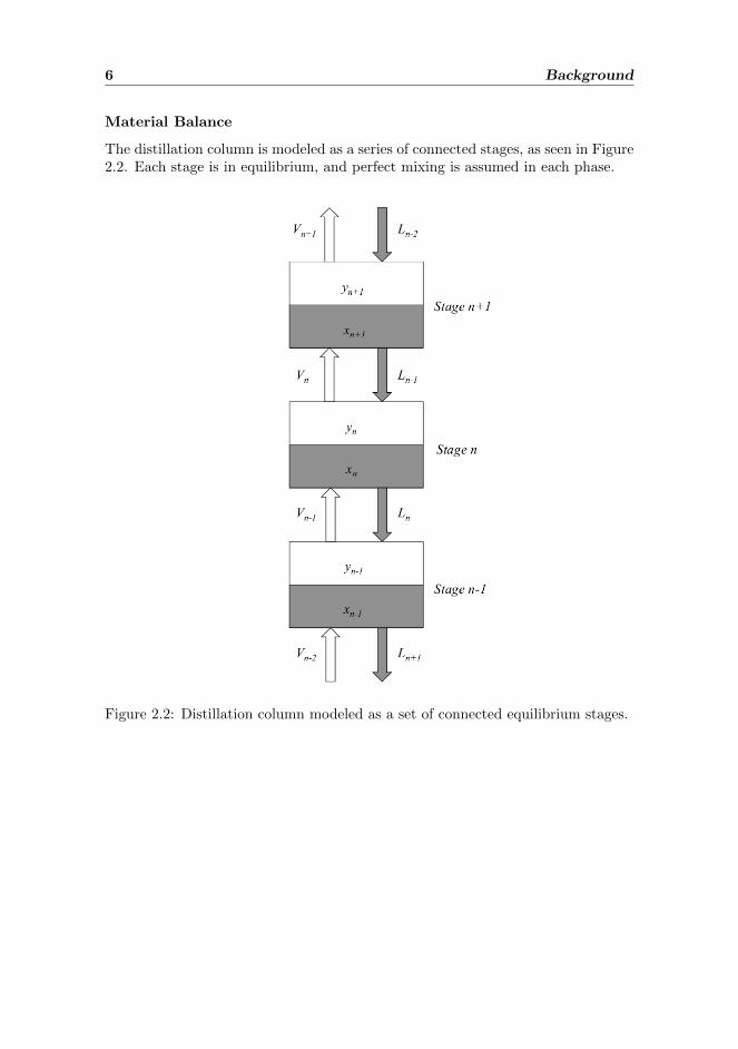
Material Balance

The distillation column is modeled as a series of connected stages, as seen in Figure2.2. Each stage is in equilibrium, and perfect mixing is assumed in each phase.

Figure 2.2: Distillation column modeled as a set of connected equilibrium stages.

2.2. Optimization 7

Based on Figure 2.2 the material balance for component i at stage n is:

dNi,n

dt= (Ln−1xi,n−1 − Vnyi,n)− (Lnxi,n − Vn−1yi,n−1) (2.10)

Here Ni,n is the number of moles of component i at stage n. L and V are the liquidand vapor flow rates. The net material flow, wi, is defined as:

wi,n = Vnyi,n − Ln+1xn+1 (2.11)

For steady – state operation the change Ni,n is zero,dNi,n

dt = 0. Also, the netmaterial flow is constant through the column at steady – state. Equation (2.11)can be rewritten as the equation for the Operating line:

yi,n =Ln+1

Vnxi,n +

1

Vnwi (2.12)

This, together with the VLE – relation, makes it possible to compute all the stagecompositions for the system.

2.2 Optimization

A nonlinear minimization problem is defined as:

minx

J(x, u, d)

subject to ci(x, u, d) = 0 i ∈ Eci(x, u, d) ≤ 0 i ∈ I

(2.13)

J is the cost function, the index set E denotes the equations which are equalityconstraints(the process model) and the set I denotes the indices of the inequalityconstraints. x are the internal variables, u are the manipulated variables and d arethe disturbances.

For a minimization problem as given in Equation (2.13) a cost function is min-imized over the expected disturbances while satisfying the process constraints(Jacobsen 2011). After formulating a model, an optimization algorithm is usedto find a solution. When the solution is found it may be checked by using optimal-ity conditions.

Lagrange multipliers, λ, are introduced as a tool for finding a solution to the op-timization problem. By defining a new function, L, and using λ, the optimizationproblem becomes:

L = J(x, u, d)− λci(x, u, d) (2.14)

8 Background

The solution is characterized by the The Karush – Kuhn – Tucker conditions (ab-breviated KKT – conditions), which are necessary for a first-order solution to beoptimal (Nocedal & Wright 1999). The KKT – conditions are defined:

∇xL(x∗, u∗λ∗) = 0

ci(x∗, u∗) = 0 for all i ∈ E ,

ci(x∗, u∗) ≥ 0 for all i ∈ I,λ∗i ≥ 0 for all i ∈ I,

λ∗i ci(x∗, u∗) = 0 for all i ∈ E ∪ I,

(2.15)

x∗, u∗ and λ∗ are the notations for the variables at the optimal solution.

2.3 Numerical Tools

The different tools used in this work are presented in this section.

2.3.1 Matlab/Simulink

Simulink is an environment in Matlab, used for multidomain simulation and model– based design for dynamic and embedded systems (MathWorks 2012).

2.3.2 Ipopt

The open source software package IPOPT (Interior point optimizer) is an optimiza-tion software for large – scale nonlinear optimization problems. The algorithmis a primal – dual interior point algorithm with a filter line search (Wachter &Biegler 2006).

2.3.3 sIpopt

Optimal Sensitivity Based on Ipopt is a toolbox for Ipopt. This toolbox allow theuser to change parameters of the optimization problem to generate fast solutions(sIpopt Documentation 2012).

2.3.4 AMPL

AMPL – “a mathematical programming language” is a modeling language for solv-ing mathematical problems, typically optimization problems. It was developed anddesigned by Robert Fourer, David M. Gay and Brian W. Kernigham around 1985(Fourer et al. 2003).

An advantage with the syntax of AMPL is its similarity to normal mathemati-cal notation. This thesis uses AMPL as the interface for the solvers Ipopt and

2.4. Self – optimizing Control 9

sIpopt.

2.4 Self – optimizing Control

Optimal operation of chemical plants requires a control structure that drives theeconomic profit to a maximum under varying operating conditions while maintain-ing acceptable operation (Skogestad 2000). According to the time scale in whichthey operate, the control system is usually divided into a hierarchy of several layerswhere the set points of the controlled variables, cs, are the internal variables thatlink the layers together. This is shown in Figure 2.3. The layers include schedul-ing(weeks), site – wide optimization(days), local optimization(hour), supervisorycontrol(minutes) and regulatory control(seconds). The hierarchy functions so thatthe upper layers compute the set points for the layers below.

As previously mentioned, one always wants a system to operate as close to theoptimum as possible. Maximizing the profits is equivalent to minimizing a scalarcost function. The cost function, J , defines the cost for operation. A simple strat-egy to solve this kind of problem is to somehow get the system to self-optimize fordifferent disturbances, instead of doing online optimization for every one. This isthe idea behind Self – optimizing control.

Skogestad gives the following definition for self – optimizing control (Skogestad2000):

“Self – optimizing control is when we can achieve an acceptable losswith constant set point values for the controlled variables (without theneed to reoptimize when disturbances occur).“

10 Background

Scheduling(weeks)

Site-wide optimization(day)

Local optimization(hour)

Supervisorycontrol(minutes)

Regulatorycontrol(seconds)

Controllayer

Fig. 1. Typical control hierarchy in a chemical plant.

performance can be obtained with constant manipu-lated inputs.Self-optimizing control is a direct gener-alization to the case where we can achieve acceptable(economic) performance with constant controlled vari-ables.)

Inspired by the work of Findeisen (e.g. see Findeisenet al. (1980)),Morari et al. (1980) gave a clear descrip-tion ofwhat we here denote self-optimizingcontrol, in-cluding a procedure for selecting controlled variablesbased on evaluating the loss. However, it seems thatnobody, including the authors themselves, has pickedup on the idea. One reason was probably that no goodexample was given in the paper.

More generally, the issue of selecting controlled vari-ables is one of the subtasks in the control structuredesign problem (Foss, 1973); (Morari, 1982); (Skogestadand Postlethwaite, 1996)

(1) Selection of controlled variables (variables withsetpoints )

(2) Selection of manipulated variables(3) Selection of measurements(for control purposes

including stabilization)(4) Selection of a control configuration (structure of

the controller that interconnectsmeasurements &setpoints and manipulated variables)

(5) Selection of controller type (control law specifi-cation, e.g., PID, decoupler, LQG, etc.).

Note that these structural decisions need to be madebefore we can start the actual design the controller. Inmost cases the control structure is designed by a mix-ture between a top-down consideration of control ob-jectives and which degrees of freedom are available tomeet these (tasks 1 and 2), combined with a bottom-updesignof the control system, startingwith the stabiliza-tion of the process (tasks 3,4 and 5). In most practicalcases the problem is solved without the use of any the-oretical tools.

The main objective of this paper is to demonstrate,with a few examples, that the issue of selecting con-trolled variables (task 1) is very important and that theconcept of self-optimizing control provides a usefultool.

2. OPTIMIZATION AND CONTROL

2.1 The optimization problem

The optimizing control problem can be formulated as

(1)

subject to the inequality constraints

(2)

where are the independent variables we can af-fect (degrees of freedom) and are independent vari-ables we can not affect (disturbances). Here the con-straints for instance may be

product specifications (e.g. )manipulated variable saturations (e.g.

)other operational limitation (e.g. avoid flooding)

The analysis in this paper is based on steady-statemod-els and use of constant setpoints at each steady-state(operating point). To analyze the effect of disturbanceswe may time-average various steady-states. The mainjustification for using a steady-state analysis is thatthe economic performance is primarily determined bysteady-state considerations.

If we formulate the optimizing control problem in theusual mathematical fashion as given in (1), then we wefind that a centralized solution is the optimal choice.Here there is one “big” controller, which based on allavailable measurements and other given information(including a model of the system and expected uncer-tainty), computes the optimal values of all manipulatedvariables. Nevertheless, in practice we almost alwaysdecompose the control system intomany separate partsand layers. In the simplest case we may have two lay-ers:

A steady-state optimization layer which computesthe optimal setpoints for the controlled vari-ables, and

Figure 2.3: Typical control hierarchy for a chemical plant (Skogestad &Postlethwaite 2005).

So, the key to deciding a self – optimizing control structure is to find what theseinternal variables should be.

The loss is defined from the previously mentioned cost function as the differencebetween actual operating costs for the controlled system and the optimal opera-tional costs:

L(u, d) = J(u, d)− Jopt(d) (2.16)

L is the loss, J is the actual costs and Jopt is the actual costs at the optimum. Asseen in Equation (2.16), a small difference between J and Jopt is obviously wanted.This is done in practice by using the degrees of freedom for the system to controlthe optimal active constraints and using the remaning degrees of freedom to keepthe self – optimizing variables at a constant setpoint. This method will generallyimpose some loss compared to reoptimization for every disturbance. The aim is tochoose the right variables to control so that the loss is small and acceptable. Figure2.4 illustrates this. Using c1 as a self – optimizing variable results in a smaller loss


than selecting c2 as a self – optimizing variable.

!"#$%&'!( ') '(*'$#+&,- .#"& +,!)# &! '&) !"&'/0/ 122%3#,,45%.#* +%.#667 5- +!(&$!,,'(8 &9# !:#( &#/"#$%&0$#%(* 5%.'(8 &'/# %& &9# )#&"!'(&) 8':#( '( &9# +!!. 5!!.139'+9 '( &9') +%)# ') &9# 22!"&'/';#$66<7=9# '*#% ') >0$&9#$ ',,0)&$%&#* '( ?'8< @A 39#$# 3# )##

&9%& &9#$# ') % ,!)) '> 3# .##" % +!()&%(& )#&"!'(& $%&9#$&9%( $#!"&'/';'(8 39#( % *')&0$5%(+# /!:#) &9# "$!+#))%3%- >$!/ '&) (!/'(%,,- !"&'/%, !"#$%&'(8 "!'(&1*#(!&#* B7< ?!$ &9# +%)# ',,0)&$%&#* '( &9# C80$# '& ')5#&&#$ 13'&9 % )/%,,#$ ,!))7 &! .##" &9# )#&"!'(& !D! +!(4)&%(& &9%( &! .##" !@! +!()&%(&<E( %**'&'!(%, +!(+#$( 3'&9 &9# +!()&%(& )#&"!'(&

"!,'+- ') &9%& &9#$# 3',, %,3%-) 5# %( '/",#/#(&%&'!(#$$!$ "" ! !" !!A #<8< +%0)#* 5- /#%)0$#/#(& #$$!$< =9#'/",#/#(&%&'!( #$$!$ /%- +%0)# % ,%$8# %**'&'!(%, ,!))'> &9# !"&'/0/ )0$>%+# ') 22)9%$"66< =! 5# /!$# )"#+'C+A3# /%-A %) ',,0)&$%&#* '( ?'8< FA *')&'(80')9 5#&3##(&9$## +,%))#) !> "$!5,#/) 39#( '& +!/#) &! &9# %+&0%,'/",#/#(&%&'!(G

1%7 #$%&'()*%+" $,'*-.-/ H( &9# C80$# ') )9!3( &9#+%)# 39#$# &9# /'('/0/ :%,0# !> &9# +!)& 0 ')

!5&%'(#* >!$ ! ! !#$%< H( &9') +%)# &9#$# ') (! ,!))'/"!)#* 5- .##"'(8 % +!()&%(& !! ! !#$%< H(%**'&'!(A '/",#/#(&%&'!( !> %( 22%+&':#66 +!(4)&$%'(& ') 0)0%,,- #%)-A #<8< '& ') #%)- &! .##" %:%,:# +,!)#*<

157 1%!$%&'()*%+" 2)' $,'*-.-/ H( &9') +%)# &9# +!)& ')'()#()'&':# &! :%,0# !> &9# +!(&$!,,#* :%$'%5,# !A%(* '/",#/#(&%&'!( ') %8%'( #%)-<

1+7 1%!$%&'()*%+" &3)(, $,'*-.-/ =9# /!$# *'I+0,&"$!5,#/) >!$ '/",#/#(&%&'!( ') 39#( &9# +!)&1!"#$%&'!(7 ') )#()'&':# &! :%,0# !> &9# +!(&$!,,#*:%$'%5,# !< H( &9') +%)#A 3# 3%(& &! C(* %(!&9#$+!(&$!,,#* :%$'%5,# ! '( 39'+9 &9# !"&'/0/ ')J%&&#$<

=9# ,%&&#$ 0(+!()&$%'(#* "$!5,#/) %$# &9# >!+0) !>&9') "%"#$<

!" #$%&'()* +($,

H()"'$#* 5- &9# 3!$. !> ?'(*#')#( #& %,< KLMA &9# 5%)'+'*#% !> )#,>4!"&'/';'(8 +!(&$!, 3%) >!$/0,%&#* %5!0& @N-#%$) %8! 5- O!$%$' #& %,< KPM< O!$%$' #& %,< KPM 3$'&#&9%& 22'( %&&#/"&'(8 &! )-(&9#)';# % >##*5%+. !"&'/';'(8+!(&$!, )&$0+&0$#A !0$ /%'( !5Q#+&':# ') &! &$%(),%&# &9##+!(!/'+ !5Q#+&':#) '(&! "$!+#)) +!(&$!, !5Q#+&':#)< H(!&9#$ 3!$*)A 4+ 4)%' '$ 5%" ) 6.%!'*$% ! $6 '3+ ,($!+&&7)(*)89+& 43*!3 43+% 3+9" !$%&')%': 9+)"& ).'$-)'*!)99;'$ '3+ $,'*-)9 )"<.&'-+%'& $6 '3+ -)%*,.9)'+" 7)(*=)89+&: )%" 4*'3 *': '3+ $,'*-)9 $,+()'*%> !$%"*'*$%&<K& & &M=9') /#%() &9%& 5- .##"'(8 &9# >0(+&'!( ! .! "# $ %& &9#)#&"!'(& !!A &9$!089 &9# 0)# !> &9# /%('"0,%&#* :%$'%5,#).A >!$ :%$'!0) *')&0$5%(+#) "A '& >!,,!3) 0('R0#,- &9%&&9# "$!+#)) ') !"#$%&'(8 %& &9# !"&'/%, )&#%*-4)&%&#<66 H>3# $#",%+# &9# &#$/ 22!"&'/%, %*Q0)&/#(&)66 5- 22%++#"4&%5,# %*Q0)&/#(&) 1'( &#$/) !> &9# ,!))766 &9#( &9# %5!:#') % "$#+')# *#)+$'"&'!( !> 39%& 3# '( &9') "%"#$ *#(!&# %)#,>4!"&'/';'(8 +!(&$!, )&$0+&0$#< =9# !(,- >%+&!$ &9#->%', &! +!()'*#$ ') &9# #S#+& !> '/",#/#(&%&'!( #$$!$

?'8< F< H/",#/#(&'(8 &9# +!(&$!,,#* :%$'%5,#<

?'8< @< T!)) '/"!)#* 5- .##"'(8 +!()&%(& )#&"!'(& >!$ &9# +!(&$!,,#*:%$'%5,#<

?/ ?@$>+&')" A 0$.(%)9 $6 B($!+&& #$%'($9 CD EFDDDG HIJKLDJ PUV

Figure 2.4: Loss imposed by keeping constant set point for the controlled variable(Skogestad & Postlethwaite 2005).

Different strategies are employed to select good controlled variables. Intuitively, acontrolled variable needs to be insensitive to disturbances at its optimal point sothat the optimum does not shift for disturbances. Also, the optimum should beflat and therefore avoid problems with implementation errors. 4 requirements fora ”good” controllable variables are given in (Skogestad 2000):

• Requirement 1: Its optimal value should be insensitive to disturbances.

• Requirement 2: It should be easy to measure and control accurately.

• Requirement 3: Its value should be sensitive to changes in the manipulatedvariables.

• Requirement 4: For cases with two or more controllable variables, the selectedvariables should not be to closely correlated.

Two methods are used in this work to find these variables: The Minimum Sin-gular Value Rule (Skogestad & Postletwaite 1996) and the Exact Local Method(Halvorsen et al. 2003).

2.4.1 Minimum Singular Value Rule

As mentioned previously the remaining degrees of freedom, after the active con-straints are handled, are used to keep the controlled variables at constant set points.

12 Background

For small deviations around the optimal point it is possible to use a linear rela-tionship between the degrees of freedom, u, and the candidate set of controlledvariables, c:

∆c = G∆u+Gd∆d (2.17)

Here, ∆u = u − uopt and ∆c = c − copt. G is the steady – state gain matrix, andGd the disturbance model. If the disturbances are fixed and G is invertible:

u− uopt = G−1(c− copt) (2.18)

Expressing the cost function in terms of a taylor expansion around the optimalpoint with fixed disturbances results in:

J(u, d) = Jopt(d) +

(∂J

∂u

)T

opt

(u− uopt(d))

+1

2(u− uopt(d))T

(∂2J

∂u2

)opt

(u− uopt(d)) + ....

(2.19)

The higher orders terms are neglected. Notice that the term(∂J∂u

)Topt

= 0 at the

optimum for an unconstrained problem. Equation (2.16) can now be rewritten withthe second – order expansion,

L = J(u, d)− J(uopt(d), d) ≈ 1

2(u− uopt(d))TJuu(u− uopt(d)) (2.20)

where Juu =(

∂2J∂u2

)opt

. By using Equation (2.18), and introducing z = J1/2uu G−1(c−

copt), the equation simplifies:

L =1

2‖z‖22 (2.21)

The notation ‖z‖2 denotes the 2 – norm of the expression. Each controlled vari-able, ci, is assumed to be scaled so that the sum of its optimal range, vi, and itsimplementation error, ni, is unity. The combined errors of the 2 – norm is lessthan 1. The inputs, u, are scaled so that they have the same effect on the cost.This gives a worst – case loss:

max‖c−copt‖261

L =1

2σ2(α1/2G−1) =

α

2

1

σ(G)(2.22)

The constant α = σ is independent of the choice of controlled variables. σ denotesthe minimum singular value. Equation (2.22) then states that one should choosecontrolled variables that maximizes the minimum singular value of the scaled gainmatrix G, from u to c (Skogestad & Postletwaite 1996), (Halvorsen et al. 2003).


2.4.2 Exact Local Method

The Exact Local Method was derived from the Exact Method based on ‘bruteforce” evaluation (Halvorsen et al. 2003). From Halvorsen et al. (2003) z can bewritten,

z = J1/2uu [(J−1uu Jud −G−1Gd)(d− dopt) +G−1n] (2.23)

where n is the implementation error. Notice that the term Jud =(

∂2J∂u∂d

)opt

.

Two positive diagonal matrices, Wd, and W yn are introduced. Wd represents the

expected magnitudes of the individual disturbances. W yn represents the magnitude

of the implementation error for each candidate measurement y. The controlledvariables are a function of the candidate measurements and can linearly be writtenas follows:

∆c = H∆y (2.24)

H is the measurement combination matrix. The expected magnitudes of the dis-turbances can be written:

d− dopt = Wdd′ (2.25)

The disturbance is normalized so that y′ < 1. The implementation error is:

n = HW ynn

y′= Wnn

y′(2.26)

Also ny′

is normalized to have a value of less than 1. More precisely, the combineddisturbances and implementation errors are 2 – norm – bounded:

‖f ′‖2 6 1; f ′ ,

(d′

ny′

)(2.27)

Then the worst – case loss can be formulated as (Halvorsen et al. 2003) :

max‖f ′‖261L = σ(M)2/2 (2.28)

where

M = (Md Mn) (2.29)

Md = J1/2uu (HGy)−1HFWd (2.30)

Mn = J1/2uu (HGy

d)−1HW yn (2.31)

where F = ∂yopt

∂dd is the sensitivity matrix. The average loss (Kariwala, Cao &Janardhanan 2008) is defined:

L =1

2‖M‖2F (2.32)

14 Background

To find the H – matrix that minimize the worst – case loss and average loss, theMinimum loss method is introduced (Alstad, Skogestad & Hori 2009), where H isselected to minimize,

minH‖J1/2

uu (HGy)−1HY ‖F (2.33)

Here, Y = [FWd Wyn ]. The H – matrix which minimizes Equation (2.33) is found

by:

H = GyT (Y Y T )−1 (2.34)

This minimizes both the average loss and worst – case loss (Kariwala et al. 2008).

Chapter 3

Cases

Based on the thesis of Jacobsen (2011), three different case studies were investigatedin this work:

• Case study 1a: One distillation column with constant product prices.

• Case study 1b: One distillation column with purity dependent prices.

• Case study 2: Two distillation columns in sequence with constant productprices.

For each case study the active constraint regions will be identified, drawn and com-pared to previous results (Jacobsen 2011). Each region with unconstrained degreesof freedom will be further investigated to find self – optimizing variables for control.It is assumed that only temperatures and concentrations at the top and bottomstreams are available for control. The Minimum Singular Value rule and the ExactLocal Method is used for this purpose. A selection of the self – optimizing controlstructures were tested using dynamic simulation of the different cases.

The component system were chosen to be:

• Case 1a,b: Toulene and benzene

• Case 2: Toluene, benzene and p – xylene

The temperatures for the binary distillation cases were assumed to depend linearlyon liquid composition (Hori & Skogestad 2007),

Ti = TB,HxHi + TB,Lx

Li (3.1)

where TB,H is the boiling temperature for the heavy component, xHi the mole frac-tion of heavy component, TB,L is the boiling point for the light component and xLiis the mole fraction of the light component.

15

16 Cases

For ternary distillation the relation is assumed to be:

Ti = TB,HxHi + TB,Mx

Mi + TB,Lx

Li (3.2)

Here TB,M is the boiling temperature for middle component and xMi is its molefraction.

3.1 Model

The basis for the case studies is the steady – state model Column A (Morari &Skogestad 1988), with L/V configuration. It has been written in AMPL. Theassumptions for the model are listed in Table 3.1.

Table 3.1: Assumptions for Column A.

Assumptions

1 Constant pressure2 Constant relative volatility3 Equilibrium on all stage4 Total condenser5 Constant molar flows6 No vapor holdup7 Linearized liquid dynamics8 Effect of vapor flow on liquid flow

3.2 Case Study 1a

The first case study is a single distillation column with constant product prices.The column has 41 stages including reboiler where the feed enters at stage 21. Thefeed consists of components A and B, where A is the light component and B is theheavy. Figure 3.1 shows an illustration of a distillation column.

3.2. Case Study 1a 17

F, zF, qF

L

V

D, xD

B, xB

Figure 3.1: Illustration of a single distillation column.

3.2.1 Degrees of Freedom

Assuming that both the pressure and the feed are given, the distillation column hastwo steady – state degrees of freedom (Skogestad, Lundstrom & Jacobsen 1990).There are dynamically four manipulated variables. Two of the four have beenselected to control the levels in the condenser and the reboiler. They have nosteady – state effect. The two degrees of freedom are then selected as the refluxand boilup in the column:

u = [L, V ] (3.3)

3.2.2 Disturbances

The are several disturbances for a distillation process. In this case study, as well asthe other two, only the feed flow rate and energy price are used as disturbances whenmapping the active constraint regions. The intention is to get a good graphicalpresentation of the regions.

d = [F, pV ] (3.4)

Note that when finding the self – optimizing variables, the feed liquid fraction, qF ,and feed composition, zF , are also are included as disturbances.

18 Cases

3.2.3 Optimization Problem

The optimization problem for case 1a is formulated:

minu

J(u, d) = pFF + pV V − pBB − pDD

subject to xB ≥ xB,min

xD ≥ xD,min

V ≤ Vmax

(3.5)

The p – values are the prices for the different flows. The inputs u = [L, V ] and thedisturbances d = [F, pV ].

3.2.4 Constraints

The constraints for a single column with constant prices are purity specific con-straints and capacity constraints:

1. The mole fraction of light component in the distillate should be equal orlarger than a minimum value, xD ≥ xD,min.

2. The mole fraction of heavy component in the bottom should be equal orlarger than a minimum value, xB ≥ xB,min.

3. The boilup should be less or equal to a maximum value, V ≤ Vmax.

Key data needed for the case studies 1a and 1b are given in Table 3.2, The valuesused were taken from Jacobsen (2011).

Table 3.2: Key data for case study 1a and 1b.

Variables Value

αAB 1.5zF 0.5F 0 – 1.6 kmol/minqF 1pF $ 1pV $ 0 – 0.02pD $ 2PB $ 1

xD,min 0.95xB,min 0.99Vmax 4.008 kmol/min

3.3. Case Study 1b 19

3.3 Case Study 1b

Case study 1b is similar to the first. However, now the price of distillate, p′D, isproportional to the purity:

p′D = pDxD (3.6)

The reason for using a variable distillate price is to simulate a case where energyis cheap. With a low energy price it is possible to overpurify the distillate as theprice is proportional to the purity.


The two degrees of freedom are the same the previous case, reflux and boilup inthe column:

u = [L, V ] (3.7)

3.3.2 Disturbances

The disturbances are:

d = [F, pV ] (3.8)


This gives the following optimization problem for case 1b:

minu

J(u, d) = pFF + pV V − pBB − p′DD

subject to xB ≥ xB,min

xD ≥ xD,min

V ≤ Vmax

(3.9)

3.3.4 Constraints

The constraints are the same as for case study 1a:

1. The mole fraction of light component in the distillate should be equal orlarger than a minimum value, xD ≥ xD,min.

2. The mole fraction of the heavy component in the bottom should be equal orlarger than a minimum value, xB ≥ xB,min.

3. The boilup should be less or equal to a maximum value, V ≤ Vmax.

20 Cases

3.4 Case study 2

The model for case study 2 consists of two distillation columns in sequence with aternary component system. The three components are A, B and C, where A is thelightest component, B is the middle one and C is the heavy component. B is themost valuable product. All prices are constant for case study 2. Figure 3.2 showsan illustration of two columns in sequence. The two columns have 41 stages each,with the feed entering column 1 at stage 21, and the bottom product from column1 enters column 2 at stage 21.

F, zF, qF

V1

B1

D1, xA L1 L2

V2

D2, xB

B2, xC

Figure 3.2: Illustration of two distillation columns in sequence.

3.4. Case study 2 21


For the ternary system the distillation column has four steady – state degrees offreedom. Similar to the previous cases the liquid levels in the condensers and reboil-ers are controlled, claiming four out of the eight dynamic manipulated variables.Again, they have no steady – state effect. The remaining four degrees of freedomare selected as:

u = [L1, V 1, L2, V 2] (3.10)

Here, L1 and V 1 are the reflux and boilup for column 1, while L2 and V 2 are thereflux and boilup for column 2.

3.4.2 Disturbances

The disturbances are:

d = [F, pV ] (3.11)


minu

J(u, d) = pFF + pV (V 1 + V 2)− pAD1− pBD2− pCB2

subject to xA ≥ xA,min

xB ≥ xB,min

xC ≥ xC,min

V 1 ≤ V 1max

V 2 ≤ V 2max

(3.12)

3.4.4 Constraints

The constraints for the ternary system is:

1. The mole fraction of component A in the distillate of column 1 should beequal or larger than a minimum value, xA ≥ xA,min.

2. The mole fraction of component B in the distillate of column 2 should beequal or larger than a minimum value, xB ≥ xB,min.

3. The mole fraction of component C in the bottom of column 2 should be equalor larger than a minimum value, xC ≥ xC,min.

22 Cases

4. The boilup of column 1 should be less or equal to a maximum value, V 1 ≤V 1max.

5. The boilup of column 2 should be less or equal to a maximum value, V 2 ≤V 2max.

Key data used in optimization of case study 2 are given in Table 3.3.

Table 3.3: Key data for case study 2.

Variables Value

αAB 1.33αBC 1.5αAC 1.0zF [0.4 0.2 0.4]F 0 – 1.6 kmol/minqF 1pF $ 1pV $ 0 – 0.02pA $ 1PB $ 2PC $ 1

xA,min 0.95xB,min 0.95xC,min 0.95V 1max 4.008 kmol/minV 2max 2.405 kmol/min

Chapter 4

Results

In this chapter the results will be presented. First the maps of the active constraintregions. Second, the results from the Minimum Singular Value Rule and the ExactLocal Method. And last, the testing of a selection of the proposed self – optimizingcontrol structures on the dynamic nonlinear models.

4.1 Active Constraint Regions

For all three case studies, a map of the active constraint regions have been drawnwith regard to the disturbances; feed flow rate and energy prices.

4.1.1 Case Study 1a

In case study 1a, a single distillation column with constant prices, three differentactive constraint regions were found. These regions are sketched in Figure 4.1 andexplained in the bullet points.

• Region I: Only the mole fraction of component A in the distillate, xD, is atits active constraint value. One self – optimizing variable is needed.

• Region II: Both the mole fractions of component A in the distillate, xD,and component B in the bottom, xB , are at their active constraints values.No self – optimizing variables are needed.

• Region III: Both the mole fraction of component A in the distillate, xD,and the boilup, V , are at their respective active constraint values. No self –optimizing variables are needed.

Selected values for each of the regions in Figure 4.1 are presented in Table 4.1. Thehighlighted values represent variables at their active constraint values. It is worthmentioning that in every region the mole fraction of component A in the distillate,xD, is at its active constraint value.

23

24 Results

0 0.2 0.4 0.6 0.8 1 1.2 1.4 1.60

0.002

0.004

0.006

0.008

0.01

0.012

0.014

0.016

0.018

0.02

F

pV

Infeasible

II: xD

, xB

I: xD

III: xD

, Vmax

Figure 4.1: Map of the active constraint regions for a single distillation columnwith constant prices.

4.1.2 Case Study 1b

Case study 1b, a single distillation column with purity dependent prices, gives fiveactive constant regions. These regions are sketched in Figure 4.2. The differentregions are explained in the bullet points.

• Region I: Only the mole fraction of component B in the bottom, xB , is atits active constraint value. One self – optimizing variable is needed.

• Region II: Both the mole fractions of component A in the distillate, xD, andcomponent B in the bottom, xB , are at their respective active constraintsvalues. No self – optimizing variables are need.

• Region III: The mole fraction of component B in the distillate, xB , and theboilup, V , are at their active constraint values. No self – optimizing variablesare need.

• Region IV: The boilup, V , is at its active constraint value. One self –optimizing variable is needed.

• Region V: There are no active constraints. Two self – optimizing variablesare needed.

A selection of optimal values for each region are shown in Table 4.2.

4.1. Active Constraint Regions 25

Table 4.1: Selection of optimal values for a single column constant product prices.

Region I II III

Feed, F 1.2 0.7 1.4price vapor, pV 0.012 0.018 0.002Liquid flow rate, LT 2.7364 1.3275 3.2760Vapor flow rate, VB 3.3631 1.6402 4.008Distillate, D 0.6267 0.3128 0.7320Bottom, B 0.5733 0.2872 0.6680Fraction of light compin distillate, xD

0.95 0.95 0.95

Fraction of heavycomp in bottoms, xB

0.9912 0.99 0.9931

Table 4.2: Selection of optimal values for one column with purity dependent prices.

Region I II III IV V

Feed, F 0.7 0.8 1.4 1.2 0.4Price vapor, pV 0.07 0.12 0.02 0.005 0.01Price distillate, pD 1.9337 1.9000 1.9407 1.9821 1.9823Liquid flow rate, LT 1.6257 1.7700 3.2937 3.4073 1.1402Vapor flow rate, VB 1.9842 2.1870 4.008 4.008 1.3404Distillate, D 0.3585 0.4170 0.7143 0.6007 0.2002Bottom, B 0.3415 0.3830 0.6857 0.5993 0 .1998Fraction of light compin distillate, xD

0.9668 0.95 0.9704 0.9911 0.9912

Fraction of heavycomp in bottoms, xB

0.99 0.99 0.99 0.9922 0.9923

4.1.3 Case Study 2

For the two distillation columns in sequence there are a total of eight active con-straints regions. The regions are sketched in Figure 4.3 and explained in the bulletpoints.

• Region I: Only the mole fraction of component B in the distillate of thesecond column, xB , is at its active constraint value. Three self – optimizingvariables are needed.

• Region II: Both the mole fractions of component A in the distillate of column1, xA, and component B in the distillate of column 2, xB , are at their activeconstraint values. Two self – optimizing variables are needed.

26 Results

0 0.2 0.4 0.6 0.8 1 1.2 1.4 1.60

0.02

0.04

0.06

0.08

0.1

0.12

0.14

F

pV

II: xD

, xB

Infeasible

III: xB, V

max

IV: Vmax

V: No active constraints

I: xB

Figure 4.2: Active constraint regions for a single distillation column with puritydependent prices.

• Region III: The mole fractions of all three components are at their respectiveactive constraint values. One self – optimizing variable is needed.

• Region IV: The mole fraction of component B in the distillate of column2, xB , as well as the boilup for column 1, V 1, are at their active constraintvalues. Two self – optimizing variables are needed.

• Region V: The two mole fractions of component A in the distillate of column1, xA, and component B in the distillate of column 2, xB , and also the boilupof column 1, V 1, are at their active constraint values. One self – optimizingvariables is needed.

• Region VI: All component mole fractions are at their respective active con-straint values along with the boilup of column 1, V 1. No self – optimizingvariables are needed.

• Region VII: The constraint for the mole fraction of component B in thedistillate of column 2, xB , and both the boilup, V 1 and V 2, are active. Oneself – optimizing variable is needed.

• Region VIII: The constraints for the mole fractions of component A incolumn 1, xA, and component B in the distillate of column 2, xB are active.The boilups of column 1 and column 2 , V 1 and V 2, are also active. No self– optimizing variables are needed.

4.1. Active Constraint Regions 27

1.36 1.38 1.4 1.42 1.44 1.46 1.48 1.5 1.520

0.02

0.04

0.06

0.08

0.1

0.12

0.14

0.16

0.18

0.2

F

pV

Infeasible

VIII: xA

, xB,

V1max

, V2max

IV: xB, V1

max

I: xB

II: xA

, xB

III: xA

, xB, x

C

V: xA

, xB, V1

max

VI: xA

, xB,

xC, V1

max

VII: xB, V1

max, V2

max

Figure 4.3: Map of the active constraint regions for two columns in sequence withconstant prices.

In Table 4.3 selected values for the active constraint regions of case study 2 areshown. Also in this case study there is one constraint, xB , which is active for allthe regions.

28 Results

Table 4.3: Selection of optimal values for two columns in sequence with constantprices.

Region I II III IV V VI VII VIII

F 1.36 1.4 1.4 1.36 1.47 1.45 1.46 1.48pV 0.03 0.09 0.16 0.02 0.1 0.2 0.01 0.02LT1 3.3240 3.2860 3.3122 3.4556 3.4001 3.4075 3.4054 3.3965LT2 1.9668 1.7940 1.6777 2.0809 1.9593 1.7642 2.1365 2.1367VB1 3.8810 3.8657 3.89234 4.008 4.008 4.008 4.008 4.008VB2 2.2214 2.0391 1.9111 2.3419 2.2175 2.0058 2.405 2.405D1 0.5570 0.5798 0.5802 0.5524 0.6079 0.6005 0.6026 0.6116D2 0.2546 0.2452 0.2334 0.2610 0.2582 0.2417 0.2685 0.2683B1 0.8030 0.8202 0.8198 0.8076 0.8621 0.8495 0.8574 0.8684B2 0.5484 0.5751 0.5865 0.5467 0.6039 0.6079 0.5888 0.6001xA 0.9594 0.95 0.95 0.9667 0.95 0.95 0.9517 0.95xB 0.95 0.95 0.95 0.95 0.95 0.95 0.95 0.95xc 0.9862 0.9685 0.95 0.9896 0.9697 0.95 0.9867 0.9824J -0.0715 0.2863 0.6952 -0.1340 0.3643 0.96108 -0.2044 -0.1401

4.2 Self – optimizing variables

The scaled gains of the stage temperatures in each region of the three different casestudies were found according to the Minimum Singular Value Rule. The tempera-tures with the largest scaled gains were chosen as self – optimizing variables. TheExact Local Method was used to find combinations of stage temperatures as self –optimizing variables.

The pairing of active constraints and self – optimizing variables with the degreesof freedom, along with the their optimal values for the different case studies, areshown in Appendix B.

4.2.1 Minimum Singular Value Rule

4.2.2 Case Study 1a

As seen in Figure 4.1, only region I has unconstrained degrees of freedom afterthe active constraints are controlled. The reflux, L, was assumed to control theactive constraint, while the boilup, V , was used for self – optimizing control. Apresentation of the scaled gains are given in Figure 4.4. The scaled gain is largestat stage number 11.

4.2. Self – optimizing variables 29

5 10 15 20 25 30 35 400

0.5

1

1.5

2

2.5

3

3.5

4

4.5

5

Stage number

Scale

d g

ain

Figure 4.4: Scaled gains for case study 1a.

4.2.3 Case Study 1b

The three regions I, IV and V in Figure 4.2, have unconstrained degrees of freedomleft after controlling the active constraints. The scaled gains for each region areshown in Figure 4.5

In region I, the boilup, V , was assumed to be controlling the active constraint,while the reflux, L, was used for self – optimizing control. The boilup, V , was atits active constraint value in region IV, which left the reflux, L, for self – optimizingcontrol. The last region, V, has no active constraints. Both the boilup, V , and thereflux L are free for self – optimizing control.

The largest scaled gain in region I is stage 35. In region IV stage 14 has thelargest scaled gain, while the largest scaled gain for region V is at stage 32 for bothperturbations in reflux and boilup.

4.2.4 Case Study 2

There are 6 regions, I, II, III, IV, V and VII, with unconstrained degrees of freedomin case study 2.

In region I the reflux of column 2, L2, was assumed to be controlling the ac-tive constraint, while the reflux of column 1, L1 and the boilups, V 1 and V 2, wereused for self – optimizing control. The scaled gains can be seen in Figure 4.6. Thelargest scaled gain for a perturbation in L1 is at stage 32 in column 1. Stage 13

30 Results

5 10 15 20 25 30 35 400

2

4

6

8

10

12

14

16

Stage number

Scale

d g

ain

(a) Region I.

5 10 15 20 25 30 35 400

50

100

150

200

250

300

Stage number

Scale

d g

ain

(b) Region IV.

5 10 15 20 25 30 35 400

0.5

1

1.5

2

2.5

3

3.5

4

4.5

5

Stage number

Scale

d g

ain

(c) Region V with perturbation in L.

5 10 15 20 25 30 35 400

0.5

1

1.5

2

2.5

3

3.5

4

4.5

5

Stage number

Scale

d g

ain

(d) Region V with perturbation in V .

Figure 4.5: Scaled gains for regions (a) I, (b) IV and (c)(d) V.

in column 1 has the largest scaled gain for a perturbation in V 1, and stage 13 incolumn 2 has the largest gain for a perturbation in V 2.

In region II both refluxes, L1 and L2, are assumed to control the active constraints.The remaining degrees of freedom are the boilups, V 1 and V 2. They are used forself – optimizing control. The scaled gains for this region are shown in Figure 4.7.The largest scaled gain for a perturbation in V 1 is at stage 12 in column 1, and forV 2 at stage 9 in column 2.

In region III, the refluxes, L1 and L2, and the boilup, V 2, are assumed to controlthe active constraints. The reflux, V 1, was used for self – optimizing control. Theresulting scaled gains are shown in Figure 4.8. The largest scaled gain for a per-turbation in V 1 is at stage 13 in column 1.

The reflux of column 2, L2, and boilup of column 1, V 1, control the active con-straints in region IV. This leaves the reflux of column 1, L1, and boilup of column


5 10 15 20 25 30 35 400

1

2

3

4

5

6

7

8

Stage number

Sca

led

ga

in

Column 1

(a) Perturbation in L1.

5 10 15 20 25 30 35 400

1

2

3

4

5

6

Stage number

Sca

led

ga

in

Column 1

(b) Perturbation in V 1.

5 10 15 20 25 30 35 400

2

4

6

8

10

12

Stage number

Scale

d g

ain

Column 2

(c) Perturbation in V 2.

Figure 4.6: Scaled gains for region I

5 10 15 20 25 30 35 400

1

2

3

4

5

6

7

Stage number

Sca

led

ga

in

Column 1

(a) Perturbation in V 1.

5 10 15 20 25 30 35 400

2

4

6

8

10

12

Stage number

Sca

led

ga

in

Column 2

(b) Perturbation in V 2.

Figure 4.7: Scaled gains for region II.

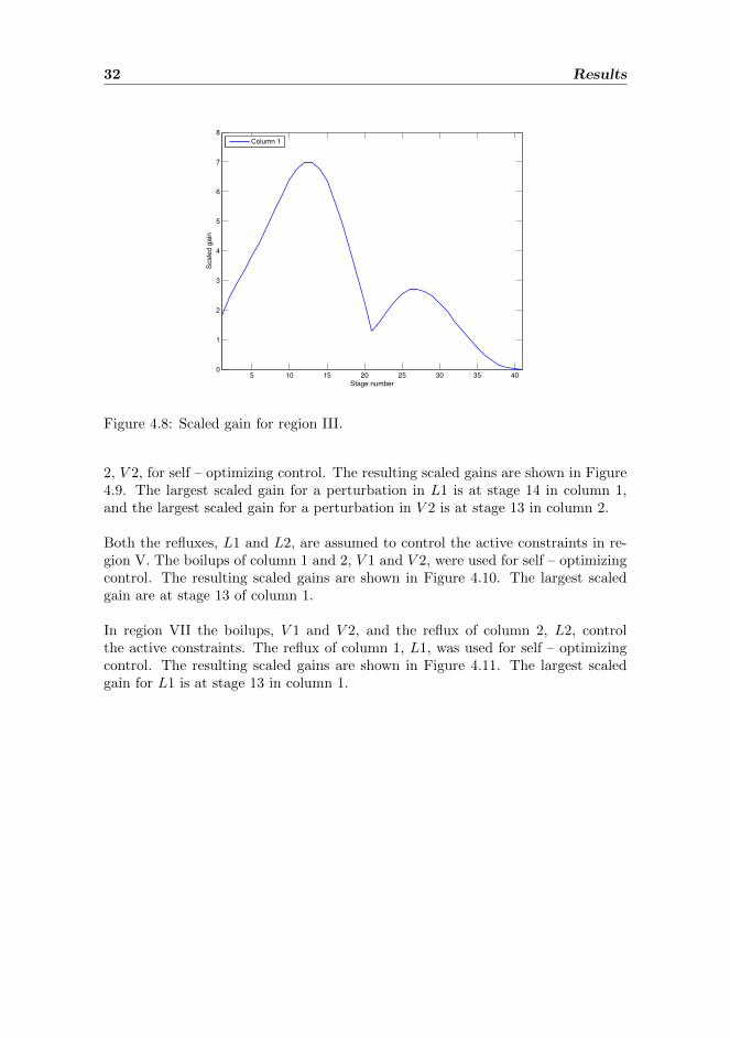
32 Results

5 10 15 20 25 30 35 400

1

2

3

4

5

6

7

8

Stage number

Scale

d g

ain

Column 1

Figure 4.8: Scaled gain for region III.

2, V 2, for self – optimizing control. The resulting scaled gains are shown in Figure4.9. The largest scaled gain for a perturbation in L1 is at stage 14 in column 1,and the largest scaled gain for a perturbation in V 2 is at stage 13 in column 2.

Both the refluxes, L1 and L2, are assumed to control the active constraints in re-gion V. The boilups of column 1 and 2, V 1 and V 2, were used for self – optimizingcontrol. The resulting scaled gains are shown in Figure 4.10. The largest scaledgain are at stage 13 of column 1.

In region VII the boilups, V 1 and V 2, and the reflux of column 2, L2, controlthe active constraints. The reflux of column 1, L1, was used for self – optimizingcontrol. The resulting scaled gains are shown in Figure 4.11. The largest scaledgain for L1 is at stage 13 in column 1.


5 10 15 20 25 30 35 400

50

100

150

200

250

Stage number

Sca

led

ga

in

Column 1

(a) Perturbation L1

5 10 15 20 25 30 35 400

1

2

3

4

5

6

7

8

Stage number

Sca

led

ga

in

Column 2

(b) Perturbation V 2

Figure 4.9: Scaled gains for region IV.

5 10 15 20 25 30 35 400

1

2

3

4

5

6

7

8

Stage number

Scale

d g

ain

Column 2

Figure 4.10: Scaled gain for region V.

34 Results

5 10 15 20 25 30 35 400

50

100

150

200

250

Stage number

Scale

d g

ain

Column 1

Figure 4.11: Scaled gains for region VII.

4.2.5 Exact Local Method

The Exact Local Method was used to find optimal combinations of temperaturesas self – optimizing variables. Both a combination of all temperatures and temper-atures at every 5th stage were considered. In this section only the combinationsof every 5th temperature of case studies 1a and 1b are shown in Table 4.4. Theresults in its entirety are presented in Appendix A.

Table 4.4: Combination of temperatures at every 5th stage as candidate variablesin each region for the case studies 1a and 1b.

Case 1a Case 1b

Region Region Region Region RegionTemperature I I IV V – u = L V – u = V

T5 1 -0.0097 0.3626 1 1T10 2.3889 -0.0875 1 2.7813 2.7635T15 2.6278 -0.2825 0.936 3.8269 3.7548T20 -0.3405 -0.4207 -0.9376 1.0215 0.9085T25 -0.9962 0.0649 0.2764 -2.9444 -2.8345T30 -0.7345 0.8745 0.9513 -4.0572 -3.83T35 -0.2386 1 0.5228 -2.1086 -1.9774T40 0 0.3958 0.1428 -0.5702 -0.5337

4.3. Simulations 35

4.3 Simulations

A selection of the control structures for the different regions for each case studywere tested on the dynamic nonlinear models in Matlab/Simulink. The tested self– optimizing variables were a single stage temperature, a combination of all stagetemperatures and a combination of every 5th stage temperature.

For case studies 1a and b, disturbances occurred at:

• t = 300 min, increase in feed flow rate by 20% .

• t = 700 min, increase in feed composition by 10%.

• t = 1100 min, decrease in liquid composition by 10%.

For case study 2, disturbances occured at:

• t = 200 min, increase in feed flow rate by 0.01 kmol/min.

• t = 400 min, decrease in liquid composition by 10%.

4.3.1 Case Study 1a

The testing of the candidate variables for case study 1a is shown in Figure 4.12.

200 400 600 800 1000 1200 1400

−1.1

−1

−0.9

−0.8

−0.7

−0.6

−0.5

−0.4

−0.3

−0.2

Time[min]

Cost[$]

T

11

Combination of all temperatures

Combination of temperatures in every 5th stage

Figure 4.12: Simulation of region I.

The cost function follows the same trajectory for all the self – optimizing variableswhen controlling them to a constant optimal value.

36 Results

4.3.2 Case Study 1b

The simulation of region I is shown below in Figure 4.13

0 200 400 600 800 1000 1200 1400

−0.5

−0.4

−0.3

−0.2

−0.1

0

0.1

Time[min]

Cost[$]

T

35



Figure 4.13: Simulation of region I.

As seen from the figure, controlling the combinations of temperatures yields ahigher cost than controlling only the temperature at stage 35.

4.3. Simulations 37

The testing of the self – optimizing variables for Region IV are shown in Figure4.14.

50 100 150 200 250 300 350 400−1

−0.9

−0.8

−0.7

−0.6

−0.5

−0.4

−0.3

Time[min]

Cost[$]

T

14



Figure 4.14: Simulation of region IV.

Controlling a combination of temperatures at every 5th stage deals better withincoming disturbances than the other two self – optimizing variables.

4.3.3 Case Study 2

The testing of the self – optimizing variables for regions III and VII are shownin Figure 4.15. The cost functions in both simulations seem to follow the sametrajectory for all the self – optimizing variables.

38 Results

0 100 200 300 400 500 600 7000.55

0.6

0.65

0.7

0.75

0.8

0.85

Time[min]

Cost[$]

T

13



Figure 4.15: Simulation of region III.

0 100 200 300 400 500 600 700−0.4

−0.35

−0.3

−0.25

−0.2

−0.15

−0.1

−0.05

0

Time[min]

Cost[$]

T

13



Figure 4.16: Simulation of region VII.

Chapter 5

Discussion

In this chapter the results and procedures will be explained and discussed.

5.1 Maps of the Active Constraint Regions

The maps of the active constraint regions were found by optimizing the modelswith a sequential increase in the disturbances. The model was solved by settingthe state derivatives equal to zero.

In all regions of case study 1a, xD = xD,min. This follows the Product giveawayrule (Skogestad 2007). A chemical company will not benefit from selling a productwith purity above the required specification when the product price is fixed andover purifying costs extra. Exactly the same is valid for case study 2 and the valu-able product B, xB = xB,min.

There are three active constraint regions in case study 1, mapped in Figure 4.1.By increasing the feed flow rate, the internal flows, L and V , will increase up toa point where V = Vmax. A further increase will violate the purity constraints,thus making the process infeasible. When the energy price is low it is beneficialto over purify the bottom product due to its low value opposed to the distillate.Over purifying the bottom moves more valuable product to the top. Higher energyprices makes this costly and the constraint for the purity of the bottom becomesactive. Also, with higher prices less energy is used to send component A to the topand therefore more feed is needed before the constraint for boilup becomes active.This is seen from the red line between the regions I and III.

There are five active constraint regions in case study 1b. These were mappedin Figure 4.2. As the distillate price is now proportional to purity, the energy priceneeds to be substantially high before the constraint of distillate purity becomesactive. Low energy prices makes it optimal to over purify both the distillate andthe bottom products. Since the the distillate is the most valuable product the bot-

39

40 Discussion

tom product reaches its active constraint value before the distillate. An interestingproperty for this case study is that the constraint for bottom product purity be-comes active when increasing the feed flow rate from region IV to region III. Withthe boilup already being at its maximum, a further increase in the feed flow ratewill activate the bottom product constraint because of the low value of componentB.

Case study 2 gives rise to 8 different active constraint regions. The purity con-straints follow the trends as seen in the two other maps – increasing the energyprice the over purification of distillate and bottom products is too expensive andthe purity constraints become active. With low energy prices, more of componentsA and B are pushed to the top of column 1 and 2, respectively, and the boilupsreaches their active constraint values. The constraint line separating regions II andV has a negative slope. This indicates that the optimal values for the boilup ofcolumn 1 will increase with increasing energy prices. This do not coincide with thetrends seen in the other two cases. However, V 2 is decreasing and also the sumof V 1 + V 2 is decreasing as a counter measure. Another interesting feature is thecurved constraint line for xC separating the regions V and VI. All other purityconstraint lines are horizontal. An increase in the feed while V 1 = V 1max, willmake more of component A flow to column 2, and therefore increasing the amountcomponent C in the bottom of column 2, making the constraint active.

5.1.1 Comparison With Previous Work

3.3. Case studies 45

1.1 1.2 1.3 1.4 1.5 1.60.01

0.012

0.014

0.016

0.018

0.02

F

pV

XB constraint line

Fmax

Vmax constraint line

I: Only XD active

II: XD and Vmax

III: XB and XD

XB, XD and Vmax

IV: Infeasibleregion

Figure 3.2: Active constraint regions for single column with fixed prices(case Ia)

Table 3.2: Single column (case Ia): Values of key variables at selected dis-turbances (F, pV ) (numbers in bold indicate active constraints)

Region(s) I II III

F [mol/s] 1.2 1.4 1.3pV [$/mol] 0.01 0.01 0.015

L [mol/s] 2.827 3.276 2.949V [mol/s] 3.454 4.008 3.627D [mol/s] 0.627 0.731 0.678B [mol/s] 0.573 0.669 0.622xD 0.950 0.950 0.950xB 0.992 0.992 0.990

J [$/s] -0.536 -0.625 -0.566

Figure 5.1: Active constraint region for a single distillation column with constantprices (Jacobsen 2011).

Comparison of the active constraint map for case study 1a constructed in this work

5.1. Maps of the Active Constraint Regions 41

with previous results seen in Figure 5.1 (Jacobsen 2011), shows some differences.The main difference is the line separating the active constraint regions xD – xD, xB .This constraint line is at a larger energy price in this work than in Jacobsen’s. Thereason for this is shown in Jacobsen’s Matlab code, where stage 20 is used for thefeed inlet. This pushes the active constraint line downwards.


0 0.2 0.4 0.6 0.8 1 1.2 1.4 1.6 1.80

0.02

0.04

0.06

0.08

0.1

0.12

0.14

F

pV

XD, XB, VmaxpV,2

pV,1

F1

Fmax

I: No active constraints II: Vmax

III: Vmax, XB

IV: XB

V: XD, XB

VI: Infeasibleregion

Figure 3.4: Single column (case Ib): Active constraint regions with purity-dependent distillate price (p0D = pDxD)

Figure 3.5: Two distillation columns in sequence

Figure 5.2: Active constraint region for a single distillation column with puritydependent prices (Jacobsen 2011).

The active constraint regions for case study 1b in this work and the correspondingby Jacoben (2011), Figure 5.2, are close to equal. The constraint lines separatingregions I and II(actually region IV and V in this work) is curved. This is becauseJacobsen, when drawing the constraint lines, only uses two points, and thereforelacks the curved trends the lines have.

The map for case study 2 in this work and in Jacobsen (2011) seems to be identical,as seen from Figure 5.3.

42 Discussion


1,35 1,4 1.45 1.50

0.02

0.04

0.06

0.08

0.1

0.12

0.14

0.16

0.18

Feed

pV

Infeasibleregion

F1

Fmax

F2

IV: XA, X

B and X

CVII: X

A, X

B,

XC

and V1

III: XB and V

1

I: XB only

pV,1

F3

pV,2

VI: XB, V

1 and V

2

VIII: XA, X

B,

V1 and V

2

II: XA and X

B

V: XA, X

B and V

1

Figure 3.6: Two columns (case II): Active constraint regions

increases with increasing pV , which seems counter-intuitive. However,this is compensated by a decrease in V2 - the sum V1 + V2 is actuallydecreasing, which is what we would expect.

• The next interesting feature about Figure 3.6 is that the border be-tween regions V and VII (part of the green constraint line) is nothorizontal. Across this border, the constraint on xC switches betweenactive and inactive. The reason for this one not being horizontal, is thefollowing: When starting with only the three purity constraints active,an increase in F leads to a proportional increase in all streams, untilthe first capacity constraint becomes active (in this case, this meansV1). Now, since V1 is not allowed to increase further, any extra A fedto the system must either go to stream D1, meaning the constraint onxA is no longer active, or more A goes through to the second columnwhere it enters the distillate stream D2. Thus we need to put moreC into stream B2, thus making the constraint on xC , inactive. Thus,one of two purity constraints must become inactive at this point. Ofcourse, it will become active again once we reach Fmax.

Figure 5.3: Active constraint region for two distillation columns in sequence withconstant prices (Jacobsen 2011).

5.2 Minimum Singular Value Rule

The stage temperatures, with the largest scaled gain for each case study, was cho-sen as self – optimizing variables when using the Minimum Singular Value Rule.This rule generally overestimates the worst – case loss because of the assumptionthat any output deviation satisfying that the combined errors of the 2 – norm isless than 1, is allowed (Halvorsen et al. 2003). This implies that more than thetemperature with the best scaled gain should be further investigated as self – op-timizing variables.

The stage temperatures found in each region of the case studies are concentratedbetween the ends of the column and the feed inlet at stage 21. For most of theregions, the temperature controlled should be put to stages 9 –14 when boilup isthe unconstrained degree of freedom, and stage 30 – 35 when reflux is the un-constrained degree of freedom. The results found coincide with the temperatureprofiles shown in Appendix C.

For two distillation columns in sequence, the concentration of bottom product ofcolumn 1 should rather be used as a controlled variable than using temperatures.Variations in the concentration of the flow that enters column 2 may cause troublesfor column 1, when only controlling the temperatures.

5.3. Simulations 43

5.3 Simulations

Three simulations were done to compare the different control structures in the casestudies 1a and 1b. Two simulations were done for case study 2. Of the five simu-lations, case study 1b, region I, points out. Controlling the temperature in stage35 opposed to controlling combinations of temperatures gives different costs afterthe feed flow rate is increased. The process operates with better profit after distur-bances are introduced by using the temperature at stage 35 as a self – optimizingvariable.

The simulations done in this work is only to demonstrate the applicability of theself – optimizing control structures found. A much more detailed analysis of thedifferent alternatives is needed before choosing the optimal control structures.

5.4 Ipopt/sIpopt

The software package Ipopt/sIpopt was used for optimization of the case studies,and for calculating the optimal sensitivities of the measurements with respect todisturbances. The optimal sensitivities are used in both the Minimum SingularValue Rule and the Exact Local method, thus making Ipopt/sIpopt a useful toolfor self – optimizing control studies.

44 Discussion

Chapter 6

Conclusion

The active constraint regions for each of the three case studies have been identi-fied and mapped with respect to the disturbances; energy price and feed flow rate.Stage temperatures and combinations of stage temperatures have been proposed asself – optimizing variables for the unconstrained degrees of freedom of each region.A selection of the proposed control structures for the different regions of each casestudy have been implemented and compared on the dynamic nonlinear models us-ing Simulink.

It has been shown that the first case study, a single distillation column with con-stant product prices, has 3 active constraint regions. The next case study, a singledistillation column with purity dependent prices, has 5 active constraint regions,while the last case study, two columns in sequence with constant prices, has 8 ac-tive constraint regions.

The optimal sensitivities of the measurements with respect to disturbances, waseasily calculated by using the software package Ipopt/sIpopt.

45

46 Conclusion

Chapter 7

Further Work

The continuation of this work should be to thoroughly test the different self – op-timizing control structures proposed.

One should also test control other variables than only stage temperatures as can-didates for self – optimizing control. I.e. a combination of reflux and temperatureswhich has proved a good alternative (Hori & Skogestad 2007). Other combinationslike flows and flow ratios may also be considered.

In case study 2, an interesting controlled variable to check is the amount of com-ponent A that is carried from column 1 to column 2. Keeping it constant mayremove the problem arising in column 2 when large variations of concentrationflow through it from column 1 (Jacobsen 2011).

47

48 Further Work

Bibliography

Alstad, V., Skogestad, S. & Hori, E. S. (2009), ‘Optimal measurement combinationsas controlled variables’, Journal of Process Control 19, 138 –148.

Cooke, M. & Poole, C. (2000), Encyclopedia of Separation Science, Academic Press.

Fourer, R., Gay, D. M. & Kerninghan, B. (2003), AMPL - A modeling language formathematical programming, second edn, Brooks/Cole Publishing Company /Cengage learning.

Halvorsen, I. J. & Skogestad, S. (2000), Theory of distillation, in ‘Encyclopedia ofSeparation Science’, Academic Press.

Halvorsen, I. J., Skogestad, S., Morud, J. C. & Alstad, V. (2003), ‘Optimal selectionof controlled variables’, Ind. Eng. Chem 42, 3273–3284.

Hori, E. S. & Skogestad, S. (2007), ‘Selection of control structure and temperaturelocation for two-product distillation columns’, Chemical Engineering Researchand Design .

Jacobsen, M. G. (2011), Identifying active constraint regions for optimal operationof process plants, PhD thesis, NTNU.

Kariwala, V., Cao, Y. & Janardhanan, S. (2008), ‘Local self-optimizing controlwith average loss minimization’, In. Eng. Chem. 47, 1150–1158.

MathWorks (2012), Matlab R2012a Documentation, MathWorks.

Morari, M. & Skogestad, S. (1988), ‘Understanding the dynamic behavior of dis-tillation columns’, Ind. and Eng. Chem. Research 27(10), 1848 – 1862.

Nocedal, J. & Wright, S. J. (1999), Numerical Optimization, Springer.

sIpopt Documentation (2012).URL: https://projects.coin-or.org/Ipopt/wiki/sIpopt

Skogestad, S. (2000), ‘Plantwide control: the search for the self-optimizing controlstructure’, Journal of Process Control 10, 487–507.

Skogestad, S. (2007), ‘The do’s and don’ts of distillation column control’, ChemicalEngineering Research and Design pp. 13 – 23.

49

50 BIBLIOGRAPHY

Skogestad, S., Lundstrom, P. & Jacobsen, E. (1990), ‘Selecting the best distillationcontrol figure’, AIChe Journal .

Skogestad, S. & Postlethwaite, I. (2005), Multivariable Feedback Control, 2. edn,John Wiley and Sons Ltd.

Skogestad, S. & Postletwaite, I. (1996), Multivariable Feedback Control, 1. edn,Wiley.

Stichlmair, J. G. & Fair, J. R. (2000), Distillation - Principles and Practice,WILEY-VCH.

Wachter, A. & Biegler, L. T. (2006), ‘On the impementation of a primal - dual in-terior point filter line search algorithm for large-scale nonlinear programming’,Mathematical Programming 106(1), 25–57.

Appendix A

Combinations oftemperatures as self –optimizing variables

The combinations of temperatures as self – optimizing variables (H – matrix) arelisted in the tables below.

Table A.1: Combination of temperatures at every 5th stage as self – optimizingvariables for the case studies 1a and 1b.

Case 1a Case 1b


T5 1 -0.0097 0.3626 1 1T10 2.3889 -0.0875 1 2.7813 2.7635T15 2.6278 -0.2825 0.936 3.8269 3.7548T20 -0.3405 -0.4207 -0.9376 1.0215 0.9085T25 -0.9962 0.0649 0.2764 -2.9444 -2.8345T30 -0.7345 0.8745 0.9513 -4.0572 -3.83T35 -0.2386 1 0.5228 -2.1086 -1.9774T40 0 0.3958 0.1428 -0.5702 -0.5337

51

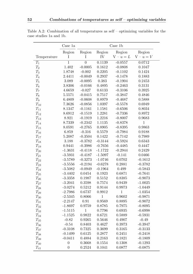
52 Combinations of temperatures as self – optimizing variables

Table A.2: Combination of all temperatures as self – optimizing variables for thecase studies 1a and 1b.

Case 1a Case 1b


T1 1 0 0.1139 -0.0557 0.0712T2 1.402 -0.0005 0.1612 -0.0808 0.1047T3 1.8748 -0.002 0.2205 -0.1102 0.1424T4 2.4411 -0.0049 0.2937 -0.1478 0.1883T5 3.089 -0.0095 0.383 -0.1904 0.2453T6 3.8306 -0.0166 0.4895 -0.2463 0.3131T7 4.6659 -0.027 0.6133 -0.3106 0.3925T8 5.5571 -0.0415 0.7517 -0.3847 0.4846T9 6.4809 -0.0608 0.8979 -0.4687 0.5888T10 7.3626 -0.0856 1.0397 -0.5578 0.6949T11 8.1347 -0.1161 1.1581 -0.6506 0.8034T12 8.6912 -0.1519 1.2281 -0.7336 0.8972T13 8.921 -0.1919 1.2216 -0.8007 0.9683T14 8.7339 -0.2342 1.1135 -0.8378 1T15 8.0591 -0.2765 0.8905 -0.8395 0.9863T16 6.859 -0.316 0.5579 -0.7984 0.9188T17 5.2087 -0.3504 0.1422 -0.7142 0.7989T18 3.188 -0.3782 -0.3144 -0.5924 0.6343T19 0.9441 -0.3986 -0.7656 -0.4485 0.4447T20 -1.3631 -0.4118 -1.1722 -0.2944 0.2429T21 -3.5931 -0.4187 -1.5097 -0.141 0.0466T22 -3.5789 -0.3273 -1.0746 0.0702 -0.1612T23 -3.5556 -0.2194 -0.6278 0.2881 -0.3782T24 -3.5082 -0.0949 -0.1964 0.499 -0.5843T25 -3.4402 0.0454 0.1923 0.6871 -0.7641T26 -3.3358 0.1987 0.5152 0.8385 -0.9073T27 -3.2041 0.3598 0.7574 0.9439 -1.0025T28 -3.0274 0.5212 0.9144 0.9973 -1.0449T29 -2.7986 0.6737 0.9912 1 -1.0354T30 -2.5345 0.8066 1 0.9602 -0.9871T31 -2.2147 0.91 0.9569 0.8895 -0.9072T32 -1.8697 0.9759 0.8785 0.7975 -0.8095T33 -1.5115 1 0.7796 0.6935 -0.6998T34 -1.1525 0.9822 0.6721 0.5889 -0.5931T35 -0.82 0.9265 0.5646 0.4907 -0.49T36 -0.54 0.8403 0.4627 0.3973 -0.3947T37 -0.3108 0.7325 0.3699 0.3165 -0.3133T38 -0.1499 0.6125 0.2877 0.2451 -0.2418T39 -0.0411 0.4884 0.2163 0.1821 -0.1809T40 0 0.3668 0.1554 0.1308 -0.1293T41 0 0.2524 0.1041 0.0877 -0.0875

53

Table A.3: Combination of every 5th temperature as self – optimizing variablesthe for regions I and II, case study 2.

Region I Region II

Temp u = L1 u = V 1 u = V 2 u = V 1 u = V 2

T5 1 1 1 1 1T10 2.1653 2.1568 1.8566 1.8025 1.3151T15 1.9204 1.9167 1.7784 1.7157 0.8019T20 -0.7542 -0.7341 0.3197 -0.1634 0.0291T25 -1.6187 -1.5548 -3.6481 0.2227 -0.809T30 -2.1064 -2.0222 -6.5365 0.3615 -1.2955T35 -2.0223 -1.9523 -3.5676 0.1116 -0.694T40 -1.0273 -0.9931 -1.3053 -0.0005 -0.2543


Table A.4: Combination of all temperatures as self – optimizing variables for theregions I and II, case study 2.

I Region II

Temp u = L1 u = V 1 u = V 2 u = V 1 u = V 2

T1 1 1 1 1 1T2 1.3294 1.3376 1.3219 1.2282 1.3342T3 1.5653 1.5783 1.5406 1.4198 1.6715T4 1.763 1.7726 1.713 1.5919 1.9991T5 1.9724 1.9748 1.8914 1.7598 2.301T6 2.2251 2.2376 2.1185 1.9329 2.5601T7 2.5464 2.5486 2.4002 2.1108 2.7587T8 2.9025 2.907 2.7122 2.2865 2.88T9 3.259 3.266 3.0314 2.4424 2.9147T10 3.5658 3.5721 3.3043 2.5581 2.855T11 3.7804 3.7852 3.4856 2.6142 2.7033T12 3.8446 3.8508 3.5279 2.5916 2.4648T13 3.7052 3.7112 3.3995 2.476 2.1555T14 3.3748 3.3777 3.0754 2.2613 1.7903T15 2.8346 2.8395 2.5646 1.9465 1.3903T16 2.1033 2.0989 1.8785 1.5422 0.971T17 1.2183 1.2203 1.0582 1.0627 0.5496T18 0.2289 0.2272 0.141 0.5306 0.1376T19 -0.804 -0.8084 -0.8185 -0.0334 -0.2531T20 -1.8499 -1.8578 -1.7727 -0.6069 -0.6208T21 -2.8486 -2.8572 -2.6986 -1.1726 -0.9625T22 -2.5416 -2.5409 -2.2509 -0.9075 -1.6052T23 -2.1314 -2.1253 -1.7436 -0.8127 -2.3437T24 -1.7464 -1.7371 -1.2831 -0.8813 -3.1457T25 -1.4614 -1.4448 -0.9238 -1.0694 -3.9635T26 -1.2759 -1.2564 -0.6837 -1.3123 -4.7246T27 -1.1883 -1.1676 -0.5474 -1.5381 -5.3483T28 -1.1681 -1.1498 -0.4901 -1.6806 -5.7606T29 -1.197 -1.1722 -0.4861 -1.6967 -5.9108T30 -1.2403 -1.2116 -0.5094 -1.5684 -5.7923T31 -1.2816 -1.2544 -0.5456 -1.3132 -5.4372T32 -1.3151 -1.2883 -0.5827 -0.9728 -4.91T33 -1.3152 -1.2895 -0.6075 -0.5986 -4.2835T34 -1.2858 -1.2684 -0.6201 -0.2416 -3.6297T35 -1.2345 -1.2156 -0.6097 0.06 -3.0039T36 -1.1564 -1.132 -0.5866 0.2836 -2.4403T37 -1.0439 -1.0308 -0.5473 0.4186 -1.9638T38 -0.9194 -0.9079 -0.4953 0.4657 -1.577T39 -0.7863 -0.7717 -0.4257 0.431 -1.2841T40 -0.6422 -0.633 -0.3493 0.3227 -1.0824T41 -0.4907 -0.4859 -0.2676 0.1515 -0.9707

55

Table A.5: Combination of every 5th temperature as self – optimizing variables forthe regions III, IV, V and VII, case study 2.

Region III Region IV Region V Region VII

Temp u = V 1 u = L1 u = V 2 u = V 2 u = L1

T5 1 1 1 1 1T10 1.8437 1.8885 2.0303 1.431 1.8675T15 1.8224 1.8781 2.2291 0.9918 2.0853T20 -0.1336 -0.2186 0.7461 0.1803 1.2389T25 0.2778 -0.2828 -1.0365 -0.4353 1.215T30 0.4077 -0.2485 -2.1143 -0.6829 0.9381T35 0.1252 -0.3205 -1.1058 -0.3383 0.4987T40 -0.0011 -0.1745 -0.4249 -0.123 0.1782


Table A.6: Combination of all temperatures as a self – optimizing variables for theregions III, IV, V and VII, case study 2.

Region III Region IV Region V Region VII

Temp u = V 1 u = L1 u = V 2 u = V 2 u = L1

T1 1 1 1 1 1T2 1.2728 1.2493 1.1626 1.246 1.3896T3 1.4311 1.3732 1.2755 1.4896 1.7624T4 1.5364 1.4342 1.3877 1.7218 2.1329T5 1.6464 1.4997 1.4702 1.9214 2.52T6 1.8022 1.6168 1.5627 2.0605 2.9352T7 2.0203 1.8036 1.6546 2.1106 3.3775T8 2.2863 2.0519 1.7561 2.0491 3.8313T9 2.5707 2.334 1.8538 1.8629 4.2695T10 2.8322 2.6104 1.9469 1.554 4.6574T11 3.0258 2.8357 1.9892 1.1409 4.9572T12 3.1027 2.9642 1.9939 0.6554 5.1341T13 3.0301 2.9551 1.9378 0.138 5.1612T14 2.779 2.7785 1.7946 -0.368 5.0247T15 2.3464 2.4194 1.5686 -0.823 4.7251T16 1.7417 1.8805 1.2466 -1.1991 4.2786T17 0.9922 1.1815 0.8334 -1.4819 3.7141T18 0.1356 0.3567 0.3415 -1.6681 3.0666T19 -0.7816 -0.5513 -0.2076 -1.7676 2.3747T20 -1.7144 -1.4972 -0.7928 -1.7966 1.6731T21 -2.6261 -2.439 -1.4155 -1.7735 0.9915T22 -2.0481 -2.1213 -1.077 -1.2108 1.2106T23 -1.4207 -1.6802 -1.037 -0.6266 1.4137T24 -0.8525 -1.2371 -1.2402 -0.0449 1.558T25 -0.395 -0.8624 -1.5995 0.5009 1.6255T26 -0.0636 -0.5799 -1.999 0.9705 1.6169T27 0.1526 -0.3837 -2.3159 1.3261 1.5438T28 0.2784 -0.255 -2.466 1.5451 1.4217T29 0.3345 -0.1737 -2.3864 1.6264 1.266T30 0.3435 -0.123 -2.0887 1.5917 1.0918T31 0.3213 -0.0904 -1.5955 1.4773 0.9111T32 0.2776 -0.0686 -1.0083 1.3203 0.7342T33 0.2266 -0.0532 -0.4002 1.1539 0.5693T34 0.1747 -0.0416 0.161 0.9982 0.422T35 0.1252 -0.0325 0.6004 0.8628 0.2963T36 0.0812 -0.0254 0.8937 0.7493 0.1938T37 0.0477 -0.019 1.0429 0.6539 0.1153T38 0.022 -0.0126 1.0626 0.5733 0.0591T39 0.0066 -0.0048 0.9438 0.5031 0.0234T40 -0.002 0.005 0.7356 0.4427 0.0057T41 -0.001 0.0178 0.4384 0.3948 0.0032

Appendix B

Pairing

The pairing of the active constraints and self – optimizing variables with the degreesof freedom are shown in the tables below. The optimal values of the variables arealso listed.

B.1 Case study 1a

Table B.1: Pairing of active constraints/self – optimizing variables with degrees offreedom, case study 1a.

Active constraints/self – optimizing variables

DOF fixed values

xD L 0.95T11 V 380.197 [◦C]Comb all V 2.093e+04 [◦C]Comb 5th V 1.433e+03 [◦C]

57

58 Pairing

B.2 Case study 1b

Table B.2: Region I, case study 1b.


DOF fixed values

xB V 0.99T35 L 358.582 [◦C]Comb all L 2.311e+03 [◦C]Comb 5th L 542.155 [◦C]

Table B.3: Region IV, case study 1b.


DOF fixed values

Vmax V 4.008 [kmol/min]T35 L 353.466 [◦C]Comb all L 4.798e+03 [◦C]Comb 5th L 51.579e+03 [◦C]

Table B.4: Region V, case study 1b.


DOF fixed values

T32 L 356.868 [◦C]Comb all L 443.092 [◦C]Comb 5th L -222.039 [◦C]

T32 V 356.868 [◦C]Comb all V -995.682 [◦C]Comb 5th V -116.635 [◦C]

B.3. Case study 2 59

B.3 Case study 2

Table B.5: Region I, case study 2.


DOF fixed values

xB L2 0.95

Column 1T32 L1 359.619 [◦C]Comb all L1 5.466e+03 [◦C]Comb 5th L1 -760.788 [◦C]

T30 V 1 361.219 [◦C]Comb all V 1 5.614e+03 [◦C]Comb 5th V 1 -666.933 [◦C]

Column 2T30 V 2 391.589 [◦C]Comb all V 2 7.948e+03 [◦C]Comb 5th V 2 -3.873e+03 [◦C]

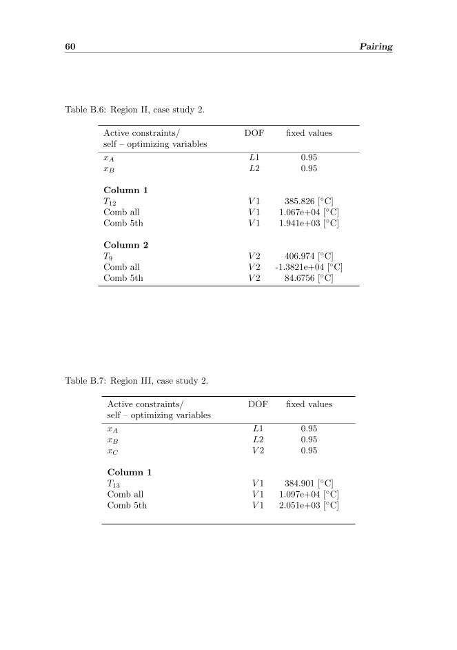
60 Pairing

Table B.6: Region II, case study 2.


DOF fixed values

xA L1 0.95xB L2 0.95

Column 1T12 V 1 385.826 [◦C]Comb all V 1 1.067e+04 [◦C]Comb 5th V 1 1.941e+03 [◦C]

Column 2T9 V 2 406.974 [◦C]Comb all V 2 -1.3821e+04 [◦C]Comb 5th V 2 84.6756 [◦C]

Table B.7: Region III, case study 2.


DOF fixed values

xA L1 0.95xB L2 0.95xC V 2 0.95

Column 1T13 V 1 384.901 [◦C]Comb all V 1 1.097e+04 [◦C]Comb 5th V 1 2.051e+03 [◦C]

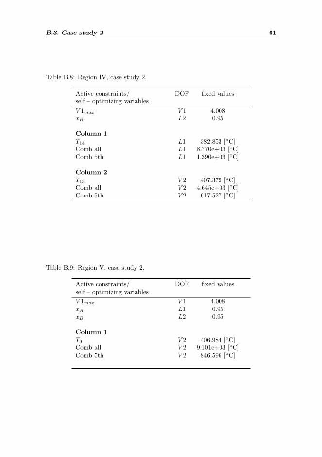
B.3. Case study 2 61

Table B.8: Region IV, case study 2.


DOF fixed values

V 1max V 1 4.008xB L2 0.95

Column 1T14 L1 382.853 [◦C]Comb all L1 8.770e+03 [◦C]Comb 5th L1 1.390e+03 [◦C]

Column 2T13 V 2 407.379 [◦C]Comb all V 2 4.645e+03 [◦C]Comb 5th V 2 617.527 [◦C]

Table B.9: Region V, case study 2.


DOF fixed values

V 1max V 1 4.008xA L1 0.95xB L2 0.95

Column 1T9 V 2 406.984 [◦C]Comb all V 2 9.101e+03 [◦C]Comb 5th V 2 846.596 [◦C]

62 Pairing

Table B.10: Region VII, case study 2.


DOF fixed values

V 1max V 1 4.008V 2max V 2 0.95xB L2 0.95

Column 1T13 L1 384.021 [◦C]Comb all L1 3.249e+04 [◦C]Comb 5th L1 3.407e+03 [◦C]

Appendix C

Temperature profiles

C.1 Case 1a

Temperature profiles of the distillation column in the different active constraintregions.

0 5 10 15 20 25 30 35 40355

360

365

370

375

380

Stage number

Tem

pera

ture

Nominal

∆ VB = +0.1

Figure C.1: Temperatureprofile of region I.

63

64 Temperature profiles

C.2 Case 1b

Temperature profiles of the distillation column for the different regions.

0 5 10 15 20 25 30 35 40355

360

365

370

375

380

Stage number

Te

mp

era

ture

Nominal

∆ LT = +0.01

(a) Regin I

0 5 10 15 20 25 30 35 40

355

360

365

370

375

380

Stage number

Te

mp

era

ture

Nominal

∆ LT = −0.01

(b) Region IV

0 5 10 15 20 25 30 35 40

355

360

365

370

375

380

Stage number

Tem

pera

ture

Nominal

∆ LT = +0.01

∆ VB = +0.01

(c) Region V

Figure C.2: Temperature profiles for case study 1b.

C.3. Case 2 65

C.3 Case 2

Temperature profiles of the two distillation columns in sequence for the differentregions.

5 10 15 20 25 30 35 40

355

360

365

370

375

380

385

390

395

400

Stage number

Te

mp

era

ture

Nominal

∆ LT1 = + 0.1

(a) Column 1

5 10 15 20 25 30 35 40

385

390

395

400

405

410

Stage number

Te

mp

era

ture

Nominal

∆ VB1 = + 0.1

∆ VB2 = + 0.1

(b) Column 2

Figure C.3: Temperature profiles for region I.

5 10 15 20 25 30 35 40

355

360

365

370

375

380

385

390

395

400

Stage number

Te

mp

era

ture

Nominal

∆ VB1 = + 0.1

(a) Column 1

5 10 15 20 25 30 35 40

385

390

395

400

405

410

Stage number

Te

mp

era

ture

Nominal

∆ VB2 = + 0.1

(b) Column 2

Figure C.4: Temperature profiles for region II.


5 10 15 20 25 30 35 40

355

360

365

370

375

380

385

390

395

400

Stage number

Tem

pera

ture

Nominal

∆ VB1 = + 0.1

Figure C.5: Temperatureprofile of region III.

5 10 15 20 25 30 35 40

355

360

365

370

375

380

385

390

395

400

Stage number

Te

mp

era

ture

Nominal

∆ LT1 = − 0.01

(a) Column 1

5 10 15 20 25 30 35 40

385

390

395

400

405

410

Stage number

Te

mp

era

ture

Nominal

∆ VB2 = − 0.1

(b) Column 2

Figure C.6: Temperature profiles for region IV.

C.3. Case 2 67

5 10 15 20 25 30 35 40

385

390

395

400

405

410

Stage number

Te

mp

era

ture

Nominal

∆ VB2 = − 0.07

Figure C.7: Temperatureprofile of region V.

5 10 15 20 25 30 35 40

355

360

365

370

375

380

385

390

395

400

Stage number

Te

mp

era

ture

Nominal

∆ LT1 = + 0.003

Figure C.8: Temperatureprofile of region VII.

Appendix D

AMPL code

The AMPL code for the run file and distillation model of case studies 1a and 1bare shown in below.

##################################################

# Optimization of a distillation column with

# parameters Energy price, pV, and feed rate, F.

##################################################

#--------------------------------------------

# Setting parameters as variables

#--------------------------------------------

var F ; # feed

var zF ; # feed composition

var qF ; # feed liquid composition

var pV ; # price vapor($)

#----------------------

# PARAMETERS

#----------------------

param NT, := 41 ; # number of stages including reboiler

param NF, := 21 ; # location of of feed stage (counted from the bottom)

### P-Controllers for control of reboiler and condenser hold up

param KcB, := 10 ; # controller gain reboiler

param KcD, := 10 ; # controller gain condenser

param MDs, := 0.5 ; # nominal holdup condenser

param MBs, := 0.5 ; # nominal holdup reboiler

param Ds, := 0.5 ; # nominal flow condenser

param Bs, := 0.5 ; # nominal flow reboiler

param alpha, := 1.5 ; # relative volatility

69

70 AMPL code

param M0, := 0.5 ; #nominal liquid holdups

### Data for linearized liquid flow dynamics

# (does not apply to reboiler or condenser)

param tau1, := 0.063; # time constant for lquid dynamics (min)

param F0, := 1 ; # nominal feed rate (kmol/min)

param qF0, := 1 ; # nominal fraction of liquid

param L0, := 2.70629 ; # nominal reflux flow (from steady-state data)

param L0b, >= 0 ; # nominal liquid flow below flow (kmol/min)

param lambda, := 0 ; # effect of vapor flow on liquid flow ("K2-effect")

param V0, := 3.20629 ; # nominal vapor flow

param V0t, >= 0 ; # nominal vapor flow

### Define prices

param pF, := 1 ; # feed price ($)

param pB, := 1 ; # bottoms price ($)

param pD, := 2 ; # price distillate ($)

#---------------------------------

# VARAIBLES

#---------------------------------

var LT >= 0.1 <= 10 := 2.76969 ;

var VB >= 0.1 <= 10 := 3.39585 ;

var L {2..NT} >= 0 ;

var V {1..NT-1} >= 0 ;

var D >= 0 ; # distillate flow

var B >= 0 ; # bottoms flow

var MB >= 0 ; # actual reboiler holdup

var MD >= 0 ; # actual condenser holdup

var x {1..2*NT} >= 0 ;

var y {1..NT-1} >= 0 ;

#----------------------------------------------------------------------------------

# Initial values for stages/holdup and distillate and bottom flow

#----------------------------------------------------------------------------------

for {i in 1..2*NT}

let x[i] := 0.5 ; # initial values for composition in the stages

let L0b := L0 + qF0*F0 ;

let V0t := V0 + (1 - qF0)*F0 ;

#-----------------------

# CONSTRAINTS

71

#-----------------------

### Control liquid level in reboiler and condenser

const1:

MB = x[NT+1] ;

const2:

MD = x[2*NT] ;

const3:

B = Bs + (MB - MBs)*KcB ;

const4:

D = Ds + (MD - MDs)*KcD ;

### Model

const5 {i in 1..NT-1}:

y[i] = alpha*x[i]/(1 + (alpha-1)*x[i]); # vapor-liquid equilibria

const6 {i in 1..NF-1}:

V[i] = VB ; # vapor flow below feed

const7 {i in NF..NT-1}:

V[i] = VB + (1-qF)*F ; # vapor flow above feed

const8 {i in 2..NF}: # liquid flow below feed

L[i] = L0b + (x[i+NT] - M0)/tau1 + lambda*(V[i-1] - V0) ;

const9 {i in NF+1..NT-1}: # liquid flow above feed

L[i] = L0 + (x[i+NT] - M0)/tau1 + lambda*(V[i-1] - V0t) ;

const10:

L[NT] = LT ; # liquid flow condenser


L[i+1] - L[i] + V[i-1] - V[i] = 0 ; # dMdt below feed


L[i+1]*x[i+1] - L[i]*x[i] + V[i-1]*y[i-1]

- V[i]*y[i] = 0 ; # dMxdt above feed

const13 {i in NF+1..NT-1}:

L[i+1] - L[i] + V[i-1] - V[i] = 0 ; # dMdt above feed


L[i+1]*x[i+1] - L[i]*x[i] + V[i-1]*y[i-1]

- V[i]*y[i] = 0 ; # dMxdt above feed

const15:

L[2] - V[1] - B = 0 ; # dMdt reboiler

const16:

72 AMPL code

L[2]*x[2] - V[1]*y[1] - B*x[1] = 0 ; # dMxdt reboiler

const17:

L[NF+1] - L[NF] + V[NF-1] - V[NF] + F = 0 ; # dMdt feed

const18:

L[NF+1]*x[NF+1] - L[NF]*x[NF] + V[NF-1]*y[NF-1]

- V[NF]*y[NF] + F*zF = 0 ; # dMxdt feed

const19:

V[NT-1] - LT - D = 0 ; # dMdt condenser

const20:

V[NT-1]*y[NT-1] - LT*x[NT] - D*x[NT] = 0 ;# dMxdt condenser

### Inequality constraints

const21:

1 - x[1] >= 0.99 ; # fraction of heavy comp in bottom

const22:

x[NT] >= 0.95 ; # fraction of light comp in distillate

const23:

VB <= 4.008 ; # max vapor flow

### Initial constraints for parameters

constF: F = nominal_F ;

constpV: pV = nominal_pV ;

constzF: zF = nominal_zF ;

constqF: qF = nominal_qF ;

#--------------------

# OBJECTIVE FUNCTION

#--------------------

minimize cost: pF*F + pV*VB - pB*B - pD*D ;

73

The AMPL code for the run file and distillation model of case study 2 are shownbelow.

#############

# RUN FILE #

#############

reset ;

#----------------------

# Set parameters

#---------------------

param nominal_F := 1.35 ;

param d1_perturbed_F := 1.35 ;



param nominal_pV := 0.03 ;

param d1_perturbed_pV := 0.03 ;

param d2_perturbed_pV := 0.03 ;

param d3_perturbed_pV := 0.03;

# param nominal_zF := 0.5 ;

# param d1_perturbed_zF := 0.5 ;




param nominal_qF := 1 ;

param d1_perturbed_qF := 1 ;



#--------------------------------------------

# Declare suffixes for sIpopt code

#--------------------------------------------

# enumerate parameters that will be perturbed

suffix sens_state_0, IN ;

# enumerate parameters that will be perturbed and also indicate the

# order for parameters at the perturbed value


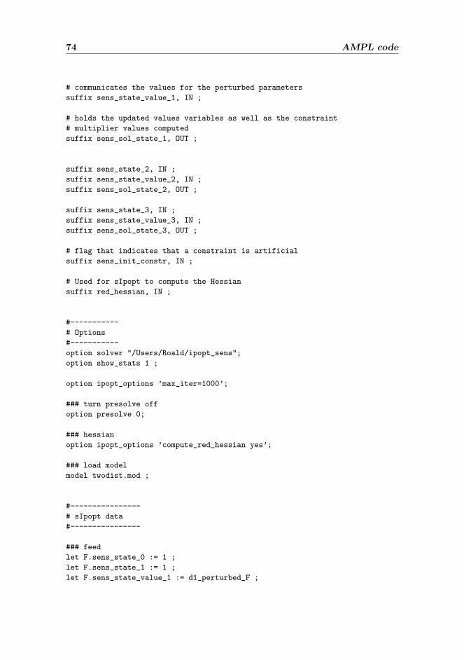
74 AMPL code

# communicates the values for the perturbed parameters

suffix sens_state_value_1, IN ;

# holds the updated values variables as well as the constraint

# multiplier values computed

suffix sens_sol_state_1, OUT ;







# flag that indicates that a constraint is artificial

suffix sens_init_constr, IN ;

# Used for sIpopt to compute the Hessian

suffix red_hessian, IN ;

#-----------

# Options

#-----------

option solver "/Users/Roald/ipopt_sens";

option show_stats 1 ;

option ipopt_options ’max_iter=1000’;

### turn presolve off

option presolve 0;

### hessian

option ipopt_options ’compute_red_hessian yes’;

### load model

model twodist.mod ;

#----------------

# sIpopt data

#----------------

### feed

let F.sens_state_0 := 1 ;

let F.sens_state_1 := 1 ;

let F.sens_state_value_1 := d1_perturbed_F ;

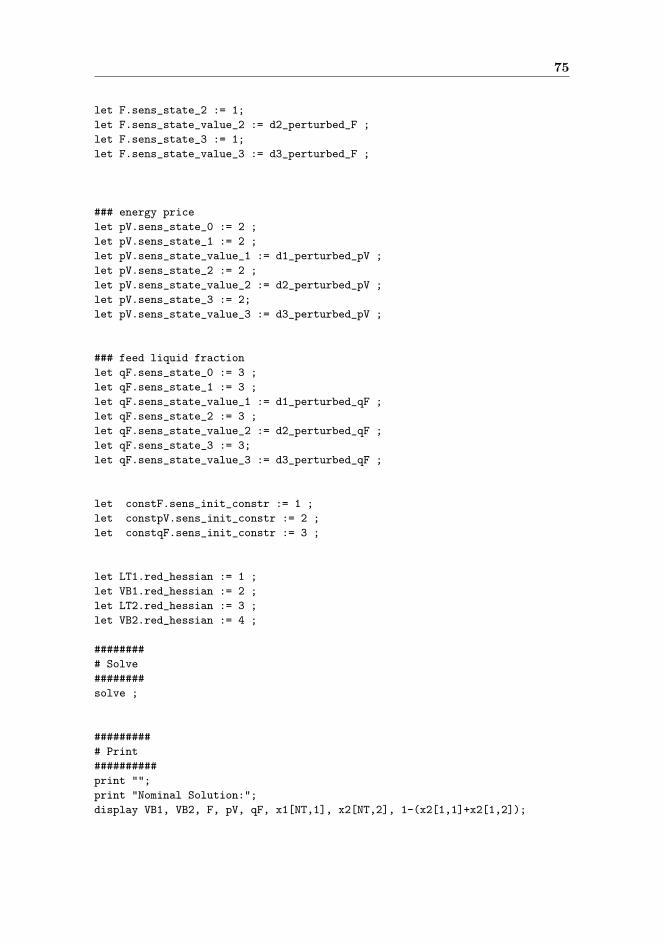
75

let F.sens_state_2 := 1;


let F.sens_state_3 := 1;


### energy price

let pV.sens_state_0 := 2 ;


let pV.sens_state_value_1 := d1_perturbed_pV ;



let pV.sens_state_3 := 2;


### feed liquid fraction

let qF.sens_state_0 := 3 ;


let qF.sens_state_value_1 := d1_perturbed_qF ;



let qF.sens_state_3 := 3;


let constF.sens_init_constr := 1 ;

let constpV.sens_init_constr := 2 ;

let constqF.sens_init_constr := 3 ;

let LT1.red_hessian := 1 ;

let VB1.red_hessian := 2 ;

let LT2.red_hessian := 3 ;

let VB2.red_hessian := 4 ;

########

# Solve

########

solve ;

#########

# Print

##########

print "";

print "Nominal Solution:";

display VB1, VB2, F, pV, qF, x1[NT,1], x2[NT,2], 1-(x2[1,1]+x2[1,2]);

76 AMPL code

print "F Perturbed Solution with sIPOPT:";

display LT1.sens_sol_state_1, LT2.sens_sol_state_1,

VB1.sens_sol_state_1, VB2.sens_sol_state_1;

display F.sens_sol_state_1, pV.sens_sol_state_1,

qF.sens_sol_state_1;

display x1.sens_sol_state_1, x2.sens_sol_state_1;

print "pV Perturbed Solution with sIPOPT:";


VB1.sens_sol_state_2, VB2.sens_sol_state_2;

display F.sens_sol_state_2, pV.sens_sol_state_2,

qF.sens_sol_state_2;


print "qF Perturbed Solution with sIPOPT:";


VB1.sens_sol_state_3,

VB2.sens_sol_state_3;

display F.sens_sol_state_3, pV.sens_sol_state_3, qF.sens_sol_state_3;


77

##########################

# The distillation model #

##########################

### Two columns in series

### Three components: A (light), B and C (heavy).

### Based on Column A. Steady state model.

### made by Roald Brck Leer

#--------------------------------------------

# Setting parameters as variables

#--------------------------------------------

# Disturbances

var F >= 0.1 ; #feed

var qF ; #liquid fraction in feed

var pV ; #energy price

#-----------------

# Parameters

#-----------------

param NT := 41 ; #stages

param NC := 3 ; #number of components

param NF := 21 ; #feed enter at stage 21

### Relative volatility, alpha(A/B) alpha(B/C)

param alpha {1..2} ;

let alpha[1] := 2.0 ;

let alpha[2] := 1.5 ;

### Diagonal matrix of relative volatilities

param m_alpha {1..2,1..2} ;

for {i in 1..2, j in 1..2}

let m_alpha[i,j] := 0 ;

for {i in 1..2}

let m_alpha[i,i] := alpha[i] ;

### Parameters for Franci’s Weir Formula L(i) = K**Mow(i)^1.5

param Kuf := 21.65032 ; # constant above feed

param Kbf := 29.65032 ; # constant below feed

param Muw := 0.25 ; # liquid holdup under weir (kmol)

### P-Controllers for control of reboiler and condenser hold up

param KcB, := 10 ; # controller gain reboiler

param KcD, := 10 ; # controller gain condenser

param MDs, := 0.5 ; # nominal holdup condenser

param MBs, := 0.5 ; # nominal holdup reboiler

param Ds, := 0.5 ; # nominal flow condenser

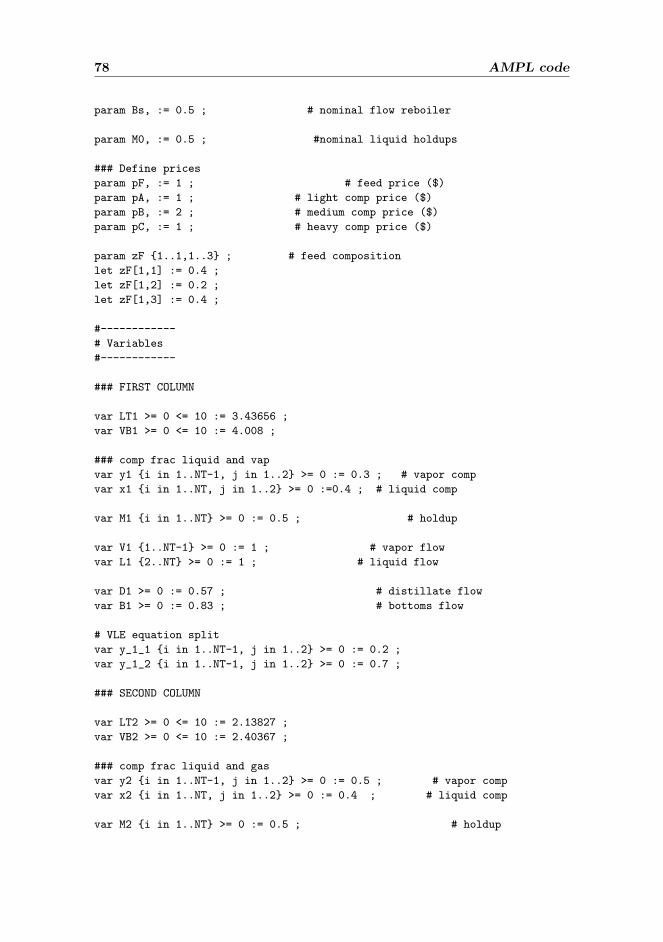
78 AMPL code

param Bs, := 0.5 ; # nominal flow reboiler

param M0, := 0.5 ; #nominal liquid holdups

### Define prices

param pF, := 1 ; # feed price ($)

param pA, := 1 ; # light comp price ($)

param pB, := 2 ; # medium comp price ($)

param pC, := 1 ; # heavy comp price ($)

param zF {1..1,1..3} ; # feed composition

let zF[1,1] := 0.4 ;

let zF[1,2] := 0.2 ;

let zF[1,3] := 0.4 ;

#------------

# Variables

#------------

### FIRST COLUMN

var LT1 >= 0 <= 10 := 3.43656 ;

var VB1 >= 0 <= 10 := 4.008 ;

### comp frac liquid and vap

var y1 {i in 1..NT-1, j in 1..2} >= 0 := 0.3 ; # vapor comp

var x1 {i in 1..NT, j in 1..2} >= 0 :=0.4 ; # liquid comp

var M1 {i in 1..NT} >= 0 := 0.5 ; # holdup

var V1 {1..NT-1} >= 0 := 1 ; # vapor flow

var L1 {2..NT} >= 0 := 1 ; # liquid flow

var D1 >= 0 := 0.57 ; # distillate flow

var B1 >= 0 := 0.83 ; # bottoms flow

# VLE equation split

var y_1_1 {i in 1..NT-1, j in 1..2} >= 0 := 0.2 ;

var y_1_2 {i in 1..NT-1, j in 1..2} >= 0 := 0.7 ;

### SECOND COLUMN

var LT2 >= 0 <= 10 := 2.13827 ;

var VB2 >= 0 <= 10 := 2.40367 ;

### comp frac liquid and gas

var y2 {i in 1..NT-1, j in 1..2} >= 0 := 0.5 ; # vapor comp

var x2 {i in 1..NT, j in 1..2} >= 0 := 0.4 ; # liquid comp

var M2 {i in 1..NT} >= 0 := 0.5 ; # holdup

79

var V2 {1..NT-1} >= 0 :=1; # vapor flow

var L2 {2..NT} >= 0 :=1; # liquid flow

var D2 >= 0 := 0.26 ; # distillate flow

var B2 >= 0 := 0.56 ; # bottoms flow

# VLE equation split

var y_2_1 {i in 1..NT-1, j in 1..2} := 0.3 ;

var y_2_2 {i in 1..NT-1, j in 1..2} := 0.8 ;

#----------------------------

# Model/Constraints 1

#----------------------------

### VLE equation split

const1 {i in 1..NT-1, j in 1..2} :

y_1_1[i,j] = x1[i,j]*m_alpha[j,j] ;

const2 {i in 1..NT-1, j in 1..2}:

y_1_2[i,j] = ((x1[i,1]*(alpha[1]-1)+x1[i,2]*(alpha[2]-1))+1) ;

### Vapour-liquid equilibria (multicomponent ideal VLE,

# Stichlmair-Fair, ’Distillation’, p. 36, 1998)

const3 {i in 1..NT-1, j in 1..2}:

y1[i,j] = y_1_1[i,j]/y_1_2[i,j] ;

### Vapor flows assuming constant molar flows


V1[i] = VB1 ; # vapor flow below feed


V1[i] = VB1 + (1-qF)*F ; # vapor flow above feed

### Liquid flows are given by Franci’s Weir Formula L(i)=K*Mow(i)^1.5

# Liquid flow L(i) dependent only on the holdup over the weir Mow(i)

#M(i)= Mow(i) + Muw(i) (Total holdup = holdup over weir +

#holdup below weir)

const6 {i in 2..NF}:

L1[i] = Kbf*(M1[i] - Muw)^1.5 ; # Liquid flow below feed


L1[i] = Kuf*(M1[i] - Muw)^1.5 ;# Liquid flows above feed

const8:

L1[NT] = LT1; # Condenser’s liquid flow

80 AMPL code

### Distillate and bottom

const9:

B1 = Bs + (M1[1] - MBs)*KcB ;

const10:

D1 = Ds + (M1[NT] - MDs)*KcD ;

### Material balances for total holdup and component holdup


L1[i+1] - L1[i] + V1[i-1] - V1[i] = 0 ; # dM below feed


L1[i+1] - L1[i] + V1[i-1] - V1[i] = 0 ; # dM above feed

const13 {i in 2..NF-1, j in 1..2}:

L1[i+1]*x1[i+1,j] - L1[i]*x1[i,j] + V1[i-1]*y1[i-1,j]

- V1[i]*y1[i,j] = 0 ;

const14 {i in NF+1..NT-1, j in 1..2}:


- V1[i]*y1[i,j] = 0 ;

### Correction for feed at the feed stage: The feed is assumed to

#be mixed into the feed stage

const15:

L1[NF+1] - L1[NF] + V1[NF-1] - V1[NF] + F = 0 ;

const16:

L1[NF+1]*x1[NF+1,1] - L1[NF]*x1[NF,1] + V1[NF-1]*y1[NF-1,1]

- V1[NF]*y1[NF,1] + F*zF[1,1] = 0 ;

const17:


- V1[NF]*y1[NF,2] + F*zF[1,2] = 0 ;

### Reboiler (assumed to be an equilibrium stage)

const18:

L1[2] - V1[1] - B1 = 0 ;

const19 {j in 1..2}:

L1[2]*x1[2,j] - V1[1]*y1[1,j] - B1*x1[1,j] = 0 ;

### Total condenser (no equilibrium stage)

const20:

V1[NT-1] - LT1 - D1 = 0 ;

const21 {j in 1..2}:

V1[NT-1]*y1[NT-1,j] - L1[NT]*x1[NT,j] - D1*x1[NT,j] = 0 ;

81

#----------------------------

# Model/Constraints 2

#----------------------------

### VLE equation split

const21 {i in 1..NT-1, j in 1..2} :

y_2_1[i,j] = x2[i,j]*m_alpha[j,j] ;

const22 {i in 1..NT-1, j in 1..2}:

y_2_2[i,j] = ((x2[i,1]*(alpha[1]-1)+x2[i,2]*(alpha[2]-1))+1) ;

### Vapour-liquid equilibria (multicomponent ideal VLE,

# Stichlmair-Fair, ’Distillation’, p. 36, 1998)

const23 {i in 1..NT-1, j in 1..2}:

y2[i,j] = y_2_1[i,j]/y_2_2[i,j] ;

### Vapor flows assuming constant molar flows


V2[i] = VB2 ; # vapor flow below feed


V2[i] = VB2 ; # vapor flow above

const26 {i in 2..NF}:

L2[i] = Kbf*(M2[i] - Muw)^1.5 ; # Liquid flow below feed


L2[i] = Kuf*(M2[i] - Muw)^1.5 ; # Liquid flow above feed

const28:

L2[NT] = LT2; # Condenser’s liquid flow

const29:

B2 = Bs + (M2[1] - MBs)*KcB ;

const30:

D2 = Ds + (M2[NT] - MDs)*KcD ;

### Material balances for total holdup and component holdup


L2[i+1] - L2[i] + V2[i-1] - V2[i] = 0 ; # dM below feed


L2[i+1] - L2[i] + V2[i-1] - V2[i] = 0 ; # dM above feed

82 AMPL code

const33 {i in 2..NF-1, j in 1..2}: # dMxdt below feed


- V2[i]*y2[i,j] = 0 ;

const34 {i in NF+1..NT-1, j in 1..2}: # dMxdt above feed


- V2[i]*y2[i,j] = 0 ;

### Correction for feed at the feed stage: The feed is assumed to be

# mixed into the feed stage

const35:

L2[NF+1] - L2[NF] + V2[NF-1] - V2[NF] + B1 = 0 ;

const36:

2[NF+1]*x2[NF+1,1] - L2[NF]*x2[NF,1] + V2[NF-1]*y2[NF-1,1]

- V2[NF]*y2[NF,1] + B1*x1[1,1] = 0 ;

const37:


- V2[NF]*y2[NF,2] + B1*x1[1,2] = 0 ;

### Reboiler (assumed to be an equilibrium stage)

const38:

L2[2] - V2[1] - B2 = 0 ;

const39 {i in 1..2}:

L2[2]*x2[2,i] - V2[1]*y2[1,i] - B2*x2[1,i] = 0 ;

### Total condenser (no equilibrium stage)

const40:

V2[NT-1] - LT2 - D2 = 0 ;

const41 {i in 1..2}:

V2[NT-1]*y2[NT-1,i] - L2[NT]*x2[NT,i] - D2*x2[NT,i] = 0 ;

### Inequality constraints

const42:

x1[NT,1] >= 0.95 ; # xA

const43:

x2[NT,2] == 0.95 ; # xB

const44:

1 - (x2[1,1]+x2[1,2]) >= 0.95 ; # xC

const45:

VB1 <= 4.008 ; # max boilup column 1

83

const46:

VB2 <= 2.405 ; # max boilup column 2

### Initial constraints for parameters

constF: F = nominal_F ;

constpV: pV = nominal_pV ;

# constzF: zF = nominal_zF ;

constqF: qF = nominal_qF ;

#--------------------

# OBJECTIVE FUNCTION

#--------------------

minimize cost: pF*F + pV*(VB1 + VB2) - pA*D1 - pB*D2 - pC*B2 ;

self-optimizing control structures for active constraint regions...

Documents