Self-enforcing Trade Agreements and Lobbying

Kristy Buzard

110 Eggers Hall, Economics Department, Syracuse University, Syracuse, NY 13244. 315-443-4079.

Abstract

In an environment where international trade agreements must be enforced via promises

of future cooperation, the presence of an import-competing lobby has important im-

plications for optimal punishments. When lobbies work to disrupt trade agreements, a

Nash reversion punishment scheme must balance two, conflicting objectives. Longer

punishments help to enforce cooperation by increasing the government’s costs of de-

fecting, but because the lobby prefers the punishment outcome, this also incentivizes

lobbying effort and with it political pressure to break the agreement. Thus the model

generates an optimal length for Nash-reversion punishments, and it depends directly on

the political influence of the lobbies. Trade agreement tariffs are shown to be increasing

in the political influence of the lobbies, as well as their patience levels.

Keywords:

trade agreements, lobbying, optimal punishments, repeated games, enforcement

1. Introduction

In the absence of strong external enforcement mechanisms for international trade

agreements, we generally assume that cooperation is enforced by promises of future

cooperation, or, equivalently, promises of future punishment for exploitative behavior.

When repeated-game incentives are used to enforce cooperation and prevent players

from defecting in a prisoner’s dilemma-style stage game, the strongest punishment is

Email address: kbuzard@syr.edu (Kristy Buzard)URL: http://faculty.maxwell.syr.edu/kbuzard (Kristy Buzard)Previously circulated under the title “Self-enforcing Trade Agreements, Dispute Settlement and Separa-

tion of Powers.”

Preprint submitted to Elsevier November 27, 2016

usually assumed to be the grim trigger strategy of defecting forever upon encountering

a defection by one’s partner.

I show that when lobbies are relevant players in the repeated game, the optimal

length of Nash-reversion punishments is often finite and can be derived directly from

the players’ incentive constraints. The logic behind these finite-length optimal punish-

ments is different from those currently in the literature, e.g. Green and Porter (1984) for

industrial organization or Park (2011) for trade agreements. To the best of my knowl-

edge, in all the environments that produce these results, the players spend some time

in the punishment phase, usually due to imperfect monitoring and/or uncertainty. Thus

the shortening of the punishment serves to increase welfare by minimizing time spent

in punishment periods. The results of this paper are of a different nature, as the players

remain in the cooperative state in all periods. Here, the gain comes from loosening a

player’s incentive constraint so that cooperative state welfare is higher.

Not only does adding lobbies suggest an optimal length for punishments that fea-

ture periods of Nash-reversion-style non-cooperation; it also turns out that this optimal

punishment length itself depends on how readily special interests are able to influence

the political process. That is, the optimal length of punishments is a function of the

strength of the lobbies, reinforcing the idea that including lobbying in such analyses

can be can be critically important for institutional design questions. We shall also see

that, for a fixed punishment length, as lobbies become more influential or more patient,

the equilibrium trade agreement tariff that must be provided in order to overcome the

ratification hurdle increases.

The structure of the model is similar to that of Bagwell and Staiger (2005) with

two main changes: the political-economy weights are endogenously determined and in

place of a unitary government that has different preferences before and after signing a

trade agreement, this model has two branches of government with differing preferences

who share policy-making power as in Milner and Rosendorff (1997), Song (2008) and

Buzard (2016). The model does admit an interpretation in which the same branch

of government both negotiates the trade agreement and decides on the applied tariff

ex-post. In this sense, the structure of the one-shot game shares much in common

with Maggi and Rodrıguez-Clare (2007). Sections 3.1 and 4 discuss the connections

2

between this model and Maggi and Rodrıguez-Clare (2007).

This paper is the first to incorporate endogenous lobbying along the lines of Gross-

man and Helpman (1994, 1995) into a repeated-game setting. Here, welfare-maximizing

executives use their control over trade-agreement tariffs as a kind of political commit-

ment device:2 by setting tariffs to optimally reduce lobbying incentives, the executives

reduce the political pressure on the legislatures. This changes the legislatures’ incen-

tives so that they do not break the agreement as they would have if they had faced more

intense political pressure.3

Given that all actors have perfect information about the effect of lobbying effort on

the outcome of the political process, the executives maximize social welfare by choos-

ing the lowest tariffs that make it unattractive for the lobbies to provoke the legislature

to initiate a trade dispute.4 So even though there are no disputes in equilibrium, the out-

of-equilibrium threat that a lobby might provoke a trade war is crucial in determining

the equilibrium trade agreement structure.

Thus the problem with the lobby has an extra constraint relative to the standard

problem. The constraint on the key repeated-game player, which I refer to as the leg-

islature, is loosened by increasing the punishment length because defections become

relatively more unattractive. However, the new constraint due to the presence of lobby-

ing becomes tighter as the punishment becomes more severe because the lobby prefers

punishment periods. Because the tariffs during punishment, and thus the lobby’s prof-

its, are higher than the tariffs during a cooperative period, the lobby has increased

2This is a different kind of domestic commitment role for trade agreements than that identified by Maggiand Rodrıguez-Clare (2007), who show that trade agreements can be useful for helping governments commitvis-a-vis private firms in their investment decisions.

3This is not to say that the legislature itself is made better off by the reduction in political pressure,although Buzard (2015) demonstrates that this is possible. It only means that the executive can use thecommitment power of the trade agreement to improve its welfare, which is assumed to differ from that ofthe legislature. The commonly-made assumption that the executive is less protectionist than the legislatureis a special case of the finding that susceptibility to special interests generally declines with the size of one’sconstituency. One simple illustration from the realm of trade policy is the following: a legislator whosedistrict has a large concentration of a particular industry does not take into account the impact of tariffson the welfare of consumers in other districts, while the executive, whose constituency encompasses thewhole country, will internalize these diffuse consumption effects. For a detailed argument, see Lohmann andO’Halloran (1994).

4With no uncertainty of any kind, there will be no trade disputes in equilibrium. Political uncertaintycan be easily added to the model, in which case lobbying effort is typically non-zero and there is a positiveprobability of dispute in equilibrium.

3

incentive to exert effort as the punishment lengthens.

The optimal punishment length must balance these two competing forces. Where

the balance falls depends in large part on how influential the lobby is in the legislative

process. If the lobby has very little power, the optimal punishment converges to that of

the model without a lobby: longer punishments are better because the key constraint

is the legislature’s. As the lobby becomes stronger, the optimal punishment becomes

shorter because the lobby’s incentive becomes more important.

Quite intuitively, it is also shown that, for a given punishment length, increases

in the lobby’s strength lead to lower required payments to provoke trade dispute and

therefore higher equilibrium trade agreement tariffs to avoid those disputes. Increases

in the lobby’s patience have the same qualitative effects, while increases in the patience

of the legislature work in the opposite direction: the lobby must pay more to induce the

legislature to endure the punishment and the executive can accordingly reduce trade

agreement tariffs without fear that the agreement will be broken.

Repeated non-cooperative game models of trade agreements have been considered

by McMillan (1986, 1989), Cotter and Mitchell (1997), Dixit (1987), Bagwell and

Staiger (1990, 1997a,b, 2002), Kovenock and Thursby (1992), Maggi (1999), Edering-

ton (2001), Ludema (2001), Rosendorff (2005), Klimenko, Ramey and Watson (2008),

Bagwell (2009), and Park (2011).

In particular, Hungerford (1991), Riezman (1991), Cotter and Mitchell (1997),

Bagwell (2008) and Martin and Vergote (2008) consider the impact of different as-

sumptions about reactions and timing of punishments for deviations from agreements.

Here, I study a very simple structure in which the two trading partners remain in a

symmetric trade war for a predetermined number of periods.

The model would require modification in order to match a multilateral agreement

with many goods, for instance specifying that trade goes on as usual in all those in-

dustries except the one in which the applied tariff is raised above the tariff cap and

the industry the trading partner chooses to use for retaliation. But the basic intuition

goes through: the incentives of lobbies should be taken into account when designing

punishment schemes because the length of time a lobby can expect to enjoy a higher

trade-war tariff is directly related to whether the lobby finds it worthwhile to exert effort

4

in provoking a punishment phase in the first place.5

In line with this fundamental idea, I discuss an alternative punishment scheme that

involves the defecting party applying a zero tariff during the punishment phase. This

can support lower trade agreement tariffs than reverting to the stage-game subgame-

perfect Nash equilibrium because these low tariffs significantly weaken the lobby’s

incentive to exert effort to break the trade agreement. I am not aware of such punish-

ments being applied in actual trade agreements, and this may be because other consid-

erations rule out this type of punishment. But it is worth considering whether some

such alternative punishment structure that takes into account lobbying incentives may

be implementable and thus capable of supporting greater levels of cooperation.

The model under consideration here can only speak directly to motives for pure

rent-seeking and not to responses to unpredictable changes in the economic and polit-

ical environment since such uncertainty is assumed away. This means that measures

designed to provide escape are not beneficial in this environment (cfr. Bagwell and

Staiger (2005), Buzard (2015)). With no uncertainty, disputes should not be observed

on the equilibrium path. In reality, of course, there is considerable such uncertainty,

but it’s not clear that this is the sole source of the trade disputes that arise.

For instance, the immediate retaliation that ensures self-enforcement in this model

is rarely possible under current trading rules and this may well increase the number

of disputes observed in equilibrium. One possibility for implementing more immedi-

ate retaliation is the idea proposed in the literature that trading partners exact ‘vigilante

justice’ through various means such as imposing unrelated anti-dumping duties.6 How-

ever, this would not necessarily reduce the number of disputes if the original defector

objects to the new anti-dumping measure. In order for the ‘vigilante justice’ option to

work as a punishment in the context of this model, the original defector would have to

tacitly acknowledge it as punishment and play along.

5The model can also be applied to Preferential Trade Agreements with some additional modifications dueto the restrictions imposed by GATT Article XXIV. Since the interpretation of the restriction that PTAs cover‘substantially all the trade’ has never been settled in law, there remains significant scope to grant non-zerotariffs to industries who exert sufficient lobbying effort.

6See the discussions in Bown (2005) and Martin and Vergote (2008) for evidence on informal versusformal retaliation.

5

I begin in the next section by describing in detail the model, which is closely re-

lated to the model in Buzard (2016). Both papers employ the separation-of-powers

government structure with endogenous lobbying. While the current paper focuses on

the implications of self-enforcement constraints for the optimal design of trade agree-

ments, Buzard (2016) abstracts from enforcement issues and demonstrates that taking

into account the separation-of-powers structure can shed light on the empirical puzzle

surrounding the Grossman and Helpman (1994) ‘Protection for Sale’ model, highlights

the importance of the threat of ratification failures on the formation of trade agreements

and examines the role of political uncertainty in the policy-making process.

Section 3 explains the way in which the trade agreement negotiation process selects

a particular class of equilibria and describes that class of equilibria. I characterize the

structure of trade agreements in this environment in Section 4 and their properties in

Section 5. I explore the punishment-length decision in Section 6. Section 7 demon-

strates these results via a parameterized model and Section 8 explores an alternative

punishment scheme. Section 9 concludes. AppendixB analyses unitary models in line

with Maggi and Rodrıguez-Clare (2007) and Dixit, Grossman and Helpman (1997) as

well as a comparison of the main model with tariff caps to one with strong bindings.

2. The Model

This is a model of repeated interaction where the executive branches of each of

two countries jointly restrict the repeated interaction of the other players by choosing

the trade agreement tariff in period zero. In every period thereafter the legislatures

and lobbies interact in a stage game to determine lobbying effort and the applied tariff

levels that impact the economic outcomes for consumers and producers in the two-

country economy.

The stage game of the repeated game is slightly more complex than in a standard

repeated-game model of trade agreements in that each period of the repeated game has

two phases. In the first phase, each lobby decides how much effort to exert to influence

its respective legislature’s tariff setting. In the second phase, the legislatures then set

the applied tariff levels.

6

Section 2.1 describes consumers’ preferences as well as the technologies of pro-

duction and trade. Section 2.2 details the stage game interaction between the lobby and

legislature within each country, while Section 2.3 outlines the structure governing the

players’ repeated interaction.

2.1. The Basic Setup

This section details the two-country, two-good partial equilibrium model that is em-

ployed throughout the paper. Home country variables appear with no asterisk, while

foreign country variables are differentiated with the addition of an asterisk. The coun-

tries trade two goods, X and Y , where Pi denotes the home price of good i ∈ X,Y and P ∗

i denotes the foreign price of good i. The demand functions are taken to be iden-

tical in each country for both traded goods, respectively D(Pi) in home and D(P ∗

i ) in

foreign and are assumed strictly decreasing and twice continuously differentiable.

The supply functions for good X are QX(PX) and Q∗

X(P ∗

X) and are assumed

strictly increasing and twice continuously differentiable for all prices that elicit positive

supply. I assume Q∗

X(PX) > QX(PX) for any such PX so that the home country is a

net importer of good X . The production structure for good Y is taken to be symmetric,

with demand and supply such that the economy is separable in goods X and Y .

As is standard, I assume that the production of each good requires the possession of

a sector-specific factor that is available in inelastic supply, is non-tradable, and cannot

move between sectors so that the income of owners of the specific factors is tied to the

price of the good in whose production their factor is used. In order to focus attention

on protectionist political forces, I assume that only the import-competing industry in

each country is politically-organized and able to lobby and that it is represented by a

single lobbying organization.7

For simplicity, I assume each government’s only trade policy instrument is a spe-

cific tariff on its import-competing good: the home country levies a tariff τ on good

X while the foreign country applies a tariff τ∗ to good Y . Local prices are then

PX = PWX + τ , P ∗

X = PWX , PY = PWY and P ∗

Y = PWY + τ∗ where a W superscript

7Adding a pro-trade lobby for the exporting industry would modify the magnitude of the effects and makefree trade attainable for a range of parameter values, but it would not modify the essential dynamic.

7

indicates world prices.

The following market clearing conditions determine equilibrium prices:

MX(PX) =D(PX) −QX(PX) = Q∗

X(P ∗

X) −D(P ∗

X) = E∗

X(P ∗

X)

EY (PY ) = QY (PY ) −D(PY ) =D(P ∗

Y ) −Q∗

Y (PY ) =M∗

Y (P ∗

Y )

where MX are home-county imports and E∗

X are foreign exports of good X and EY

are home-county exports and M∗

Y are foreign imports of good Y .

It follows that PWX and PWY are decreasing in τ and τ∗ respectively, while PX and

P ∗

Y are increasing in the respective domestic tariff. This leads to a standard terms-of-

trade externality. As profits and producer surplus—identical in this model—in a sector

are increasing in the price of its good, profits in the import-competing sector are also

increasing in the domestic tariff. This economic fact combined with the assumptions

on specific factor ownership is what motivates political activity.

Payoffs in the strategic model will be given in terms of the profits, consumer sur-

plus, and imports (i.e. tariff revenue) calculated from these fundamentals, all as func-

tions of tariffs, or equivalently, prices.

2.2. The Stage Game

As the economy is fully separable and the economic and political structures are

symmetric, I focus on the home country and the X-sector. The details are analogous

for Y and foreign.

The home lobby’s payoff within a period is

UL = πX(τ) − e (1)

where πX(⋅) is the current-period profit of the import-competing industry and τ is

the home country’s tariff on the import good. I assume the lobby’s contribution is

observable to its own legislature but is not observable to the foreign legislature.8 I

represent a vector of tariffs for both countries (τ, τ∗) as a single bold τ .

8The implication of this assumption is that the lobby can directly influence only the home legislature,and so the influence of one country’s lobby on the other country’s legislature occurs only through the tariffsselected. See for reference Grossman and Helpman (1995), page 685-686.

8

The per-period welfare function of the home legislature, whose decisions I model

as being taken by a median legislator, is

WML = CSX(τ) + γ(e) ⋅ πX(τ) +CSY (τ∗) + πY (τ∗) +TR(τ) (2)

where CS is consumer surplus, π are profits and TR is tariff revenue. Here, the weight

the median legislator places on the profits of the import-competing industry, γ(e), is af-

fected by the level of lobbying effort. That is, the level of lobbying effort identifies the

median legislator and therefore the median legislator’s political-economy weight. No-

tice that a key element of the ‘preferences’ of the legislature, which represent the pro-

cess by which a decision is made, are embodied in the function γ(⋅) and this does not

change with time or the institutional environment. Only the outcome of the decision-

making process changes with e, that is, which legislator holds the decisive vote.

Aside from the endogeneity of the weight the legislature places on the lobbying

industry’s profits, this is precisely the deus ex machina government objective function

popularized by Baldwin (1987) that is commonly employed in the literature on the

political economy of trade agreements. Since trade policies are often determined within

the context of trade agreements, it is useful to have a framework to bring together the

endogenous political pressure of ‘Protection-for-Sale’-style modeling with the trade

agreements approach; the formulation in Equation 2 is intended to be a bridge between

the two.

In the literature that studies the design of trade agreements and institutions, political

pressure is taken to exogenously impact the value politicians place on producer surplus.

Here, that level of political pressure is taken to be determined by lobbying effort, which

can be interpreted broadly as any action that serves to increase the weight that the

median legislator places on producer surplus when taking decisions. Modeling the

objective function so closely on the standard in the trade agreements literature allows

for direct comparisons to the large extant body of work that studies exogenous shocks.

Assumption 1. γ(e) is continuously differentiable, strictly increasing and concave ine.

Assumption 1 formalizes the intuition that the legislature favors the import-competing

industry more the higher is its lobbying effort, but that there are diminishing returns

9

to lobbying activity.9 The assumption of diminishing returns to lobbying effort has

been present in the literature going back at least to Findlay and Wellisz (1982). Dixit,

Grossman and Helpman (1997) point out the linearity in contributions assumed in the

Protection for Sale model prevents complete analysis of distributional questions and

restricts the returns to lobbying activity to be constant.

The functional form in Expression 2 with Assumption 1 can be interpreted as a

special case of the general welfare function proposed in Dixit, Grossman and Helpman

(1997) in which the median legislator’s welfare exhibits decreasing returns to lobbying

effort.10 The interpretation is that the identity of the median legislator changes ever

more slowly as lobbying effort increases because it becomes more difficult for the

lobby to win additional votes given that the most friendly legislators are targeted first.

In AppendixB.2, I demonstrate that an appropriately-stylized version of the Dixit,

Grossman and Helpman (1997) model produces results that that are, in fact, qualita-

tively similar to those of the model presented here. It is also easy to show that the

results of the model are unchanged if the lobby’s effort is subtracted from the ex-

ecutive’s and/or the median legislator’s welfare function, a consideration that seems

more important to take into account in this context of non-transferable utility. I do

not subtract lobbying effort from the government welfare functions in order to main-

tain consistency with the literature (e.g. Grossman and Helpman (1994) and Maggi

and Rodrıguez-Clare (2007) where utility is transferable between the government and

lobby and Dixit, Grossman and Helpman (1997) and Limao and Tovar (2011) where it

is not).

2.3. The Repeated Game

This trade policy environment has many features of a standard prisoner’s dilemma.

Most importantly, the legislatures face unilateral incentives to violate the terms of any

trade agreement under pressure from the lobbies. When the legislatures and lobbies set

tariffs at a higher, non-cooperative or “trade war” level, payoffs for the social-welfare

9The diminishing returns here take the form of declining increments to the lobby’s influence as effortincreases; in Ethier (2012), the returns to lobbying decline with higher levels of protection.

10Note that while Dixit, Grossman and Helpman (1997)’s model nests both the model presented in thispaper and that of Grossman and Helpman (1994), neither of the latter two are generalizations of the other.

10

conscious executives are reduced. In order to maintain the trade agreement without

external enforcement, we turn to incentives within the context of an infinitely-repeated

game.

The timing of the game is as follows. At time zero, the executives set trade policy

cooperatively in an international agreement. Time zero will be addressed in detail in

Section 3.1. The stage game is then repeated in each period t ∈ 1,2, . . ..

Because this repeated game has a dynamic structure as described in Section 2.2, it

is important to carefully describe the informational set-up. Although the assumption

from the stage game that lobbying activity is not observable across international borders

extends to the repeated game, that is, there is no learning across periods about lobbying

effort, the tariff levels are perfectly observable across borders and across time, as well

as within the stage game.

The players’ payoffs are discounted according to the discount factors δML for the

median legislator, δL for the lobby and δE for the executive branch.

3. Equilibrium Selection and Analysis

I examine a particularly simple and realistic class of equilibria that have the follow-

ing features.

First, these are public perfect equilibria (PPE) in a particular sense that is appro-

priate for the multi-phase stage-game. Given the game’s structure and the assumption

that lobbying effort is not observable across international borders, players in the same

country can take advantage of more information than those who are in different coun-

tries. In equilibrium, I assume that this extra information is only used within a period

so that players’ behavior within a period is conditioned on the behavior in previous pe-

riods only through the history of the publicly-observable tariff levels that were chosen.

That is, the solution concept employed here is perfect public equilibrium (PPE) period

to period. Whenever there is a possibility of multiple equilibria, I focus on the one that

maximizes the welfare of the executives.

Second, I focus on those equilibria that are best in terms of the executives’ welfare

given a simple punishment scheme. For all results except those in Section 8, deviations

from the trade agreement are punished by reverting to the stage game subgame-perfect

11

Nash equilibrium for a specified number of periods before returning to cooperation.

For convenience, I will refer to these punishments as ‘limited Nash reversion’ punish-

ments or ‘T-period Nash reversion’ punishments. Section 3.4 states the full equilibrium

strategy profiles and establishes that they constitute an equilibrium.

These limited Nash reversion punishments represent a trade war that is limited in

duration and therefore more realistic than infinite Nash reversion. In the environment

assumed here, any equilibrium in this class will have the feature that the trade agree-

ment tariff will be set at the same level for all periods.

We can think of the limited Nash reversion punishment scheme, including the num-

ber of periods of punishment T , as being chosen by the executives, a supranational

body like the WTO, or some combination of the two. In Section 6, the question of how

to optimally design the punishment scheme within the class of T -period Nash rever-

sion punishments is addressed. Until then, I take the punishment length T to be given

exogenously.

After exploring the role of the executives in shaping the trade agreement in Sec-

tion 3.1, I detail the non-cooperative stage-game equilibrium in Section 3.2. Section 3.3

explores the repeated-game incentives that are necessary to sustain cooperation. Sec-

tion 3.4 then establishes the repeated game equilibrium.

3.1. Time Zero: Trade Agreement Negotiation

Given the punishment length T , the executives determine the specific equilibrium

by choosing the trade agreement tariffs—which I assume take the form of tariff caps—

to maximize joint social welfare. They have no other opportunity to affect the outcome

of the trading relationship. Because the executives face the constraint that the trade

agreement tariff caps they choose must be consistent with equilibrium play by the leg-

islatures and lobbies, one can view their choice of the trade agreement tariffs as setting

a key parameter for the repeated game.

I model the choice of the trade agreement tariff parameter in the following way. I

assume that the negotiating process by which the executives choose the trade agreement

tariffs τa = (τa, τ∗a) is efficient given their welfare functions WE(τa) (home) and

12

W ∗

E (τa) (foreign).11. In this symmetric environment, this process maximizes the joint

payoffs of the trade agreement12

WE(τa) =WE(τa) +W ∗

E (τa) (3)

subject to the constraints that the legislatures and lobbies won’t behave in a way that

violates the agreement and that they also behave rationally during any punishment

sequence. I will say more about these constraints in the following subsections.

I model the executives’ choice via the Nash bargaining solution. The disagree-

ment point is the executives’ welfare resulting from the Nash equilibrium in the non-

cooperative game (i.e. in the absence of a trade agreement) between the legislatures.

The executives are assumed to be social-welfare maximizers who can make trans-

fers between them.13 Therefore the home executive’s welfare is specified as follows:

WE = CSX(τ) + πX(τ) +CSY (τ∗) + πY (τ∗) +TR(τ) (4)

Note that this is identical to the welfare function for the legislature aside from the

weight on the profits of the import industry, which is not a function of lobbying effort

and here is assumed to be 1 for simplicity.

The idea is that lobbying has less of an impact during trade agreement negotiations—

embodied in the executive’s objective function—than it does during day-to-day trade

policy making, which is embodied in the legislature’s objective function. This set-up

represents the difference between the impact of lobbying during the two phases in a

simple, albeit extreme, way that permits a focus on the out-of-equilibrium threat of

trade disruption created by the lobbies.14

This stylized modeling of objective functions can accommodate real-world insti-

tutions such as those in the United States where the Congress has some consultative

11The executives’ welfare functions are specified in detail in Equation 4 below.12If political uncertainty is present, the joint payoffs must take into account the possibility that the trade

agreement will be broken. In the case of certainty, agreement will always be maintained on the equilibriumpath and so this specification is sufficient.

13It is trivial to relax the assumption of social-welfare maximizing executives; in the present symmetricenvironment with no disputes, the same is true of the assumption about transfers.

14The model can accommodate lobbying at the trade-agreement formation phase. This adds an interestingquestion of how lobbies make a resource allocation decision between the two phases. This is left for futurework.

13

role in trade agreement negotiations and the executive branch has the ability to alter

applied tariffs under important administrative procedures such as anti-dumping and

safeguard measures.15 Consider the following, alternative interpretation of the model.

Assume there is only one decision-making body but the lobby is not active during the

ex-ante phase, that is, when the trade agreement is being negotiated. For ease of ex-

position, take this single decision-making body to be the legislature so that the single

decision-making body has the preferences in Expression 2. At the ex-ante stage, the

welfare function would reduce to that in Expression 4. This interpretation fits into the

framework of Maggi and Rodrıguez-Clare (2007) by assuming that capital is perfectly

mobile in the long run so that it is not worthwhile for the lobby to expend resources to

influence the negotiation of the trade agreement.16 Note that this remains a non-unitary

model. Out of a single decision-making body, the level of lobbying effort determines a

different decisive member depending on the situation, e.g. during ex-ante negotiations

(e = 0) versus a trade war (e = etw). A unitary model—in which a single actor makes

different decisions depending on how much lobbying effort she experiences—results

in minor, qualitative changes to the results. I discuss the unitary version of the model

in AppendixB.1. Note that in either case, it is only the realization of γ(⋅) that changes

with e, not the preferences themselves which are embodied in γ(⋅).

Note that one does not have to make this stark assumption that there is no lobbying

during the trade agreement phase. What is required is that the government’s preferences

during this phase are not directly altered in a significant way by lobbying over trade.

For trade policy, where there are concentrated benefits but harm is diffuse, there are

good reasons for the legislature to be more protectionist than the president, as has

been the case in the post-war United States. Because the President has the largest

15It is, however, debatable whether many of these procedures fall under the scope of the issues consideredin this paper since they are often WTO-legal and therefore do not serve to violate the trade agreement. Inany case, the conditions under which these procedures would be necessary in a trade agreement—wheresubsidies are a policy choice (countervailing duties), there is uncertainty about the trading environment(escape clause) or markets are not perfectly competitive (anti-dumping)—are not present in the environmentunder consideration here.

16To match the assumption of a social-wefare maximing executive, this requires the additional assumptionthat γ(0) = 1. The model is qualitatively unchanged for other values of γ(0) as long as the analogue ofAssumption 2 below holds.

14

constituency possible, delegating authority to the executive branch may simply be a

mechanism for “concentrating” the benefits since consumers seem unable to overcome

the free-riding problem. In fact, a strong argument can be made that power over trade

policy has been delegated to the executive branch precisely because it is less susceptible

to the influence of special interests (Destler 2005).

Therefore, in line with both the theoretical and empirical literature, I assume the

executive is at least weakly less protectionist than the legislature for all outcomes of

the lobbying process.

Assumption 2. γ(e) ≥ 1 ∀e.

Assumption 2 ensures that the trade agreement tariff is less than the tariff that re-

sults from unconstrained interaction between the lobby and legislature, which I denote

τ tw and explain in Section 3.2. More generally, it guarantees that the legislature’s in-

centives are more closely aligned with the lobby’s than are those of the executive. This

is not essential but simplifies the analysis and matches well the empirical findings that

politicians with larger constituencies are less sensitive to special interests (See Destler

(2005) and footnote 3 above).

Although the political process here matches most closely that of the United States

in the post-war era, I believe the model or one of its extensions is applicable for a

broad range of countries for which authority over the formation and maintenance of

trade policy is diffuse and subject to political pressure either at home or in a trading

partner.17

3.2. Stage Game Subgame Perfect Nash Equilibrium

Given the tariff caps that are chosen by the executives, any deviation from the trade

agreement will incur a limited Nash reversion punishment. Here I detail the stage-game

subgame-perfect Nash equilibrium strategies that are played during each period of such

a reversion. The legislature’s strategy is to choose the tariff that unilaterally maximizes

Equation 2 given τ∗ and the lobby’s effort level e. The separability of the economy

17In particular, the binary decision by the legislature about whether to abide by or break the trade agree-ment is modeled on the “Fast Track Authority” that the U.S. Congress granted to the Executive branch almostcontinuously from 1974-1994 and then again as “Trade Promotion Authority” from 2002-2007.

15

implies that there are no cross-country interactions in the decision problems, so the

home and foreign best response tariffs are independent and the home country’s tariff in

a punishment period maximizes weighted home-country welfare in the X-sector only.

The foreign legislature’s decision problem is analogous, and unilateral optimization

leads to what I refer to as τR as the solution to the following first order condition:18

∂CSX(τ)∂τR

+ γ(e) ⋅ ∂πX(τ)∂τR

+ ∂TR(τ)∂τR

= 0 (5)

The lobby chooses its effort e given the above best response tariff-setting behavior

by maximizing its profits net of effort: πX (τR (γ (e))) − e. This implies a first order

condition ofdπX(τR(γ(e)))

de= 1 (6)

That is, during this phase, the lobby chooses the level of effort that equates its expected

marginal increase in profits with its marginal payment. I label this effort level etw

because the result of unilateral optimization within the stage-game is taken to be the

trade war outcome. Similarly, I label τR(γ(etw)) as τ tw, the trade war tariff.19

3.3. Conditions for Cooperation

Here I focus on the key issue of the conditions under which the legislature decides,

for a given punishment length T and trade agreement tariffs τa, to adhere to the trade

agreement instead of violating it and triggering a punishment sequence. A central

insight is that we must directly take account of the lobby’s incentives when deriving the

condition under which the legislature adheres to the trade agreement. This is necessary

because the lobby’s effort choice plays a key role in determining whether or not the

legislature will break the trade agreement.

18That the second order condition is satisfied is not guaranteed. See the appendix of the working paperversion of Buzard (2016) for a discussion as well as a sufficient condition when prices are linear in tariffs.At issue is the need to bound the impact of the convexity of the profit term relative to the concavity of theconsumer surplus term for any given value of γ.

19The most general condition that ensures that the lobby’s second order condition holds is the following:

∣ ∂τ∂γ

∂2γ∂e2

∣ > ∂πX∂τ

[ ∂γ∂e

]2

∂2πX∂τ2

[ML’s SOC]2. Note that to ensure concavity of the lobby’s objective function, it’s

important that the decreasing returns to lobbying effort outweigh the direct impact of effort in increasingthe weighting function. Also, if profits either increase too fast in tariffs or are too convex, the second ordercondition can be violated.

16

Recall that the trade agreement is broken when the median legislator chooses a tariff

that is higher than the trade agreement level, τa. A tariff level that would violate the

trade agreement is chosen in the same manner as the trade war tariff, that is, according

to Equation 5. The legislature will, however, only choose to break the trade agreement

if the discounted stream of payoffs it receives from breaking the agreement is higher

than the discounted stream of payoffs it receives from abiding by the agreement. The

incentive constraint for the median legislator is a condition on the trade agreement

tariffs τa for a given T . It can be written as

WML(γ(eb),τa) + δMLVA

ML ≥WML(γ(eb), τR(eb), τ∗a) + δMLVP

ML

where V AML is the median legislator’s continuation value from the period after the break

decision when it abides by the trade agreement; V PML is the analogous continuation

value when it defects and is punished. I denote lobbying effort during a period in

which the legislature could break the trade agreement as eb.

If the Nash reversion punishment lasts for T periods, then the only part of the

discounted payoff stream we need to consider is the current period and the following T

periods: after those T periods, the trade agreement will be in force so the continuation

value from period T + 1 on will be the same whether or not the agreement is broken.

Therefore we have20

WML(γ(eb),τa) +δML − δT+1

ML

1 − δMLWML(γ(eb),τa) ≥

WML(γ(eb), τR(eb), τ∗a) +δML − δT+1

ML

1 − δMLWML(γ(eb),τ tw). (7)

Note that the median legislator, whose identity is determined by the lobby’s effort level

eb, evaluates future payoffs according to her own political economy weight, γ(eb).

Depending on legislator eb’s choice, either legislator ea or legislator etw will be the

decision maker in those future periods. But legislator eb, who is the decision maker in

the current period, maximizes her own welfare given the predicted behavior of future

decision makers.21

20Note that δ + δ2 + . . . + δl = ∑lk=1 δk = ∑∞k=1 δk −∑∞k=l+1 δk =δ

1−δ− δ

l+1

1−δ= δ−δl+1

1−δ.

21See Appendix AppendixB.1 for a version of the model with a unitary legislature. The results of thatmodel are broadly similar to the results of this non-unitary model.

17

Built into Condition 7 is the legislature’s applied tariff-setting behavior when eb is

below the cutoff value e(τa) that leads the legislature to break the trade agreement.22

Label the effort level at which the legislature chooses a particular τa as its optimal uni-

lateral tariff as ea(τa). For any eb weakly between ea(τa) and e(τa), the legislature

chooses τa as the applied tariff. If eb < ea(τa), the legislature chooses the correspond-

ing applied tariff, which is necessarily less than τa. Because the lobby’s net profits

are highest at τ tw, when the lobby does not choose e(τa), it will necessarily choose

ea(τa) and the applied tariff will be τa.

The condition for the lobby is given in Expression 8. Under the trade agreement,

a break in the trade agreement, and punishment period, the lobby receives its profits at

the chosen tariff level net of the effort level it exerts:

πX(τa) − ea(τa) +δL − δT+1

L

1 − δL[πX(τa) − ea(τa)] ≥

πX(τR(eb)) − eb +δL − δT+1

L

1 − δL[πX(τ tw) − etw] . (8)

The trade agreement tariffs are thus chosen by the executives according to the fol-

lowing joint maximization problem:

maxτa

WE(τa)1 − δE

subject to (9)

δML − δT+1ML

1 − δML[WML(γ(eb),τa) −WML(γ(eb),τ tw)] ≥

WML(γ(eb), τR(eb), τ∗a) −WML(γ(eb),τa) (10)

and

eb ≥ πX(τR(eb))−πX(τa)+ea(τa)+δL − δT+1

L

1 − δL[πX(τ tw) − etw − πX(τa) + ea(τa)]

(11)

where Inequalities 10 and 11 are simple rearrangements of 7 and 8.

Section 4 explores the structure of the equilibrium trade agreement given this prob-

lem faced by the executives.

22The determination of e(τa) is described in the next section.

18

3.4. Summary of Equilibrium Conditions

I now turn to a full description of the strategies and incentives for the equilibrium

that is selected by the executives’ choices as detailed in Section 3.1. Again, this is

a symmetric equilibrium, so I describe strategies for the home country only; similar

conditions hold for the foreign country.

Note again that, although the stage game has two phases and the players within a

country may use non-public information within a stage game, the equilibrium is in pub-

lic perfect strategies so players condition their behavior only on the publicly-observable

history of tariffs across periods.

At time t = 1, in any period following a period when the trade agreement has

been adhered to, or after the successful completion of a punishment, the lobby chooses

eb = ea(τa) and the legislature chooses τa, that is, to abide by the agreement by

implementing the tariff cap.

Any period t in which a violation of the agreement occurred j + 1 periods previous

for j ∈ [0, T − 1] with limited Nash reversion punishments initiated j < T periods

previous and followed in every period until t will be labeled a punishment period. In

a punishment period, the lobby chooses e ≥ etw and the legislature chooses a tariff at

least as large as its unilateral best response given e. Players ignore any deviations from

punishment-period prescribed play.23

Having fully described the strategies accompanying this punishment scheme, it

must be shown that they constitute a public perfect equilibrium, i.e. the strategies

constitute a subgame perfect Nash equilibrium from the start of each date and for each

public history as well as within each period.

Section 3.3 establishes that the cooperative-phase behavior is incentive compatible

for both the lobby and legislature given the limited Nash-reversion punishments. Thus

here we must show that it is incentive compatible to play the limited Nash-reversion

punishments given the rest of the scheme.

Section 3.2 shows that both the lobby and legislature are playing stage-game best

23T -period Nash reversion punishments are not necessarily public perfect since the players may want toinfluence the future path of play during punishment periods. Public perfection can be ensured by specifyingthat all players ignore any deviations from the punishment by any other player.

19

responses during any period of the punishment. Thus there is no deviation that creates

a stage-game improvement for either the lobby or the legislature given the stage-game

subgame-perfect Nash equilibrium strategies. Since all players’ strategies specify that

deviations are ignored, the continuation payoff from period t + 1 also cannot be im-

proved upon because it does not depend on the actions that are chosen at time t. Thus

play during a punishment sequence is not conditioned on what happens from period to

period and there is no profitable deviation from the prescribed strategy for any actor in

any period of the punishment.

As for the incentives of the actors in foreign country, recall that they cannot ob-

serve the level of lobbying expenditure, so they cannot react to deviations by the lobby.

Although they could in principle respond to deviations by the legislature, all other

players are ignoring deviations. Given this fact and the symmetry of the game, the

immediately-preceding argument concerning deviations from the punishments by the

home lobby and legislature can be applied to the lobby and legislature in the foreign

country.

Thus the posited equilibrium supported by T-length reversions to the stage-game

subgame-perfect Nash equilibrium is public perfect from period to period.

4. Trade Agreement Structure

To understand how the executives optimally structure trade agreements subject to

the given T -period Nash reversion punishment scheme, we must first examine the in-

centives of the lobbies and how the legislatures make decisions regarding breach of the

trade agreement. The model’s symmetric structure permits us to restrict attention to the

home country.

I consider the economically interesting case in which, for a given T and δ =(δE, δML, δL), the lowest supportable cooperative tariffs are strictly lower than the trade-

war (i.e. non-cooperative) level. If there is no non-trivial trade agreement in the ab-

sence of lobbying, the lobby has no incentive to exert effort to break the trade agree-

ment and the extra constraint implied by the presence of the lobby does not bind.

When deciding whether to exert effort to derail a trade agreement, the lobby has a

two-part problem. First, for the given τa, δ and T , it calculates the minimum effort

20

level required to induce the legislature to break the trade agreement. Call this minimum

effort level e(τa). This minimum effort level induces the minimum tariff that will

break the agreement, which I label τ b(e(τa)).24

Expression 10 at equality implicitly defines e as a function of τa:

δML − δT+1ML

1 − δML[WML(γ(e),τa) −WML(γ(e),τ tw)]

− [WML(γ(e), τ b(e), τ∗a) −WML(γ(e),τa)] = 0 (12)

This calculation of precise indifference is possible because it is assumed here that the

political process is certain—that is, all actors know precisely how lobbying effort af-

fects the identity of the median legislator through γ(e).

Given the effort level required to break the agreement, the lobby will compare

its current and future payoffs from inducing a dispute (πX(τ b(e(τa))) − e(τa)+δL−δ

T+1L

1−δL[πX(τ tw) − etw] ) to the profit stream from the trade agreement (πX(τa) −

ea(τa)+ δL−δT+1L

1−δL[πX(τa) − ea(τa)] ). With the appropriate substitutions, this is just

Condition (11) evaluated at e(τa). If the latter is larger, the lobby chooses to lobby

only for the trade agreement tariff and the agreement remains in force. On the other

hand, if the former is larger, the lobby induces the most profitable possible break. Note

that if e(τa) < etw, the lobby will prefer to exert the profit-maximizing effort level etw

and the median legislator’s constraint will be violated.

Anticipating this decision-making process of the lobby, the executives maximize

social welfare by choosing the lowest tariffs such that the trade agreement they ne-

gotiate remains in force. They raise tariffs to the point where the lobby is indifferent

between exerting effort e(τa) ≥ etw to break the trade agreement and ea(τa) to receive

the trade agreement tariff.25 That is, they choose tariffs so that the following equation

24Because it is assumed that the trade agreement commitment takes the form of a tariff cap (i.e. weakbinding), only tariffs strictly greater than τa serve to break the agreement.

25Here I assume that the lobby chooses ea(τa) when indifferent; under the opposite assumption, tradeagreement tariffs would have to be raised by an additional ε.

21

holds:

e(τa) − [πX(τ b(e(τa))) − πX(τa) + ea(τa)]

− δL − δT+1L

1 − δL[πX(τ tw) − etw − πX(τa) + ea(τa)] = 0 (13)

This is simply the lobby’s constraint evaluated at e(τa) when the lobby is indifferent.26

To understand the dynamics governing the solution to this problem, begin by con-

sidering the legislature’s constraint at equality, Equation 12. This traces out a function

from the trade agreement tariff into the minimum effort level required to break the trade

agreement. The relationship between the home tariff and e is straightforward.

Lemma 1. The minimum lobbying effort required to break the trade agreement (e) isincreasing in the home trade agreement tariff τa.

Proof: See the Appendix.

The intuition is as follows: The median legislator’s most preferred tariff at any e(τa)that could lead to a break in the trade agreement—that is, τ b (e(τa))—must be greater

than τa. This means that raising τa brings the trade agreement tariff closer to the

legislature’s ideal point, requiring the lobby to pay more to make the legislature willing

to break the agreement.

The relationship between the foreign trade agreement tariff and e is the opposite.

This occurs because raising τ∗a makes the agreement less attractive to the legislature

and therefore requires less effort from the lobby to break.

Lemma 2. The minimum lobbying effort required to break the trade agreement (e) isdecreasing in the foreign trade agreement tariff τ∗a.

Proof: See the Appendix.

When the trade agreement is symmetric, e(τa) is concave in the trade agreement

tariffs since the legislature’s optimum in terms of τa is at τ tw while its optimum in

terms of τ∗a is at zero.

26The legislative constraint will always be slack in equilibrium. The e(τa) schedule is calculated to makethe median legislator indifferent between cooperating and initiating a dispute but then in equilibrium τa ischosen so that the lobby does not break the agreement. When the lobby’s effort level is less than e(τa), themedian legislator cannot prefer to break the agreement since her preferred tariff is lower when the lobby’seffort is ea(τa) than when it is e(τa).

22

The concavity of this e(τa) function implies that there may not be a truly interior

solution to the executives’ problem. Of course whenever the solution to the problem

in the absence of lobbies cannot be satisfied for any τa < τ tw, the solution to the

executives’ problem will also be τ tw. It may also be the case that there is a solution

τa < τ tw in the absence of the lobbies but that the lobbying constraint cannot be

satisfied at any value other than the trade war tariff. The lobbying constraint will,

however, always be satisfied at τa = τ tw because there πX(τ tw) − etw − πX(τa) −ea(τa) = 0. Most of the results of this paper do not apply to this kind of solution, but

it always exists and so a solution to the problem is guaranteed.

To see when an equilibrium of interest exists, recall that we need e(τa) ≥ etw

in order for the lobby’s constraint to be satisfied for τa strictly less than τ tw. Even

though it may appear at first sight that the constraint could be satisfied at a τa for

which e(τa) < etw, in fact the lobby would choose the higher level of effort etw at

which its net profits are maximized, breaking the legislature’s incentive constraint.

If there does exist τa < τ tw for which e(τa) ≥ etw, there may be another solu-

tion. What is required is that e(τa) does not begin to decrease too quickly after its

peak before it can satisfy the lobby’s constraint. The more easily the lobby can exert

influence, the harder it is to satisfy this constraint: this causes e(τa) to rise slowly

with tariffs and keeps the price of a break low in comparison to profits. It’s quite intu-

itive that it is exactly when import-competing lobbies are strong that there may be no

incentive compatible trade agreement that features positive levels of cooperation. It is

not surprising that there are significant constraints on the existence of non-trivial trade

agreements given that we observe many country-pairs and goods that are not covered

by trade agreements.

Whether an interesting solution of the type we go on to examine in the next two

sections exists or not, as long as there is a non-trivial trade agreement in the absence of

lobbies, a trade agreement always exists and has the same form.

Result 1. In equilibrium, the executives choose the minimum tariff level at which thelobbies prefer to exert effort to achieve the tariff cap instead of working to disrupt theagreement. The legislatures’ self-enforcement constraints therefore do not bind and thelegislatures apply tariffs equal to the negotiated weak bindings.

23

At the equilibrium tariffs, although the legislatures’ constraints do not bind, the

lobbies’ constraints do bind. Importantly, the amount of effort each lobby would have

to exert to provoke a dispute is derived from the relevant legislature’s constraint. This

cost is then used in the lobby’s constraint to calculate the lowest tariff level that will

induce the lobby to choose ea(τa) over e(τa) and therefore make the median legis-

lator’s constraint slack and induce her to choose the internationally-agreed-upon τa

over τ b(e(τa)) and the implied dispute. Although in this simple model we do not see

disputes in equilibrium, the lobby’s out-of-equilibrium incentives to exert effort to pro-

voke a dispute are essential in determining the tariff-setting behavior of the executives.

The fact that the applied tariffs are equal to the negotiated binding is reminiscent

of Maggi and Rodrıguez-Clare (2007). Exactly the same dynamic is at play here:

specifying trade agreement tariffs as caps instead of strong bindings keeps the lobby

active during periods where the trade agreement is honored. In AppendixB.3, I analyze

the model with strong bindings and show that the results would be altered in magnitude

but not in spirit by assuming that the trade agreement tariffs are strong bindings instead

of tariff caps. The only change to the model is that under strong bindings there would

be zero lobbying effort during a trade agreement phase as the lobby would not need to

exert effort to bid protection levels up to the trade agreement tariff. There would still be

no disputes in equilibrium, but the lobbying constraint is easier to satisfy with strong

bindings because the gap between trade war and trade agreement profits shrinks when

the lobby stops exerting effort to receive the trade agreement tariff. Because lower trade

agreement tariffs can be sustained under strong bindings, executive and legislators with

small political economy weights prefer a strong-binding agreement and legislators with

high political economy weights prefer a weak-binding agreement.

5. Trade Agreement Properties

Following Result 1, we know that the lobby first uses Expression 10 at equality to

determine e(τa): that is, it determines how much effort it has to exert for the given τa

in order to induce the legislature to choose noncooperation. This it accomplishes using

Condition 12 above.

24

With e(τa) determined, the executives use Expression 13 at equality to determine

the required τa:27 that is, the trade agreement tariff that is just high enough to induce

the lobby to abandon efforts to break the trade agreement during the applied tariff-

setting phase, causing the trade agreement tariff to remain in place in equilibrium.

Although one cannot arrive at explicit expressions for the solution functions e(⋅)and τa(⋅) without imposing further assumptions, significant intuition can be derived

implicitly. An overview of the results will be provided here, while the mathematical

details are in the Appendix. It’s important to keep in mind that these results apply

to solutions that are truly interior in the sense that the lobby has been disengaged by

making it too costly to exert effort.

We begin with the comparative static question of how changes in the patience level

of the lobby affect the equilibrium trade agreement tariffs.

Corollary 1. As the lobby becomes more patient (δL increases), the trade agreementtariff also increases, ceteris paribus.

Proof: See the Appendix.

When the lobby becomes more patient, the equilibrium trade agreement tariff must be

raised because the lobby now places relatively less weight on the lower net profits it

gains during the break period relative to the benefits its attains during the trade war in

future periods. The lobby’s incentives to exert effort must be reduced by increasing the

trade agreement tariff, thus reducing the profit gap between the trade war and the trade

agreement.

A change in δL might reflect a change in firms’ planning horizons, or even their

operational horizons—although it is not entirely clear in which direction this might

work for firms who are facing extinction without sufficient protection. The lobby’s

patience level might also change with a change in the administrative leadership of the

lobby, or as a reduced form for changes in risk aversion in a model with political

uncertainty—a more risk-averse lobby would effectively weigh the future, uncertain

gains less relative to the current, certain cost.

Turning to the patience of the median legislator, we start with the effect on the

27There are analogous expression for τ∗a throughout that can be ignored by symmetry.

25

minimum lobbying effort level.

Corollary 2. As the median legislator becomes more patient (δML increases), the mini-mum lobbying effort (e) required to break the trade agreement increases ceteris paribus.

Proof: See the Appendix.

For any given level of effort, a more patient median legislator weighs the future pun-

ishment for deviating more heavily relative to the gain from the cheater’s payoff in the

current period. The lobby must compensate by putting forth more effort in the current

period to bend the median legislator’s preferences toward higher tariffs.

What does an increase in δML, leading to an increase in e(τa), imply for the opti-

mal trade agreement tariff? The math is in the Appendix, but the intuition is straight-

forward.

Corollary 3. As the median legislator becomes more patient (δML increases), the tradeagreement tariff decreases ceteris paribus.

Proof: See the Appendix.

This result contrasts with Corollary 1. When the median legislator becomes more pa-

tient, the executives are able to decrease the trade agreement tariff because the cutoff

lobbying expenditure increases. This is because the lobby must now pay more to con-

vince the legislature to choose short-run gains in the face of future punishment, so a

wider profit gap between the trade war and trade agreement tariffs is consistent with

disengaging the lobby.

Here the result comes through the legislature’s indifference condition instead of

directly from the lobby’s indifference condition, but the intuition is the same: the trade

agreement tariff is determined as whatever it takes to quell the lobby’s willingness to

exert effort to break the agreement.

The median legislator’s patience level will increase with any change that makes her

less susceptible to challenges from incumbents and therefore more likely to remain in

office into the future. Changes to electoral rules, the strength of her party and similar

political environment variables are influential here. Also influencing δML are electoral

timing issues and individual decisions about seeking re-election.

26

Let’s turn to another variable that impacts the equilibrium trade agreement in im-

portant ways: the weight the median legislator places on the profits of the import-

competing sector. This political weighting function, γ(e), is endogenous to many of

the decisions underpinning the equilibrium, but here we examine the effect of an ex-

ogenous change in γ. First, on the cutoff effort level:

Corollary 4. Exogenous positive shifts in the political weighting function γ(e) reducethe minimum lobbying effort (e(τa)) required to break the trade agreement, ceterisparibus.

Proof: See the Appendix.

In accordance with intuition, if there is a shift in the political weighting function so

that the legislature weights the profits of the import-competing sector more heavily for

a given amount of lobbying effort, the lobby will have to exert less effort in order to

induce a trade disruption.

This translates in a straightforward way to an impact on the trade agreement tariff.

Corollary 5. Exogenous positive shifts in the political weighting function γ(e) lead tohigher trade agreement tariffs, ceteris paribus.

Proof: See the Appendix.

This makes sense given that an upward shift in the political weighting function in effect

means that the lobby becomes more powerful, that is, it has a larger impact on the

median legislator for a given level of effort. This is why the minimum effort level

required to break the trade agreement is reduced, and therefore why the trade agreement

tariff must be increased: when the lobby has to pay less to break the agreement for any

given tariff level, the agreement must be made more agreeable to the lobby.

Examples of phenomena that would shift γ(⋅) abound: the lobby becoming more

effectively organized, a national news story that makes the industry more sympathetic

in the eyes of voters, or the appointment of an individual who is particularly supportive

to a key leadership role in the legislature would all shift the political weighting function

upward.

27

6. Optimal Punishment Length

In an environment without lobbying or any reason to see punishments on the equi-

librium path, it is well known that social welfare increases—that is, trade-agreement

tariffs can be reduced—as punishments are made stronger. This can be seen here if we

restrict attention to the legislature’s constraint:

δML − δT+1ML

1 − δML[WML(γ(eb),τa) −WML(γ(eb),τ tw)] ≥

WML(γ(eb), τ b(eb), τ∗a) −WML(γ(eb),τa)

This constraint is made less binding as T increases—that is, as the number of punish-

ment periods increases. The intuition is straightforward: the per-period punishment is

felt for more periods as the one period of gain from defecting remains the same. Thus

larger deviation payoffs remain consistent with equilibrium cooperation as T increases.

Lemma 3. The slackness of the legislative constraint is increasing in T .

This is why the standard environment with no lobby gives no model-based pre-

diction about the optimal length of punishment. Longer is better, although there are

renegotiation constraints that must be taken into account that are typically outside of

the model as well as other concerns.

The lobby’s constraint

eb ≥ πX(τ b(eb))−πX(τa)+ea(τa)+δL − δT+1

L

1 − δL[πX(τ tw) − etw − πX(τa) + ea(τa)]

works in the opposite direction in relation to T . Here, the lobby benefits in each pun-

ishment period, and so the total profit from provoking a punishment phase is increasing

in T . Thus we have

Lemma 4. The slackness of the lobbying constraint is decreasing in T .

Although the interaction of the impact of the length of the punishment on these

two constraints is nuanced, in many cases adding the lobbying constraint provides a

prediction for the optimal T within this class of T -length Nash-reversion punishments.

Since the executives choose the smallest τa that makes the lobby indifferent at

e(τa), we must analyze the lobby’s constraint evaluated at e(τa) (Expression 13) to

28

determine the optimal punishment length T . Obtaining the derivative of e(τa) from

Equation 12 via the Implicit Function Theorem, the derivative of the lobby’s constraint

with respect to T is

(1 − dπXde

)− δ

T+1ML ln δML

1−δML[WML(γ(e),τa) −WML(γ(e),τ tw)]

∂γ(e)∂e

[πX(τ b(e(τa))) − πX(τa)] + δML−δT+1ML

1−δML

∂γ(e)∂e

[πX(τ tw) − πX(τa)]

+ δT+1L ln δL

1 − δL[πX(τ tw) − etw − πX(τa) + ea(τa)] (14)

If this expression is negative for all T , the lobby’s constraint is most slack at T = 0. The

optimal punishment length cannot be zero, however, because the median legislator’s

constraint cannot be satisfied with a punishment period of length zero. In this case,

which occurs only when the lobby is extraordinarily strong relative to the legislature,

we must invoke an ad-hoc constraint on the minimum feasible length.

On the other hand, if this expression is positive for all T , the constraint is most slack

as T approaches infinity and so we are in a case similar to that of the model without

lobbying where a ad-hoc renegotiation constraint determines the upper bound on the

punishment length. Here, the legislative constraint outweighs concerns about provok-

ing lobbying effort. Perhaps of most interest are intermediate cases where the optimal

T is interior—that is, the punishment length optimally balances the need to punish

legislators for deviating with that of not rewarding lobbies too much for provoking a

dispute.

The intuition is clearest if the actors are perfectly patient, that is, when δL and

δML → 1. In essence, this removes the influence of the period of cheater’s payoffs in

which the interests of the legislature and the lobby are aligned (both do better in the

defection phase) and exposes the differences between them in the punishment phase.

In the limit, the derivative of the constraint with respect to T becomes

(1 − dπXde

) WML(γ(e),τa) −WML(γ(e),τ tw)∂γ∂e

[πX(τ b(e(τa))) − πX(τa)] + T [πX(τ tw) − πX(τa)]

− [πX(τ tw) − etw − πX(τa) + ea(τa)] (15)

The proof of Corollary 3 shows that (1 − dπXde

) is positive. e(τa) is determined so that

WML(γ(e),τa)−WML(γ(e),τ tw) is always positive, so the numerator of the fraction

29

is positive. The trade-agreement tariff is always lower than both the trade war tariff and

the cheater’s tariff τ b (e(τa)) and ∂γ∂e

is positive by Assumption 1, so the denominator

is always positive. Note that the only influence of T on the entire fraction is through

this denominator, so the value of the fraction is decreasing in T .

The second summand, the lobby’s gain from a break in the trade agreement, is

always at least weakly positive since the trade agreement tariff will never be larger

than τ tw. Thus both what the lobby has to pay—even net of the break period profits—

and what it will receive from a break are increasing in T .

In the case of interest where the lobby potentially has an interest in breaking the

agreement, the right-hand summand is strictly positive. Here where we’ve taken δL →1, the rate of change of the lobby’s gain is constant.

Both summands are positive, so the result depends on relative magnitudes. The

overall expression may be positive for small T and then become negative, or it may

be negative throughout. In the former case, the optimal interior T can be determined,

while in the latter we must choose the shortest feasible T . The expression cannot be

positive for all values of T , so it cannot be optimal to have arbitrarily long punishments

when the players approach perfect patience.

Result 2. Under limited Nash reversion punishments when both the legislature andlobby are perfectly patient, the optimal punishment scheme precisely balances the fu-ture incentives of the lobby and legislature. It always lasts a finite number of periodsand may be of some minimum feasible length if the influence of lobbying on legislativepreferences is extraordinarily strong (i.e. ∂γ

∂eis sufficiently high).

The key intuition for distinguishing between the situations described in Result 2

comes from examining the properties of the political process. If ∂γ∂e

is moderate, the

positive term in Expression 15 is more likely to dominate in the beginning and lead

to an interior value for the optimal T , whereas extremely large values for ∂γ∂e

make

it more likely that the boundary case occurs. For a given effort level, this derivative

will be smaller when the lobby is less influential; that is, when a marginal increase in

e creates a smaller increase in the legislature’s preferences. Thus when the lobby is

less powerful (∂γ∂e

is smaller), longer punishments are desirable. If the lobby is very

influential, the same length of punishment will have a larger impact on the legislature’s

decisions (the impact on the gain accruing to the lobby does not change). This tips the

30

balance in favor of shorter punishments.

This intuition generalizes for all (δML, δL) as in Expression (14). Here the second-

order condition is more complicated and can be positive if ∂γ∂e

is very small. That is,

if the lobby has very little influence in the legislature, it is conceivable that welfare

will be maximized by making T arbitrarily large (subject, of course, to other concerns

about long punishments).

Result 3. Under limited Nash reversion punishments, if non-trivial cooperation is pos-sible in the presence of a lobby, the optimal punishment scheme is finite when the influ-ence of lobbying on legislative preferences is sufficiently strong (∂γ

∂eis sufficiently high).

This helps to complete the comparison to the standard repeated-game model with-

out lobbying. There, grim-trigger (i.e. infinite-period) punishments are most helpful

for enforcing cooperation. I have shown here that the addition of lobbies makes shorter

punishments optimal in many cases. This is because long punishments incentivize the

lobby to exert more effort to break trade agreements.

However, the model with no lobbies and one with very strong lobbies can be seen

as two ends of a spectrum parameterized by the strength of the lobby. The optimal

punishment will lengthen as the political influence of the lobby wanes and the desire to

discipline the legislature becomes more important relative to the need to de-motivate

the lobby.

7. An Example

It is instructive to examine a simple parameterization of the model economy. The

fundamentals here are chosen to match those of Bagwell and Staiger (2005) as in

Buzard (2016). Home country demand, supply and profits are given byD(Pi) = 1−Pi,QX(PX) = PX

2, QY (PY ) = PY , ΠX(PX) = (PX)

2

4, and ΠY (PY ) = (PY )

2

2where Pi

is the price of good i in the home country market. Foreign is taken to be symmetric.

This implies Home-country imports ofX and exports of Y ofMX(PX) = 1− 32PX

and EY (PY ) = 2PY − 1, with foreign imports of Y and exports of X given by

M∗

Y (P ∗

Y ) = 1 − 32P ∗

Y and EX(P ∗

X) = 2P ∗

X − 1. With the only trade policy instruments

being tariffs on import competing goods, world prices are PX = PWX + τ , P ∗

X = PWX ,

31

P ∗

Y = PWY + τ∗, and PY = PWY . Market clearing implies that world and home prices of

X are PWX = 4−3τ7

and PX = 4+4τ7

, symmetric for Y .

7.1. Trade War Tariffs

The median legislator’s welfare can be written as

WXML(τ, γ(e)) +WY

ML(τ∗) =

9

98− 5

49τ − 34

49τ2 + 1

98γ(e) [8 + 16τ + 8τ2] + 25

98− 3

49τ∗ + 9

49(τ∗)2.

When setting the trade-war tariff, the legislature maximizesWML(τ, τ∗) =WXML(τ)+

WYML(τ∗) by choice of τ given τ∗. As there are no interactions between τ and τ∗, the

legislature maximizes WXML(τ) only (in curly braces above) and sets the trade war

tariff

τ tw = 8γ(e) − 5

68 − 8γ(e)via Equation 5. τ tw is increasing in e and the second order condition is satisfied for

γ < 17/2, which is the value of γ for which the lobby achieves the prohibitive tariff.

The effective trade war tariff for all γ ≥ 17/2 remains at the prohibitive level of τ tw = 16

.

In the event of a trade war and facing this tariff-setting behavior by the legislature,

the lobby maximizes πX (τ tw (γ (etw))) − etw.

In order to predict the trade war tariff, the political weighting function must be

specified. In order to demonstrate comparative statics on ∂γ∂e

, I will use the constant

absolute risk aversion form so that the slope of γ can be altered without affecting

its curvature. That is, I take γ(e) = 2.25 − exp(−a ⋅ e). Facing this specification

of the political process, when a = 40, the lobby maximizes its objective function at

etw = 0.00252, which produces a trade war tariff of 0.1008. When a = 50, the lobby

maximizes its objective function at etw = 0.00866, which produces a trade war tariff

of 0.1416. Note that when a increases, the slope of γ increases; that is, the marginal

expenditure by the lobby has a greater impact on the weight its concerns receive in the

legislature’s decision-making. I interpret this to mean that the lobby becomes more

influential as a rises.

32

7.2. Self-Enforcing Trade Agreement Tariffs

Begin by assuming the median legislature and lobby have identical patience levels

of 0.95, that is δML = δL = 0.95. Given the above specification of the economy, when

a = 40, the optimal punishment length in T = 4. Here, the trade agreement tariff is

τa = 0.09508.

Corollary 1 indicates that when the lobby becomes more patient, the best achiev-

able trade agreement tariff will increase. Indeed, if we raise δL to 0.96, τa rises to

0.09514. On the other hand, Corollary 3 tells us that the trade agreement tariff falls

when the legislature becomes more patient. When δL = 0.95 and δML = 0.06, τa falls

to 0.09502.

Turning to the impact of changes in the political weighting function, Corollary 5

speaks to exogenous shifts in γ(e). I model this with a change in the intercept, chang-

ing from γ(e) = 2.25 − exp(−40 ⋅ e) to γ(e) = 2.26 − exp(−40 ⋅ e). When δML = δL =0.95 and T = 4, we see the predicted increase in τa to 0.09777.

Finally, when a increases to 50, corresponding to an increase in ∂γ∂e

, the lowest

self-enforcing trade agreement tariff of 0.1394 occurs when T = 3, in line with Propo-

sition 3. As the lobby becomes more influential, shorter punishments achieve lower

trade agreement tariffs.

8. Alternative Punishments

The above-explored symmetric, limited Nash-reversion punishments are not the

only possible punishments. Although hard to find in practice, an asymmetric punish-

ment scheme in which welfare is reduced for both the legislature and the lobby in the

defecting country can facilitate lower trade agreement tariffs. In this scheme, instead of

T periods of Nash reversion, we require the legislature in the defecting country to apply

a zero tariff for T periods, with an accompanying effort level of zero by the lobby. The

non-defecting country’s strategies are the same as in the limited Nash reversion case.

The only change to the legislature’s constraint compared to limited Nash reversion

is a reduction in the punishment tariff from τ tw to zero. The (τa, e (τa)) function

shifts upward. The punishment becomes harsher for the legislature, so the lobby has

33

to exert more effort to achieve a break at any given level of τa. Turning to the lobby,

there are two effects. First, a break is more expensive for any given τa and therefore

profits during the break period are lower. Second, the lobby no longer benefits from

provoking a dispute. Taken together, these facts imply that changing the punishment

scheme creates slack in the lobby’s constraint. This slack can be exploited to reduce

τa compared with the case of symmetric T -period Nash-reversion punishments.28

Thus this punishment scheme that is disliked by the lobby as well as the legislature

can support lower trade agreement tariffs when it can be sustained.29 Switching to this

alternative punishment scheme amounts to selecting a different equilibrium, although

it’s not clear how possible this switch might be given the political power of the lobbies

whose welfare would be reduced under both the lower equilibrium trade agreement

tariffs and the punishment tariffs.

9. Conclusion

This paper integrates a separation-of-powers policy-making structure with lobbying

into a standard theory of repeated games. It shows that, given no uncertainty about the

outcome of the lobbying and political process, the executives maximize social welfare

by choosing the lowest tariffs that make it unattractive for the lobbies to exert effort

toward provoking a trade dispute. Although there are no disputes in equilibrium, this

extra constraint added by the lobby—apparently out-of-equilibrium—plays a key role

in the determination of the optimal tariff levels and in the optimal punishment scheme.

While the constraint on the key repeated-game player, which here is the legislature, is

loosened by increasing the punishment length, this new constraint due to the presence

of lobbying becomes tighter as the punishment becomes more severe. This happens

because the lobby prefers punishment periods in which tariffs, and with them its profits,

are higher. It thus has increased incentive to exert effort as the punishment lengthens.

In a model with only the legislature, welfare increases with the punishment length.

28See the working paper version of the manuscript for a complete analysis.29A different set of ‘punishments for the punishments’ is required to ensure incentive compatibility. It is

easy to show that incentive compatibility holds in general, but the punishment length required for incentivecompatibility is different in this punishment scheme than under limited Nash-reversion punishments.

34

Here, this result only occurs if the lobby is sufficiently weak. As the lobby’s political

influence grows, the optimal punishment length becomes shorter—in the race between

incentivizing the legislature and the lobby, the need to de-motivate the lobby begins

to win. This suggests that a key consideration when designing punishments is opti-

mally balancing the incentives of those capable of breaking trade agreements with the

political forces who influence them, given the strength of that influence.

Future work is planned in at least two, related directions. In order for disputes to

occur in equilibrium, I will add political uncertainty to the model as in Buzard (2016).30

The model will then be able to address questions about the impact of political uncer-

tainty on trade agreements and optimal dispute resolution mechanisms.

It will also be possible to explore whether accounting for the endogeneity of polit-

ical pressure can explain the observed variation in the outcomes of dispute settlement

cases (Busch and Reinhardt (2006)) because, in this context, it becomes meaningful to

ask when lobbies have the incentive to exert effort to perpetuate a dispute. Once politi-

cal uncertainty has been added to the model, this is a completely natural extension that

helps display the range and flexibility of the base model presented here.

10. Bibliography

Bagwell, Kyle. 2008. “Remedies in the WTO: An Economic Perspective.” The WTO:

Governance, Dispute Settlement & Developing Countries, , ed. Victoria J. Donald-

son Merit E. Janow and Alan Yanovich, 733–770. Juris Publishing.

Bagwell, Kyle. 2009. “Self-Enforcing Trade Agreements and Private Information.”

NBER Working Paper No. 14812.

Bagwell, Kyle, and Robert W. Staiger. 1990. “A Theory of Managed Trade.” The

American Economic Review, 80(4): 779–795.

Bagwell, Kyle, and Robert W. Staiger. 1997a. “Multilateral Tariff Cooperation

During the Formation of Customs Unions.” Journal of International Economics,

42(1): 91–123.

30Alternatively, asymmetric information could be introduced, or possibly both.

35

Bagwell, Kyle, and Robert W. Staiger. 1997b. “Multilateral Tariff Cooperation Dur-

ing the Formation of Free Trade Areas.” International Economic Review, 38(2): 291–

319.

Bagwell, Kyle, and Robert W. Staiger. 2002. The Economics of the World Trading

System. MIT Press.

Bagwell, Kyle, and Robert W. Staiger. 2005. “Enforcement, Private Political Pres-

sure, and the General Agreement on Tariffs and Trade/World Trade Organization

Escape Clause.” Journal of Legal Studies, 34(2): 471–513.

Baldwin, Richard E. 1987. “Politically realistic objective functions and trade policy:

PROFs and tariffs.” Economic Letters, 24(3): 287–290.

Bown, Chad P. 2005. “Trade Remedies and WTO Dispute Settlement: Why are So

Few Challenged?” Journal of Legal Studies, 34(2): 515–555.

Busch, Marc L., and Eric Reinhardt. 2006. “Three’s a Crowd.” World Politics,

58: 446–477.

Buzard, Kristy. 2015. “Endogenous Politics and the Design of Trade Agreements.”

Available at https://kbuzard.expressions.syr.edu/wp-content/

uploads/Endogenous-Politics.pdf.

Buzard, Kristy. 2016. “Trade Agreements in the Shadow of Lobbying.” Available

at http://onlinelibrary.wiley.com/doi/10.1111/roie.12254/

full.

Cotter, Kevin D., and Shannon K. Mitchell. 1997. “Renegotiation-Proof Tariff

Agreements.” Review of International Economics, 5(3): 348–372.

Destler, I. M. 2005. American Trade Politics. Institute for International Economics.

Dixit, Avinash. 1987. “Strategic Aspects of Trade Policy.” Advances in Economic The-

ory: Fifth World Congress, , ed. Truman F. Bewley, 329–362. Cambridge University

Press.

36

Dixit, Avinash, Gene Grossman, and Elhanan Helpman. 1997. “Common Agency

and Coordination: General Theory and Application to Government Policy Making.”

Journal of Political Economy, 105(4): 752–769.

Ederington, Josh. 2001. “International Coordination of Trade and Domestic Policies.”

The American Economic Review, 91(5): 1580–1593.

Ethier, Wilfred J. 2012. “The Political-Support Approach to Protection.” Global Jour-

nal of Economics, 1(1): 1–14.

Findlay, Ronald, and Stanislaw Wellisz. 1982. “Endogenous Tariffs and the Political

Economy of Trade Restrictions and Welfare.” Import Competition and Response, ,

ed. Jagdish Bhagwati, 223. University of Chicago.

Green, Edward J., and Robert H. Porter. 1984. “Noncooperative Collusion under

Imperfect Price Information.” Econometrica, 52(1): 87–100.

Grossman, Gene, and Elhanan Helpman. 1994. “Protection for Sale.” The American

Economic Review, 84(4): 833–850.

Grossman, Gene, and Elhanan Helpman. 1995. “Trade Wars and Trade Talks.” The

Journal of Political Economy, 103(4): 675–708.

Hungerford, Thomas L. 1991. “GATT: A Cooperative Equilibrium in a Noncoopera-

tive Trading Regime?” Journal of International Economics, 31(3): 357–369.

Klimenko, Mikhail, Garey Ramey, and Joel Watson. 2008. “Recurrent Trade Agree-

ments and the Value of External Enforcement.” Journal of International Economics,

74(2): 475–499.

Kovenock, Dan, and Marie Thursby. 1992. “GATT, Dispute Settlement and Cooper-

ation.” Economics & Politics, 4(2): 151–170.

Limao, Nuno, and Patricia Tovar. 2011. “Policy Choice: Theory and Evidence from

Commitment via International Trade Agreements.” Journal of International Eco-

nomics, 85(2): 186–205.

37

Lohmann, Susanne, and Sharyn O’Halloran. 1994. “Divided Government and US

Trade Policy: Theory and Evidence.” International Organization, 48(4): 595–632.

Ludema, Rodney. 2001. “Optimal International Trade Agreements and Dispute Set-

tlement Procedures.” European Journal of Political Economy, 17(2): 355–376.

Maggi, Giovanni. 1999. “The Role of Multilateral Institutions in International Trade

Cooperation.” The American Economic Review, 89(1): 190–214.

Maggi, Giovanni, and Andres Rodrıguez-Clare. 2007. “A Political-Economy The-

ory of Trade Agreements.” The American Economic Review, 97(4): 1374–1406.

Martin, Alberto, and Wouter Vergote. 2008. “On the Role of Retaliation in Trade

Agreements.” Journal of International Economics, 76(1): 61–77.

McMillan, John. 1986. Game Theory in International Economics. Harwood.

McMillan, John. 1989. “A Game-Theoretic View of International Trade Negotiations:

Implications for the Developing Countries.” Developing Countries and the Global

Trading System, , ed. John Whalley Vol. 1, 26–44. University of Michigan Press.

Milner, Helen V., and B. Peter Rosendorff. 1997. “Democratic Politics and Inter-

national Trade Negotiations: Elections and Divided Government as Constraints on

Trade Liberalization.” Journal of Conflict Resolution, 41(1): 117–146.

Park, Jee-Hyeong. 2011. “Enforcing International Trade Agreements with Imperfect

Private Monitoring.” Review of Economic Studies, 78(3): 1102–1134.

Riezman, Raymond. 1991. “Dynamic Tariffs with Asymmetric Information.” Journal

of International Economics, 30(3): 267–283.

Rosendorff, B. Peter. 2005. “Politics and Design of the WTO’s Dispute Settlement

Procedure.” American Political Science Review, 99(3): 389–400.

Song, Yeongkwan. 2008. “Protection for Sale: Agenda-Setting and Ratification in the

Presence of Lobbying.” Korea Institute for International Trade Policy Working Paper

Series.

38

AppendixA. Mathematical Details

Proof of Lemma 1:

Labeling the left sides of Equations 12 and 13 as Ω (⋅) and Π (⋅), for notational conve-

nience, these equations can be represented as31

Ω (e (δML, γ,τa) , δML, γ,τ

a) = 0 (A.1)

Π (τa (δL, δML, γ) , e (δML, γ,τa) , δL, δML, γ) = 0 (A.2)

By the Implicit Function Theorem:

de

dτa= −

∂Ω∂τa

∂Ω∂e

= −[1+

δML−δT+1ML

1−δML]∂∂τaWML(γ(e),τ

a)

δML−δT+1ML

1−δML

∂γ(e)∂e [πX(τa)−πX(τtw)]+

∂γ(e)∂e [πX(τa−πX(τb(e(τa))))]

(A.3)

In order for the lobby’s incentive constraint (Equation 13) to hold in equilibrium, e(τa)must be at least as large as etw. Since the executives have no incentive to set the trade

agreement tariff above the trade war tariff, this means that τa ≤ τ tw ≤ τ b(e(τa)).

Therefore e(τa) will be set so that the median legislator’s ideal point is (weakly) to

the right of τa, implying that the numerator is (weakly) positive.

Turning to the denominator, γ is assumed increasing in e so ∂γ(e)∂e

is positive. Both

profit differences are negative since τa ≤ τ tw ≤ τ b(e(τa)). Therefore the denominator

is negative.32 Combined with the positive numerator and the leading negative sign, the

expression is positive. ∎

Proof of Lemma 2:

By the Implicit Function Theorem:

de

dτ∗a= −

∂Ω∂τ∗a∂Ω∂e

= −δML−δT+1

ML1−δML

∂∂τ∗aWML(γ(e),τ

a)

δML−δT+1ML

1−δML

∂γ(e)∂e [πX(τa)−πX(τtw)]−

∂γ(e)∂e [πX(τb(e(τa)))−πX(τa)]

(A.4)

31Note that all expressions also depend on the fundamentals of the welfare function—D,QX ,QY —butthese are suppressed for simplicity.

32Note that when τa = τ tw = τb(e(τa)), only the trivial trade agreement is possible and so this resultand those that build upon it are not of interest.

39

The numerator is negative since the median legislator’s welfare decreases in the foreign

tariff (note that two other terms in the numerator cancel each other). The denominator is

shown to be negative in the proof of Lemma 1. Combined with the negative numerator

and the leading negative sign, the expression is negative. ∎

Proof of Corollary 1:

By the Implicit Function Theorem:

dτa

dδL= −

∂Π∂δL

∂Π∂τa

=1−(T+1)δTL +Tδ

T+1L

(1−δL)2 [πX(τ tw) − etw − πX(τa) + ea(τa)]

(1 + δL−δT+1L

1−δL) [∂πX(τa)

∂τa− ∂ea(τa)

∂τa]

(A.5)

First I will show that 1−(T+1)δT+TδT+1

(1−δ)2 is positive. Focusing on the numerator and

rearranging, we have

1 − (T + 1) δTL + TδT+1L = (1 − δTL ) − TδTL (1 − δL) = (1 − δL)

i=T−1

∑i=0

δi − TδTL (1 − δL)

= (1 − δL) [(i=T−1

∑i=0

δiL) − TδTL ] = (1 − δL) [i=T−1

∑i=0

δiL − δTL ] > 0 for all δL < 1.

Therefore 1−(T+1)δTL +TδT+1L

(1−δL)2 is positive.

The bracketed term is weakly positive since the trade agreement tariff is weakly

smaller than the trade war tariff. In order for the results of this section to be interesting,

we must have τa < τ tw so that the bracketed term is strictly positive.

Looking at the denominator, the discounting term is positive, so the term in paren-

theses is positive. τa is weakly smaller than τ tw and net profits are increasing until τ tw,

so the bracketed term is positive. As the product of two positive terms, the denomina-

tor is positive itself. Since both terms in the numerator have already been shown to be

positive, dτa

dδLis positive. ∎

Proof of Corollary 2:

By the Implicit Function Theorem:

dedδML

= −∂Ω∂δML∂Ω∂e

= −1−(T+1)δTML+Tδ

T+1ML

(1−δML)2[WML(γ(e),τ

a)−WML(γ(e),τ

tw)]

δML−δT+1ML

1−δML

∂γ(e)∂e [πX(τa)−πX(τtw)]−

∂γ(e)∂e [πX(τb(e(τa)))−πX(τa)]

(A.6)

40

I have shown in the proof of Corollary 1 that the first term in the numerator is

positive. The bracketed term is positive because e(τa) is always determined via Equa-

tion 12 so that WML(γ(e),τa) −WML(γ(e),τ tw) is positive; it must be positive be-

cause WML(γ(e), τ b(e), τ∗a) >WML(γ(e),τa). Therefore the numerator of the frac-

tion is positive. The denominator is shown to be negative in the proof of Lemma 1.

Therefore dedδML

is positive. ∎

Proof of Corollary 3:

Differentiating Equation A.2 with respect to δML, we have

∂Π

∂τadτa

dδML+ ∂Π

∂e

de

dδML+ ∂Π

∂δML= 0

There is no direct effect of δML on this equation, so ∂Π∂δML

= 0. Thus

dτa

dδML= −

∂Π∂e

dedδML

∂Π∂τa

= −(1 − dπX

de) ⋅ de

dδML

(1 + δL−δT+1L

1−δL) [∂πX(τa)

∂τa− ∂ea(τa)

∂τa]

(A.7)

The total effect of e on Π is the negative of the lobby’s FOC, that is

d

de[e − πX (τ b(e))] = 1 − dπX

de= −(dπX

de− 1) .

The lobby’s FOC decreases to the right of etw since etw is the optimum (dπXde

= 1 at e = etw).

Since we must have e(τa) ≥ etw in equilibrium in order for the lobby’s constraint to

bind, the effect of e on Π is positive. In addition, dedδML

is positive by Corollary 2, so

the numerator is positive. By the same argument as in the proof of Corollary 1, the

denominator is positive. Since there is a leading negative sign, dτa

dδMLis negative. ∎

Proof of Corollary 4:

By the Implicit Function Theorem:

de

dγ= −

∂Ω∂γ

∂Ω∂e

= −δML−δT+1

ML1−δML

[πX(τa)−πX(τtw)]−[πX(τb(e))−πX(τa)]

δML−δT+1ML

1−δML

∂γ(e)∂e [πX(τa)−πX(τtw)]−

∂γ(e)∂e [πX(τb(e))−πX(τa)]

(A.8)

keeping in mind that the numerator is simplified by the envelope theorem. We can

factor ∂γ(e)∂e

out of the denominator and cancel the rest, leaving − 1∂γ(e)∂e

< 0. ∎

41

Proof of Corollary 5:

Differentiating the lobby’s condition, Equation A.2 with respect to γ, we have

∂Π

∂τadτa

dγ+ ∂Π

∂e

de

dγ+ ∂Π

∂γ= 0

Because ∂Π∂γ

= − δL−δT+1L

1−δL[(∂πX(τtw)

∂τtw− ∂etw∂τtw

) ∂τtw∂γ

], we are looking for

dτa

dγ= −

∂Π∂e

dedγ

+ ∂Π∂γ

∂Π∂τa

= −(1 − dπX

de) ⋅ de

dγ− δL−δ

T+1L

1−δL[(∂πX(τtw)

∂τtw− ∂etw∂τtw

) ∂τtw∂γ

]

(1 + δL−δT+1L

1−δL) [∂πX(τa)

∂τa− ∂ea(τa)

∂τa]

(A.9)

As shown in the proof of Corollary 4, dedγ

is negative, whereas the proof of Corollary 3

shows that (1 − dπXde

) is positive. The trade war tariff is increasing in γ, as are net trade

war profits. With the everywhere-positive discount term multiplying these two positive

terms, we have another negative term because of the negative sign. Thus the numerator

is negative.

The arguments given in the proof of Corollary 1 show that the denominator is pos-

itive. Therefore dτa

dγis positive when combined with the leading negative sign. ∎

AppendixB. Alternative Models

As discussed in Section 3.1, the model analyzed in the body of this paper can be

given an interpretation in line with Maggi and Rodrıguez-Clare (2007) if capital is

completely mobile in the long run and the single decision-making body is non-unitary.

In AppendixB.1, I compare the results of this paper to those from a model with a

unitary government, as this would seem to bring the model most closely into alignment

with Maggi and Rodrıguez-Clare (2007) and a large part of the literature. Aside from

a restriction to the parameter space over which the optimal punishment length is non-

zero and finite (Result 3), the results of the unitary model are qualitatively the same as

those for the non-unitary model in the body of the paper.

Then, in AppendixB.2, since the government welfare function used in this paper

can be interpreted as a special case of the one proposed by Dixit, Grossman and Help-

man (1997), I will show that a model patterned after Dixit, Grossman and Helpman

(1997) and specialized to this environment—which is also a unitary model—provides

results that are qualitatively similar to the unitary model of AppendixB.1.

42

AppendixB.3 provides results for the non-unitary model with strong tariff bindings.

AppendixB.1. Unitary Government

In the model with a non-unitary government, the lobby’s effort e determines the

identity of the decision maker. Thus the decision maker at the time the lobby is pushing

for the agreement to be broken (e = eb > ea in order to have a median legislator who

will break the agreement) is different from the decision maker during the trade war

phase (e = etw) and the decision maker during a trade agreement phase (e = ea(τa)).

The weight on the lobbying industry’s profits changes with lobbying effort because

lobbying effort determines a different median voter in the legislature or government

more generally. However, when the median voter during a ‘break’ phase is evaluating

her incentive constraint, she values future tariff choices — which will be determined

by whoever is median in the future — with her own preferences. Although she will not

be the decision maker in the future, there is no reason for her to evaluate future welfare

according to some other legislator’s preference.

If the model is interpreted as having a unitary government, there is only one deci-

sion maker. There is a fixed mapping from lobbying effort to the weight the decision

maker places on the lobby’s profits, and the realization of this weight changes with

the realization of lobbying effort. Thus, predicting future lobbying effort, the deci-

sion maker knows what the realization of her weight on the lobby’s profits will be and

evaluates the incentive constraint accordingly. Equation (10) would be modified to

δML − δT+1ML

1 − δML[WML(γ(ea(τa)),τa) −WML(γ(etw),τ tw)] ≥

WML(γ(eb), τR(eb), τ∗a) −WML(γ(eb),τa) (B.1)

The lobbying constraint is unchanged.

Lemmas 1 and 2 continue to hold, although their proofs are modified slightly. Equa-

tions A.3 and A.4 become

de

dτa= −

∂Ω∂τa

∂Ω∂e

=∂∂τaWML(γ(e),τ

a)

∂γ(e)∂e [πX(τb(e(τa)))−πX(τa)]

de

dτ∗a= −

∂Ω∂τ∗a∂Ω∂e

=δML−δT+1

ML1−δML

∂∂τ∗aWML(γ(ea(τ

a)),τa

)

∂γ(e)∂e [πX(τb(e(τa)))−πX(τa)]

43

The first is positive and the second is negative, just as for the non-unitary model.

Thus the central insights are qualitatively the same as for the model with a non-unitary

decision-maker at the break stage.

The results of Section 6 hold for a smaller set of parameters, however. Equation 14

becomes

(1 − dπXde

)− δ

T+1ML ln δML

1−δML[WML(γ(ea(τa)),τa) −WML(γ(etw),τ tw)]∂γ(e)∂e

[πX(τ b(e(τa))) − πX(τa)]

+ δT+1L ln δL

1 − δL[πX(τ tw) − etw − πX(τa) + ea(τa)] (B.2)

Note, in particular, that the additive term δML−δT+1ML

1−δML

∂γ(e)∂e

[πX(τ tw) − πX(τa)] dis-

appears from the denominator of the first summand, that is, from the expression for∂e∂T. Now − δ

T+1ML ln δML

1−δMLcan be factored out of each of the summands if δML = δL. In

this case, the expression is either positive, zero, or negative for all values of T . An

interior solution in T only exists when the expression evaluated at T = 0 is positive and

δML < δL. In this case, the positive, first term goes to zero faster than the negative,

second term and the expression becomes zero for some finite value of T .

This comparison between the non-unitary model of the paper and the alternative,

unitary model helps to highlight part of the mechanism underlying Results 2 and 3 on

optimal punishments. The increase in e(τa) as T increases comes from the interaction

of a direct effect and an indirect effect. When T increases, the direct effect is that the

decision maker experiences more punishment periods and so is less willing to break the

agreement. In order to restore indifference, e has to be raised—the indirect effect—so

that the decision maker places more weight on the lobby’s profits and therefore is more

willing to break the agreement for the same τa.

The direct effect decreases to 0 as T increases, that is, at the same rate in δ as the

benefit to the lobby. The change to these terms is the increment in the discount function

with which they are evaluated, which is decreasing to 0 in T .

In the unitary model, the indirect effect (denominator of ∂e∂T

) is constant in T . That

is, because e(τa) is determined only by the current period realization of lobbying

effort, the future profits of the lobby are not taken into consideration. The government

44

instead evaluates punishment-period profits from the point of view of the lobbying

effort it expects to experience in those periods.

In contrast, when eb increases in the non-unitary model, the government cares about

the benefit to the lobby in both the current period and during every punishment period.

The indirect effect increases to δ1−δ

as T increases, making ∂e∂T

decrease toward zero at

a faster rate than the benefit to the lobby. At some T , the increase in e can no longer

outweigh the increase in the benefit to the lobby, and this is the optimum.

AppendixB.2. Dixit, Grossman and Helpman (1997)-Style Model

In Section 2.2, I claim that the government welfare function presented in this paper

can be interpreted as a special case of the general welfare function proposed in Dixit,

Grossman and Helpman (1997). They specify government welfare as G(a, c) where a

is the policy vector ((τ, τ∗)) and c is a vector of payments from each lobby (e).

Here I examine a version of the Dixit, Grossman and Helpman (1997) model spe-

cialized to this environment. Because the Dixit, Grossman and Helpman (1997) model

is fundamentally a unitary government model, the relevant benchmark is the unitary

version of the model in AppendixB.1. The results of the two unitary models are qual-

itatively the same. Only minor differences arise between the non-unitary model of the

paper and the Dixit, Grossman and Helpman (1997) version and they derive from the

unitary government assumption, which is already highlighted is AppendixB.1.

To be clear about the differences, the non-unitary model examined in the body of

the paper assumes that different levels of lobbying effort result in different decision-

makers. In the unitary model of Dixit, Grossman and Helpman (1997), one decision

maker makes different decisions depending on the level of lobbying effort. This dis-

tinction is mainly important in the context of the repeated game. Whereas the unitary

decision-maker evaluates future welfare according to the lobbying effort she expects to

experience in the future, the non-unitary decision-maker knows that different decision-

makers will be in power and evaluates future welfare with her own preferences.

In the auction-menu set-up of the Dixit, Grossman and Helpman (1997) model,

there does not seem to be a natural alternative to the unitary government interpretation.

The lobby offers a contribution schedule of effort levels and tariffs and the government

45

chooses among these pairs. In the non-unitary model, each different effort level de-

termines a different government, so the government cannot choose between elements

of a schedule. To analyze this model, I make the standard assumptions of a unitary

government and that the lobby has all the bargaining power.

Denote the government’s welfare function asWG(τ, τ∗, e(τ)) =W (τ, τ∗)+g(e(τ))where W = CSX + PSX + CSY + PSY + TR is social welfare. The structure of the

trade-agreement-setting phase (Section 3.1) does not change. In the trade war, the

government will be presented with a contribution schedule of lobbying effort, tariff

pairs that can be denoted as a function etw(τ tw). The government then maximizes

WG(τ, τ∗, e(τ)) unilaterally.

Given Propositions 1 and 3 of Dixit, Grossman and Helpman (1997) and the as-

sumption that the lobby has all the bargaining power, the lobby calculates the etw (τ tw)schedule from

W (τ tw) + g(etw) =W (τopt, τ tw∗) + g(0) (B.3)

where τopt is the government’s optimal unilateral tariff in the absence of lobbying

effort. If we assume g(0) = 0, etw = g−1 [W (τopt) −W (τ tw)].The break phase is also altered. Here, the legislature’s repeated-game incentive

constraint is altered qualitatively and therefore the lobby’s incentive constraint changes

quantitatively (although not qualitatively). Equation 12, which defines how much the

lobby must pay to break the trade agreement (i.e. e(τa)), must therefore be re-written.

When the lobby has all the bargaining power, the e(τ b) schedule makes the legis-

lature indifferent between breaking the trade agreement or abiding by it, maximizing

the lobby’s future income stream by paying the legislature no more than necessary to

break the break agreement. Note that in contrast to the trade war environment, if the

legislature doesn’t break the trade agreement, the institutional environment is such that

the outside option is (τa, ea). The legislature’s incentive constraint is then

W (τa) + g(ea(τa)) +δML − δT+1

ML

1 − δML[W (τa) + g(ea(τa))] =

W (τ b, τ∗a) + g(e) + δML − δT+1ML

1 − δML[W (τ tw) + g(etw)] (B.4)

The main construction in Section 4 remains qualitatively the same, as Lemmas 1

46

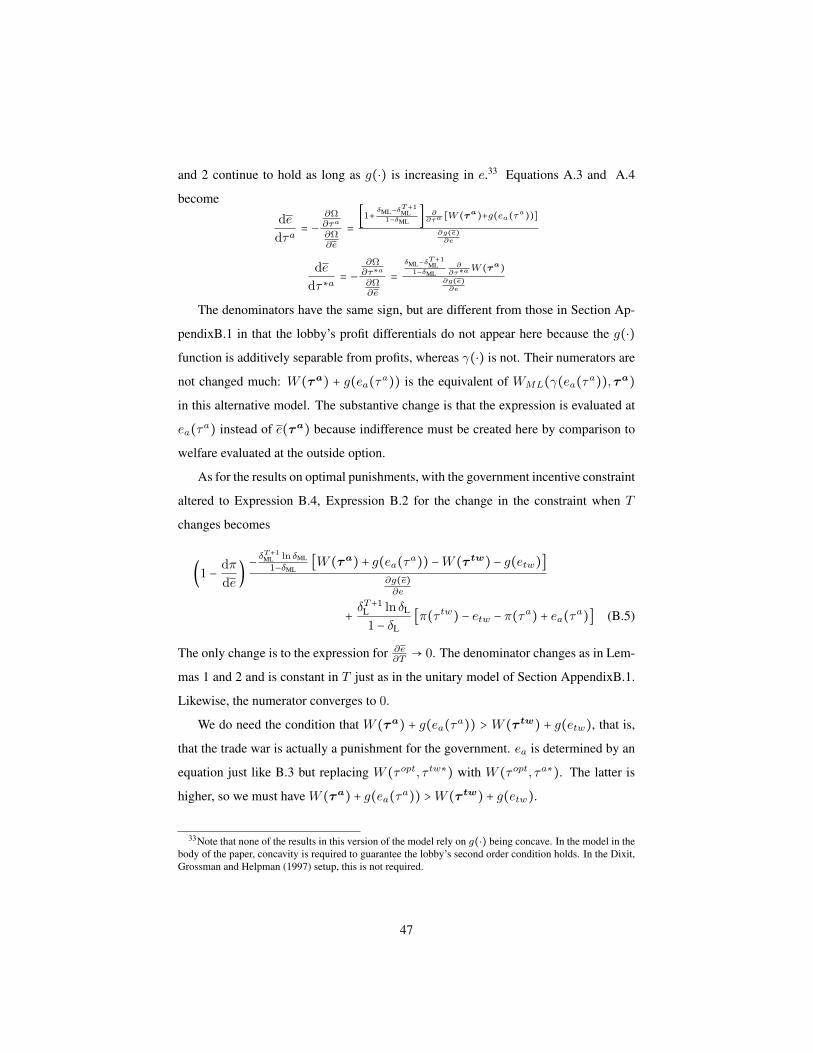
and 2 continue to hold as long as g(⋅) is increasing in e.33 Equations A.3 and A.4

become

de

dτa= −

∂Ω∂τa

∂Ω∂e

=[1+

δML−δT+1ML

1−δML]∂∂τa [W (τa

)+g(ea(τa))]

∂g(e)∂e

de

dτ∗a= −

∂Ω∂τ∗a∂Ω∂e

=δML−δT+1

ML1−δML

∂∂τ∗aW (τa

)

∂g(e)∂e

The denominators have the same sign, but are different from those in Section Ap-

pendixB.1 in that the lobby’s profit differentials do not appear here because the g(⋅)function is additively separable from profits, whereas γ(⋅) is not. Their numerators are

not changed much: W (τa) + g(ea(τa)) is the equivalent of WML(γ(ea(τa)),τa)in this alternative model. The substantive change is that the expression is evaluated at

ea(τa) instead of e(τa) because indifference must be created here by comparison to

welfare evaluated at the outside option.

As for the results on optimal punishments, with the government incentive constraint

altered to Expression B.4, Expression B.2 for the change in the constraint when T

changes becomes

(1 − dπ

de)− δ

T+1ML ln δML

1−δML[W (τa) + g(ea(τa)) −W (τ tw) − g(etw)]

∂g(e)∂e

+ δT+1L ln δL

1 − δL[π(τ tw) − etw − π(τa) + ea(τa)] (B.5)

The only change is to the expression for ∂e∂T→ 0. The denominator changes as in Lem-

mas 1 and 2 and is constant in T just as in the unitary model of Section AppendixB.1.

Likewise, the numerator converges to 0.

We do need the condition that W (τa) + g(ea(τa)) > W (τ tw) + g(etw), that is,

that the trade war is actually a punishment for the government. ea is determined by an

equation just like B.3 but replacing W (τopt, τ tw∗) with W (τopt, τa∗). The latter is

higher, so we must have W (τa) + g(ea(τa)) >W (τ tw) + g(etw).

33Note that none of the results in this version of the model rely on g(⋅) being concave. In the model in thebody of the paper, concavity is required to guarantee the lobby’s second order condition holds. In the Dixit,Grossman and Helpman (1997) setup, this is not required.

47

In order for a non-trivial trade agreement equilibrium to exist, that is, where τa <τ tw, it must be the case that there is a τa < τ tw at which the lobby loses money at

every (τ b, e) pair that is determined by Expression (B.4). As long as it is not prof-

itable for the lobby to induce a break at the pair that maximizes the lobby’s profit, this

condition is ensured. The conditions for the existence of a non-trivial trade agreement

are a bit simpler in the Dixit, Grossman and Helpman (1997)-style model because the

determination of τ b is more direct.

AppendixB.3. Strong Bindings

If the trade agreement involves strong bindings instead of tariff caps (i.e. weak

bindings), the legislature must deliver τa and the lobby’s optimal effort during a pe-

riod in which the trade agreement holds is ea = 0. That the lobby pays less—here,

nothing—for the protection it receives under the trade agreement is the only change

from the base model. This means that nothing changes in the trade war. Likewise the

legislature’s repeated-game incentive constraint is unchanged, and so Lemmas 1 and 2

are undisturbed by the change to strong bindings.

It is the lobby’s incentive constraint that changes since the lobby no longer pays

ea for the trade agreement tariff. This makes the lobby’s incentive constraint easier

to satisfy for strong bindings at a given τa. This can be seen in the next expression,

where the right-hand side of the incentive constraint becomes smaller:

eb ≥ π(τ b(eb)) − π(τa) + ea +δL − δT+1

L

1 − δL[π(τ tw) − etw − π(τa) + ea]

≥ π(τ b(eb)) − π(τa) +δL − δT+1

L

1 − δL[π(τ tw) − etw − π(τa)]

The lobby’s incentive constraint is still satisfied at τa = τn, so a solution always exists.

In order to have an interior solution, it must be that the lobby’s constraint is satisfied

before e(τa) reaches its peak or that e(τa) does not decrease too quickly after its peak

before the lobby’s constraint can be satisfied.

Because the change to strong bindings does not influence the legislature’s incentive

constraint, the e(τa) schedule is the same in the weak and strong bindings cases. In

both cases, as τa increases, net profits under the trade agreement increase. However,

they go up more under strong bindings. Because e(τa) is decreasing at the same rate in

48

both cases, a strong-binding agreement in which the lobby is not paying ea will satisfy

the constraint at a lower level of τa. For some parameter values, there will be a non-

trivial trade agreement under strong bindings but not under weak bindings. Intuitively,

for a given τa, the difference between net profits under a trade war and under the trade

agreement is smaller with a strong binding, so the incentive to break the agreement is

weaker under the strong-binding agreement.

Welfare comparisons here are nuanced. From the point of view of a welfare-

maximizing executive, welfare is higher under the strong-binding agreement because

lower trade agreement tariffs can be self-enforced.

The welfare comparison for the median legislator during the trade agreement phase

depends upon the comparison we make. Under the weak-binding agreement, the me-

dian legislator is chosen to match the tariff that will be applied, that is ea to match τa.

Under the strong-binding agreement, τa will still be applied, but the median legislator

is the one associated with e = 0 who prefers a lower tariff. Under the weak-binding

agreement, the tariff is politically efficient in that it matches the political-economy

weight of the decision maker. Under the strong-binding agreement, the tariff is no

longer politically efficient in this sense. Instead, there’s a mismatch between the tariff

and γ(0). The median legislator when bindings are weak would tend to experience a

reduction in welfare from a change to a strong-binding agreement because the trade

agreement tariff is being reduced below her optimal unilateral tariff; typically this re-

duction will not be outweighed by the increase in welfare of reducing the foreign tariff.

From the point of view of the median legislator under the strong binding—the legis-

lator identified by γ(0)—the strong-binding trade agreement tariff is unambiguously

better in welfare terms.

As in Maggi and Rodrıguez-Clare (2007), tariff caps in this model serve to keep the

lobby ‘in the game.’ A tariff cap makes the lobby’s self-enforcement constraint harder

to satisfy and thus requires a higher trade agreement tariff for self-enforcement. From

the ex-ante point of view, strong bindings are therefore preferable. Tariff caps could be

viewed as a way to commit to setting higher trade agreement tariffs and therefore as a

mechanism for ensuring that rents are distributed to protectionists ex-post.

49