Selection of Estimation Window in the Presence of

Breaks�

M. Hashem Pesaran

University of Cambridge and USC

Allan Timmermann

University of California, San Diego

Revised July, 2005, This version January 2006

Abstract

In situations where a regression model is subject to one or more breaks

it is shown that it can be optimal to use pre-break data to estimate the

parameters of the model used to compute out-of-sample forecasts. The issue

of how best to exploit the trade-o� that might exist between bias and fore-

cast error variance is explored and illustrated for the multivariate regression

model under the assumption of strictly exogenous regressors. In practice

when this assumption cannot be maintained and both the time and size of

the breaks are unknown the optimal choice of the observation window will be

subject to further uncertainties that make exploiting the bias-variance trade-

o� di�cult. To that end we propose a new set of cross-validation methods for

selection of a single estimation window and weighting or pooling methods for

combination of forecasts based on estimation windows of di�erent lengths.

Monte Carlo simulations are used to show when these procedures work well

compared with methods that ignore the presence of breaks.

JEL Classi�cations: C22, C53.

Key Words: Parameter instability, forecasting with breaks, choice of ob-

servation window, forecast combination.

�We would like to thank two anonymous referees and an associate editor for many excel-

lent suggestions on an earlier version of the paper. We also thank James Chu, David Hendry,

Adrian Pagan and seminar participants at Erasmus University at Rotterdam, London School of

Economics and University of Southern California for comments and discussion.

1. Introduction

Consider the multivariate regression model subject to a single structural break at

time t = T1

yt+1 = 1ft�T1g�01xt + (1� 1ft�T1g)�02xt + ut+1; t = 1; 2; :::; T: (1)

Here 1ft�T1g is an indicator variable that takes the value of one when t � T1, and

is zero otherwise, while xt is a p�1 vector of stochastic regressors, �i (i = 1; 2) arep�1 vectors of regression coe�cients, and ut+1 is a serially uncorrelated error termwith mean zero, assumed to be independently distributed of xt, possibly with a

shift in its variance from �21 to �22 at the time of the break. Assuming that �1 6= �2

or �21 6= �22; it follows that there is a structural break in the data generating process

at time T1 which we refer to as the break point.

Suppose that we know that � and/or � have changed at T1 and our interest lies

in forecasting yT+1 given the observations fyt; t = 1; :::; Tg and fxt; t = 1; :::; Tgwhich we collect in the information set T = fxt; ytgTt=1. How many observationsshould we use to estimate a model that, when used to generate forecasts, will

minimize the mean squared forecast error (MSFE)? Here we are not concerned

with the classical problem of identifying the exact point of the break, but rather

the sample size that it is optimal to use to estimate the parameters of the model

in order to forecast out-of-sample on the assumption that a structural break has in

fact occurred. The standard solution is to use only observations over the post-break

period (t = T1 + 1; :::; T ) to estimate the model.

We show in this paper that this solution need not be optimal when the objective

is to optimize forecasting performance. The intuition behind using pre-break data

is very simple in the case where the regressors are strictly exogenous. If structural

breaks characterize a particular time series, using the full historical data series to

estimate a forecasting model will lead to forecast errors that are no longer unbiased,

although they may have a lower variance. Provided that the break is not too large,

pre-break data will be informative for forecasting outcomes even after the break.

By trading o� the bias and forecast error variance, one can potentially improve on

the forecasting performance as measured by MSFE.

For the more general case where the regressors are not strictly exogenous, the

potential gains in forecasting performance from using pre-break data can readily

be demonstrated through Monte Carlo simulations. Not surprisingly, such gains

1

can be quite large if the time and the size of the break is known. In the more

common situation where these parameters are unknown, our simulations show that

forecasting accuracy can be improved by pre-testing for a structural break. How-

ever, the overall outcome crucially depends on how well the location of the break

point is estimated. In particular, information about the time of the break can be

important to forecasting performance even in the absence of knowledge about the

size of a break.

The main contributions of our paper are two-fold. First, we make a simple, yet

largely overlooked theoretical point, namely that when the objective is to minimize

out-of-sample MSFE it is often optimal to use pre-break data to estimate forecast-

ing models on data samples subject to structural breaks. To establish this point we

make a set of simplifying assumptions (such as strict exogeneity of the regressors)

which are unlikely to hold empirically but allow us to get a set of theoretical results

that are easy to understand. These assumptions also let us demonstrate analyt-

ically the factors determining the optimal estimation window both conditionally

and unconditionally.

Our second main contribution is to propose a set of new methods that facilitate

the practical implementation of the theoretical point that using pre-break data for

parameter estimation can lead to improved forecasting performance. Although our

paper focuses on the multivariate regression model, these methods are applicable

to general dynamic models and are hence useful in a wide set of circumstances.

It is commonplace to �nd that the timing of breaks as well as the size of any

shift in parameters are poorly estimated. For this reason the proposed methods

do not attempt to directly exploit the trade-o� between the bias and forecast error

variance but do so indirectly by searching across di�erent starting points for the

data window used to estimate the parameters of the forecasting model.

More speci�cally, we consider approaches based on cross-validation and forecast

combination (pooling) procedures. Cross-validation based on pseudo out-of-sample

forecasting performance can be used as a criterion for selecting estimation windows

of di�erent length. One approach is to simply choose a single window size that

leads to the lowest average out-of-sample loss over the cross-validation sample. This

may work well if the break is well-de�ned and large. Another approach, which is

likely to work better for relatively small breaks, is to combine forecasts based on

di�erent estimation windows, using equal weights or weights that are proportional

2

to the inverse of the out-of-sample loss. Such methods may or may not condition

on estimates of the break points and we consider both cases. Therefore, for this

latter approach we shall consider forecast combinations with alternative weighting

schemes and depending on whether knowledge of the breakpoints is used. This

approach is inspired by the forecast combination literature where forecasts from

alternative models are combined.1 Here we pool forecasts obtained using the same

model but estimated across di�erent observation windows. Clearly, a meta fore-

cast combination procedure that considers both sources of model uncertainty can

be entertained. The forecast combination strategy can also be seen as a risk di-

versi�cation strategy in the face of uncertainty regarding the breaks, and extends

concerns over model uncertainty to a wider class of models where regression equa-

tions subject to breaks are viewed as di�erent models.

The outline of the paper is as follows. Section 2 sets up the multivariate break-

point model and considers the choice of observation window for the conditional and

(for a simple data generating process) unconditional forecasting problem. Section

3 provides details of the implementation of the trade-o�, cross-validation and com-

bination methods. Section 4 reports Monte Carlo simulation results while Section

5 concludes.

2. Selection of the Optimal Window Size

Many tests for structural breaks have been proposed. In the context of linear

regression models Chow (1960) derived F-tests for structural breaks with a known

break point, while Brown, Durbin and Evans (1975) derived Cusum and Cusum

Squared tests that are also applicable when the time of the break is unknown. More

recently, contributions by Ploberger, Kramer and Kontrus (1989), Hansen (1992),

Andrews (1993), Inclan and Tiao (1994), Andrews and Ploberger (1996) and Chu,

Stinchcombe and White (1996) have extended tests for the presence of breaks to

account for heteroskedasticity and dynamics. Methods for estimating the size and

timing of multiple break points have also been developed, see Bai and Perron (1998,

2003) and Altissimo and Corradi (2003).

Less attention has been paid to the problem of determining the size of the

estimation window in the presence of breaks. To analyse this question, let m

1For reviews of the forecast combination literature see Clemen (1989), Granger (1989), Diebold

and Lopez (1996), and more recently Newbold and Harvey (2002) and Timmermann (2005).

3

denote the starting point of the sample of the most recent observations to be

used in estimation for the purpose of forecasting yT+1 based on the multivariate

regression model (1) and information T . Also, let Xm;T be the (T �m + 1) � p

matrix of observations on the regressors such that rank (Xm;T ) = p, while Ym;T

is the (T � m + 1) � 1 vector of observations on the dependent variable whosevalue for period T +1 we are interested in forecasting. De�ning the quadratic form

Q�;Ti = X0�;TiX�;Ti so that Q�;Ti = 0 if � > Ti, the OLS estimator of � based on

the sample from m to T (m < T � p+ 1) is given by

b�T (m) = Q�1m;TX

0m;TYm;T : (2)

The error in forecasting yT+1 from (1) will be a function of the data sample used

to estimate � and is given by

eT+1(m) = yT+1 � byT+1 = ��2 � b�T (m)�0 xT + uT+1: (3)

We implicitly assume that it is known that there is no break in the regression

model in period T + 1. Otherwise, the best forecast would need to consider the

distribution from which new regression parameters are drawn after a break.2

To derive analytical results, we assume that xt is strictly exogenous, in the

sense that it is independently distributed of us for all s and t, such that

E[xtjf(u1; u2; :::; uT+1)] = 0; for t = 1; :::; T (4)

where f(:) is a general function. In particular, it follows that E (xtjus) = 0, for

all t and s. While this assumption is clearly not empirically appropriate in many

situations, it simpli�es the analysis considerably and allows us to derive much

stronger and clearer results than would otherwise be possible.

Autoregressive processes subject to structural breaks have been considered by

Pesaran and Timmermann (2005). The advantage of that setup is that it is highly

relevant to many empirical situations, but the theoretical results are complicated to

interpret. Under strictly exogenous regressors, however, the factors determining the

optimal window length under breaks become very transparent. This case therefore

serves as a natural theoretical benchmark.

2A Bayesian procedure that allows for such a possibility is discussed in Pesaran, Pettenuzzo

and Timmermann (2004).

4

2.1. Conditional MSFE results

We shall consider the case where the prediction can be conditioned on the sequence

of xt values. Taking expectations of (3) conditional on XT = fx1;x2; :::;xTg, weget the conditional bias in the forecast error:

bias(mjXT ) � E[eT+1(m)jXT ] =��2 � b�T (m)�0 xT : (5)

Furthermore, using (2) it can be shown that

eT+1(m) =��02� Y0

m;TXm;TQ�1m;T

�xT + uT+1 (6)

= ( �2 � �1)0Qm;T1Q

�1m;TxT � u0m;TXm;TQ

�1m;TxT + uT+1;

where um;T = (um; um+1; ::; uT )0.

Squaring this expression and taking expectations, the conditional mean squared

forecast error (MSFE) given XT can be computed as follows:

MSFE(mjXT ) = E�e2T+1(m)jXT

�(7)

= �22 + �22��0Qm;T1Q

�1m;TxT

�2+x0TQ

�1m;TX

0m;T�m;TXm;TQ

�1m;TxT ;

where � = (�2��1)=�2, and �m;T = E�um;Tu

0m;T

�is a (T �m+1)� (T �m+1)

diagonal matrix with �21 on the �rst T1 � m + 1 diagonal places and �22 on the

remaining T � T1 places. Using (7) note that

MSFE(mjXT ) = �22(1 +Bm + Em) (8)

where Bm is the squared bias and Em the e�ciency term de�ned by

Bm = �0Qm;T1Q

�1m;TxTx

0TQ

�1m;TQm;T1�; (9)

and

Em = ��22 x0TQ

�1m;T

��21Qm;T1 + �22QT1+1;T

�Q�1m;TxT (10)

= x0TQ�1m;TxT +

�x0TQ

�1m;TQm;T1Q

�1m;TxT

�:

Here the (proportional) break in the innovation variance parameter is given by

= (�21 � �22) =�22. For a given value of xT , and 1 < m � T1 < T , it is clear that

since Qm;T �Qm+1;T = xm�1x0m�1 � 0; then

x0T�Q�1m;T �Q�1

m+1;T

�xT � 0; (11)

5

and similarly3

x0T�Q�1m;TQm;T1Q

�1m;T �Q�1

m+1;TQm+1;T1Q�1m+1;T

�xT � 0: (12)

The e�ciency gain of adding one more observation to the pre-break estimation

period (by reducing m) depends on whether �21 � �22 or �21 > �22. Under the former

inequality � 0, and using (11) and (12) in (10), it readily follows that

Em � Em+1 � 0; (13)

so that the forecast error variance is a decreasing function of the number of pre-

break data points used in model estimation. Under �21 > �22 the outcome is am-

biguous and we could have Em � Em+1 > 0:Letting Hm = Qm;T1Q

�1m;T , the change in the bias term from starting at obser-

vation m rather than observation m+ 1 is given by

Bm �Bm+1 = �0(HmxTx0TH

0m �Hm+1xTx

0THm+1)�:

Furthermore,

HmxTx0TH

0m �Hm+1xTx

0THm+1 = (Hm �Hm+1)xTx

0T (Hm �Hm+1)

+(Hm �Hm+1)xTx0THm+1

+Hm+1xTx0T (Hm �Hm+1)

0:

By Lemma 1 in Appendix A, Hm �Hm+1 � 0, and the matrices xTx0T ; Hm+1

are non-negative de�nite. Therefore

�0(HmxTx0TH

0m �Hm+1xTx

0THm+1)� � 0;

and so, irrespective of the sign of ,

Bm �Bm+1 � 0: (14)

This means that the squared bias always increases, the earlier the pre-break esti-

mation window is started.4

3Note that Qm;T1�Qm+1;T1 = xm�1x0m�1 � 0, and by assumption Qm;T is a positive de�nite

matrix.4In the absense of assumption (4) this result need not hold as discussed by Pesaran and

Timmermann (2005).

6

Consider now the overall change in MSFE(mjXT ) as the starting point of the

window is changed from m to m+ 1:

�m;m+1 = MSFE(mjXT )�MSFE(m+ 1jXT ) (15)

= �22 [(Bm �Bm+1) + (Em � Em+1)] :

When �21 � �22 (or � 0), using (13) and (14), it is clear that as m+1 is decreasedby one unit to m, �m;m+1 could rise or fall depending on whether the rise in Bm is

higher or lower than the potential fall in Em. Similarly, as m is reduced to m� 1,�m�1;m could either rise or fall. Therefore, MSFE(mjXT ) need not be monotonic

in m and there is a trade-o� between an increase in the bias Bm as m is reduced

compared to the potential increase in e�ciency which results in a reduction in Em.

In the case where �21 > �22 (and > 0) the sign of Em�Em+1 is ambiguous and itmight not be possible to reduce the MSFE by increasing the size of the pre-break

sample. These results suggest that it may be optimal to use pre-break data points,

particularly if �21 � �22. Appendix B presents a more formal analysis of when it

is optimal to use pre-break data to estimate the parameters of the multivariate

forecasting model.

For the univariate model (p = 1), some analytically tractable cases of special

interest emerge. If there is no break in the mean (� = 0) and �22 > �21, it is optimal

to use the full data set (and thus an expanding window) to estimate � although the

forecast error variance should be based on �22 and not on the weighted average of �21

and �22. In contrast, it is not optimal to include pre-break observations when either

�2 is very large or �21 is much larger than �22 so that is large. Hence if the break

in the mean parameters is high or the pre-break error variance is much higher than

the post-break error variance, then only post-break observations should be used

in the estimation. However, even if a sizeable break in the mean has occurred, it

may still be optimal to include pre-break data provided that the variance of the

regression equation is smaller before the break occurred.

Using v1 = T1�m+1 and v2 = T � T1 to denote the number of pre-break andpost-break observations, respectively, with v = v1+v2 being the total length of the

estimation window, we summarize our �ndings in the following proposition:

7

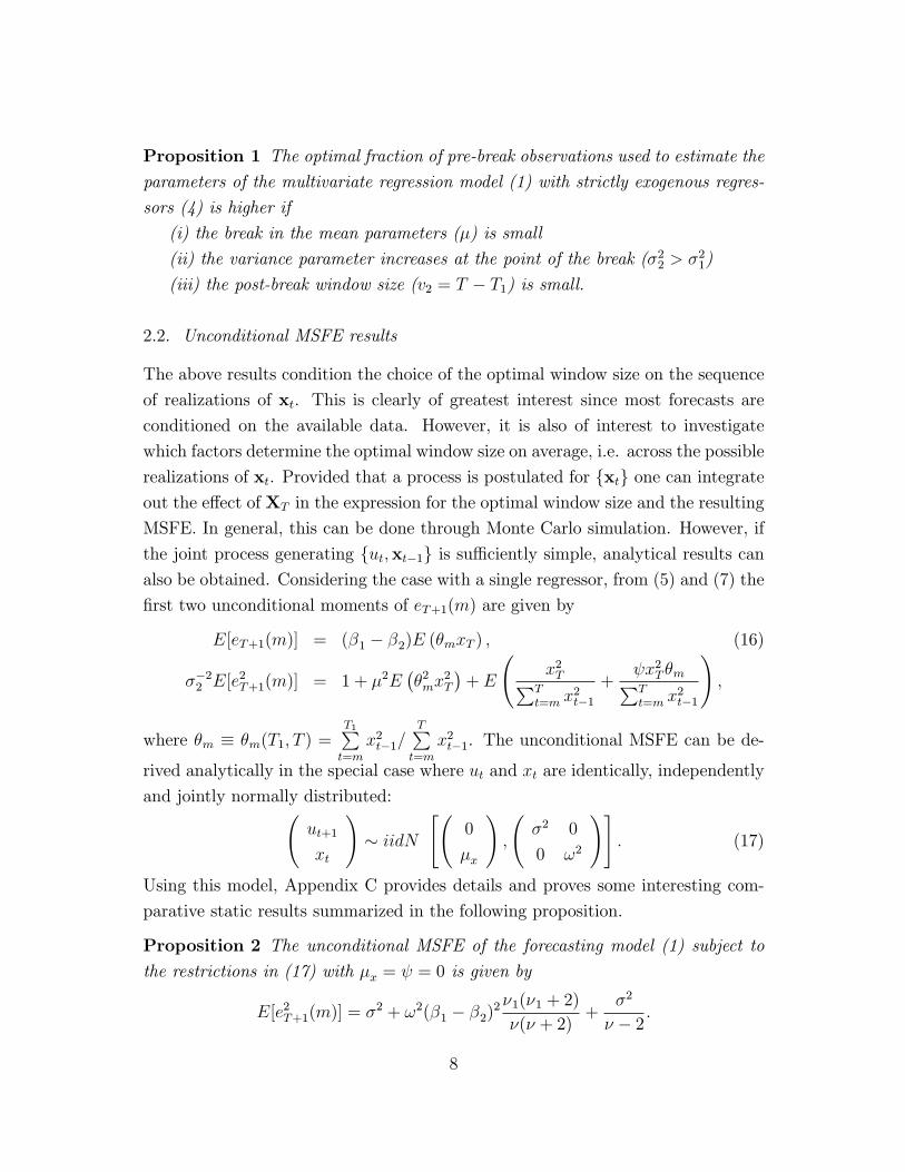
Proposition 1 The optimal fraction of pre-break observations used to estimate the

parameters of the multivariate regression model (1) with strictly exogenous regres-

sors (4) is higher if

(i) the break in the mean parameters (�) is small

(ii) the variance parameter increases at the point of the break (�22 > �21)

(iii) the post-break window size (v2 = T � T1) is small.

2.2. Unconditional MSFE results

The above results condition the choice of the optimal window size on the sequence

of realizations of xt. This is clearly of greatest interest since most forecasts are

conditioned on the available data. However, it is also of interest to investigate

which factors determine the optimal window size on average, i.e. across the possible

realizations of xt. Provided that a process is postulated for fxtg one can integrateout the e�ect of XT in the expression for the optimal window size and the resulting

MSFE. In general, this can be done through Monte Carlo simulation. However, if

the joint process generating fut;xt�1g is su�ciently simple, analytical results canalso be obtained. Considering the case with a single regressor, from (5) and (7) the

�rst two unconditional moments of eT+1(m) are given by

E[eT+1(m)] = (�1 � �2)E (�mxT ) ; (16)

��22 E[e2T+1(m)] = 1 + �2E��2mx

2T

�+ E

x2TPT

t=m x2t�1

+ x2T �mPTt=m x

2t�1

!;

where �m � �m(T1; T ) =T1Pt=m

x2t�1=TPt=m

x2t�1. The unconditional MSFE can be de-

rived analytically in the special case where ut and xt are identically, independently

and jointly normally distributed: ut+1

xt

!� iidN

" 0

�x

!;

�2 0

0 !2

!#: (17)

Using this model, Appendix C provides details and proves some interesting com-

parative static results summarized in the following proposition.

Proposition 2 The unconditional MSFE of the forecasting model (1) subject to

the restrictions in (17) with �x = = 0 is given by

E[e2T+1(m)] = �2 + !2(�1 � �2)2�1(�1 + 2)

�(� + 2)+

�2

� � 2 :

8

Hence the optimal pre-break window that minimizes the MSFE is longer

(i) the smaller the signal-to-noise ratio !2=�2

(ii) the smaller the size of the break (�1 � �2)2

(iii) the smaller the post-break window, v2.

The unconditional MSFE results are consistent with the conditional results

established previously and con�rm the intuition that the bene�ts from using more

pre-break data increases when breaks are small, di�cult to detect and occur late

in the sample.

3. Determination of Estimation window

In the context of the multivariate regression model with strictly exogenous re-

gressors the analytical results in Section 2 demonstrated the determinants of the

trade-o� involved in selecting the window used in estimating the parameters of

a forecasting model whose performance is evaluated on the basis of its out-of-

sample mean squared forecast error. While the multivariate regression model is in

widespread use in forecasting experiments, in many cases the strict exogeneity (4)

assumption cannot be maintained. Furthermore, in practical applications, neither

the time of any break(s), nor their size is likely to be known so one needs to consider

how to treat the uncertainty surrounding these in order to construct empirically

useful techniques.

To this end we consider in this section a broader class of strategies for deal-

ing with breaks in forecasting situations. The �rst strategy selects a single best

estimation window either by adopting cross-validation methods to a pseudo out-

of-sample forecasting experiment, by exclusively using post-break data or by using

the (in-sample) trade-o� embedded in equation (30). The second strategy bor-

rows ideas from the literature on forecast combinations and combines forecasts

from models estimated on di�erent observation windows using a variety of robust

weighting schemes. This strategy has the advantage that it bypasses the need for

direct estimation of breakpoint parameters�a task that is often di�cult in practice,particularly when it comes to determining the timing of small breaks, c.f. Elliott

(2005). Another advantage to this approach is that it is applicable to general dy-

namic models and for estimation methods other than least squares such as the

maximum likelihood or the generalized method of moments.

9

Common to all methods is that the estimation window should exceed a mini-

mum length, !: This assumption is not necessarily restrictive since ! can always

be set equal to a very small number, i.e. the number of regressors plus one. In

practice, however, to account for the very large e�ect of parameter estimation er-

ror in cases with few data points per estimated parameter, ! should be reasonably

large, say at least 2-3 times the number of unknown parameters. Furthermore,

those forecasting methods that rely on cross-validation reserve the last ~! observa-

tions to measure pseudo out-of-sample forecasting performance used in ranking or

weighting the various models.

We next provide speci�c details on the implementation of each approach. For

simplicity we discuss the approaches under the assumption of a single break, but the

generalization to multiple breaks is straightforward. For those approaches that pre-

test for a break, we shall assume that an estimate of the breakpoint, T1, is available

using methods such as those proposed by Bai and Perron (1998) or Altissimo and

Corradi (2003).

3.1. Post-Break Window

Suppose that the forecaster has an estimate of the time of the break, T1. A simple

estimation strategy is then to only use post-break data [T1+1 : T ] to estimate the

parameters of the model, denoted �T1+1:T , where �T1+1:T =�PT

j=T1+1xj�1x

0j�1

��1�PT

j=T1+1x0j�1yj, and the resulting forecast is computed as yT+1(T1) = �

0T1+1:T

xT .

This strategy only involves estimating the time of the break and thus does not

require the estimation of pre-break parameters or the post-break variance.

3.2. Trade-o� Method

The trade-o� function is given by (30) in Appendix B, and is speci�ed in terms of

� = v1=v, the fraction of the pre-break observations. An estimate of the optimum

value of �, which we denote by ��, is given by

��= argmin

�

(�2��0�v1�

�1v xT

�2+�

v

�x0T �

�1v �v1�

�1v xT

�+1

v

�x0T �

�1v xT

�);

(18)

10

subject to 0 � ��< 1, where5

�v = ��v1 + (1� �)�v2 ; = (�21 � �22)=�

22; � = (�2 � �1)=�2;

�1 =

0@ T1Xt=1

xt�1x0t�1

1A�1T1Xt=1

x0t�1yt, �2 =

0@ TXt=T1+1

xt�1x0t�1

1A�1TX

t=T1+1

x0t�1yt;

�v1 = T�11

0@ T1Xt=1

xt�1x0t�1

1A ; �v2 = (T � T1)�1

0@ TXt=T1+1

xt�1x0t�1

1A ;

T1 is an estimate of the time of the break, and

�21 = (T1� p� 1)�1T1Xt=1

(yt�x0t�1�2)2; �22 = (T � T1� p� 1)�1TX

t=T1+1

(yt�x0t�1�2)2:

We shall refer to estimation windows determined in this way as based on the

trade-o� method since it attempts to trade-o� bias against reduction in parameter

estimation error.

If both the pre- and post-break window sizes, v1 and v2, were to go to in�nity,

under broad conditions and � could be consistently estimated. However, in most

economic applications�and the ones that concern us here�even if the number ofpre-break observations is very large, the number of post-break data points, v2, is

likely to be small and as a result it would not be possible to estimate �� consistently

so other approaches that deal with the uncertainty that surrounds �� need to be

considered.

3.3. Cross-Validation

The cross-validation approach reserves the last ~! observations of the data for an

out-of-sample estimation exercise and chooses the estimation window that gener-

ates the smallest MSFE value on this sample. Since we further assume that a

minimum of ! observations is needed to estimate the parameters of the forecasting

5To simplify the derivation of ��, we abstract from the dependence of �v1 on v1, and instead

use the pre-break observations to estimate �v1 . Similarly, the structural parameters, � and ,

are also based on pre- and post-break data.

11

model, this means that !+~! data points are required to adopt this method. For

each potential starting point of the estimation window, m, the recursive pseudo

out-of-sample MSFE value is computed as:

MSFE (mjT; ~!) = ~!�1T�1X

�=T�~!(y�+1 � x0� �m:� )2; (19)

where �m:� is the OLS estimate based on the observation window [m; � ]. Suppose

again that the forecaster has an estimate of the time of the break, T1 and de�ne

m�(T; T1; !; ~!) as that value of m 2 1; :::; T1 + 1, or m 2 1; :::; T�!�~! (whicheveris smallest since on e�ciency grounds it would only be meaningful to search for

windows that start prior to T1 + 1) that minimizes the out-of-sample MSFE:

m��T; T1; !; ~!

�= arg min

m=1;:::; min(T1+1;T�!�~!)

(~!�1

T�1X�=T�~!

(y�+1 � x0� �m:� )2):

(20)

The corresponding forecast for period T + 1 is computed as

yT+1

�T; T1;m

��= x0T �m�:T :

This approach can readily be implemented without an estimate of T1, treating the

break date as unknown. In this case the optimal break date is determined from

m� (T; !; ~!) = arg minm=1;:::; T�!�~!

(~!�1

T�1X�=T�~!

(y�+1 � x0� �m:� )2); (21)

so this method searches for m� along the points m = 1; :::; T � !� ~! regardless ofthe break date.

3.4. Weighted Average Combination

In many empirical applications, as argued by Elliott (2005) and Paye and Timmer-

mann (2004), it can be di�cult to obtain a precise estimate of the time and size of

a potential break. In particular, when the length of the evaluation sample (~!) is

short, the estimate of m� is likely to be subject to considerable uncertainty. Rather

than selecting a single (poorly determined) estimation window, it becomes attrac-

tive to combine forecasts based on di�erent estimation windows. One approach

that builds on ideas from the forecast combination literature is to let the forecast

12

combination weights be proportional to the inverse of the associated out-of-sample

MSFE values. Suppose again that an estimate of the break date, T1, is available

and assume that T1 + 1 < T � ~!�!.6 Then the combined (weighted) forecast isgiven by:

yT+1;W

�T; T1; ~!

�=

PT1+1m=1

�x0T �m:T

�MSFE (mjT; ~!)PT1+1

m=1 MSFE (mjT; ~!): (22)

The only point where knowledge of the time of the break (T1) is assumed in (22) is

in determining the set from which m� is selected. Values of m greater than T1 + 1

lead to ine�cient estimators since they do not make use of all data points after the

most recent break and can thus be disregarded.

Once again, this approach can be extended to treat the break date as unknown

to avoid the need for having an estimate of T1 and simply combine the optimal

forecasts allowing for the minimal estimation and evaluation windows !; ~!. In this

case all values of m 2 1; :::; T � ! � ~! are considered and the weighted average

forecast is given by:

yT+1;W (T; !; ~!) =

PT�!�~!m=1

�x0T �m:T

�MSFE (mjT; ~!)PT�!�~!

m=1 MSFE (mjT; ~!): (23)

3.5. Simple Average Combination (Pooled Forecast)

A particularly simple combination approach is to put equal weights on all forecasts

generated subject to m � T1 + 1 (or, more speci�cally, m � min(T1 + 1; T � !)):

yT+1

�T; T1; !

�= (T1 + 1)

�1T1+1Xm=1

x0T �m:T ; (24)

Alternatively, when an estimate, T1, is not available, subject to utilizing a minimal

window length, !:

yT+1 (T; !) = (T � !)�1T�!Xm=1

x0T �m:T : (25)

These forecasts build on the common �nding in the literature on forecast combina-

tion that equal-weighted forecasts perform quite well and are di�cult to beat, c.f.

Clemen (1989) and Stock and Watson (2001).

6In general, the summation in (22) runs from m = 1; :::;min(T1 + 1; T � ~!�!).

13

3.6. Multiple Breaks

For simplicity, so far only the possibility of a single break is assumed, but in practice

a time-series model may be subject to multiple breaks. The presence of multiple

breaks complicates the relationship between the (squared) bias and forecast error

variance since more breakpoint scenarios become possible. For example, under

two breaks the parameters may be trending upwards or downwards across break

segments (making early data less useful for estimation) or alternatively be mean-

reverting (making early data useful but more recent data less so). Clearly, the

trade-o� between using one pre-break data point versus none at all does not hinge

on the absence of multiple breaks. However, things get more complicated once

more than one pre-break data point is included. Consider, for example, the case

where a break happened at time T1 and another at time T1 � 1. While inclusionof two data points may have been optimal in the absence of the additional break

at time T1 � 1, this could be overturned if this break (assuming that it could bedetected) generated data from a model su�ciently di�erent from that prevailing

after time T1.

Although the theoretical results get more complicated, the presence of multiple

breaks need not complicate application of the above methods which extend in

obvious ways. Formulas such as (21), (23) and (25) do not rely on an estimate of

the timing (or size) of breaks which only indirectly show up in the patterns observed

in the MSFE-values computed as a function of the window length. Furthermore,

since the e�ciency argument of using all post-break data only applies to the data

after the most recent break, in the presence of multiple breaks one can use the

cross-validation or trade-o� methods as in (18) and (20) but (in the latter case)

computing out-of-sample MSFE-values either for m = 1; :::; Tb + 1 (in cases where

earlier breaks are either believed to be di�cult to detect or of a su�ciently small

magnitude) or m 2 Tb�1 + 1; :::; Tb + 1, where Tb�1 and Tb are the estimated datesof the penultimate and ultimate breaks.

3.7. Discussion

Although we focus on the multivariate regression model, the approaches proposed in

this paper can readily be extended to handle di�erent types of estimators required

14

for general dynamic models of the form

yt+1 = g(xt;�) + "t+1; (26)

where g(:) is a general nonlinear function. They can also be readily adapted to use

with general loss functions L(yt+1; yt+1) in addition to the quadratic loss that is

commonly used and that we have adopted here.

The combination and cross-validation approaches do not depend on precise esti-

mation of the size of the pre- and post-break parameters and, as we have seen, also

do not necessarily require having an estimate of the time of the break(s), although

it is an option to use such information when available. This is a disadvantage in

the sense that they do not trade o� the e�ects described in Section 2. However,

the trade-o�s can be di�cult to exploit in practice given the uncertainty surround-

ing the parameters characterizing any break(s), so in practice this may not be too

much of a concern.

These methods require choosing the two parameters ! and ~!, the length of the

minimal estimation window and the length of the evaluation window (although

the pooling approach only requires the former). Choosing ! is not much of an

issue and is simply a feature that robusti�es the combination methods against the

in uence of extreme forecasts that could result when the number of data points

used to estimate a forecasting model is very small. Selection of ~! is driven by

the usual considerations faced by researchers attempting to partition a sample

into in-sample and out-of-sample periods. If ~! is set too large, then too much

smoothing may result and forecasting methods that performed well earlier during

the sample may be preferred over models that perform better closer to the end

point, T . Conversely, if ~! is set too short, then the ranking of forecasting models

will be too noisy and a�ected too greatly by random variations. In our simulations

we set ! at 10% and ~! at 25% of the sample, but other values could of course be

used.

To obtain an estimate of the time of the break we shall use the method proposed

by Bai and Perron (1998, 2003). This approach provides consistent estimates of

the number of breaks under a broad set of conditions and (most importantly)

allows for multiple breaks. The method can be implemented in several ways. We

use the Schwarz Information Criterion to select the number of breaks, allow for

up to three breaks and require a minimum of ten observations between successive

15

breaks (the simulation results are not sensitive to this assumption). Alternative

approaches for detecting multiple structural breaks are also available. For example,

Altissimo and Corradi (2003) propose a strongly consistent approach to estimating

the number of breaks sequentially which asymptotically lets the probability of over-

and underestimating the number of breaks converge to zero. They further propose

a small sample correction to detecting the number of breaks which is demonstrated

to perform well in Monte Carlo experiments.

In the case with a single break, the time of the break, T1, can be consistently

estimated under the conditions established by Bai (1997). Since it is not optimal

for estimation purposes to only use part of the post-break sample [T1 + 1; T ], it

follows that expressions such as (20) and (21), (22) and (23), (24) and (25) will be

pair-wise asymptotically equivalent. This, of course, requires that the number of

pre- and post-break observations is very large, a condition that is unlikely to hold

in practice in many situations.

4. Monte Carlo Simulations

Our simulation setup assumes that data is generated according to a bivariate

VAR(1) model yt

xt

!=

�yt�xt

!+At

yt�1

xt�1

!+

"yt

"xt

!; (27)

where var("yt) = �2"yt; var("xt) = �2"xt and cov("yt; "xt) = 0. The approach is

general enough to relax these distributional assumptions and higher order dynamics

can readily be accommodated by viewing (27) as being in companion form and

letting xt be a p� 1 vector of predictor variables.Breaks to the conditional mean are parameterized as follows:

At =

8>>>><>>>>:

a11 a12

0 a22

!t � T1

a11 + d11 a12 + d12

0 a22 + d22

!t > T1

: (28)

This setup is similar to that adopted in Clark and McCracken (2001, 2005). In this

parameterization, the values of dij indicate the size of a break. Breaks in A occur

at time T1 + 1 and a�ect the conditional distribution of yt given yt�1 and xt�1.

16

a21 is always normalized at zero so x Granger-causes y; but not the reverse. We

start the process from its pre-break stationary distribution and assume that while

the mean parameters are a�ected by breaks, the unconditional or long-run mean

is una�ected by breaks, i.e. �t = (I�At)�1�0 for t � T1 + 1, and �0 denotes the

pre-break unconditional mean.

In the Monte Carlo simulations with no break to the variance we set �"y =

�"x = 1 and cov("yt; "xt) = 0. Breaks to the conditional variance are introduced

by letting

�"yt =

(1 t � T1

� t > T1;

where � > 0 is a scaling factor that indicates a higher post-break variance if � > 1

and a lower post-break variance if � < 1.

To account for the importance of the position of the break in relation to the

sample size, we consider a range of combinations of the break date and sample size

by letting the break occur at 25%, 50% and 75% of the full sample size. The latter

is varied from 100 to 200 observations.

As a natural benchmark we consider forecasts from a model that ignores breaks

and uses all observations�this is an optimal estimation window in situations withno breaks. MSFE-values are reported relative to those produced by this benchmark,

so a value of unity means the same MSFE performance as the benchmark, values

above unity suggest worse forecasting performance and values below unity indicate

better forecasting performance than the benchmark.

The parameter values assumed in the Monte Carlo experiments are shown in

Table 1. Experiment 1 considers the case without a break. Experiment 2 introduces

a relatively small break of -0.2 in the autoregressive parameter, a11 that declines

from 0.9 to 0.7 after the break, while experiment 3 assumes that this break is

somewhat larger at -0.4. Experiments 4 and 5 consider the e�ect of small and large

breaks to the marginal coe�cient of xt�1 on yt by letting a12 change from 1 to

1.5 or 2 after the break. Experiment 6 studies the e�ect of a simultaneous break

to a11 which declines from 0.9 to 0.7 and an increase in a12 from 1 to 2. Finally,

experiments 7 and 8 change the volatility parameter by letting �"y increase from 1

to 4 (experiment 7) or decrease from 1 to 0.5 (experiment 8).

Table 2 reports the MSFE-values for one-step-ahead forecasts computed at the

end of the sample using the methods introduced in Section 3. Results are based

17

on 5,000 Monte Carlo simulations. For comparison we also show MSFE results for

the infeasible post-break, cross-validation, weighted average and trade-o� methods

under the assumption that the time of the break, T1, though not its size, is known.

For experiment 1, that assumes there are no breaks, the forecasting method

that generates the lowest out-of-sample MSFE-value is the expanding window.

This is unsurprising in view of its e�ciency properties in the absence of a break so

that the longer the estimation window, the better. However, the various window

determination methods also perform quite well�only the cross-validation approachand the pooling method that treat any break points as unknown generate e�ciency

losses of two or three percent.

Turning to the simulations under breaks (experiments two through eight), in

experiment 2 where the autoregressive root of y goes from 0.9 to 0.7 at the time of

the break, the ranking between the forecasting methods changes signi�cantly. Now

the full-sample estimator performs worst among all the methods, followed by the

weighted average method that conditions on an estimate of the time of the break,

T1. In contrast, the cross-validation and pooled forecasting methods perform very

well�nearly as well as the infeasible post-break or cross-validation methods thatcondition on the true value of T1. The trade-o� method performs in line with the

post-break method.

When the size of the break to the AR(1) parameter of the predicted variable is

increased (experiment 3), the cross-validation methods continue to perform best,

independently of whether a pre-test for the break is undertaken. When measured

against the full sample method, the performance of all methods that incorporate

break point information improves as one would expect.

Under a small break to a12 (experiment 4), the best feasible methods are the two

combination methods that do not pre-test for a break. The pooling method does

particularly well across di�erent values of the time of the break, T1. As the break in

a12 gets larger (experiment 5), the ranking changes and the approach that pre-tests

for a break date followed by cross-validation across the dates m = 1; :::; T1 + 1 is

best followed closely by the post-break and trade-o� methods that also pre-test for

a break. The post-break and trade-o� methods perform well across di�erent break

dates, while the performance of the cross-validation approach deteriorates when T1

gets close to T . These three methods are also best under a simultaneous break to

a11 and a12 (experiment 6).

18

There is a simple explanation for these �ndings. When a break is large it

becomes easier to detect and so using a pre-test to obtain an estimate of the time

of the break leads to improved forecasting performance. Conversely, when a break

is relatively small, it is better to treat the timing of the break as unknown and not

attempt to estimate pre- and post-break parameters.

These observations can be con�rmed from Table 3 which reports the average

window sizes selected by a variety of methods. Panel A shows that when the size of

the break is small (experiment 4), both the cross-validation and trade-o� methods

based on an estimate of T1 use too long window sizes: When T1 = 25, on average

the window should be close to 75 observations, but instead it is 87 observations for

these methods. This re ects a di�culty in detecting a relatively small break�theaverage estimate of T1 for this experiment is 16 observations, well below the true

value of 25. As the break gets larger (experiment 6), the average window length

increases to 78-79 observations, only a little higher than the post-break window

of 75 observations. This is consistent with break date estimates that average 24

observations for experiments 5 and 6.

Another point that is worth noting is that as the time of the break approaches

the end of the sample (i.e. T1 = 75), the performance of the cross-validation

and weighted average methods that pre-test for a break and consider estimation

windows starting at m = 1; :::; T1 + 1 deteriorates. In both cases this is related

to the imprecision in estimating the time of the break and (in the case of the

weighted average forecast) to averaging over too many models that use too long

a data sample for estimation purposes. In contrast, the post-break, trade-o� and

pooling methods (the latter assuming an unknown break date) perform quite well

in these experiments. This happens for a subtle reason. When T1 is close to the

end of the sample, T , the true post-break window (v2 = T � T1) is short and

so the results in Section 2 suggest that it is optimal to use relatively many pre-

break observations. This e�ect is important for both the post-break and trade-o�

approaches that use close to 40 observations when the break is large (experiments

5 and 6) due in part to the fact that the Bai-Perron method tends to underestimate

the time of the break (the average value of T1 in these experiments is 62, below the

true value of 75).

While the post-break method based on an estimated value of T1 generally per-

forms quite well, it performs poorly when a break only a�ects the variance of the

19

time series (experiments 7 and 8) and the Bai-Perron method fails to detect this

break. Hence it is mainly in situations where a break is believed to a�ect the con-

ditional mean that this method can be recommended.7 In general, when the break

is con�ned to the error variances forecasts based on expanding (`full') estimation

window seem to perform best.

The weighted average method combined with a pre-break test appears to be the

superior method when the conditional mean is not subject to a break. Conversely,

this method performs rather poorly when such a break occurs (in experiments 2-6).

The explanation for this �nding is again related to the estimates of the break dates.

The average estimate of the break date is close to zero when a break either is not

present or only a�ects the variance of the time series. In contrast, the weighted

average that treats the time of the break as unknown performs better under breaks

to the mean. Since this method averages over more models estimated on post-break

data only (when the break occurs after 25 periods), it appears that the e�ciency

loss associated with using too few post-break observations (resulting from treating

T1 as unknown) is less important than the squared bias e�ect due to con�ning the

averaging to models estimated on pre-break data. When the time of the break gets

larger relative to the cross-validation window (~!), the performance of the weighted

average method that treats T1 as unknown also deteriorates.

The timing of the break (T1 = 25; 50; 75) has some impact on the performance of

the various approaches. Among the methods that attempt to estimate the time of

a possible break, the relative performance of the post-break and trade-o� methods

improves as the time of the break increases. Among the methods that treat the

time of a break as unknown, the pooled method performs relatively well when the

break occurs either early (T1 = 25) or late (T1 = 75) during the sample, while

the cross-validation approach performs best when a break occurs in the middle of

the sample (T1 = 50). This �nding of a great deal of sensitivity in out-of-sample

forecasting performance to the timing of the break is mirrored by the analysis of

Clark and McCracken (2005).

As the sample size gets larger (panels D-F in Table 2), the performance of the

methods that test for a break systematically improves relative to the expanding

window approach. Part of the reason for this lies in the improved precision of the

estimates of the time of the break which for experiments 5 and 6 vary between 98

7Alternatively, a di�erent method for detecting breaks to the variance should be adopted.

20

and 99 observations (the true value being 100). As a result, the post-break method

generally performs rather well as does the trade-o� method.

We conclude the following from these simulations. First, which method is best

depends on the setup of the simulation experiment�in particular, the timing, sizeand nature of the break. Second, under a break to the coe�cients determining the

conditional mean of the predicted variable, an approach that pre-tests for a break

and uses a set of inverse-MSE weights to compute a weighted average performs

distinctly worse than the other approaches considered here. Third, an approach

that pre-tests for a break and only uses post-break data generally performs well as

does the cross-validation and pooling approaches that treat the size of the break

as unknown. Fourth, the trade-o� approach that determines the number of pre-

break data points to include by trading o� the squared bias against the reduction

in forecast error variance, generally leads to slightly higher out-of-sample MSFE

values compared to a simple post-break approach that ignores pre-break data. The

reasons for this �nding are clear. For a start, it is generally di�cult to determine

precisely the date of the break�something which is crucial when determining theoptimal trade-o�. Furthermore, and linked to the �rst point, estimates of the pre-

break and post-break parameters�needed to determine the break size�are againplagued by errors and this will infect the trade-o�. Even so, the trade-o� method

does improve on the post-break method in cases where the break only a�ects the

variance. In general, however, an approach that uses estimates of a possible break

date and then applies cross-validation to determine the estimation window appears

to be a more robust way to proceed.

4.1. Results with Multiple Breaks

To account for the possibility of multiple breaks we also considered experiments

with two breaks occurring at time T1 and T2, respectively. We assumed that the

breaks occur at one- and two-thirds of the sample, respectively. Under this setup

there are three break segments so the AR coe�cients can now either decline, in-

21

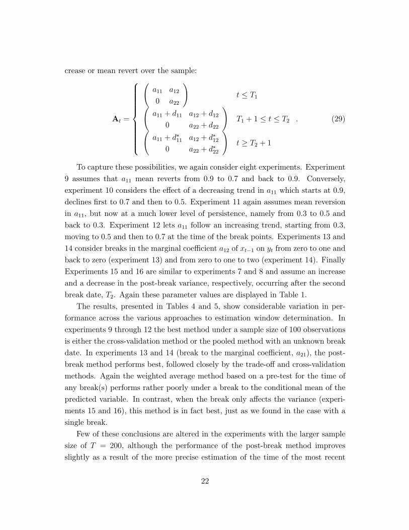
crease or mean revert over the sample:

At =

8>>>>>>>>><>>>>>>>>>:

a11 a12

0 a22

!t � T1

a11 + d11 a12 + d12

0 a22 + d22

!T1 + 1 � t � T2

a11 + d�11 a12 + d�120 a22 + d�22

!t � T2 + 1

: (29)

To capture these possibilities, we again consider eight experiments. Experiment

9 assumes that a11 mean reverts from 0.9 to 0.7 and back to 0.9. Conversely,

experiment 10 considers the e�ect of a decreasing trend in a11 which starts at 0.9,

declines �rst to 0.7 and then to 0.5. Experiment 11 again assumes mean reversion

in a11, but now at a much lower level of persistence, namely from 0.3 to 0.5 and

back to 0.3. Experiment 12 lets a11 follow an increasing trend, starting from 0.3,

moving to 0.5 and then to 0.7 at the time of the break points. Experiments 13 and

14 consider breaks in the marginal coe�cient a12 of xt�1 on yt from zero to one and

back to zero (experiment 13) and from zero to one to two (experiment 14). Finally

Experiments 15 and 16 are similar to experiments 7 and 8 and assume an increase

and a decrease in the post-break variance, respectively, occurring after the second

break date, T2. Again these parameter values are displayed in Table 1.

The results, presented in Tables 4 and 5, show considerable variation in per-

formance across the various approaches to estimation window determination. In

experiments 9 through 12 the best method under a sample size of 100 observations

is either the cross-validation method or the pooled method with an unknown break

date. In experiments 13 and 14 (break to the marginal coe�cient, a21), the post-

break method performs best, followed closely by the trade-o� and cross-validation

methods. Again the weighted average method based on a pre-test for the time of

any break(s) performs rather poorly under a break to the conditional mean of the

predicted variable. In contrast, when the break only a�ects the variance (experi-

ments 15 and 16), this method is in fact best, just as we found in the case with a

single break.

Few of these conclusions are altered in the experiments with the larger sample

size of T = 200, although the performance of the post-break method improves

slightly as a result of the more precise estimation of the time of the most recent

22

break with a larger sample size. In fact, in experiments 13 and 14 the average

estimates of the second break date is 131, close to the true value of 132, while in

the smaller sample of 100 observations the corresponding estimates were 62, a bit

below the true value of 66.

5. Conclusion

When interest lies in forecasting time-series with regression models that are subject

to structural breaks, one might think that the parameters of the forecasting model

should be estimated exclusively on data available after the most recent break.

However, such an approach ignores two important facts. First, as we show in

this paper, in choosing the estimation window there is in general an important

trade-o� between bias and forecast error variance which means that it is generally

advantageous to include (some) pre-break information. Second, it can be di�cult to

precisely estimate the timing of one or multiple breaks, particularly when these are

small and/or occur close to the boundaries of the data sample. It also follows from

this point that, in practice, it is generally di�cult to optimally exploit the bias-

variance trade-o� to determine the window size since the parameters characterizing

the break points are imprecisely determined. Our results suggest that while little

is lost by attempting to exploit the trade-o� when the breaks only a�ect the error

variances, the trade-o� approach can improve on an approach that estimates the

model parameters only on post-break data.

As a result of di�culties in estimating the time and size of the break(s), we

proposed a range of alternative methods that either rely on pseudo out-of-sample

cross-validation or use forecast combination methods to combine forecasts from

models whose parameters are estimated using di�erent window sizes. These meth-

ods can be implemented without any knowledge of breaks to the underlying para-

meters. For many break processes we found that combination and pooling methods

work well, particularly when the break is su�ciently small and hence di�cult to

detect.

Our �ndings are closely related to the work by Clark and McCracken (2005) on

how the power of tests of predictive ability are a�ected by structural breaks. Clark

and McCracken �nd that structural breaks can severely a�ect the out-of-sample

predictive performance of econometric models. It follows from this work that re-

searchers should be very careful in how they set up the out-of-sample forecasting

23

experiment, paying close attention to any evidence of breaks. This is consistent

with our results that estimation methods that display di�erent degrees of sensi-

tivity to structural breaks tend to produce very di�erent out-of-sample forecasting

performance.

Appendix A

Lemma 1: Let Hm = Qm;T1Q�1m;T ; where Qm;T = X

0m;TXm;T =

PTt=m xt�1x

0t�1

and 1 � m < T1 < T . Then

Hm �Hm+1 � 0,

where � denotes a positive semi-de�nite matrix.Proof of Lemma 1. Note that

Hm �Hm+1 = (xm�1x0m�1 +Qm+1;T1)Q

�1m;T �Qm+1;T1Q

�1m+1;T :

Multiplying by Q�1m;T = (xm�1x

0m�1+Qm+1;T ) and rearranging, we have that Hm >

Hm+1 if

xm�1x0m�1 +Qm+1;T1 > Qm+1;T1Q

�1m+1;Txm�1x

0m�1 +Qm+1;T1

or equivalently if

(Qm+1;TQ�1m+1;T �Qm+1;T1Q

�1m+1;T )xm�1x

0m�1 > 0:

This holds provided that

(Qm+1;T �Qm+1;T1)Q�1m+1;Txm�1x

0m�1 > 0

which is satis�ed here sinceQm+1;T�Qm+1;T1 =PT

t=T1+1xt�1x

0t�1 > 0 and xm�1x

0m�1,

Qm+1;T are non-negative de�nite matrices.

Appendix B

This appendix considers determinants of whether it is optimal to use pre-break

data to estimate the parameters of the multivariate regression model. Recall that

Qm;T =PT1

t=m xt�1x0t�1 +

PTt=T1+1

xt�1x0t�1, and de�ne

�v = v�1Qm;T =�v1v

��v1 +

�v2v

��v2 ;

24

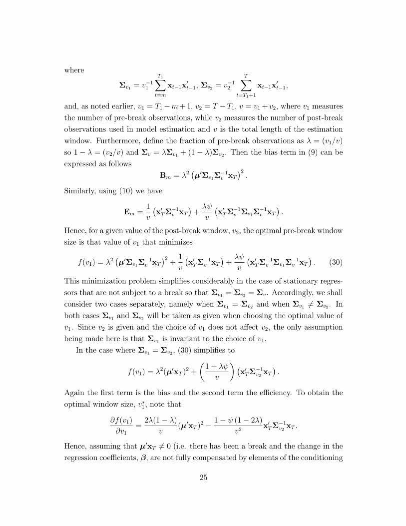
where

�v1 = v�11

T1Xt=m

xt�1x0t�1, �v2 = v�12

TXt=T1+1

xt�1x0t�1;

and, as noted earlier, v1 = T1�m+1; v2 = T �T1; v = v1+ v2, where v1 measures

the number of pre-break observations, while v2 measures the number of post-break

observations used in model estimation and v is the total length of the estimation

window. Furthermore, de�ne the fraction of pre-break observations as � = (v1=v)

so 1� � = (v2=v) and �v = ��v1 + (1� �)�v2 . Then the bias term in (9) can be

expressed as follows

Bm = �2��0�v1�

�1v xT

�2:

Similarly, using (10) we have

Em =1

v

�x0T�

�1v xT

�+�

v

�x0T�

�1v �v1�

�1v xT

�:

Hence, for a given value of the post-break window, v2, the optimal pre-break window

size is that value of v1 that minimizes

f(v1) = �2��0�v1�

�1v xT

�2+1

v

�x0T�

�1v xT

�+�

v

�x0T�

�1v �v1�

�1v xT

�: (30)

This minimization problem simpli�es considerably in the case of stationary regres-

sors that are not subject to a break so that �v1 = �v2 = �v. Accordingly, we shall

consider two cases separately, namely when �v1 = �v2 and when �v1 6= �v2 . Inboth cases �v1 and �v2 will be taken as given when choosing the optimal value of

v1. Since v2 is given and the choice of v1 does not a�ect v2, the only assumption

being made here is that �v1 is invariant to the choice of v1.

In the case where �v1 = �v2 ; (30) simpli�es to

f(v1) = �2(�0xT )2 +

�1 + �

v

��x0T�

�1v2xT�:

Again the �rst term is the bias and the second term the e�ciency. To obtain the

optimal window size, v�1, note that

@f(v1)

@v1=2�(1� �)

v(�0xT )

2 � 1� (1� 2�)v2

x0T��1v2xT :

Hence, assuming that �0xT 6= 0 (i.e. there has been a break and the change in theregression coe�cients, �, are not fully compensated by elements of the conditioning

25

vector, xT ),

�� =v�1

v�1 + v2=

(1� )

2 (v2RT � ); (31)

where

RT =(�0xT )

2

x0T��1v2xT

> 0:

Note that since x0T��1v2xT > 0; f(v1) can also be written as

f(v1) = x0T�

�1v2xT

��2RT +

�1 + �

v

��;

and in the case where � = 0 (RT = 0), and = 0, we have f(v1) = (v1 +

v2)�1 �x0T��1v2 xT �. Hence, in the absence of breaks, as to be expected, the min-

imum value of f(v1) is achieved for a maximum value of v1.8

The solution in (31) is feasible if 0 � �� < 1. To ensure that the inclusion of

pre-break data is optimal it is further required that �� > 0; and @2f(v1)=@2v1 > 0

when evaluated at v�1. As noted above an optimal feasible solution is guaranteed

only in the case where � 0. In this case clearly �� > 0 and since

@2f(v1)

@2v1= 2

�x0T�

�1v2xT� �(1� �)(1� 3�)

v2RT +

1� (2� 3�)v3

�;

when evaluated at �� we have9�x0T�

�1v2xT��1 @2f(v�1)

@2v1=

(2v2RT � 1� ) (2v2RT � 3 + ) v2RT2 (v2RT � )2 v2v2

+2

v3

� (4v2RT � 3� )

(v2RT � ) v3:

In the special case where �21 = �22 the above results simplify considerably. For

�� we have

�� =1

2v2RT=x0T�

�1v2xT

2v2(�0xT )2:

This shows that the optimal fraction of the pre-break window depends inversely

on the post-break window size and the \e�ective" break size, j�0xT j. It also variesdirectly with x0T�

�1v2xT which is likely to be of order p, the number of regressors.

8Once again recall that v2 is given and does not vary with v1.9When � 0, the second-order condition @2f(v�1)=@

2v1 > 0 will be satis�ed if v2(�0xT )

2 >32

�x0T�

�1v2 xT

�, namely if the break size is su�ciently large.

26

This analysis can also be readily extended to the case where �v1 6= �v2 , so longas we continue to assume that �v1 does not vary with v1. Under this assumption

and using (30) we have

@f(v1)

@v1=

2�(1� �)

v

��0�v1�

�1v xT

�2+ 2�2

��0�v1�

�1v xT

���0�v1

@��1v@v1

xT

�� 1v2�x0T�

�1v xT

�+1

v

�x0T@��1v@v1

xT

�+ (1� 2�)

v2�x0T�

�1v �v1�

�1v xT

�+2�

v

�x0T@��1

v

@v1�v1�

�1v xT

�;

where@��1v@v1

= �1� �

v��1v (�v1 ��v2)�

�1v :

In this case the optimal choice of v1 or � is a complicated function of �v1 and �v2but can be readily obtained using numerical techniques.

Appendix C

In this appendix we derive the unconditional MSFE expression used in Propo-

sition 2. First, notice that under assumption (17),

E�x2T �

2m

�= E

�x2T�E��2m�:

Furthermore,

�m ��2�1(�1)

�2�1(�1) + �2�2(�2); (32)

where the total window size, � = T �m + 1; is split into a pre-break window size

�1 = T1�m+1; and a post-break window size �2 = T�T1. �2�1(�1) is a non-centralchi-squared distribution with non-centrality parameter �1 = �1�

2x and �1 degrees of

freedom. Likewise, �2�2(�2) is a non-central chi-squared distribution (independent

of �2�1(�1)) with non-centrality parameter �2 = �2�2x and �2 degrees of freedom.

Hence �m follows a doubly non-central beta distribution with parameters �1=2 and

�2=2 and non-centrality parameters �1 and �2. Using a result due to Patnaik

(1949), the �rst two moments of �m are approximately given by

E (�m) t�1

�1 + �2=�1�< 1 (33)

E��2m�t

��1�

� (1 + k�1)(1 + k�)

;

27

where k = (1 + 2�2x)2=(2 + 8�2x). Assuming that = 0 (�21 = �22 = �2), so that

there is only a break in the conditional mean, the expected value of the last term

in (16) can be shown to be given by

E

x2TPT

t=m x2t�1

!=

�1

2

�exp(�1

2�)(1 + �2)� (34)

1Xj=0

(12�)j

j!

�(12(� � 2) + j)�(1

2� + j)

;

where � = ��2x and � = �x=!. This expression can easily be evaluated numerically.

Hence the unconditional MSFE is approximately given by

E[e2T+1(m)] t �2 + (�1 � �2)2(!2 + �2x)

��1�

� (1 + k�1)(1 + k�)

+

��2

2

�exp(�1

2�)(1 + �2)�

1Xj=0

(12�)j

j!

�(12(� � 2) + j)�(1

2� + j)

:

Tractable exact analytical results can be obtained when it is further assumed that

�x = 0: In this case the non-centrality parameters are zero,

�m � Beta(�12;�22);

and the �rst two moments of �m are now given exactly by

E (�m) =�1�;

E��2m�=

�1(�1 + 2)

�(� + 2):

Also,

E

x2TPT

t=m x2t�1

!=

1

� � 2 ;

and, unconditionally,

E (�mxT ) = E (xT )E (�m) = 0:

In total, we obtain the following expression for the unconditional MSFE:

E[e2T+1(m)] = �2 + !2(�1 � �2)2�1(�1 + 2)

�(� + 2)+

�2

� � 2 : (35)

28

References

Altissimo and V. Corradi, 2003, Strong Rules for Detecting the Number of

Breaks in a Time Series. Journal of Econometrics 117, 207-244.

Andrews, D.W.K., 1993, Tests for Parameter Instability and Structural Change

with Unknown Change Point. Econometrica 61, 821-856.

Andrews, D.W.K. and W. Ploberger, 1996, Optimal Changepoint Tests for

Normal Linear Regression. Journal of Econometrics 70, 9-38.

Bai, J., 1997, Estimation of a Change Point in Multiple Regression Models.

Review of Economics and Statistics 79, 551-563.

Bai, J. and P. Perron, 1998, Estimating and Testing Linear Models with Mul-

tiple Structural Changes. Econometrica 66, 47-78.

Bai, J. and P. Perron, 2003, Computation and Analysis of Multiple Structural

Change Models, Journal of Applied Econometrics, 18, pp. 1-22.

Brown, R.L., J. Durbin, and J.M. Evans, 1975, Techniques for Testing the

Constancy of Regression Relationships over Time. Journal of the Royal Statistical

Society, Series B, 37, 149-192.

Chow, G., 1960, Tests of Equality Between Sets of Coe�cients in Two Linear

Regressions. Econometrica 28, 591-605.

Chu, C-S J., M. Stinchcombe, and H.White, 1996 Monitoring Structural Change.

Econometrica 64, 1045-1065.

Clark, T.E. and M.W. McCracken, 2001, Tests of Equal Forecast Accuracy and

Encompassing for Nested Models. Journal of Econometrics 105, 85-110.

Clark, T.E. and M.W. McCracken, 2005, The Power of Tests of Predictive

Ability in the Presence of Structural Breaks. Journal of Econometrics 124, 1-31.

Clemen, R. T., 1989, Combining Forecasts: A Review and Annotated Bibliog-

raphy, International Journal of Forecasting, 5, 559-583.

Diebold, F.X. and J.A. Lopez, 1996, Forecast Evaluation and Combination, in

G. S. Maddala and C. R. Rao (eds.), Handbook of Statistics, Volume 14, 241-268.

North-Holland, Elsevier: Amsterdam.

Elliott, G., 2005, Forecasting in the presence of a break. Mimeo, UCSD.

Granger, C., 1989, Combining forecasts - Twenty years later, Journal of Fore-

casting, 8, 167|173.

Hansen, B.E., 1992, Tests for Parameter Instability in Regressions with I(1)

Processes. Journal of Business and Economic Statistics 10, 321-335.

29

Inclan, C. and G.C. Tiao, 1994, Use of Cumulative Sums of Squares for Ret-

rospective Detection of Changes of Variance. Journal of the American Statistical

Association 89, 913-923.

Newbold, P. and D. I. Harvey, 2002, Forecasting combination and encompassing.

In M. P. Clements and D. F. Hendry (Eds.), A Companion to Economic Forecasting,

pp. 268{83. Oxford: Blackwell.

Patnaik, P.B. (1949) The non-central �2� and F�Distributions and their ap-plications. Biometrika 36, 202-232.

Paye, B. and A. Timmermann, 2004, Instability of Return Prediction Models.

Forthcoming in Journal of Empirical Finance.

Pesaran, M.H. and A. Timmermann, 2005, Small Sample Properties of Forecasts

from Autoregressive Models under Structural Breaks. Journal of Econometrics 129,

183-217.

Pesaran, M.H., D. Pettenuzzo, and A. Timmermann, 2004, Forecasting Time

Series Subject to Multiple Structural Breaks. Forthcoming in Review of Economic

Studies.

Ploberger, W., W. Kramer, and K. Kontrus, 1989, A New Test for Structural

Stability in the Linear Regression Model. Journal of Econometrics 40, 307-318.

Stock, J.H. and M. Watson, 2001, A Comparison of Linear and Nonlinear Uni-

variate Models for Forecasting Macroeconomic Time Series. Pages 1-44 In R.F.

Engle and H. White (eds). Festschrift in Honour of Clive Granger.

Timmermann, A, 2005, Forecast Combinations. Forthcoming in Elliott, G.,

C.W.J. Granger and A. Timmermann (Eds.), Handbook of Economic Forecasting,

North Holland.

30

Table 1: Simulation Setup I. Single Break

Experiment no: d11 d12 d22 σy Comments 1 0 0 0 1 no break 2 -0.2 0 0 1 small break in AR(1) dynamics 3 -0.4 0 0 1 large break in AR(1) dynamics 4 0 0.5 0 1 small break in marginal coefficient 5 0 1 0 1 large break in marginal coefficient 6 -0.2 1 0 1 break in dynamics, marginal coefficient 7 0 0 0 4 increase in post-break variance 8 0 0 0 0.5 decrease in post-break variance

II. Multiple Breaks

Experiment no: a11 d11 d12 d11* d12* σy Comments 9 0.9 -0.2 0 0 0 1 mean reversion in AR dynamics

10 0.9 -0.2 0 -0.4 0 1 decreasing trend in AR dynamics 11 0.3 0.2 0 0 0 1 mean reversion in AR dynamics 12 0.3 0.2 0 0.4 0 1 increasing trend in AR dynamics 13 0.9 0 1 0 0 1 mean reverting break in marginal coefficient 14 0.9 0 1 0 2 1 trended break in marginal coefficient 15 0.9 0 0 0 0 4 increase in post-break variance 16 0.9 0 0 0 0 0.5 decrease in post-break variance

Note: Under a single break it is assumed that a11 = 0.9. In both sets of experiments, a12 = 1, a22 = 0.9, a21 = 0 and d21 = d22 = 0. See Section 4 for details of the Monte Carlo experiments.

Table 2: MSFE-Values Under a Single Structural Break Known Break date Estimated break date Unknown break date full post cross- weighted pooled Trade-off post cross- weighted pooled Trade-off cross- weighted pooled Panels sample break validation average break validation average validation average A: 10,25~,25,100 1 ==== ωωTT Exp. # 1 1 -- -- -- -- -- 1.017 1.006 1.001 1.002 1.017 1.032 1.014 1.030

2 1 0.717 0.728 0.850 0.831 0.720 0.740 0.733 0.861 0.845 0.744 0.739 0.744 0.736 3 1 0.560 0.569 0.809 0.771 0.562 0.592 0.570 0.819 0.787 0.597 0.579 0.623 0.584 4 1 0.911 0.924 0.941 0.938 0.915 0.957 0.945 0.955 0.954 0.960 0.943 0.919 0.931 5 1 0.702 0.714 0.829 0.803 0.707 0.719 0.718 0.834 0.810 0.723 0.730 0.734 0.725 6 1 0.717 0.730 0.837 0.815 0.718 0.733 0.734 0.843 0.824 0.735 0.744 0.744 0.737 7 1 1.019 1.008 1.007 1.007 1.011 1.036 1.009 1.002 1.003 1.035 1.030 1.020 1.034 8 1 1.004 1.004 0.998 0.998 1.003 1.005 1.003 1.001 1.001 1.005 1.026 1.006 1.022

B: 10,25~,50,100 1 ==== ωωTT Exp. # 1 1 -- -- -- -- -- 1.017 1.006 1.001 1.002 1.017 1.032 1.014 1.030

2 1 0.603 0.618 0.835 0.808 0.610 0.630 0.626 0.847 0.822 0.640 0.623 0.761 0.666 3 1 0.455 0.465 0.816 0.771 0.458 0.486 0.464 0.824 0.784 0.500 0.469 0.722 0.554 4 1 0.803 0.822 0.875 0.867 0.808 0.862 0.859 0.902 0.894 0.868 0.833 0.844 0.825 5 1 0.478 0.486 0.739 0.682 0.484 0.487 0.488 0.745 0.690 0.498 0.493 0.670 0.546 6 1 0.536 0.546 0.772 0.730 0.541 0.546 0.548 0.778 0.737 0.555 0.553 0.702 0.596 7 1 1.060 1.019 1.015 1.014 1.040 1.104 1.017 1.005 1.007 1.096 1.033 1.023 1.039 8 1 1.030 1.015 1.001 1.000 1.034 1.006 1.004 1.001 1.002 1.006 1.026 1.003 1.017

C: 10,25~,75,100 1 ==== ωωTT Exp. # 1 1 -- -- -- -- -- 1.017 1.006 1.001 1.002 1.017 1.032 1.014 1.030

2 1 0.568 0.815 0.884 0.814 0.592 0.649 0.831 0.897 0.842 0.686 0.815 0.884 0.732 3 1 0.410 0.777 0.878 0.794 0.435 0.479 0.779 0.881 0.811 0.531 0.777 0.878 0.677 4 1 0.750 0.828 0.873 0.825 0.767 0.863 0.877 0.910 0.880 0.876 0.828 0.873 0.791 5 1 0.369 0.559 0.764 0.647 0.395 0.400 0.564 0.767 0.661 0.429 0.559 0.764 0.563 6 1 0.453 0.666 0.838 0.741 0.478 0.487 0.671 0.841 0.756 0.514 0.666 0.838 0.651 7 1 1.174 1.030 1.017 1.024 1.136 1.207 1.017 1.005 1.010 1.191 1.030 1.017 1.038 8 1 1.136 1.024 1.010 1.009 1.123 1.008 1.003 1.002 1.002 1.008 1.024 1.010 1.017

Notes: The experiments are defined in Table 1. T is the total sample size, T1 is the break point, ω~ is the size of the evaluation window and ω is size of the minimum estimation window. All MSFE’s are reported relative to the associated MSFE based on the full sample. Table continued….

Table 2(Continued): MSFE-Values Under a Single Structural Break Known Break date Estimated break date Unknown break date full post cross- weighted pooled Trade-off post cross- weighted pooled Trade-off cross- weighted pooled sample break validation average break validation average validation average Panels D: 20,50~,50,200 1 ==== ωωTT Exp. # 1 1 -- -- -- -- -- 1.002 1.000 1.000 1.000 1.001 1.020 1.009 1.016

2 1 0.671 0.676 0.837 0.817 0.672 0.674 0.676 0.842 0.822 0.675 0.684 0.708 0.688 3 1 0.518 0.522 0.812 0.773 0.518 0.530 0.522 0.818 0.782 0.531 0.527 0.596 0.542 4 1 0.916 0.923 0.943 0.941 0.918 0.924 0.925 0.946 0.944 0.925 0.933 0.922 0.926 5 1 0.710 0.717 0.823 0.802 0.711 0.711 0.717 0.826 0.806 0.713 0.724 0.736 0.723 6 1 0.684 0.689 0.814 0.793 0.685 0.686 0.689 0.817 0.796 0.687 0.696 0.712 0.698 7 1 1.009 1.004 1.004 1.004 1.003 1.013 1.001 1.000 1.000 1.012 1.021 1.011 1.018 8 1 1.004 1.004 1.000 1.000 1.004 1.000 1.000 1.000 1.000 1.000 1.018 1.006 1.013

E: 20,50~,100,200 1 ==== ωωTT Exp. # 1 1 -- -- -- -- -- 1.002 1.000 1.000 1.000 1.001 1.020 1.009 1.016

2 1 0.545 0.550 0.825 0.794 0.547 0.549 0.550 0.830 0.800 0.552 0.553 0.744 0.623 3 1 0.417 0.422 0.823 0.779 0.418 0.433 0.422 0.827 0.786 0.436 0.424 0.725 0.532 4 1 0.786 0.792 0.870 0.860 0.787 0.795 0.795 0.873 0.864 0.799 0.797 0.836 0.807 5 1 0.457 0.461 0.726 0.667 0.459 0.460 0.461 0.729 0.671 0.463 0.464 0.657 0.521 6 1 0.481 0.484 0.765 0.717 0.486 0.485 0.484 0.768 0.721 0.490 0.488 0.688 0.554 7 1 1.030 1.009 1.008 1.008 1.017 1.053 1.004 1.001 1.002 1.050 1.016 1.012 1.020 8 1 1.019 1.011 1.002 1.002 1.019 1.000 1.000 1.000 1.000 1.000 1.017 1.004 1.011

F: 20,50~,150,200 1 ==== ωωTT Exp. # 1 1 -- -- -- -- -- 1.002 1.000 1.000 1.000 1.001 1.020 1.009 1.016

2 1 0.484 0.708 0.878 0.802 0.492 0.499 0.709 0.879 0.810 0.513 0.708 0.878 0.702 3 1 0.357 0.683 0.867 0.783 0.364 0.380 0.683 0.867 0.790 0.398 0.683 0.867 0.654 4 1 0.668 0.750 0.871 0.815 0.679 0.704 0.761 0.878 0.827 0.713 0.750 0.871 0.764 5 1 0.314 0.476 0.775 0.652 0.322 0.319 0.476 0.775 0.656 0.331 0.476 0.775 0.548 6 1 0.393 0.594 0.847 0.749 0.399 0.399 0.595 0.847 0.755 0.413 0.594 0.847 0.639 7 1 1.089 1.017 1.010 1.014 1.064 1.192 1.011 1.005 1.009 1.171 1.017 1.010 1.020 8 1 1.066 1.018 1.008 1.009 1.056 0.999 1.000 1.000 1.000 0.999 1.018 1.008 1.011

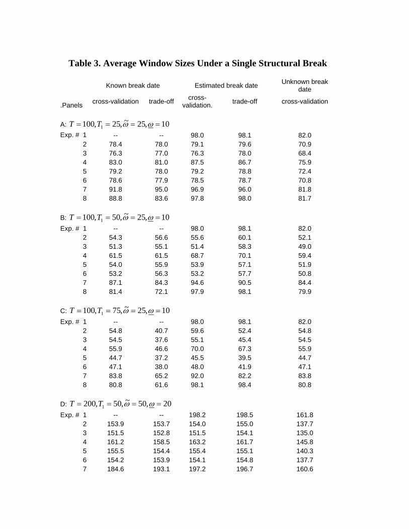
Table 3. Average Window Sizes Under a Single Structural Break

Known break date Estimated break date Unknown break date

.Panels cross-validation trade-off cross-validation. trade-off cross-validation

A: 10,25~,25,100 1 ==== ωωTT Exp. # 1 -- -- 98.0 98.1 82.0

2 78.4 78.0 79.1 79.6 70.9 3 76.3 77.0 76.3 78.0 68.4 4 83.0 81.0 87.5 86.7 75.9 5 79.2 78.0 79.2 78.8 72.4 6 78.6 77.9 78.5 78.7 70.8 7 91.8 95.0 96.9 96.0 81.8 8 88.8 83.6 97.8 98.0 81.7

B: 10,25~,50,100 1 ==== ωωTT Exp. # 1 -- -- 98.0 98.1 82.0

2 54.3 56.6 55.6 60.1 52.1 3 51.3 55.1 51.4 58.3 49.0 4 61.5 61.5 68.7 70.1 59.4 5 54.0 55.9 53.9 57.1 51.9 6 53.2 56.3 53.2 57.7 50.8 7 87.1 84.3 94.6 90.5 84.4 8 81.4 72.1 97.9 98.1 79.9

C: 10,25~,75,100 1 ==== ωωTT Exp. # 1 -- -- 98.0 98.1 82.0

2 54.8 40.7 59.6 52.4 54.8 3 54.5 37.6 55.1 45.4 54.5 4 55.9 46.6 70.0 67.3 55.9 5 44.7 37.2 45.5 39.5 44.7 6 47.1 38.0 48.0 41.9 47.1 7 83.8 65.2 92.0 82.2 83.8 8 80.8 61.6 98.1 98.4 80.8

D: 20,50~,50,200 1 ==== ωωTT Exp. # 1 -- -- 198.2 198.5 161.8

2 153.9 153.7 154.0 155.0 137.7 3 151.5 152.8 151.5 154.1 135.0 4 161.2 158.5 163.2 161.7 145.8 5 155.5 154.4 155.4 155.1 140.3 6 154.2 153.9 154.1 154.8 137.7 7 184.6 193.1 197.2 196.7 160.6

8 177.5 166.2 197.9 198.0 161.8 Table 3 Continued E: 20,50~,100,200 1 ==== ωωTT Exp. # 1 -- -- 198.2 198.5 161.8

2 103.3 110.2 103.4 112.0 98.5 3 101.2 109.1 101.4 111.7 96.0 4 111.0 115.9 111.6 117.8 106.3 5 104.0 109.0 104.0 110.3 99.2 6 103.2 108.8 103.3 110.3 98.0 7 174.2 173.9 193.0 185.7 167.8 8 160.2 143.7 198.1 198.5 156.4

F: 20,50~,150,200 1 ==== ωωTT Exp. # 1 -- -- 198.2 198.5 161.8

2 87.4 70.8 88.6 77.5 87.4 3 86.3 68.1 86.3 75.0 86.3 4 86.7 78.7 95.0 91.0 86.7 5 75.7 66.1 75.8 68.2 75.7 6 77.8 67.9 77.8 70.1 77.8 7 165.6 136.9 183.6 156.0 165.6 8 158.9 129.8 198.3 198.7 158.9

The experiments are defined in Table 1. T is the total sample size; T1 is the break point, ω~ is the size of the evaluation window and ω is size of the minimum estimation window. The reported window sizes are averages of the windows selected across 5,000 replications.

Table 4: MSFE-Values Under Multiple Breaks

Known break date Estimated break date Unknown break date

full post cross- weighted pooled Trade-off post cross- weighted pooled Trade-

off cross- weighted pooled

sample break validation average break validation average validation average Panels A: 10,25~,66,33,100 21 ===== ωωTTT Exp.# 9 1 0.906 0.934 1.015 0.991 0.915 0.949 0.946 1.011 0.986 0.959 0.934 1.015 0.939

10 1 0.512 0.533 0.695 0.639 0.517 0.576 0.559 0.783 0.741 0.580 0.533 0.695 0.575 11 1 0.989 1.001 1.005 1.000 0.998 1.015 1.004 1.004 1.003 1.013 1.001 1.005 0.980 12 1 0.740 0.759 0.813 0.796 0.746 0.795 0.790 0.853 0.836 0.799 0.759 0.813 0.761 13 1 0.702 0.766 1.049 0.982 0.736 0.744 0.768 1.051 0.989 0.779 0.766 1.049 0.837 14 1 0.213 0.225 0.571 0.420 0.220 0.223 0.227 0.580 0.432 0.233 0.225 0.571 0.324 15 1 1.120 1.030 1.020 1.021 1.092 1.176 1.016 1.007 1.011 1.161 1.030 1.020 1.039 16 1 1.079 1.026 1.006 1.005 1.070 1.009 1.005 1.002 1.002 1.009 1.026 1.006 1.016

B: 20,50~,132,66,200 21 ===== ωωTTT Exp. # 9 1 0.886 0.906 1.039 1.015 0.896 0.895 0.906 1.041 1.015 0.909 0.906 1.039 0.948

10 1 0.464 0.472 0.690 0.629 0.466 0.492 0.490 0.731 0.675 0.494 0.472 0.690 0.550 11 1 0.947 0.965 1.006 1.001 0.950 0.997 0.992 1.005 1.003 0.998 0.965 1.006 0.968 12 1 0.711 0.719 0.811 0.790 0.716 0.733 0.728 0.830 0.809 0.737 0.719 0.811 0.748 13 1 0.657 0.681 1.076 1.006 0.663 0.662 0.682 1.077 1.011 0.671 0.681 1.076 0.837 14 1 0.189 0.194 0.576 0.422 0.193 0.191 0.194 0.577 0.426 0.195 0.194 0.576 0.314 15 1 1.063 1.015 1.012 1.012 1.044 1.135 1.008 1.005 1.008 1.129 1.015 1.012 1.021 16 1 1.045 1.017 1.005 1.006 1.043 1.000 1.000 1.000 1.000 1.000 1.017 1.005 1.010

Notes: The experiments are defined in Table 1. T is the total sample size, T1 and T2 give the position of the first and the second break points, ω~ is the size of the evaluation window and ω is size of the minimum estimation window. All MSFE’s are reported relative to the associated MSFE based on the full sample.

Table 5: Average Window Sizes Under Multiple Breaks

Known break date Estimated break date Unknown break

Panels cross-validation trade-off cross-validation trade-off cross-

validation. A: 10,25~,66,33,100 21 ===== ωωTTT Exp. # 9 67.4 53.8 73.2 44.9 67.4

10 47.3 56.7 55.4 57.3 47.3 11 68.9 52.6 92.7 55.2 68.9 12 51.3 51.1 59.5 56.3 51.3 13 54.1 55.0 55.5 41.3 54.1 14 39.4 56.3 40.2 41.1 39.4 15 84.9 56.4 92.9 35.5 84.9 16 79.7 60.1 98.0 71.4 79.7

B: 20,50~,132,66,200 21 ===== ωωTTT Exp. # 9 113.2 100.3 115.5 80.9 113.2

10 79.6 108.5 89.1 92.3 79.6 11 115.8 95.6 170.0 98.3 115.8 12 84.9 91.4 92.4 100.0 84.9 13 83.2 109.2 83.3 76.9 83.2 14 73.2 111.8 73.3 75.9 73.2 15 168.8 115.1 188.1 56.0 168.8 16 156.5 119.8 198.3 152.2 156.5

Notes: The experiments are defined in Table 1. T is the total sample size, T1 and T2 give the position of the first and the second break points, ω~ is the size of the evaluation window and ω is size of the minimum estimation window.