ECONOMIC GROWTH CENTERYALE UNIVERSITY

P.O. Box 208629New Haven, CT 06520-8269

http://www.econ.yale.edu/~egcenter/

CENTER DISCUSSION PAPER NO. 944

Selection and Comparative Advantagein Technology Adoption

Tavneet SuriMassachusetts Institute of Technology

September 2006

Notes: Center Discussion Papers are preliminary materials circulated to stimulate discussions and criticalcomments.

MIT Sloan, email: tavneet@mit.edu. I am extremely grateful to Michael Boozer for countless hoursof discussion on this project. I would also like to thank the rest of my committee, Gustav Ranis, PaulSchultz and Christopher Udry, as well as Robert Evenson, Fabian Lange and seminar audiences atYale and NEUDC for comments. A special thanks to Thom Jayne and Margaret Beaver at MichiganState University for help with the 1997-2002 rounds of the data. I am sincerely grateful to theTegemeo Institute and Thom Jayne for including me in the 2004 survey and especially to Tegemeofor their hospitality during the field work in Kenya. I would like to thank James Nyoro, Director ofTegemeo, as well as Tegemeo Research Fellows Miltone Ayieko, Joshua Ariga, Paul Gamba andMilu Muyanga, Senior Research Assistant Frances Karin, and Research Assistants Bridget Ochieng,Mary Bundi, Raphael Gitau, Sam Mburu, Mercy Mutua and Daniel Kariuki and all the field teamsfor their impressive work through all the rounds of the survey, especially 2004. An additional thanksto Margaret Beaver and Daniel Kariuki for spending immense energy ensuring the data was squeakyclean. The data come from the Tegemeo Agricultural Monitoring and Policy Analysis (TAMPA)Project, between Tegemeo Institute at Egerton University, Kenya and Michigan State University,funded by USAID, April 1996 - June 2005. Any rainfall data used come from the Climate PredictionCenter and are part of the USAID/FEWS project - thanks to Tim Love for his repeated help withthese data.

This paper can be downloaded without charge from the Social Science Research Networkelectronic library at: http://ssrn.com/abstract=933124

An index to papers in the Economic Growth Center Discussion Paper Series is located at:http://www.econ.yale.edu/~egcenter/research.htm

Selection and Comparative Advantage in Technology Adoption

Tavneet Suri

ABSTRACT

This paper examines a well known empirical puzzle in the literature on technology adoption: despitethe potential of technologies to increase returns dramatically, a significant fraction of householdsdo not use these technologies. I study the use of hybrid maize and fertilizer in Kenya, where thereare persistent cross-sectional differences in aggregate adoption rates with a large fraction ofhouseholds switching in and out of adoption. By allowing for selection of farmers into technologyuse via comparative advantage differences, I examine whether the yield returns to adopting hybridmaize vary across farmers. If so, high average returns can coexist with low returns for the marginalfarmer. My findings indicate the existence of two interesting subgroups in the population. A smallgroup of farmers has potentially high returns from adopting the technologies. Yet, they do not adopt.This lack of adoption appears to stem from supply and infrastructure constraints, such as the distanceto fertilizer distributors. In addition, a larger group of farmers faces very low returns to adoptinghybrid maize, but chooses to adopt. This latter group might benefit substantially from thedevelopment of newer hybrid strains to increase yields. On the whole, the stagnation in hybridadoption does not appear to be due to constraints or irrationalities.

Key Words: Technology, Heterogeneity, Comparative Advantage

JEL Codes: C33, O12, Q12

1 Introduction

Food security is currently at the forefront of the policy agenda across many Sub-Saharan African

economies. Agricultural yields have fallen in the last decade across many of these economies,

despite the widespread availability of technologies that increase yields. Governments and policy

makers need to understand why yields of agricultural staples are low across parts of Africa in

order to �nd ways to enhance food production and incomes. Table 1 shows the falling yields

of staple crops over the last decade in Kenya, compared with increasing yields in India and

Mexico. These are worrisome trends: it seems as if Kenya has not yet been able to take the

same advantage of improvements in agricultural technologies as have India and Mexico during

their Green Revolutions.

This paper examines adoption decisions faced by farmers in rural Kenya with respect to agri-

cultural technologies, in particular hybrid maize and fertilizer. What agricultural technologies

are households using and are these technologies actually increasing yields for all farmers? Why

are some farmers not adopting, even though others in the same community adopt and seem to

receive signi�cant yield increases? Understanding how and why households decide what tech-

nologies to adopt is crucial for understanding the trends in agricultural yields in Sub-Saharan

Africa, where risk and incomplete factor markets are potentially important.

Field trials at experiment stations across Kenya show that hybrid maize and fertilizers can

increase yields of maize signi�cantly, increases ranging between 40 and 100% (see Gerhart (1975),

Kenya Agricultural Research Institute, KARI (1993), Karanja (1996)). The Fertilizer Use Rec-

ommendations Project (FURP) conducted in Kenya in the early 1990�s also shows high returns

to these technologies in �eld trials (see Hassan et al (1998)) - results con�rmed in the small sam-

ple of Du�o, Kremer and Robinson (2003). However, aggregate adoption rates of hybrid maize

and fertilizer remain far below 100% across Kenya, with large variations in individual adoption

status from year to year. This has posed an empirical puzzle: why are aggregate adoption rates

low and stagnating when returns to the technologies are so high? The literature has put forth a

number of explanations from models of learning and informational barriers, credit constraints,

taste preferences to the lack of e¤ective commitment devices (see Du�o, Kremer and Robinson

(2003)).

My approach to these questions of technology adoption is very di¤erent from the standard

literature. I examine whether the yield returns to adopting hybrid maize vary across a random

sample of maize farmers, such that high average returns to the technologies are accompanied

by low returns for the marginal farmer. Allowing heterogeneity in returns to play a role in the

adoption decision implies that the knowledge of average returns is not enough to understand the

adoption decisions across a sample of farmers. I study the adoption of agricultural technologies

in Kenya within a framework of heterogeneous returns where a farmer�s expected bene�ts from

the technology are allowed to be correlated with his decision to adopt the technology. I there-

fore model technology adoption as a selection process where yields may be heterogeneous and

expected bene�ts to the technology may drive adoption decisions in each period. This allows

1

for household-speci�c heterogeneity in returns and hence controls for selection via comparative

advantage di¤erences across households.

I use an extensive panel dataset representative of maize-growing Kenya, covering the period

from 1996 to 2004. I helped design and collect the 2004 round of this panel survey. I �rst

document the adoption patterns of households over the period 1996 to 2004, for both hybrid

maize and fertilizer. I �nd that aggregate adoption over the period is stable over time, even when

I look across regions or asset/wealth quintiles. What is striking in my data is that I observe very

di¤erent adoption rates across regions and asset quintiles, but these adoption rates are stable

over time. What is even more surprising is that at least 30% of my households switch into and

out of use of hybrid seed over my sample period.

I then turn towards estimating and testing models with homogeneous returns, as well as

models with speci�c forms of unobservable heterogeneity, i.e. household �xed e¤ects models.

These serve as a baseline for my later contributions. I look at some empirical tests of these

models and in general, such models are rejected in my data. So, I present a more general model

of heterogeneous returns and selection. In a methodological contribution, I generalize Chamber-

lain�s (1982, 1984) approach to the �xed e¤ects model to accommodate not just heterogeneous

intercepts, but also heterogeneous slopes (here, returns to hybrid). Overall, I �nd strong evi-

dence of heterogeneity and selection of farmers into the use of technologies. There is evidence of

farmers responding to their expected bene�ts by selecting into the use of high yielding varieties.

I �nd that even though these agricultural technologies have high average returns, the marginal

farmer has low returns and switches easily in and out of adoption when subject to idiosyncratic

shocks.

The empirical strategy I use allows me to estimate the distribution of returns in my sample

(under certain assumptions). The joint distribution of returns and adoption decisions displays

some extremely interesting features. In particular, I observe a small group of farmers with high

returns from hybrid seed, yet they choose not to adopt. The lack of adoption for this small

set of households appears to stem from supply and infrastructure constraints, such as distance

to seed and fertilizer distributors. On the �ip side, I also �nd a comparatively large group of

households for whom the returns are extremely low, almost zero, yet they adopt hybrid maize.

These results point to the need for focused interventions for policy to be cost e¤ective. For the

constrained farmers, alleviating their constraints by improving infrastructure and distribution

would improve yields dramatically. The unconstrained farmers, however, may bene�t greatly

from the development of new hybrid strains.

The rest of this paper is structured as follows. In Section 2, I outline some of the relevant

literature, focusing on empirical studies. Section 3 describes the data I use and some background

and history of maize cultivation in Kenya. Section 4 discusses models of adoption decisions,

focusing on the economics motivating my model of heterogeneous returns. Section 5 discusses

the results for the standard household �xed e¤ects model, a test of this model, as well as

some evidence for selection and heterogeneity in returns. Section 6 describes estimation of the

2

heterogeneous returns model and the associated distribution of returns. In Section 7, I cover

some robustness checks, in particular the Heckman two-step estimator as well as treatment

e¤ects under non-random assignment, i.e. the average treatment e¤ect (ATE), the treatment on

the treated (TT), the marginal treatment e¤ect (MTE) and the local average treatment e¤ect

(LATE) or IV estimator. Section 8 discusses the implications of my results for households and

policy makers in Kenya. I discuss why a framework like mine is needed for a country like Kenya,

which has widely varying agronomic conditions. Section 9 concludes.

2 Literature Review

I brie�y summarize some of the empirical literature on technology adoption2 in developing

countries, with a focus on the studies that have been conducted in Sub-Saharan Africa. Gerhart

(1975) is the most relevant study for my paper so I discuss his research �rst. He tracks the

adoption of hybrid maize in Western Kenya in the late 1960�s and early 1970�s. Gerhart highlights

the fast di¤usion of hybrid maize in this region and identi�es constraints to the use of hybrid

maize. He �nds that risk is extremely important: if farmers had other means of dealing with risk

(such as other drought resistant crops, cash crops or o¤ farm income), then they were far less

likely to use hybrid maize. In addition, education of the farmers, credit availability, extension

services were all important in determining hybrid use. Finally, farmers who used hybrid maize

were also more likely to use other improved farming technologies, such as fertilizer use, manure

use, planting in rows, etc.

I split the rest of this review into four main areas, �rst discussing studies that relate to het-

erogeneity, then looking at research on learning externalities and credit constraints and ending

with the recent experimental research. The seminal empirical paper on new agricultural tech-

nology adoption is Griliches (1957)3. He looks at the heterogeneity across local conditions in

the adoption speeds of hybrid corn in the Midwestern US. Griliches emphasizes the role of eco-

nomic factors like expected pro�ts and scale in determining the variation in di¤usion rates. He

also notes how the speed of adoption across geographical space depends on the suppliers of the

technology and when the seed was adapted to local conditions. Other researchers have looked at

heterogeneity along other dimensions, focusing on describing what forms of heterogeneity drive

the decisions of households to adopt new technologies. This covers quite a range of papers: from

Schultz (1963) and Weir and Knight (2000), who emphasize the role of education, to the various

CIMMYT (The International Wheat and Maize Improvement Center) studies4 that collect data

2The literature on technology adoption is too vast to review here, excellent reviews can be found in Sundingand Zilberman (2001), Sanders, Shapiro and Ramaswamy (1996), Rogers (1995), and Feder, Just and Zilberman(1985). There is a large theoretical literature, for example, Besley and Case (1993), Banerjee (1992) and Just andZilberman (1983). For other �elds of economics, Hall (2004) reviews well the social, economic and institutionaldeterminants of di¤usion rates. I do not discuss studies that focus on livestock or land management practices(Mugo et al (2000)), agricultural extension (Evenson and Mwabu (1998)), or property rights (Place and Swallow(2000)).

3Also see David (2003).4See Doss (2003) and De Groote et al (2002) for a review of all the CIMMYT micro surveys in Kenya. Also,

3

on what underlies adoption decisions across di¤erent parts of Kenya. For example, Makokha

et al (2001) look at the determinants of fertilizer and manure use in Kiambu district in Kenya,

focusing on measuring soil quality and showing that farmers�perceptions of soil quality are rea-

sonably accurate. The main (self-reported) constraints to using fertilizer were high labor costs,

high prices of inputs, unavailability of demanded packages and untimely delivery. Ouma et al

(2002) look at the adoption of improved seed and fertilizer in Embu District in Kenya where

they �nd that gender, agroclimatic zone, manure use, hiring of labor and extension services are

signi�cant determinants of adoption. Similarly, Wekesa et al (2003) look at the adoption of the

Coast Composite, Pwani 1 and Pwani 4 hybrids and fertilizer in the Coastal Lowlands of Kenya

where the non-availability and high cost of seed, unfavorable climatic conditions, perceptions of

su¢ cient soil fertility, and lack of money/credit are cited as reasons for low use.

Much of the recent literature on technology adoption has focused on the learning externality,

described well by Besley and Case (1993), which relates to the literature on social interactions.

Foster and Rosenzweig (1995) look at the adoption of high yielding varieties in post Green Rev-

olution India, allowing for learning by doing, learning from others, and costly experimentation.

They �nd that farmers with more experienced neighbors are more pro�table than those without.

Munshi (2003) looks at the same question and �nds that the impacts are heterogeneous: wheat

growers respond strongly to their neighbors�experiences while rice farmers experiment. He �nds

greater variations in yields in rice growing areas and notes that rice high yielding varieties, unlike

those for wheat, tend to be sensitive to soil characteristics and managerial inputs, which are

di¢ cult to observe. Conley and Udry (2003) study the adoption of fertilizer in the small-scale

pineapple industry in Ghana. They collect information on farmers�sources of information and

�nd evidence of learning, not only from own experiences, but also within information neighbor-

hoods. Bandiera and Rasul (2003) look at decisions to plant sun�ower in the Zambezia province

of Mozambique. They �nd that adoption decisions are correlated within networks of family and

friends and that this e¤ect is stronger for disadvantaged farmers. Moser and Barrett (2003) look

at a high yielding low external input rice production method in Madagascar, analyzing decisions

to adopt, expand and disadopt. They �nd seasonal liquidity constraints and learning e¤ects

from extension agents and other households to be important.

A hypothesis that is often raised in the literature is that credit constraints explain the lack

of adoption. For example, Croppenstedt, Demeke and Meschi (2003) estimate a double hurdle

fertilizer adoption model for Ethiopia, using self-reported information on why farmers did not

purchase fertilizer. They �nd that credit is a major supply side constraint to adoption. Most

of the CIMMYT studies also cover self-reported credit constraints; for example, Salasya et al

(1998) look at the role of credit in adoption decisions in Western Kenya.

The �nal strand of literature on Kenya I describe is experimental. There are several impact

assessment studies5 and �eld trials at experiment stations which show large increases in yields

see http://www.cimmyt.org/research/economics/map/impact%5Fstudies/impstudea%5Flist/ for all the impactstudies done by CIMMYT in East Africa.

5Some studies use survey data to understand the welfare impacts of improved technology use. For example,

4

from using hybrid maize and fertilizer. Other than the work done by the Kenya Agricultural

Research Institute on experiment stations, one of the earlier experimental studies was the Fer-

tilizer Use Recommendations Project (FURP), conducted across 70 sites in the early 1990�s in

conjunction with the Kenya Maize Database Project (MDBP). FURP recorded yields about

half of those on experimental stations (KARI (1993)). The focus of these experiments was to

understand optimal rates of fertilizer use in comparison to survey data on actual use from the

MDBP (see Corbett (1998)). Hassan et al (1998) use these data and �nd that both adoption

of hybrid maize and varietal turnover rates are higher (and di¤usion faster) in high potential

areas. They blame poor extension services, bad infrastructure and poor seed distribution for the

low adoption rates in the marginal areas. Hassan, Murithi and Kamau (1998) combine the data

from the surveys and trials and �nd that farmers apply less fertilizer than is optimal, leading to

an estimated 30% gap between current and optimal yields.

A more recent example is De Groote et al (2003) who look at an ex-ante impact assessment

of the Insect Resistant Maize for Africa (IRMA) project that develops GM maize varieties that

are more resistant to stem borers. They estimate the surplus from a shift in supply due to the

decreased crop loss (measured experimentally) as a result of introducing this maize variety that

is more resistant to stem borers. Estimated crop losses amounted to 13.5% with an estimated

value of $80 million. The results imply high returns to such genetic technologies6. Similarly,

Du�o, Kremer and Robinson (2003) run controlled experiments in the �eld to measure returns

from fertilizer use. They �nd that the average net rate of return for investing in top-dressing

fertilizer is between 28% and 134% for an eight month investment. They study di¤usion and

�nd a signi�cant negative impact on neighbors of the program. They �nd that farmers learn

via demo trials, distributed kits, but not through announcements of government endorsement.

They started the Savings and Fertilizer Initiative (SAFI) as a commitment device for farmers

and �nd that farmers take up this program when it is o¤ered at harvest time, but not later,

pointing to these farmers being hyperbolic discounters.

3 Survey Data and Maize Cultivation in Kenya

Maize is the main staple in Kenya7, accounting for approximately 3.7 million acres of cropped

land with main season maize production ranging between 2.3 and 2.7 million MT, of which

Karanja, Renkow and Crawford (2003) look at di¤erential impacts across high potential and marginal areas inKenya, in terms of e¢ ciency and distribution. They �nd that adoption of technologies in high potential areas,relative to those in marginal areas, have large aggregate gains at the expense of poor distributional e¤ects.Sserunkuuma (2002) looks at a partial equilibrium model of adoption of improved maize and fertilizer in Uganda.He uses price elasticities of demand and supply from secondary sources to estimate large consumer gains and largeproducer losses of a shift in supply due to the adoption of hybrid maize.

6See http://www.cimmyt.org/ABC/InvestIn-InsectResist/htm/InvestIn-InsectResist.htm and Smale and DeGroote (2003) for more information on the CIMMYT IRMA and GM projects in Kenya.

7McCann (2005) describes the fascinating history of maize in Africa pointing out how maize not only givesmore food per unit of land and labor, but also has the largest set of alternative uses compared to other grains.Nyameino, Kagira and Njukia (2003) cite that about 90% of Kenya�s population depends on maize for incomegeneration.

5

75% is through small-scale farming. Average maize yields are on the order of 0.8 MT per acre,

although there is considerable cross-sectional diversity.

I use data from the Tegemeo Agricultural Monitoring and Policy Analysis (TAMPA) Project

(April 1996-June 2005) between Tegemeo Institute at Egerton University, Kenya and Michigan

State University8. This is a household level panel survey, representative of rural maize-growing

areas, which are geographically very diverse. Figure 1 shows a map of Kenya with the location

of the villages covered.

Di¤erent modules of data were collected in di¤erent years of the survey, with a common

core set. I have data for 1997, 1998, 2000, 2002 and 2004. The 1997, 2000 and 2004 surveys are

similar, containing detailed agricultural input and output data (plus retrospective data for 1995-

1996), household consumption (not complete), income, demographics (individual age, gender,

education and health), infrastructure, location, and some basic credit information. The panel

sample covers about 1400 households, with an additional 800 households in the 2004 sample.

The 1998 survey is similar, but covers only a sub-sample of about 612 households. Kenya was

strongly a¤ected by El Nino in 1998 and so the 1998 sample is very di¤erent from other years.

The 2002 survey was a short proxy survey, but it collected detailed data on hybrid maize use. I

restrict myself mostly to 1997, 2000 and 2004 data.

To motivate my research questions, I outline some trends in my data over the period 1996-

2004 on the use of hybrid maize and fertilizer. Figure 2 shows the trends in adoption of hybrid

maize for the two seasons, de�ned here as the fraction of maize seed planted that is hybrid. Figure

3 looks at main season adoption patterns by province over the same period. Both Figures 2 and

3 illustrate the stability in aggregate adoption patterns over time and the persistence of cross-

sectional di¤erences. An identical pattern is evident if I look across wealth/asset or acreage

quintiles. The use of inorganic fertilizer during the main season follows similar trends. Figure

4a shows the trends across provinces in the fraction of households that use inorganic fertilizer

for maize production and Figure 4b shows the total value (in constant Kenyan shillings) of

inorganic fertilizer used, by province. There is a lot more variation over time in the total value

of inorganic fertilizer used, but both �gures illustrate the familiar persistent cross-sectional

di¤erences. Finally, for an idea of the more general patterns in my data, Figures 5a and 5b show

main season yields of maize and the acreage planted to maize respectively over the same period.

Yields are not stable over time, with the sharp drop in yields around 1997/1998 the result of El

Nino �oods.

Maize policy in Kenya has an interesting history over this period. Smale and Jayne (2003)

provide an excellent review. In terms of technology releases, both hybrid seed and fertilizer

have been around since the 1960�s. More than twenty modern maize varieties of seed have been

released by the government since 1955 (Ouma et al. (2002)). The period from 1965 to 1980

was impressive in terms of yields and hybrid variety 611 di¤used in Western Kenya �at rates

as fast as or faster than among farmers in the US corn belt during the 1930�s-1940�s�(Gerhart

8See http://www.aec.msu.edu/agecon/fs2/kenya/index.htm for more information on the TAMPA project.

6

(1975)). Smale and Jayne (2003) and Karanja (1996) attribute this impressive performance to

good germplasm, e¤ective research, strong extension services, good seed distribution/enterprise

and coordinated marketing of inputs and outputs. However, this quickly changed in the 1990�s as

the earlier policies of large subsidies, strong price supports, pan-territorial seed/output pricing

and restrictions on cross district trade, resulted in large �scal de�cits9. Reform of the cereal

sector began in 1988, followed by a wide liberalization in 199410, though the government retained

some control policies, probably to bene�t politically important areas (Smale and Jayne (2003)).

The government recommendations for the types and quantities of hybrid seed and fertilizer

to be applied vary by region (Appendix Table A1). The agriculture is all rain fed, with large

variations in rainfall that make input use more risky and complicate plant breeding (see Hassan,

Onyango and Rutto (1998)). The commonly held wisdom is that the later releases in hybrid

technology in Kenya, compared to the early releases, have not shown big improvements in

yields11. This, along with increases in agricultural intensi�cation and shifting of maize to more

marginal areas, is often blamed for stagnating yields.

Table 1b shows summary statistics for my sample of households for 1997, 2000 and 2004.

There are interesting trends in fertilizer use. There are 26 di¤erent types of fertilizer reported as

being used. Table 1b shows only four types (di-ammonium phosphate (DAP), calcium ammo-

nium nitrate (CAN), nitrogen phosphorus potassium (NPK) and mono-ammonium phosphate

(MAP)). Table 1c breaks out some of these variables by hybrid/non-hybrid use for the three

periods of data. Yields are lower across the board in the non-hybrid sector (the p-values on

the t-tests are 0.000 in each period). However, a lot of the other variables look quite similar

in means (p-values on the t-tests are often above 5%), except for fertilizer use and main season

rainfall.

4 Modeling Adoption Decisions

In this section, I outline a model of adoption decisions that allows for both absolute and com-

parative advantage in the selection process determining who uses the hybrid maize technology.

Throughout this section, I refer to hybrid maize as the relevant technology, though the empirical

model will allow for generalizations to this, mostly with respect to the use of fertilizer.

9Kenya National Cereals and Produce Board, the marketing board supporting these policies, managed toaccrue losses on the order of 5% of the country�s GDP in the 1980�s (Smale and Jayne (2003)).

10There are numerous studies of the impacts of the cereal sector reforms and liberalization, see Jayne et al(2001). Karanja, Jayne and Strasberg (1998) look at the productivity impacts and Jayne, Myers and Nyoro(2005) at the e¤ect on maize prices over 1990-2004. Hassan, Mekuria and Mwangi (2001) show the �ve foldincrease in private seed companies between 1992 and 1996, also documented by Kamau (2002) who points outimportant legislative and regulatory constraints during this time. Finally, Nyoro, Kiiru and Jayne (1999) look atthe evolution of di¤erent types of maize traders post-liberalization and Wanzala et al (2001) describe in detailhow the private sector has taken over the supply of fertilizer.

11Karanja (1996) states that �newly released varieties in 1989 had smaller yield advantages over their prede-cessors than the previously released ones... research yields were exhibiting a �plateau e¤ect��. Examples he givesare KSII, which was followed by H611 (40% yield advantage), then H622 (16%) and then H611C (12%). H626which had a 1% yield advantage over H625 was released eight years later.

7

There are two technology options available to farmers: to plant either a hybrid maize variety

or a traditional (non-hybrid) variety12. Say the production functions at any point in time for a

farmer are of the Cobb-Douglas form

Y Hit = e�Ht

0@ kYj=1

X Hjijt

1A euHit (1)

Y Nit = e�Nt

0@ kYj=1

X Njijt

1A euNit (2)

where the outcome variables, Y Hit and Y Nit , are the yields (output per acre) at time t when

farmer i uses hybrid or non-hybrid maize respectively13. Throughout, H is used to represent

the use of hybrid maize and N the use of non-hybrid. The Xijt�s represent various other inputs

(where j indexes the input), such as fertilizer, labor, rainfall, etc., as well as province dummies.

The indexing of Xijt by both i and t is quite general as some of the inputs may only vary by

households (such as average long term rainfall). The production functions for hybrid and non-

hybrid maize have di¤erent parameters on the inputs, i.e. the Xijt�s have di¤erent coe¢ cients

in the production functions (indicated by H and N ) to allow for complementarity between the

maize variety used and the inputs. However, I do assume that the same set of potential inputs

are used to grow both hybrid and non-hybrid maize. Finally, the uHit and uNit are sector-speci�c

errors that may be the composite of time-invariant household characteristics and time-varying

shocks to production. I will consider some speci�c decompositions of these uHit and uNit factors

below.

Taking logs of equations (1) and (2) above,

yHit = �Ht +X0it

H + uHit (3)

yNit = �Nt +X0it

N + uNit (4)

where yHit and yHit are the logs of yields, the Xit�s have been rede�ned to represent the logs of

the inputs. The gain in yields per acre from planting hybrid maize is

Bit = yHit � yNit = �Ht � �Nt +X0it(

H � N ) + uHit � uNit (5)

In this framework, we can start to think about what drives adoption decisions. The simplest

12 In principle, hybrid use could be a continuous variable as farmers plant quantities of hybrid seed. However,in my sample very few farmers actually plant both hybrid and traditional varieties in a given season. For example,in 1997 only 2% of households planted both hybrid and traditional varieties of maize. Since taking hybrid use tobe a binary decision simpli�es the problem dramatically, I use this framework throughout.

13The yield equation that I specify is driven mainly by data constraints since the measurement of farm inputsand their prices is di¢ cult. This does not allow direct estimation of a pro�t function. However, maize pricesare captured by province and year dummies included in the speci�cation of my yield function. As a result, thelog yield regression I estimate captures the bene�ts of hybrid on percentage yields and thus revenues, holdingconstant my input measures.

8

decision to adopt would be based on a comparison of the yields under hybrid and non-hybrid

maize, such that hit = 1 if yHit > yNit and hit = 0 if yHit � yNit , where hit = 1 represents the

use of hybrid and hit = 0 the use of non-hybrid. This is the basic implication of the Roy (1951)

selection model14 in terms of yields. The Roy model relies on comparisons of wages, or net

bene�ts but the conceptual framework it provides can be applied to productivities (as suggested

by Mandelbrot (1962)).

The strict Roy model therefore implies that

yHityNit

> 1 for hit = 1 andyHityNit� 1 for hit = 0 (6)

More generally, for any two individuals i and j using hybrid and non-hybrid maize respectively,

yHityNit hit=1

>

yHjt

yNjt

!hjt=0

(7)

Equation (7) implies sorting based on comparative advantage15. The yield maximization rule

given by the Roy model in equation (6) therefore imposes comparative advantage.

In the Roy model setup, the adoption decision is based purely on a comparison of yields

under hybrid and non-hybrid maize such that

hit(yit) = 1�yHit � yNit � 0

�= 1

h(�Ht � �Nt ) +X

0it

� H � N

�+ uHit � uNit � 0

i(8)

where 1[:] represents an indicator function of whether the expression in brackets holds true.

This model of selection can be generalized whereby yield maximization is replaced by income

maximization or even a more general selection rule. This is important as it allows for both

observed and unobserved costs as well as other factors like tastes/preferences16 to drive the

adoption decision. This makes sense in the case of hybrid maize, given its properties. For my

scenario, it is important to note two properties of hybrid maize. It increases mean yields as well

as reduces the variance in yields, as it can be more pest and drought resistant than traditional

varieties.

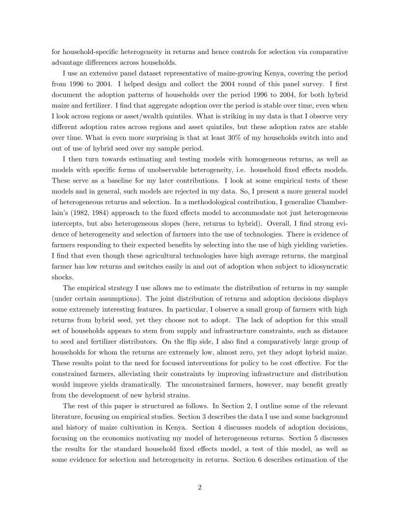
These two characteristics of hybrid maize are illustrated clearly in Figures 6a, 6b and 6c.

The �gures show the conditional distributions of yields across farmers who use hybrid and those

who do not for each of the three periods of data I use. It is clear from these �gures that the

mean of the hybrid yield distribution lies to the right of that of non-hybrid yields. The hybrid

yield distribution also has a lower variance than the non-hybrid yield distribution (the standard

14Also see Heckman and Honore (1990) and Borjas (1987).15The de�nitions and implications of absolute and comparative advantage as sorting mechanisms have been

outlined by various labor economists (see Willis (1986), Green (1991), Sattinger (1993) and Carneiro and Lee(2004)).

16One hypothesis for the lack of adoption and the persistence of non-hybrid maize is di¤ering tastes of hybridand non-hybrid maize, as in Latin America. This is unlikely in Kenya where the di¤erent maize varieties have auniform price and no distinction in the market.

9

deviations of the two distributions are signi�cantly di¤erent with p-values on the null of equal

standard deviations of 0.000 in each period). These �gures highlight an important property

of hybrid maize: it eliminates the lower tail of the distribution of outcomes under non-hybrid

maize. This is the main motivation for my model of heterogeneous returns. It is clear that the

farmers who would bene�t the most in terms of yields would be those at the lowest end of the

non-hybrid distribution of yields - the bad outcomes would be muted under hybrid.

The generalized Roy model allows for maximization of an underlying bene�t function that is

far more general than that in equation (8) so that hit = 1 if fH(yHit ; ZHit ) > fN (yNit ; Z

Nit ) where

Zjit represents sector j (j 2 H;N) costs and factors that a¤ect adoption, including the covariatesin the Xit�s. The simplest version of this bene�t function would be a pro�t maximization rule.

When output prices are the same for hybrid and non-hybrid maize, yields and pro�ts di¤er only

by (real) input costs. Throughout the empirical work, I will estimate yield functions, usually

controlling for complete input use. My data on inputs is not always at the crop level, but at the

�eld level so that calculating maize pro�ts directly is not as straight forward. The speci�cation I

use that estimates yield functions controlling for input use is close to estimating pro�t functions.

The more general version of a hybrid bene�t function for risk-neutral farmers allows for

unobserved costs and factors that are not in the yield equation to a¤ect the adoption decision.

These are the components of the Zit�s over and above the Xit�s that are in the yield equation.

Examples of variables that may be in this set of Zit�s that are not in the yield equation and are

not tastes include the distance from a household to the seed/fertilizer distributor and measures

of the availability of seed for a household in any period. Such measures of seed/input availability

clearly a¤ect the costs of planting hybrid maize (over and above the observed costs, which are

in the Xit�s) and can therefore a¤ect the adoption decision from period to period. In the case

of this generalized Roy model, any pattern of sorting is possible and the joint distribution

f(yH ; yN ) is required to understand the patterns of sorting and comparative advantage (the

standard program evaluation problem)17.

In particular, I can write the selection rule for a generalized Roy model for yields in terms

of a binary choice based on the latent variable, h�i , as

hit(yit) = 1 [h�it � 0] = 1

hZ0it� + u

sit � 0

i(9)

where hit is the binary adoption decision with respect to hybrid maize and h�it is the latent net

bene�ts of planting hybrid maize. usit is the selection error (the unobservable heterogeneity in

the adoption selection equation) and the Zit include not just the Xit�s from the yield equations,

but also the costs and other covariates that may a¤ect the adoption decision. The higher usitin equation (9), the more likely the farmer is to plant hybrid maize. Comparing this to the

strict Roy model (without costs) where the adoption decision was driven purely by di¤erences

in yields, h�it would just be yHit� yNit and u

sit would be u

Hit � uNit .

17The generalized Roy model still imposes the restriction that the selection rule can be expressed as a singleindex function. I consider the appropriateness of this restriction when I discuss my results.

10

Using a generalized yield function of the form

yit = hityHit + (1� hit)yNit (10)

I can substitute in equations (3) and (4) to get

yit = �Nt + (�Ht � �Nt )hit +X

0it

N +X0it(

H � N )hit + uNit + (uHit � uNit )hit (11)

Equation (11) illustrates the standard selection problem. If farmers know all or some part

of the errors uHit and uNit and act on what they know, then the decision to adopt hybrid, hit, will

generally be correlated with these errors (and hence with the composite error uNit +(uHit �uNit )hit

in equation (11)). The OLS estimate of �Ht ��Nt (and of the average treatment e¤ect) is thereforebiased, with the bias composed of both a selection bias and a sorting bias (see Heckman and Li

(2003)). For example, it may be the case that the farmers who plant hybrid may just have higher

soil quality land and/or better farm management (all of which are unobservable). Heterogeneity

of this �xed unobservables form has been emphasized in the literature, in particular with respect

to farm management (see Mundlak (1961)), productivity of farmers, and soil quality (see Conley

and Udry (2003) and Tittonell (2003)). In addition, there may even be heterogeneity in returns

to hybrid maize such that the farmers with the high returns to hybrid maize are the ones who

plant it. The average returns to hybrid maize computed by comparing farmers who plant hybrid

to those who do not are therefore overstated. My aim is to present a model that can account

for both these ideas.

In equation (11), the correlation of hit with (uHit � uNit ) is an issue. I will start with a

general decomposition of the uHit and uNit errors to allow for the possibility that the expected

gain to hybrid varies across farmers. The thought experiment is to consider a farmer i who

experiences low yields (say in the bottom quartile) when he plants non-hybrid maize. This can

be either permanent or transitory low yields - I will be more speci�c later. For this farmer i,

yNit < ct where ct is the percentile cut-o¤ to be in the bottom quartile of non-hybrid yields. His

percentage gain in yields is given by (assuming no Xit�s for simplicity) E�yHit � yNit j yNit < ct

�=

�Ht � �Nt + E�uHit � uNit j yNit < ct

�. Similarly, for a farmer who experiences high yields under

non-hybrid maize (in the upper quartile, say) so that yNit > kt, his expected gains will be

E�yHit � yNit j yNit > kt

�= �Ht � �Nt + E

�uHit � uNit j yNit > kt

�. I want a structure on the errors,

uHit and uNit , that allows these two expected gains to be di¤erent given the return to hybrid looks

higher for the farmers in the lowest quartile of the non-hybrid yield distribution.

I therefore consider the following factor structure on the errors18:

uHit = �Hi + �Hit (12)

uNit = �Ni + �Nit (13)

18This assumption is similar to the factor assumptions made in Carneiro, Hansen and Heckman (2003), exceptthat I exploit the panel nature of the problem and assume the correlated factors are time-invariant.

11

The �Hit and �Nit are assumed to be uncorrelated with each other, as well as with the Xit�s and

Zit�s, unlike the �Hi and �Ni . This assumption amounts to the transitory errors �Hit and �

Nit not

being allowed to a¤ect the farmer�s decision to use hybrid, though the �Hi and �Ni will. The

timing of the production of maize and the fact that it is all rain fed is important here. Farmers

are assumed to know their �Hi and �Ni , but not the �Hit and �

Nit . The seed type (hybrid or non-

hybrid) is usually �xed before the �it shock is realized. Most farmers plant right before the onset

of rains or at the onset of rains (though this is late), but the extent of the rains is unknown.

Inputs such as labor and fertilizer may be correlated with the shock, for example rainfall, but

the key is that I observe rainfall. So, conditional on the covariates a¤ecting yields I have in my

data (most importantly, seasonal rainfall), the assumptions underlying the �Hit and �Nit are more

defendable.

The above structure on the errors allows for maize variety speci�c unobservables, �Hi and

�Ni , to a¤ect yields under hybrid and non-hybrid maize respectively. However, it is only possible

to identify a relative relationship between the �Hi and �Ni unobservables. It is this relative

relationship that leads to the idea of comparative advantage in technology adoption and what

role this comparative advantage plays, if any, in returns to hybrid technologies.

Substituting the factor structure on the errors into the yield equations in (3) and (4), I get

yHit = �Ht + �Hi +Xit

H + �Hit (14)

yNit = �Nt + �Ni +Xit

N + �Nit (15)

Following Heckman and Honore (1991), Lemieux (1998) and others, I use the linear projections

of the �Hi and the �Ni on (�

Hi � �Ni ) as follows

�Hi = bH(�Hi � �Ni ) + � i (16)

�Ni = bN (�Hi � �Ni ) + � i (17)

where, by construction, the projection coe¢ cients are bH = (�2H � �HN )=(�2H + �2N � 2�HN ),

bN = (�HN � �2N )=(�2H + �2N � 2�HN ) and �HN � cov(�Hi ; �

Ni ), �

2H � V ar(�Hi ), and �

2N �

V ar(�Ni )19. I de�ne the � i to be the absolute advantage as its e¤ect on yields does not vary

by the choice of hybrid/non-hybrid. I de�ne �Hi � �Ni to be the comparative advantage gain

from growing hybrid, which is orthogonal to the absolute advantage by construction. I can then

re-de�ne this comparative advantage gain to be �i as follows:

�i � bN (�Hi � �Ni ) (18)

This is just a rede�nition of the sector speci�c unobservables �Hi and �Ni . The �i serves as a

19The � i�s in equations (16) and (17) are the same. Subtracting equation (17) from equation (16) implies that�Hi � �Ni = (bH � bN )(�Hi � �Ni ). For the � i�s to be equal across sectors, bH � bN must be equal to 1, which is

easily shown: bH � bN = �2H��HN��HN+�2N

�2H+�2

N�2�HN

= 1:

12

measure of comparative advantage in my model. Recall that it is possible to identify only the

relative e¤ect of �i in the hybrid sector, see Carneiro, Hansen and Heckman (2003). Allowing

� bH=bN ; equations (16) and (17) become

�Hi = �i + � i (19)

�Ni = �i + � i (20)

Substituting these back into equations (14) and (15),

yHit = �Ht + � i + �i +Xit H + �Hit (21)

yNit = �Nt + � i + �i +Xit N + �Nit (22)

The expected gain for a farmer from using hybrid is now a function of both observed and

unobserved household characteristics:

Bit = yHit � yHit = (�Ht � �Nt ) + ( � 1)�i +X 0it(

H � N ) (23)

These descriptions of the logarithmic production functions for the case of heterogeneous

returns map back into a generalized version of the Cobb-Douglas production functions I started

with so that Y Hit = e� ie� i e�

Ht

kQj=1

X Hjijt

!e�Hit and similarly for Y Ni except without the e�

i term.

The motivation for this structure of production functions comes from the fact that hybrid maize

increases mean yields and reduces the variance in yields. We would expect individuals who are

in the lower tail of the non-hybrid distribution (who have bad outcomes) to bene�t the most

from the use of hybrid maize. The production functions illustrate these properties directly:

when < 1, farmers with �i < 0 will have high rewards from hybrid maize (and low rewards

if > 1), while farmers with �i > 0 will have lower rewards from hybrid maize (vice versa if

> 1).

I can substitute equations (19) through (22) into the generalized yield equation (10) to derive

yit = �Nt + �i + (�Ht � �Nt )hit +X 0

it N + ��ihit +X

0it(

H � N )hit + "it (24)

where � � ( �1) is the coe¢ cient on the household speci�c comparative advantage component�i and �i � �i + � i. "it is assumed to be the unanticipated component of yields where "it =

�Nit + (�Hit � �Nit )hit. The coe¢ cient on hit, ��i, depends on the unobserved household-speci�c

e¤ect �i, implying a random coe¢ cient model.

The coe¢ cient on hit, ��i, is correlated with decisions to adopt (i.e. hit itself). Thinking

in terms of the generalized Roy model framework, the household-speci�c expected gain Bit is

allowed to enter the latent index determining sector choice, hit. Hence, the coe¢ cient ��i is

generally correlated with the dummy variable hit if agents use their expected gains from growing

hybrid in deciding whether or not to plant hybrid. This framework implies a correlated random

13

coe¢ cient (CRC) model, which I show in the empirical work is a generalization of Chamberlain�s

(1984) correlated random e¤ects (CRE) model where household-speci�c intercepts are allowed

to be correlated with hit. The CRC model allows both the household-speci�c intercepts as well

as household-speci�c slopes/returns to be correlated with hit. As I discuss in detail, this model

can be estimated via methods similar to those introduced by Chamberlain (1984).

�i and � i are uncorrelated by construction, and since the household-speci�c slope is ��i, the

covariance between individual speci�c slopes and intercepts in the yield function is:

cov(�i; ��i) = ��2� (25)

The structural coe¢ cient � therefore determines whether high intercept households also have

the higher returns to hybrid maize. If � > 0, then > 1, and the use of hybrid in�ates the

role of comparative advantage in the hybrid sector. In the long run, this would lead to greater

inequality in yields in the overall economy.

Equation (24) is a generalization of the household �xed e¤ects model. To illustrate this, let

= 1 so that there is now the same �xed unobservable heterogeneity (for example, due to farm

management, farmer productivity or soil quality) that a¤ects yields irrespective of the type of

maize seed planted. This imposes very speci�c assumptions on the error structure, in particular

that uHit = �i + �Hit and uNit = �i + �Nit and that the di¤erence (�

Hit � �Nit ) must be independent

of the selection rule. This implies that the timing of the decision to use hybrid maize at any

point in time is independent of the yield di¤erence facing a farmer at that time.

The yield function corresponding to this error structure is the �xed e¤ects version of equation

(24):

yit = �Nt + �i + (�Ht � �Nt )hit +X 0

it N +X 0

it( H � N )hit + "it (26)

where "it = �Nit + (�Hit � �Nit )hit. The expected gain to growing hybrid is therefore:

Bit = (�Ht � �Nt ) +X 0

it( H � N ) (27)

In this �xed e¤ects model, the expected gain from hybrid in equation (27) can vary across

households as long as it is a function of the observable Xit�s. But, the unobservable heterogeneity

or �xed e¤ect �i is restricted to a¤ect yields identically whether or not a farmer uses hybrid.

The �xed e¤ect therefore does not appear in equation (27). The �xed e¤ects yield function

can be estimated from two periods of panel data on the same farmers under the assumption

that, conditional on the �i, the error in the yield function is uncorrelated with the decision

to adopt hybrid maize. This requires that the source of heterogeneity driving the endogeneity

must manifest itself in an �i that is �xed across households and that does not vary by the

hybrid/non-hybrid choice.

The main contribution of this paper is to relax the assumption that the return to hybrid maize

varies by only observable dimensions across households. I draw on recent empirical studies in

labor economics that allow for generalizations to the �xed e¤ects model, and use the framework

14

described above that allows for comparative advantage in the adoption decision. Advances in

techniques have been made in the context of experimental data (for example, Heckman, Smith

and Clements (1997)) and in cross sectional data where the covariate of interest is a stock

variable like schooling. I use the panel nature of my data and build upon the approaches of

Lemieux (1993, 1998) and Card (1996)20. To estimate the model in equation (24), I generalize

the multivariate regression/minimum distance approach of Chamberlain (1984) to allow for

heterogeneous coe¢ cients.

5 Baseline Results

I begin the empirical work by looking at the OLS and household �xed e¤ects speci�cations as

a baseline to the heterogeneous returns model. Table 3 shows these OLS and household �xed

e¤ects results for speci�cations with and without covariates. The OLS and household �xed

e¤ects results reported here are for a simpli�ed version of equation (26):

yit = � + �hit +X0it + �i + uit (28)

Comparing this to equation (26), allowing �Ht � �Nt � �t, I have assumed that �t = � 8t. Inaddition, I have assumed that H = N = . I will relax the latter of these assumptions in later

results. The former can be relaxed but relaxing it is empirically unimportant - the results from

the more complicated model that allows for time-varying ��s are similar so I report results for

the simpler model throughout.

The OLS estimates in the �rst column of Table 3 are extremely large and positive: households

that plant hybrid maize tend to have much higher maize yields, on the order of 100% higher.

Also note the strong time trends in yields for my sample of households over this period. Adding

province dummies in the second column of Table 3 decreases the coe¢ cient on hybrid, as there

are strong di¤erences across provinces in both yields and hybrid use. In the third column, I add

covariates to the speci�cation. The purpose of these covariates is to control for other household

variables that could a¤ect yields, and that may be correlated with the use of hybrid maize,

mostly inputs. They include land acreage, fertilizer (results are robust to whether quantities or

total expenditure are used), land preparation costs, seed quantity, variables that measure labor

inputs (both hired and family labor where possible), long term mean seasonal rainfall, current

seasonal rainfall, year dummies and province dummies. Adding these covariates decreases the

OLS coe¢ cient further, though it is still quite large at 56%. The fourth and �fth columns of Table

3 report the household �xed e¤ects results. The coe¢ cient on hybrid decreases dramatically,

though with covariates the di¤erence between the OLS and �xed e¤ects is less substantial.

There is still a substantial return to hybrid maize even within households, controlling for �xed

unobservable heterogeneity and a wide set of covariates, on the order of 15%.

20Some of these issues have been debated in the literature on the return to unionization, see Vella and Verbeek(1998), Green (1991) and Robinson (1989) for examples.

15

This household �xed e¤ects framework is restrictive in the assumptions it imposes on the

adoption process and the comparison of the adopters and non-adopters. A consequence of the

restrictions it imposes is that there is assumed to be no di¤erence between farmers who switch

into the use of hybrid and those that switch out of the use of hybrid. The �i allows some

farmers to be more productive overall (higher �i), but the di¤erence across the hybrid and non-

hybrid sectors is the same for all farmers, irrespective of their transition histories. Apart from

the permanent component in the outcome equation, �i, the adoption decision cannot depend

on observed outcomes except under restrictive assumptions on the transitory component (see

Ashenfelter and Card (1985)). Such assumptions can be motivated by myopia or ignorance of the

potential gains from planting hybrid, but they are unrealistic here21. In addition, as emphasized

by Card (1998), the �xed e¤ects model requires that the selection bias for a given characteristic,

such as farmer experience or soil quality, must be of the same sign for all individuals. It does

not allow, for example, selection into hybrid to be positive for people with low education, say,

but negative for those with high education.

For various agronomic and economic factors, such as the slow spread of information and the

credit constraints that are alluded to in the literature, it is reasonable to allow for a distribution

of returns to the technology that relies on both observed and unobserved factors. The household

�xed e¤ects model may therefore not be appropriate for the question at hand. The rest of this

section describes tests of the household �xed e¤ects model, and some intuitive evidence for

selection and heterogeneity in returns.

5.1 Two Period CRE Model

The household �xed e¤ects estimates are consistent only under the assumption of strict exo-

geneity of the errors. Chamberlain�s CRE approach provides a basis for testing this assumption

(see Chamberlain (1984) and Jakubson (1991)). I illustrate the simple two period, no covariates

CRE model, for which the data generating process is given by

yit = � + �hit + �i + uit (29)

The assumption of strict exogeneity of the errors is:

E(uitjhi1; :::; hiT ; �i) = 0 (30)

CRE illustrates how the �xed e¤ects model is overidenti�ed. Replace the �xed e¤ect, �i, by its

linear predictor based on the history of the covariates:

�i = �0 + �1hi1 + �2hi2 + vi (31)

21Hybrid maize was introduced in the 1960�s, with widespread use of extension services to promote the tech-nology. See Evenson and Mwabu (1998).

16

where the projection error vi is uncorrelated with hi1 and hi2 by construction, and the ��s are

the projection coe¢ cients. Substituting this linear projection into the yield equation,

yit = � + �hit + �0 + �1hi1 + �2hi2 + vi + uit (32)

Let �it = vi + uit where E [�ithi1] = E [�ithi2] = 0. For each time period, therefore:

yi1 = (� + �0) + (� + �1)hi1 + �2hi2 + �i1 (33)

yi2 = (� + �0) + �1hi1 + (� + �2)hi2 + �i2 (34)

These are the structural yield equations for each period. I estimate reduced form yield functions

for each period of the form

yi1 = �1 + 1hi1 + 2hi2 + �i1 (35)

yi2 = �2 + 3hi1 + 4hi2 + �i2 (36)

Equations (33) through (36) show how the �xed e¤ects model is overidenti�ed. From the

four reduced form coe¢ cients, 1; 2; 3 and 4, I can estimate the three structural parameters,

�1; �2 and � using minimum distance. It is important to note that estimating the CRE model

does not require a speci�cation of the conditional expectation of the �i. Neither does it require

knowledge of the true conditional expectation of the �i.

The intuition behind the identi�cation of the CRE model comes from the underlying as-

sumption of the strict exogeneity of the errors. If the �xed e¤ects model is valid, then the only

way the history of hit (both past and future) a¤ects the current outcome is through the house-

hold level unobservable, �i. The identi�cation of � comes from those individuals who switch

hybrid status hit during the course of the panel. Conditional on �i and the included regressors,

the switching behavior is taken to be exogenous and driven by transitory factors uncorrelated

with the rest of the model. This is testable with panel data as described above. The structural

estimates are overidenti�ed even in the two period case. The minimum distance estimator of the

structural parameters is also the minimum �2 estimator if the weight matrix used is the inverse

of the variance covariance matrix of the reduced form coe¢ cients. This is called the optimal

minimum distance (OMD) estimator. If the identity matrix is used as the weight matrix in-

stead, the estimates are referred to as equally weighted minimum distance (EWMD) estimates.

The OMD estimates are e¢ cient, but they can be biased in small samples and can therefore

be out-performed by EWMD (see Altonji and Segal (1996)). Throughout, I report both sets

of estimates, as well as the �2 statistics on the OMD problem, which are just the value of the

minimand in the OMD problem.

Estimates of the CRE model for three periods, both with and without covariates are shown

in Table 4. In the CRE model, covariates can be treated as either exogenous or endogenous.

Exogenous covariates enter the model in equation (29), but are assumed to be uncorrelated

with the �xed e¤ect so that they do not enter the projection in equation (39). Endogenous

17

covariates, on the other hand, are correlated with the �xed e¤ect and enter the projection.

The CRE model therefore allows tests of whether covariates are endogenous. I report estimates

where all covariates (other than the choice to plant hybrid) are assumed to be exogenous, though

allowing for endogenous covariates does not change the results.

Table 4 shows both the reduced form and structural estimates for various speci�cations. The

reduced forms in the upper panel of Table 4 give nine reduced form parameters (not including

the constants or covariates), from which I use minimum distance to estimate the four structural

estimates, shown in the lower panel of the table. Three of these structural estimates are the

��s from the linear projection of the �xed e¤ects and the fourth is the estimate of the return

to hybrid, �. The CRE estimates of � in all cases are very close to the household �xed e¤ects

estimates in Table 3, as expected. The OMD and EWMD estimates of � are quite similar, all

within sampling error of each other. The last column in the lower panel of Table 4 shows the

�2 values on the overidenti�cation test. In all cases, I can reject the null that the minimum

distance restrictions hold. This overidenti�cation test is an omnibus test. It has low power

against any speci�c alternative, but it does have power against many alternatives. It is therefore

not surprising that I am able to reject the overidentifying restrictions.

5.2 Preliminary Evidence of Heterogeneity

To motivate my framework of heterogeneous returns, I report some tests for heterogeneity (see

Heckman, Smith and Clements (1997)). These are purely for illustrative purposes, as they ignore

the role of selection and assume that the data is experimental, i.e. that farmers using hybrid

and non-hybrid maize are the same on average. This is an extremely strong assumption. Let the

conditional yield distributions for the adopters and non-adopters of hybrid be FH(yH jh = 1)

and FN (yN jh = 0) respectively (shown in Figures 6a, 6b and 6c). The conditional distributionsallow us to bound the unknown joint distribution of interest, F (yH ; yN jh = 1), via the Frechet-Hoe¤ding bounds22 which also bound the variance, V ar(yH � yN ). A test of whether the lowerbound of V ar(�y) is signi�cantly di¤erent from zero is a test for heterogeneity in returns. I

can look at whether each percentile of the hybrid and non-hybrid yield distributions di¤ers by

a common constant with the null hypothesis H0 : q(yH) � q(yN ) = k for all q such that 0 �q � 10023. Figures 7a, 7b and 7c show the di¤erences in percentiles of the returns distributions,assuming perfect positive dependence, and Figures 8a and 8b show similar plots for my samples

of joiners (farmers who do not use hybrid one period but do the next) and leavers (vice-versa).

Appendix Table A2 shows the full set of results where I can reject the null hypothesis above.

22The Frechet-Hoe¤ding bounds are given by:max

�FH(yH jh = 1) + FN (yN jh = 1)� 1; 0

�� F (yH ; yN jh = 1) � min[FH(yH jh = 1); FN (yN jh = 1)]

23 I need to make assumptions about the dependence in the hybrid and non-hybrid conditional yield distrib-utions. The two extreme dependence assumptions are perfect positive dependence (the individual at the 99thpercentile in the hybrid distribution would be at the 99th percentile of the non-hybrid distribution had he notplanted hybrid) and perfect negative dependence, where the percentile rankings are assumed to be reversed.

18

5.3 Evidence of Selection

Assuming away selection is hardly tenable; in Table 5, I look for evidence of selection. I split the

adoption history into dummies describing the transitions of households across technologies over

the three periods. The idea is to look at whether households with di¤erent transition histories

have di¤erent returns in terms of yields to planting hybrid (see Card and Sullivan (1988)). To

understand transition histories, I de�ne a �joiner� to be a farmer who does not plant hybrid

the �rst period, but does the next, and a �leaver�to be a farmer who plants hybrid one period,

but not the next. Similarly, I de�ne a �hybrid stayer�to be a farmer who plants hybrid in both

periods and a �non-hybrid stayer� to be one who plants traditional varieties in both periods.

Under a household �xed e¤ects model, the selection is re�ected by the coe¢ cients on the stayers

and leavers in the periods in which they are not growing hybrid.

I look at each pair of periods in my data and compare yields for the hybrid and non-hybrid

stayers, the joiners, and the leavers in each of the two periods separately to learn about the

extent of selection. For example, the �rst two columns in Table 5 look at the transitions of

households over 1997-2000, with the omitted group being the non-hybrid stayers. The �rst and

second columns of this table compare the yields in 1997 and 2000 for hybrid stayers, joiners and

leavers in 1997 and 2000 separately. If there was no selection at all (not even via a household

�xed e¤ect), we would expect the coe¢ cient on the leavers in the yield equation for 1997 to

be no di¤erent from the coe¢ cient on the stayers, and also no di¤erent from the coe¢ cient

on the joiners in the yield equation for 2000. Similarly, the coe¢ cient on joiners in the yield

equation for 1997 would be no di¤erent from zero, as should the coe¢ cient on the leavers in the

yield equation for 2000. Hence, the coe¢ cient on the leavers and joiners across the two yield

equations illustrates the extent of selection. Table 5 reports similar estimates for 2000-2004 and

1997-2004. The hybrid stayers uniformly get the largest yields and the leavers and joiners get

very di¤erent changes in yields when they switch their adoption status.

In Table 6, I look for heterogeneity in returns to hybrid seed along observable dimensions.

This relaxes the assumption that H = N = in the OLS and FE estimations reported

above. Table 6 reports results for yield functions estimated separately for hybrid and non-

hybrid households. I report both the OLS as well as household �xed e¤ects speci�cations. The

returns to observables di¤er by the use of hybrid, especially in the cases of fertilizer and rainfall.

This holds for both the OLS as well as the household �xed e¤ects speci�cations. The last row

of Table 6 reports estimates of the return to hybrid (evaluated at the mean Xit�s) for the case

where the returns to observables are allowed to vary across hybrid and non-hybrid use. There

is a signi�cant return to hybrid for both the OLS and �xed e¤ects speci�cations, even after

allowing for returns to vary by the observables.

19

6 Estimating a Model with Heterogeneous Returns

The model of heterogeneous returns outlined earlier implies the following econometric model in

maize yields for the simple two period, no covariates case:

yit = � + �hit + �i + ��ihit + �it (37)

For simplicity, I focus only on hybrid maize and leave out other inputs to explain the empir-

ical strategy and then discuss extensions. The model above24 can be estimated as per Lemieux

(1998), using non-linear 2SLS. Instead, I extend the basic Chamberlain CRE approach to a

scenario of correlated random coe¢ cients. This may be somewhat easier and allows a �2 overi-

denti�cation test, similar to that described above. The next sections are devoted to describing

my estimation and identi�cation strategy, keeping in mind the intuition of the CRE approach.

I then describe extensions to this basic model and the estimation results.

6.1 Two Period CRC Model

For the simple two period, no covariates case, the yield function is given by equation (37)

above. The key identifying assumption here is that, conditional on the comparative advantage

component ��ihit (and the covariates in the more general speci�cations), the unanticipated

component of yields, "it, is not correlated with the decision to adopt. Remembering that �i ��i + � i, where �i and � i are orthogonal, I re-write equation (37) as

yit = � + �i + �hit + ��ihit + � i + "it (38)

Using the same idea as CRE, I linearly project the �i�s onto the history of the hybrid decisions,

as well as their interactions so that the projection error is orthogonal to hi1 and hi2 individually

as well as to their product, hi1hi2 by construction25. The projection is given by

�i = �0 + �1hi1 + �2hi2 + �3hi1hi2 + vi (39)

24This empirical model is similar to models of individual speci�c heterogeneity in Heckman and Vytlacil (1997),Card (2000, 1998), Deschênes (2001), Carneiro, Hansen and Heckman (2001), Carneiro and Heckman (2002), andWooldridge (1997). Lemieux (1998) has a very similar model to look at whether the return (in terms of wages)to both observables and unobservables varies by union sector membership.

25The projection I use here is di¤erent from what CRE uses. If I use the simple CRE projection, �i =�1hi1 + �2hi2 + vi, and substitute this into the yield function,

yit = �0 + �1hi1 + �2hi2 + �hit + ��0 + ��1hi1hit + ��2hi2hit + vi + �vihit + uit

Even though vi, the projection error, is linearly uncorrelated with hi1 and hi2 individually, it is generally correlatedwith their product, hi1hi2, so that E [vihi1hi2] 6= 0. The projection I use must therefore include the interactionsof the hybrid histories.

20

In addition, I normalize the �i�s so thatP�i = 0. Since hit is a dummy variable, substituting

the above projection into the yield equations gives:

yit = �+�0+�1hi1+�2hi2+�3hi1hi2+�hit+��0hit+��1hi1hit+��2hi2hit+��3hi1hi2hit+vi+�vihit+uit

(40)

For each of the two time periods, the yield functions are:

yi1 = (�+�0)+[�1(1+�)+�+��0]hi1+�2hi2+[�3(1+�)+��2]hi1hi2+(vi+�vihi1+ui1) (41)

yi2 = (�+�0)+�1hi1+[�2(1+�)+�+��0]hi2+[�3(1+�)+��1]hi1hi2+(vi+�vihi2+ui2) (42)

The corresponding reduced forms are:

yi1 = �1 + 1hi1 + 2hi2 + 3hi1hi2 + �i1 (43)

yi2 = �2 + 4hi1 + 5hi2 + 6hi1hi2 + �i2 (44)

Equations (43) and (44) give six reduced forms coe¢ cients ( 1; 2; 3; 4; 5 and 6), from

which I can estimate the �ve structural parameters (�1; �2; �3; � and �) using minimum dis-

tance26. The structural parameters are clearly overidenti�ed and the restrictions for the mini-

mum distance problem are:

1 = (1 + �)�1 + � + ��0

2 = �2

3 = (1 + �)�3 + ��2

4 = �1

5 = (1 + �)�2 + � + ��0

6 = (1 + �)�3 + ��1 (45)

I now discuss extensions to this basic model and whether the �i�s themselves can be recovered

from this estimation.

6.2 Extensions

I consider the following extensions:

1. Covariates: all the identi�cation arguments presented above generalize when the model

includes covariates. Covariates in the CRE model can be thought of as either exogenous or

endogenous, the latter implying that they are correlated with the �xed e¤ects. Allowing for

26There may seem to be six structural parameters, given the presence of �0 in equations (39) and (45). However,given the normalization that

P�i = 0, then �0 is just a function of the hybrid histories, their interactions and

the other �0s. In particular, �0 = ��1hi1 � �2hi2 � �3hi1hi2 where hi1 and hi2 are the averages of the adoptiondecisions of households in periods one and two, and hi1hi2 is the average of the interaction.

21

endogenous covariates in CRE is straight forward: all the leads and lags of the endogenous

covariates are included in the projection. The CRC model is slightly more complicated and

can become cumbersome. Endogenous covariates are de�ned similarly - they are correlated

with the �i�s. I allow for fertilizer to be an additional endogenous covariate so that the

CRC projection generalizes to

�i = �0 + �1hi1 + �2hi2 + �3hi1hi2 + �4hi1fi1 + �5hi2fi1 + �6hi1hi2fi1

+�7hi1fi2 + �8hi2fi2 + �9hi1hi2fi2 + �10fi1 + �11fi2 + vi (46)

where fit for t = 1; 2 represents the use of fertilizer in each period. The other covariates

enter the problem in such a way that they are exogenous (uncorrelated with the �i�s)27.

2. Three periods: this is a simple extension. For space considerations, I do not show the

restrictions for the three period model. The problem becomes heavily overidenti�ed with

only 9 structural parameters to estimate from the 21 reduced form coe¢ cients for the

base case with no other endogenous covariates. However, as covariates are allowed to be

endogenous, the model becomes cumbersome.

3. Joint choice variables: the two-sector model presented above (hybrid/non-hybrid) can

be extended to multiple sectors. An additional technology use sector, like fertilizer, can

be incorporated by thinking of a four sector model (farmers use either both hybrid and

fertilizer, neither, one or the other). I simplify it further. In 1997, for example, 76% of

households �t into one of two of the possible four sectors, namely using both hybrid maize

and fertilizer or neither. So, I estimate an easier model that rede�nes sectors to this joint

decision (using both hybrid and fertilizer or not) and looks at the heterogeneity in returns

across these two sectors.

6.3 CRC Estimates

This section describes various estimates of the CRC model. I report estimates for the pure

hybrid model described in detail above (with and without covariates) for both the two and three

period cases. In addition, I report results for the endogenous covariate and joint hybrid-fertilizer

extensions to the basic model that I described in the previous section. Recall that a covariate

is described as endogenous if it is assumed to be correlated with the �i�s and therefore enters

the projection in equations (39) or (46) (similarly, a covariate is exogenous if it is assumed to

be uncorrelated with the �i�s).

Tables 7, 8a, 8b and 9 present the CRC model reduced form and structural estimates. These

tables report both the EWMD and OMD estimates for cases with and without covariates, as

27There is some justi�cation for this. Using the estimates from the pure hybrid problem in Tables 7 and 8, Iam able to look at the distribution of predicted �i�s and correlate this with the covariates. Of all the covariates,only the correlations between the �i�s and fertilizer are important in magnitude and signi�cance.

22

well as the �2 statistics on the overidenti�cation tests for the OMD cases. The coe¢ cient of

interest is �, i.e. the coe¢ cient on the individual speci�c comparative advantage components,

�i. Table 7 presents the two period reduced forms for the CRC model, both with and without

covariates, using data for 1997 and 2004. These are the reduced form estimates for the most basic

speci�cation described above where hybrid is the only endogenous variable and the projection

used is given by equation (39). Table 8a reports the structural estimates for this speci�cation:

the OMD and EWMD results, along with the �2 statistics, all with and without covariates. The

estimates of � are consistently negative, though with quite large standard errors in the EWMD

cases.

Table 8b presents two sets of structural estimates of � that account for fertilizer possibly

entering the household�s decision making process regarding hybrid maize instead of restricting it

to be exogenous. I do this in two ways. In the upper panel of Table 8b, I allow for the fertilizer

covariate to be endogenous in the sense of being correlated with the �i�s, as in equation (46).

Again, the estimates of � in this panel of Table 8b are consistently negative, both with and

without covariates as well as across OMD and EWMD. The lower panel in Table 8b reports

results for the case where there is a joint hybrid-fertilizer decision on the part of the farmer

so that he is in the so called technology sector if he uses both hybrid maize and fertilizer,

otherwise he is not. This is similar to the original hybrid model, except the dummy variable for

technology is no longer a dummy variable for the use of hybrid maize, but instead it is a dummy

variable for whether the farmer is in the technology sector or not. The reason for estimating

this model is that in the three period case allowing fertilizer to be directly correlated with the

�i�s as in equation (46) makes the model too cumbersome. Hence, I settle for a simpler model

and account for the endogeneity of fertilizer use by describing the joint hybrid-fertilizer decision.

I also estimate this model for the two periods case to have comparable results. The results in

Table 8b for two periods are consistent with the previous estimates reported for �.

Table 9 shows the structural estimates (the reduced forms are available upon request) for

the three period CRC models for two cases: pure hybrid decision and the joint hybrid-fertilizer

decision. Recall that there are three reduced forms here, one for each period, that contain all

the possible interactions of the three hybrid histories. This implies a total of 21 reduced form

estimates that can be mapped onto the 9 structural estimates: 7 ��s from the projection of the

�i�s, the average return to hybrid, �, and the comparative advantage coe¢ cient, �. These results

are shown in Table 9; all the the estimates reported allow for the full set of exogenous covariates

(acreage, real fertilizer expenditure, land preparation costs, seed, labor variables and rainfall

variables). The estimate of � varies across the speci�cations, though the OMD estimates are

consistently negative. For the joint fertilizer-hybrid problem, both the OMD and EWMD are

negative and signi�cant.

23

6.4 Recovering the Distribution of b�iBefore I move on to the conceptual discussion of my model and estimates, I look brie�y at

the distribution of the predicted �i�s. Given the CRC structural estimates of the ��s and the

form of the projection given by either equations (39) or (46), I can predict the �i�s for a given

history of hybrid use. However, I must assume that the projections describe the true conditional

expectation of the �i�s. This is essentially an assumption only for the case of equation (46) as

in the case of equation (39) since hit is binary and each history is accounted for, the projection

is saturated. Once I have the predicted distribution of comparative advantage, �i, I can derive

the distribution of the predicted � i�s via the yield function.

Figure 9a shows the distribution of the predicted �i�s in my sample for the two period model

with the full set of exogenous covariates (the estimates come from the last column in Table 8a).

Since the predicted �i�s are obtained from the projection in equation (39), the distribution of the

predicted �i�s is just four mass points: think of these as averages of the individual underlying

�i�s for each history and interaction of histories of hybrid use. There are only four possible

hybrid histories: hybrid stayers, non-hybrid stayers, leavers and joiners. Hence, there are only

four possible values of b�i : 0:069;�0:369; 0:227 and 0:403 for the four histories respectively. Thenon-hybrid stayers have the negative (and lowest) predicted �i�s and hence the highest returns

to hybrid, since � < 0. Meanwhile the joiners and leavers have the lowest returns (indicating

they are the more marginal farmers) and the hybrid stayers have almost zero returns. Figure 9a

shows these four mass points in the b�i distribution by farmers hybrid use status in 1997. Themass point at the extreme left corresponds to the non-hybrid stayers, the next (moving from

left to right) are the hybrid stayers, followed by the leavers and then the joiners.

Figure 9b shows the distribution of the b�i�s for the case where both hybrid maize and fertilizeruse are endogenous (the estimates come from the last column in the upper panel of Table 8b).

Here, the distribution of the predicted b�i�s is continuous since the predicted b�i�s come from the

projection in equation (46). Again, Figure 9b splits out the distribution by hybrid use in 1997.

From Figure 9b it is not clear where the four di¤erent types of farmers lie in this distribution,

but I can look at the mean of the predicted b�i�s for each hybrid transition history. I �nd thatthe mean b�i for the non-hybrid stayers is the lowest at �0:236, the hybrid stayers are next at�0:015, followed by the leavers (0:253) and then the joiners (0:437). Finally, Figure 9c showsthe corresponding distribution of the predicted � i�s (which were constructed to be orthogonal

to hybrid choice) for 1997 adopters and non-adopters.

7 Robustness Checks

This section presents some robustness checks. As the �rst robustness check, I look at the stan-

dard control function and treatment e¤ect estimates of the yield returns to hybrid maize. This is

a broad set of approaches that includes the familiar Heckman two-step estimator, more general

control function estimators (see Garen (1984) and Deschênes (2001)), as well as a description of

24

treatment e¤ects under non-random assignment, i.e. the ATE, TT, MTE and LATE (see Björk-

lund and Mo¢ tt (1987), Heckman (2001), Heckman, Tobias and Vytlacil (2001) and Carneiro

and Heckman (2002)).

I rewrite equation (11) for one time period,

yi =�� +X

0i(

H � N ) + (uHi � uNi )�hi +X

0i N + uNi � �ihi +X

0i N + uNi (47)

Estimates of �i would illustrate whether the average returns of farmers selecting into using

hybrid maize are higher than the returns for the farmers at the margin. The reverse is possible

such that the marginal return is greater than the average when costs are su¢ ciently positively

correlated with returns (i.e. the farmers with high returns are the farmers that also face high

costs). With assumptions of normality on this model, it is possible to estimate the standard

cross sectional selection parameters. However, these selection correction procedures are cross

sectional in nature and impose distributional assumptions. They do not fully address the issues

I am interested in, nor do they fully exploit the panel nature of my data.

The yields in the hybrid and non-hybrid sectors are given by equations (3) and (4), and the

selection equation is given by equation (9). Drawing on Heckman, Tobias and Vytlacil (2001),

I look at the following treatment e¤ects:

ATE(x) = E(�jX = x) = x( H � N ) (48)

TT (x; z; h(Z) = 1) = x( H � N ) + (�H�H � �N�N )�(z�)

�(z�)(49)

MTE(x; us) = x( H � N ) + (�H�H � �N�N )us (50)

where � = yH�yN is the yield gain from hybrid, �H�H and �N�N correspond to the coe¢ cienton the selection term in a two-step selection model. I assume V ar(us) = 1 so that �2H =

V ar(uHi ), �2N = V ar(uNi ), �H = Corr(uHi ; u

si ) and �N = Corr(uNi ; u

si ). �(:) and �(:) represent

the normal probability and cumulative distribution functions respectively where �(z�)�(z�) is the

Inverse Mills ratio/selection correction term for the hybrid yield function (a similar selection

term is computed for the non-hybrid yields).

These treatment e¤ects in the case of joint normality are simple to compute. They involve

a two-step control function procedure: I �rst run a probit of selection and control for estimates

of the selection (Inverse Mills ratio) terms in the second step that looks at sector speci�c yield

functions. The ATE uses the estimates of the coe¢ cients on the Xi�s from this second step. The

TT adjusts this estimated ATE for the selection into planting hybrid. The MTE looks at the

treatment e¤ect as a function of the unobservables in the selection equation: it describes whether

people who are more likely to use hybrid for unobservables reasons (the usi ) have higher or lower

returns from planting hybrid. If the coe¢ cient on us in equation (50) is negative, it implies

that farmers with unobservables that make them the least likely to use hybrid have the highest

yield return to planting hybrid. The MTE is needed to understand whether heterogeneity is

25

important and the role of unobservables that make farmers more or less likely to use hybrid.

These treatment e¤ects are shown in Table 10 for every cross-section of my data. I need an

exclusion restriction (or instrument), i.e. a variable that enters the selection equation (9), but not

the yield functions in (3) and (4). I use a variable that describes a household�s access to fertilizer

and hybrid seed. The survey question that households are asked is what the distance between

their homestead and the closest stockist of fertilizer is (not the distance to where fertilizer

is actually purchased). This distance measure gives an idea of the access and availability of

the technologies. The results are similar if I use the interaction of the same distance variable

with asset quantiles as the exclusion restrictions, while allowing the main e¤ects of both asset

quantiles and distance to enter the yield equations.

The ATE�s (evaluated at the mean of the Xi�s) are all extremely large and positive, ranging

from 0.756 in 2000 to 2.097 in 1997. The TT estimates are consistently smaller, ranging from

0.677 to 1.374. The MTE slope, meanwhile, is consistently negative across all three samples:

�1.769 (with a standard error of 0.775) in 1997, -0.222 (0.370) in 2000 and -0.911 (0.251) in

2004. In two of these cases, the slope of the MTE function with respect to us is negative and

signi�cantly di¤erent from zero. This implies that farmers with unobservables that make them

most likely to use hybrid get the lowest returns from hybrid. In addition, I can estimate the

instrumental variable (i.e. the LATE) estimate using the same exclusion restriction. The IV

estimates of the return to hybrid, reported in the lower panel of Table 10 are extremely large,

on the order of 150%, especially when compared to the earlier OLS and household �xed e¤ects

estimates.

Next, I look at how the predicted �xed e¤ects, the b�i�s from the �xed e¤ects model, and the

predicted b�i�s from the CRC model correlate with farmers�decisions to adopt hybrid maize. I

consider only the b�i�s from the two period model with both hybrid and fertilizer as endogenous

decisions (estimates reported in the last column of the upper panel of Table 8b). These results

are reported in Table 11. The �rst two columns in Table 11 examine how the predicted �xed

e¤ects a¤ect the probability of adopting hybrid maize. Note that the sign on b�i changes acrosscolumns (1) and (2). Without covariates, the higher the b�i the lower the probability of adoptionhybrid maize. However, this reverses once I control for covariates. Columns (3) through (5)

of Table 11 show how the predicted b�i�s a¤ect the probability of adopting hybrid maize. Theycorrelate positively with the probability of adoption, which is consistent with the distributions I

discussed in Figures 9a and 9b (the hybrid stayers had higher b�i�s and hence lower returns thanthe non-hybrid stayers).

Finally, In Table 12, I look at the OLS and household �xed e¤ects estimates of the return

to hybrid and the prevalence of hybrid use across what I refer to as predicted fertility quartiles

(similar to Card (1996)). Using only the 1997 sample of non-hybrid farmers, I estimate their

yield functions based on my set of covariates. I then predict what the expected yield under

traditional varieties would be for my entire sample of farmers in 1997. I call this predicted

yield an index of fertility. I look across quartiles of this estimated fertility index and compare

26

the OLS and FE estimates of the hybrid return and the prevalence of hybrid. The results are

reported in Table 12. It is clear that across these quartiles, the selection biased OLS estimates

of the return to hybrid fall: the highest return is for the farmers in the lowest predicted fertility

quartile. However, there is still a signi�cant return even amongst the farmers in the highest

fertility quartile. The �xed e¤ect estimates of the return do not change across the quartiles as

consistently as the OLS estimates. The estimate of the return for farmers in the upper fertility

quartile is essentially zero, while the farmers in the lower fertility quartile still see signi�cant

returns. What is puzzling is that the prevalence of hybrid in the upper fertility quartile is

actually the highest. I discuss all these results in the next section.

8 Extensions and Discussion

How do the results from the various estimations related to each other and inform the underlying

correlations of returns, costs and adoption decisions? In this section, I relate my estimates of �

to the estimates from the standard selection model to understand what the estimates of � mean

and what the policy relevance of these results is. Recall that I am interested in the parameter

� as it signs the relationship between household-speci�c returns to hybrids and household �xed

e¤ects. The � tells us whether the households that do better on average, irrespective of the

technology they use, also have the highest returns to hybrid.

I rewrite the factor structure in equations (12) and (13) above for the one period case:

uHi = �i + � i

uNi = �i + � i

I suppress the transitory components, �Hi and �Ni , for this cross-sectional discussion. To relate

this to the selection model described in the previous section, I need expressions for �H�H and

�N�N in terms of the parameters of these factor structures. Recall that �H�H = Cov(uHi ; usi ) and

�N�N = Cov(uNi ; usi ) since V ar(u

si ) = 1. Using these, I derive an expression for �H�H � �N�N :

�H�H � �N�N = Cov(uHi ; usi )� Cov(uNi ; usi ) = Cov( �i; u

si )� Cov(�i; usi )

= �Cov(�i; usi ) (51)

In the strict Roy model without costs, usi = uHi � uNi = �i. From equation (51), �H�H ��N�N = ��2�. Hence, a negative MTE slope must imply that � < 0. However, in the generalized

Roy model with costs usi = �i � Ci where Ci is a measure of relative costs in the hybrid sector

that are not in the yield equation. This implies

�H�H � �N�N = ��2� � �Cov(�i; Ci) (52)

From the negative slope of the MTE, �H�H � �N�N < 0. If � > 0 it implies that Cov(�i; Ci)

27

needs to be quite large and positive (enough to outweigh the �2�). On the other hand if � < 0,

then Cov(�i; Ci) can be either positive and small, or negative. In terms of a generalized Roy

model, the sign of � describes something about the covariance between the household level

unobservable comparative advantage and the relative costs of planting hybrid maize that are

not in the yield equation.

To get an idea of what these costs may be, Table 13 looks at what observables correlate

with the predicted b�i�s. All the results are reported are for the two period model which hasendogenous hybrid and fertilizer use (using the estimates in the last column of the upper panel

of Table 8b). The observables I consider include the distance from the household to the closest

fertilizer seller, the fraction of adult household members with no education, a set of dummies

for education of the household head, the distance to the closest tarmac road, the distance to

the closest matatu (public transport) stop, the distance to the closest motorable road, a dummy

for whether the household tried to get credit, a dummy for whether the household received any

credit and province and year dummies. As can be seen from Table 13, the infrastructure and

education variables correlate strongly with the predicted b�i�s, results that hold up even in thepresence of �ner regional dummies. In addition, the credit variables are not at all correlated

with these predicted b�i�s.Both from the agronomy of hybrid maize, as well as the kernel density plots in Figure 6,

it is clear that hybrid increases productivity, but this increase declines as you move rightward

through the distribution, such that the expected return from hybrid is almost zero in the right

tail. When � < 0, the marginal gain is negative, so that the farmers in the left tail have the

largest gain. This is seen from the estimates of � as well as the negative selection estimates.

If selection is only as per the Roy Model, we would see the largest adoption rates in the left

tail, but this ignores the possibility of larger costs and greater constraints for these farmers.

The LATE estimates using distance suggest that distance is a constraining factor, at least for

the lower yielding households. The mirror image of this result is that there seems to be �over-

adoption�for the farmers in the right tail, shown by the high prevalence of hybrid in the upper

fertility quartile in Table 12. This is also borne out in my estimates of � and the distributions

of the b�i�s in Figures 9a and 9b. This indicates that risk may be an important factor in theadoption decision, since the mean gross returns to hybrid in the upper quartile are close to zero.

To account for risk, it would be necessary to allow the variance of the transitory component in

yields to play a role in the adoption decision. I leave this to future work.

9 Conclusion

This paper examines the adoption decisions and bene�ts of hybrid maize in Kenya in a frame-

work that is in stark contrast to the empirical technology adoption literature of the past two

decades. Rather than think of adoption decisions as based on learning and information ex-

ternalities, I focus on a framework that recognizes the large disparities in farming and input

28

supply characteristics across the maize growing areas of Kenya. Within this framework, I �nd

that returns to hybrid maize vary greatly. Furthermore, those farmers who are on the margin

of adopting and disadopting (and who do so during my sample period) experience very little

change in yields, a �nding consistent with my framework, yet harder to reconcile with a pure

learning model.

The experimental evidence points to average high, positive returns to these agricultural tech-

nologies. However, these experiments say little else about the returns, sometimes hypothesizing

irrationality in decision making to account for patterns of low, non-increasing adoption rates.

My framework of heterogeneous returns allows me to estimate not just average returns account-

ing for selection, but also to have an idea of what the distribution of returns looks like across

my sample of farmers. I �nd extremely strong evidence of heterogeneity in returns to hybrid

maize, with comparative advantage playing an important role in yield determination.

The most important �ndings of my work are the policy implications of heterogeneity in

returns. Since I am able to look at a distribution of returns across my sample of farmers, I can

separate out farmers with low returns from those with high returns. I �nd that for a small group

of farmers in my sample, returns from hybrid maize would be extremely high, yet they do not

adopt hybrid maize. For these farmers, it seems that the important constraints that prevent

them from adopting hybrid maize are related to access and infrastructure constraints, measured

by the distance to seed/fertilizer distributors. In terms of policy, alleviating these constraints

would greatly increase yields for these farmers. However, this is only a small fraction of my

sample. For a large fraction of my sample, the returns to hybrid maize are close to zero, yet

these farmers choose to adopt. While I do not build risk into the choice framework used in this

paper, farmers that are well o¤ can a¤ord to use hybrid maize, even when the mean returns to

hybrid are low, since it helps insure them again bad outcomes. For these farmers, since they do

not seem to be constrained, they would bene�t greatly from new and improved hybrid strains,

even if they were costlier than the currently available hybrid varieties. Allowing for the riskiness

of yields to a¤ect the adoption decision is left to future work.

29

References

Altonji, Joseph, and Lewis Segal, (1996), �Small Sample Bias in GMM Estimation of Covariance

Structures�, Journal of Business and Economic Statistics, 14, pp. 353-366.

Ashenfelter, Orley, and David Card, (1985), �Using the Longitudinal Structure of Earnings to

Estimate the E¤ects of Training Programs�, Review of Economics and Statistics, 67(4), pp.

648-660.

Bandiera, Oriana, and Imran Rasul, (2003), �Complementarities, Social Networks and Technol-

ogy Adoption in Mozambique�, Working Paper, London School of Economics.

Banerjee, Abhijit, (1992), �A Simple Model of Herd Behavior�, Quarterly Journal of Economics,

107(3), pp. 797-817.

Besley, Timothy, and Anne Case, (1993), �Modelling Technology Adoption in Developing Coun-

tries�, AER Papers and Proceedings, 83(2), pp. 396-402.

Björklund, Anders, and Robert Mo¢ tt, (1987), �The Estimation of Wage Gains and Welfare

Gains in Self Selection Models�, Review of Economics and Statistics, pp. 42-49.

Borjas, George, (1987), �Self-Selection and the Earnings of Immigrants�, American Economic

Review, 77 (4), pp. 531-553.

Card, David, (2000), �Estimating The Returns to Schooling: Progress of Some Persistent Econo-

metric Problems�, NBER Working Paper No. 7769, Cambridge, MA.

Card, David, (1998), �The Causal E¤ect of Education on Earnings�, in the Handbook of Labour

Economics, eds. Orley Ashenfelter and David Card.

Card, David, (1996), �The E¤ect of Unions on the Structure of Wages: A Longitudinal Analysis�,

Econometrica, 64.

Card, David, and Daniel Sullivan, (1988), �Measuring the E¤ect of Subsidized Training Programs

on Movements In and Out of Employment�, Econometrica, 56.

Carneiro, Pedro, Karsten Hansen, and James Heckman, (2003), �2001 Lawrence R. Klein Lec-

ture: Estimating Distributions of Treatment E¤ects with an Application to the Returns to

Schooling and Measurement of the E¤ects of Uncertainty on College Choice�, International

Economic Review, 44 (2), pp. 361-422.

Carneiro, Pedro, Karsten Hansen, and James Heckman, (2001), �Removing the Veil of Ignorance

in Assessing the Distributional Impacts of Social Policies�, Swedish Economic Policy Review,

8, pp. 273-301.

Carneiro, Pedro, and James Heckman, (2002), �The Evidence on Credit Constraints in Post-

Secondary Schooling�, Economic Journal, 112 (October), pp. 705-734.

Carneiro, Pedro, and Sokbae Lee, (2004), �Comparative Advantage and Schooling�, Working

Paper, University College London.

30

Chamberlain, Gary, (1984), �Panel Data�, in Zvi Griliches and Michael Intriligator (eds.), Hand-

book of Econometrics, Amsterdam: North-Holland.

Chamberlain, Gary, (1982), �Multivariate Regression Models for Panel Data�, Journal of Econo-

metrics, 18, pp. 5-46.

Conley, Timothy, and Christopher Udry, (2003), �Learning About A New Technology: Pineapple

in Ghana�, Working Paper, University of Chicago and Yale University.

Corbett, John, (1998), �Classifying Maize Production Zones in Kenya Through Multivariate

Cluster Analysis�, in Maize Technology Development and Transfer: A GIS Application for

Research Planning in Kenya, ed. Rashid Hassan, CAB International, Wallingford, UK.

Croppenstedt, Andre, Mulat Demeke, and Meloria Meschi, (2003), �Technology Adoption in the

Presence of Constraints: The Case of Fertilizer Demand in Ethiopia�, Review of Development

Economics, 7(1), pp. 58-70.

David, Paul, (2003), �Zvi Griliches on Di¤usion, Lags and Productivity Growth... Connecting

the Dots�, Paper Prepared for the Conference on R&D, Education and Productivity, Held

in Memory of Zvi Griliches (1930-1999), August 2003.

De Groote, Hugo, William Overholt, James Ouma, and S. Mugo, (2003), �Assessing the Poten-

tial Impact of Bt Maize in Kenya Using a GIS Based Model�, Working Paper, CIMMYT

(International Maize and Wheat Improvement Center), Paper Presented at the International

Agricultural Economics Conference, Durban, South Africa.

De Groote, Hugo, Cheryl Doss, Stephen Lyimo, and Wilfred Mwangi (2002), �Adoption of Maize

Technology in East Africa: What Happened to Africa�s Emerging Maize Revolution?�Paper

presented at Green Revolution in Asia and its Transferability to Africa, December 2002.

Deschênes, Olivier, (2001), �Unobservable Ability, Comparative Advantage and the Rising Re-

turn to Education in the US, 1979-2000�, Working Paper, September 2001, University of

California, Santa Barbara.

Doss, Cheryl, (2003), �Understanding Farm Level Technology Adoption: Lessons Learned from

CIMMYT�s Micro Surveys in Eastern Africa�, Economics Working Paper No. 03-07, CIM-

MYT (International Maize and Wheat Improvement Center), Kenya.

Du�o, Esther, Michael Kremer, and Jonathan Robinson, (2003), �Understanding Technology

Adoption: Fertilizer in Western Kenya, Preliminary Results from Field Experiments�, Work-

ing Paper, MIT, Harvard University and Princeton University.

Duncan, Gregory, and Duane Leigh, (1985), �The Endogeneity of Union Status: An Empirical

Test�, Journal of Labor Economics, 3 (3), pp. 385-402.

Evenson, Robert, and Germano Mwabu, (1998), �The E¤ects of Agricultural Extension on Farm

Yields in Kenya�, Economic Growth Center Discussion Paper No. 798.

Feder, Gershon, Richard Just, and David Zilberman, (1985), �Adoption of Agricultural Innova-

tions in Developing Countries: A Survey�, Economic Development and Cultural Change.

31

Food and Agriculture Organization, FAOSTAT Online Database, Available at

http://faostat.fao.org/faostat/collections?subset=agriculture.

Foster, Andrew, and Mark Rosenzweig, (1995), �Learning by Doing and Learning from Others:

Human Capital and Technological Change in Agriculture�, Journal of Political Economy,

103, pp. 1176-1209.

Garen, John, (1984), �The Returns to Schooling: A Selectivity Bias Approach with a Continuous

Choice Variable�, Econometrica, 52 (5), pp. 1199-1218.

Gerhart, John Deuel, (1975), �The Di¤usion of Hybrid Maize in Western Kenya,�Ph.D. Dis-

sertation, Princeton University.

Gibbons, Robert, Lawrence F. Katz, Thomas Lemieux, and Daniel Parent, (2002), �Comparative

Advantage, Learning and Sectoral Wage Determination�, Scienti�c Series, CIRANO.

Green, David, (1991), �A Comparison of the Estimation Approaches for the Union-Nonunion

Wage Di¤erential�, Discussion Paper No. 91-13, Department of Economics, University of

British Columbia, Vancouver, Canada.

Griliches, Zvi, (1957), �Hybrid Corn: An Exploration in the Economics of Technological

Change�, Econometrica, 25, pp. 501-522.

Hall, Bronwyn, (2004), �Innovation and Di¤usion�, NBER Working Paper No. 10212.

Hassan, Rashid, Mulugetta Mekuria, and Wilfred Mwangi, (2001), �Maize Breeding Research

in Eastern and Southern Africa: Current Status and Impacts of Past Investments Made by

the Public and Private Sectors, 1966-1997�, Mexico, D.F.: CIMMYT.

Hassan, Rashid, Festus Murithi, and Geofry Kamau, (1998), �Determinants of Fertilizer Use and

the Gap Between Farmers�Maize Yields and Potential Yields in Kenya�, inMaize Technology

Development and Transfer: A GIS Application for Research Planning in Kenya, ed. Rashid

Hassan, CAB International, Wallingford, UK.

Hassan, Rashid, Kiairie Njoroge, Mugo Njore, Robin Otsyula, and A. Laboso, (1998), �Adoption

Patterns and Performance of Improved Maize in Kenya�, in Maize Technology Development

and Transfer: A GIS Application for Research Planning in Kenya, ed. Rashid Hassan, CAB

International, Wallingford, UK.

Hassan, Rashid, Ruth Onyango, and J.K. Rutto, (1998), �Relevance of Maize Research in Kenya

to Maize Production Problems Perceived by Farmers�, in Maize Technology Development

and Transfer: A GIS Application for Research Planning in Kenya, ed. Rashid Hassan, CAB

International, Wallingford, UK.

Heckman, James, (2001), �Micro Data, Heterogeneity, and the Evaluation of Public Policy:

Nobel Lecture�, Journal of Political Economy, 109 (4), pp. 673-748.

Heckman, James, and Xuesong Li, (2003), �Selection Bias, Comparative Advantage and Hetero-

geneous Returns to Education: Evidence from China in 2000�, IFAU - Institute for Labour

Market Policy Evaluation, Working Paper 2003:17.

32

Heckman, James, Justin Tobias, and Edward Vytlacil, (2001), �Four Parameters of Interest in

the Evaluation of Social Programs�, Southern Economic Journal, 68 (2), pp. 210-223.

Heckman, James, Je¤rey Smith, with the assistance of Nancy Clements (1997), �Making the

Most out of Programme Evaluations and Social Experiments: Accounting for Heterogeneity

in Programme Impacts�, Review of Economic Studies, 64, pp. 487-535.

Heckman, James, and Edward Vytlacil, (1997), �Instrumental Variables Methods for the Corre-

lated Random Coe¢ cient Model: Estimating the Average Rate of Return to Schooling When

the Return is Correlated with Schooling�, Journal of Human Resources, 33(4), pp. 974-987.

Heckman, James, and Bo Honore, (1990), �The Empirical content of the Roy Model�, Econo-

metrica, 58 (5), pp. 1121-1149.

Jakubson, George, (1991), �Estimation and Testing of the Union Wage E¤ect Using Panel Data�,

Review of Economic Studies, 58 (5), pp. 971-991.

Jayne, Thom S., Robert J. Myers, and James Nyoro, (2005), �E¤ects of Government Maize

Marketing and Trade Policies on Maize Market Prices in Kenya�, Working Paper, Michigan

State University and Tegemeo Institute.

Jayne, Thom S., Takashi Yamano, James Nyoro, and Tom Awuor, (2001), �Do Farmers Really

Bene�t from High Food Prices? Balancing Rural Interests in Kenya�s Maize Pricing and

Marketing Policy�, Tegemeo Draft Working Paper 2B, Tegemeo Institute, Kenya.

Kamau, Mercy, (2002), �An Overview of the Kenyan Seed Industry in a Liberalized Environment:

A Case Study of Maize Seed�, Working Paper, Tegemeo Institute, Nairobi, Kenya.

Karanja, Daniel, (1996), �An Economic and Institutional Analysis of Maize Research in Kenya�,

MSU International Development Working Paper No. 57, Department of Agricultural Eco-

nomics and Department of Economics, Michigan State University, East Lansing, MI.

Karanja, Daniel, Thomas Jayne, and Paul Strasberg, (1998), �Maize Productivity and Impact

of Market Liberalization in Kenya�, KAMPAP (Kenya Agricultural Marketing and Policy

Analysis Project), Department of Agricultural Economics, Egerton University, Kenya.

Karanja, Daniel, Mitch Renkow, and Eric Crawford, (2003), �Welfare E¤ects of Maize Tech-

nologies in Marginal and High Potential Regions of Kenya�, Agricultural Economics, 29 (3),

pp. 331-341.

Lemieux, Thomas, (1993), �Estimating the E¤ects of Unions on Wage Inequality in a Two-

Sector Model with Comparative Advantage and Non-Random Selection�, Working Paper,

Centre de Recherche et Developpement en Economique (CRDE) and Departement de Sci-

ences Economiques, Universite de Montreal, Publication No. 9303.

Lemieux, Thomas, (1998), �Estimating the E¤ects of Unions on Wage Inequality in a Two-

Sector Model with Comparative Advantage and Non-Random Selection�, Journal of Labor

Economics, 16(2), pp. 261-291.

33

Makokha, Stella, Stephen Kimani, Wilfred Mwangi, Hugo Verkuijl, and Francis Musembi,

(2001), �Determinants of Fertilizer and Manure Use for Maize Production in Kiambu District,

Kenya�, Mexico, D.F.: CIMMYT (International Maize and Wheat Improvement Center).

Mandelbrot, Benoit, (1962), �Paretian Distributions and Income Maximization�, Quarterly

Journal of Economics, 76, pp.57-85.

McCann, James C., (2005), Maize and Grace: Africa�s Encounter with a New World Crop,

1500-2000, Harvard University Press, USA.

Moser, Christine, and Christopher Barrett, (20030, �The Complex Dynamics of Smallholder

Technology Adoption: The Case of SRI in Madagascar�, Working Paper, Cornell University.

Mugo, Frida, Frank Place, Brent Swallow, and Maggie Lwayo, (2000), �Improved Land Manage-

ment Project: Socioeconomic Baseline Study�, Nyando River Basin Report, ICRAF, Kenya.

Munshi, Kaivan, (2003), �Social Learning in a Heterogeneous Population: Technology Di¤usion

in the Indian Green Revolution�, Journal of Development Economics, 73, pp. 185-213.

Mundlak, Yair, (1961), �Empirical Production Function Free of Management Bias�, Journal of

Farm Economics, 43(1) pp. 44-56.

Nyameino, David, Bernard Kagira, and Stephen Njukia, (2003), �Maize Market Assessment and

Baseline Study for Kenya�, RATES Program, Nairobi, Kenya.

Nyoro, James K., M. W. Kiiru, and Thom S. Jayne, (1999), �Evolution of Kenya�s Maize Mar-

keting Systems in the Post-Liberalization Era�, Working Paper, Tegemeo Institute, Paper

Presented at the 4th Agricultural Transformation Workshop, Nairobi, Kenya, June 1999.

Ouma, James, Festus Murithi, Wilfred Mwangi, Hugo Verkuijl, Macharia Gethi, and Hugo

De Groote, (2002), �Adoption of Maize Seed and Fertilizer Technologies in Embu District,

Kenya�, Mexico, D.F.: CIMMYT (International Maize and Wheat Improvement Center).

Place, Frank, and Brent Swallow, (2000), �Assessing the Relationship Between Property Rights

and Technology Adoption on Smallholder Agriculture: A Review of Issues and Empirical

Methods�, CAPRi Working Paper No. 2, ICRAF, Kenya.

Robinson, Chris, (1989), �The Joint Determination of Union Status and Union Wage E¤ects:

Some Tests of Alternative Models�, Journal of Political Economy, 97 (3), pp. 639-67.

Rogers, Everett, (1995), �Di¤usion of Innovations�, Fourth Edition, Free Press, New York, NY.

Roy, A., (1951), �Some Thoughts on the Distribution of Earnings�, Oxford Economic Papers,

3, pp. 135-146.

Salasya, M.D.S., W. Mwangi, Hugo Verkuijl, M.A. Odendo, and J.O. Odenya, (1998), �An

Assessment of the Adoption of Seed and Fertilizer Packages and the Role of Credit in Small-

holder Maize Production in Kakamega and Vihiga Districts, Kenya�, Mexico, D.F.: CIM-

MYT.

34

Sanders, John, Barry Shapiro, and Sunder Ramaswamy, (1996), �The Economics of Agricultural

Technology in Semiarid Sub-Saharan Africa�, John Hopkins University Press, Baltimore.

Sattinger, Michael, (1993), �Assignment Models of the Distribution of Earnings�, Journal of

Economic Literature, 31 (2), pp. 831-880.

Schultz, Theodore, (1963), The Economic Value of Education, Columbia University Press, New

York, NY.

Smale, Melinda, and Thom Jayne, (2003), �Maize in Eastern and Southern Africa: �Seeds�of

Success in Retrospect�, EPTD Discussion Paper No. 97.

Smale, Melinda, and Hugo De Groote, (2003), �Diagnostic Research to Enable Adoption of

Transgenic Crop Varieties by Smallholder Farmers in Sub-Saharan Africa�, African Journal

of Biotechnology, 2 (12), pp. 586-595.

Sserunkuuma, Dick, (2002 ), �The Adoption and Impact of Improved Maize Varieties in

Uganda�, Paper Prepared for the Symposium on The Green Revolution in Asia and its

Transferability in Africa, Makerere University, Uganda.

Sunding, David, and David Zilberman, (2001), �The Agricultural Innovation Process: Research

and Technology Adoption in a Changing Agricultural Sector�, Chapter 4, Handbook of Agri-

cultural Economics, Volume 1, eds. B. Gardner and G. Rausser.

Tittonell, Pablo, (2003), �Soil Fertility Gradients in Smallholder Farms of Western Kenya, Their

Origin Magnitude and Importance�, MSc Thesis, Department of Plant Sciences, Wageningen

University, Netherlands.

Vella, F., and M. Verbeek, (1998), �Whose Wages Do Unions Raise? A Dynamic Model of

Unionism and Wage Rate Determination for Young Men�, Journal of Applied Econometrics,

13, pp. 163-168.

Wanzala, Maria, Thom Jayne, John Staatz, Amin Mugera, Justus Kirimi, and Joseph Owuor,

(2001), �Fertilizer Markets and Agricultural Production Incentives: Insights from Kenya�,

Tegemeo Institute Working Paper No. 3, Nairobi, Kenya.

Weir, Sharada, and John Knight, (2000), �Adoption and Di¤usion of Agricultural Innovations

in Ethiopia: The Role of Education�, Working Paper, Center for the Study of African

Economies, Oxford University.

Wekesa, E., Wilfred Mwangi, Hugo Verkuijl, K. Danda, and Hugo De Groote, (2003), �Adoption

of Maize Technologies in the Coastal Lowlands of Kenya�, Mexico, D.F.: CIMMYT.

Willis, Robert, (1986), �Wage Determinants: A Survey and Reinterpretation of Human Capital

Earnings Functions�, in 0rley Ashenfelter and Richard Layard (eds.), Handbook of Labor

Economics, Amsterdam: North-Holland.

Wooldridge, Je¤rey, (1997), �On Two Stage Least Squares Estimation of the Average Treatment

E¤ect in a Random Coe¢ cient Model�, Economics Letters, 56, pp. 129-133.

35

Figure 1 Location of Sample Villages

Figure 2Hybrid Maize Adoption Patterns, by Season

0

0.1

0.2

0.3

0.4

0.5

0.6

0.7

0.8

0.9

1

1995 1996 1997 1998 1999 2000 2001 2002 2003 2004 2005

Year

Frac

tion

of S

eed

that

is H

ybrid

Main Season

Short Season

Figure 3Hybrid Maize Adoption Patterns, by Province

0

0.1

0.2

0.3

0.4

0.5

0.6

0.7

0.8

0.9

1

1995 1996 1997 1998 1999 2000 2001 2002 2003 2004 2005

Year

Frac

tion

of S

eed

that

is H

ybrid

Coast

Nyanza

Western

Eastern

Rift Valley

SampleCentral

Figure 4aFraction of HH's Using Inorganic Fertilizer, by Province

0

0.1

0.2

0.3

0.4

0.5

0.6

0.7

0.8

0.9

1

1995 1996 1997 1998 1999 2000 2001 2002 2003 2004 2005

Year

Frac

tion

of H

Hs

that

Use

Inor

gani

c Fe

rtili

zers

Coast

Nyanza

Western

Eastern

Rift Valley

Sample

Central

Figure 4bReal Expenditure on Inorganic Fertilizer, by Province

0

1000

2000

3000

4000

5000

6000

1995 1996 1997 1998 1999 2000 2001 2002 2003 2004 2005

Year

Rea

l Exp

endi

ture

on

Inor

gani

c Fe

rtili

zers

Coast

Nyanza

Western

Eastern

Rift Valley

Sample

Central

Figure 5aMaize Yield, by Province

0

200

400

600

800

1000

1200

1400

1995 1996 1997 1998 1999 2000 2001 2002 2003 2004 2005

Year

Mai

ze H

arve

st (K

g/A

cre)

Western

Nyanza

Rift Valley

Coast

Central

Eastern

Figure 5bMaize Acreage, by Province

0

0.5

1

1.5

2

2.5

3

3.5

1995 1996 1997 1998 1999 2000 2001 2002 2003 2004 2005

Year

Mai

ze A

crea

ge (A

cres

)

Rift Valley

Coast

Western

Eastern

Central

Nyanza

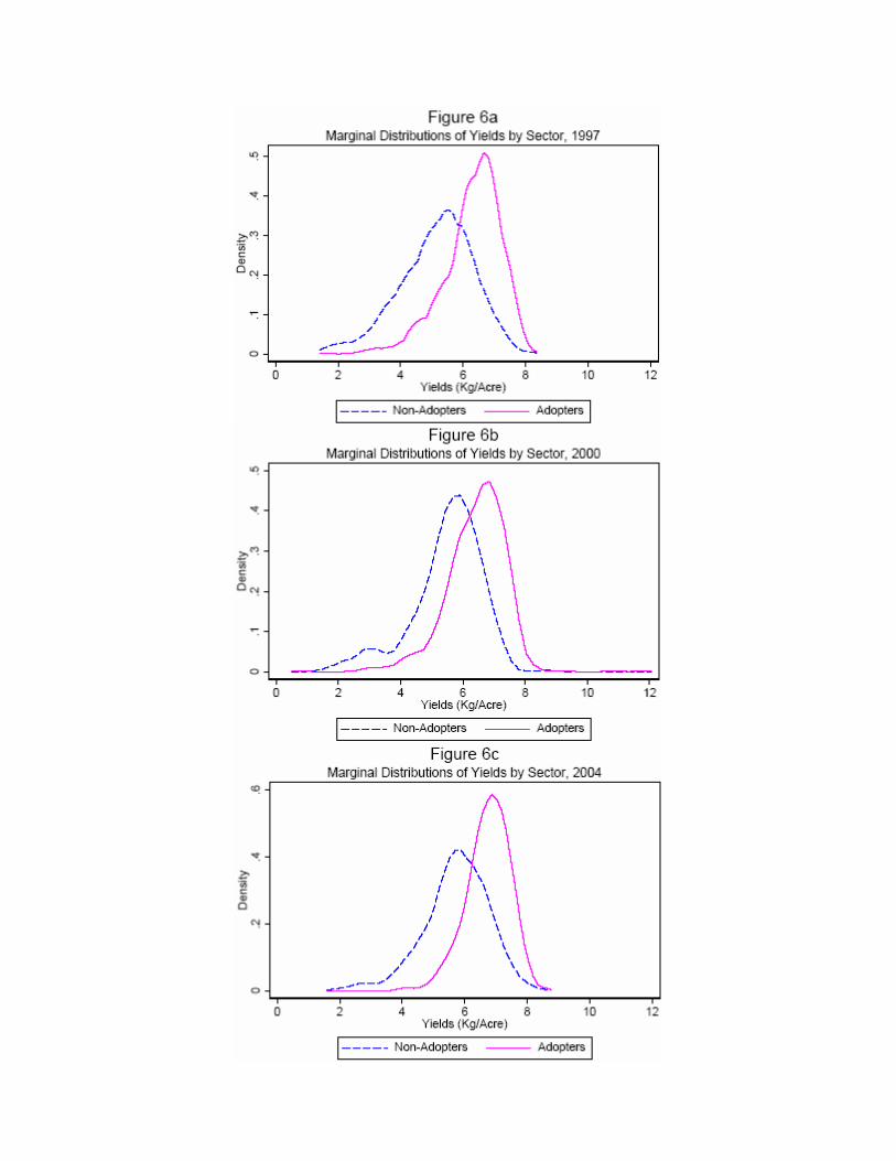
Table 1: Trends in Yields of Staples Average Annual % Changes in Yields (Hg/Ha), by Decade

1961-1970

1971-1980

1981-1990

1991-2004 Kenya Maize 0.362 2.373 1.169 -1.198 Wheat 5.646 2.333 -3.078 0.984 India Maize 1.502 0.842 1.900 2.572 Wheat 4.876 2.514 3.343 1.235 Rice 0.954 1.714 3.310 0.838 Mexico Maize 2.057 4.267 -0.548 1.447 Wheat 4.586 3.204 -0.255 1.664 Zambia Maize -0.267 10.403 1.571 -1.707

Source: FAOSTAT Online Database

Table 2a: Summary Statistics, by Sample Year

1997 Sample

2000 Sample

2004 Sample

Yield (Log Maize Harvest Per Acre) 5.907 (1.153) 6.125 (1.092) 6.350 (0.977) Acres Planted 1.903 (3.217) 2.313 (3.948) 1.957 (2.685) Total Seed Planted (Kg per Acre) 9.575 (7.801) 9.331 (6.805) 9.072 (6.863) Total Purchased Hybrid Planted (Kg per Acre) 6.273 (6.926) 5.918 (6.636) 5.080 (5.260) Total Local Seed Planted (Kg per Acre) 2.653 (6.326) 2.868 (6.129) 3.120 (7.318) Hybrid (dummy) 0.658 (0.475) 0.676 (0.468) 0.604 (0.489) Fertilizer (Kg DAP (di-ammonium phosphate) per Acre) 20.300 (38.444) 24.577 (79.919) 24.610 (34.001) Fertilizer (Kg MAP (mono-ammonium phosphate) per Acre) 1.566 (10.165) 0 (0) 0.308 (4.538) Fertilizer (Kg CAN (calcium ammonium nitrate) per Acre) 6.473 (24.727) 9.819 (75.081) 8.957 (21.702) Fertilizer (Kg NPK (nitrogen phosphorous potassium) per Acre) 4.256 (20.096) 2.365 (12.172) 1.217 (7.870) Total Fertilizer Expenditure (KShs per Acre) 1361.7 (2246.3) 1346.5 (3347.1) 1354.6 (1831.2) Land Preparation Costs (Kshs per Acre) 2168.1 (4895.7) 813.66 (1222.9) 808.99 (1080.2) Main Season Rainfall (mm) 620.83 (256.43) 599.10 (264.21) 728.11 (293.29)

Notes: Standard deviations in parentheses. KShs represents Kenyan shillings (the current exchange rate is on the order of 75 shillings to the US dollar). Henceforth, any variables measured in Kenyan shillings are deflated.

Source: TAMPA Project data.

Table 2b: Summary Statistics, by Hybrid/Non-Hybrid Use

1997 Sample

2000 Sample

2004 Sample

Hybrid Non-Hybrid Hybrid Non-Hybrid Hybrid Non-Hybrid No. of Households 791 411 813 389 726 476 Yield (Log Maize Harvest Per Acre)

6.296 (0.934)

5.158 (1.167)

6.423 0.948)

5.503 (1.113)

6.751 (0.692)

5.738 (1.030)

Total Maize Acres Cultivated 1.982

(3.557) 1.753

(2.428) 2.453

(4.334) 2.021

(2.970) 2.087

(3.029) 1.758

(2.042) Total Seed Planted (Kg per Acre)

9.669 (6.569)

9.394 (9.750)

20.628 (41.724)

9.926 (7.507)

8.746 (4.156)

9.569 (9.608)

Fertilizer (Kg DAP per Acre) 28.755

(44.115) 4.028

(13.266) 34.068

(95.214) 4.740

(14.638) 37.148

(37.294) 5.488

(13.909) Fertilizer (Kg CAN per Acre) 9.087

(29.715) 1.442

(7.152) 13.781

(90.809) 1.537

(9.479) 12.708

(24.961) 3.235

(13.622) Land Preparation Costs (KShs per Acre)

2006.0 (1316.2)

2480.1 (8168.4)

909.99 (1318.9)

614.43 (964.13)

918.44 (1095.2)

642.06 (1036.1)

Total Expenditure on Fertilizer (KShs per Acre)

1922.3 (2542.9)

282.64 (740.53)

1848.2 (3941.6)

297.80 (730.18)

1893.3 (1964.7)

533.09 (1211.4)

Main Season Rainfall (mm) 651.70

(228.82) 561.44

(293.88) 611.67

(270.44) 572.83

(249.00) 825.41

(215.20) 579.69

(332.05)

Notes: Standard deviations in parentheses. The mean of yields is higher and the standard deviation of yields lower in the hybrid sector. Source: TAMPA Project data.

Table 3: Basic OLS and Fixed Effects Specifications Dependent Variable is Yields (Log Maize Harvest Per Acre)

OLS, Pooled

OLS, Pooled

OLS, Pooled

FE

FE Hybrid 1.024 (0.033) 0.731 (0.034) 0.556 (0.035) 0.114 (0.052) 0.149 (0.049) Acres (x100) - - -0.385 (0.432) - -5.471 (0.839) Seed Kg per Acre (x10) - - 0.290 (0.020) - 0.272 (0.023) Land Preparation Costs per Acre (x10,000)

- - 0.216 (0.048) - 0.151 (0.054)

Main Season Rainfall (x1000) - - 0.688 (0.118) - 0.913 (0.112) Fertilizer per Acre (x1000) 0.052 (0.006) - 0.031 (0.007) Year = 1997 -0.199 (0.039) -0.205 (0.037) -0.272 (0.035) -0.216 (0.033) -0.289 (0.032) Year = 2004 0.299 (0.039) 0.278 (0.037) 0.131 (0.038) 0.233 (0.033) 0.089 (0.036) Constant 5.432 (0.036) 5.046 (0.072) 4.466 (0.085) 6.048 (0.042) -1.951 (4.931) Province Dummies No Yes Yes - - R-Squared 0.228 0.317 0.424 0.071 0.197

Notes: Standard errors are in parentheses. Omitted year is 2000. All regressions reported have 3600 observations. The covariates not reported above include labor variables and the average long term mean seasonal rainfall. The OLS and household fixed effects specifications run are respectively:

yit hit Xit′ it

yit i hit Xit′ it

Source: TAMPA Project data.

Table 4: CRE Model Reduced Forms and Structural Estimates Dependent Variable is Yields (Log Maize Harvest Per Acre)

Reduced Forms Without Covariates

Reduced Forms With Covariates Yields, 1997 Yields, 2000 Yields, 2004 Yields, 1997 Yields, 2000 Yields, 2004 Hybrid, 1997 0.574 (0.075) 0.345 (0.084) 0.467 (0.067) 0.401 (0.168) 0.252 (0.071) 0.351 (0.057) Hybrid, 2000 0.323 (0.081) 0.424 (0.086) 0.230 (0.074) 0.233 (0.071) -0.022 (0.176) 0.161 (0.058) Hybrid, 2004 0.680 (0.080) 0.490 (0.081) 0.632 (0.070) 0.407 (0.071) 0.360 (0.073) 0.292 (0.147)

Standard CRE Model Structural Estimates β λ1 λ2 λ3 χ2

5 (p-value) OMD, Without covariates 0.071 (0.054) 0.498 (0.053) 0.281 (0.056) 0.502 (0.059) 100.87 (0.000) EWMD, Without covariates 0.117 (0.054) 0.475 (0.053) 0.275 (0.056) 0.503 (0.059) - OMD, With covariates 0.147 (0.046) 0.362 (0.042) 0.208 (0.044) 0.328 (0.045) 16.315 (0.006) EWMD, With covariates 0.168 (0.046) 0.344 (0.042) 0.210 (0.044) 0.338 (0.045) -

Notes: Standard errors are in parentheses. Reduced forms are estimated with and without covariates (acreage, real fertilizer expenditure, land preparation costs, seed, labor and rainfall variables). All covariates are assumed to be exogenous for the estimation. The following reduced form for each t is estimated:

yit t 1thi1 2thi2 3thi3 Xi′t it

where hi1, hi2 and hi3 indicate hybrid use in each period. Only reduced form coefficients for the hybrid history are reported. The structural equation is: yit hit i uit

The projection used by the CRE model, in conjunction with the reduced form estimates, to estimate the structural model by minimum distance is: i 0 1hi1 2hi2 v i

Structural coefficients reported: β and projection coefficients (λ’s). OMD and EWMD are optimal (weighted by inverted reduced form variance-covariance matrix) and equally weighted minimum distance respectively. χ2 statistic on the overidentification test is the value of the OMD minimand.

Source: TAMPA Project data.

Table 5: Selection Returns by Hybrid History (Joiners, Leavers and Stayers)

Dependent Variable is Yields (Log Maize Harvest Per Acre)

1997-2000

2000-2004

1997-2004

Variable

1997 Yield 2000 Yield 2000 Yield 2004 Yield 1997 Yield 2004 Yield Without Covariates

Hybrid Stayers 1.411

(0.070) 1.109

(0.070) 1.132

(0.067) 1.172

(0.057) 1.505

(0.066) 1.280

(0.056) Leavers 0.746

(0.112) 0.281

(0.110) 0.426

(0.095) 0.332

(0.081) 0.809

(0.094) 0.648

(0.079) Joiners 0.563

(0.105) 0.430

(0.104) 0.403

(0.127) 0.693

(0.108) 1.007

(0.114) 0.883

(0.096)

With Covariates Hybrid Stayers 0.766

(0.073) 0.637

(0.075) 0.719

(0.073) 0.593

(0.061) 0.868

(0.074) 0.652

(0.063) Leavers 0.466

(0.097) 0.044

(0.100) 0.367

(0.086) 0.159

(0.067) 0.509

(0.085) 0.350

(0.069) Joiners 0.316

(0.089) 0.335

(0.094) 0.258

(0.115) 0.339

(0.092) 0.491

(0.101) 0.499

(0.084)

Notes: Standard errors are in parentheses. In each year, the following regression is run both with and without the standard set of Xi covariates used previously: yi 1hi11 2hi10 3hi01 Xi

′ ui

where hi11 is the dummy indicating that farmer i is a hybrid stayer (plants hybrid in both periods), hi10 indicates he is a leaver (plants hybrid the first year, not the second), hi01 indicates he is a joiner (plants hybrid the second year, not the first). The coefficients reported are µ1, µ 2 and µ 3.

Source: TAMPA Project data.

Table 6: Heterogeneity by Observables Returns in the Hybrid/Non-Hybrid Sector

Dependent Variable is Yields (Log Maize Harvest Per Acre)

OLS, with Covariates

FE, with Covariates

Variable

Hybrid Non-Hybrid Hybrid Non-Hybrid Acreage (x 100) 0.784

(0.438) -5.427 (1.125)

-4.353 (0.917)

-8.360 (2.013)

Total Seed Planted (Kg per Acre) (x 100)

3.418 (0.279)

2.176 (0.307)

2.854 (0.323)

2.397 (0.401)

Land Preparation Costs per Acre (KShs) (x 10,000)

0.487 (0.129)

0.216 (0.031)

0.523 (0.170)

0.151 (0.068)

Total Fertilizer Expenditure per Acre (KShs) (x 10,000)

0.430 (0.055)

1.855 (0.305)

0.245 (0.064)

1.176 (0.534)

Main Season Rainfall (mm) (x 10,000)

3.879 (1.399)

12.286 (2.261)

9.297 (1.416)

12.706 (2.599)

Average Return (β) when Returns Vary by Observables (evaluated at mean X’s)

0.473 (0.041)

0.132 (0.054)

Number of Observations 2330 1276 2330 1276

Notes: Standard errors in parentheses. The following specification is estimated separately for the sample of farmers who use hybrid and non-hybrid maize: yit

j j Xtij itj j ∈ H,N

The covariates included that are not reported are labor variables, province dummies, year dummies and the average main seasonal rainfall. Source: TAMPA Project data.

Table 7: Two Period Comparative Advantage CRC Model Reduced Form Estimates Dependent Variable is Yields (Log Maize Harvest Per Acre)

Reduced Forms Without Covariates

Reduced Forms With Covariates

Yields, 1997 Yields, 2004 Yields, 1997 Yields, 2004 Hybrid, 1997 0.809 (0.094) 0.648 (0.079) 0.747 (0.087) 0.508 (0.072) Hybrid, 2004 1.007 (0.114) 0.883 (0.096) 0.706 (0.106) 0.704 (0.089) Hybrid 1997*Hybrid 2004 -0.311 (0.142) -0.252 (0.120) -0.273 (0.130) -0.262 (0.107) Acres (x10) - - 0.165 (0.080) -0.001 (0.081) Hired Labor Cost per Acre (x 10,000) - - 0.188 (0.085) 0.122 (0.017) Family Labor Cost per Acre (x 10,000) - - 0.139 (0.049) 0.559 (0.098) Seed Kg per Acre (x 10) - - 0.254 (0.038) 0.276 (0.033) Land Preparation Cost per Acre (x 10,000) - - 0.186 (0.055) 0.511 (0.201) Main Season Rainfall per Acre (x 1000) - - 0.817 (0.104) 0.449 (0.083) Fertilizer Expenditure per Acre (x 10,000) - - 0.873 (0.126) 0.704 (0.127) No of Observations 1202 1202 1202 1202 R-Squared 0.303 0.307 0.429 0.457

Notes: Standard errors are in parentheses. Reduced forms are estimated with and without covariates (all covariates reported). Reduced forms are for the case where all covariates are exogenous: only hybrid is correlated with the comparative advantage, θi. See Table 7b for projection and structural estimates.

Source: TAMPA Project data.

Table 8a: Two Period Comparative Advantage CRC Model Structural Estimates Dependent Variable is Yields (Log Maize Harvest Per Acre)

With Only Hybrid Endogenous

Without Covariates With Covariates

EWMD OMD EWMD OMD

λ1 0.786 (0.068) 0.743 (0.068) 0.648 (0.059) 0.596 (0.059) λ2 0.963 (0.093) 1.030 (0.093) 0.711 (0.085) 0.772 (0.085) λ3 -5.4185 (30.55) -1.622 (0.724) -1.098 (1.284) -0.930 (0.256) β 3.034 (16.76) 1.008 (0.274) 0.804 (0.324) 0.733 (0.048) ф -1.104 (0.700) -1.558 (0.533) -1.740 (2.235) -1.966 (0.906)

χ2

1 (p-value) - 71.63 (0.000) - 63.75 (0.000)

Notes: Standard errors are in parentheses. The reduced forms for these estimates are reported in Table 7 (for the case where only the hybrid decision is endogenous, i.e. correlated with the θi’s). The projection used in this model is:

i 0 1hi1 2hi2 3hi1hi2 v i The minimum distance estimations are run for both cases with and without covariates (all the covariates are reported in Table 7 above). The structural coefficients reported are the average return to hybrid (β), the comparative advantage coefficient (ф), and all the projections coefficients (the λ’s). OMD and EWMD are optimal (weighted by inverted reduced form variance-covariance matrix) and equally weighted minimum distance respectively. The χ2 statistic on the overidentification test is the value of the OMD minimand.

Source: TAMPA Project data.

Table 8b: Two Period Comparative Advantage CRC Model Structural Estimates Dependent Variable is Yields (Log Maize Harvest Per Acre)

With Both Fertilizer and Hybrid as Endogenous

Without Covariates With Covariates

EWMD OMD EWMD OMD

β -0.129 (0.161) -0.701 (1.312) 0.584 (0.791) 0.717 (0.042) ф -0.468 (0.145) -0.824 (0.224) -0.783 (0.691) -1.807 (0.460)

χ2

8 (p-value) - 64.70 (0.000) - 110.32 (0.000)

With a Joint Fertilizer-Hybrid Decision

Without Covariates With Covariates

EWMD OMD EWMD OMD

β 0.070 (0.127) -0.007 (0.312) 0.114 (0.068) 1.288 (4.297)

ф 0.179 (0.882) -0.576 (0.455) -0.3052 (1.029) -1.100 (0.480) χ2

1 (p-value) - 33.01 (0.000) - 40.62 (0.000)

Notes: Standard errors are in parentheses. Reduced forms are not reported. Upper panel reports structural estimates of the average return to hybrid (β) and the comparative advantage coefficient (ф) for the case of endogenous hybrid and fertilizer use (with and without exogenous covariates). Projection used is:

i 0 1hi1 2hi2 3hi1hi2 4hi1 f i1 5hi2 f i1 6hi1hi2 f i1 7hi1 f i2 8hi2 f i2 9hi1hi2 f i2 10 f i1 11 f i2 v i The lower panel shows the results from treating the fertilizer-hybrid decision as joint such that a technology sector is defined as when both hybrid and

fertilizer are used and not otherwise. The reduced forms, structural coefficients and projection are identical to the case reported in Table 8a. Only two structural coefficients are reported: the average return to hybrid (β) and the comparative advantage coefficient (ф). The covariates include acreage, land preparation costs, seed, labor and rainfall variables, and the intensive margin of fertilizer use (total real expenditure) as exogenous variables.

Source: TAMPA Project data.

Table 9: Three Period CRC Model Structural Estimates (all with Covariates) Dependent Variable is Yields (Log Maize Harvest Per Acre)

Hybrid Decision

Joint Hybrid-Fertilizer Decisions

OMD EWMD OMD EWMD λ1 0.361 (0.048) 0.247 (0.045) 0.465 (0.055) 0.441 (0.055) λ2 0.165 (0.049) 0.140 (0.048) 0.225 (0.057) 0.245 (0.057) λ3 0.275 (0.094) 0.232 (0.067) 0.216 (0.066) 0.206 (0.065) λ4 0.081 (0.111) -0.008 (0.093) -0.165 (0.124) -0.235 (0.124) λ5 -0.115 (0.132) -0.142 (0.090) -0.209 (0.122) -0.233 (0.121) λ6 0.221 (0.137) 0.078 (0.112) -0.116 (0.101) -0.278 (0.096) λ7 -0.259 (0.178) -0.116 (0.138) -0.080 (0.176) 0.059 (0.185) β 0.093 (0.050) 0.295 (0.042) 0.128 (0.053) 0.183 (0.070) ф -0.144 (0.124) 0.685 (0.349) -0.327 (0.170) -0.246 (0.269)

χ212 (p-value) 95.04 (0.000) - 151.40 (0.000) -

Notes: Standard errors in parentheses. All specifications reported above in this table include the following set of covariates: acreage, real fertilizer expenditure,

land preparation costs, seed, labor and rainfall variables. Here, all the covariates are treated as exogenous in terms of being correlated with the comparative advantage component, θi. Note that in case of the joint hybrid-fertilizer decision, sector choice is defined by the use of fertilizer. However, the covariates include the intensive margin of use (i.e. the total real expenditure on fertilizer) as a control (exogenous, conditional on extensive margin).

Source: TAMPA Project data.

Table 10: Heckit and Treatment Effect Estimates under Non-Random Assignment (ATE, TT, MTE, LATE) Dependent Variable is Yields (Log Maize Harvest Per Acre)

Heckman Two-Step Estimates

Implied Treatment Effects

Year Selection Correction λ Hybrid Sector

Selection Correction λ Non-Hybrid Sector

ATE

TT

MTE Slope

1997 -0.871 (0.171) 0.897 (0.756) 2.097 1.374 -1.769 (0.775)

2000 -0.861 (0.119) -0.639 (0.350) 0.756 0.677 -0.222 (0.370)

2004 -0.910 (0.192) 0.001 (0.162) 1.346

0.830 -0.911 (0.251)

IV (LATE) Estimates (Conditional on Covariates)

First Stage: Effect of Distance on Probability of Using Hybrid Second Stage: Effect of Predicted Hybrid on Yields

-0.516 (0.097)

1.543 (0.434)

Notes: Standard errors are in parentheses. All regressions control for the same set of covariates as previously. The first two upper panel columns show (for

each year) the two-step selection corrected estimates of coefficients on the Inverse Mills ratio for hybrid and non-hybrid sectors from: hi Zi

′ ui

s

yiH Xi

′H H Zi

′/Zi′ and yi

N Xi′N N Zi

′/ 1 − Zi′

The third column reports the average treatment effect accounting for the selection (it takes the predicted yields from the second step in each sector subtracts out the effect of the selection term and reports the difference in this predicted value across the two sectors). The treatment on the treated is reported next which looks at the difference in the second step predicted yields (including the selection terms) between the two sectors only for the sample of farmers who plant hybrid. Finally, the MTE slope is just the difference in the λ coefficients for the hybrid and non-hybrid selection terms (the difference between coefficients reported in the first two columns). ATE, TT, MTE are all evaluated at the mean Xi’s. The lower panel reports the IV estimates which use distance to closest fertilizer supplier (not where fertilizer is purchased) as an IV for the hybrid decision in the second stage:

yit hit Xi

′ uit where

hit 0

Dist Xi′

IV results are roughly the same if excluded instruments are distance interacted with wealth quantiles, controlling for distance and wealth in both stages. Source: TAMPA Project data.

Table 11: The Adoption Decision Revisited Dependent Variable is Use of Hybrid

Linear Probability Models

Fixed Effects Model

CRC Model

(1) (2) (3) (4) (5) (6) Predicted Fixed Effects from Household Fixed Effects Model

-0.053 (0.007)

0.182 (0.011)

- - - -

Predicted θi’s - - 0.199

(0.031) 0.344

(0.029) - -

Predicted τi’s - - - - -0.041

(0.015) -0.020 (0.014)

Covariates No Yes No Yes No Yes Province Dummies Yes Yes Yes Yes Yes Yes Year Dummies Yes Yes Yes Yes Yes Yes

Notes: Standard errors are in parentheses. This table reports linear probability models of the adoption decision. The first two columns report how the predicted fixed effects from the following fixed effects model correlate with the decision to adopt hybrid maize, and how this correlation changes with covariates.

yit hit Xit′ Xit

′ hit i it Columns (3) through (5) cover a similar exercise, this time look at the estimates of the predicted θi’s and τi’s and how well they correlate with the

adoption decision. The set of covariates here includes acreage, real fertilizer expenditure, land preparation costs, seed, labor and rainfall variables. Source: TAMPA Project data.

Table 12: OLS and FE Estimates by Predicted Fertility Quartile Dependent Variable is Yields (Log Maize Harvest Per Acre)

Predicted Fertility Quartile

1

2

3

4

OLS Estimate of Hybrid Return 0.418

(0.082) 0.403

(0.072) 0.473

(0.062) 0.347

(0.077) FE Estimate of Hybrid Return 0.150

(0.105) 0.267

(0.099) 0.155

(0.082) 0.056

(0.099) Hybrid Prevalence 31.01 59.00 78.85 89.67 Number of Observations 903 900 903 900

Notes: Standard errors are in parentheses. This table shows the OLS and household FE estimates of the return to hybrid and the prevalence of hybrid use across what I refer to as predicted fertility quartiles. Using only the sample of non-hybrid farmers in 1997, I estimate the expected yield based on the entire set of covariates (acreage, real fertilizer expenditure, land preparation costs, seed, labor and rainfall variables and province and year dummies). I then predict what the expected yield under traditional varieties would be for those planting hybrid. I call this predicted value the index of fertility for my entire sample of farmers. This table therefore look across the quartiles of this estimated fertility measure, comparing the OLS and FE estimates of the hybrid yield return and the prevalence of hybrid. Similar patterns hold out when looking at quantile regressions. Note that the predicted fixed effects come from the three period problem (estimates reported in Table 3), but similar results hold for the two period problem. And, the predicted θi’s used are for the two period case where both hybrid and fertilizer use are considered endogenous (estimates reported in the last column of the upper panel of Table 8b).

Source: TAMPA Project data.

Table 13: Correlates of Estimated θi’s Dependent Variable is the Estimated θi’s

(1)

(2)

(3)

(4) Distance to Closest Fertilizer Seller (x100) -0.339 (0.103) -0.324 (0.105) -0.303 (0.108) -0.305 (0.108) Fraction of Household with No Education (x10) -0.495 (0.261) 0.247 (0.376) 0.210 (0.373) 0.195 (0.374) Distance to Tarmac Road (x100) -0.181 (0.089) -0.215 (0.091) -0.196 (0.095) -0.188 (0.095) Distance to Matatu Stop (x100) 0.075 (0.267) 0.288 (0.277) 0.039 (0.280) 0.010 (0.280) Distance to Motorable Road (x100) -0.704 (0.438) -0.567 (0.447) -0.001 (0.453) -0.017 (0.454) Tried to Get Credit (x10) - - 0.017 (0.139) - Received Credit (x10) -0.145 (0.132) - - -0.023 (0.145) Dummies for Household Head Education (P value on Joint Significance of these Dummies)

No Yes (0.03)

Yes (0.04)

Yes (0.03)

Province Dummies No No Yes Yes Year Dummies No No Yes Yes

Notes: Standard errors are in parentheses. This table reports the correlations of the predicted θi’s with various observables in my dataset, namely distance from the household to the closest fertilizer seller, fraction of adult household members with no education, distance to the closest tarmac road, distance to the closest matatu (public transport) stop, distance to the closest motorable road, a dummy for whether the household tried to get credit, a dummy for whether the household received any credit, dummies for education of the household head, province and year dummies, depending on the specification. The predicted θi’s used are from the two period case with endogenous hybrid and fertilizer use (last column of the upper panel of Table 8b).

Source: TAMPA Project data.

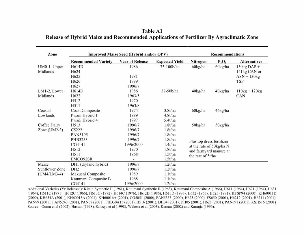
Table A1 Release of Hybrid Maize and Recommended Applications of Fertilizer By Agroclimatic Zone

Improved Maize Seed (Hybrid and/or OPV)

Recommendations

Zone

Recommended Variety Year of Release Expected Yield Nitrogen P2O5 Alternatives UM0-1, Upper Midlands

H614D H624 H625 H626 H627

1986 -

1981 1989

1996/7

75-100b/ha 60kg/ha 60kg/ha 130kg DAP + 141kg CAN or ASN + 130kg TSP

LM1-2, Lower Midlands

H614D H622 H512 H511

1986 1963/5 1970

1963/8

37-50b/ha 40kg/ha 40kg/ha 110kg + 120kg CAN

Coastal Lowlands

Coast Composite Pwani Hybrid 1 Pwani Hybrid 4

1974 1989 1997

3.8t/ha 4.8t/ha 5.4t/ha

60kg/ha 46kg/ha

50kg/ha 50kg/ha

Coffee Dairy Zone (UM2-3)

H513 C5222 PAN5195 PHB3253 CG4141 H512 H511 EMCO92SR

1996/7 1996/7 1996/7 1996/7

1996/2000 1970 1968

-

1.8t/ha 1.8t/ha 1.8t/ha 1.8t/ha 1.4t/ha 1.8t/ha 1.5t/ha 1.5t/ha

Plus top dress fertilizer at the rate of 50kg/ha N and farmyard manure at the rate of 5t/ha

Maize Sunflower Zone (UM4/LM3-4)

DH1 (dryland hybrid) DH2 Makueni Composite Katumani Composite B CG4141

1996/7 1996/7 1989 1968

1996/2000

1.2t/ha 1.2t/ha 1.1t/ha 1.1t/ha 1.2t/ha

Additional Varieties (Yr Released): Kitale Synthetic II (1961), Katumani Synthetic II (1963), Katumani Composite A (1966), H611 (1964), H621 (1964), H631 (1964), H611C (1971), H612C (1966), H613C (1972), H614C (1976), H612D (1986), H613D (1986), H632 (1965), H525 (1981), KTSP94 (2000), KH60011D (2000), KH634A (2001), KH60015A (2001), KH60016A (2001), CG5051 (2000), PAN5355 (2000), H623 (2000), FS650 (2001), H6212 (2001), H6211 (2001), PAN99 (2001), PAN5243 (2001), PAN67 (2001), PHB30A15 (2001), H516 (2001), DH04 (2001), DH05 (2001), H628 (2001), PAN691 (2001), KSH516 (2001) Source: Ouma et al (2002), Hassan (1998), Salasya et al (1998), Wekesa et al (2003), Kamau (2002) and Karanja (1996).

Table A2: Impact Distribution Percentiles

Perfect Positive Dependence

Perfect Negative Dependence

Percentile 1997 2000 2004 Joiners Leavers 1997 2000 2004 Joiners Leavers

5 1.386 1.644 1.579 0.186 0.218 -2.485 -2.227 -1.743 -3.015 -3.183 (0.191) (0.222) (0.167) (0.318) (0.287) (0.106) (0.155) (0.102) (0.204) (0.211)

10 1.609 1.260 1.458 0.440 -0.084 -1.358 -1.434 -1.101 -2.304 -2.658 (0.186) (0.255) (0.132) (0.204) (0.265) (0.149) (0.112) (0.095) (0.179) (0.217)

25 1.386 0.862 1.139 0.287 0.105 0.000 -0.386 -0.113 -1.071 -1.174 (0.111) (0.113) (0.097) (0.131) (0.161) (0.090) (0.056) (0.077) (0.126) (0.114)

50 1.253 0.916 0.976 0.068 0.258 1.253 0.916 0.976 0.068 0.258 (0.099) (0.077) (0.083) (0.106) (0.121) (0.085) (0.067) (0.072) (0.106) (0.121)

75 1.012 0.768 0.827 0.028 0.191 2.398 2.016 2.079 1.386 1.471 (0.104) (0.065) (0.084) (0.092) (0.085) (0.101) (0.107) (0.084) (0.103) (0.143)

90 0.811 0.777 0.584 0.027 0.043 3.778 3.470 3.143 2.771 2.617 (0.111) (0.093) (0.088) (0.066) (0.114) (0.137) (0.235) (0.111) (0.131) (0.214)

95 0.511 0.624 0.560 0.074 0.065 4.382 4.495 3.881 3.275 3.466 (0.106) (0.083) (0.087) (0.146) (0.146) (0.177) (0.168) (0.143) (0.282) (0.270)

0.261 0.240 0.340 0.129 0.138 1.988 1.885 1.634 1.867 1.986 Impact Std Deviation (0.043) (0.057) (0.045) (0.043) (0.064) (0.049) (0.056) (0.043) (0.076) (0.087)

0.994 0.993 0.997 0.996 0.992 -0.943 -0.907 -0.969 -0.947 -0.942 Outcome Correlation (0.004) (0.004) (0.002) (0.010) (0.005) (0.011) (0.014) (0.009) (0.026) (0.016)

Notes: The impact standard deviation is the standard deviation of the percentile differences. The outcome correlation is the correlation of the two percentiles of

the two distributions. Bootstrap standard errors are in parentheses. The 1997, 2000 and 2004 are cross-sectional results, and the joiners and leavers results are the household fixed effects versions. A test of whether the impact standard deviation is significantly different from zero tests the null:

H0 : qyH − qyN k for all q such that 0 ≤ q ≤ 100