sdtic · sdtic_ selecte s aug 2 a1 1992 d11 ... alur, evan cohn, anil gangolli, aaron goldberg,...
TRANSCRIPT
77June 1991 4 Report No. STAN-CS-91-1366
Thesis
AD-A254 553
Combinatorial Algorithms for Optimization Problems
by
Edith Cohen
SDTIC_SELECTE
S AUG 2 1 1992 D11A
Department of Computer Science
Stanford University
Stanford, California 94305
* his- docmuent has been opprovdfor public reiese a d sole; itsdictribution is unlinited.
N 92-23193.. 1q0
REPORT DOCUMENTATION PAGE '"
I~M Uft Aaaftaw"e~mumq~,,~uminalsgm amp g,
1.~~~m0aE m AWC V51GMT"amnNO ILsW IAT 4VW T
7. PIN IUNG:: ORGANIZATION-- N*AR"(t) AND -*-04iiSKl) L f, OIAIZT"r, Ib':j
H.STGiOING/ MONITOWUNG AGENCT NAMI|I) AND AGGMISSRIS) II).SPONSONNlulOITONN;H
ON1C A V 000 14
I . SUPPlNl5 MOT1S
Ila. OITAMtUTiO I AVA INUT STATEMENT 1116 OISTUR OANN C00 O,1|, III.I C- ;
Abstract. Linear programming is a very general and widely used framework. In this thesis we consider
several combinatorial optimisation problems that can be viewed as classes of linear programming problems
with special structure. It is known that polynomial time algorithms exist for the general linear programming
problem. It is not known, however, whether any of them are strong polynomial In addition, it seems that
the general problem is inherently sequential. For problems with special structure, our goals are to develop
sequential and parallel algorithms that are faster than those known for general linear programming and to
determine whether strongly polynomial algorithms exist. (i) We develop a technique that extends the classesof problems known to have strongly polynomial algorithms, or known to be quickly solvable in parallel. This
technique is used to obtain a fast parallel algorithm and a strongly polynomial algorithm for detecting
cycles in periodic graphs of fixed dimension. We mention additional applications to parametric extensions of
problems where the number of parameters is fixed. (ii) We introduce algorithms for solving linear systemswhere each inequality involves at most two variables. These algorithms improve over the sequential and
parallel running times of previous algorithms. These results are combined with additional ideas to yield
faster algorithms for some generalised network flow problems.
14. SuWJECT TIRMS 15 NUMER OF PAGES
M PUO CODE
I?. SECURITY CLASSIFICATION 16. SECURITY CLASSifICATION 1. SECUMITY CLASSiFICATION U ATION OF AIS T' A
OF REPO"Tof TwoS PAGE Of ABSTRACT
'SIN 7O.OI.IK.SSO0 Stengeat Owm 619 e!.0-06- " m ..4.,A ,I 'It a
/
COMBINATORIAL ALGORITHMS
FOR OPTIMIZATION PROBLEMS
A DISSERTATION
SUBMITTED TO THE DEPARTMENT OF COMPUTER SCIENCE
AND THE COMMITTEE ON GRADUATE STUDIES
OF STANFORD UNIVERSITY
IN P.:' TIAL FULFILLMENT OF THE REQUIREMENTS
FOR THE DEGREE OF D : tr5,LMTrry ( UPEUD 5
DOCTOR OF PHILOSOPHY
Accesion ForNreS CRA&I
OTIC TABUnarVIOW'rced 1Justification
By Dist ibutiorEdith Cohen ~-
June 1991 0:; A.~~ISDTIC QUAITY 'rru4wx8
( Copyright 1991 by Edith Cohen
All Rights Reserved
i
I certify that I have read this dissertation and that in my
opinion it is fully adequate, in scope and in quality, as a
dissertation for the degree of Doctor of Philosophy.
Andrew V. Goldberg(Principal Adviser)
I certify that I have read this dissertation and that in my
opinion it is fully adequate, in scope and in quality, as a
dissertation for the degree of Doctor of Philosophy.
Nimrod Megiddo
I certify that I have read this dissertation and that in my
opinion it is fully adequate, in scope and in quality, as a
dissertation for the degree of Doctor of Philosophy.
Serge A. Plotkin
Approved for the University Committee on Graduate
Studies:
Dean of Graduate Studies
olom
Abstract
Linear programming is a very general and widely used framework. In this thesis we
consider several combinatorial optimization problems that can be viewed as classes
of linear programming problems with special structure. It is known that polynomial
time algorithms exist for the general linear programming problem. It is not known,
however, whether any of them are strongly polynomial (informally, a polynomial time
algorithm is strongly polynomial if the number of arithmetic operations performed is
bounded by a polynomial function of the number of variables and inequalities, i.e., is
independent of the size of the numbers). In addition, it seems that the general problem
is inherently sequential (fast parallel algorithms cannot be obtained). For problems
with special structure, our goals are to develop sequential and parallel algorithms
that are faster than those known for general linear programming and to determine
whether strongly polynomial algorithms exist.
We develop a technique that extends the classes of problems known to have
strongly polynomial algorithms, or known to be quickly solvable in parallel. This tech-
nique is used to obtain a fast parallel algorithm and a strongly polynomial algorithm
for detecting cycles in periodic graphs of fixed dimension. We mention additional
applications to parametric extensions of problems where the number of parameters is
fixed.
We introduce algorithms for solving linear systems where each inequality involves
at most two variables. These algorithms improve over the sequential and parallel
running times of previous algorithms. These results are combined with additional
ideas to yield faster algorithms for some generalized network flow problems.
iv
To my parents Amy arid Eliahu ~ ' in
my sister Mirzt n,~'ix
and my brother Menashe vwith all my love lfX
Acknowledgement s
I would like to thank the three members of my committee: my advisor Andrew Gold-
berg for suggesting research problems and offering advice, Nimrod Megiddo for closely
working with me and guiding me to become an independent researcher, and Serge
Plotkin for carefully reading this thesis and sharing numerous interesting ideas.
I would also like to thank Christos Papadimitriou, my advisor during my first year,
and Ernst Mayr for early guidance; Leo Guibas and Rajeev Motwani for interesting
classes; Don Knuth and Alex Schiffer for their advice; the people of IBM Almaden
for giving me the opportunity to spend there fruitful and enjoyable time throughout
my PhD studies; and Adam Grove, Toma's Feder, Vwani Roychowdhury, Eva Tardos,
Steve Vavasis, and Pete Veinott for beneficial discussions related to my thesis work.
I would like to mention, in random order, Alex Wang, Tom Henzinger, Greg Plax-
ton, Tomek Radzik, Shoshi Wolf, Inderpal Mumick, Yossi Friedman, Gidi Avrahami,
Daphne Koller, Alon Levy, Efi Fogel, Eran Yehudai, Sherry Listgarten, Tim Fer-
nando, Misha Kharitonov, David Cyrluk, Yossi Azar, Moni Naor, Seffi Naor, Rajeev
Alur, Evan Cohn, Anil Gangolli, Aaron Goldberg, Ramsey Haddad, Robert Kennedy,Dror Maydan, Steven Phillips, Martin Rinard, Ken Ross, Shaibal Roy, David Salesin,
Ashok Subramanian, and Orli Waarts.
For the fantastic period I had at Stanford I am most grateful to my best friend Ling,
to the people mentioned above, and to the Sierras, the Pacific, and the California
sun.
Last, I am obliged to my parents for encouraging my curiosity, revealing to me
the joy and satisfaction of learning and understanding, and giving me the confidence
and stubbornness needed to pursue my ideas and goals.
vi
Contents
Abstract iv
Acknowledgements vi
1 Introduction 1
1.1 Background ........ ................................ 1
1.2 Outline of the thesis ...... ........................... 4
1.3 Notation ........ .................................. 7
2 Detecting cycles in periodic graphs 10
2.1 Introduction ........ ................................ 11
2.2 Preliminaries ........ ............................... 14
2.3 An overview ........ ................................ 15
2.4 Detecting zero-cycles ....... ........................... 18
2.4.1 Computing a witness or a separating vector ............. 21
2.4.2 Computing the partition .......................... 22
2.4.3 The algorithm .................................. 26
2.5 Geometric lemmas. ................................... 28
2.6 Applications of the zero-cycle detection algorithm .............. 30
vii
2.6.1. Scheduling .. .. .. .. ... ... ... ... ... ... ..... 31
2.6.2 Strong connectivity. .. .. .. .. ... .... ... ... .... 34
2.7 Concluding remarks .. .. .. .. .. .... ... ... ... ... .... 35
3 Parametric minimum cycle 37
3.1 Preliminaries. .. .. ... ... ... ... ... ... ... .... .. 38
3.1.1 The oracle problem. .. .. .. .. .... ... ... ... .... 42
3.1.2 Geometric lemmas .. .. .. ... ... ... ... ... ..... 44
3.1.3 Back to zero-cycles. .. .. .. ... ... ... ... ... ... 50
3.2 Algorithm for parametric min cycle-mean .. .. .. .. .. .... .... 51
3.3 Algorithm for parametric minimum cycle .. .. .. .. ... ... .... 55
3.3.1 Hyperplane queries. .. .. .. ... ... ... ... ... .... 57
3.3.2 Employing multi-dimensional search .. .. .. .. .. ... ... 59
3.3.3 Algorithm for extended parametric minimum cycle. .. .. ... 62
3.3.4 Correctness. .. .. .. ... ... ... .... ... ... .... 64
3.3.5 Complexity. .. .. .. ... ... .... ... ... ... .... 65
4 Convex optimization in fixed dimension 67
4.1 Introduction .. .. .. .. ... ... ... ... ... .... ... .... 68
4.2 Preliminaries. .. .. ... ... ... ... ... ... ... .... .. 68
4.3 Hyperplane queries. .. .. .. ... ... ... ... ... ... ..... 74
4.4 Employing multi-dimensional search .. .. .. .. .. .... ... .... 76
4.5 The algorithm. .. .. .. .. ... .... ... ... ... ... ..... 78
4.6 Correctness. .. .. .. ... ... ... .... ... ... ... ..... 79
4.7 Complexity. .. .. .. ... .... ... ... ... ... ... ..... 80
4.8 Parametric extensions of problems. .. .. .. .. ... ... ... ... 81
Vii
-',7, 31 -11 '777 -- >. 7P 7- F
5 Systems with two variables per inequality 84
5.1 Introduction .. .. .. .. ... ... ... ... .... ... ... .... 84
5.2 Preliminaries. .. .. ... ... ... ... ... ... .... ... .. 87
5.2.1 The associated graph .. .. .. .. ... ... .... ... .... 87
5.2.2 Pushing bounds along edges .. .. .. .. .... ... ... .. 90
5.2.3 Properties of the feasible region .. .. .. .. .... ... .... 92
5.2.4 Characterizations of TVPI polyhedra. .. .. .. ... ... .. 94
5.2.5 Locating values .. .. .. ... ... ... ... ... ... .... 97
5.3 The basic algorithm. .. .. .. .. ... ... ... ... ... ...... 104
5.3.1 The framework. .. .. .. ... ... .... ... ... ..... 105
5.3.2 Correctness .. .. .. ... ... ... ... ... ... ... .. 108
5.3.3 Complextity of the naive implementation .. .. .. .. ... .. 110
5.3.4 Solving TVPI systems by locating pools of values. .. .. .... 111
5.4 Algorithms for locating a pool. .. .. .. ... ... ... ... ..... 112
5.4.1 0(n) time using 0(nm) processors. .. .. ... ... ... .. 112
5.4.2 Overview of a 6(mn) algorithm. .. .. .. ... ... ... .. 114
5.5 Locating the strongly infeasible values. .. .. ... ... ... .... 115
5.5.1 The algorithm .. .. .. .. ... ... ... ... ... ... .. 116
5.5.2 Probability for a successful iteration of Loop A. .. .. .. .. 118
5.5.3 The "check" procedure. .. .. .. ... ... ... ... ..... 121
5.5.4 Properties of the "check" procedure .. .. .. .. ... ... .. 122
5.5.5 Estimating the number of big values. .. .. ... ... ..... 124
5.6 Locating weakly infeasible and feasible values .. .. .. ... ... .. 127
5.6.1 The algorithm .. .. .. .. ... ... ... ... ... ... .. 130
ix
5.6.2 Com plexity . . . . . . . . . . . . . . . . . . . . . . . . . . . . 131
5.7 Monotone systems ....... ............................ 134
5.8 Concluding remarks ................................. .. 136
6 Algorithms for generalized network flows 138
6.1 Generalizedl transshipment problem ....................... 140
6.2 Generalized circulation ...... .......................... 141
6.2.1 A generalized circulation algorithm .................. 142
6.2.2 Obtaining an approximation ....................... 144
6.3 Bidirected generalized networks ..... ..................... 146
6.3.1 UGT on bidirected networks ....................... 147
6.3.2 Generalized circulation on bidirected networks ............ 148
6.4 Concluding remarks .................................. 148
7 Conclusion 150
Bibliography 151
x
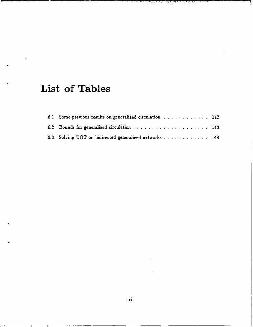
List of Tables
6.1 Some previous results on generalized circulation ............... 142
6.2 Bounds for generalized circulation ..... .................... 143
6.3 Solving UGT on bidirected generalized networks ............... 148
3i
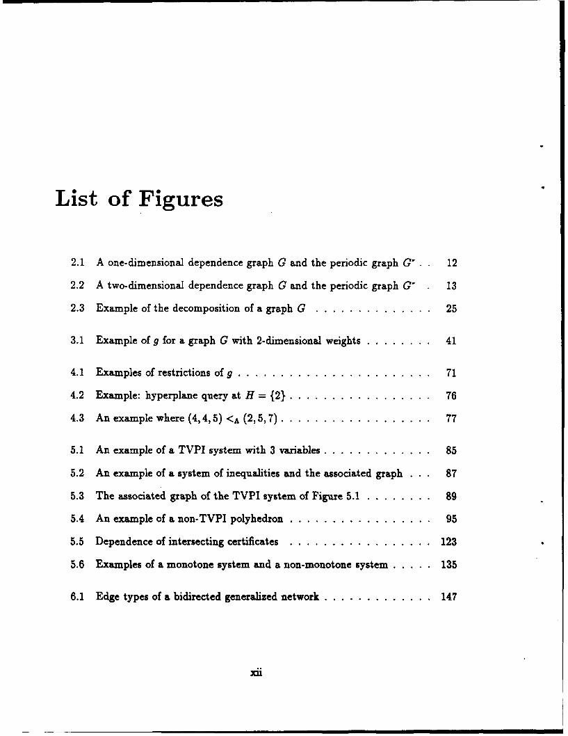
List of Figures
2.1 A one-dimensional dependence graph G and the periodic graph G' . 12
2.2 A two-dimensional dependence graph G and the periodic graph G- 13
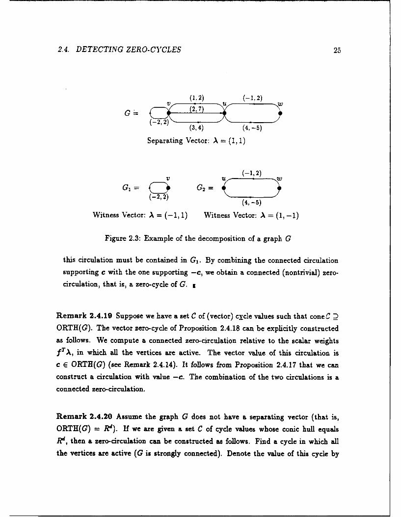
2.3 Example of the decomposition of a graph G .... .............. 25
3.1 Example of g for a graph G with 2-dimensional weights ........ ... 41
4.1 Examples of restrictions of g ...... ....................... 71
4.2 Example: hyperplane query at H = {2}. ...................... 76
4.3 An example where (4,4,5) <A (2,5, 7) ....................... 77
5.1 An example of a TVPI system with 3 variables ................. 85
5.2 An example of a system of inequalities and the associated graph . 87
5.3 The associated graph of the TVPI system of Figure 5.1 .......... 89
5.4 An example of a non-TVPI polyhedron ..................... 95
5.5 Dependence of intersecting certificates .... ................. 123
5.6 Examples of a monotone system and a non-monotone system ..... .135
6.1 Edge types of a bidirected generalized network ................ 147
xii
Chapter 1
Introduction
1.1 Background
Linear programming (LP) is a very widely studied and commonly used class of opti-
mization problems that encompasses many combinatorial optimization problems. A
linear programming problem of n variables and m inequalities consists of a matrix
A E R IXU and two vectors b E Rm, c E R?. The goal is to find a vector: E Rn
(an assignment of values to the variables) such that Ax < b (z satisfies the inequal-
ities) and cT: (the value of the objective function) is maximized. The algorithms
that are most commonly used in practice are variants of the simplex method, due to
Dantzig [16]. None of these variants, however, is known to run in polynomial time
on all instances. The existence of a polynomial-time algorithm for the general LP
problem was in doubt until Khachiyan [40] obtained such an algorithm by modifying
the "ellipsoid method," a tool used in nonlinear optimization. A few years later, Kar-
markar [37] introduced "interior point methods," which hold the promise of yielding
LP algorithms that are both provably polynomial and efficient in practice. Many
others followed (see e.g. [36, 54, 60]). Currently, the best worst-case upper bound for
the problem is due to Vaidya [60].
2 CHAPTER 1. INTRODUCTION
Strongly polynomial algorithms: Vaidya's bound, as well as all known bounds
on the running times of general LP algorithms, depends not only on n and m but also
on the size of the entries. An algorithm for a subset of LP problems is strongly poly-
nomial (SP) if (i) the number of arithmetic operations is bounded by a polynomial
in m and n and (ii) the algorithm does not generate numbers whose size (binary rep-
resentation) is larger than some polynomial function of the input size. An important
open problem is whether general LP has an SP algorithm.
Asymptotic notation: We use the standard asymptotic notation to measure and
compare the resource use (running time, space, processors) of algorithms. Suppose 9
is a monotone increasing function into the positive reals and f is a positive function
defined on the same domain as g. f = O(g) (resp., f = o(g), f = Ql(g), f = w(g),
f = 8(g)) if 3c > 0 such that l"mf/g < c (resp., imf/g = 0, f/g > c infinitely
often, limf /g = oo, f = O(g) and f = 11(g)). We also use the "soft bound" notation
0(f) = O(f polylog f). The common notation for the class of problems solvable in
polynomial time is 7.
Randomized Algorithms: Randomized algorithms make decisions according to
the outcomes of flipping fair coins. Two types of randomized algorithms are men-
tioned in the literature, Monte Carlo algorithms and Las Vegas algorithms. An
asymptotic running time of 0(f) is interpreted as follows: (i) Deterministic algo-
rithms are guaranteed to terminate in 0(f) time. (ii) Monte Carlo algorithms are
guaranteed to terminate in 0(f) time and give an answer that is correct with some
constant probability p > 2/3. (iii) Las Vegas algorithms terminate in 0(f) expected
time and are guaranteed to return a correct answer. The randomized algorithms
discussed in this thesis are Las Vegas type.
Parallel Algorithms: Within the class P, we want to identify problems for which
we can benefit by using a parallel computer, where many processors are available and
able to work concurrently. The PRAM (parallel random access machine) [24] is the
abstract parallel machine model that takes the role played by the Turing machine
1.1. BACKGROUND 3
or RAM in sequential computation. The PRAM is a shared memory multiprocessor
machine. Several types of PRAM'S are considered in the literature, according to
whether they allow concurrent read and write operations from or to the same memory
location. The CREW model, for example, allows concurrent reads but only exclusive
writes. The CRCW model allows both concurrent reads and concurrent writes. A
parallel implementation of a particular algorithm has optimal speedup if the product of
processors and time is of the order of the sequential running time. A complexity class
that somewhat captures the notion of efficient parallel computation is AC. The class
ArC was introduced by Pippenger [53] and is robust in the sense that it applies to many
parallel machine models. A problem is in NVC if it can be solved in polylogarithmic
time using a polynomial number of processors. Obviously, NrC C 'P. A fundamental
open problem is whether 'P = MC. A problem is P-complete if the existence of an AC
algorithm for it implies P = MC, or equivalently, if every problem in 'P can be reduced
to it using logarithmic space. 'P-complete problems are the "hardest" problems in
P. General LP was shown to be P-complete by Dobkin, Lipton, and Rice [18]. The
common belief is that P # AC. Hence, 'P-complete problems in general, and LP in
particular, are viewed to be inherently sequential.
Examples of classes of LP problems with special structure: When a class of
LP problems with special structure is considered, one might try to find either an SP
(resp., MC) algorithm for this class or an SP (resp., logspace) reduction of general LP
problems to problems of this class (see [10]). Such a reduction asserts that proving
that this class is SP (resp., in ANC) is as hard as proving the same for general LP. In
the thesis we consider LP problems of special structure. We are concerned both with
the quantitative problem of improving the parallel and sequential time bounds and
with the qualitative question of strong polynomiality. We give examples of classes of
LP problems that are "easier" than general LP:
9 The maximum flow problem has an SP algorithm due to Edmonds and Karp [21]
and Dinic [17] (better b unds are given in [28, 52]).
4 CHAPTER 1. INTRODUCTION
" The more general minimum-cost circulation problem was shown by Tardos '58!
to have an SP algorithm (see, e.g., [2, 27' for better bounds).
" Tardos [59] generalized her rmin-cost circulation SP algorithm to LP instances
where the entries in the matrix A are bounded by a polynomial in m - n (b
and c can still be general).
" Megiddo [47] gave a linear time algorithm for LP problems with a fixed number
of variables.
" Megiddo [46] gave an SP algorithm for solving linear systems with at most two
variables per inequality. Faster sequential and parallel algorithms are presented
in Chapter 5.
Generalized circulation (see [42]) is an interesting network flow problem. It is not
known to have an SP algorithm and there is no known SP reduction of general LP
problems to it. We present some partial results in Chapter 6.
1.2 Outline of the thesis
The results included in the thesis are joint work with Nimrod Megiddo. The thesis
contains two disjoint sets of results. The first set consists of Chapters 2, 3, and 4
(an extended abstract appeared in [6], see also [7, 91). The second set consists of
Chapters 5 and 6 (an extended abstract appeared in [11]). Chapter 7 contains a
conclusion. Each chapter is more or less independent of the other chapters.
In Chapter 2 we present an algorithm to detect the existence of directed cycles in
periodic graphs. A d-dimensional periodic graph is an infinite digraph, where isomor-
phic finite sets of vertices are associated with the points of the d-dimensional grid.
Periodic graphs have a very regular structure; the edges are such that the periodic
graph "looks the same" from any grid point. A periodic graph can be represented
by a finite directed graph where d-dimensional integer vectors are associated with
the edges. When resolving graph properties of a periodic graph, we would like to
1.2. OUTLINE OF THE THESIS 5
find algorithms whose running time is polynomial in the size of the directed graph
representing it. Periodic graphs in general, and the cycle detection problem in partic-
ular, were studied in previous papers [34, 39, 41, 51]. Previous algorithms, however,
solved the problem by reducing it to polynomially many LP problems (see [39, 41]).
These results left open the existence of strongly polynomial or NVC algorithms for the
problem. The algorithm presented in Chapter 2 is a strongly polynomial and ArC
algorithm, when the dimension d is fixed. To complement the result we also show
that when d is part of the input, the existence of a strongly polynomial time or .'C
algorithm for the problem implies the existence of such an algorithm for general LP
problems. We also show how the same algorithm can be applied to compute strongly
connected components of periodic graphs and to schedule the computation of systems
of uniform recurrences.
The cycle detection algorithm is based on reducing the pi-blem to solving in-
stances of the parametric minimum cycle problem with d parameters. The latter
problem, which is interesting in its own right, can be solved by a sequence of LP
problems. In Chapter 3 we present a method that allows us to perform the com-
putation in SP time and in ANC. The parametric minimum cycle problem is defined
as follows. Consider a digraph where weights are associated with the edges. The
weights are linear functions of d variables ("parameters"). Each set of values for the
parameters corresponds to a set of scalar weights associated with the edges of the
graph. The goal is, roughly, to find the set of values for which the weight of the
minimum-weight cycle is maximized.
The purpose of Chapter 4 is to present the algorithm of Chapter 3 as a general
method to achieve strongly polynomial bounds. The scheme used to maximize the
function that maps sets of parameter values to the value of the minimum-weight
cycle can actually be applied to minimize (resp., maximize) large family of convex
(resp., concave) functions. The minimization requires a number of operations that is
polynomial in the number of operations needed to evaluate the function (when the
dimension of the domain is fixed). In Chapter 4 we omit many of the details specific
to the parametric minimum cycle problem. To allow for independent reading many
definitions and statements are repeated. For some of the proofs, however, the reader
6 CHAPTER 1. INTRODUCTION
is referred to the appropriate place in Chapter 3.
In Chapter 5 we present faster algorithms to solve linear systems of inequalities
where at most two variables appear in each inequality (TVPI systems). We give a
deterministic O(mn2 ) time algorithm and a randomized O(n' + inn) expected time
algorithm, where m is the number of inequalities and n is the number of variables.
In parallel, these algorithms run in 0(n) time with optimal speedup. The previously
best known algorithm due to Megiddo runs in O(mns log in) time sequentially, and
O(n3 log m) time with optimal speedup in parallel [46].
Chapter 6 is concerned with generalized network flow problems. In a generalized
network, each edge e = (u,v) has a positive "flow multiplier" a. associated with it.
The interpretation is that if a flow of x, enters the edge at node u, then a flow of a.z.
exits the edge at v. We present algorithms for generalized network flow problems that
utilize the results of Chapter 5.
The uncapacitated generalized transshipment problem (UGT) is defined on a gen-
eralized network where demands and supplies (real numbers) are associated with the
vertices and costs (real numbers) are associated with the edges. The goal is to find
a flow such that the excess or deficit at each vertex equals the desired value of the
supply or demand, and the sum over the edges of the product of the cost and the flow
is minimized. Adler and Cosares [1] reduced the restricted uncapacitated generalized
transshipment problem, where only demand nodes are present, to solving a single
TVPI system. Therefore, the algorithms of Chapter 5.1.1 result in a faster algorithm
for restricted UGT.
Generalized circulation is defined on a generalized network with demands at the
nodes and capacity constraints on the edges (i.e., upper bounds on the amount of
flow). The goal is to find a flow such that the flow excesses at the nodes are propor-
tional to the demands and maximized. We present a new algorithm that solves the
capacitated generalized flow problem by iteratively solving instances of UGT. The
algorithm can be used to find an optimal flow or an apprbximation. When used to
find a constant factor approximation, the algorithm yields a bound that is not only
more efficient than previous algorithms but also SP. This is the first SP approximation
1.3. NOTATION 7
algorithm for generalized circulation; the existence of this approximation algorithm
is particularly interesting since it is not known whether the problem has an SP algo-
rithm.
1.3 Notation
We use boldface notation for vectors and matrices. Suppose U is a matrix and d is
a column vector, denote by:di - the i'th entry in the vector d,
Uij - the ij entry in the matrix U,
Ui. - the i'th row of the matrix U,
U.j - the j'th column of the matrix U,
UT - the transposed matrix (Vi, j, U, = UT), and
dT - the corresponding row vector.
We use the following special vectors:
e is the vector with all entries 1,
0 is the vector will all entries 0, and
e' is such that e' =1, and for j # i, e 0.
Suppose Ai (1 < i < k) are sets of elements. Denote by:
fAlj the number of elements in the set A. -
Ai x Aj the cross product of A, and A, that is, the set of ordered pairs
(ai, a) where a, E A,, aj E A,.
Xl<i<k- As the cross product of the sets A1 ,... , Ak, that is, the set of k-tuples
(a,,..., a) where ai E A, (1 < i < k).
Af the set of all 1-tuples of elements of Ai.
A nxI the set of all m x n matrices whose entries are elements of Ai.
We use the notation R, R+, Q, Z, and N, for the sets of real numbers, positive
real numbers, rational numbers, integers, and natural numbers, respectively. Hence,
Rk denotes the k-dimensional Euclidean space,Qk denotes the k-dimensional linear space over the rationals, and
Zh denotes the k-dimensional integer grid.
CHAPTER 1. INTRODUCTION
Consider two sets F C Rn and F' C R".
F-F'= {yE R'ly= .- ', where z E F,X'EF'} is thesum ofFand F'.
When every y E F + F' can be uniquely represented as y = x + z' where z E F,
X' E F', we refer to F E F' - F + F' as the direct sum of F and F'.
Denote the projection of F on the coordinates J C {1,..., n} by Fi C R IJ I . Also,
" Fis con-ve'ziffforevery X E F, y E Fand 0 < a < 1, wehaveaz+(l-a)y E F.
" F is a linear subspace iff F = {z E R"hAx = 0} for some matrix A E R' n .
" For a linear subspace F, denote the orthogonal complement of F by F = {z E
Rn Vy E F, zTy = 0}.
" F is a flat iff F = { E R IAx = b} for some matrix A E R" 'XI and vector
b E R m . The subspace parallel to the flat F is {z IAz = 0}.
" F is a cone iff for all X, Y E F and a > 0, 6 0 0, az +RY E F. A cone is
pointed iff it does not contain a linear subspace.
* The lineality space of a cone F is the largest subspace L such that for all z E F,
x+ LcF.
We use the notation:
aff F for the affine hull of F, that is, the smallest flat which contains F,
lin F for the subspace spanned by F,
interior F for the interior of F, and
rel int F for the relative interior (interior relative to aff F).
We denote by g : A --+ B a function from a domain A into B. For a subset
H C A of the domain, denote by gIH the restriction of g to H, that is, the function
gIH : H --+ B such that Va E H, g(a) = gIH(a).
A function g : R' --+ R is convez (resp., concave) if for all z E Rn, y E R, and
0 < z < 1, g(az + (1 - a)y) _< ag(x) + (1 - a)g(y) (resp., g(az + (1 - a) _
ag(z) + (1 - a)g(y)).
1.3. NOTATION 9
By C = (I** E) we denote a directed graph, where V is the set of vertices and E
is the set of edges. We use the convention V! = n, ;E m. By G = (V E. f) we
denote a directed graph with a "weight" function f : E which associates weights with
the edges. For a vertex v E V, let in(v) C " and out(v) C V, respectively, denote
the sets of edges entering and leaving v.
Suppose xT = (xi,..., ,,) are indeterminate.
0 g(X1 .... , zX) is a linear function if there exist real numbers co,..., cn such that
g(XI,. ,) = co - cia
• r' ciXi = co is a linear equation.
* ~ cji= 2 , co and FL', ciai < co are linear inequalities.
" Both linear equations and linear inequalities are referred to as linear constraints.
" A linear system is a set of linear constraints. Set of m inequalities is represented
by a matrix A E Rm Xn and a vector b E R m , as A < b. A vector is feasible if
it satisfies all the constraints.
" A linear programming problem consists of a linear system and a linear objective
function given by a vector c E Rn . The goal is to maximize (or minimize) cTz
subject to the inequalities AZ < b.
Chapter 2
Detecting cycles in periodic
graphs
This chapter is concerned with the problem of recognizing, in a graph with rational
vector-weights associated with the edges, the existence of a cycle whose total weight is
the zero vector. This problem is known to be equivalent to the problem of recognizing
the existence of cycles in periodic (dynamic) graphs and to the validity of systems
of recursive formulas. It was previously conjectured that combinatorial algorithms
exist for the cases of two- and three-dimensional vector-weights. This chapter gives
strongly polynomial algorithms for any fixed dimension. Moreover, these algorithms
also establish membership in the class JVC. On the other hand, it is shown that when
the dimension of the weights is not fixed, the problem is equivalent to the general
linear programming problem under strongly polynomial and logspace reductions. The
algorithms discussed here are based on reducing the problem to soiving instances of
the parametric minimum cycle problem. When the dimension of the vector-weights
is fixed, the problem can be solved within the same time bound of solving an instance
of the parametric minimum cycle problem on the same graph. The latter problem is
defined in Chapter 3, where we present A/C and strongly polynomial algorithm for it
when the number of parameters is fixed. Earlier versions of the results presented in
this chapter appeared in [6, 9].
10
2.1. INTRODUCTION 11
2.1 Introduction
This chapter is concerned with the following problem:
Problem 2.1.1 Given is a digraph G = (I, E, f) where f : E -- Rd associates
with each edge of G a d-vector of rational numbers. Determine whether G contains
a zero-cycle, i.e., a cycle whose edge vectors sum to the zero vector.
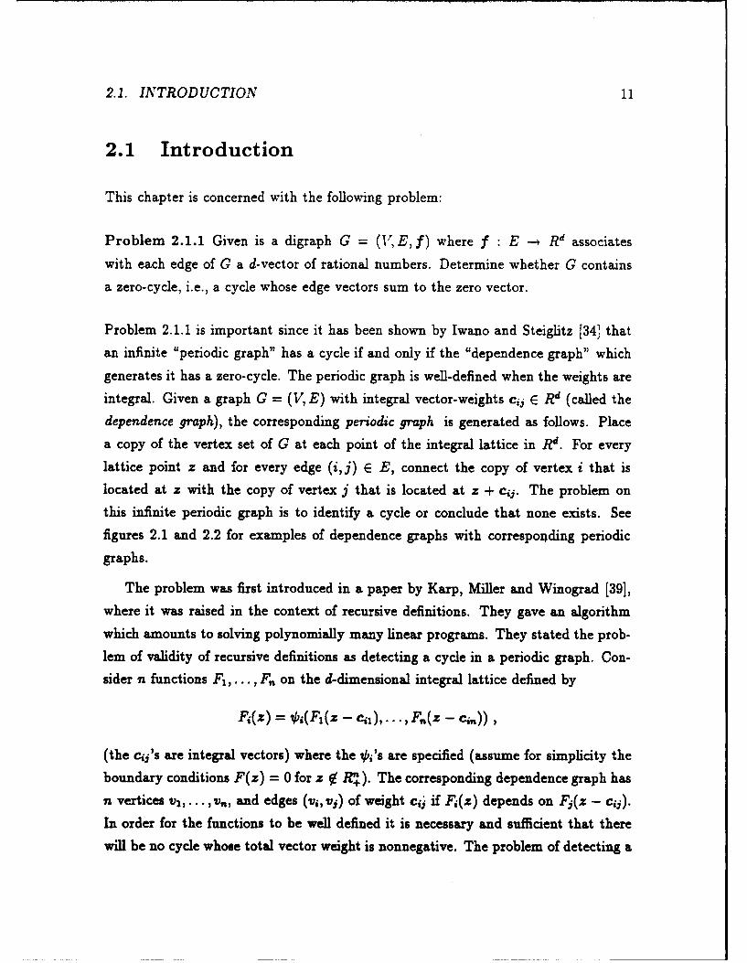
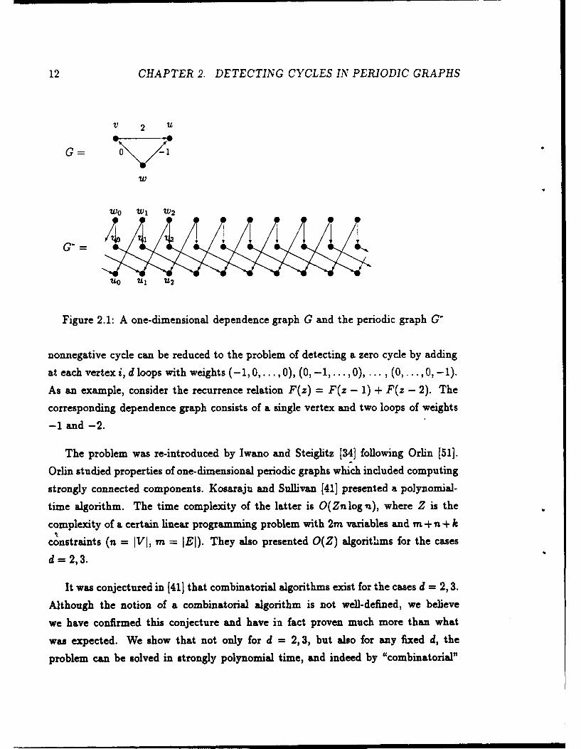
Problem 2.1.1 is important since it has been shown by Iwano and Steiglitz [34] that
an infinite "periodic graph" has a cycle if and only if the "dependence graph" which
generates it has a zero-cycle. The periodic graph is well-defined when the weights are
integral. Given a graph G = (V, E) with integral vector-weights cij E Rd (called the
dependence graph), the corresponding periodic graph is generated as follows. Place
a copy of the vertex set of G at each point of the integral lattice in Rd. For every
lattice point z and for every edge (i, j) E E, connect the copy of vertex i that is
located at z with the copy of vertex j that is located at z + cij. The problem on
this infinite periodic graph is to identify a cycle or conclude that none exists. See
figures 2.1 and 2.2 for examples of dependence graphs with correspotding periodic
graphs.
The problem was first introduced in a paper by Karp, Miller and Winograd [39],
where it was raised in the context of recursive definitions. They gave an algorithm
which amounts to solving polynomially many linear programs. They stated the prob-
lem of validity of recursive definitions as detecting a cycle in a periodic graph. Con-
sider n functions F1,... , F, on the d-dimensional integral lattice defined by
F,(z) = ',0(Fi(z - ci1),.. ., F,(z - cm.)) ,
(the c,'s are integral vectors) where the 0&i's are specified (assume for simplicity the
boundary conditions F(z) = 0 for z V R +). The corresponding dependence graph has
n vertices v2,...,v,, and edges (vi,vj) of weight c., if F(z) depends on Fj(z -cii).
In order for the functions to be well defined it is necessary and sufficient that there
will be no cycle whose total vector weight is nonnegative. The problem of detecting a
12 CHAPTER 2. DETECTING CYCLES IN PERIODIC GRAPHS
V 2 U
G= 0 -1
"WO Wl1 W2 e
11" U1 U12
Figure 2.1: A one-dimensional dependence graph G and the periodic graph G'
nonnegative cycle can be reduced to the problem of detecting a zero cycle by adding
at each vertex i, d loops with weights (- 1, 0,..., 0), (0,-1,..., 0), ... , (0,..., 0,-1).
As an example, consider the recurrence relation F(z) = F(z - 1) + F(z - 2). The
corresponding dependence graph consists of a single vertex and two loops of weights
-1 and -2.
The problem was re-introduced by Iwano and Steiglitz [34] following Orlin [51].
Orlin studied properties of one-dimensional periodic graphs which included computing
strongly connected components. Kosaraju and Sullivan [411 presented a polynomial-
time algorithm. The time complexity of the latter is O(Zn log n), where Z is the
complexity of a certain linear programming problem with 2m variables and m + n + k
constraints (n = JVJ, m = IEI). They also presented O(Z) algorithms for the cases
d= 2,3.
It was conjectured in [41] that combinatorial algorithms exist for the cases d = 2, 3.
Although the notion of a combinatorial algorithm is not well-defined, we believe
we have confirmed this conjecture and have in fact proven much more than what
was expected. We show that not only for d = 2,3, but also for any fixed d, the
problem can be solved in strongly polynomial time, and indeed by "combinatorial"
2.1. INTRODUCTION 13
(1,2)
(0.0)
G'=
Figurt ,.2: A .wo-dimensional dependence graph G and the periodic graph G"
algorithms. Furthermort, our algorithms can be implemented on a parallel machine
sc that membership in the class A/C is established for any fixed d. To complement
these results, we also show that the general problem (where d is considered part of the
input) is as hard as the general linear programming problem in a sense as follows. We
show that any linear programming problem can be reduced in strongly polynomial
time and logspace to our problem with general d.
Consider an instance of Problem 2.1.1 where m = IE is the number of edges and
n = [vI is the number of vertices. We show that when d is fixed the problem can be
solved within the following bounds:
i. O(log2 d n + logd m) parallel time on O(n3 + m) processors.
ii. O(m(log2d n + logd M )) sequential time, when m = f1(n3 log n).
iii. O((n3 + M)log 'd n) sequential time, when m = O(n 3 logn) and m = fl(n 2 ).
14 CHAPTER 2. DETECTING CYCLES IN PERIODIC GRAPHS
iv. O(n 3 log2(d-2 )n nmlog2 (d- l) n) sequential time, when M = O(n2 ).
The constant factors hidden in the above bounds are of the order of 0( 3d ). and arise
from the multi-dimensional search algorithm [5, 19, 47]. The dominating factor in
the time complexity arises from solving O(d) instances of the parametric minimum
cycle problem with d - 1 parameters, m edges and n nodes (see Chapter 3).
It is worth mentioning that other properties of periodic graphs were considered in
the literature. The computation of strongly connected components [51, 9] (see Sec-
tion 2.6.2), scheduling the computation of systems of recursive definitions [9, 39, 56]
(see Section 2.6.1), planarity testing [33], computing'connected components, recog-
nizing bipartiteness [12, 35, 51], and computing a minimum average cost spanning
tree [12, 51].
In Section 2.2 we give some necessary definitions. In Section 2.3 we give an
overview of the basic ideas underlying our algorithms. In Section 2.4 we describe a
strongly polynomial algorithm for detecting zero-cycles. This algorithm is stated in
terms of solving instances of a parametric version of the minimum cycle problem. The
latter problem and a strongly polynomial algorithm for it are introduced in Chapter 3.
Section 2.5 contains some necessary geometric lemmas. Section 2.6 discusses two other
problems on periodic graphs for which the cycle detection algorithm is applicable. One
problem is computing the strongly connected components, the other is scheduling the
computation of systems of uniform recurrences which are modeled by periodic graphs.
Concluding remarks are given in Section 2.7.
2.2 Preliminaries
Definition 2.2.1 Given a graph G = (V, E), a circulation x = (xii) ((i,j) E E) is a
solution of the system:
- = 0 (i =
a >O.
2.3. AN OVERVIEW 15
Let E(x) denote the set of active edges, i.e., edges (i,j) with xij > 0. Vertices incident
on active edges are said to be active in x. If the active edges form a connected
subgraph of G, then we say that the circulation x is connected. If these edges form a
simple cycle, then we say that x is a simple cycle, and with no ambiguity we continue
to talk about the set of active vertices as a simple cycle.
Remark 2.2.2 Every circulation x is a sum of connected circulations, corresponding
to the decomposition of E(x) into strongly connected components. Moreover, it is
also well known (and easy to see) that every circulation can be represented as a sum
of simple cycles. If a connected circulation x = (xij) consists of rational numbers,
then it is proportional to an integral circulation. A connected integral circulation
can be represented by a cycle (u0 ,uj,...,u, = u0) ((ui-i,ui) E E), not necessarily
simple, where z i is interpreted as the number of times the edge (i, j) is traversed
throughout the cycle. It is easy to construct irrational circulations that cannot be
interpreted this way.
Definition 2.2.3 Given vector weights cij = (c!,,..., ) ((i,j) E E) (i.e., using
the notation of Problem 2.1.1, c, = f(e) where e = (i,j)), a circulation x = (:i,) is
called a zero-circulation if it satisfies the vector equation Ejj cijxij = 0. An integral
connected nontrivial zero-circulation is called a zero-cycle.
2.3 An overview
We first present an informal overview of the basic ideas involved in the zero-cycle
detection algorithm.
Suppose G = (V, E, f) contains a vector zero-cycle C, i.e., the sum of the vector
weights cij around C is equal to the zero vector. Obviously, for any A E Rd, the sum
of the scalar weights \Tc~, around C is zero. It follows that for every A E R, the
weight of the minimum cycle relative to the scalars \Tc~j is nonpositive. In other
words, if there exists a A E Rd such that all the cycles are positive relative to T Acj,
16 CHAPTER 2. DETECTING CYCLES IN PERIODIC GRAPHS
then this A certifies that there are no zero-cycles. On the other hand, it can be
shown that if for every A - 0 there exists a negative cycle, then there exists a vector
zero-cycle.
The observation of the preceding paragraph suggests that one might first attempt
to find a A for which all the cycles are positive relative to the weights Acij. In other
words, we wish to maximize over A the weight of the minimum cycle relative to the
scalar weights ATCij.
This task can be viewed as a parameterized extension of the well-known problem
of detecting the existence of a negative cycle or finding a minimum weight cycle in a
graph with scalar weights. The latter scalar weights problem can be viewed as asking
for an evaluation of a function at a given A, which can be solved by running an all
pairs shortest paths algorithm. The search for A as above can be formulated as an
optimization problem over the A-space, where one seeks to maximize the function of
the minimum weight of any cycle relative to the \TC,;s. However, there is a certain
difficulty with this approach since the minimum is not well-defined when there are
negative cycles. Note that we do not require the cycle to be simple, since the problem
of finding a minimum simple cycle is YAfP-hard. However, we can instead consider
one of the following quantities: (i) the minimum cycle-mean, i.e., the minimum of
the average weight per edge of the cycle, or (ii) the minimum of the total weight of
cycles (not necessarily simple) consisting of at most n edges. It is easy to see that
the sign of the minimum cycle-mean (which is the same as the sign of the quantity
defined in (ii)) distinguishes the following three cases: I. there exists a negative cycle,
II. there exists a zero cycle but no negative cycles, and III. all the cycles are positive.
If an algorithm for either (i) or (ii) of the preceding paragraph is given, which
uses only additions, comparisons and multiplications by constants, then such an al-
gorithm can be "lifted" to solve the optimization problem. Very roughly, the basic
idea (which is explained in [44, 45, 46]) is to run the given algorithm simultaneously
on a continuum of values of A, while repeatedly restricting the set of these values,
until the optimum is found. Another interpretation of the lifted algorithm is that it
operates on linear forms rather than constants. When the lifted algorithm needs to
2.3. AN OVERVIETW 17
compare two linear forms, it first computes a hyperplane which cuts the space into
two halfspaces, such that the outcome of the comparison is uniform throughout each
of them. The algorithm then consults an "oracle" (whose details are given later)
for selecting the correct halfspace, and moves on. The lifted algorithm maintains a
polyhedron P which is the intersection of the correct halfspaces.
As noted above, if a vector X is found such that all the cycles are positive then we
are done. Otherwise, the lifted algorithm concludes that A = 0 is an optimal solution,
i.e., for every A there exists a nonpositive cycle, so the choice of A = 0 maximizes the
weight of a minimum cycle. However, the zero vector itself does not convey enough
information. Nonetheless, the algorithm actually computes a vector A # 0 (called
a separating vector) in the relative interior of the set of optima', along with a "cer-
tificate" of optimality. The certificate consists of vector circulation values cl, ... , C,.
These values span in nonnegative linear combinations a suitable linear space, proving
that there is no direction to move so that the minimum cycle becomes positive. This"certificate" is used to actually find a zero-cycle when the algorithm decides that one
exists. The scalar weights XTCij then induce a decomposition of the graph, where two
vertices are in the same component if they belong to the same scalar zero-cycle. It
is then shown that a vector zero-cycle exists in the given graph if and" only if such a
cycle exists in one of the components. Also, if there is only one component (and the
graph has more than one vertex) then there exists a zero-cycle. These observations
suggest an algorithm which iteratively computes a separating vector, decomposes the
graph accordingly, and works on the components independently. The depth of the
decomposition tree is bounded by the dimension of the weights.
The part we have so far left open is the "oracle" which recognizes the correct
halfspace. It turns out that, as in [47], the oracle can be implemented by recursive
calls to the same algorithm in a lower dimension. This will be explained later in the
chapter.
We have outlined the general framework for establishing the qualitative result of
'There is also the possibility that the zero vector is the only optimal solution, so there is noseparating vector. However, in this case, assuming strong connectivity of the graph, it can be shownthat a zero-cycle exists.
18 CHAPTER 2. DETECTING CYCLES IN PERIODIC GRAPHS
strongly polynomial time bounds for any fixed dimension. However, to get more effi-
cient algorithms and to establish membership in A/C, we perform multi-dimensional
searches as in 45, 19, 47]. By doing so we reduce the number of calls to an "oracle"
algorithm which actually need to be performed, to a polylog in the number of deci-
sions. The design can be viewed as an integration of the techniques of L451 and [47]
(and the further improvements of [5, 19]).
2.4 Detecting zero-cycles
In this section we develop an algorithm which decides the existence of a zero-cycle inthe vector-weighted graph G = (V, E, f), f : E --* Z. If a zero-cycle exists in G, we
find an explicit one. The algorithm introduced in this section uses as a subroutine
the parametric minimum cycle algorithm of Chapter 3.
Proposition 2.4.1 A graph G = (V, E, f) with vector weights (see Problem .1.1)has a zero-cycle (see Definition 2.2.3) if and only if it has a connected zero-circulation.
Proof: Note that if there exists a connected zero-circulation then there exists arational connected one. Hence, there exists an integral connected zero-circulation
which is equivalent to a zero-cycle (see Remark 2.2.2). g *
Definition 2.4.2 Given a vector-weighted graph G = (V, E, f ), we use the following
definitions and notation:
i. Let K denote the cone of vectors A = (A,..., Ad)T for which the scalar-weighted
graph (V, E, If T) has no negative cycles.
ii. A nonzero vector A E relint K (the relative interior of K) is called a separating
vector for G.
iii. A separating vector A for which the scalar-weighted graph (V, E, f TA) has onlypositive cycles is called a witness for G.
2.4. DETECTING ZERO-CYCLES 19
A witness proves the nonexistence of nontrivial zero-circulations. Although for this
purpose the vector does not have to be in rel int K, we add this as a requirement
which is helpful in the recursion.
Remark 2.4.3 The cone K can be described as the projection on the A-space (Rd) of
a cone in Rn+d (the space of (r 1,, 7r,,. A)) which is characterized by the inequalities:
7ri- 7rj + ATCj 0 ((i,j) E E).
Note that the system of inequalities above is the linear programming dual of the
zero-circulation problem.
Definition 2.4.4
i. Given G = (V, E, f), denote by CIRC(G) the set of all circulation values c =
i cijzi (where x = (zij) is a circulation in G).
ii. Given a separating vector A # 0 (i.e., A E relint K), denote by ORTH(G, A)
the set of vectors c E CIRC(G) which are orthogonal to A.
Note that CIRC(G) is a convex polyhedral cone.
Proposition 2.4.5 The set K is precisely the set of veclors A such that ATc > 0 for
all c E CIRC(G).
Proof. For any circulation z and any set of scalars wi,
Dir - w3)zj = 0ij
If the (vector) value of z is c, then
ATc =E(A\Tj)Z,ij
By Remark 2.4.3, if A E X then ATe _> 0. Conversely, if A>c 0 for all c E
CIRC(G), then obviously there are no negative cycles in (V, E, fTA), so A E K. X
20 CHAPTER 2. DETECTING CYCLES IN PERIODIC GRAPHS
Theorem 2.4.6
i. ORTH(G, A) is independent of A, and hence will be denoted by ORTH(G). In
fact, ORTH(G) is the lineality space of CIRC(G). (In case K = {0J, define
ORTH(G) to be the entire Rd.)
ii. ORTH(G) = (lin 1C), that is, the orthogonal complement of the linear subspace
spanned by IC (hence it is a linear subspace).
Proof: The proof is based on a geometric analysis which is given in Section 2.5. a
The zero-cycle detection algorithm partitions the graph recursively into node dis-
joint subgraphs. The tree structure defined by this partitioning process, with sub-
graphs as nodes, is referred to as the decomposition tree of the graph G. In this
partition, the subgraphs are the connected components of a "maximal" (in the sense
of the number of active edges) zero-circulation. This definition implies that a zero-
cycle exists in G if and only if a zero-cycle exists at least in one of the subgraphs which
G is partitioned into. If a subgraph is not partitioned any further, it is a 9eal" of
the decomposition tree, and for this subgraph the algorithm determines the existence
of a zero-cycle directly. In [39] and [41] this partition is computed by solving a set
of linear programming problems in order to decide for each edge whether or not it
is active in any zero-circulation in G. The subgraphs are the connected components
induced by the active edges. In this chapter, the computation of the partition is done
differently by an algorithm that gives strongly polynomial time bounds.
For a given graph G = (V, E, f) the algorithm first tries to find a witness (if a
witness is found a zero-cycle does not exist and we stop). In case a witness does not
exist, a separating vector is computed. The computation of a witness or a separating
vector is done by using the parametric minimum cycle algorithm developed in Chap-
ter 3. The algorithm then proceeds to compute a partition of G using the separating
vector found in the previous step. If the partition has only' ne subgraph, it is shown
that a zero-cycle exists in G; otherwise, the algorithm proceeds recursively on the
subgraphs. Note that a witness or a separating vector can be computed by solving
2.4. DETECTING ZERO-CYCLES 21
linear programming problems. The difficulty is to find a strongly polynomial time
solution.
In the rest of this section we first discuss the two subroutines used by the algorithm
and then proceed to the algorithm itself (Subsection 2.4.3). The first subroutine is
the computation of a witness or a separating vector (Subsection 2.4.1). The second
(Subsection 2.4.2) is the partitioning of the graph when a separating vector is given.
2.4.1 Computing a witness or a separating vector
Problem 2.4.7 Given is a graph G = (V E, f). Find a witness for G (see Def-
inition 2.4.2) if one exists; otherwise, find a separating vector A or conclude that
no such vector exists,2 and provide a collection C of circulations with vector-values
cl,... ,c along with a set of positive numbers cu,...,o1 such that r = O(d),
cone{c 1 ,... ,c'} Q ORTH(G), and aici = 0.
Remark 2.4.8 The collection C is used to compute an explicit zero-cycle if one
exists. It enables us to construct a circulation of any given value c' E ORTH(G).
The decision problem (existence of a zero-cycle) can be solved even if C is not given.
Proposition 2.4.9 Problem 2.4.7 can be solved using-three applications of the para-
metric minimum cycle algorithm on G with d - 1 parameters.
Proof: Deferred to Chapter 3. 1
The following proposition is used for the proof of Proposition 2.4.9.
Proposition 2.4.10 Given vectors cl,...,c' C Rd, and a subspace S C Rd, the
following two conditions are equivalent:
i. For every A V S,
min{fTC,...,ATc} < 0.2Note that X # 0 since 0 E X; a separating vector exists if and only if X # {01.
22 CHAPTER 2. DETECTING CYCLES IN PERIODIC GRAPHS
it. conef c',...,Cr} S .
Proof: The equivalence follows from Farkas' Lemma (see Proposition 2.4.12). First
we assume (i) and show that (ii) is implied. Consider z E S'. If a vector y E Rd is
such that yTz < 0, then obviously y J' S. The latter, combined with (i) gives the
left hand side condition on Farkas' Lemma. Therefore, from the right hand side we
have z E cone{c 1 ,..., c,}.
We show that (ii) implies (i). Assume that z E S- => z E conec 1 ,...,c,}. It
follows from Farkas' Lemma that for all z E S', we have (Vy E Rd)yTz < 0 =>
min{yTci} < 0. Consider a vector A V S. There must exist z E S- such that
zTA < 0 (otherwise, Vz E S±,zT y = 0 in contradiction to A 1 S). We have
zTA < 0. Therefore it follows from the left hand side of Farkas' Lemma that
min{, T cj} < 0. 1
Corollary 2.4.11 Let the vectors c1 ,..., c" be circulation values. If for every vector
A %lin X, min{A c\,...,. TCP} < 0, then cone{c ,..., c} ;? ORTH(G).
Proof: Take S = lin K, and recall from Theorem 2.4.6 part (ii) that ORTH(C) =
(lin X)-. I
Proposition 2.4.12 [Farkas' Lemma [2]] For any vectors z, cj E Rd, = 1,... ,
(Vy E Rd)(yTz < 0 min{yc} < 0) * z E cone(ci).
2.4.2 Computing the partition
After computing a separating vector, the zero-cycle detection algorithm proceeds to
compute a partition of the graph. In this subsection we define this partition, and
discuss some of its properties. We also present the algorithm that computes the
partition when the separating vector is given.
The essence of the following proposition is mentioned in [41].
2.4. DETECTING ZERO-CYCLES 23
Proposition 2.4.13 Let G = (V, E, w) be a scalar-weighted graph with no negative
cycles. Using one application of an all-pairs shortest path algorithm we can findvertex disjoint subgraphs G1,... , Gq of G with the following properties. Edges or
vertices that are not active in any zero-cycle of G are not contained in any of the
Gi 's. Two vertices u and v are in the same Gi if and only if there exists a (scalar)
zero-cycle of G in which both u and v are active.
Proof: Apply an all-pairs shortest path algorithm to compute the distance d.
between all pairs of vertices u, v E V. Two vertices u, v are in the same subgraph
Gi if and only if d, + 4 = 0. If d,. > 0, then v is not a part of a zero-cycle and
does not belong to any Gi.
In order to identify all the edges that participate in some zero-cycle, do the following.
Select arbitrarily some vertex w and use a single-source shortest path algorithm to
compute the distarces 7r,, (v E V) from the vertex w to all other vertices. For every
edge (u, v) define,
6.,E7.- 7r., + d.. > 0.
Determine that (u) v) is an active edge if and only if 6,,. = 0. *
Remark 2.4.14 Each component of the partition of Proposition 2.4.13 contains a
zero-cycle where all the vertices of the component are active. This zero-cycle can be
constructed easily from the shortest paths.
Proposition 2.4.15 Suppose A is a separating vector of G = (V, E, f). Consider
the scalar weights w = fTA\ on the edges of G. Observe that by the definition of
a separating vector, there are no negative cycles in the scalar weighted (V, E, w).
Let Gl,..., G. be the partition of G into subgraphs as defined in Proposition .4.13,
relative to the scalar weights w. Under these conditions, a (vector) zero-cycle ezists
in G if and only if a (vector) zero-cycle exists in one of the GC 's.
Proof: The 'if' part is trivial. For the 'only if' part, suppose z is a (vector)
zero-cycle of G = (V, E, f). Then z is a scalar zero-cycle of (V, E, fTA). By
24 CHAPTER 2. DETECTING CYCLES IN PERIODIC GRAPHS
the definition in Proposition 2.4.13, all the vertices active in x are in the same
component Gi and hence x is a vector zero-cycle of Gi. I
Proposition 2.4.16 If CIRC(G) contains a nontrivial linear subspace then a non-
trivial (vector) zero-circulation exists in G.
Proof: The proof is immediate. I
Proposition 2.4.17 If C = {cl,...,c,} C R t and ai > 0 (i = 1,...,r) are such
that Z=j ctici = 0, then for any v E R', it takes 0(12r) time either to find nonneg-
ative rational constants 01 ,... ,3, such that v = Z)3jci, or to recognize that no such
constants exist.
Proof: Express v as a linear combination of the vectors in C by solving the linear
system of equations v = E ici. This system has I equations and r variables, and
thus can be solved by Gaussian eliminations using O(12r) operations. If -y are
nonnegative take 8i = yi; otherwise, denote a = min, <i<, aj, y = min,<i<, -iy and
let 3i = -y - ('y/a)ai. It is easy to verify that #i (1 < i < r) are nonnegative andM-1a Rici = 0. 1
Proposition 2.4.18 Let A be a separating vector of G = (V E, f). Let Gl,... ,G
be the partition of G into subgraphs (as defined in Proposition 2.4.13), relative to the
scalar weights fTA. If the partition constitutes a single subgraph (i.e, q = 1), then G
has a (vector) zero-cycle.
Proof: If G has a single component relative to fTA, then all active vertices and
edges are contained in G1 . Observe that all cycles with vector value in ORTH(G)
are scalar zero-cycles relative to fT. There exists a scalar zero-cycle in (V, E, fTA)
in which all the vertices of G, are active. Thus, there exists a value c E ORTH(G)
which is attained at a circulation where all the vertices in G, are active, so this
circulation is connected. By Theorem 2.4.6 and Proposition 2.4.16, there exists a
circulation, not necessarily connected, whose value is -c. The active vertices in
2.4. DETECTING ZERO-CYCLES 25
(1.2) (-1,2)
(3,4) (4,-5)
Separating Vector: A = (1, 1)
(-1,2)V Uf , ,W
(-2,2) (,5-(4,:-5)
Witness Vector: A = (-1,) Witness Vector: A = (1, -1)
Figure 2.3: Example of the decomposition of a graph G
this circulation must be contained in G1. By combining the connected circulation
supporting c with the one supporting -c, we obtain a connected (nontrivial) zero-
circulation, that is, a zero-cycle of G. I
Remark 2.4.19 Suppose we have a set C of (vector) cycle values such that cone- D
ORTH(G). The vector zero-cycle of Proposition 2.4.18 can be explicitly constructed
as follows. We compute a connected zero-circulation relative to the scalar weightsfTA, in which all the vertices are active. The vector value of this circulation is
C E ORTH(G) (see Remark 2.4.14). It follows from Proposition 2.4.17 that we can
construct a circulation with value -c. The combination of the two circulations is a
connected zero-circulation.
Remark 2.4.20 Assume the graph G does not have a separating vector (that is,
ORTH(G) = Rd). If we are given a set C of cycle values whose conic hull equals
R", then a zero-circulation can be constructed as follows. Find a cycle in which all
the vertices are active (G is strongly connected). Denote the value of this cycle by
26 CHAPTER 2. DETECTING CYCLES IN PERIODIC GRAPHS
c. It follows from Remark 2.4.14 that we can find a circulation with value -c. The
combination of the two circulations is a (nontrivial) connected zero-circulation.
Remark 2.4.21 Remarks 2.4.19 and 2.4.20 discuss the construction of an explicit
zero-cycle. Observe that if C is of size O(d), then the time complexity of constructin b
a zero-cycle is O(d3 ) (see Proposition 2.4.17).
Proposition 2.4.22 A witness for G exists if and only if G does not have a non-
trivial zero-circulation.
Proof: The proof is immediate. *
2.4.3 The algorithm
Algorithm 2.4.23 [zero-cycle detection]
i. Run an algorithm for Problem 2.4.7 on G (see Proposition 2.4.9). If a witness
for G is found then stop. Otherwise, find a collection C of circulation values such
that cone C D ORTH(G), and either find a separating vector A or conclude that
none exists. In the latter case, conclude that a connected zero-circulation, and
hence a zero-cycle, exist in G (see Remark 2.4.20 for an explicit construction of
the zero-cycle). Otherwise,
ii. Construct the partition of G which is defined in Propositions 2.4.13 and 2.4.15.
If the partition is empty then G does not have a zero-cycle. Otherwise,
iii. If there is only one component (i.e., q = 1), then by Proposition 2.4.18, G =
(V,E, f) has a zero-cycle (see Remark 2.4.19 for how to find the zero-cycle
explicitly).
iv. Run the zero-cycle detection algorithm on G1,... , G.- (recursively). By Propo-
sition 2.4.15, G has a zero-cycle if and only if at least one of Gj,..., G. has
one.
2.4. DETECTING ZERO-CYCLES 27
In the rest of the present section we prove the correctness and analyze the com-
plexity of Algorithm 2.4.23.
Proposition 2.4.24 If G is partitioned into G1 , ... , Gq (see Proposition 2.4.15) and
for some Gi, dim(ORTH(Gi)) = dim(ORTH(G)), then Gi will not be partitioned any
further by the algorithm.
Proof: Since ORTH(Gi) C ORTH(G), equality of dimension implies equality of
the sets, so a separating vector for G is a separating vector for Gi. I
Corollary 2.4.25 Algorithm 2.4.23 terminates after at most d - 1 phases of parti-
tioning.
Proposition 2.4.26 The time complezity of the zero-cycle detection algorithm for a
graph G = (V, E, f) (where f is d-dimensional) is dominated by the complezity of 3d
applications of solving Problem 2.4.7 on G.
Proof: First, observe that the complexity of explicitly constructing a zero-cycle
(see Remark 2.4.21) is dominated by the complexity of the rest of the algorithm.
Consider the recursion tree of Algorithm 2.4.23. The recursion tree corresponds to
the decomposition tree of the graph G. By Corollary 2.4.25 this tree has d levels.
Each level is a phase of partitioning a collection of subgraphs Gi,..., Gq, with
total number of n = lVI vertices. The total computation done at such a phase is
solving Problem 2.4.7 for each subgraph Gi, and then, if needed, partitioning it as
described in Proposition 2.4.13. Observe that the time and processor complexities
of solving Problem 2.4.7 and partitioning all the subgraphs at a certain phase,
are dominated by the complexities of the same computation done on the graph G.
Recall (see Proposition 2.4.13) that a partitioning operation amounts to an all-pairs
shortest path computation. Therefore, the complexity of computing the partition is
dominated by the complexity of solving Problem 2.4.7. It follows that at each level
of the tree, the total complexity of the computation is dominated by the complexity
of solving Problem 2.4.7 on G. I
28 CHAPTER 2. DETECTING CYCLES IN PERIODIC GRAPHS
Theorem 2.4.27 The complexity of the zero-cycle detection algorithm for a graph
G = (V, E, f) (where f is d-dimensional) is essentially dominated by 3d applicationsof the parametric minimum cycle algorithm of Chapter 8, applied to instances with
d - 1 parameters which involve the graph G.
Proof. The proof follows from Propositions 2.4.9 and 2.4.26. *
2.5 Geometric lemmas
In this section we give the necessary lemmas which establish the proof of Theo-rem 2.4.6. The reader is referred to [31] for background.
For any subset C of Rd, denote
C + = (Vu E C)(V TU > 0)}.
Recall that a cone which does not contain a nontrivial linear space is said to be
pointed.
The following proposition states well known facts about cones [30].
Proposition 2.5.1
i. Every cone C is a direct sum, C = L 6) C,, of a linear subspace L (the lineality
space of C) and a pointed cone Cp.
ii. The cone C. is contained in the orthogonal complement of L in lin C.
iii. dim(Cp) = dim(C) - dim(L).
Proposition 2.5.2
i. If L C Rd is a linear subspace, then L+ = L± .
ii. For every cone C we have C + = C+ n L±, where C = L E@ CP as above.
2.5. GEOMETRIC LEMMAS 29
Proof: The proof of part i follows from the fact that if L is a linear subspace and
y E L+, then y Td = 0 for all d E L. Part ii follows from the equality C" = C; .L
and from part i. I
Proposition 2.5.3 If C is a pointed cone, C+ is of full dimension.
Proof: The following claim is a consequence of the duality theorem of linear pro-
gramming. For any finite set of vectors ul,... , ut, if there does not exist a vector
a = (a>,...,a)T > 0, a 0, such that Faui = 0, then there exists a vector
v such that vTu i > 1 i = 1,. . . , r. Thus, if C is a pointed cone (not necessarily
polyhedral), there exists a vector v such that for every unit-vector u E C, vTu > 1.
It follows that v E C+ and there exists a ball B, centered at v, such that for every
WE B and u E C (u:# 0) we have wT u > 0. This implies that B C C+.
Proposition 2.5.4
dim(C) = dim(L).
Proof: It follows from Proposition 2.5.3 that C+ is of full dimension in the space
lin C,. Recall that lin Cp, C L+.The proof follows from Proposition 2.5.2 part ii. I
Proposition 2.5.5 If A E relint(C+), then for oll c E C (c 5 0), ATe > 0.
Proof: From the proof of Proposition 2.5.3 and Proposition 2.5.4 it follows that
there exists a vector v such that for every unit-vector u E Cp, vTu > 1, and for
every to E L, vT w = 0. The set C+ is full dimensional relative to L'. Therefore,
if ATc = 0 for some c E Cp (c # 0), then A V relint C+. I
Let C = CIRC(G) (see Definition 2.4.4). Let L and C. be as in Proposition 2.5.1.
Let K be as in Definition 2.4.2.
Proposition 2.5.6
X=C +
30 CHAPTER 2. DETECTING CYCLES IN PERIODIC GRAPHS
Proof: Timmediate from Proposition 2.4.5. 1
Proposition 2.5.7 For every A E relint(kC), the set ORTH(G,A) is equal to the
linear subspace L.
Proof: It follows from Propositions 2.5.5 and 2.5.6, that if A E relint IC and c E Care orthogonal, then c E L. On the other hand, since IC C L' (see Proposi-
tion 2.5.2), if c E L and A E K, then A T c= 0. 1
2.6 Applications of the zero-cycle detection algo-
rithm
We first introduce some notation for the discussion of periodic graphs (see Section 2.1).
For a given G = (V,E,f) where f: E --+ Zd and V = {1,...,n}, denote by G- =
(V', E-) the infinite periodic graph that is defined by G as explained in Section 2.1.
We refer to G- as a d-dimensional periodic graph. Formally,
V'=ZdxV={(z,i) z Z,i EV } -,
E'= Zd xE = {(z,e) z E Zde E E}.
If e = (i,j) we also identify the edge (z,e) with the pair ((z,i),(z + f(e),j)).
The zero-cycle detection algorithm of Section 2.4 computes the decomposition
tree of an input graph G = (V, E, f) and the separating vectors for all the subgraphs
sitting at the nodes of this tree. Recall that this computation can be performed
by solving polynomially many LP programs. In Section 2.4 we presented strongly
polynomial time solution when the dimension d is fixed. We discuss two problems
which can be solved easily when the decomposition tree and the separating vectors
are given.
2.6. APPLICATIONS OF THE ZERO-CYCLE DETECTION ALGORITHM 31
2.6.1 Scheduling
The first application is the problem of scheduling a system of uniform recurrence
equations. The problem was raised by Karp, Miller and Winograd [391 and algorithms
that solve it were given in [39, 56, 55]. These algorithms are stated in terms of solving
systems of linear inequalities and therefore do not establish strong polynomiality.
We show that the knowledge of the decomposition tree and the separating vectors
enables us to produce an immediate solution. Hence, we obtain strongly polynomial
complexity bounds.
A system of uniform recurrence equations is a finite set of relations among func-tions Fi : Z" -- R (i = 1,.. . ,n),
Fi(z) = 0i(Fi(z - Cil),... ,F,(z - C))
(The definition can be easily extended to accommodate the case where the value of
some F is related directly to more than one value of some Fj.) Such a system can be
modeled by a finite graph G = (V, E, f), where the functions F correspond to the
vertices. It is called the "dependence graph" in [39]. This graph defines a periodic
graph G- whose vertices correspond to the function values Fj(z), (i -- 1, ... , n, z EZd z > 0). The direct dependencies among function values are modeled by the edges
of G' as follows. If e = (i,j) E E and f(e) = a, then the evaluation of F(z) requires
the knowledge of F,(z - a) (and having all the required knowledge is sufficient). For
simplicity, suppose it takes one time unit to evaluate the 0i's, that is, given all the
required knowledge, it takes one time unit to calculate the function value.
For "efficient" parallel evaluation of the function values, one would like to find
large sets of "independent" values, that is, sets of values that can be computed simul-
taneously. Here, two values are independent if there is no directed path in G" between
their corresponding vertices. A set of values is called independent if every two mem-
bers of the set are independent. The problem of finding a maximal independent set of
values is not easy, since the problem of deciding whether there exists a directed path
in G", from (zi, i1) to (z 2 ,i 2) is AfP-Complete, even for one-dimensional periodic
graphs (see [51]).
32 CHAPTER 2. DETECTING CYCLES IN PERIODIC GRAPHS
A subspace Si C I is said to be independent if the values Fi(z) (z E Sj) are in-
dependent. Interestingly, one can compute in polynomial time maximal independent
subspaces [39, 56]. Let 1 = Zd X {i}, i = 1,..., n. A maximal independent subspace
Si gives a partition of Vi into independent "isomorphic" flats S,, (v E Si'), where
S,, = (V,O) + Si = {(v + z,i) I z E S,}.
The algorithm for maximal independent subspaces finds for each i, i = 1,..., n, a
matrix Mi of dimensions (d - dim(S i )) x d, whose rows are linearly independent, and
whose null space is Si. Following [56], the matrix Mi is called the scheduling matrix
of i.
An algorithm that computes the scheduling matrix for the special case where
the decomposition tree of G is of depth one was given in [39]. In this special case,
assuming that G is strongly connected, the scheduling matrix would be the same for
all i. In fact, M = M, = ... = M,, consists of a single vector V E Rd , which is
computed by solving a set of linear programming problems. Obviously, the null space
of v is of dimension d - 1. Any solution of the set of linear programs used in [39] is
in the interior of the set {, I (Vc E OIRC)(,Tc > 0)}. Observe that every such v
is a separating vector (see Definition 2.4.2) for G. Moreover, it is a witness since the
decomposition tree has depth one. A more formal statement follows.
Proposition 2.6.1 Suppose G = (V, E, f) is strongly connected and G" has no cy-
cles. If the decomposition tree of G is of depth one and v is a separating vector (and
hence a witness) for G, then the null space of v is a mazinml independent subspace.
Proof: The null space of v has dimension d - 1. Therefore, if it is independent, it
must be maximal. It remains to show that the null space of v is independent. First,
we claim that for any subspace S, if S n CIRC = {O}, then for all i (i = 1,... , n)
and for all u E S-L, the set {(u + z,i) I z E S} is independent. To prove this
claim, assume to the contrary that for some b # 0 in S and some i, there exists
a directed path in G from (u,i) to (u + b,i). Thus, there is a cycle in G with
vector weight b, which implies b E CIRC, and hence a contradiction. Second, we
claim that the intersection of the null space of any witness v with CIRC is equal to
2.6. APPLICATIONS OF THE ZERO-CYCLE DETECTION ALGORITHM 33
{0}. To prove the second claim, observe that if witness exists, then the cone CIRC
of possible circulation values is pointed. Therefore, since ORTH(G) is the lineality
space of CIRC(G) (see Theorem 2.4.6), we have dim(ORTH(G)) = 0. Observe that
ORTH(G) is the intersection of the null space of any separating vector with CIRC
(see Definition 2.4.4). Assuming the second claim holds, the first claim implies that
S(v) is an independent subspace. This concludes the proof of the proposition. *
Roychowdhury and Kailath [56] generalized the result of [39] and gave an algo-
rithm which computes the scheduling matrices for any dependence graph G, where the
decomposition tree is not necessarily of depth one. In the general case, the scheduling
matrices M (i = 1,..., n) need not be all identical, or even of the same dimension.
Their algorithm first computes the decomposition tree of G, along with the separating
vectors of the subgraphs sitting at the nodes of the decomposition tree. Subsequently,
the algorithm uses these separating vectors to construct the scheduling matrices. The
latter construction is trivial (see Definition 2.6.2 and Proposition 2.6.3).
The algorithm of Roychowdhury and Kailath 156] (like the algorithm for the depth
one case of [39]) is based on solving O(m) sets of linear inequalities and therefore,
does not establish strong polynomiality. Recall that the zero-cycle detection algorithm
computes the decomposition tree of G along with a collection of separating vectors
that correspond to the subgraphs of G sitting at the nodes of the decomposition tree.
Hence, the results obtained here imply that the scheduling matrices can be computed
within the time bounds of the zero-cycle detection algorithm, that is, in A/C and
strongly polynomial time.
When the decomposition tree of G and the separating vectors at its nodes are
given, it is easy to compute the scheduling matrices [56]:
Definition 2.6.2 Let G = (V, E, f) be a dependence graph, where V = f1,..., n}.
Consider the decomposition tree of G, and the separating vectors of the subgraphs
sitting at the nodes of the tree. For each vertex i E V, consider the set of subgraphs
that are sitting in the decomposition tree and of which i is a member. This set of
subgraphs corresponds to a path in the decomposition tree. Define the path of a
vertex i to be the ordered set of subgraphs along this path.
34 CHAPTER 2. DETECTING CYCLES IN PERIODIC GRAPHS
Proposition 4.,.3 For a given dependence graph G = (V E, f), the scheduling ma-
trix M of a vertex i is the matrix whose rows are the separating vectors of the sub-
graphs along the path of i.
2.6.2 Strong connectivity
Another application of the zero-cycle detection algorithm is the following. Given a
dependence graph G = (V, E, f), compute the strongly connected components of G-,
that is, find graphs Gi = (Vi, El, f,) such that the graphs G7 are isomorphic to each
of the strongly connected components of G-. The problem of strong connectivity on
periodic graphs was first raised by Orlin [51]. However, his paper is concerned only
with one-dimensional periodic graphs (i.e., when f : E --+ Z is a scalar function).
Orlin gave an algorithm for the one-dimensional case that does not seem to generalize
to higher dimensions. This is not surprising since the strong connectivity problem is
obviously at least as hard as zero-cycle detection in G: the periodic graph G' does
not have a cycle if and only if it has no nontrivial strongly connected components.
We show that the zero-cycle detection algorithm can be used to compute the strongly
connected components of G'. More specifically, we prove that the strongly connected
components are the connected components of the subgraphs sitting at the leaves of
the decomposition tree.
The relation between the decomposition tree of the dependence graph G and the
strongly connected components of G- is given by the following proposition:
Proposition 2.6.4 The strongly connected components of G' are precisely the con-
nected components of the graphs G", where Gi is any subgraph of G sitting at a leaf
of the decomposition tree of G.
Proof: The proof is immediate from the following two claims:
The first claim is that every strongly connected component of G' must be contained
in some G,. This is obvious since all zero-cycles of G must be contained in one of
the Gi's.
2.7. CONCLUDING REMARKS 35
The second claim is that every connected component of a G- is strongly connected.
It suffices to show that every path (ei, E2,... , el) in Gi is part of a zero-cycle. Since
every ej (j = 1, ... , t) participates in a zero-cycle Ci, the cycle U = I Ci is a zero-cycle
which contains the path. *
Remark 2.6.5 A strongly connected component S C V" of G' is such that if
(a, i), (b, i) E S, then (a + a(a - b), i) E S for any integer a.
It follows from Proposition 2.6.4 that for a given dependence graph G = (1, E, f),we can compute a collection of dependence graphs di (i = 1,... , r), such that the
graphs (Gji) are isomorphic to the strongly connected components of G'. This is
done as follows.
Algorithm 2.6.6 [Strongly connected components of G-]
i. Compute the decomposition tree of G. Denote by G (i = 1,...,r) the sub-
graphs sitting at the leaves of the decomposition tree.
ii. For each G, compute a dependence graph di, such that (Gji) is isomorphic to
each of the the connected components of G!.
Step i of the algorithm involves the computation of the decomposition tree, that is,
the zero-cycle detection algorithm. Step ii involves the computation of the connected
components of the G7's. An algorithm for computing connected components of a
periodic graph is given in [8, 12].
2.7 Concluding remarks
The obvious open question that arises is whether Problem 2.1.1, where the dimension
d is part of the input, can be solved in strongly polynomial time, and whether it is
in the class A.C. It is interesting to note the following:
36 CHAPTER 2. DETECTING CYCLES IN PERIODIC GRAPHS
Proposition 2.7.1 The problem of detecting a zero cycle (Problem 2.1.1) is 1'-complete, and also the general linear programming problem is reducible to it in strongly
polynomial time.
Proof: The general linear programming problem is equivalent (in strongly polyno-
mial time and an .AC reduction) to the problem of solving the following system:
Az=0(S)
where A E R' xn. Consider a network consisting of n parallel edges from vertex a
to vertex t and one edge from t to s. (It is a trivial matter to avoid parallel edges
if this is desired.) Associate with the i'th edge the weight-vector given by the i'th
column of A, and associate with the reverse edge the zero vector. The existence
of a nontrivial zero circulation in this network is equivalent to the existence of a
solution to the given system (S). This establishes our claim. I
In view of Proposition 2.7.1, the questions stated in the beginning of this section
axe equivalent to two famous and difficult open questions.
Recall that we considered zero-cycle which were not necessarily simple. Unfortu-
nately, if simplicity of the cycle is added to the requirements, the problem becomes
A/P-complete. Moreover, even the problem of recognizing whether a graph with
scalar weights has a simple cycle with a total weight of zero is AP-complete. This
follows from the fact that the knapsack problem can be reduced to detecting a simple
zero-cycle in a graph whose edges form a ring, where two consecutive vertices are
connected with two parallel edges.
Chapter 3
Parametric minimum cycle
This chapter is concerned with the parametric extensions of the minimum cycle and
the minimum cycle-mean problems. In this problems, we consider graphs with edge-
weights which are linear functions of d parameters. The goal, roughly, is to find an
assignment of the parameters such that the value of the optimal cycle is maximized.
Recall from Theorem 2.4.27 that Problem 2.1.1 can be solved within the same
time bounds as these parametric extensions. The proof of Proposition 2.4.9, which
establishes this relationship, was deferred to this chapter.
The algorithms presented in this chapter to solve the parametric minimum cy-
cle problem introduce a general method. This method is applicable to parametric
extensions of a large class of problems. More specifically, this method introduces a
combinatorial way to optimize a concave function in fixed dimension, when we are
given a piecewise affine algorithm (see Definition 3.1.2) that computes this function.
The latter is discussed further in Chapter 4.
This chapter is organized as follows. In Section 3.1 we give some definitions
and describe the general setup. We also give the proof of Proposition 2.4.9. In
Section 3.2 we present a simplified algorithm for the parametric minimum cycle-
mean problem. The goal of this presentation is to give the reader a sense of how the
strongly polynomial time bounds are achieved. Details which are not essential for
the qualitative result of strongly polynomial time bounds are avoided. The reader
37
38 CHAPTER 3. PARAMETRIC MINIMUM CYCLE
may skip Section 3.2, since the succeeding sections are independent. In Section 3.3 we
give an algorithm for the problem of parametric minimum cycle with at most n edges.
This section introduces additional ideas whose purpose is to improve the sequential
and parallel time bounds.
3.1 Preliminaries
We start by giving some definitions and notations.
Definition 3.1.1
i. For a finite set C C Rd, denote by Lc : Rd --+ R the lower envelope of the
linear functions that correspond to the vectors in C, Lc(A) = mincec cTA. The
vectors c E C, and interchangeably the linear functions cA are referred to as
pieces of Lc. If for A' E R' and C E C we have CTA' = Lc(A') we say that c is
active at A'.
ii. Suppose H C Rd is a flat, F C Rd is the subspace parallel to it, and C =
{ c1,... ,c,} C Rd is a set of vectors. A balancing combination of C relative to
H is a positive linear combination E:=, aici which is orthogonal to F. If H = Rd
we say that i c = 0 is a balancing combination of C if al,. .. , a, > 0.
Let Ri denote the set of vectors A = (A1,... Ad)T E Rd such that Ad = 6.
Definition 3.1.2 For g : Rd --+ R (g : H -- R where H C Rd is a hyperplane), we
introduce the following definitions and notations:
i. Denote by A, a A (possibly A = 0) the set of vectors A E Rd (A E H) where
g(A) is maximized.
ii. Denote by - K the set of A E Rd (A E H) such that g(X) > 0. Also, denote
by K the set of A E K n" Rd.
3.1. PRELIMINARIES 39
iii. An algorithm that computes the function g is called piecewise affine, if the op-
erations it performs on intermediate values that depend on the input vector arerestricted to additions, multiplications by constants, comparisons, and making
copies.
iv. When g = Lc (C C Rd), we say that g' = Lc, is a weak approzimation of g, if the
pieces of g' comprise a subset of the pieces of g (C' C C) and aff A. = aff A91.The function g' = Lc, is a minimal weak approximation of g, if there is noproper subset C" of C' such that Lc,, is a weak approximation of g.
We assume throughout that the function g : Rd - -- R is concave (sometimes wedenote the range by Ri). We also assume that g is given by a piecewise affine al-
gorithm A that evaluates it at a given point. The parametric minimum cycle andparametric minimum cycle-mean problems are special cases of the following problem.The scheme presented here to solve Problem 3.1.3 for these cases, however, can beapplied to any concave function g as above. This is discussed further in Chapter 4.
Problem 3.1.3 I g(X) > 0 for some A, then output such A; otherwise, find A Erelint A. We sometimes add the following requirement. If g < 0, find a subset C of thepieces of g, such that Lc is a minimal weak approximation of g, and find a balancingcombination of C relative to Rld. We refer to this last task as the "optional" part of
the problem.
Intuitively, the set C certifies that the function g does not exceed its maximum
value. The advantage of considering it is that while the number of pieces of g maybe vary large, the size of a minimal weak approximation is at most 2d.
We discuss Problem 3.1.3 where the function g results from parametric extensionsof the minimum cycle and the minimum cycle-mean problems. In an instance ofa parametric problem with d - 1 parameters, edge weights are generalized to belinear functions of the parameters. For each assignment of values to the parameters(vectors in Re), we get an instance of the nonparametric problem. The function g is
40 CHAPTER 3. PARAMETRIC MINIMUM CYCLE
defined as the mapping from assignments of values to the solution of the corresponding
nonparametric problem.
Let G = (VE,f) be as in Problem 2.1.1. The vector-weights f(e) (e - E) are
interpreted as linear functions of d - 1 variables (parameters):
f(e) = f1 (e)Al + "'" + fd-l(e)Ad-1 - - fd(e)
When A is assigned with specific numerical values, we denote by fTA the resulting
set of scalar weights.
Parametric minimum cycle-mean
Definition 3.1.4 Consider G = (V E, f), where for (i,j) E E, f(i,j) = cii E Rd,
i. For a subset of edges E' C E, denote by f(E') the (d - 1)-variable linear
function (1/1E'j) CEE' f(e).
ii. Denote by g(\) the minimum cycle-mean' relative to the scalar-weights \Tci,.
Problem 3.1.5 [Parametric Minimum Cycle-Mean]
For a given graph G = (V, E, f), if g(A) > 0 for some A, then output one such A;
otherwise, find A E relint A.
Parametric minimum cycle:
Definition 3.1.6 Consider G = (V, E, f), where for e E E, f(e) = C. E Rd,
i. For E' C E, denote by f(E') the (d - 1)-variable linear function EE' f (e).
ii. Let C = C(A) denote a cycle of at most n edges which minimizes the total
scalar weight ATc.. Denote g(_) = f(C)T\.
'The minimum cycke-mean is the minimum, over all simple cycles, of the total weight of a cycledivided by the number of its edges.
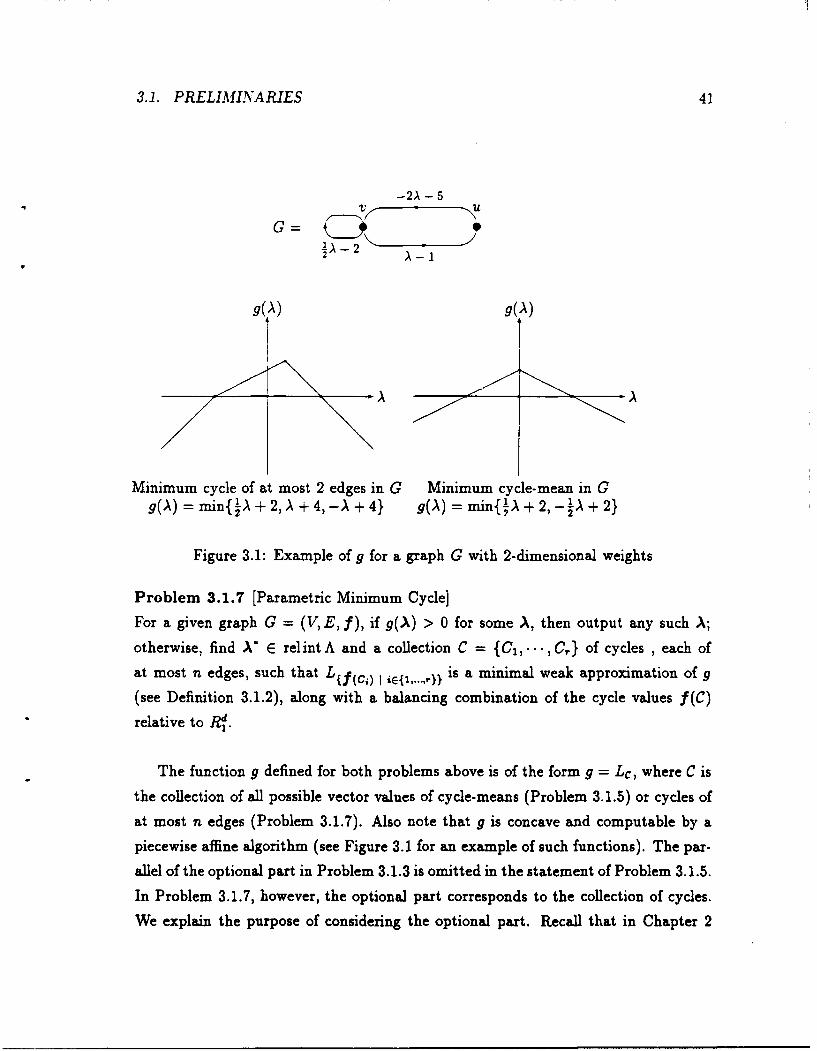
3.1. PRELIMINARIES 41
-2A - 5
G 0- - 2
g(A) g( A)
A -A
Minimum cycle of at most 2 edges in G Minimum cycle-mean in Gg(A) = min{!A + 2, A + 4,-A + 4} g(A) = min{ !A +2, -!A + 2}
Figure 3.1: Example of g for a graph G with 2-dimensional weights
Problem 3.1.7 [Parametric Minimum Cycle]
For a given graph G = (V, E, f), if g(A) > 0 for some A, then output any such A;
otherwise, find A E relint A and a collection C = {C1 , ..- , C,} of cycles , each of
at most n edges, such that L{f(c) I i l ...... 1) is a minimal weak approximation of g
(see Definition 3.1.2), along with a balancing combination of the cycle values f(C)
relative to Rf.
The function g defined for both problems above is of the form g = Lc, where C is
the collection of all possible vector values of cycle-means (Problem 3.1.5) or cycles of
at most n edges (Problem 3.1.7). Also note that g is concave and computable by a
piecewise affine algorithm (see Figure 3.1 for an example of such functions). The par-
allel of the optional part in Problem 3.1.3 is omitted in the statement of Problem 3.1.5.
In Problem 3.1.7, however, the optional part corresponds to the collection of cycles.
We explain the purpose of considering the optional part. Recall that in Chapter 2
42 CHAPTER 3. PARAMETRIC MINIMUM CYCLE
the problem of detecting zero-cycles was reduced to solving Problem 2.4.7. Solving
the latter problem amounts to (i) computing a separating vector, which is needed
to solve the decision problem, and (ii) finding a collection of cycles, which is used
for computing an explicit zero-cycle when one does exist. Proposition 2.4.9 tied the
solution of Problem 2.4.7 to solving instances of the parametric minimum cycle and
the parametric minimum cycle-mean problems. The proof of Proposition 2.4.9 was
deferred to the current chapter. We will see that in order to compute a separating vec-
tor (and hence decide existence of a zero-cycle) it suffices to consider Problems 3.1.5
and 3.1.7 where the optional part is omitted.
The remainder of this section is organized as follows. In Subsection 3.1.1 we define
an important subproblem of Problem 3.1.3. In Subsection 3.1.2 we discuss properties
of weak approximations and balancing combinations. We suggest to skip Subsec-
tion 3.1.2 in first reading. In Subsection 3.1.3 we give the proof of Proposition 2.4.9,
and hence, completing the reduction of the zero-cycle detection problem to solving
instances of Problems 3.1.5 and 3.1.7. The properties given in Subsection 3.1.2 are
used for solving the "optional" part of Problem 3.1.3, that is, to solve the second part
of Problem 2.4.7.
3.1.1 The oracle problem
We find the following subproblem useful for the solution of Problem 3.1.3. The goal of
Problem 3.1.3 is to maximize a function over some domain. Intuitively, the following
is a useful tool: decide on which side of a given query hyperplane (in the A space)
g(A) is either maximized or unbounded. We refer to a procedure that solves this
problem as an oracle. Clearly, such an "oracle" would enable us to perform binary
searches over the A space. In order to achieve strongly polynomial bounds, however,
we use a more sophisticated approach where the number of hyperplane queries needed
is of the order of the number of comparisons done by A. Each hyperplane query can
be resolved by an oracle call. By using the multi-dimensional search techniques and
exploiting the parallelism of A, however, we can do better: We present a solution
where the number of oracle calls performed is a polylog in the number of comparisons
3.1. PRELIMINARIES 43
(hyperplane queries needed).
The function g is a concave piecewise linear mapping from R' into R. Concave
functions have the property that it can be effectively decided which side of a given
hyperplane H contains the maximum of the function. The decision can be made by
considering a neighborhood of the maximum of the function relative to H, searching
for a direction of ascent from that point. This principle is explained in detail in [47]
and is developed below for the special structure of our problem.
Problem 3.1.8 Given is a concave function g: Rd -* R and a hyperplane H in the
A-space.
i. Recognize whether there exists A E H such that g(A) > 0, and if so, output
any such A; otherwise,
ii. find A E H n relint(A), if such a A exists, and generate a solution of Prob-
lem 3.1.3 for g; otherwise, if H n relint A = 0,
iii. recognize which of the two halfspaces determined by H either intersects rel int A,
or has g unbounded on it.
We refer to a procedure that solves Problem 3.1.8 as an oracle and to the hyperplane
H as the query hyperplane.
The method presented here solves instances of Problem 3.1.3 by running a "simula-
tion" of the algorithm A, where (i) additions and multiplication are replaced by vector
operations, and (ii) comparisons are replaced by hyperplane queries. Problem 3.1.8 is
solved by three recursive calls to instances of Problem 3.1.3 on functions of the form
g: -* R. For a point A E RI, define gA = Lc, as the function whose pieces are
all the pieces of g = Lc which are active at A E RI (C' = {c E C I cJA = g(Af)}).The functions to which the recursive calls are made are restrictions of functions of
the form gA to hyperplanes. In Chapter 4 we show that a piecewise afline algorithm
that computes g can be converted to a piecewise affine algorithm that computes g'
and uses the same number of operations. Algorithms that solve Problem 3.1.8 for
44 CHAPTER 3. PARAMETRIC MINIMUM CYCLE
the parametric minimum cycle and the parametric minimum cycle-mean functions
are given later in the current chapter.
3.1.2 Geometric lemmas
We discuss some properties of weak approximations and balancing combinations.
Proposition 3.1.9 Suppose that g = Lc, where C is a finite set of vectors, A' E Ag,
and C' = {c E C I cT\, = g(A)}. The function Lc, is a weak approzimation of g.
Proof: Consider g in a neighborhood of A'. Since C is finite, there exists an open
neighborhood N of A' such that Lc,(A) = g(A) for every A E N. Consider a vector
A' and denote by L the open line segment determined by A' and A'. Consider a point
A" E LfnN, and let C E C' be a piece of g active at A". Since g(A") _< g(A') we have
g(A') < g(A'). Suppose that A' V aff A. We need to show that Lc,(A') < g(A').
For every A E L, g(A) < g(A ), since otherwise we have A' E aff A. In particular
the latter holds for A". It follows that Lc,(A') :_ cIA' < g(A'). I
Corollary 3.1.10 If Lc, is a minimal weak approximation of g, we have cTA = g(A)
for all c E C' and A E a A. It follows that ALe, = aff A.
Proposition 3.1.11 If g = Lc and for some A E relint A and c E C we have
cTA = g(A), then cTA = g(A) for allA E a A.
The proof is immediate.
Proposition 3.1.12 Suppose g = Le, where C C Rd, is bounded from above. Let
C = {ci,. . . ,c,} C C be a set of pieces of g. Under these conditions,
i. The function Lc is a weak approzimation of g if and only if cone C D_ (aff A,)'.
If Lc is a minimal weak approximation of g, coneC = (a A,) 1 .
3.1. PRELIMINARIES 45
it. If Lc is a minimal weak approximation of g, then there exist positive numbers
aC,...c, ? such that E=, a~c1 = 0 and hence hn C = (aff A.)-.
iii. If al,... , at. as in (ii) are given explicitly, then every c E (aff A)- can be ex-
pressed as a nonnegative linear combination of vectors in C using O(d2r) oper-
ations.
Proof: The function Le is bounded from above on Rd, and hence is nonpositive.
Therefore, 0 E A, Le(A) = 0, and aff A = hn A is a subspace. Part (i) follows
from Proposition 2.4.10. The equality when Lc is a minimal weak approximation
follows from Corollary 3.1.10. Parts (ii)-(iii) are direct consequences of Part (i) and
Proposition 2.4.17. 1
Remark 3.1.13 Suppose H = {X E Rd I aT, = 0} (a > 0) is a hyperplane,
F = { E Rd I aT , = 0} is the subspace parallel to H, and A E H is a point on
the hyperplane. By applying standard methods, using 0(d) operations we can find
an affine mapping M from H onto Rd- ' that maps V to 0. All such mappings are of
the form M : H --+ Rd- ', M(A,) = L(,\ - \*) where the matrix L E R(d- 1)xd is such
that L(F) = {L\ I \ E F} = Rd. Within the same time bound we can, compute the
matrices L-1 E R d X(d- 1) which map Rd- ' onto the subspace F, and F E Rdxd such
that for y E Rd, Fy is the projection of V into the subspace F.
Proposition 3.1.14 Let C C Rd be a finite set of vectors, and suppose Lc : Rd
R is bounded. Suppose we are given a hyperplane H C Rd, along with a point
V E AL In. Under these conditions, in O(d3 ) operations we can compute an affine
mapping M H R Rd- ' (M(\') = 0), and a linear mapping of the vectors in
C' = {c E C j cT, = Lc(A)} (the pieces of Lc which are "active" at VX) into vectors
in L C Rd- 1. These mappings convert the problem of computing a minimal weak ap-
proximation of Lc restricted to H into an equivalent problem of computing a minimal
weak approximation of Le R' - ' --* R.
Proof: We use the notation of Remark 3.1.13. It follows from Proposition 3.1.9
that Lc, is a weak approximation of Lc I,, so we can consider only the vectors in
46 CHAPTER 3. PARAMETRIC MINIMUM CYCLE
the set C'. Let K = FL -1 , and C = {Z I c E C'} where E = cTK. We will show
that (i) the set C is such that for all \ E H,c E C', cA = TM(A) + Lc(,\'), and
(ii) for Y C C, the set k C C is such that Lk is a minimal weak approximation of
Le if and only if Ly is a minimal weak approximation of Lc IH.
For a vector y E Rd denote by y' = yTa/!aI the projection of y into the subspace
spanned by a, and denote by Fy = y - y' the projection of y on F. Observe
that F = {,a! 9 E R}-L C Rd, and thus for all XyRd, YE= R +Ty z'y', and
for all A E H we have A' = (\-)'.
For C E C', define 2 = JL- 1 = cK. Consider vectors c E C' and A E H. Recall
that c T,\ = Lc(A'), and therefore we need to show that cT(,\ - \) = ETM(,\).
Note that cT(\- \) = iT(i _ A) + c'(,\,- ()'). Since A' = (A)' for all A C H,
we have cT(,- \) = JL-L(,\ - A') =,ETM(p). I
Proposition 3.1.15 Under the conditions of Proposition 3.1.14 the following holds:
A set of vectors {cl,...,c,} C C', and a set of positive numbers a1 ,.. ,o C4, al > 0
satisfy I -jiE = 0, if and only if E! Ijci = -- /a and -y > 0. Moreover, -y > 0 if
and only if Lc IH < 0. The scalars aj are independent of the particular choice of A'
and the linear mappings.
Proof: We continue to use the notation of the proof of Proposition 3.1.14. Re-
call that ZL = &, and thus E! 1 = (,=i aEi)L = 0. Hence, F,! acj
= Ei a + ac"= aic . Denote c, = cia. We need to show that
,,=2 cgzic _ 0 and the inequality is strict if and only if Lc(A\) < 0. Recall that
for all C E C', cA = Lc(W). Thus, (E:, ac )A" - ,.ac-)a " < 0,
and equality holds if and only if Lc(A') = 0. To conclude the proof, observe that
A' E H, and therefore aTA," = 8 > 0. 1
Proposition 3.1.16 Suppose we are given a set of vectors C = {c,...,c,} C Rd
such that C spans R' and a balancing combination of C (see Definition 3.1.1 part ii).
By using O(rd2 ) operations we can find a minimal subset C' C C 6C'I 2d) that
spans Rd and a balancing combination for C'.
3.1. PRELIMINARIES 47
Proof: Assume that the vectors C1,.... Cd span Rd. In order to find a solution we
use an iterative step with the following properties. If IC - 2d, we find a balancing
combination for C \ C where CC {Cd-,..., C2d+1} and 1( 1. It is easy to verify
that after repeating this step at most r - 2d times, we get a oalancing combination
for a subset C' of C, which spans Rd and is of size at most 2d.
The iterative step is as follows. Solve the linear system of equalities d =
0. The vectors Cd+,... ,C2d- are linearly dependent, and hence this system is
feasible. Assume without loss of generality that for at least one index i, j > 0. Let
I = {d + 1 < i < 2d I Oj> 0}, 12 = {d + 1 < i < 2d Ii <O}, O I= miniE,, (ai/i,
and C = {ci I i E I 1 ,ai//3. = 'y}. We have jiEIuI 2 /3 cic = 0, and C 0 0. Consider
a' = (ak,. .. ,oa) where a = a, (i € I U 12), a = a1 - -y/3i (i E AU 12). It
is easy to verify that ac > 0 and a = 0 if and only if ci E C. It follows that
Ec, c-e ac1 = Ec, c ac - "y 6iUI12 , Ci = 0. Thus, the vectors in C \ C span
R d, and 2cc-e acj is a balancing combination.
The complexity is as follows. The first step amounts to computing d independent
vectors {c1,... ,Cd}, what can be done in O(rd2 ) time. In each iterative step we
solve a system of linear equalities. This can be done in O(d ) operations, using
Gaussian eliminations. Notice, however, that in two consecutive iterations, the
linear systems have d - ICI columns in common. In such a case, when the matrix of
the first problem is given in upper triangular form, the second system can be solved
in only O(Ijd) operations. Thus, the total number of operations is O(rd2 ). I
Corollary 3.1.17 Suppose g = Ly where (Y C Rd) is bounded from above. Assume
we are given a set of vectors C = {cl,... , c,} and a balancing combination of C such
that (i) Lc is a weak approzimation of g, and (ii) there ezist A' E rel int A such that
for all c E C we have eTA" = g(A'). Under these conditions, in O(rd2) operations
we can compute C' C C such that Lc, is a minimal weak approzimation of g, and a
balancing combination of C'. The size of such C' is at most 2(d - dim(A)).
Proof: It follows from Corollary 3.1.10 and Propositions 3.1.11 that for all c E C,
C E (aff A)-. It follows from Proposition 3.1.12 that the vectors C span the subspace
48 CHAPTER 3. PARAMETRIC MINIMUM CYCLE
(affA)'. To conclude the proof, note that the subspace (aff A)"' is of dimension
d- dim(A). m
Proposition 3.1.18 Suppose g = Lc has the property that there exist a vector X' E
relint A such that cTA" = g(A) for all c E C. Suppose we are given:
i. Hyperplanes H6 (6 E {-1,0,1}), where H6 = { I aTA = a + 6} for some
vector a and a E R, and Ha contains A".
ii. Sets of vectors C6 {c,. . } C C and a 6 E Rp (6 {-1,0, 1}) such that
Lc, is a minimal weak approximation of gIH6 , and F,'acs is a balancing
combination of C6 relative to H6 (b E {- 1, O, 1}).
By using O(d3 6E{_1,o01)r6) operations we can compute a set of vectors C and a
balancing combination of C relative to RI, such that C C U6,E-l,o,l) C6 and Le is a
minimal weak approximation of g.
Proof. We give a description of an algorithm. In the first step the algorithm
computes a set C' C C of size at most Escf-1,o0,1 r6 and a balancing combination of
C', such that Le, is a weak approximation of g. This is done as follows.
i. If A C Ho, then C' = U6E{0,1,-I)C6 is such that Lc, is a weak approximation of g.
To find a balancing combination, the algorithm computes fi > 0 (8 {-1, 0, 1})
such that =6e{-1,O,1} /3 E cif = 0. Otherwise,
ii. H n A 6 0 (for either 6 = 1 or 6 = -1). It turns out that the set C' C6 is
such that Lc, is a weak approximation of g. Hence, the algorithm chooses cri
as the coefficients of a balancing combination.
Assuming that C' is a weak approximation of g the algorithm proceeds as follows.
In case ii, C = C' is obviously a minimal weak approximation of g. In case i it
follows from Corollary 3.1.17 that by using O(d ,6c -_,0,1)ro) operations we can
compute C C C and a balancing combination for C, such that Le is a minimal weak
3.1. PRELIMINARIES 49
approximation of g.
What remains is to prove that Lc, is indeed a weak approximation of g. Denote
by A,6 C H6 the set of maximizers of g restricted to H6 . By using an appropriate
translation of the coordinates, we can transform the problem so that C C Rd-1,
g: Rd- -- R, H6 = {A E R d- I aA = 6}, A = 0, and g(A) = 0. This transfor-
mation preserves the property of a subset being a weak approximation or having
a balancing combination relative to a given flat. A balancing combination in the
transformed problem corresponds to a balancing combination relative to Rd in the
original one. Note that in the transformed problem, 0 E A, so the flat aff A is a
subspace.
Let A E relint A6 . Observe that g is linear, that is, for all a > 0, g(aA) = ag(A).
Thus, in case i A = A0. In case ii consider the intersection of A with the open halls-
pace {A I 6(a TA) > 0}. The set A is convex. Thus, if is not empty, it must contain
a relative interior point of A. The hyperplane H6 is contained in this halfspace and
hence this intersection is not empty, and dim A6 = dim A - 1. Note that 0 0 aft A6.
Thus, the flat aff A, E) {#,A 1 /3 E R} must be contained in aff A. On the other hand
this flat is of the same dimension as aff A and therefore equality holds. Consider
any A' E Rd' 1 such that A' V alt A. In order to prove that Lc, weakly approximates
g we need to show that there exists a c E C' such that cTA < 0.
First, we prove case i. If aTA - 0 then we are done, since A E Ho and Co c C'.
Otherwise, assume without loss of generality that a TAI = 'a > 0. Consider the
vector A = A/#. The vector A lies on the line determined by 0 and A, and is such
that a T. = 1. Since aff A is a flat, if it contains two points on a line, it contains the
whole line. Therefore, 0 E aff A and A' V aff A imply that A f a A. It follows that
there exists a C E C1 such that A c < 0. Finally, observe that A'rc = (/3)Tc < 0.
To prove case ii, define A" to be the vector A" = A' + #A where / = (6 -
aTA')/(aTA). Note that aA" = 6 and thus A" E Hi. Moreover, A" al As,
since otherwise A' E af" A. Thus, there exists a c E C6 such that CTA" < 0. We
have A; E ait A and therefore A" has the same projection on (aft A)' as A'. It follows
50 CHAPTER 3. PARAMETRIC MINIMUM CYCLE
from Proposition 3.1.11 that for all c' E C6, c' E (affA). Hence, cTA ' = ¢TA, < 0
To find a balancing combination, recall from Proposition 3.1.15 that there exist
numbers -yj > 0, -1 < 0 such that E! aY = -y a. Hence, we chooseB=E
Oo = 1. It is easy to verify that
E A96EQ = o.bE{-1,0,1} 1
3.1.3 Back to zero-cycles
We are now ready to give the deferred proof from Chapter 2.
Proof of Proposition 2.4.9: Observe that the weight of a minimum weight cycle
in a graph with the scalar weights acrTf (a > 0) is linear in a. If the graph G has
a witness A then either Ad = 0 or the vector (1/Ad)A\ is a witness as well. Therefore,
we can restrict our search on the A-space to vectors A E Rd where Ad E {-1, 0, 1).
Denote
K= fn{y:Yd=6} (6E{-1,0,1}).
Run the parametric minimum cycle (resp., parametric minimum cycle-mean) al-
gorithm on G as defined in Problem 3.1.7 (resp., Problem 3.1.5) three times with
the following (d - l)-variable linear functions. For 6 = -1, 0, 1, we associate with
the edges the linear functions f T,\ 6 where A6 = (A,. . . , A- 1, 6 ). If a witness
for G exists, it must be found during at least one of the three runs. Otherwise,
the maximum of the function g in each of the three subproblems is nonpositive.
Thus, for all three instances, the corresponding sets. '6 E {-1, 0, 1)) consist of
vectors for which g = 0. The algorithm computes nonzero vectors X; E relint X6,
6 E {-1, 0, 1} (if K6 # 0), along with collections C(V) (of size ICM1)l = 0(d)) of cyclessuch that L{f(c) I cee(n} is a minimal weak approximation of g restricted to the
hyperplane Ad = 6, and ar6 are coefficients of balancing combinations of C6 relative
to Ad = 6. To find the separating vector X we proceed as follows. (i) If K6 # 0 for
3.2. ALGORITHM FOR PARAMETRIC MIN CYCLE-MEAN 51
6 E {-1, 1}, we choose A to be A;, and then
A = A E relint)C6 C rel int I.
(ii) If K-1 = K = 0 and K0 5 {0}, we choose A to be a nonzero vector A E
relint Co, and so
A = A; E rel intKC0 = rel int I .
(iii) The remaining case is K- 1 = KI = 0 and /C0 = {0}. Here we conclude that
IC = {}, so there is no separating vector.
As done in the proof of Proposition 3.1.18, using 0(d3 ) operations, we can find a set
C of cycles and a balancing combination for the cycle values {f(C) I C E C}, such
that the lower envelope of the set of cycle values is a minimal weak approximation
of the function g. To conclude the proof observe that the size of a minimal weak
approximation is at most O(2d) (see Corollary 3.1.17), and that cone C D ORTH(G)
(see Corollary 2.4.11). *
3.2 Algorithm for parametric min cycle-mean
In this subsection we sketch a strongly polynomial time algorithm for the parametric
minimum cycle-mean problem. As mentioned before, this algorithm is simpler than
the parametric minimum cycle algorithm. However, its time bounds are worse. The
purpose of discussing it here is to give the reader some intuition and explain some of
the main ideas behind the strongly polynomial bounds. Thus, only the ideas that are
essential for strongly polynomial time bounds are introduced. Two simplifications
are made. First, lie multi-dimensional search technique is not discussed. It improves
the time complexity, but is not essential for strongly polynomial bounds. The second
simplification is that the algorithm only decides the existence of a zero-cycle. There-
fore, the collection C (see Problem 2.4.7) need not be computed, and it suffices to be
able to compute a witness or a separating vector.
52 CHAPTER 3. PARAMETRIC MINIMUM CYCLE
Remark 3.2.1 The minimum cycle-mean relative to a set of scalar weights can be
found in O(:E. - I[) time by an algorithm due to Karp '38]. With n' parallel proces-
sors, the minimum cycle-mean can be computed in O(log s n) time (see [45]).
Proposition 3.2.2 The value of g(,\) can be described as
g(,) = max min (_, + 7rj _ \Tcij)
Proof: Given A E R', consider the following linear programming problem:
Minimize Z(,\TCl,)Zljij
subject to '(xij - xii) = 0 (i = 1,... ,n)(P)
Exij = 11j3
z>O.
Obviously, (P) has an optimal solution. Now, every feasible solution z of (P) is a
convex combination of feasible solutions o', where E(x') is a simple cycle. Since
E x - = 1, the value of the objective function at each z' is precisely the mean weight
of the cycle determined by o'. Hence (P) has an optimal solution of the form z'.
In other words, the optimal value of (P) is equal to g(A). Consider the dual of (P):
Maximize t(D) ""
subject to ri - 7ri + t <
Our claim follows from the fact that the optimal value of (D) is equal to g(A). *
Corollary 3.2.3 The problem of mazimizing g(A) can be formulated as a linear pro-
gramming problem:
Maximize t
subject to r - 7rj+ \Trj + t < 0.
3.2. ALGORITHM FOR PARAMETRIC MIN CYCLE-MEAN 53
The dual of (P) is the following zero-circulation problem:
Minimize E dijiij
subject to (Xij - j) 0 (i ,... n)ij
Z:c 3 = oz>0.
Where c1, = (c ,, d 1), c, E Qd-i.
Remark 3.2.4 In view of Corollary 3.2.3, the problem of maximizing g(A) can be
solved by an extension of the algorithm for linear programming in fixed dimension [47]
and its improvements [5, 19]. Note that only the dimension of the A-space is fixed,
whereas the number of 7ri's varies. However, we will work recursively on the space of
A's where at the base of the recursion (d = 1) we have a problem of the form of (D),
i.e., a problem with fixed scalar-weights which is equivalent to the usual minimum
cycle-mean problem (with no parameters).
Before discussing the algorithm for Problem 3.1.5 we present the respective "ora-
cle" algorithm.
Problem 3.2.5 Given G = (VE, f) and a hyperplane H in the A-space, solve
Problem 3.1.8 for g relative to H.
Problem 3.2.5 (an oracle call) is solved by recursive calls to an algorithm for
Problem 3.1.5 on input graphs with vector weights of a lower dimension as we argue
below.
Theorem 3.2.6 Problem 3.2.5 can be solved by tktee recursive calls to an algorithm
for Problem 3.1.5 in dimension d - 1. The complezity of the additional computation
is dominated by the calls to Problem 3.1.5.
54 CHAPTER 3. PARAMETRIC MINIMUM CYCLE
Proof: Consider Problem 3.1.5 subject to a TA = a (and A E R'). This is in
fact a (d - 1)-dimensional version of the original problem restricted to H = {A C
RdjaTA = al. If g is unbounded on H, then this fact is detected; otherwise, suppose
A(O) is in the relative interior of the set of maximizers of g(A) subject to A E H.
Suppose we also have corresponding values r°,..., . and to) = g(A(0 )) We wish
to recognize whether A(O) is also a relative interior pc'nt of the set of global maxima
(i.e., relative to Rd). If not, we wish to decide whether for all A' E Rd such that
g(A') > g(A(°)), necessarily aTA\ > a, or whether for all of them aTA' < a; these
are all the possible cases. Let E' denote the set of edges (i,j) such that
_r + -, _(,1T~ = to .
Notice that the subgraph G' of G induced by E' contains all the cycles of G whose
cycle-mean is minimum relatively to the weights (AO)Tc 1 j, and only such cycles. In
order to determine whether A0 is in the relative interior of the global maxima (and
if not determine which side of H contains it), we can consider the behavior of g
on two hyperplanes close to H. These hyperplanes are parallel to H, one on each
side. We consider the local maxima relative to these planes. In order to avoid the
problem of how close to get, we can consider just the pieces of g which are active
at A. This is equivalent to considering only cycles whose cycle-mean is minimum
relative to (A°)TC 1.,, namely, the cycles of the subgraph G° . We now solve two
problems on Go of maximizing t subject to
Tri - Trj + ATcij + t < 0 ((i, j) E E ° ) ,
where in one of the problems we also include the constraint OTA = a - 1, .ad in
the other we include the constraint aTA = a + 1. Both problems can be solved
as (d - 1)-dimensional problems since one of the Ai's can be eliminated. Denote
the optimal values of these problems by t(1) and t (-1 ) . Only one of the optimal
values can be greater than t(° ) . If this is the case, or if one of tl), t(- 1) equals t(° )
and the other is smaller, then the side of the hyperplane that contains rel int A
is determined. Otherwise, if either both are less than, br both are equal to t(° ),
then t(° ) is the global optimal value. The base of the recursion is the 1-dimensional
problem (with no parameters at all). I
3.3. ALGORITHM FOR PARAMETRIC MINIMU.M CYCLE 55
A sketch of the algorithm for Problem 3.1.5 is given below.
Algorithm 3.2.7 Consider a minimum cycle-mean algorithm that uses only com-
parisons, additions, and divisions (multiplications) by scalars as primitive operations.
Define the corresponding lifted algorithm to operate on edge weights that are lin-
ear functions, defined by f(e) (e E E). The lifted algorithm maintains a collection
7 of open halfspaces which is initialized as the empty set. Additions and divisions
by scalars are naturally "lifted" to additions and scalar divisions of linear functions.
Comparisons are more intricate. To "compare" two linear functions, we compute the
hyperplane H such that the result of a comparison is uniform throughout each of the
halfspaces defines by H. We then perform an oracle call on H. If the oracle call did
not result in a global solution, a halfspace h is found (one of the sides of H) which
contains the maxima of g. The result of the comparison is the relation between the
linear functions that holds throughout h. The halfspace h is then added to 7- and
the algorithm continues. If the algorithm terminates and no oracle call resulted in
a solution, a separating vector (or a witness) is found by considering a point in the
intersection of all the open halfspaces in X".
3.3 Algorithm for parametric minimum cycle
This section introduces an algorithm for the parametric minimum cycle problem. This
problem is essentially an instance of Problem 3.1.3 for a particular family of functions.
In Chapter 4 we use the general lines of this algorithm to solve Problem 3.1.3 for any
concave function g given by a piecewise affine algorithm.
We suggest an oracle algorithm which relies on making recursive calls to instances
of Problem 3.1.7, where there are fewer parameters, but the weights are more complex.
In order to facilitate the recursion, the problem is generalized to the extended
parametric minimum cycle problem (EPMC). The algorithm presented here solves
the EPMC problem. Let us start with a definition of this problem.
56 CHAPTER 3. PARAMETRIC MINIMUM CYCLE
Extended parametric minimum cycle. Let G = (V, E, w, f) be a graph with
two sets of vectors associated with the edges, i.e., for every e E E, f(e) E Rd and
w(e) E R1. We identify f(e) with the (d - 1)-dimensional linear function:
f(e) = fi(e)A1 + ..- + fd-l(e)Ad-1 + fd(e)
The weight of an edge e is the (I + 1)-tuple (wi(e), ... ,w(e), f(e)). The definitions
given in 3.1.6 are extended as follows.
Definition 3.3.1 Consider a graph G = (V, E, wf), where for e E E, f(e) = C. E
Rd.
i. A cycle C (not necessarily simple) is called w-minimal if the value w(C) =
.-EC w(e) (where edges are counted as many times as they occur on the cycle)
is minimal relative to the lexicographic order on R1.
ii. Let C = C(\) denote a w-minimal cycle of at most n edges which minimizes
the weight c A7 C . Denote g(\) = f(C)A. Note that the first I coordi-
nates of the vector weight of a minimum cycle (i.e., the values given by w) are
independent of A; g(X) gives only the (I + 1)st coordinate.
Remark 3.3.2 For a graph with vector weights in R1, the minimum, relative to the
lexicographic order, among cycles of length less than or equal to n can be computed
in one application of an all-pairs shortest path algorithm. This takes O(IjEj. Vi)
time sequentially, or O(log2 n) time using In' processors in parallel. Therefore, the
function g(A) can be evaluated by a piecewise affine algorithm (see Definition 3.1.2).
Note that g(A) = Le, where C {f(C)IC is a w-minimal cycle}.
Problem 3.3.3 [Extended Parametric Minimum Cycle]
Given is G = (V, E, w, f) as above. If g(A) > 0 for some A, then output any such
A; otherwise, find A E relint A and a collection C = {C 1 ,. . . ,C,} (r < 2d) of w -
minimal cycles, where each consists of at most n edges, such that the lower envelope
L f (C)lC CC of their cycle values is a minimal weak approximation of g, and find a
balancing combination of the cycle values f(Ci),. . . , f(C,) relative to R1.
3.3. ALGORITHM FOR PARAMETRIC MINIMUM CYCLE 5
The EPMC algorithm presented below performs "oracle" calls. The oracle algo-
rithm recursively solves instances of the EPMC problem on G with sets of vector
weights w': E -* R +' and f: E --+ Rd-1.The dimension of the f weights, which
corresponds to the number of parameters, decreases in the recursive calls. In order
to solve an instance of the parametric minimum cycle problem (Problem 3.1.7), we
start with an instance of EPMC where f gives the vector edge weights and w is a
set of null vectors. At the base of the recursion the weights f are null vectors, and
the problem is reduced to the non-parametric problem of computing minimum cycle
relative to the lexicographic order on d-tuples.
In Subsection 3.3.3 we propose Algorithm 3.3.14 for Problem 3.3.3. The algorithm
executes calls to the oracle problem (Problem 3.1.8) relative to g. An algorithm for
the oracle problem is given in Subsection 3.3.1. A call to the oracle is a costly
operation. Therefore, one wishes to solve many hyperplane queries with a small
number of oracle calls. In Subsection 3.3.2 we discuss the multi-dimensional search
technique (introduced in [47]). By applying it, we are able to reduces the number of
oracle calls performed to a polylog in the number of hyperplane queries.
3.3.1 Hyperplane queries
For a given a hyperplane H of R1 , we wish to solve Problem 3.1.8 for g relative to
H. If H n relint A 0 0, we solve Problem 3.3.3, that is, we find A E relint A, the
collection C, and a balancing combination of C.
Problem 3.3.4 Given is G = (V, E, w, f) and a hyperplane H = {A E Rd I aA = al
in the A-space. Solve Problem 3.1.8 for g relative to H.
Theorem 3.3.5 Problem 3.3.4 can be solved by an algorithm which performs three
calls to instances of Problem 3.3.3 where f is (d - 1)-dimensional. The time com-
plezity of the additional computation is dominated by these calls: It can be done
sequentially in CIEI + D time for some constants C = 0(d) and D = 0(d). In
parallel, it can be done in constant B = 0(d 3 ) time using O(m + n') processors.
58 CHAPTER 3. PARAMETRIC MINIMUM CYCLE
Proof: Consider Problem 3.3.3 subject to aTA = a and A = Rd. This is in fact
a (d - 1)-dimensional version of the original problem restricted to the hyperplane
H = {A E Rd I aTA = a}. If g is unbounded on H, then this fact is detected;
otherwise, suppose A(° ) is in the relative interior of the set of maximizers of g(A)
subject to A E H, and we get the collection CM0 ) and a balancing combination of
C0 ) relative to H. Suppose t( °) = g(A(°)). We wish to recognize whether A(° ) is
also a relative interior point of the set of global maxima (i.e., relative to R ). Ifnot, then we wish to decide whether for all A' E Rd such that g(A') _ g(A(°)),
necessarily aTA" > a, or whether for all of them aTA" < a. These are all the
possible cases. Consider G' = (V, E, w', f), where w' = (W, fTA()). Note that
all the minimum cycles of G' correspond to minimum cycles with value t (°) at A
of G. We solve Problem 3.3.3 twice on G', where in one of the problems we also
include the constraint aTA = a - 1, and in the other we include the constraint
aTA = a + 1. Both problems can be solved as (d - 1)-dimensional problems since
one of the Ai's can be eliminated. Denote the optimal values of these problems
by 09 , the corresponding collections of cycles by C6, and let a6 be coefficients
of a balancing combination of C6 (6 E {-1, 1}). Only one of the optimal values
can be greater than t (° ). If this is the case, or if one of t(1 ), t( -1 ) equals t (o) and the
other is smaller, then the side of the hyperplane that contains relint A is determined.
Otherwise, if either both are less than, or both are equal to t(° ), then t (° ) is the global
optimal value. In the latter case A( ) E relint A. It follows from Proposition 3.1.9
that the pieces of g which are active in a minimal weak approximation have the
value t( o) at A(° ) . Thus, a minimal weak approximation of the function g' (see
Definition 3.3.1) which corresponds to G' is a minimal weak approximation of the"original" g which corresponds to the graph G. The conditions of Proposition 3.1.18
and Corollary 3.1.17 hold for the function g'. Hence, in 0(d") operations we can
construct a minimal weak approximation of g, and find a corresponding balancing
combination. The base of the recursion is the one-dimensional problem (with no
parameters at all) where C consists of a single cycle with minimal value, and the
balancing combination is the value of this cycle. I
3.3. ALGORITHM FOR PARAMETRIC MINIMUM CYCLE 59
3.3.2 Employing multi-dimensional search
The multi-dimensional search problem was defined and used in [47. for solving linear
programming problems in fixed dimension.
Problem 3.3.6 [multi-dimensional search]
Suppose there exists an unknown convex set X C Rd, and an oracle is available
such that for any query hyperplane H in Rd, the oracle tells whether X n H = 0;
if so, then the oracle tells which of the open halfspaces determined by H contains
X. For m given query hyperplanes, determine the location of X relative to each of
the hyperplanes, or find any hyperplane (not necessarily one of the given ones) which
intersects X.
The following theorem was proven in [47]:
Theorem 3.3.7 The solution of Problem 3.3.6 relative to some m/2 of the given hy-
perplanes can be found by using -y -y(d) oracle calls. The additional computation can
be done sequentially in O( y(d)m) time, and on m parallel processors in O('y(d) log m)
time. From [5, 19] y(d) = O(( 5 / 9 )d3 d2 ).
Corollary 3.3.8 Problem 3.3.6 can be solved by using O(-y(d)log m) oracle calls and
O('y(d)m) additional time (see [47]).
Remark 3.3.9 The procedure described in [47] can be parallelized so that the ad-
ditional computation (besides the O(-y(d) log m) oracle calls) is done by m parallel
processors in O(-y(d) log2 m) time.
Definition 3.3.10 We define a partial order on Rd \ {0} as follows. For any pair of
distinct vectors a,, a2 E Rd, denote
H H(ai, a2 )={A\ER :al 2aA}
If g is unbounded on H(al, a2) or if H(ai, a 2)fnrel int A 0 0, then we write a, <>A a2.
Otherwise, g can be unbounded on at most one of the open subspaces determined by
60 CHAPTER 3. PARAMETRIC MINIMUM CYCLE
H, and also relint A can intersect at most one of these open halfspaces. We denote
a, <A a 2 (respectively, a, >A a 2 ) if there exists a A E relint A such that aTA < aTjA
(respectively, aTA > aTA), in which case the same holds for all these A's, or if g is
unbounded on the halfspace determined by the inequality aTA < aTA (respectively,
aT\A < a TA). We also use the notation <p for a similar partial order relative to any
set P.
Problem 3.3.11 Given are finite sets A1,... , A, of nonzero vectors, where Ai
{al,... ,a,,} (aj E Rd) and s = cs,. We wish either to find a minimal element,
with respect to the partial order <A, in each of the sets Aj, or (if we encounter two
incomparable elements) to reduce the problem to a lower dimension. More specifically,
we need to find either one of the following:
i. A collection of closed halfspaces whose intersection P contains relint A, and
indices 1 < mi _< si (i = 1,...,r) such that for every 1 < i < r and every
1 < j 8 s,, j 0 mi, we have a <A ai and ai <p a;.
ii. A hyperplane H such that either g is unbounded on H or H n relint A # 0.
Proposition 3.3.12 Problem 3.3.11 can be solved using 0( 7 (d- 1)log s) oracle calls
plus either
i. 0(y-(d - 1) log' s) parallel time on O(s) processors, or
ii. O((d - 1)slog s) sequential time.
(Where -y(d - 1) is as in Theorem S.S.7.)
Proof: The underlying algorithm is an extension of the multi-dimensional search
procedure for Problem 3.3.6 mentioned in Theorem 3.3.7. Here the set X is ei-
ther rel int A or (if the latter is empty) a domain where the function g is un-
bounded. Thus, the case where X intersects the query hyperplane corresponds
to the case where either g is unbounded on the query hyperplane, or the latter
3.3. ALGORITHM FOR PARAMETRIC MINIMUM CYCLE 61
intersects relint A; the case where X is contained in one of the open halfspaces
corresponds to the case where either relint A is contained in the halfspace, or g is
unbounded on the halfspace (but bounded on the hyperplane). Also, note that the
flat R" on which the multi-dimensional search is dane, is of dimension d - 1.
We first explain how to recognize for a given pair of distinct vectors ai, aj whether
a, <A a 2, a 2 <A a, or a, <>A a 2 . Consider the hyperplane H = H(ai,aj) C RI
(see Definition 3.3.10). Suppose H is the query hyperplane presented to an oracle
which recognizes the location of the set rel int A relative to H (in the sense of Prob-
lem 3.3.4). In particular, if H n relint A - 0, then the oracle discovers this fact
and returns a X E H n relint A. Similarly, if g is unbounded on H, then the oracle
reports this fact and provides a A such that g(A) > 0. In the remaining cases the
oracle reports either a, <A a2 or a 2 <A a,.
The multi-dimensional search algorithm computes, adaptively, O(7 (d- 1) log s) hy-
perplane queries. If any of these hyperplanes either intersects rel int A or has g
unbounded on it, then this fact is reported, and the present problem is considered
solved. Otherwise, each of the hyperplanes determines a closed halfspace such that
the intersection P of all these halfspaces has the following property: either g is un-
bounded on the interior of P, or relint A is nonempty and contained in the interior
of P. Moreover, vectors a,, , are found, such that for every i, a. <p a,for all 1 < j <5 si, j 4 ,mi.
We implement the algorithm as follows. View the dimension d as fixed. It was
shown in [5] and [19] that by using a constant number of oracle calls (which, how-
ever, grows exponentially with the dimension) one can locate X relative to at least
half of the hyperplanes. A similar scheme can be applied here. We apply O(log s)
phases. First, for each i (1 < i < r) we match the members of Ai into si/2 ar-
bitrary pairs. This is done with at most s/2 processors. We then calculate the
corresponding (at most a/2) hyperplanes H(a,a 3 ) (see Definition 3.3.10). In a
constant number -y(d - 1) of oracle calls and O(logs) time we can locate relint A
relative to half of these a/2 hyperplanes; unless one of these hyperplanes turns out
to be a valid output (in the sense of (ii) in Problem 3.3.11). We now drop one
62 CHAPTER 3. PARAMETRIC MINIMUM CYCLE
vector from every pair for which the location relative to relint A has been found.
The same is repeated with the remaining 3s/4 vectors, and so on. Altogether, we
run in O(log s) phases, each of which takes 0(-y(d - 1) log s) time on O(s) proces-
sors, and 0(y(d - 1)) oracle calls. The sequential time bound is 0(-Y(d - 1)s log s)
plus 0(-y(d - 1) log s) oracle calls. In parallel, using O(s) processors, the time is
0(-y(d- 1)log 2 s) plus 0(y(d- 1)logs) oracle calls. 1
3.3.3 Algorithm for extended parametric minimum cycle
The algorithm described below solves Problem 3.3.3. It finds a vector A E rel int A,
unless g(A) > 0 for some A, in which case the algorithm outputs such a A. It also
returns a collection C of tn-minimal cycles such that the lower envelope L{f(c)l ccEC
of the linear functions defined by f(C) is a minimal weak approximation of g. The
number of cycles in C is at most 2d.
Definition 3.3.13 Consider a scalar minimum cycle algorithm, where the only prim-
itive operations on expressions that depend on the edge weights are additions, multi-
plications by scalars, and comparisons. We define the corresponding lifted algorithm
for input graphs of the form G = (V, E, f, to). The weight of an edge e E E on
these input graphs is an (I + l)-tuple (w1(e),. . . ,wi(e),f(e)), where f(e) E Rd is
viewed as a (d - 1)-dimensional linear function and to(e) - (w,(e),. . . ,wi(e)). The
lifted algorithm is an extension of the scalar minimum cycle algorithm that operates
on such (I + 1)-tuples instead of scalars. The extension of the operations of addi-
tion and multiplication by a scalar is straightforward, namely, given tuples (to1 , f 1),
(to 2, f 2 ) their sum is (to + to 2, f + f2), and the multiplication by a scalar a is
(aOi, a!f1 ). Comparisons are made with respect to a lexicographic partial order on
the (I + 1)-tuples. It is only a partial order since in the (I + 1)st coordinate we have
the partial order <A (see Definition 3.3.10). To compare two (I + 1)-tuples (tow1 , f )
and (to 2 , f2), we first compare lexicographically the first I scalar coordinates. If the
comparison is not resolved there, we need to compare the linear functions f, and
f2. For this purpose, the lifted algorithm computes the hyperplane H(f 1 , f2) and
3.3. ALGORITHM FOR PARAMETRIC MINIMUM CYCLE 63
solves Problem 3.3.4 (hyperplane query) relative to H. A set of hyperplane queries
is resolved by performing "oracle" calls (see Subsection 3.3.2). The lifted algorithm
maintains a set 7- of closed halfspaces which initially is empty. The hyperplane query
decides whether or not the vectors are comparable. If they are, it decides whether
f I <A f 2 If fI <>A f 2, then the lifted algorithm halts since an oracle call resulted
in a solution to Problem 3.3.3. Otherwise, the resolved hyperplane query tells us
which of the halfspaces defined by H(f 1 , f 2) (see Definition 3.3.10) contains the set
relint A, so this hyperplane is added to X".
Algorithm 3.3.14 [Extended parametric minimum cycle]
Step 1. Run the lifted minimum cycle algorithm, collecting into 7 all the halfs-
paces resulting from oracle calls where comparisons are resolved. Either some
oracle call resulted in a global solution, or otherwise, the algorithm terminates
normally. Denote by CM the minimum cycle found.
Step 2. Denote by P the intersection of the halfspaces in Ni.
i. Compute A' E relint P. This amounts to a linear programming prob-
lemwith d - 1 variables and I2NI constraints, and hence it can be solved
in O(IHI) sequential time [47]. Note that the size of W is bounded by the
number of oracle calls.
ii. If the function Lf(CjM) is not constant on Rd, that is, not all the coef-
ficients fi(CM),j2(CM),..., fd-i(Cm) equal zero, then g is unbounded.
Otherwise,
iii. consider g(),\) = fd(CM).
* If g(A) > 0, then output A and stop. Otherwise,
* the function Lf(CM) is a weak approximation of g, and P = A. Hence,
A" E relint A. Output A* and C = {CM}.
64 CHAPTER 3. PARAMETRIC MINIMUM CYCLE
3.3.4 Correctness
If an oracle call results in a solution in Step 1 of Algorithm 3.3.14, then correctness
follows by induction on the dimension (see also the discussion under Hyperplane
Queries). We now assume that no oracle call resulted in a solution in Step 1. In this
case, a collection %- of closed halfspaces is obtained. Recall that if an oracle call on
a hyperplane H did not result in a solution then the returned halfspace /h has the
following properties: (i) if the function g is bounded then A C h but A Z H, (ii) if
the function g is unbounded, then it must be bounded on the hyperplane H, and
unbounded on the halfspace h. Let P be the polyhedron P = lh' h. It follows that
if g is bounded then P D A, and if g is unbounded then it must be bounded outside
and on the boundary of P. Note that P must be full dimensional (dim P = d- 1), for
if not then it must be contained in one of the query hyperplanes, which contradicts
the previous statement.
Observe that for all pairs a,, a2 of vectors compared by the lifted minimum cycle
algorithm, one of the following must hold: either a, <A a2 and a, <p a 2, or a2 <A
a, and a2 <p a,. The latter is obvious when we perform an oracle call for each
hyperplane query, and it is easy to see that it still holds when we employ the multi-
dimensional search technique (see Problem 3.3.11 and Proposition 3.3.12) and solve
these hyperplane queries by a smaller number of oracle calls. Thus, the vector value
f(CM) of the minimum cycle found by the algorithm must be such that f(CM) <A
f (C) and hence f(CM) <p f(C) for any tv-minimal cycle C. It follows that g(A) =
f(CM)TA for all A E P. Thus, g is unbounded if and only if f(CM) is not a constant,
and the correctness of step ii follows. To show the correctness of step iii assume that
f (CM) is a constant, and thus g = fd(A) for all A E P. Since P D A we have
P = A. It follows that \" E relint A, aff A - R, and Lf(cM) is a minimal weak
approximation of g.
3.3. ALGORITHM FOR PARAMETRIC MINIMUM CYCLE 65
3.3.5 Complexity
The complexity of the algorithm is related to the number of oracle calls. We would like
to resolve many hyperplane queries by performing only a polylogarithmic number of
oracle calls. Thus, it is advantageous to group together many comparisons that could
be done "in parallel" and employ the multi-dimensional search techniques discussed
in Proposition 3.3.12.
Theorem 3.3.15 Algorithm 3.3.14 can be implemented with complexity as follows
(where m = JEl and n = VIJ).
i. O(log2 d n + logd m) parallel time on O(n3 + m) processors.
ii. O(m(log2d n + logdm)) sequential time, when m = fl(n 3 log n).
iii. O(log 2d n(n' + m)) sequential time, when m = O(n'logn) and m = E2(n').
iv. O(n3 log 2(d-2) n + nmlog2 (d- 1) n) sequential time, when m = O(n 2 ).
Proof: The problem of all-pairs shortest path can be solved in O(log2 n) time using
n processors by the Floyd-Warshall algorithm 113). The algorithm for this problem
runs in O(log n) phases. During the first phase, the minimal among all the parallel
edges is determined for each pair of vertices which are linked with at least one edge.
In general, the minimal value in a set is computed for O(n 2) sets, each with O(n)
elements. More precisely, during phase 1, for each ordered pair (i, j) of vertices we
find dfj, the length of shortest path from i to j consisting of at most 2' edges. We
use the relation de- = nin{dtj, mink{dlk + dj}. To find a minimum cycle, we run
one more phase, where we compute a minimum of the diagonal elements in the dis-
tance matrix. The complexity of this last phase is dominated by the other phases.
Each phase can be implemented in one application of Problem 3.3.11, with s = m
for the first phase, and s = n3 for the remaining O(log n) phases. The complexity
is analyzed in Proposition 3.3.12.
Denote by Td and Rd, respectively, the sequential time complexity and the paral-
lel time complexity with n3 + M processors, of the d-dimensional problem. Recall
66 CHAPTER 3. PARAMETRIC MINIVIMUM CYCLE
from Theorem 3.3.5 and Remark 3.3.9 that the time complexity of one oracle call
is 3Td _, = O(Td-l) on a single processor and 3Rd-i = O(Rd._ ) on O(n3 -m M)
processors. When d = 1, an oracle call can be implemented simply by a scalar
minimum cycle algorithm. We derive recursion formulas for R, and T. The or-
acle calls are executed sequentially. First we derive an expression for the paral-
lel complexity when d = 1. Note that the problem can be solved by employing
n3 processors for O(log 2 n) time plus m processors for O(log m) time. Thus, on
O(n 3 + min{m, mlogm/log 2 n}) processors, we have R1 = O(log 2 n + logim). It
follows that
Rd = O(log3 n + log 2 m + (log2 n + log m)Rd-),
which proves i.
The sequential complexity for d = 1 is T1 = O(min{nm, m + n }). Parts ii-iv of the
proposition follow from the recursion:
Td = o(n'logn -+ m + (log 2 n + log m)T-l).
The above analysis applies only to the complexity of Step 1 of the algorithm. In
Step 2 we compute A E relint P. This is done by solving a linear program with
O(7") equations and O(d) variables. The size of W" is at most the number of oracle
calls performed, that is, I7"I = O(log 2 n+log m). Therefore the complexity of Step 2
is dominated by that of Step 1. 1
Remark 3.3.16 There are hidden constant factors in the complexities stated in The-
orem 3.3.15, which depend on the dimension d. First, there is an extra - ctor of d
on the serial time complexity and the number of parallel processors, since most "op-
erations" are done on vectors in R' and take d time units. Second, there is anO(3d-y(d - 1)) factor on the time complexities. The factor -y(d- 1) = 0((5/9) 3( - 1 ) )
is due to the multi-dimensional search (see Subsection 3.3.2), and the factor of 0 (3d)
is due to the fact that an oracle Call involves three calls to a problem of lower dimen-
sion. It follows that the constant factor in the serial time complexity is O(d3d d.y(d- 1)).
In the parallel case there is a factor of 0(3d-y(d - 1)) for the time complexity, and a
factor of O(d) on the number of processors.
Chapter 4
Convex optimization in fixed
dimension
In Chapter 3 we introduced a technique which enabled us to solve the parametric
minimum cycle problem with a fixed number of parameters in strongly polynomial
time. In the current chapter we present this technique as a general tool. In order to
allow for an independent reading of this chapter, we repeat some of the definitions
and propositions given in Chapter 3. Some proofs are not repeated, however, and
instead we supply the interested reader with appropriate pointers.
Suppose Q C R' is a convex set given as an intersection of k halfspaces, and let
g: Q - R be a concave function that is computable by a piecewise affine algorithm
(i.e., roughly, an algorithm that performs only multiplications by scalars, additions,
and comparisons of intermediate values which depend on the input). Assume that
such an algorithm A is given and the maximal number of operations required by A on
any input (i.e., point in Q) is T. We show that under these assumptions, for any fixed
d, the function g can be maximized in a number of operations polynomial in k and
T. We also present a general framework for parametric extensions of problems where
this technique can be used to obtain strongly polynomial algorithms. Norton, Plotkin,
and Tardos [50] applied a similar scheme and presented additional applications.
67
68 CHAPTER 4. CONVEX OPTIMIZATION IN FIXED DIMENSION
4.1 Introduction
A convez .'ptimization problem is a problem of minimizing a convex function g over
a convex set S C R'. Equivalently, we can consider maximizing a concave function.
We consider the problem of maximizing a concave function, where the dimension
of the space is fixed. We also assume that the function g is given by a piecewise affine
algorithm (see Definition 4.2.2) which evaluates it at any point.
The results of this chapter can be extended easily to the case where the range of g
is R1 for any I > 1. We then define the notions of maximum and concavity of g with
respect to the lexicographic order as follows. We say that a function g: Q C Rd --+ R1
is concave with respect to the lexicographic order <le. if for every a E [0, 1] and
M,3y E Q,
ag(aT) + (1 - a)g(y) _<le g(a + 1 -a)y)
Applications where the range of g is R2 were given in [10].
In Section 4.2 we define the problem. In Section 4.3 we introduce the subproblem
of hyperplane queries, which is essential for the design of our algorithm. In Section 4.4
we discuss the muii .-dimensional search technique which we utilize for improving our
time bounds. In Section 4.5 we introduce the optimization algorithm. In Sections 4.6
and 4.7 we prove the correctness and analyze the time complexity of the algorithm. In
Section 4.8 we discuss applying the technique introduced in Chapters 3 and 4 to obtain
strongly polynomial time algorithms for parametric extensions of other problems.
4.2 Preliminaries
Let Rf denote the set of vectors A = (A1 ,... ,Ad)T E Rd such that Ad = 1. For
A E Rd- ', denote by A E Rl the vector A = (A, 1). For a halfspace F, denote by 9F
the boundary of F, i.e., OF is a hyperplane.
4.2. PRELIMINARIES 69
Definition 4.2.1 For a finite set C C R- 1, denote by Lc : Rd' -+ R the minimum
envelope of the linear functions that correspond to the vectors in C, i.e.,
Lc(A) = min cTA.cEC
Denote by Lc : Rd -* R the function given by
Lc (A) = LC~i
The vectors in C C R ~i are called the pieces of g. For a piece c E C and a vector
0 E Rd such that CT = g(o), we say that c is active at 0.
Definition 4.2.2 For a function g : Q -, R, where Q C Rd:
i. Den, - by A, (or A, for brevity) the set of maximizers of g(A). The set A may
be empty.
ii. An -lgorithm that computes the function g (i.e., for A E Q returns the value
g(A) and otherwise stops or returns an arbitrary value) is called piecewise affine,
if the operations it performs on intermediate values that depend on the input
vector are restricted to additions, multiplications by constants, comparisons,
and copies.
iii. For a piecewise affine algorithm 4, u.note by T(A) and C(A) the maximum
number of operations and the maximum number of comparisons, respectively,
performed by A. We assume that this numbers are finite.
iv. If g = Lc for some C C Rd+1, we say that g' = ic, is a weak approximation of
g, if the set of pieces of g' is a subset of the set of pieces of g (C' C C), and the
affine hulls aft A, and aff A,, are equal. The function g' = Lc, is a minimal weak
approximation of g, if there is no C" C C' such that Lc, is a weak approximation
of g.
Remark 4.2.3 Suppose that A is a piecewise afline algorithm. Consider the compu-
tation tree (i.e., the tree consisting of all possible computation paths) of A. Observe
70 CHAPTER 4. CONVIEX OPTIMIZATION IN FIXED DIMENSION
that all the intermediate values along a computation path, including the final out-
put, can be expressed as linear functions (i.e., are of the form aTJ) of the input
vector. These linear functions can be easily computed and maintained during a sin-
gle execution of the algorithm. These linear functions map the input vectors whose
computation path coincides so far with that same path to the corresponding value.
Moreover, the linear function which corresponds to the final output at a single exe-
cution is a piece Which is active at the input vector.
Remark 4.2.4 Suppose 9 : Q C R d - R is concave and computable by a piecewise
affine algorithm A. It is easy to see that there exists a finite set C C Rd~l such that
g coincides with Lc.
Definition 4.2.5 Suppose Q = F1 n... n Fk, is the intersection of k closed halfspaces
and g : Q -- R, g = -C, is concave and computable by a piecewise affine algorithm.
i. For3 E Rd , denoteQo = n{F E Fi}.
Denote by go Qs C Rd --* R the function whose pieces are all the pieces of g
which are active ati3,
go(A) = minjcT5 J4~ g(1 3)}.CEC
Note that go = Lc, where C' = {c E C I cTf3 - g(/S)}. See Figure 4.1 for an
example. Later, we describe an algorithm for evaluating gp.
ii. For a given sequence of vectors 81 ,..- ,/3 E Rd, denote by . the function
((... (gp )0,).. .)0. Note that . depends on the order of the fi's.
iii. Suppose an 1-dimensional flat S C Rd, is represented as a set of solutions of a
linear system of equations. There exists an affine mapping M from Rt onto S,
which can be computed in O(d3 ) time. Denote Qs - {A E R' I M(A) E Q},
and define gS : QS -. R by gs = g o M.
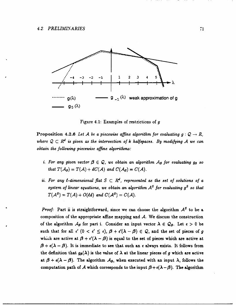
4.2. PRELIMINARIES 71
......... g () g -1 () weak approximation of g
- g 5 (0)
Figure 4.1: Examples of restrictions of g
Proposition 4.2.6 Let A be a piecewise affine algorithm for evaluating g: Q -R,
where Q C Rd is given as the intersection of k halfspaces. By modifying A we can
obtain the following piecewise affine algorithms:
i. For any given vector /3 E Q, we obtain an algorithm AO for evaluating go so
that T(Ap) = T(A) + dW(A) and C(AO) = C(A).
ii. For any f-dimensional flat S C Rd, represented as the set of solutions of a
system of linear equations, we obtain an algorithm As for evaluating gS so that
T(A s ) = T(A) + 0(id) and C(A s ) = C(A).
Proof: Part ii is straightforward, since we can choose the algorithm As to be a
composition of the appropriate affine mapping and A. We discuss the construction
of the algorithm AO for part i. Consider an input vector A E QO. Let e > 0 be
such that for all c' (0 < e' < e), /3 + e'(-\ - /3) E Q, and the set of pieces of g
which are active at /3 + c'(\ - /3) is equal to the set of pieces which are active at
/3 + e(A - /3). It is immediate to see that such an c always exists. It follows from
the definition that go(A) is the value of A at the linear pieces of g which are active
at /3 + c(A - /3). The algorithm AO, when executed with an input A, follows the
computation path of A which corresponds to the input /3 + e(A - /3). The algorithm
72 CHAPTER 4. CONVEX OPTIMIZATION IN FIXED DIMENSION
computes the linear functions associated with the intermediate values of this path
(see Remark 4.2.3). Recall that the linear function which corresponds to the final
value is a piece of g which is active at 83 + E(A - ,3). Hence, the value of gs(A\) is
obtained by substituting A in this linear function. In order to follow the desired run
of A, the algorithm ,6 mimics the work of A on additions and multiplications by
scalars, keeping track of linear functions rather than just numerical values. When
the run of A reaches a comparison (branching point), .Aq does as follows. Without
loss of generalit- we assume that the branching is according to the sign of the
linear function aT:. In order to decide what to do at a branching point, A, has
to determine the sign of a T at the point z = /3 + E(A - 3). Since E is not given
explicitly, the decision cannot be made directly by substitution. The decision is
made as follows. The algorithm first computes a = a T 1. If a 0 0, then obviously
for any vector y, for sufficiently small number E > 0 aT(/3 "+"ey) has the same sign
as a. In particular this holds for y = A -/3 and the sign is detected. Otherwise, if
a = 0, it follows that at(/3 + e(A -/3)) = eaTi. Hence aT5 has the same sign as
aT( + e(A -/3)). It remains to compute the sign of aTi and branch accordingly.
It is easy to verify that Ap evaluates the function gs for any vector A E Q6, and
performs the stated number of operations. I
Proposition 4.2.7 If )9 E A. then go is a weak approzimation of g (see Proposi-
tion 3.1.9 for a proof).
The goal is to solve the following problem:
Problem 4.2.8 The input of this problem consists of a polyhedron Q = ...-- n Fk,
given as the intersection of k closed halfspaces and a piecewise alline algorithm A for
evaluating a concave function 9 : Q -- R. Decide whether or not g is bounded. If
so, then find a A' E relint A. We refer to the following as the "optional" part of the
problem: If g is bounded, then find a subset C of the set of pieces of g, such that Lc
is a minimal weak approximation of g, and IC] < 2d.
The set C may be viewed as a certificate for the fact that the maximum of the
function g does not exceed g(A*). In the current chapter we do not discuss the details
4.2. PRELIMINARIES 73
of solving the optional part of the problem. See Chapter 3 for an existence proof and
an algorithm which finds such a set.
We propose an algorithm for Problem 4.2.8. In any fixed dimension d, the total
number of operations performed by this algorithm is bounded by a polynomial in T(A)
and k. The algorithm is based on solving instances of a subproblem, which we call
hyperplane query: For a given hyperplane H0 , decide on which side of H0 the function
g is either unbounded or attains its maximum. A procedure for hyperplane queries is
called an oracle. Obviously, an oracle can be utilized to perform a binary search over
the polyhedron Q. However, in order to attain an exact solution within time bounds
that depend only on d, T, and k, we use the oracle in a more sophisticated way.
The number of hyperplane queries needed by the algorithm, and hence the number
of oracle calls, is bounded by the number of comparisons performed by A. We later
discuss applying the multi-dimensional search technique, what allows us to do even
better. By exploiting the parallelism of A, the number of oracle calls can in some
cases be reduced to a polylogarithm of the number of hyperplane queries.
The function g is a concave piecewise linear mapping. Concave functions have
the property that it can be effectively decided which side of a given hyperplane Ho
contains the maximum of the function. If the domain of g does not intersect H0, then
the answer is the side of Ho which contains the domain of g. Otherwise, the decision
can be made by considering a neighborhood of the maximum of the function relative
to Ho, searching for a direction of ascent from that point. This principle is explained
in detail in [47].
For a hyperplane H0 C Rd, we wish to decide on which side of Ho the set relint A
lies. By solving a linear program with d variables and k + 1 constraints, we determine
whether or not Ho n Q = 0, and if so, we determine which side of Ho contains Q. It
follows from [47] that this can be done in 0(k) time. If H0 n Q # 0, then the oracle
problem solves the original problem, when g is restricted to Ho. If g is unbounded on
H0 the oracle reveals that. If A = 0, or if relint A is either contained in Ho or extends
into both sides of Ho (i.e., Ho n relint A # 0), then we find A E H0 n relint A and the
oracle will actually solve Problem 4.2.8.
74 CHAPTER 4. CONVEX OPTIMIZATION IN FIXED DIMENSION
Problem 4.2.9 Given are a set Q = F1 n ... 7 Fk, a piecewise affine algorithm A
which evaluates a concave function g Q -- R, and a hyperplane H0 in Rd. Do as
follows:
i. If Q - H0 = 0, recognize which of the two halfspaces determined by H0 contains
Q. Otherwise,
ii. recognize whether or not g is bounded on H0 . If it is, then
iii. find \ E Ho n relint A if such A exists, and solve Problem 4.2.8 relative to g.
Otherwise, if H0 n relint A = 0, then
iv. recognize which of the two halfspaces determined by H0 has either a nonempty
intersection with relint A, or has g unbounded on it.
A procedure for solving Problem 4.2.9 will be called an oracle and the hyperplane H0
will be called the query hyperplane. Problem 4.2.8 is solved by running a modification
of the algorithm A, where additions and multiplications are replaced by vector opera-
tions and comparisons are replaced by hyperplane queries. Problem 4.2.9 is solved by
three recursive calls to instances of Problem 4.2.8 of the form (AH, QH), (Ac, Q'),where ) E Rd, and H is a hyperplane (see Definitions 4.2.5 and 4.2.6). Note that these
algorithms compute, respectively, the functions gH : QH --+ R, g : QH --* R, whereQH and QH are subsets of Rd- '. Hence, the recursive calls ari made to instances of
lower dimension.
In Section 4.5 we propose Algorithm 4.5.2 for Problem 4.2.8. The algorithm
executes calls to the oracle problem (Problem 4.2.9) relative to g. An algorithm for
the oracle problem is given in Section 4.3. A call to the oracle is costly. Therefore,
one wishes to solve many hyperplane queries with a small number of oracle calls. In
Section 4.4 we discuss the multi-dimensional search technique (introduced in [47]).
4.3 Hyperplane queries
For a hyperplane H C Rd, we solve Problem 4.2.9 for g relative to H.
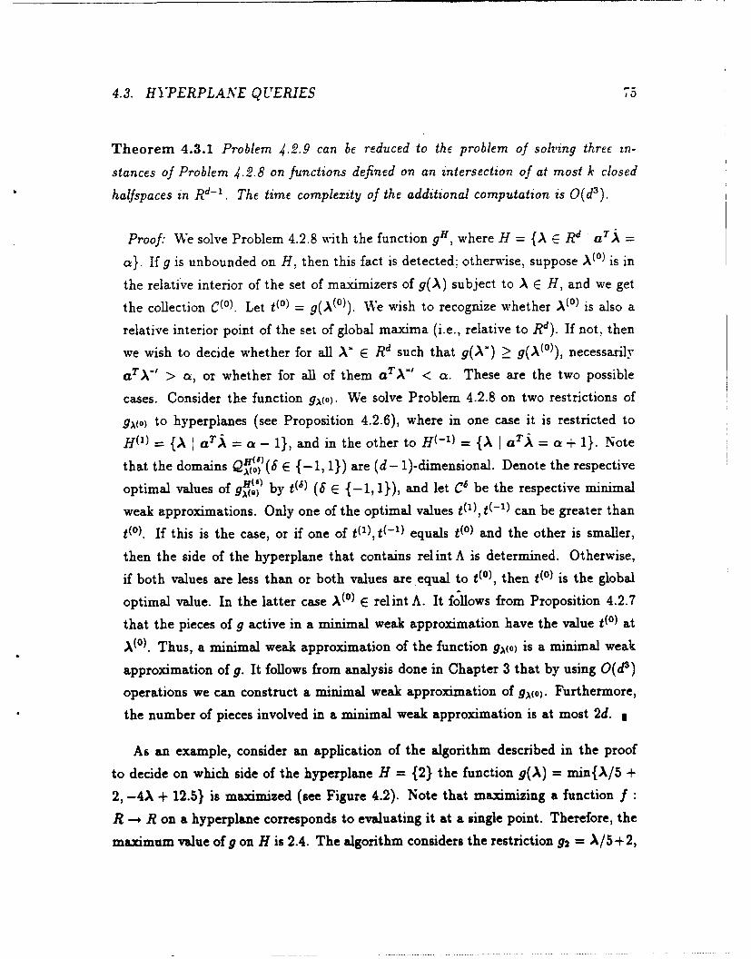
4.3. HYPERPLANE QUERIES 75
Theorem 4.3.1 Problem .4.2.9 can be reduced to the problem of solving three in-
stances of Problem 4.2.8 on functions defined on an intersection of at most k closed
halfspaces in Rd- 1 . The time complexity of the additional computation is 0(d 3 ).
Proof: We solve Problem 4.2.8 with the function gH, where H = {A R d aTli =
a}. If g is unbounded on H, then this fact is detected; otherwise, suppose A(0) is in
the relative interior of the set of maximizers of g(A) subject to A E H, and we get
the collection C(° ). Let t (° ) = g(A(°)). We wish to recognize whether A(° ) is also a
relative interior point of the set of global maxima (i.e., relative to Rd). If not, then
we wish to decide whether for all A E Rd such that g(A') _! g(A(°)), necessarily
aTAkI > a, or whether for all of them aTA' < a. These are the two possible
cases. Consider the function gA(o). We solve Problem 4.2.8 on two restrictions of
g(o) to hyperplanes (see Proposition 4.2.6), where in one case it is restricted to
H (' ) = {A I a = a - 1}, and in the other to H (- ' ) = {A I aTA = a + 1}. Note
that the domains Q'0(6)( E {-1, 1}) are (d- 1)-dimensional. Denote the respective
optimal values of 9H o)) by t (6) (6 {-1, }), and let C6 be the respective minimal
weak approximations. Only one of the optimal values tl ) , t(-' ) can be greater than
t (° ). If this is the case, or if one of t (1), t(- 1) equals t (° ) and the other is smaller,
then the side of the hyperplane that contains relint A is determined. Otherwise,
if both values are less than or both values are equal to t ('), then t(') is the global
optimal value. In the latter case A ° ) E relint A. It follows from Proposition 4.2.7
that the pieces of g active in a minimal weak approximation have the value t (o) at
A(° ). Thus, a minimal weak approximation of the function g0(o) is a minimal weak
approximation of g. It follows from analysis done in Chapter 3 that by using 0(d 3 )
operations we can construct a minimal weak approximation of g\(o). Furthermore,
the number of pieces involved in a minimal weak approximation is at most 2d. I
As an example, consider an application of the algorithm described in the proof
to decide on which side of the hyperplane H = {2} the function g(A) = min{A/5 +
2,-4A + 12.5} is maximized (see Figure 4.2). Note that maximizing a function f :
R --* R on a hyperplane corresponds to evaluating it at a single point. Therefore, the
maximum value of g on H is 2.4. The algorithm considers the restriction g = A/5+2,
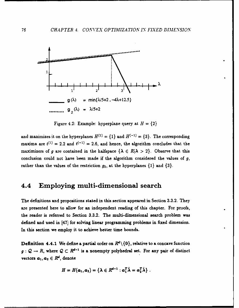
76 CHAPTER 4. CONVEX OPTIMIZATION IN FIXED DIMENSION
.~~ ~ ~ . ... ....... : o........
g (k) = min{5+2,-4,+12.5}
......... g2 (X) = /5+2
Figure 4.2: Example: hyperplane query at H = {2}
and maximizes it on the hyperplanes H(1) = {1} and H (- ' ) = {3}. The corresponding
maxima are t (l) = 2.2 and t( - ') = 2.6, and hence, the algorithm concludes that the
maximizers of g are contained in the halfspace {A E RIA > 2}. Observe that this
conclusion could not have been made if the algorithm considered the values of g,
rather than the values of the restriction 92, at the hyperplanes {1} and {3}.
4.4 Employing multi-dimensional search
The definitions and propositions stated in this section appeared in Section 3.3.2. They
are presented here to allow for an independent reading of this chapter. For proofs,
the reader is referred to Section 3.3.2. The multi-dimensional search problem was
defined and used in [47] for solving linear programming problems in fixed dimension.
In this section we employ it to achieve better time bounds.
Definition 4.4.1 We define a partial order on R" \{0}, relative to a concave function
g : Q --+ R, where Q C R"- ' is a nonempty polyhedral set. For any pair of distinct
vectors al, a 2 E Rd, denote
H=H(al, a2 ) = {A E a~d = 4Aa}.
4.4. EMPLOYING MULTI-DIMENSIONAL SEARCH 77
Y
4y+4x+5 >A2y+5x+7j 4y+4x+5 < 2y+5x+7
x-2 -1
Figure 4.3: An example where (4,4,5) <A (2,5, 7)
If g is unbounded on H(ai, a 2 ) or if H(ai, a 2)flrelint A # 0, then we write a, <>A a 2.
Otherwise, g can be unbounded on at most one of the open halfspaces determined
by H, and also rel int A can intersect at most one of these open halfspaces. If g is
undefined on H (i.e., Q nl H = 0), then Q is contained in one of these halfspaces.
We denote a, <A a 2 (respectively, a, >A a 2) if there exists a i E relint A such thata T < a T (respectively, aTj > a Tj), in which case the same holds for all these
A's, or if g is unbounded on the halfspace determined by the inequality aA <a2(respectively, af < aT^). See Figure 4.3 for an example. We also use the notation
<p for a similar partial order relative to any set P.
Problem 4.4.2 Given are finite sets A,,..., A, of nonzero vectors, where A, =
{a,... ,a' } (a' E R") and a = £si. We wish either to find a minimal element,
with respect to the partial order <A, in each of the sets A,, or (if we encounter two
incomparable elements) to reduce the problem to a lower dimension. More specifically,
we need to do either one of the following:
i. Find a collection of closed halfspaces whose intersection P contains relint A,
and indices 1 <_ mi <_ si (i = 1,..., r) as follows. For every 1 < i < ,r and every
1 _ j _< aj, j 0 mi, we have a . <A ai and a. <p a.
ii. Find a hyperplane H such that either g is unbounded on H or H n rel int A 5 0.
78 CHAPTER 4. CONVEX OPTIMIZATION IN FIXED DIMENSION
Proposition 4.4.3 Problem 4.4.2 can be solved using O('y(d - 1) log s) oracle calls
plus additional computation which can be performed in either
i. 0(-y(d - 1)log' s) parallel time on O(s) processors, or
ii. 0(-y(d - 1)s log s) sequential time.
The function -f(d) arises from the multi-dimensional search [47]. It follows from [5,
19] that 7 (d) = 3 0(d2 ) .
4.5 The algorithm
The algorithm described below solves Problem 4.2.8. It finds a vector X" E relint A,
unless 9 is unbounded. It also returns a collection C of pieces of g whose minimum
envelope Lc is a minimal weak approximation of g. The number of vectors in C is at
most 2d.
Definition 4.5.1 For a piecewise affine algorithm A, we define the corresponding
lifted computation. The lifted computation is a run of the algorithm on a set of inputs.
The computation is done symbolically on linear functions instead of on scalars. It
follows the path on the computation tree of A that corresponds to input vectors
which are The additions and scalar multiplications are trivially generalized to
operationt- ear functions. When a comparison is done between fTaj and fij, it
is resolved according to the partial order <A. We compute the hyperplane H(f 1 , f 2)
and solve Problem 4.2.9 (hyperplane query) relative to H. The hyperplane query
decides whether or not the vectors are comparable. If they are, it decides whether
f 1 <A f 2. If f <>A f 2 , then the lifted compatation halts since an oracle call
resulted in a solution to Problem 4.2.8. Otherwise, the resolved hyperplane query
tells us which of the halfspaces defined by H(f2, f 2 ) contains the set relint A, and
the comparison is resolved.
Sets of independent comparisons performed by A correspond to sets of indepen-
dent hyperplane queries. Recall from Section 4.4 that a set of independent hyperplane
4.6. CORRECTNESS 79
queries can be solved by performing a logarithmic number of "oracle' calls. The lifted
computation maintains a set 7H of closed halfspaces which is initially empty. When-
ever an oracle call is executed the resulting halfspace is added to 'H.
Algorithm 4.5.2 Find a vector A E relint A9]
Step 1. Run the lifted computation, collecting into 'H all the halfspaces resulting
from oracle calls where comparisons are resolved. If the computation halts,
then some comparison is not resolved but a global solution is found, so stop.
Otherwise, denote by m = (mi,... ,nd+l)T E Rd' the piece of g that corre-
sponds to the computation path followed.
Step 2. Denote by P the intersection of the halfspaces in R.
i. Compute A' E relint P n Q. This amounts to a linear programming prob-
lem with d variables and I1I constraints, and hence it can be solved in
O(INI) sequential time [47]. Note that the size of 'H is bounded by the
number of oracle calls.
ii. If L{m} is not constant on Rd, that is, not all of mi, M2,..., md equal zero,
then g is unbounded. Otherwise,
iii. consider g(A') = Md+i. The function L{m} is a weak approximation of g,and P = A. Hence, A' E relint A. Output A' and C = {m}.
4.6 Correctness
If an oracle call results in a solution during Step 1 of Algorithm 4.5.2, then correctness
follows by induction on the dimension. We now assume that no oracle call resulted in
a solution during Step 1. In this case, a collection N of closed halfspaces is obtained.
Recall that if an oracle call on a hyperplane H did not result in a solution, then the
halfspace F returned has the following properties: (i) if the function g is bounded
then A C F but A 9- H, (ii) if the function g is unbounded, then it must be bounded
80 CHAPTER 4. CONVEX OPTIMIZATION IN FIXED DIMENSION
on the hyperplane H, and unbounded on the halfspace F. Let P be the polyhedron
P = nFEh F. It follows that if g is bounded then P D A, and if g is unboundedthen it must be bounded outside and on the boundary of P. Note that P must be of
full dimension (dim P = d), for if not, then it must be contained in one of the query
hyperplanes, which contradicts the previous statement.
Observe that for all pairs a,, a 2 of vectors compared by the lifted computation,one of the following must hold: either a, <A a2 and a, <p a 2 , or a2 <A a, and
a 2 <p a,. The latter is obvious when we call the oracle to resolve each hyperplane
query, and it is easy to see that it still holds when we employ the multi-dimensional
search technique (see Problem 4.4.2 and Proposition 4.4.3) and solve these hyperplane
queries by a smaller number of oracle calls. Thus, the piece m (the maximizer) found
by the lifted computation must satisfy m <A c and hence m <p c for all pieces c of
g. It follows that g(\) = mTA for all \ E P. Thus, g is unbounded if and only if
L{m} is not constant, and the correctness of step ii follows. To show the correctness
of step iii assume that L{m} is constant, and thus g = md+1 for all \ E P. Since
P D A we have P = A. It follows that A' E relintA, affA = Rd, and L{n} is a
minimal weak approximation of g.
4.7 Complexity
Consider the algorithm A. Suppose that the C(A) comparisons performed by A canbe divided into r phases, where C independent comparisons are performed during
phase i (i = 1,.. . , r). It follows from Proposition 4.4.3, that the lifted computation
can be implemented in such a way that it performs y(d) F! 1log Ci1 oracle calls.
It follows from Theorem 4.3.1 that each oracle call involves three recursive calls to
instances of Problem 4.2.8 of lower dimension. The piecewise afine algorithms thatcorrespond to these instances have the same number of comparisons as A, divided
into phases in the same way, and 0(d) times more operations. Thus, the total number
4.8. PARAMETRIC EXTENSIONS OF PROBLEMS 81
of operations needed for the lifted computation is
d3-t(d)kT(A)(-' rlog C, )di=1
The number of parallel phases needed in the above computation is bounded by
the product of the number of phases of the algorithm A with j,-= riog C2 )d. If
the algorithm A is inherently sequential, then the total number of operations is
O(kT(A)C(A)d).
4.8 Parametric extensions of problems
The technique described in this chapter was employed in Chapter 3 to get algorithms
for the parametric extensions of the minimum cycle and the minimum cycle-mean
problems. This technique can be applied to a variety of other problems, where we
consider a strongly polynomial algorithm for a problem and obtain a strongly poly-
nomial algorithm for a parametric extension of the problem (when the number of
parameters is fixed). We state the conditions where this technique is applicable and
present applications.
Definition 4.8.1 [Parametric extensions]
i. A problem S : P - R is a mapping from a set P of instances into the set of
real numbers. We say that S(P) is the solution of the problem for the instance
P E P. Suppose that every instance P E 1' has a size jiPli associated with it.
The size of an instance is not necessarily defined to be the number of bits in its
representation. It may be any natural parameter (for example, the number of
edges in a weighted graph).
ii. Let A be an algorithm that computes S(P). Denote by TA(P) the number of
elementary operations the algorithm performs on the instance P. The algorithm
A is polynomial if TA(P) = O(p(IIPII)) for some polynomial p(e).
82 CHAPTER 4. CONI'EX OPTIMIZATION IN FIXED DIMENSION
iii. A d-parametric extension P' = (MA, Q) of P is defined as follows, where Q c Rd
is a polyhedron given as an intersection of k halfspaces, and M : Q - P is a
mapping from points A E Q to instances of P. The extension pd corresponds
to a subset of instances {M(A) I A E Q} C ?. We refer to M(A) E P as
the instance of ? induced by A. For an extension pd, we define g : Q - R
as a mapping from vectors A E Q to the solution of the corresponding induced
instance g(A) = S(M(A)). A solution of the parametric extension pd is defined
as follows. Consider the maximum of g(A). If it is finite, a solution consists
of the maximum and a vector A E Rd that belongs to the relative interior of
the set of vectors which maximize S. Formally, if Q is empty or if S(M(A)) is
unbounded on Q, these facts are recognized. Otherwise, a pair (m, A') E Rx R,
where m = maxAE2g(A), and A' E relint{A I g(A) = m} is computed. We
denote T = Max, T (.M(A)).
Theorem 4.8.2 Let S : P --+ R be a problem in the sense of Definition 4.8.1. Let
A be an algorithm that evaluates S, and let pd = (M, Q) (where IQI = k) be a
corresponding parametric extension. We assume that
i. the function 9 is concave,
ii. the mapping M is computable by a piecewise affine algorithm AM (see Defini-
tion 4.2.2) in less than T operations, and
iii. the combined algorithm which computes an instance AM(A) E ? and applies A
to Am(A), is piecewise affine.
Denote by C the maximum (over A E Q) number of comparisons performed by the
combined algorithm. Suppose the comparisons can be divided into r sets of sizes
C1 ,..., C, (C = - C) such that the algorithm runs in r phases, where C, inde-
pendent comparisons are performed in phase i.
Under these conditions, the d-parametric extension pd can be solved using
,1(d)kT(E[og C])d operations, where 3(d) = 30(d2)
i--1
4.8. PARAMETRIC EXTENSIONS OF PROBLEMS 83
Remark 4.8.3 In the above formulation we defined a problem as a mapping into
the set of real numbers S : P -* R. The results generalize to cases where the range
of S is R' for 1 > 1 and the notions of maximum and concavity of g are defined with
respect to the lexicographic order as discussed in the introduction.
Below we present some applications of Theorem 4.8.2. Additional applications
were found by Norton, Plotkin, and Tardos [50].
Adding variables to LP's with two variables per inequality Linear program-
ming problems with at most two variables in each constraint and in the objective
function were shown to have a strongly polynomial time algorithm by Megiddo [46].
Lueker, Megiddo and Ramachandran [43] gave a polylogarithmic time parallel algo-
rithm for the problem which uses a quasipolynomial number of processors. The best
known time bounds for the problem are presented in Chapter 5. Cosares, using nested
parametrization, extended Megiddo's strong polynomiality result to allow objective
functions which have a fixed number of nonzero coefficients. This result can be fur-
ther extended to include the following. For a fixed d, we consider linear programming
problems as above, but we allow certain d additional variables to appear anywhere in
the constraints and in the objective function without being "counted." This problem
is a d-parameter extension of the two variables per constraint problem, where the"parameters" are the d additional variables. For each choice of values for the pa-
rameters we have a corresponding induced system with two variable per constraint.
It is easy to verify that the conditions of Theorem 4.8.2 hold. Hence, this class of
problems also has a strongly polynomial time algorithm, and a polylogarithmic time
parallel algorithm which uses a quasipolynomial number of processors.
Parametric flow problems Theorem 4.8.2 was applied in [10] to generate strongly
polynomial algorithms for parametric flow problems with a fixed number of param-
eters and to some constrained flow problems with a fixed number of additional con-
straints. Complementing results showing the P-completeness of these problems when
the number of parameters is not fixed, were also given.
Chapter 5
Linear systems with two variables
per inequality
We show that a system of m linear inequalities with n variables, where each inequality
involves at most two variables, can be solved in O(mn2) time, and using randomiza-
tion, in 6(n' + mn) expected time. Parallel implementations of these algorithms
run in 6(n) time, where the deterministic algorithm uses 05(mn) processors and the
randomized algorithm uses 6(n 2 + m) processors.
5.1 Introduction
In this chapter we consider the following class of linear systems:
Definition 5.1.1 A TVPI system is a system of linear inequalities where each in-
equality involves at most two variables (i.e., a system of the form Az < b , where
A E Rnxn is a matrix, b E R' is a real vector, and each row of A contains at most
two nonzero entries). We denote the number of inequalities by m, and the variables
by zj, . . . , z,. We denote by F = {m E R Az <_ b} the set of feasible solutions.
A TVPI system is called monotone if the two nonzero entries in each row have opposite
signs. See Figure 5.1 for an example of a TVPI system.
84
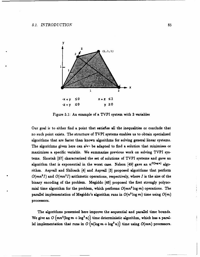
5.1. INTRODUCTION 85
y
-x+y <0 x+z :2
-z+y <0 y >O
Figure 5.1: An example of a TVPI system with 3 variables
Our goal iE to either find a point that satisfies all the inequalities or conclude that
no such point exists. The structure of TVPI systems enables us to obtain specialized
algorithms that are faster than known algorithms for solving general linear systems.
The algorithms given here can akn be adapted to find a solution that minimizes or
maximizes a specific variable. We summarize previous work on solving TVPI sys-
tems. Shostak [57] characterized the set of solutions of TVPI systems and gave an
algorithm that is exponential in the worst case. Nelson [49] gave an no(log' ) algo-
rithm. Aspvall and Shiloach [4] and Aspvall [3] proposed algorithms that perform
0(mn3 I) and 0(mn' I) arithmetic operations, respectively, where I is the size of the
binary encoding of the problem. Megiddo [46] proposed the first strongly polyno-
mial time algorithm for the problem, which performs 0(mn 3log m) operations. The
parallel implementation of Megiddo's algorithm runs in 0(n log m) time using 0(m)processors.
The algorithms presented here improve the sequential and parallel time bounds.
We give an 0 (mnl(log m + log' n)) time deterministic algorithm, which has a paral-
lel implementation that runs in 0 (n(log m + log' n)) time using 0(mn) processors.
86 CHAPTER 5. SYSTEMS WITH TWO VARIABLES PER INEQUALITY
An additional improvement is obtained through using randomization: we give an algo-
rithm that runs in 0 (n' log n -! mn(logs n -r log m log3 n)) expected time. A parallel
implementation runs in 0 (n(log' n - log3 n log m)) expected time using O(n 2- M)
processors. The effort involved in translating these algorithms into actual programs
is about the same as in the previously known algorithms, and the hidden constants
in the time bounds are still reasonable. The space requirement of these algorithms
is O(n 2 + M). Hochbaum and Naor [32] found a new O(mn 2 log m) deterministic
algorithm for the problem. Their algorithm, however, runs in O(n2 log M) time in
parallel, and it does not seem possible to combine it with the randomized approach
to yield algorithms with better expected time.
Section 5.2 gives the preliminaries. In particular we discuss the subproblem of
locating a value: for a numerical value and 1 < i _< n, decide whether a TVPI
system with the addition of either zi > or zi < remains feasible. An 0(mn)
algorithm (O(n) time 0(m) processors in parallel) for locating a value was given by
Aspvall and Shiloach [4].
In Section 5.3 we introduce a framework for solving TVPI systems and analyze
the running time of a deterministic algorithm that relies on locating values. We use
this framework to reduce solving TVPI systems to solving a polylogarithmic number
of instances of the more general subproblem of locating a pool of values: for numerical
values 4,... ,4, choose bounds s1,... , s,,, where si E {i > fi, zi < fi}, such that the
system with the additional constraints s a,..., s. remains feasible. Obviously, a pool
of values can be located by n sequential applications of an algorithm that locates a
single value. This yields an 0(mn2 ) time sequential algorithm which in parallel, runs
in 0(n 2 ) time using 0(m) processors.
In Section 5.4 we present better algorithms for locating a pool. We first give an al-
gorithm that improves the parallel running time to 0(n) using 0(mn) processors. We
also give an overview of a two stage ((mn) time randomized algorithm. Sections 5.5
and 5.6 are concerned with the details of the two stages.
In Section 5.7 we discuss the special structure of monotone systems. Section 5.8
contains concluding remarks.
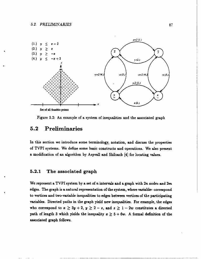
5.2. PRELIMINARIES 87
X+2 (.)
(1.) y < z--2
(2 .) y > T
(3.) y > ->(4.) y < - 22
Y
-v+~2 (4.) -X (3.) -x+2 (4.) -v(3.)v+-2 U.)
. . . . . . . .. . ."| ". " .'"
,*s.. )..** . %€:
X X
Set of all feasible points
Figure 5.2: An example of a system of inequalities and the associated graph
5.2 Preliminaries
In this section we introduce some terminology, notation, and discuss the properties
of TVPI systems. We define some basic constructs and operations. We also present
a modification of an algorithm by Aspvall and Shiloach [4] for locating values.
5.2.1 The associated graph
We represent a TVPI system by a set of n intervals and a graph with 2n nodes and 2m
edges. The graph is a natural representation of the system, where variables correspond
to vertices and two-variable inequalities to edges between vertices of the participating
variables. Directed paths in the graph yield new inequalities. For example, the edges
who correspond to x > 3y + 2, y _> 2 - z, and z > 1 - 2w constitutes a directed
path of length 3 which yields the inequality z > 5 + 6w. A formal definition of the
associated graph follows.
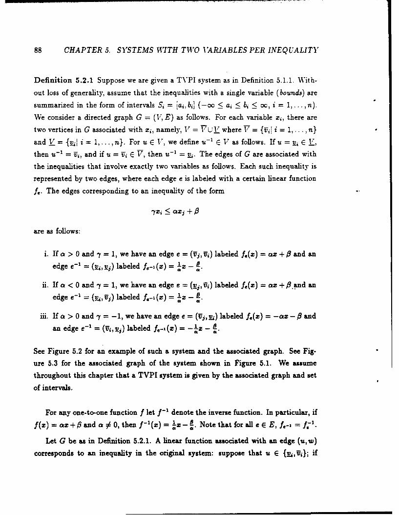
88 CHAPTER 5. SYSTEMS WITH TWO VARIABLES PER INEQUALITY
Definition 5.2.1 Suppose we are given a TVPI system as in Definition 5.1.1. With-
out loss of generality, assume that the inequalities with a single variable (bounds) are
summarized in the form of intervals Si = [ai, bil (-oo < ai < bi < oc, i = 1,... In).
We consider a directed graph G = (V) E) as follows. For each variable xi, there are
two vertices in G associated with xi, namely, V = Vu_ where V = { i! i = 1,... ,n}
and V= {J i= 1,...,n}. Foru E V, wedefineu - 1 E V asfollows. Ifu =i_1 EL,then u - ' = i, and if u = Ui E V, then u - 1 = vi. The edges of G are associated with
the inequalities that involve exactly two variables as follows. Each such inequality is
represented by two edges, where each edge e is labeled with a certain linear function
fe. The edges corresponding to an inequality of the form
7zi < CaZ. + 8
are as follows:
i. If a > 0 and7= 1, we have an edge e = (V, j) labeled f.(z) = az + and an
edge e- - (,, i) labeled f.-i(z) = -
ii. If a < 0 andy= 1, we have an edge e =(, ) labeled f.(z) = az + j6and an
edge e 1 = (v,,Ij) labeled f.-i(z) = -
iii. If a > 0 and y = -1, we have an edge e = (j,v) labeled f.(z) = -am - and
an edge e- ' = (Ui, ) labeled f-i(r) = -- x - !.
See Figure 5.2 for an example of such a system and the associated graph. See Fig-
ure 5.3 for the associated graph of the system shown in Figure 5.1. We assume
throughout this chapter that a TVPI system is given by the associated graph and set
of intervals.
For any one-to-one function f let f- denote the inverse function. In particular, if
f(m) = a + 67 and a # 0, then f-'(z) = - !. Note that for all e E E, fe-i = f-.
Let G be as in Definition 5.2.1. A linear function associated with an edge (u, w)
corresponds to an inequality in the original system: suppose that u E {f, iv}; if
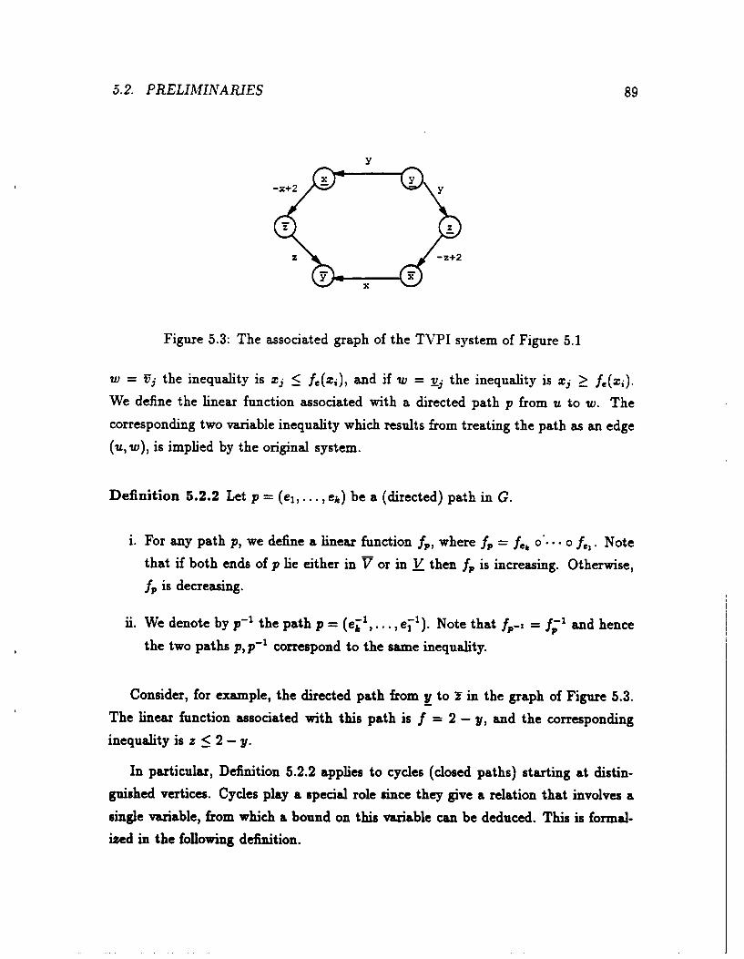
5.2. PRELIMINARIES 89
-x+ Y z
Figure 5.3: The associated graph of the TVPI system of Figure 5.1
w = VY the inequality is xj <: fe(zj), and if w = j__ the inequality is zj >_ fe(xi).
We define the linear function associated with a directed path p from u to w. Thecorresponding two variable inequality which results from treating the path as an edge
(u, w), is implied by the original system.
Definition 5.2.2 Let p = (el,. ., ek) be a (directed) path in G.
i. For any path p, we define a linear function fp, where fp = f, o'... o f,. Notethat if both ends of p lie either in V or in V then fp is increasing. Otherwise,
fp is decreasing.
ii. We denote by p-1 the path p = (ek,..., e,'). Note that fp-i = f;' and hence
the two paths p, p-1 correspond to the same inequality.
Consider, for example, the directed path from y to I in the graph of Figure 5.3.The linear function associated with this path is f = 2 - y, and the corresponding
inequality is z < 2 - y.
In particular, Definition 5.2.2 applies to cycles (closed paths) starting at distin-guished vertices. Cycles play a special role since they give a relation that involves a
single variable, from which a bound on this variable can be deduced. This is formal-
ized in the following definition.
90 CHAPTER 5. SYSTEMS WITH TWO IARIABLES PER INEQUALITY
Definition 5.2.3 We extend the definition of a cycle to paths starting at v and
ending either at v or at v-1 .
i. Let c be a cycle starting at one of the vertices Vi and L, and ending at a
vertex Vi (resp., vi). Let fc be the associated linear function. The bound on zi
implied by the cycle c follows from the inequality x < fc(z) (resp., x > f.(z)).
Obviously, the implied inequality must hold for all feasible points. Note that if
a cycle c starts at Fi and ends at v (resp., starts at v and ends at Vi), then fc
is decreasing. Hence, c implies a lower bound (resp., an upper bound) on Xi.
ii. We say that the cycle c contradicts a value i of Yi (resp., x) if the bound
implied by c is of the form zi _> a (resp., xi _< a) whereas i < a (resp., i > a).
Consider the graph of Figure 5.2 and the cycle which consists of the path from x
to X. The function associated with this cycle is f = -z + 2 and the bound implied
by the cycle is z < -z + 2 (i.e., x < 1).
5.2.2 Pushing bounds along edges
We maintain numerical values associated with the vertices of G; the value associated
with Vi (resp., v) is denoted by Yj (resp., x.). Intuitively, Yi and x- correspond to
upper and lower bounds, respectively, on the value of the variable xi. We say that
is tighter than A as a value of Y, (resp., &-), if < p (resp., C > ji). We introduce the
following operation which considers an edge (u, v) and updates the bound associated
with v, as implied by the inequality associated with (u, v) and the bound associated
with u.
Definition 5.2.4 A push through an edge e is defined as the following operation:
i. If e = (Uj,U), m, -min{i,, f,(Yj)}.
ii. If e = (v-, v), x maxf ~,/(z )I.
5.2. PRELIMINARIES 91
iii. If 6 = (Vj,"t), 'X - max{j x , }
iv. If e = (j_ ,;U), Y, min{5,, f,(I_)}.
A push is said to be essential if it actually modifies the value of - or xi.
Proposition 5.2.5 Suppose x and Y. (i = 1,..,n) are initialized to any values and
let X be the set of vectors z = (Xi,. .7. ,,)T which (i) satisfy all the given inequalities
and (ii) T < xi <. (i = 1,... ,n). The set X is invariant under pushes.
Proof: Consider any z E X and a push through an edge e = (ii,i). (The
arguments for the other cases are similar.) Since z is a feasible solution we have
xi _ fe(xj). Note that f. is an increasing function when both ends of e lie either
in V or in V. Hence, from xj _< Yj, it follows that zi <_ f.(Yi). Since xi < fi, we
have zi _< min{f.,fe(zj)}. I
It is easy to see that a vector z solves a given TVPI system if and only if (i)
zi E Si (i = 1,... ,n) and (ii) the set of values j = zi (i = 1,... ,n) is invariant
under pushes.
We define a new operation which amounts to pushing (see Definition 5.2.4) through
all the edges simultaneously. This operation is used as a subroutine in algorithms
presented later in this section.
Definition 5.2.6 Consider the graph G with some set of values at the vertices, x =
4 i (i - 1,..., n). A push phase on G is assigning, at the respective vertices,
the set of values -+i, - + ' (i = 1,...,n) defined as follows:
Yi*+ min ei 1', } i f.(?-) if e =(Vj,;), or .()if e=
mmo + -- ran{ a {f.(I) if e = (v.,j), or .(_) ife=
Consider repeated applications of push phases. The initial set of values is denoted
by j, , = ii (i = n,...,L), and z and fi denote the respective values of .
92 CHAPTER 5. SYSTEMS WITH TWO VARIABLES PER INEQUALITY
and Yj after the termination of the k'th push phase.Consider pairs consisting of a value and a vertex, (_4, ) and (', i:)(where k > 0
and 1 < j < n). The predecessor of a pair ( , v) is the pair (', v') such that e = (v', v)
is the edge through which the essential push determined the value , and C' =f-1(6)
is the corresponding value at v'. If the predecessor is not uniquely defined we choose
arbitrarily among the qualified pairs. A pair ( , v) does not have a predecessor if and
only if 6 is the initial value at v.
The essential path associated with a pair ( ,v) consists of the sequence of pairs
(G)'VO),..., (41, vj) and the corresponding sequence of edges ej,..., e- 11 such that
(i) ( ,, vi)is the predecessor of ( j+i, vi+i) and ej is the edge through which the essen-
tial push occurs (i = 1,... ,I- 1), (ii) (Cl,vj) = (C,v), and (iii) (Cl,vi) does not have
a predecessor.
It is easy to see that the essential paths which correspond to (, ) and (', VY)
(i = 1,..., n) can be found within the same time bounds of performing I push phases,
simply by keeping track of all essential push operations.
We extend the notion of a push through an edge to directed paths. Let p =
(ei,... , ek) be a (directed) path in G. A push along p is defined to be the composition
of k successive pushes, through the edges ej,..., ek.
5.2.3 Properties of the feasible region
Consider the bounds on the variables which are implied by directed cycles. We
discuss the relation of these bounds to the feasible region. We first give the following
definitions.
Definition 5.2.7 i. For each variable xi, let (x:, I] C (a, bi] be the set of values
which are not contradicted by any simple cycle. Note that the two cycles c and
c-1 imply the same bound. It follows that in order to find Y (resp., C.), it
suffices to consider cycles ending at Ui (resp., v).
5.2. PRELIMINARIES 93
ii. Denote by , , inaxC [ x- -'" the largest interval such that (1) for all simple
paths p from a vertex Tj (resp., Lj) to Ti we have mxT" < fp(Y;) (resp., x' x <
fp(g_;) ) and, (2) for all simple paths p from a vertex Uj (resp., Kj) to v.. we haveXi n > (y;) (resp., xi n > fPz.).
iii. An interval I C R is infeasible with respect to the variable xi if I [xinX , nax] =
0. A value Yj (resp., x) is infeasible if 1i < x (resp., g_ > m1").
iv. A value Yi (resp., zi) is consistent with an interval [a, b] if Y, > b (resp., & < a).
Remark 5.2.8 When the values T and g_, (i = 1,..., n) are given, we can computemin a~Xi and z ax as follows. Initialize the values at the vertices to be z, = Y and09= z (i = 1,... In). Perform 2n push phases. It follows from Definition 5.2.7
part ii that x = ki and 2T'a = Y. This procedure runs in O(mn) time and is
used in Megiddo's algorithm [46].
For example, the TVPI system of Figure 5.2 has lk, Y] = 1-1, 1] = [,n, xm"], and
[Y,V] = [0, 7] = rain ,y']. The TVPI system of Figure 5.3 has [Z',Y] = [1_,!] =
[-0o,+oo], [y-, V] = [y-, yma] = [0,1], and ['r , .1] = [z ,z-] = [0,2].
The following key observation is due to Shostak:
Proposition 5.2.9 [57] If the system is feasible, then -the interval [zr, zP ] is the
projection of the set of solutions on the zi-azis. Otherwise, zm > z =a for some
<i<n.
The proof follows from considering the possible structure of minimal sets of in-
equalities which imply a bound on a variable. Proposition 5.2.9 and the procedure
described in Remark 5.2.8 assert that it suffices to consider all simple paths and cy-
cles in the associated graph. Shostak presented an exponential time algorithm that
essentially examines all directed simple cycles [57].
The following corollary states that if two bounds are feasible separately but not
simultaneously, then there exist a simple path that implies an inequality which asserts
that the bounds are not simultaneously feasible.
94 CHAPTER 5. SYSTEMS WITH TWO IARIABLES PER INEQUALITY
Corollary 5.2.10 Let S be a set of TIPI constraints, and s, E {xi _> a., i a}
s2 E {xj >1 aj K 3} be two bounds. Let ui = Fi if s, is an upper bound, and ui = v
otherwise; and let uj = Uj if 52 is an upper bound, and uj = Ij otherwise. Suppose
S U {sI}, and S U {s 2} are feasible systems, but S U {sI, S2 } is not feasible. There
exist a simple path p from ui to uI such that (i) fp(a) < 8, if s 2 is a lower bound,
and (ii) fp(ca) > 1, if s2 is an upper bound. Moreover, if p is the tightest (simple)
path from ui to uj-1 relative to x = a, then if S2 is an upper (resp., lower) bound,
xj = fp(a) is the smallest (resp., largest) value of x3 subject to S U {sI}.
Proof: Suppose that both 81,S2 are upper bounds (similar for the ot~ier cases).
Consider bj = z 5 under the system S U {so } and b, = x, under the system S.
We have b < 8 and b3 > 1. By definition, xz" is either (a) implied by a cycle
or a cycle and a path (i.e., implied only by inequalities which involve exactly two
variables), or (b) implied by a single variable inequality involving some variable
xj and a (possibly empty) directed simple path. Since the system S contains the
same two variable inequalities as S U {si}, bj is determined by a system of type (b)
consisting of the bound al and a simple path p. *
5.2.4 Characterizations of TVPI polyhedra
Proposition 5.2.9 characterizes the feasible region in terms of the associated graph.
We characterize polyhedra which comprise sets of solutions of TVPI systems (TVPI
polyhedra). Polyhedra which can not be expressed as such are non-TVPI polyhedra.
Proposition 5.2.11 Consider a polyhedron P C R". The following statements are
equivalent:
i. The polyhedron P is a TVPI polyhedron.
ii. For a bounded convez set P' = PflB', where B' is a box, denote ai = minzTp, :i,
bi = max P'zi (i = 1,...,n), and denote by B = X!f[ai,4,b] the tightest
bounding bo: for P'. Every P' as above is such that la + 1b E P'.
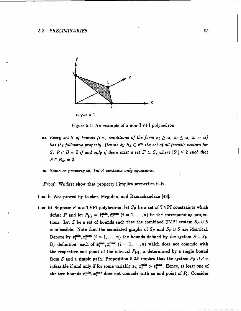
5.2. PRELIMINARIES 95
Y
1 z
x+y+z = 1
Figure 5.4: An example of a non-TVPI polyhedron
iii. Every set S of bounds (i.e., conditions of the form xi > a, z i a, za = a)
has the following property. Denote by Bs E R" the set of all feasible vectors for
S. P B =0 if and only if there exist a set S' C S, where IS'I < 2 such that
PfnBs, = 0.
iv. Same as property iii, but S contains only equations.
Proof: We first show that property i implies properties ii-iv.
i => ii Was proved by Lueker, Megiddo, and Ramachandran [43].
i => iii Suppose P is a TVPI polyhedron, let Sp be a set of TVPI constraints which
define P and let Pi} = iie' (i = 1,..., n) be the corresponding projec-
tions. Let S be a set of bounds such that the combined TVPI system Sp U S
is infeasible. Note that the associated graphs of Sp and Sp U S are identical.Denote by z , :" x (i = 1,..., n) the bounds defined by the system S U Sp.B' definition, each of : , z~" (i = 1,... ,n) which does not coincide with
the respective end point of the interval P~i), is determined by a single bound
from S and a simple path. Proposition 5.2.9 implies that the system Sp U S is
infeasible if and only if for some variable z, zz > zxf. Hence, at least one of
the two bounds zi , " does not coincide with an end point of P. Consider
96 CHAPTER 5. SYSTEMS WITH TWO I ARIABLES PER INEQUALITY
the bounds S' C Sp -. S (;S'. < 2) which determine xin > XT ax. Obviously.
the system Sp j S' is infeasible.
in > iv Obvious.
It remains to prove that ii-iv => i. Note that properties i-iv are invariant under
scalings and translations of coordinates.
Figure 5.4 gives an example of a non-TVPI polyhedron. It is easy to see that for
this polyhedron property ii does not hold (consider the bounding box 0 < z < 1,
0 < y < 1, 0 < z < 1), and property iv does not hold (consider S = {x = 0,y V
0,z = 0}).
Assume that P is a non-TVPI polyhedron. There exist at least one face F such
that the following holds. Let A E R x'" , b E R' be such that {z E Rn I Am = b} is
the affine hull of F. Consider the process of eliminating variables from the system
Am = b, until no two equations involve the same variable. At least one of these
equations involves more than two variables. Consider such a face F. Without loss of
generality (by scaling coordinates) we can assume that the equation is E mi = 1
(where I > 3), and for all points z E P, z :, 1. Denote by H the hyperplane
H = {zI Ef=1 Zi = 1}. It is easy to see that the construction is such that the
projection P' C H of P on H is full-dimensional, that is, affP' = H. Consider a
point i E relint P'.
iv =; i By definition, there exist a small enough c > 0 such that for i = 1,..., 1,
there exist m' E P such that z' = i - (I - 1)c, and x' = ii + e U
1,i +..., ). Consider the set of equations S = {zj = ii + el j - 1,...,t}.
Obviously, there is no point in P which satisfies S. On the other hand, there is
a point which satisfies every subset of I - 1 > 2 constraints. Hence, property iv
does not hold for P.
ii = i By definition, there exist a small enough e > 0 such that for i = 1,..., 1,
there exist m E P such that z = ii + (I - 1)e, and zi = j - e U
1, i + 1, 1). Consider the box B defined by the intervals [j - e, il + ( - 1)e
5.2. PRELIMINARIES 97
(i = 1,...,1). Since x i E B n P, B is a bounding box for B P. However,
there is noz E P for which xj = j (I - 2)f (j = 1,...,). It follows that
property ii does not hold for P.
5.2.5 Locating values
We discuss two procedures which are used later in the paper and are based on repet-
itive applications of push phases and examining essential paths.
One of the procedures solves the following problem.
Problem 5.2.12 [Locate a value] For a given TVPI system, a number and a vari-
able zi, locate with respect to the interval [zx" , zf], that is, decide whether (i)j< Xmn > z ,or E(zin "
We refer to solving Problem 5.2.12 as locating the value i. Aspvall and Shiloach [3,
4] proved the following:
Proposition 5.2.13 Problem 5.2.12 can be solved in O(mn) operations.
Aspvall and Shiloach utilized this result to solve TVPI systems: by solving in-
stances of Problem 5.2.12 their algorithm conducts a binary search which finds a
point i E [zfni', : ] (1 < i < n). They showed that finding such a point fi can be
done in O(mnI) operations where I is the number of bits in the binary representation
of the input. This yielded their O(mn2 I) algorithm for TVPI systems: the algorithm
performs n steps, where in step i a point fi E [zi, z'-] is found, and the equation
zi = fi is added to the system. If the original system is feasible, then 4 E F.
In Section 5.3 we present a O(mn2) determiistic algorithm for solving TVPI
systems, which is based on locating values in the time bounds stated in Proposi-
tion 5.2.13. The material contained in the remainder of the current section is needed
98 CHAPTER 5. SYSTEMS WITH TWO IARIABLES PER INEQUALITY
for achieving the randomized bound of 6(n 3 - rnn) and improving the parallel com-
plexity of solving TVPI systems. We present and analyze an algorithm for locating
values which is also applicable to the reveal problem which is defined later. The
underlying computation amounts to 0(n) applications of push phases where essential
paths are maintained.
Certificates of infeasibility: Suppose an interval I = [a, b] is infeasible with re-
spect to zi (equivalently, either [-oc, b] or [a, 00] is infeasible). It follows from Propo-
sition 5.2.9 that there exist a vertex w, a simple path p from u E {v.,, Vi} to w, and
a disjoint simple cycle starting at w such that the bound on w implied by c and the
path p produce a bound on zi which does not intersect I. The path p and the cycle
c form a minimal subsystem which implies the infeasibility of I. Note that the cycle
c may be empty in which case the infeasibility follows from the path p and a bound
on the variable associated with w. We refer to such a system as a certificate for I.
If c starts and ends at u, we say that the certificate is closed. If c ends at u- ' or
c is empty, we say that the certificate is open. When we refer to a certificate, we
interchangeably mean the set of edges E' = p U c, the set E'- ' of the reversed edges,
or the corresponding set of inequalities.
Classifying values: We classify values of variables according to the types of their
certificates. Consider an interval I with respect to zi. If I has a closed certificate we
say that I is strongly infeasible. If only open certificates exist, we say that I is weakly
infeasible. Otherwise, if no certificate exists, I n [m:in, z'P] 0 and we say that I is
feasible.
In particular this definitions apply when I consists of a single point. For 1 < i < n,
we denote by [znI' , zP'] the set of all feasible and weakly infeasible values of mi.
Note that x i , (1 < i < n) are independent of the single variable inequalities.
We extend the definitions of the concepts above from intervals to values at vertices
of G: A property (having a closed/open certificate, weak/strong infeasibility) holds
for a value f at a vertex vi (resp., Vi) if it holds for the interval [C, oo] (resp., [-00, ])
with respect to mi.
5.2. PRELIMINARIES 99
We present two corollaries of Propositions 5.2.5 and 5.2.9. Consider a feasible
TVPI system and the associated graph. Suppose a sequence of push phases is per-
formed.
Corollary 5.2.14 If the values at the vertices are initially consistent (see Defini-
tion 5.2.7), they remain consistent after any number of push operations.
Corollary 5.2.15 Consider a vertex u = v (resp., u, = v,) and a value = f (resp.,
= Y'1) for some £. Let ( ,,vj) (j = 1,... ,k < 1), where (4,vk) (= ,), be the
pairs comprising the essential path (see Definition 5.2.6) associated with ( , u). If
is infeasible (resp., strongly infeasible) at u, then each of the pairs (c,, v3 ) (1 < j < k)
is such that j is an infeasible (resp., strongly infeasible) value of vj.
Consider an essential path which contains a cycle (a vertex appears more than
once). The following proposition enables us to extract information from the cycle. It
states that either all values following the start pair of the cycle are consistent (the
path does not add information) or all values preceding the last pair of the cycle are
strongly infeasible (an infeasible value is detected). Moreover, by considering the
updating cycle we can determine which of the two situations occurs.
Proposition 5.2.16 Let be a value at u = Ui (resp., u = ,). Suppose a cycle c,
which starts and ends at ,) is such that ff) < f (resp., f,( ) > f). Then, either
(i) C is strongly infeasible at u and the cycle c is a closed certificate, or (ii) if F # 0,
is consistent at u.
Proof: The bound implied by the cycle c is fe(y) _! y (resp., .f(y) < y). It suffices
to show that it holds either (i) only for values y such that y _> e, or (ii) only for
values y such that y < f. The function f,(y) - y is linear and thus can change sign
only once. It cannot be a positive (resp., negative ) constant, since this contradicts
f,(C) being tighter than f. If the function is a negative (resp., positive) constant,
the cycle implies that the system is infeasible (and therefore f is contradicted by
100 CHAPTER 5. SYSTEMS WITH TWO IARIABLES PER INEQUALITY
the cycle). Otherwise, consider the value y- such that f,(y-) = y'. It is immediate
that the bound implied by c and the number 4 are on opposite sides of y-. I
The following algorithm is applied to a set of values x, 'xi (for 1 < i < n). The al-
gorithm performs a sequence of push phases, and keeps track of essential paths. When
the algorithm detects a non simple essential path, it either terminates or discards the
path. If the algorithm terminates as a result of such a path, a closed certificate is
found for one of the initial values. A vertex v is active at a particular point in the
execution of the algorithm if the current value at v resulted from an essential path
which is not discarded.
Algorithm 5.2.17
i. For i = 1,... ,n, initialize the values at v. and i as zo and 2-j, respectively.
ii. For k = 1,..., 2n do steps iii-vii. If the algorithm did not terminate, determine
that none of the initial values is strongly infeasible, and stop.
iii. Perform a push phase. Denote the values at the vertices after the k'th push
phase by z, 4 (1 < k < 2n).
Keep track of all essential push operations which result from active vertices. If
there are no such essential pushes or no active vertices, stop and determine that
none of the initial values is strongly infeasible.
(We assume that ambiguities about the edge which carried the essential push
are resolved consistently according to some ordering on the edges.)
iv. If k # 2j for all integers j and k $ 2n, go to step iii (next iteration).
v. Optional: If for some j, z_4 > z-, then stop.
vi. For each active vertex v, let p, be the essential path that corresponds to the
last update of the value at v.
If p, contains a cycle (i.e., some vertex appears in more than one pair), execute
step vii. After considering all vertices, go to step iii (next iteration).
5.2. PRELIMINARIES 101
vii. Consider the last simple cycle c on p,. Denote by u the vertex where the
cycle starts and ends. Denote by the value associated with u at its first
occurrence on the cycle. Check whether the bound implied by c contradicts t.
If there is no contradiction, t is consistent (see Proposition 5.2.16), discard all
essential paths originating from the first pair (u, t) of the cycle (all correspond
to consistent values according to Corollary 5.2.14); proceed to consider the
next vertex. Otherwise, if c contradicts t, 4 is strongly infeasible. It follows
from Corollary 5.2.15 that so are all values along the path p, prior to the pair
(u, f,(t)) (the last occurrence of u on p,,). In particulr, the initial value at the
first vertex w of p, is strongly infeasible. Stop.
Complexity: The underlying computation of the algorithm is the Bellman-Ford
single-source shortest path computation [13], where we maintain information needed
to construct the paths and test for cycles.
The algorithm terminates after I < 2n iterations, in which case, it requires 0(ml)
sequential time, and 0(1) time using 0(m) processors on a CRCW PRAM.
If the algorithm terminates at step vii, it finds a closed certificate for the initial
value at w. If the algorithm terminates during the t'th iteration, the closed certificate
found is of size 8(1).
Proposition 5.2.18 Consider an ezecution of Algorithm 5.2.17, where step v is
skipped.
i. At least one of the initial values is strongly infeasible if and only if the algorithm
terminates at step vii.
ii. Suppose ezactly one of the initial values, t at the vertex w, is strongly infeasible.
The algorithm terminates at step vii with the same closed certificate regardless of
the initial values at other vertices. We refer to this certificate as the certificate
Of 4.
Proof: We first prove part i. The "if" direction is immediate. Suppose an initial
value f at a vertex w has a closed certificate consisting of a path p of length IjP to uo
102 CHAPTER 5. SYSTEMS WITH TWO VARIABLES PER INEQUALITY
and a cycle c of length r which starts and ends at uo. After at most ,p. iterations,
the value at u0 is at least as tight as fp( ) and hence, has a closed certificate
consisting of c. Similarly, after jp[ + r iterations the same holds for all the vertices
of c. Let eo, ... , e, and uo,. . . , u., respectively, be the edges and vertices of c. We
claim that all iterations for which k > I result in an update of at least one of
the values at uo,... u,.. Assume the claim is true. Suppose the algorithm did not
terminate during any of the 2n iterations. It follows that at least one of the paths
p,j (1 < j _< r) is of length 2n, and hence, contains a cycle. Since the value at uj
is strongly infeasible, it follows from Corollary 5.2.15 that w is the first vertex of
PUj. It follows from Proposition 5.2.16 that each cycle in p,, contradicts the value
at the start vertex.
What remains is to prove the claim. Assume the contrary. Let 0,...,, be the
respective values at uo,... , u,. In particular, none of the edges ek had an essential
push. Hence, for all j = ... ,r, f,(4j) is not tighter than j+1mod,. It follows
that fei..,,( o) = f.(4o) is less tight than o. This is a contradiction for c being a
closed certificate for fo.
We prove part ii. Consider an initialization where at wv is the only strongly
infeasible value. It follows from part i that the algorithm terminates in step vii,
and finds an essential path p which starts at w and terminates in a cycle. All values
along the path are strongly infeasible. Suppose that an initial path starting at a
vertex other than tw updates a value at a vertex in p. It follows from Corollary 5.2.15
that the updated value can not be tighter or as tight as the value resulting from p.
The proof follows. I
Remark 5.2.19 Consider a run of the algorithm where step v is performed.
i. Suppose that the algorithm terminates at step v, where it detects -- > z-*.
Consider the initial pairs (u, C) and (w, p) of the two essential paths which
determined (v,_4) and (,uj,y!). It is not necessarily true that one of the ini-
tial pairs is infeasible. We can conclude, however, that the two corresponding
bounds can not be satisfied simultaneously by a feasible vector.
5.2. PRELIMINARIES 103
ii. Consider a run of the algorithm where at least one of the initial values has
an open certificate of size £ which contains a nontrivial cycle. The following
is immediate: the algorithm terminates at either step vii or step v within I
iterations.
Locating a value: We apply Algorithm 5.2.17 to solve Problem 5.2.12.
Consider a value j. We show how to decide whether or not i > Tax (the case
i < Xm is similar).
Algorithm 5.2.20 [Locate a value with respect to 2 max]
Perform a run of Algorithm 5.2.17, where step v is enabled, for the following input
of values:
x9 = aj for j 0 i, 2 = bj for j = 1,..., n, and 9 = ,.
Conclude as follows:
" If the algorithm stopped at step iii (no active vertices), determine that j :5 z 1 .
" If the algorithms stopped at step v, consider the essential paths associated with
k > 2. If in neither path, the initial pair is (v, t), conclude that the system
is infeasible. Otherwise, conclude that t, > xa.
" Suppose the algorithm terminated at step vii. If w = ,, determine that . >
z" . Otherwise, if -4 , the system is infeasible.
" If the algorithm terminated at step ii, determine that t, < x .
The correctness follows immediately from Proposition 5.2.18 part i, and Re-
mark 5.2.19.
Reveal a strongly infeasible value: We discuss applying Algorithm 5.2.17 to
solve the following problem.
104 CHAPTER 5. SYSTEMS WITH TWO 1ARIABLES PER INEQUALITY
Problem 5.2.21 Reveal a strongly infeasible value]
Given are values j, ai :_ i <_ bi (i E 1) for the respective variables zi (i - I), where
I C{1,...,n}. Do one of the following:
i. Conclude that all the values are feasible or weakly infeasible.
ii. Find a strongly infeasible value j and a closed certificate.
Algorithm 5.2.22 [Reveal]
Perform a run of Algorithm 5.2.17, where step v is skipped, for the input values:
Yi = x = (i E I), and Yi = hi, x = ai (i I).
The following is a corollary of Proposition 5.2.18:
Corollary 5.2.23 Algorithm 5.2.22 solves Problem 5.2.21. If none of the initial
values is strongly infeasible, the algorithm requires O(mn) operations. Otherwise, the
algorithm terminates after I < 2n iterations with a closed certificate of size 0(l). If
ezactly one of the values 4i (i E I) is strongly infeasible, the algorithm terminates
with the same closed certificate regardless of the other values.
5.3 The basic algorithm
In this section we present a framework for solving TVPI systems. This framework
allows us to state an algorithm for TVPI systems in terms of solving instances of
Problem 5.2.12 (locating single values). The framework is stated in Subsection 5.3.1,
and the correctness proof is given in Subsection 5.3.2. In Subsection 5.3.3 we reduce
solving a TVPI system to locating O(n(log2 n +log m)) values. Since locating a single
value requires O(mn) time (O(n) time in parallel) (see Proposition 5.2.13), we obtain
an O(mn2(log2 n + log m)) deterministic algorithm for solving TVPI systems, which
runs in 6(n') time in parallel.
In Subsection 5.3.4 we introduce the problem of locating a pool of values. A key for
further improvements is reducing the solution of a TVPI system to locating O(log2 n-i-
5.3. THE BASIC ALGORITHM 105
log m) pools of values. A pool of values can be located naively by sequentially locating
n single values. In Section 5.4 we present faster parallel and sequential algorithms forlocating a pool, which yield better algorithms for solving TVPI systems.
5.3.1 The framework
We first describe an idea introduced by Megiddo [46], which is the key in obtain-
ing strongly polynomial time bounds. Consider the associated graph of some TVPI
system. Every directed path in the associated graph corresponds to a two-variable in-equality. Consider two inequalities which correspond to two paths between the same
pair of vertices (vi, vj), where vi E { i, L}. These inequalities are linear, hence, there
exists a number a such that for all xi _< a one of the inequalities implies the other,
and vice versa for xi _> a. If we focus only on feasible points x for which xi >_ a
(similarly zi _< a), one of the inequalities is redundant.The algorithm eliminates paths and simultaneously restricts the feasible region. When"comparing" two paths, the decision about which one to eliminate is done as follows.
First, the number a, as above, is computed. The redundant path is determined by
locating a with respect to feasible values of xi (see Problem 5.2.12).
Megiddo applied the above idea in an algorithm which basically performed n single-source shortest path Bellman-Ford type computations, where comparisons amount to
locating values. The framework presented here is based on performing an all-pairs
shortest path Floyd-Warshall [13] type computation which allows us to apply further
ideas.
The following definition formalizes the concept of comparing paths.
Definition 5.3.1
i. Suppose that pi and p2 are two directed paths from u to v, and from v to w,
respectively. Denote by P1P2 the path from u to w obtained by concatenating
p, and p2.
106 CHAPTER 5. SYSTEMS ITH TWO VARIABLES PER INEQUALITY
ii. Suppose that p, and P2 are two paths from u to w. Let I C R be an interval.
We say that the path P, is at least as tight as P2 relative to I (denote it by
P1 -"I P2) if either w E L' and fp,( ) > fp,(C) for all C E I, or w E 7 and
& ,(C) < &(C) for all C I.
iii. Suppose p1,p2, ...,pk are paths from u to w. If for some i, pi -<I pj for all j,
we write pi = min..<{p,p 2 ,... ,Pk}. Note that when I is a single point, min,,
is well-defined.
The algorithm maintains a set of intervals Si (1 < n), and a path p, from u
to w for every pair of vertices (u, w). The algorithm runs in [log2 2n1 phases. During
each phase, the paths and the intervals are considered for possible updates. Denote
by Sj' (1 < i < n) and pk,, ({u, w} _ V) the intervals and paths, respectively, at thebeginning of the k'th phase. The algorithm has the following properties: (i) The set
X~ S' , contains a feasible point, and (ii) the path p, is the tightest path from u tow, of length at most 2k, relative to the interval S (where u E {ih, v_i}).
The algorithm is based on solving instances of the following problem:
Problem 5.3.2 Given are a graph G and a set of intervals Si,..., S' as in Defini-
tion 5.2.1. For every ordered pair (u,,v) E V x V of vertices we are given ph,... ,pt,',
a collection of directed paths from u to v in G. The goal is to find a set of n intervals
I1,... , I. and select a path p:, E {pu, ..., p!" } for every pair (u, v) of vertices, where
i. F # 0 : (X_-I,) n F # 0, and
ii.u E{v-;Ui =>p;.= nin.,qj pu',,...,p) "}.
We later suggest algorithms for Problem 5.3.2. The following algorithm uses it
as a subroutine. It first initializes the tightest-paths matrix by selecting the tightest
edge out of every set of multiple edges (step ii). The rest of the algorithm consists of
Rog 2n1 update phases of the tightest-paths matrix (step iv). During each phase, the
algorithm considers n2 sets of n paths (one for each pair of vertices). It then selects
the tightest path in each set. In the last step, the tightest path matrix is used to
compute a feasible vector.
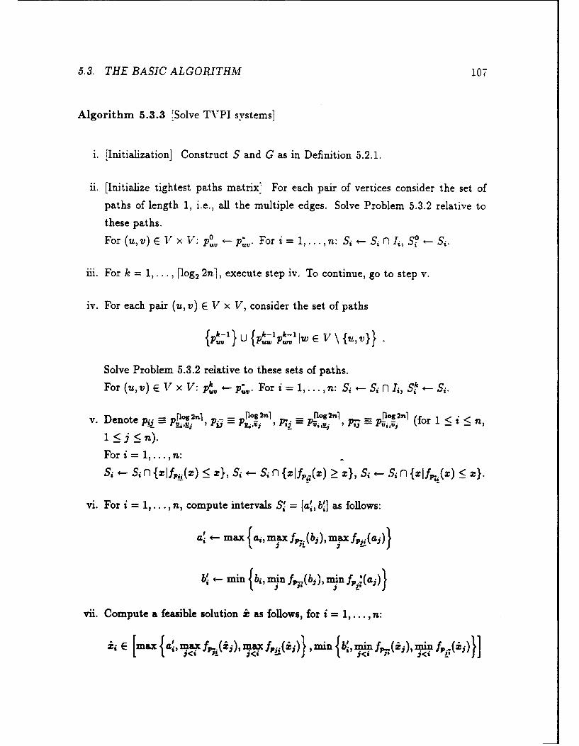
5.3. THE BASIC ALGORITHM 107
Algorithm 5.3.3 fSolve TVPI systems]
i. [Initialization] Construct S and G as in Definition 5.2.1.
ii. [Initialize tightest paths matrix] For each pair of vertices consider the set of
paths of length 1, i.e., all the multiple edges. Solve Problem 5.3.2 relative to
these paths.
For (u,v) E V x V: pO,- p',. Fori=1,...,n: S, *-- Si n ii, sI , - Si.
iii. For k = 1,.. ., [log 2 2n], execute step iv. To continue, go to step v.
iv. For each pair (u, v) E V x V, consider the set of paths
{pU; U {pukw-ipk-1Iw E V u,v}
Solve Problem 5.3.2 relative to these sets of paths.For (,v)E V y xV: p., --p;,. Fori= 1,...,n: s, ,- sini,,s ,i- s,.
v. Denote Py J ' -'.s, __o2,q (for 1 < i < n,_ - ,_ , P6 P-.,j ,I ,,j , / 'l =i i,,<l < ~n).
For i = 1,...,n:
S, <- S, n f lfp,,(.T) <:z}, S, +- S, n f Ijff (.T) > x}, Si +- S n {zlf,,,.(z) <4.V -
vi. For i = 1,... , In, compute intervals Sj' = [ai, bh] as follows:
ai 4-max aimxf,.,(bi)Maxf }
b: 4 mi {b, n~ f (bj), min f, .(aj)
vii. Compute a feasible solution i as follows, for i = 1,... , In:
[max I a' max fp-.(ij), max fvw(i) m in n f, (ij), m~in fpI([max {a~, ,6 '~, - (n
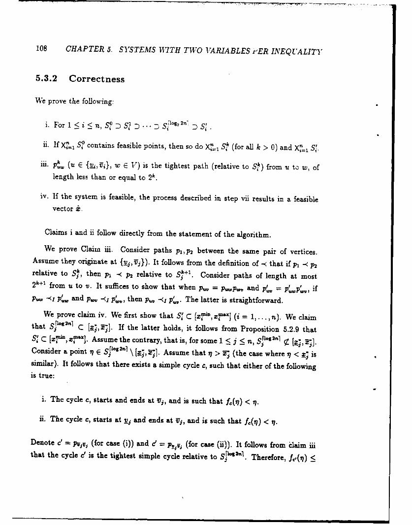
108 CHAPTER 5. SYSTEMS WITH TWO VARIABLES tIER INEQUALITY
5.3.2 Correctness
We prove the following:
i. For 1 < i < n, S°o Si D '"D S11 92 2n ' D S4.
ii. If X!= S° contains feasible points, then so do X 1 Sik (for all k > 0) and X! '.
•i P- , (u E {,,Ui}, w E V) is the tightest path (relative to S ) from u to w, oflength less than or equal to 2k.
iv. If the system is feasible, the process described in step vii results in a feasiblevector i.
Claims i and ii follow directly from the statement of the algorithm.
We prove Claim iii. Consider paths Pi,P2 between the same pair of vertices.Assume they originate at { j, ;j}). It follows from the definition of -< that if pi -< P2relative to 5,", then p, -< P2 relative to S Consider paths of length at most2k+1 from u to v. It suffices to show that when p..' = Pwp. and pt, = pp , ifPW -<I puw and p,. -<I p,, then p,, -<I pu,. The latter is straightforward.
We prove claim iv. We first show that S C [Z , "F] (i = 1,... , n). We claimthat S pog 2 l C [e , j. If the latter holds, it follows from Proposition 5.2.9 thatS C [z" in, zf' ]. Assume the contrary, that is, for some 1 < j n, n,Consider a point 0 E Srog,2nj \ [a;, j]. Assume that 77 " (the case where 7 < k_* issimilar). It follows that there exists a simple cycle c, such that either of the followingis true:
i. The cycle c, starts and ends at U;, and is such that f,(7) < 7.
ii. The cycle c, starts at v, and ends at Uj, and is such that f,(i/) < il.
Denote c' =i, (for case (i)) and c' = p,, (for case (ii)). It follows from claim iiithat the cycle c' is the tightest simple cycle relative to S"" 2 l. Therefore, f (0) <
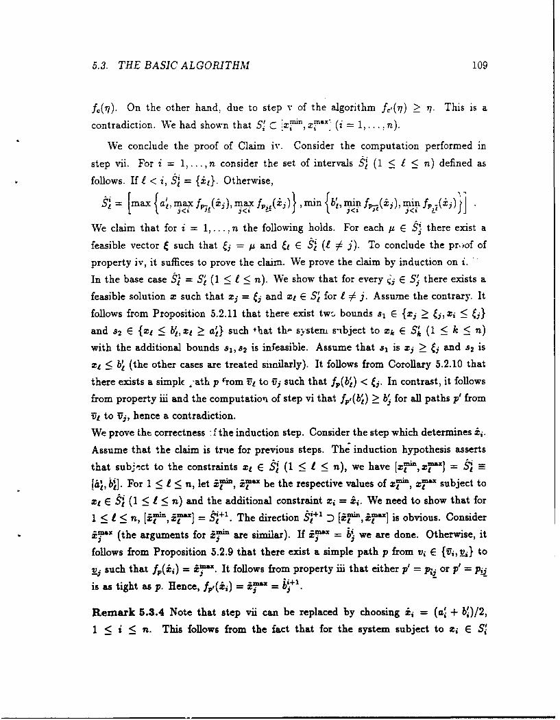
5.3. THE BASIC ALGORITHM 109
f,(in). On the other hand, due to step v of the algorithm f,,(77) > 71. This is a
contradiction. We had shown that S, C , i = 1,... n)
We conclude the proof of Claim iv. Consider the computation performed in
step vii. For i = 1,. . . , n consider the set of intervals Sl (1 < £ < n) defined as
follows. If I < i, i = . Otherwise,
S,= [max a', ma fp- max~ fp,,:c mi m min-(ii ) miiif 3JWe claim that for i = 1...In the following holds. For each IL E Sj' there exist a
^ .7
feasible vector such that j = /t and t E St (I # j). To conclude the pr.,of of
property iv, it suffices to prove the claim. We prove the claim by induction on i.
In the base case S1 = S1 (1 < I < n). We show that for every 'j E S there exists a
feasible solution z such that zj = j and zi E Slt for I j. Assume the contrary. It
follows from Proposition 5.2.11 that there exist tw- bounds si E {j > , zi 5 W
and S2 E {x < b', t 2! a'} such +hat th,' system s-ibject to zk E Sh, (1 < k < n)
with the additional bounds S1, 82 is infeasible. Assume that s, is xj > j and s 2 is
x, < bl (the other cases are treated similarly). It follows from Corollary 5.2.10 that
there exists a simpk -ath p from iTF to 9i such that f,(b,') < i. In contrast, it follows
from property iii and the computation of step vi that fp,(bt) > b for all paths p' from
Ut to vi, hence a contradiction.
We prove the correctness £ the induction step. Consider the step which determines ii.
Assume that the claim is true for previous steps. The induction hypothesis asserts
that subject to the constraints :t E S (1 < I < n), we have [znin, za] = S
[& , b ]. For 1 < 1 < n, let i, i' be the respective values of ' z, subject to
xe S (1 < I < n) and the additional constraint xi = :i. We need to show that for
1 <1 < n, [, i-] = s. The direction Sj+ D [in'n, i"] is obvious. Considerinx (the arguments for i are similar). If F =f . we are done. Otherwise, it
follows from Proposition 5.2.9 that there exist a simple path p from vi E {;Ui, v} to
v, such that fp(ij) = OF. It follows from property iii that either p' = p, or p' = pjj
is as tight as p. Hence, f/,(ii) = i't = b+a
Remark 5.3.4 Note that step vii can be replaced by choosing :i = (a! + b )/2,
1 < i < n. This follows from the fact that for the system subject to zi E Si
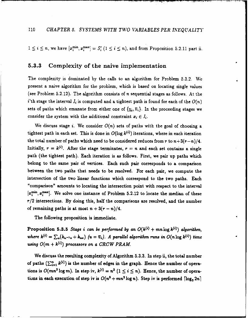
110 CHAPTER 5. SYSTEMS WITH TWO VARIABLES PER INEQUALITY
1 <I < n, we have [xmin, xT1 ] = S (1 < i < n), and from Proposition 5.2.11 part ii.
5.3.3 Complexity of the naive implementation
The complexity is dominated by the calls to an algorithm for Problem 5.3.2. We
present a naive algorithm for the problem, which is based on locating single values(see Problem 5.2.12). The algorithm consists of n sequential stages as follows. At the
i'th stage the interval 1i is computed and a tightest path is found for each of the O(n)
sets of paths which emanate from either one of {v, :U}. In the proceeding stages we
consider the system with the additional constraint zi E Ii.
We discuss stage i. We consider O(n) sets of paths with the goal of choosing atightest path in each set. This is done in O(log k()) iterations, where in each iteration
the total number of paths which need to be considered reduces from r to n+3(r -n)/4.
Initially, r = k(0). After the stage terminates, r = n and each set contains a single
path (the tightest path). Each iteration is as follows. First, we pair up paths whichbelong to the same pair of vertices. Each such pair corresponds to a comparison
between the two paths that needs to be resolved. For each pair, we compute the
intersection of the two linear functions which correspond to the two paths. Each"comparison" amounts to locating the intersection point with respect to the interval
[z", z ]. We solve one instance of Problem 5.2.12 to locate the median of these
r/2 intersections. By doing this, half the comparisons are resolved, and the number
of remaining paths is at most n + 3(r - n)/4.
The following proposition is immediate.
Proposition 5.3.5 Stage i can be performed by an O(k() + mnlog k()) algorithm,
where k() = ,(k,-, + k.,) (u = U). A parallel agorithm runs in O(n log k()) time
using O(m + k()) processors on a CRCW PRAM.
We discuss the resulting complexity of Algorithm 5.3.3. In step ii, the total number
of paths (E' k()) is the number of edges in the graph. Hence the number of opera-tions is 0(mn' log m). In step iv, k0) = n' (1 < i < n). Hence, the number of opera-
tions in each execution of step iv is O(n 3 + inn2 log n). Step iv is performed log2 2n
5.3. THE BASIC ALGORITHM 111
times. It follows that the total number of operations is 0 (mn2(log M - log 2 n)). On
a CRCW PRAM the algorithm runs in 0 (n2(logm - log2n)) time, using O(m -n)
processors.
5.3.4 Solving TVPI systems by locating pools of values
Consider the "naive" algorithm for solving Problem 5.3.2. The algorithm consists ofn stages which are performed sequentially. We present a different algorithm where
the stages are performed "concurrently" with interleaving iterations: the algorithm
consists of 0(maxi<,j< log k()) phases, where phase i comprises the i'th iterations at
each of the n stages.
An iteration of stage 1 < j < n amounts to locating a value of zj. Performing a
phase amounts to solving an instance of the following problem:
Problem 5.3.6 [Locate a pool of values] Given are a graph G and a set of intervals
S1,. . . , S,, as in Definition 5.2.1. Also given are a set of values fi (i E I) for the
corresponding variables zi (i E I), where I C {1,... ,n}. The goal is to find a set of
intervals Ji (i E I), such that (i) F n F X{z E R"I Ai6 zi E J1 } # 0, and (ii)
fi 0 interior Ji (i E I).
We give a more elaborate description of the algorithm which reduces Problem 5.3.2
to locating pools of values. The correctness is straightforward. The algorithms per-
forms interleaving executions of the "n" stages. This is done in 0(log maxi k(0))
phases. Denote by I C {1,. .. ,n (IllI = ) the set of stages which did not terminate
at the current phase (initially, I = .1.. . , n}). Phase j is as follows:
i. For each I E I: compute the value & of x, arising from an iteration of stage 1.
This computation requires O(n + (3/4)j ie k()) time, and requires logarithmic
time in parallel with optimal speedup.
ii. Locate the pool (solve Problem 5.3.6) 1 ( E ).
iii. For t E 1, S ,.- S, n J.
112 CHAPTER 5. SYSTEMS WITH TWO VARIABLES PER INEQUALITY
It follows that Problem 5.3.2 is reduced to solving 0(maxi log k()) instances of
Problem 5.3.6 and O(nmaxi log k() + Ej<,, k(')) additional time. The problem of
solving TVPI systems is therefore reduced to solving O(log 2 n -- log m) instances of
Problem 5.3.6 and O(m n3 log n) additional computation. Note that, in parallel,
the additional computation can be done in logarithmic time with optimal speedup.
Problem 5.3.6 can be solved naively by sequentially solving I instances of Prob-
lem 5.2.12 (locating a single value). This requires mn2 time, and O(n2 ) time in
parallel. In Section 5.4 we give algorithms which improve over this bound.
5.4 Algorithms for locating a pool
The problem of solving TVPI systems was reduced to locating O(log 2 n +log m) pools
(Problem 5.3.6) and O(n3 log n + m) additional computation.
We had shown that a pool can be located in mn2 time, and O(n 2 ) time in parallel.
In this section we discuss two algorithms for locating a pool. In Subsection 5.3.6 we
present an algorithm which runs in O(mn 2 ) sequential time, and O(n) time in parallel
with optimal speedup. In Subsection 5.4.2 we overview a randomized 0(mnlog3 n)
expected time algorithm. A parallel implementation runs in 6(n) expected time using
O(m) processors. The details of the randomized algorithm are given in Sections 5.5
and 5.6.
5.4.1 O(n) time using 0(nm) processors
In this subsection we prove the following.
Proposition 5.4.1 Problem 5.3.6 can be solved on a CRCW PRAM in O(n) time
using o(mIIl) processors.
Corollary 5.4.2 Algorithm 5.3.3 has a parallel implementation on a CRCW PRAM
which runs in 0 (n(log'n + log i)) time and uses 0(mn) processors.
5.4. ALGORITHMS FOR LOCATING A POOL 113
The following algorithm solves Problem 5.3.6 within the time bounds stated in
Proposition 5.4.1.
Algorithm 5.4.3 [locate a pool]
i. Locate, in parallel, the values j (i E I).
For i E I do as follows:
* If j 2 re '9, determine Ji - {zlz < }.
" If j _ , determine J- {zlz > ,}.
Let I' C I be the set of indices such that z < <z " (i E I').
ii. For each i E I' perform the following computation:
Initialize the values at the vertices of G to Yi = = fi and Yi = oo, z = -oo
(j # i). Apply 2n push phases. For 1 < j < n denote the final values at the
nodes vjj, Vj, respectively, by ', .
iii. Construct a graph H as follows: The graph H has II' nodes wi (i E I'). There
is an edge between wi and w, if and only if fi < a_ or fj > ;.
iv. Compute a maximal independent set (corresponds to nodes I+ C I') in H.
Choose intervals Ji (i E I') as follows:
If i E I +, Ji 4-- {j}.
If i E I'\ I + , then:
* If miniE+ X < 6, Ji - {ZZ < 6}.
0 If maxj~r+ > 4j, Ji 4- {zjz > 4ij.
We prove the correctness of the algorithm. It follows from Corollary 5.2.10 that
Fnfzzi =, h A j =6 ) if and only if z! :_ j_ .. Hence, the graph H
captures the dependencies between pairs of values. Proposition 5.2.11 (see equivalence
of properties i and iv) implies that a set of single variable equations is feasible if and
only if every pair is feasible. Hence, the set of intervals Ji (i E I) solves Problem 5.3.6.
114 CHAPTER 5. SYSTEMS IVTTH TWO IARIABLES PER INEQUALITY
5.4.2 Overview of a O(mn) algorithm
In this subsection we present an overview of a faster randomized algorithm for locating
a pool of values. We prove the following:
Theorem 5.4.4 Problem 5.3.6 can be solved (i) sequentially, in an expected number
of O(mnlog3 n) operations, and (ii) on a CRCW PRAM, in O(nlogn3 n) expected
time, using 0(m) processors.
Consequently, TVPI systems can be solved in an expected number of
0 (n3 log n + mn(log' n + log m log3 n))
operations.
A single value can be located in 0(mn) steps by using Algorithm 5.2.20. In the
previous section we solved Problem 5.3.2 more efficiently by inferring from locating
a value of one variable about other values of the same variable. The randomized
approach presented in this section enables us to infer about values of other variables
as well.
Consider a pool of values 1, ... , t, for the corresponding variables. These values
are classified into 3 groups as follows:
i. 4i E [zxmn Xz ] (4j is feasible)
ii. ti 0 [z*, x4z6], but ti E [z*, zx"'] (4j is weakly infeasible)
iii. i € [zV , x (4i is strongly infeasible)
We suggest a two stage algorithm for Problem 5.3.6. In the first stage the algo-
rithm locates all the strongly infeasible values 4i (i E I'), and determines whether
4i < ai or 4i > zx' -. The respective intervals are determined to be Ji = [-cc, i]
if i > z x ", and Ji = [4i, oo) if 4i < zm'. In the second stage the algorithm solves
an easier special case of Problem 5.3.6 where the values are guaranteed to be either
5.5. LOCATING THE STRONGLY INFEASIBLE IALUES 115
feasible or weakly infeasible. In Section 5.5 we present an algorithm which solves the
first stage in O(mnlog 3 n) time, and in O(nlog 3 n) time using O(m) processors on
a CRCW PRAM. In Section 5.6 we present an algorithm for the second stage which
computes a solution in time O(mn log2 n), and in O(n log2 n) parallel time using O(m)
processors on a CRCW PRAM.
From combining the above results we get algorithms for Problem 5.3.6 with the
running times stated in Theorem 5.4.4.
5.5 Locating the strongly infeasible values
We present an algorithm for the following problem:
Problem 5.5.1 [Determine the strongly infeasible values] Given are values (i E I)
for the corresponding variables zi (i E I), where I C {1,... ,n}. The goal is to
determine for each i E I whether f < zrkm., 4i > z -, or j E [zi', Xm1=].
We prove the following:
Proposition 5.5.2 Problem 5.5.1 can be solved (i) sequentially, in an ezpected num-
ber of O(mn log3 n) operations, and (ii) on a CRCW PRAM, in O(n log3 n) ezpected
time, using O(m) processors.
For purposes of analysis we classify the strongly infeasible values of variables
according to the sizes of their certificates:
Definition 5.5.3 A strongly infeasible value f of a variable zi is I-big if the cer-
tificate is of size at most 1. A value is (41,1 2]-big if it is 12-big but not tI-big. We
interchangeably refer to strongly infeasible values as big. Note that all strongly in-
feasible values are 2n-big.
We explain the motivation for this classification. The algorithm which determines
all the big values is based on a tradeoff between the following two properties. These
116 CHAPTER 5. SYSTEMS 117TH TWO IARIABLES PER INEQUALITY
properties are stated more formally and proved later. The first one "favors" big values
with small certificates: For any i-big value it takes O(mt) operations to find the
certificate. Hence, a decision procedure which locates an I-big value requires only
O(ml) operations. The second property favors values with large certificates: We
introduce the procedure "check" that considers a big value along with an associated
certificate E'. The "check" procedure can on average locate many other big values
whose certificates intersect E'.
5.5.1 The algorithm
The description of the algorithm includes calls to the following three procedures:
" The first procedure "reveal" (Problem 5.2.21) considers a set of k values, and
either finds a big value which belongs to the set, or concludes that all these
values are feasible or weakly infeasible. Algorithm 5.2.22 solves "reveal". Recall
(see Proposition 5.2.23) that the algorithm takes O(mrn) time. If the input set
contains big values, the algorithm terminates after O(mf) operations (where
I < n) with a dosed certificate of size 0(t). If the original set contained exactly
one big value j, the certificate found by the algorithm is the certificate of 4.
" The second procedure "check" considers an f-big value and the corresponding
certificate. The "check" procedure uses the certificate to produce upper and
lower bounds on the feasible regions of other variables. This gives rise to de-
cisions regarding other values in the pool. An O(mt) time "check" algorithm
is given in Subsection 5.5.3. In Subsection 5.5.4 we discuss properties of the
"check" algorithm. We show that at least half of the (1, 21]-big values in the
pool have the following property: When a "check" is applied to any of them, it
determines at least 1/(6n) of the other (1, 2A-big values in the pool.
" The third procedure considers the set of unlocated values I and computes a
crude estimate r' to the number of big values r. The estimate r" is such that
1/2 < ro/r < 2 with probability at least 1/2. In Subsection 5.5.5 we present
5.5. LOCATING THE STRONGLY INFEASIBLE IALUES 117
an "estimate" algorithm which performs O((loglogn)2 ) calls to the "reveal"
procedure. The time complexity is dominated by these calls.
The following algorithm determines all big values in a pool of II = ii values.
The algorithm performs iterations where each iteration determines some of the big
values. The set I and the number h are updated accordingly. Denote by r < i be
the (unknown) number of big values in 1. Appropriate values for the constants C1,
C 2, and C are given later.
Algorithm 5.5.4 [Determine all the big values]
o Loop A: Steps i-ix
i. Apply the "reveal" procedure to the set I. If there are no big values, stop.
ii. Compute an estimate r- for r.
Reset the following two counters: tt -- 0 [number of operations];
tb +- 0 [number of big values discarded] (in the current iteration of Loop A).
o Loop B: Steps iii-ix
iii. If either (i) tb > r'/4 (successful iteration of Loop A), or (ii) tt > Cmnlog2 n
(unsuccessful iteration of Loop A), go to Step i (next iteration).
iv. b *- 0 [the number of big values discarded in the current iteration of Loop B].
v. If r' > f/4, .- - 1. Otherwise, a +- [i/rj. Choose k = [C1 log nj random
samples S1 ,. . . , S of size a (with returns) from the pool I.
vi. Execute "concurrently" k runs of "reveal" (see Algorithm 5.2.22) applied to the
sets S1 ,.. . , Sk as follows:
vii. Initialize copy i according to the set of values Si. Set I +- 0 [current phase
number]. Set K {1,. .. , k} [set of "active" runs].
o Loop C: Steps viii-ix
118 CHAPTER 5. SYSTEMS WITH TWO ARIABLES PER INEQUALITY
viii. Perform an additional iteration (push phase) to the runs in K. set i -- i - 1.
Let K' C K be the possibly empty subset of the runs, for which certificates are
found. Apply "check" operations to these certificates, and discard from I all
the big values which are determined. Increment b and tb accordingly, and set
K -K\K'.
ix. If either I = 2n + 1 or b > [C21r'/(nlogn)] then tt -- tt + Cilmlogn, go to
Step iii [next iteration of Loop B]. Otherwise, go to Step viii.
In Subsection 5.5.2 we prove the following:
Proposition 5.5.5 There ezist constants C1,C2, and C as follows. If the estimate
r" is such that 1/2 < r-/r < 2, then with probability 1/2, the current iteration of
Loop A terminates after determining r"/4 big values (the iteration is successful).
It follows that with probability 1/2, each iteration of Loop A determines at least
1/8 of the big values in the pool. Hence, the expected number of iterations performed
until all big values are determined is at most 6 log n. Each iteration of Loop A runs
in O(mn log 2 n) time. Hence, the expected time in which Algorithm 5.5.4 terminates
is O(mn log 3 n). This concludes the proof of Proposition 5.5.2.
5.5.2 Probability for a successful iteration of Loop A
In this subsection we prove Proposition 5.5.5.
Denote by ri (i = 1,..., [log n]) the number of (2i-, 2']-big values in I.
Definition 5.5.6 A sample S C I of values from the pool is r"od if:
i. The sample contains exactly one big value j. Denote the size of the certificate
of j by 2'-' < I < 2'.
ii. j determines (using "check") at least 2i-ri/(6n) big values in I.
5.5. LOCATING THE STRONGLY LYFEASIBLE IALUES 119
iii. ri > r, '(2 log n).that ince = [log n
Note that since r = oi=" ri, property (iii) must hold for at least 3/4 of the
big values. It follows from the analysis done in Subsection 5.5.4 (for the "check"
procedure) that property (ii) holds for half the (2i - 1, 2'f-big values (for all i). Hence,
properties (ii) and (iii) hold for 3/8 of the big values.
The following proposition motivates the definition of good samples:
Proposition 5.5.7 Consider an application of the reveal algorithm to a good sample,
followed by a check to the certificate found. There ezist a number I = 2i (1 < i <
[log n]), such that by using O(ml) operations we can locate at least ir/(12nlog n)-+ 1
big values.
Proof. Denote by j the big value in the sample, and by 2'-1 < I < 2' the size of
the certificate of tj. Consider an application of the reveal algorithm to the sample.
It follows from Proposition 5.2.18 part ii that the certificate is found using O(mt)
operations. A check procedure applied to the certificate locates at least 2i-'ri/(6n)
additional big values from the pool. Note that ri > r/(2 log n), hence at least
lr/(12nlog n) + 1 big values are located. 1
Proposition 5.5.8 Consider a number s such that (i) s = 1 if r > h/2 and some-
times when r > fi/8, and (ii) otherwise, c = rs/h is such that 0.5 < c < 2. Consider
a random sample S C I of a elements (with returns). There ezists a constant Pi such
that S contains ezactly one big value with probability at least pl.
Proof. The probability that S contains exctly one big value is
r ( _ r)8-1
Assume that s = 1. It follows that 8r > fi and hence P > 1/8. Otherwise, 2r < n
and P > c/4c > 1/32. ,
120 CHAPTER 5. SYSTEMS 117TH TWO VARIABLES PER INEQUALITY
Corollary 5.5.9 Suppose that 1/2 < r'/r < 2, and consider a random sample S C I
(with returns) of size s, where s = 1 when r' > h/4 and s = Ih/'r'j otherwise. The
sample S is good with probability p >_ 3p,/8.
Corollary 5.5.10 Let C, = -1/log(1 - p). Consider FC1 lognj randomly chosen
samples (with returns) of size a. If 1/2 < r'/r < 2, the probability that none of the
samples is good is smaller than 1/n.
Proof: The probability that no sample is good is p = (1 - p) C1 logl1 It follows
that p < 1/n when C, _> -1/log(1 - p). I
Assume that 1/2 < r-/r < 2, and choose C 2 = 1/12. We compute the expected
number of steps performed until r"/4 big values are located.
Definition 5.5.11 An iteration of Loop B is beneficial if b > [C21r&/(n log n)1 when
the iteration terminates (at step ix).
A beneficial iteration requires O(Clmt log n) operations, and each unbeneficial itera-
tion requires O(Cimn log n) operations.
It follows from Proposition 5.5.7 and Corollary 5.5.10 that (n - 1)/n of all iterations
of Loop B are beneficial. Hence, the expected number of operations performed by un-
beneficial iterations is not bigger than the expected number of operations performed
by beneficial iterations.
It follows that it suffices to count the expected number of operations performed
by beneficial iterations until the number of big values is reduced by a half (hence, at
least r*/4 big values are located).
Denote by tj (i = 1,..., [log ni) the number of beneficial iterations which ended
within (2' - ', 2'] phases. The total number of steps performed by beneficial iterations
is as = C1 F,-" 1 ti2im log n. By definition, half the big values are eliminated whenn __Rol (1- C22' - /( n log n))* = 1/2. By applying a log operation to both sides, it fol-
lows that E (tiC 22" 1 /(n log n)) : 2. The total number of operations of beneficial
iteration until half the big values are decided is therefore as < 8C 1/C 2mnlog2 n. The
5.5. LOCATING THE STRONGLY INFEASIBLE IALUES 121
expected number of operations in beneficial and unbeneficial operations is at most
sS < 16C 1/C2mnlog 2 n. We choose C = 20C 1/C 2. It follows that with probability
1/2, at least half of the big values are located before the current iteration of Loop A
performs Cmn log 2 n operations. This concludes the proof of proposition 5.5.5.
5.5.3 The "check" procedure
In this subsection we give an algorithm for performing "checks." The "check" al-
gorithm is applied to a (2k-, 2k]-big value Ci and the certificate Ci, and provides
information from which it can be concluded that certain other values are also big.
We explain how a closed certificate for a value of one variable is used to obtain
information about other variables:
Remark 5.5.12 Suppose j is a big value of zi. The certificate Gi consists of a path
from vi to a vertex u and a cycle which starts and ends at u, such that vi = Vi ifCi > x!f ' -, and vi = v if 4j < zr n'. For a vertex w in Gi, define 4j(w) = fp(C4), where
p is the path in Gi from vi to w. Define 4j(vj) = Ci. It follows from Corollary 5.2.15
that for every vertex w of Gi, the value 4j(w) at w is strongly infeasible.
The "check" algorithm is described below. The input is a (2 "-, 2k]-big value Ci
of zi along with the certificate Gi.
Algorithm 5.5.13 [check]
i. For each vertex v E G, compute the big value f(v) (as in Remark 5.5.12).
ii. Initialize the values of Ej,... ,E and Kj,... , x as follows. If U3 E Gi, set
m = (Vj); otherwise, if ;j V G,, set = -oo. If j__ E G, set Yj = --
otherwise, if _.j , Gj, set Yj = oo.
iii. Perform 2' push phases.
iv. Make conclusions as follows. If for some value 7 we have7 > j (resp., 1 _i),
conclude that 71 > z7" (resp., il < xn").
122 CHAPTER 5. SYSTEMS 147TH TWO VARIABLES PER INEQUAUTY
The initial values at the vertices are consistent (see Remark 5.5.12), and hent,- (see
Corollary 5.2.14). the final values are consistent. It follows that the conclusions made
by the "check" algorithm are correct.
Definition 5.5.14 If in step iv of Algorithm 5.5.13 we deduce that a value 7 is big,
we say that & 2k-locates 77.
5.5.4 Properties of the "check" procedure
This subsection establishes the following theorem:
Theorem 5.5.15 Consider a collection of b (2k-1,2k]-big values. At least half the
values ho ! the following property. If a "check" is applied to any of them, it results
in 2k-locating at least b2k- /(6n)) other values from the collection.
The following proposition analyzes the dependencies among values of different
variables.
Proposition 5.5.16 Let 4j and j be big values of zi and :j, respectively. Let the
respective certificates G, Gj, and the nodes vi, vj be as in Remark 5.5.12. Suppose
that IGi1 :_ 1, IGjI t for some 1. If the sets of vertices participating in Gi and Gj
intersect, at least one of the values 4i and j is I-located by the other.
Proof: Suppose u E K (similar for it E K) participates both in Gi and in G,. Let
pi be the directed path in Gi from vi to u and let pj be a directed path in Gj from vj
to U. (see Figure 5.5 for an illustration). We claim that if fp,(4j) < f,(4j) then 4jI-locates 4j; otherwise, 4 I-locates i. Assume that fp,(&) <_ fi(4j), and consider
an application of "check" to 4j. The "check" algorithm determines that fp,(4j) is a
strongly infeasible value of u. The algorithm initializes u - 1 to the consistent value
fp,(4j) and applies I push phases. Consider the path p; 1 from u-1 to v,. The
value at v7 1 after at most I push phases must be tighter than t' f7-. (.f(4)).
Note that is tighter than fj at v. "-, since 4 = fp (fp,( 4)) and fp,(4) is tighter
than f,(f4) at u - '. Hence, i I-locates 4. *
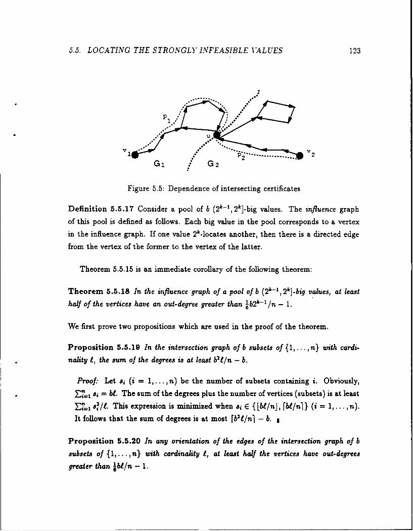
5.5. LOCATING THE STRONGLY INFEASIBLE IALUES 123
I,--2 ...............
Gi : G2
Figure 5.5: Dependence of intersecting certificates
Definition 5.5.17 Consider a pool of b (2 k-1, 2k]-big values. The influence graph
of this pool is defined as follows. Each big value in the pool corresponds to a vertex
in the influence graph. If one value 2k-locates another, then there is a directed edge
from the vertex of the former to the vertex of the latter.
Theorem 5.5.15 is an immediate corollary of the following theorem:
Theorem 5.5.18 In the influence graph of a pool of b (2 k -1, 2k]-big values, at least
half of the vertices have an out-degree greater than lb2 - /n - 1.
We first prove two propositions which are used in the proof of the theorem.
Proposition 5.5.19 In the intersection graph of b subsets of .1,... ,n} with cardi-
nality 1, the sum of the degrees is at least b21t/n - b.
Proof. Let s (i = 1,... ,n) be the number of subsets containing i. Obviously,
E'I si = bt. The sum of the degrees plus the number of vertices (subsets) is at least
E&= s/I. This expression is minimized when si E { bt/nj, fbi/ni } (i = 1,... ,n).
It follows that the sum of degrees is at most rb21/nl - b. ,
Proposition 5.5.20 In any orientation of the edges of the intersection graph of b
subsets of {1,... , n} with cardinality t, at least half the vertices have out-degrees
greater than !b/n - 1.
124 CHAPTER 5. SYSTEMS WITH TWO IARIABLES PER INEQUALITY
Proof: It follows from Proposition 5.5.19 that the sum of out-degrees (i.e.. the total
number of edges) in any subgraph induced by b' vertices is at least 1(b"2 i/n - b).
Suppose, to the contrary, that there exists a subset U of cardinality JUI = V b/2
where the out-degree of each vertex is less than or equal to lbl/n - 1. The total
number of edges (which is the same as the sum of out-degrees) in the subgraph
induced by these vertices is 1 1'2 /n - b', hence a contradiction since it is less that1 - b')..
Proof of Theorem 5.5.18: The cardinality of a certificate of a (2' -1, 2k]-big
value is greater than or equal to I = 2 k-1 . It follows from Proposition 5.5.16 that
if two big values have intersecting certificates, then in the influence graph there is
an edge between the corresponding vertices. Hence, the influence graph contains
an intersection graph of b subsets of {1,..., n} of cardinality 1. Thus, the proof
follows from Proposition 5.5.20. 1
5.5.5 Estimating the number of big values
In this subsection we prove the following proposition:
Proposition 5.5.21 An estimate r' such that 1/2 < r'/r < 2 with probability at
least 1/2, can be found using O((log log n)2 ) "reveal" operations.
The problem of computing an estimate can be stated in the following terms. We
are given a collection of ft stones, where r of them axe radioactive. The number
* is not known. We are equipped with a primitive gauge that when exposed to
a set of stones can determine if at least one of them is radioactive (i.e., "reveal"
operation). A good estimate to the number of radioactive stones is a number r' such
that 1/2 < r'/r < 2. The goal is to compute a good estimate which is correct with
probability at least 1/2, by using at most O((log log )2). gauge readings. We first
give some useful propositions.
5.5. LOCATING THE STRONGLY INFEASIBLE IALUES 125
Proposition 5.5.22 Denote by po(s) the probability that a sample (with returns) of
size s contains no radioactive stones and let c - rs/h. Under these conditions, (i)
po(s) < e- c, and (ii) if r/h < 0.5, po(s) > 4- c.
Proof:S C
It follows that po(s) < e-c and if r/fi < 0.5, Po > 4'. u
Corollary 5.5.23 Suppose po(s) is known. We can conclude as follows:
i. If 0.0625 < po(s) < 0.6, then 1/2 < c < 2.
ii. If 0.0725 < po(s) < 0.59, then 0.53 < c < 1.89.
iii. If po(s) < 0.0825, then c > 1.8.
iv. If po(s) >_ 0.58, then c < 0.544.
Proposition 5.5.24 Let B' be the r.v. which corresponds to the number of non-
radioactive samples out of B = 5000 log log fil random samples of size s.
Prob{IB'/B- po(s)I > 0.01} < 1/(2[logloghl)
Proof: B' is the number of succeb-ses of B Bernoulli trials with success proba-
bility po(s), and hence, has a binomial distribution. Therefore B' has expected
value po(s)B and variance Bpo(s)(1 - po(s)) (see [23] for background). It fol-
lows from Chebyshev inequality that Prob {IB' - po(s)BI > 0.01B} < 2500BIB' =
2500/B = 1/(2 [log logfil ). A smaller constant can be achieved by using the normal
approximation [23].
Denote by po,(s) the r.v. B'/B, and by p'(s) a value of ph(s).
We now describe the algorithm that computes the estimate r-. The algorithm is
based on performing a binary search on the [log ftJ possible estimate values 21, 22,
24 , ...- , 2 log tJ.
126 CHAPTER 5. SYSTEMS WITH TWO VARIABLES PER INEQUALITY
Algorithm 5.5.25 !Compute an estimate]
i. If p'( 2 ) < 0.35, stop and return the estimate r' = 2 L""- .
ii. Initialize a = 1, b = [log fij. Repeat the following until a =b:
iii. Set j = (a + b)/21, and s = 2j .
" If 0.0725 < pg(s) < 0.59, stop and return the estimate r = fi/s.
* If p'(s) < 0.0725, set b = j and go to step iii.
*If p'(s) > 0.59, set a =jand go to step iii.
We show that with probability at least 0.5, 1/2 < r-/r < 2. Consider the first
step. If r > h/2, po(2 ) < 1/4. Hence, Prob{p;(2) < 0.35} < 1/loglog fi. If r <
fi/4, po( 2 ) _ 9/16. Hence, Prob{p'(2) >_ 0.47} < 1/loglogfi. It follows that if
r > h/2, the algorithm stops with the correct estimate with probability at least
1 - 1/(2plog log f1). If r < h/4 the probability that the algorithm stops with an
incorrect estimate is smaller than 1/(2 [og log hi ).
The algorithm performs log log t iterations. Each iteration terminates with further
restriction of the set a, a + 1,... , b. Consider a single iteration. It follows from
Corollaxy 5.5.23 and Proposition 5.5.24 that if at the beginning of the iteration, one of
the values 2 , 2*+,... , 2b is a good estimate, then with probability (1-1/(2 [log log fi)this is still the case when the iteration ends.
Suppose log log ft > 2. The probability that when the algorithm terminates 2 is
a good estimate is at least
(1- 1/(2 Dog logfij))5"° 'mfl > 0.5
The algorithm performs O(log log fi) iterations, where each iteration computes an
appropriate value of p . Each iteration requires O(log log h) "gauge readings" (see
Proposition 5.5.24). Hence, the total number of "gauge readings" performed by the
algorithm is O((log log i)').
5.6. LOCATING WEAKLY INFEASIBLE AND FEASIBLE VALUES 127
5.6 Locating a pool of weakly infeasible values
and feasible values
In this section we present an algorithm which asserts the following:
Theorem 5.6.1 Problem 5.3.6, where the values j (i E I) are guaranteed to be
either feasible or weakly infeasible, can be solved (i) sequentially, in 0(mnlog2 n)
expected time, and (ii) on a CRCW PRAM, in 0(n log 2 n) expected time, using 0(m)
processors.
The following is a key property of feasible and weakly infeasible values:
Proposition 5.6.2 Let j and 4 be feasible or weakly infeasible values of xi and xj,
respectively. If there exists a path p from vi E {j, Vj} to vi E {v, i} such that fp(j)
is tighter than i at the vertex vi, there exist such a simple path p'.
Proof: We assume that vj = Uj, vi = :Ui (the proof for the other cases is similar).
Consider the path p from vi to vi. Suppose a vertex u occurs more than once on
p. Consider two of the occurrences of u. Let p = pip2ps, where p, is the prefix
of p until the first occurrence and p3 is the suffix of p starting from the secondoccurrence of u. If f,p 2 (j) is not tighter than f, (4) at i, the path p' = P3' is
at least as tight as p. Consider iterating the above process. It follows that there
exist a path P from vj to vi which is at least as tight as p with respect to xj = 4,and when a vertex appears more than once, the value at subsequent occurrences is
always tighter. We claim that each vertex may occur at most once in P. Assume
the contrary, and consider the first cycle c along P. Let u be the vertex where c
starts and ends, and let p' = pic be the corresponding prefix of p. It follows from
Proposition 5.2.16 that either f, (4j) is infeasible at u, or fp, (j) is consistent at u.
If fp, (4) is infeasible, p' is a closed certificate for [-oo, 4] with respect to zj and we
get a contradiction to the assumption that j is not strongly infeasible. Otherwise,
&4 (j) is consistent at u. It follows that for every prefix P2 of P which contains p1
and ends at a vertex u', the value f, (j) is consistent at u'. Consider the last cycle
128 CHAPTER 5. SYSTEMS WI7TH TWO VARIABLES PER INEQUALITY
c' along P, and let p' = c'p3 be the corresponding suffix of P. It follows that p' is a
closed certificate for [(i, ool at vi. This is a contradiction to j not being strongly
infeasible. *
We present two procedures which are subroutines of the algorithm for locating a
pool. The first procedure is applied to a subset of the values and returns a partial
solution. The second procedure extends a partial solution as much as possible without
restricting the feasible region further. We discuss the first procedure in detail. The
input is a subset of values Ci (i E I'), where I' C I. The procedure determines
intervals Ji (i E I"), where I" C I' is a subset of the values in the input set. The
intervals Ji (i E I") constitute a partial solution for Problem 5.3.6, that is, there exist
a set of intervals Ji (i E I \ I") such that J1 (i E I) is a solution of Problem 5.3.6.
Algorithm 5.6.3 [Find a partial solution]
i. Initialize the values at the vertices of G as follows:
Y = = i (i E I'), Y = b,, x- = a1 (i V I'),
ii. Apply 2n push phases.
iii. For i E I' do as follows:
" If 6i = Yz = x, set Ji= {jj.
* If j = Yi < -, set Jd = [, oo].
" If fi = & > Yj, set Ji = [ -00, fi].
* Otherwise, Ji is not determined.
Let I"c I' be the set of all i E I' for which J7 is determined. For i E I" do:
Denote by F" the feasible region (1 < i < n) prior to applying Algorithm 5.6.3.
Consider an application of the algorithm. We show that if F- # 0 then the system re-
mains feasible, that is, F # 0. The following proposition proves a necessary condition
for correctness: If F" # 0, then for all i E I", F" f {nz z E Ji} #0
5.6. LOCATING WEAKLY INFEASIBLE AND FEASIBLE 1:ALUES 129
Proposition 5.6.4 Suppose . i = j (resp., j = ) is weakly infeasible. There exist
a simple path p from v to fi (resp., iY, to - ), such that fp( i) < i (resp., f() > ,).
Proof: It suffices to prove the existence of a not necessarily simple path p with
the above properties. The existence of a simple path would follow from Propo-
sition 5.6.2. We assume z i = is weakly infeasible (the other case is proved
similarly). There exist 1 < j < n and two simple paths emanating from v-, p, to
vY and P2 to vj such that fp,(4j) < fm (4j). Consider the path p = pip21 from v. to
Vi. We claim that fp(4i) < 4i. To prove the claim note that fM() = f4-1 ofp (4i).
Since the end vertices of p-' both lie in i, the function f.-' is monotone increasing.
Hence,' f-' of, (,) < f, o f42 (40 = 4i- |
We show that the intervals Ji (i E I") constitute a partial solution:
Proposition 5.6.5 F = F- f {zn AiEI, zi E Ji} # 0.
Proof: It follows from Proposition 5.6.4 that Ji is feasible for all i E I". It follows
from Proposition 5.2.11 part iii that it suffices to show that for every pair {i,j} E I",
F" fl {ni E Ji, zx E Jj} # 0. The latter follows from Corollary 5.2.10. *
We discuss the procedure which extends a partial solution. Suppose we applied
Algorithm 5.6.3 and as a result, for i E I", we updated the intervals Si and determined
Ji. The following algorithm may determine the interval Ji for some additional values
i E I \ I".
Algorithm 5.6.6 [Extend a partial solution]
i. Initialize the values at the vertices of G as follows. x. = ai and Wi = bi (i E I).
ii. Apply 2n push phases.
iii. For i E I \ I' conclude as follows:
" If ri :_ 4j, set Ji = {-o o, }.
SIf z 4,setJi =f4,oo.
130 CHAPTER 5. SYSTEMS WITH TWO V-ARIABLES PER INEQUALITY
Let I" be the set of E I \ ,' such that Ji was determined.
For i E I" do: Si,- S r Ji.
Remark 5.6.7 Proposition 5.2.5 asserts that the feasible region is not changed by
the updates of the intervals Si done by Algorithm 5.6.6. In particular, if the feasible
region was non empty prior to applying the algorithm it remains non empty.
5.6.1 The algorithm
The following algorithm considers feasible and weakly infeasible values fi (i E I), and
solves Problem 5.3.6 for these values. The solution consists of a set of intervals Ji
(i E I). The algorithm performs iterations, where in each iteration some intervals
Ji (i E P' C I) are determined. The intervals Ji (i E I') are incorporated into the
system, we set I +- I \ I', and the problem is reduced to locating the values , (i E I).
Algorithm 5.6.8 [Locate a pool]
i. Repeat the following until I = 0.
ii. For I = 1,2,4,... , 2[LSnJ, execute steps iii-v:
iii. Choose (with returns) I random elements from I. Let I' C I be the set of
chosen elements.
iv. Apply Algorithm 5.6.3 to I'. The algorithm determines J for i E I" C I'.
v. Apply Algorithm 5.6.6 and determine J for additional values 1 E I. Set I
I{" u i}.
It follows from Proposition 5.6.5 and Remark 5.6.7 that if the problem was feasible, it
remains feasible in any point during the execution of the algorithm, hence, when the
algorithm terminates, the intervals Ji (i E I) constitute a solution for Problem 5.3.6.
5.6. LOCATING WEAKLY INFEASIBLE AND FEASIBLE VALUES 131
5.6.2 Complexity
For values j (i E I), consider a solution for Problem 5.3.6, that is, intervals Ji (i E I)
such that Ji E {[-oo, Ci, [Ci, oc]} and XiEJ, r2 0.We designate vertices vi (i E 1) according to the choice of intervals Ji (i E I): If
Ji = [- 00, i] v, = U,. If J = [ j, oo], v, - .
We define a relation on the set I, with respect to the solution Ji (i E I):
Definition 5.6.9 Let i E I, j E I be two elements.
i. We say that j locates i if there exist a path p from vi to vi such that fp(4) is
at least as tight as Ci on vi.
ii. We say that i interferes with j if there exists a path p from vi-1 to vi 1 such
that fp( j) is tighter than 4i on vj "1.
iii. We define the relation -< on I as follows. j - i if and only if i interferes withj.
(Note that when i $ j, i locates j if and only if j interferes with i.)
iv. For an element i E I, denote by pred(i) = {j E Ili :_ i} the set of elements
that locate i, and by succ(i) = {j E Ii >- i} the set of elements which interfere
with i.
The following is a corollary of Proposition 5.6.2:
Corollary 5.6.10 If a path p as in Definition 5.6.9 parts i and ii ezists, then there
must ezist a simple path with the same properties.
The following proposition relates the locate and interfere relations to the algo-
rithms presented earlier. The proof follows from Corollary 5.6.10.
Proposition 5.6.11 Let i E I, j E J be two elements.
i. Suppose that j locates i. If S C Ji, then an application of Algorithm 5.6.6
would determine Ji.
132 CHAPTER 5. SYSTEMS ITH TWO VARIABLES PER INEQUALITY
ii. Suppose that i interferes with j. Consider an application of Algorithm 5.6.3
where {i, j} C I'. The interval Jj will not be determined as a result of such a
run. Moreover, if j E ', the interval Jj is determined in this run if and only if
for all values i E I', i does not interfere with j.
We characterize the values located in an iteration of Algorithm 5.6.8, in terms of
pred and succ:
Corollary 5.6.12 Consider an execution of steps iv-v. An interval Jk (for k E I) is
determined as a result if and only if pred(k) nl I' # 0 and succ(k) nI' = 0.
Proposition 5.6.13 The relation -< is a partial order on 1.
Proof: The transitivity of -< is immediate. We need to show that -< has no cycles.
If there is a cycle, it follows from the transitivity that for some j E I, j interferes
with j. The path p is in this case a simple cycle which constitutes a closed certificate
for j. This contradicts the assumption that 4j is not strongly infeasible. 1
Note that each iteration of steps iii-v results in determining at least one interval,
and therefore, the algorithm terminates within O(n) iterations. In order to prove
Theorem 5.6.1, however, we need to show that the expected number of iterations is
only O(log2 n). We first discuss the chances of an interval Ji (i E I) to be determined
in an iteration:
Proposition 5.6.14 Consider an execution of steps iii-v. If an element i E I is such
that I succ(i)I = 0, then Ji is determined with probability at least po, where po > 0
is some constant, at the steps where I > III/Ipred(i)l. Otherwise, if Ipred(i)l >
I succ(i)1/3, then Ji is determined with probability at least po at the step where
III_ I 21II succ(i)I - - I succ(i)I
5.6. LOCATING WEAKLY INFEASIBLE AND FEASIBLE VALUES 133
Proof: We prove the part where 1 succ(i)i > 0. The first part is similar and simpler.
It follows from Corollary 5.6.12 that Ji is determined with probability
P= Prob{pred(i)nI'# 0 A succ(i)fnI'=0} .
We need to show that there exist a constant po such that P > p0. Since the sets
succ(i) and pred(i) are disjoint, it suffices to show that
P1 = Prob {pred(i) n I' # 0} > pi, and P2 = Prob {succ(i) I' = 0} > P2,
for some constants P, > 0, P2 > 0.
Consider I as above. It follows that P2 > 0.06 and P1 _> 0.28. *
Proof of Theorem 5.6.1: Algorithm 5.6.8 terminates with a correct solu-
tion. We claim that the expected number of iterations of step ii is 0(log n). Each
execution of step ii amounts to 0(log n) calls to Algorithms 5.6.3 and 5.6.6, and
hence, Algorithm 5.6.8 amounts to an expected number of 0(log2 n) applications of
Algorithms 5.6.3 and 5.6.6. Recall that Algorithms 5.6.3 and 5.6.6 run sequentially,
in 0(mn) time, and on a CRCW PRAM, in 0(n) time using 0(m) processors.
It follows that the expected running time of Algorithm 5.6.8 is as stated in the
theorem. What remains is to prove the claim. Consider the quantity
a(I) = If pred(i)l = III + , I succ(i)l
Initially, a < n2 . It suffices to show that an execution of step ii reduces a by at
least a/7, with probability at least 1/2. Ifs < 7111/4,
E I pred(i)I > 9/7
Otherwise, if a > 7111/4, we have Eg Isucc(i) I _ 3 Fi~r I pred(i)1/7, and hence,
F I pred(i)l > 2s/7.
{i:I pred()I> I succ(i)I/3)
The proof follows from Proposition 5.6.14. *
134 CHAPTER 5. SYSTEMS W47TH TWO VARIABLES PER INEQUALITY
5.7 Monotone systems
Consider the following two operations on vectors in Rn:
m y " = (max{X1 ,yi},...,max{x,.,y.})" (the join of x and y)
x A y = (min{ ,yl},...,min{fX,y,4}) T (the meet of x and y)
Consider a TVPI system as in Definition 5.1.1, where the matrix A T (resp., -AT)
is a pre-Leontief matrix, that is, each row of A contains at most one positive (resp.,
negative) entry. The set of solutions of such a system constitutes a semilattice rel-
ative to the V (resp., A) operation (see Cottle and Veinott [15]). It follows that if
all the variables are bounded from above (resp., below), there exists a solution where
all the variables are maximized (resp., minimized) simultaneously, hence, the vec-
tor z (resp., z rai ) is feasible. Also, the associated graph of such a system (see
Definition 5.2.1) does not contain edges from V to V (resp., from V to V).
A TVPI system where the two non-zero coefficients in each inequality have op-
posite signs (equivalently, both AT and -AT are pre-Leontief) is called monotone.
The set of solutions of monotone systems constitutes a lattice relative to the V and
A operations. Note that the converse is also true: if a polyhedral set constitutes
a lattice relative to the V and A operations, then it can be represented as the set
of solutions of some monotone system. The converse is a direct consequence of the
following result due to Veinott [61]: a polyhedral set is a semilattice relative to the
V (resp., A) operation if and only if it constitutes the set of solutions of some inear
system Am < b (resp., A > b), where the matrix AT (resp., -AT) is pre-Leontief.
Consider, for example, the non-monotone system in Figure 5.6. The points (5, 1) and
(3,4) are feasible, but the point (5, 1) A (3,4) = (3,1) is not. Monotone systems are
related to generalized network flow problems: the linear programming dual of the un-
capacitated generalized transshipment problem is monotone. In Chapter 6 we present
algorithms for generalized network flow problem that exploit this relationship.
The algorithms presented here for solving the feasibility of TVPI systems can
be adapted to find the vectors r,in zI for monotone systems. Note that in the
associated graph of a monotone system there are no edges passing between the two
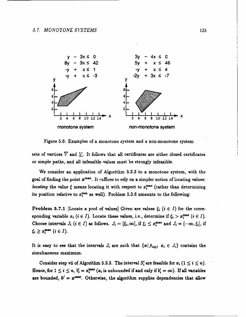
5.7. MONOTONE SYSTEMS 135
y - 3x< 0 3y - 4x-O 08y - 3x- 42 5y + x < 46-y + x:5 1 -y + x -< 4-y + x< -3 -2y + 3x 5 -7
1 18 - 8 -
6 64 -4 -
2- 2
2 4 6 8 0 12 14 2 4 6 8 10 12 14
monotone system non-monotone system
Figure 5.6: Examples of a monotone system and a non-monotone system
sets of vertices V and V. It follows that all certificates are either closed certificates
or simple paths, and all infeasible values must be strongly infeasible.
We consider an application of Algorithm 5.3.3 to a monotone system, with the
goal of finding the point w' . It ruffices to rely on a simpler notion of locating values:
locating the value means locating it with respect to z, = (rather than determining
its position relative to ;? as well). Problem 5.3.6 amounts to the following:
Problem 5.7.1 [Locate a pool of values] Given are values i (i E I) for the corre-
sponding variable xi (i E I). Locate these values, i.e., determine if j > !n'= (i E I).
Choose intervals Ji (i E I) as follows. J, = [ , oo], if e1 < z and J = [-oo,], if
_> (iEI).
It is easy to see that the intervals Yi are such that {zI Aier zi E Ji} contains the
simultaneous maximum.
Consider step vii of Algorithm 5.3.3. The interval Sf are feasible for zi (1 < i < n).
Hence, for 1 < i <n b = z (zi is unbounded if and only if b = oo). If all variables
are bounded, b' = zn2. Otherwise, the algorithm supplies dependencies that allow
136 CHAPTER 5. SYSTEMS WITH TWO 4PIABLES PER INEQUALITY
us to compute feasible solutions when we determine some variables and maximize
others.
Remark 5.7.2 An algorithm which computes x" ' (resp., x' n) for feasible mono-
tone systems can be applied to compute xmax (resp., xr in) for TVPI systems where
the matrix AT (resp., -AT) is pre-Leontief. Consider a system Az < b where at
most one of the two nonzero coefficients in each row is positive. Obtain a monotone
system A'z < b' by omitting all rows of A where there are two negative entries.
Compute the vector y which maximizes all variables in the resulting monotone sys-
tem. If the original system Ax < b is feasible, y is the vector which maximizes all
variables.
5.8 Concluding remarks
In this chapter we considered systems of linear inequalities, where each inequality has
at most two nonzero coefficients (TVPI systems). We presented algorithms which
solve the feasibility problem, that is, either find a point which satisfies all the in-
equalities or conclude that no such point exists. We gave a 6 (mn2) deterministic
algorithm and a 6(n' + mn) expected time randomized algorithm. The complexities
of the respective parallel implementations are: 0(n) time using O(mn) processors,
and 6(n) expected time using O(n 2 + M) processors. Although the analysis of these
algorithms seems quiet lengthy, the algorithms themselves are simple. The underlying
computation amounts the basic Bellman-Ford and Floyd-Warshall [13] shortest path
algorithms where only data structures are used.
We give some comments and suggestions for further research:
The time complexity of the randomized algorithm involves many logarithmic fac-
tors (log" n). We believe that a more careful analysis may eliminate some of these
factors. Another obvious question is whether the 6(n' + inn) bound can be achieved
deterministically.
5.8. CONCLUDING REMARKS 137
We discuss the possibility of improving over a 6(n' - inn) bound. The 0(n 3 )
factor results from the all-pairs shortest part Floyd-Warshall computation and is in-
herent from our basic framework. A different approach, however, may yield a O(mn)
algorithm.
The feasibility problem of monotone systems includes as a very special case the prob-
lem of detecting existence of negative-weight directed cycles in a graph with n nodes,
m edges, and real weights associated with the edges. The best known bound for de-
tecting negative weight cycles is O(mn), and hence, we believe it is improbable that a
5(ran) algorithm exists for solving TVPI systems. We sketch the reduction. Consider
a weighted graph G = (171 E, w), where w : E -+ R. The corresponding monotone
system is as follows. For each node v E V assign a variable z,. For each edge
e = (u, v) E E assign the inequality z,, - z. < w(e). It follows from Proposition 5.2.9
that G contains a negative weight cycle if and only if the system is infeasible.
Our algorithms solve the feasibility problem of TVPI systems. They can be
adapted, however, to (i) find a solution which maximizes a specific variable (ii) and
find the lexicographic maximum. Questions that remain open regard finding an op-
timal solution relative to an arbitrary linear objective function. It is not known
whether a strongly polynomial time algorithm exists for the problem, or whether we
can achieve a time bound which is better than specializations of existing general LP
algorithms. A partial result is due to Cosares [14] who showed that when the objective
function has a fixed number of nonzero entries, the problem can be solved in strongly
polynomial time bounds. The degree of the polynomial, however, grows linearly with
the number of nonzero entries.
We discuss the parallel complexity of solving TVPI systems. Lueker, Megiddo,
and Ramachandran [43] showed that the problem of finding an optimal solution rela-
tive to a general objective function is P-complete. It is not known, however, whether
the feasibility problem is P-complete. The algorithms presented in this chapter have
a parallel running time of 6(n). These are the best known parallel time bound
achievable by a polynomial number of processors. Lueker, Megiddo, and Ramachan-
dran [43] gave an algorithm for the problem which runs in polylogarithmic time, but
uses n° 0kg- ) processors.
Chapter 6
Algorithms for generalized
network flows
A generalized network is a digraph G = (V, E) given together with positive flow
multipliers a. (e E E) associated with the edges. The multiplier a. (e E E) is
interpreted as a gain factor (when a. > 1) or a loss factor (when a. < 1) of flow along
the edge e; when z, units of flow "enter" the edge e, a6z. units "leave". Generalized
network flows are also known in the literature as flows with losses and gains. They
can be used to model many situations that arise in financial analysis [25, 26, 42].
The uncapacitated generalized transshipment problem (UGT) is defined on a gen-
eralized network, where costs are given for the edges and supplies or demands are
given for the nodes. The goal is to find a flow of minimum cost, which satisfies the
supplies/demands. Adler and Cosares [1] gave an algorithm for solving restricted
instances of UGT where there are many sources and no sinks. Their algorithm is
based on a solution for the linear programming dual, which turns out to be a mono-
tone TVPI system, and hence, the results of Chapter 5 imply better time bounds for
restricted UGT.
In the generalized circulation problem (GC) we consider a generalized network
where demands (nonnegative numbers) are given for the nodes and capacity con-
straints are given for the edges. The goal is to find a feasible flow which maximizes
138
139
the proportion of satisfied demands. Goldberg, Plotkin, and Tardos [26' presented
an algorithm for the seemingly more general capacitated generalized transshipment
problem without costs. Their algorithm is based on solving an instance of GC which
has a single demand node (the source) and performs O(mn) additional computation.
We present a scheme for solving generalized circulation problems by iteratively relax-
ing the capacity constraints, solving an instance of UGT on the same network with
costs which "capture" the capacities, scaling the flow to a feasible one, and replacing
the capacities by the residual capacities relative to this flow.
This scheme introduces a general method of approximating a solution to linear
programming problems in the following situation. For given matrices A E R" ',
U E Rlexm and vectors b E R", d E R', where U, d have nonnegative entries,
maximize t subject to: (i) Am = tb, x > 0, and (ii) Um < d. Condition (ii) can be
viewed as generalized capacity constraints. We assume that for c > 0, it is "easy"
to minimize cTx subject to Aam = b, x > 0. Denote by t the maximal value of the
objective function. We will show that a feasible solution 2' E R, t' E R such that
t' > t1/ can be found by solving a single instance of the "easy" problem.
Consider the generalized circulation problem with the relaxed goal of computing
a flow which satisfies a proportion of the demands which approximates to a constant
factor the best achievable proportion. For the relaxed problem, the scheme described
above yields a strongly polynomial time algorithm, which is also the fastest known
(on some ranges) algorithm. This scheme also yields an algorithm for obtaining an
optimal solution, which is the fastest known on some ranges.
In Section 6.1 we define the UGT problem and review the Adler and Cosares [1]
algorithm. In Section 6.2 we introduce the approximation algorithm and apply it to
the generalized circulation problem. In Section 6.3 we introduce bidirected gener-
alized networks and discuss the UGT and generalized circulation problems on these
networks. Section 6.4 contains concluding remarks.
Note that for instances of the problems mentioned above we need to consider cases
where m = w(n 2 ). The algorithms presented here handle multiple edges within the
stated time bounds.
140 CHAPTER 6. ALGORITHMS FOR GENERALIZED NETWORK FLOWS
6.1 Generalized transshipment problem
Problem 6.1.1 [Uncapacitated Generalized Transshipment (UGT)J
Given are a generalized network G = (1, E), edge-costs c. (e E E), and supplies (or
demands) bi (1 < i < n) for the nodes. Find a nonnegative flow function z = (z.)
such that
for every i, E aexe - E e =bj,eEin(i) eEout(i)
so that the cost &eEE cxz is minimized.
When bi > 0 (resp., bi < 0), we refer to the i'th node as a source (resp., sink). The
linear programming dual has the following form. Find values for ri,... , r, which
maximize F,!' biri, subject to the monotone inequalities
for all e E E: ri - aerj : c, where e is from i toj.
In this section we consider restricted instances of UGT where there are either
only sources (b > 0) or only sinks (b < 0). Adler and Cosares [1] proposed a
scheme for solving a subset of the LP problems where each variable appears in at
most two inequalities. In particular, the scheme is applicable to restricted UGT
instances. They showed that these instances can be solved using a single application
of Megiddo's algorithm for TVPI systems [46]. An application of the faster algorithms
for TVPI systems presented in Chapter 5 can be used instead. Hence, restricted
UGT instances can be solved deterministically in 0 (mn2(log m + log 2 n)) time, and
in 0 (n3 log n + mn(log m log 3 n + logs n)) expected time.We characterize the problems for which the scheme of [1] is applicable. Consider
an LP problem, 7, of the following form. minimize cT , subject to Am = b, z > 0,
where A E Rn"Xf contains at most two non zero entries in each column. Denote
by m' E R/ the optimal solution of 'P. Note that the LP dual of 'P amounts to
optimizing an arbitrary objective function subject to a TVPI system. The scheme
of [1] is applicable to 7 if Z" = i:b#o x[', where m(') > 0 maximizes cTz subject to
Am = bie i .
6.2. GENERALIZED CIRCULATION 141
We sketch the ideas used in their scheme. Denote by S the TVPI constraints
ATWr < c. Let ir~" (resp., r1X) be the minimum (resp., maximum) value of r,i
subject to S.
If 7rTlx = o (resp., r n = -co), then P is feasible only if b, < 0 (resp., b, > 0).
If bi # 0, a vector x(i) as defined above can be constructed from a minimal subset of
constraints from S which implies (i) ri < :5 7m if bi > 0, or (ii) 7ri > r if b < 0. The
edges which correspond to such a minimal system comprise a generalized augmenting
path [29] of flow to the i'th node (i.e., a flow generating cycle and a path from a node
on the cycle to the i'th node). The vector x(i) is obtained by considering the flow
values at the edges when pushing flow along this augmenting path.
It is easy to see that the scheme of [1] is applicable to restricted UGT instances.
Consider a UGT instances where b > 0 (the arguments are similar for b < 0). The
constraints in S are monotone, and therefore, by a single application of the algorithm
of Chapter 5 we determine r" for i = 1,..., n (see Section 5.7). If i' < oo, the
algorithm also computes a minimal subset of constraints from S which asserts that
7 < rr. The vector x(i) can be constructed by using this information. Conclude
as follows. If rf = o and bi > 0, the UGT system is not feasible. Otherwise,
X = Ei:,>o X(i) is a solution.
6.2 Generalized circulation
Definition 6.2.1 Consider a generalized network G = (V, E), where demands bi > 0
(1 < i < n) are given for the nodes and capacities ci _> 0 (possibly cji = oo) are
given for the the edges.
i. A generalized flow is a flow function z = (z.) (z. _ 0) which satisfies the
following. There exist a scalar i(z) -i such that for every 1 < i < n,
£,ein(i) aez - E1 Eout(, Ze = lbi (the flow z satisfies a proportion i(x) of the
demands).
ii. A generalized flow is feasible if z, _< c. for all edges.
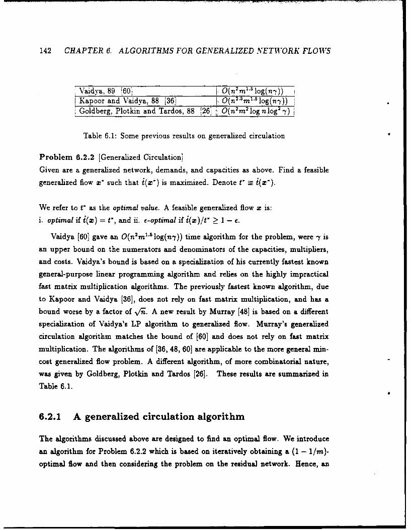
142 CHAPTER 6. ALGORITHMS FOR GENERALIZED NETWORK FLOWS
Vaidya, 89 j601 I O(n 2M 1 log(n-y))
Kapoor and Vaidya, 88 [361 O(n"m2'. 5 1g(n'y)) i
Goldberg, Plotkin and Tardos, 88 i26] YO(n2 m 2 ognlog -)
Table 6.1: Some previous results on generalized circulation
Problem 6.2.2 [Generalized Circulation]
Given are a generalized network, demands, and capacities as above. Find a feasible
generalized flow x" such that i(x') is maximized. Denote t' - t(x').
We refer to t' as the optimal value. A feasible generalized flow z is:
i. optimal if i(x) = t, and ii. e-optimal if i()/t" > 1 - e.
Vaidya [60] gave an O(n 2 m' log(n-y)) time algorithm for the problem, were - is
an upper bound on the numerators and denominators of the capacities, multipliers,
and costs. Vaidya's bound is based on a specialization of his currently fastest known
general-purpose linear programming algorithm and relies on the highly impractical
fast matrix multiplication algorithms. The previously fastest known algorithm, due
to Kapoor and Vaidya [36], does not rely on fast matrix multiplication, and has a
bound worse by a factor of V/'n. A new result by Murray [48] is based on a different
specialization of Vaidya's LP algorithm to generalized flow. Murray's generalized
circulation algorithm matches the bound of [60] and does not rely on fast matrix
multiplication. The algorithms of [36, 48, 60] are applicable to the more general min-
cost generalized flow problem. A different algorithm, of more combinatorial nature,
was given by Goldberg, Plotkin and Tardos [26]. These results are summarized in
Table 6.1.
6.2.1 A generalized circulation algorithm
The algorithms discussed above are designed to find an optimal flow. We introduce
an algorithm for Problem 6.2.2 which is based on iteratively obtaining a (1 - 1/r)-
optimal flow and then considering the problem on the residual network. Hence, an
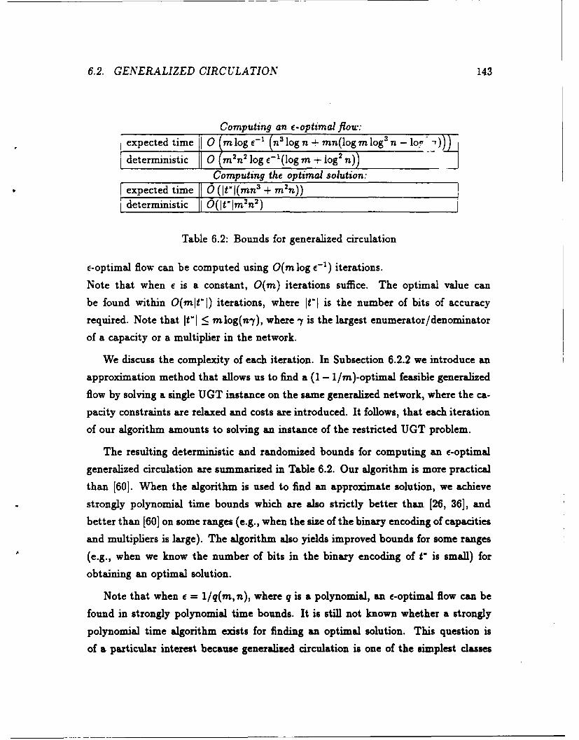
6.2. GENERALIZED CIRCULATION 143
Computing an e-optimal flow:
expected time 0 (m logC -1 (n3 log n + mn(log m log 3n - lo, ')))deterministic 2I 0 n2 logC-1 (log M + log 2 nL)) _
Computing the optimal solution:Fexpected time II0 ( t"(mn 3 + m 2 n))
deterministic IO(t'"m2 n 2 )
Table 6.2: Bounds for generalized circulation
E-optimal flow can be computed using O(m log e-1 ) iterations.
Note that when e is a constant, O(m) iterations suffice. The optimal value can
be found within 0(mlt-I) iterations, where It't is the number of bits of accuracy
required. Note that [t'l < mlog(n-y), where - is the largest enumerator/denominator
of a capacity or a multiplier in the network.
We discuss the complexity of each iteration. In Subsection 6.2.2 we introduce an
approximation method that allows us to find a (1 - 1/m)-optimal feasible generalized
flow by solving a single UGT instance on the same generalized network, where the ca-
pacity constraints are relaxed and costs are introduced. It follows, that each iteration
of our algorithm amounts to solving an instance of the restricted UGT problem.
The resulting deterministic and randomized bounds for computing an e-optimal
generalized circulation are summarized in Table 6.2. Our algorithm is more practical
than [60]. When the algorithm is used to find an approximate solution, we achieve
strongly polynomial time bounds which are also strictly better than [26, 36], and
better than [60] on some ranges (e.g., when the size of the binary encoding of capacities
and multipliers is large). The algorithm also yields improved bounds for some ranges
(e.g., when we know the number of bits in the binary encoding of t is small) for
obtaining an optimal solution.
Note that when e = 1/q(m, n), where q is a polynomial, an e-optimal flow can be
found in strongly polynomial time bounds. It is still not known whether a strongly
polynomial time algorithm exists for finding an optimal solution. This question is
of a particular interest because generalized circulation is one of the simplest classes
144 CHAPTER 6. ALGORITHMS FOR GENERALIZED NETWORK FLOWS
of linear programming problems for which no strongly polynomial algorithms are
known [26, 59]
6.2.2 Obtaining an approximation
Consider linear programming problems of the following form. Given are matrices
A E Rnxin, U E RLX" , and vectors b E R", d E R', where U > 0, d > 0. The goal is
to maximize i, subject to Am = ib, z > 0, and Uz < d. We refer to the constraints
Um < d as generalized capacity constraints. A vector m > 0, such that A: cc b (Ax
is proportional to b) and Uz < d is called feasible. For a feasible vector X, denote
by i(o) the scalar i such that A: = ib. Denote by t- the optimal solution, and by
m' some vector where i(z:) = t. A feasible vector : is e-optimal if i(x)/t" > 1 - C.
Suppose that for 0 < c E R"' it is "easy" to compute a vector m > 0 which
minimizes CTz, subject to A: = b. We refer to problems of this form as uncapacitated
instances. An instance of the original problem is referred to as a capacitated instance.
Note that when the capacitated problem is an instance of generalized circulation, U
is a diagonal matrix with at most m = ]EI rows. The corresponding uncap4,citated
problem is an instance of UGT on the same network, where only demand nodes are
present.
We presents an algorithm for constructing a (1/1)-optimal vector p. The algorithm
amounts to solving a single instance of the uncapacitated problem. Consider the cost
functionI
t=1
It is easy to verify that this function is linear and has the following properties:
i. If z is feasible then p(:) < 1
ii. If z > O, Am c b, and p(z) < 1, then m is feasible.
iii. If p(z') > 0, then p(z') 2 1 (since for some i, Ui.z" = d,).
6.2. GENERALIZED CIRCULATION 145
Consider a vector y > 0, Ay oc b, p(y) = 1 which maximizes i(y). Note that the
vector fy maximizes t(x) for all vectors x > 0 such that p(x) < i and Ax oc b.
In particular i(fy) > tV, and hence, i(y) 2 tI. Such a vector y can be obtained
by normalizing a vector x > 0 which minimizes p(x) subject to Ax = b. Also, y
is feasible and therefore provides the desired approximation. A formal description of
the algorithm follows.
Algorithm 6.2.3 [Compute a (1/1)-optimal vector!
i. Solve the following instance of the uncapacitated problem: Minimize p(x) sub-
ject tox > 0 and Ax = b.
If it is infeasible, then stop and claim that x = 0 is the only feasible vector of
the capacitated instance. Otherwise, let x be the solution.
ii. If p(x) = 0, stop; the vectors rx are feasible for all r > 0, and the capacitated
problem is unbounded.
iii. Otherwise, when p(m) 0 0, compute the largest number r (must be bounded),
such that rUr < d. Claim that rx is (1/1)-optimal.
Correctness: Consider the vector x computed in step i of the algorithm. Note that
x is such that i(x) = 1. Hence, i(rx) = ri(:) = r.
Proposition 6.2.4 p(:) = 0 if and only if the capacitated problem is unbounded.
Proof: Suppose that p(m) = 0. Observe that for all r > 0, p(rx) = 0, and hence,rx is feasible. Also, for all r > 0, i(r:) = r. Hence, the problem is unbounded.
Suppose the problem is unbounded. There exist a vector x such that r: is feasible
for all r > 0. It follows that p(r:) = rp(m) _< 1 for all r > 0. Hence, p(:) = 0. *
The following proposition concludes the correctness proof.
Proposition 6.2.5 If t is bounded, then r > t'/l.
146 CHAPTER 6. ALGORITHMS FOR GENERALIZED NETWORK FLOWS
Proof. For k > 0, denote
R(k) = max{i(y) I p(y) < k, Ay cx by > O} ,and
R'(k) = max{i(y) I p(y) < k,y is feasible}.
Obviously, (i) R and R- are increasing functions, (ii) R > R-, (iii) for every a > 0,
R(ak) = aR(k), and (iv) t < R'(I).
The vector x (computed in step i) is such that R(p(x)) = 1, and hence R(p(rz)) =
r. Since p(x) > 0, Ui.rx = d, for some 1 < i < I. Hence, p(rx) _ 1. It follows
that
t- < R-(t) : R(t) : R(fp(rz)) = erR(p(x)) = ii.
6.3 Bidirected generalized networks
In the previous sections we discussed generalized networks where the flow multipliers
are positive numbers. We refer to the edges in these networks as tail-head edges.
Tail-head edges contribute nonnegative amount of flow at the tail end of the edge
and a proportional nonpositive amount at the head end. In bidirected generalized
networks we allow two additional types of edges: two-head edges and two-tail edges.
The properties of these edge types are shown in Figure 6.1. Note that a 2-tail edge
can be viewed as a tail-head edge with a negative multiplier. Bidi--cted generalized
networks are a generalization of bidirected networks (see [42]). In biderected networks
the multipliers associated with the edges are always unity. Bidirected networks were
first considered by Edmonds [20] who related them to non-bipartite matching theory.
In this section we apply the methods discussed in previous sections to flow problems
on bidirected generalized networks.
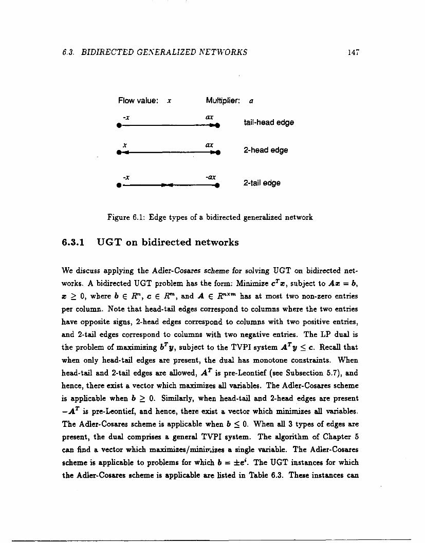
6.3. BIDIRECTED GENERALIZED NETWORKS 147
Flow value: x Multiplier: a
-x ax0 -- tail-head edge
x ax.... _ 2-head edge
-X -ax-- 2-tail edge
Figure 6.1: Edge types of a bidirected generalized network
6.3.1 UGT on bidirected networks
We discuss applying the Adler-Cosares scheme for solving UGT on bidirected net-
works. A bidirected UGT problem has the form: Minimize cT, subject to Ax = b,
x > 0, where b E Rn, c E R'" , and A E Rnx has at most two non-zero entries
per column. Note that head-tail edges correspond to columns where the two entries
have opposite signs, 2-head edges correspond to columns with two positive entries,
and 2-tail edges correspond to columns with two negative entries. The LP dual is
the problem of maximizing bTY, subject to the TVPI system ATy < c. Recall that
when only head-tail edges are present, the dual has monotone constraints. When
head-tail and 2-tail edges are allowed, AT is pre-Leontief (see Subsection 5.7), and
hence, there exist a vector which maximizes all variables. The Adler-Cosares scheme
is applicable when b > 0. Similarly, when head-tail and 2-head edges are present
-A T is pre-Leontief, and hence, there exist a vector which minimizes all variables.
The Adler-Cosares scheme is applicable when b < 0. When all 3 types of edges are
present, the dual comprises a general TVPI system. The algorithm of Chapter 5
can find a vector which maximizes/minirrizes a single variable. The Adler-Cosares
scheme is applicable to problems for which b = ±e'. The UGT instances for which
the Adler-Cosares scheme is applicable are listed in Table 6.3. These instances can
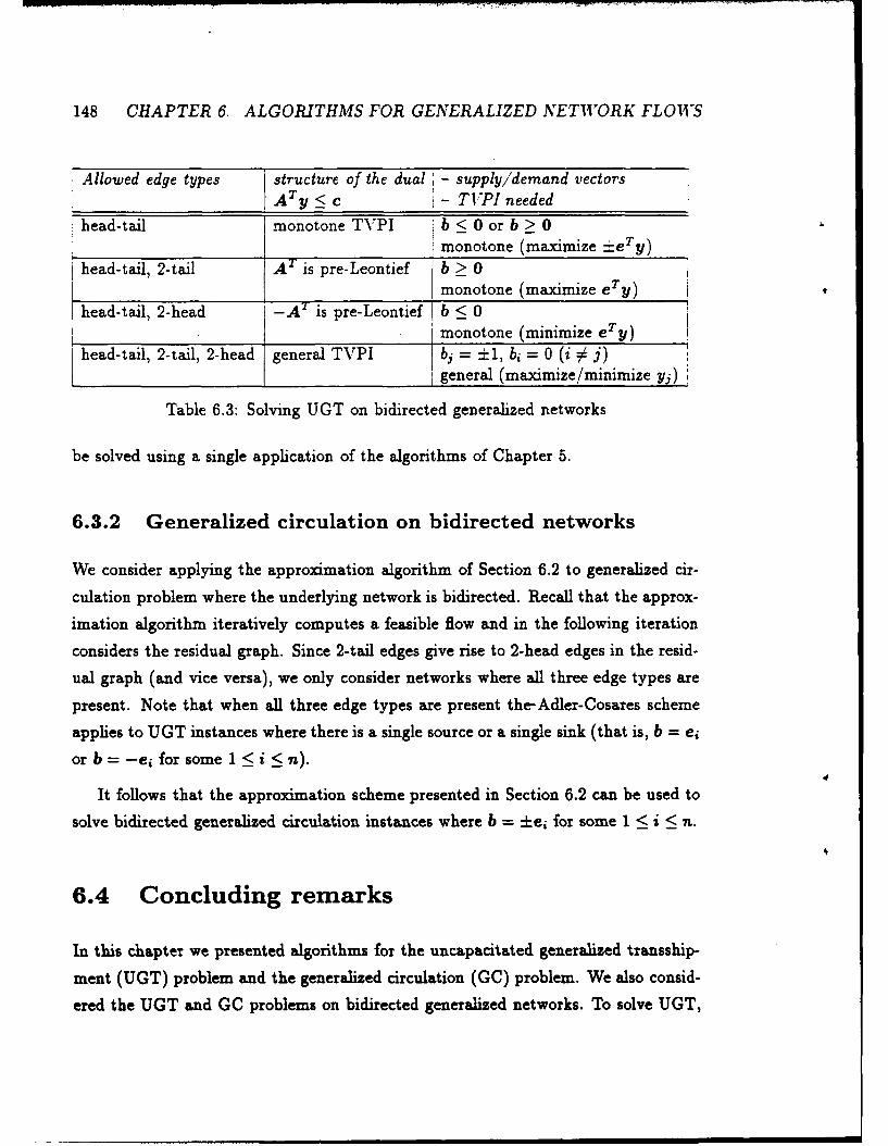
148 CHAPTER 6. ALGORITHMS FOR GENERALIZED NETWORK FLOWS
Allowed edge types structure of the dual - supply/demand vectorsATy K c - TVPI needed
head-tail monotone TVPI b < 0 or b > 0, monotone (maximize -i-eTy)
head-tail, 2-tail A7_ is pre-Leontief b > 0monotone (maximize eT y)
head-tail, 2-head -A' is pre-Leontief b < 0_ _ _ monotone (minimize e y)
head-tail, 2-tail, 2-head general TVPI bj = -1, bi = 0 (i # j)_ general (maximize/minimize yj)
Table 6.3: Solving UGT on bidirected generalized networks
be solved using a single application of the algorithms of Chapter 5.
6.3.2 Generalized circulation on bidirected networks
We consider applying the approximation algorithm of Section 6.2 to generalized cir-
culation problem where the underlying network is bidirected. Recall that the approx-
imation algorithm iteratively computes a feasible flow and in the following iteration
considers the residual graph. Since 2-tail edges give rise to 2-head edges in the resid-
ual graph (and vice versa), we only consider networks where all three edge types are
present. Note that when all three edge types are present the-Adler-Cosares scheme
applies to UGT instances where there is a single source or a single sink (that is, b = ej
orb= -ei forsome 1 <i <n).
It follows that the approximation scheme presented in Section 6.2 can be used to
solve bidirected generalized circulation instances where b = ±ej for some 1 < i < n.
6.4 Concluding remarks
In this chapter we presented algorithms for the uncapacitated generalized transship-
ment (UGT) problem and the generalized circulation (GC) problem. We also consid-
ered the UGT and GC problems on bidirected generalized networks. To solve UGT,
6.4. CONCLUDING REMARKS 149
we combined a scheme by Adler and Cosares 1, which reduces the restricted UGT
problem where either only demand nodes or only supply nodes are present to solving
the LP dual, with the algorithms given in Chapter 5. The combination yielded better
time bounds for restricted UGT instances.
In order to utilize the UGT algorithms for solving the capacitated GC problem,
we introduced an iterative approximation algorithm. In each iteration, we consider
a UGT instance, with costs which "capture" the relaxed capacities. The solution of
this UGT instance yields an approximate solution for the GC instance. The next
iteration considers the residual graph.
We comment on the parallel running times of the algorithms mentioned above.
The parallel complexity of the algorithms of Chapter 5 is 0(n) using 0(mn) processors
for the deterministic bound and O(m + n') processors for the randomized bound.
The algorithms for the restricted UGT instances have the same complexity. The
approximation algorithm for GC runs in t5(mn log e-1) time using 0(mn) processors
for the deterministic bound and O(m + n2) processors for the randomized bound.
A problem which remains open regards the existence of a strongly polynomial for
the unrestricted UGT problem (where many sources and sinks are allowed). The LP
dual of UGT is a monotone system with a general objective function; what brings as
back to an open question from Chapter 5. The following reduction (similar to [52])
demonstrates the difficulty of the problem. An instance of capacitated generalized
transshipment can be reduced in linear time to an instance of UGT with 3m edges
and n + 2m nodes. The reduction is as follows. Consider an instance of generalized
circulation on a network G = (V, E) where d, E R is the supply/demand at v (v E
V), and ae,ue,c. are the multiplier, capacity, and cost, respectively, of the edge e
(e E. E). The corresponding UGT instance G' = (V U W U W', E') preserves the
supplies and demands at the nodes V. Each edge e E E has corresponding two nodes
we E W,w, E W' and three edges in E' which form an undirected path. The node
We has demand u. and w' has supply -u.. Suppose e = (vI, v2), the corresponding
edges are (i) (vi, w) with multiplier 1 and cost c., (ii) (w' , w) with multiplier 1 and
cost 0, and (iii) (w',v 2) with multiplier a, and cost 0.
Chapter 7
Conclusion
In Chapter 2 we presented an NC and strongly polynomial algorithm to detect cycles
in fixed dimensional periodic graphs. This algorithm is based on a strongly polyno-
mial algorithm given in Chapter 3 for the parametric minimum cycle problem with
fixed number of parameters. In Chapter 4 we presented the algorithm of Chapter 3
as a general tool for achieving strongly polynomial time bounds. In Chapter 5 we
gave faster algorithms for linear systems of inequalities, where at most two variables
appear in each inequality. In Chapter 6 we introduced algorithms for some gener-
alized network flow problems which utilize the results of Chapter 5. In particular
we obtained a faster algorithm for approximating the optimal generalized circulation,
which is also the first strongly polynomial algorithm for the problem. The existence of
this approximation algorithm is particularly interesting since it is still open whether
there exist a strongly polynomial algorithm for computing the optimal solution.
These results are interesting in and of themselves, but our work is a step towards
attacking an important open problem of the field: finding a strongly polynomial
algorithm for general linear programming.
150
Bibliography
[1] I. Adler and S. Cosares. Strongly polynomial algorithms for linear programming
problems with special structure. Oper. Res., 1991. To appear.
[2] R. K. Ahuja, J. B. Orlin, and R. E. Tarjan. Improved time bounds for the
maximum flow problem. SIAM J. Comput., 18:939-954, 1989.
[3] B. Aspvall. Efficient algorithms for certain satisfiability and linear programming
problems. PhD thesis, Department of Computer Science, Stanford University,
Stanford, Ca., 1980.
[4] B. Aspvall and Y. Shiloach. A polynomial time algorithm for solving systems of
linear inequlities with two variables per inequality. SIAM J. Comput., 9:827-845,
1980.
[5] K. L. Clarkson. Linear programming in O(n x 32) time. Information Processing
Let., 22:21-27, 1986.
[6] E. Cohen and N. Megiddo. Strongly polynomial and NC algorithms for detecting
cycles in dynamic graphs. In Proc. 21st Annual A CM Symposium on Theory of
Computing, pages 523-534. ACM, 1989.
[7] E. Cohen and N. Megiddo. Maximizing concave functions in fixed dimension.
Technical Report RJ 7656 (71103), IBM Almaden Research Center, San Jose,
CA 95120-6099, August 1990.
151
152 BIBLIOGRAPHY
[8' E. Cohen and N. Megiddo. Recognizing properties of periodic graphs. Technical
Report RJ 7246 (68013), IBM Almaden Research Center, San Jose, CA 95120-
6099, January 1990.
[91 E. Cohen and N. Megiddo. Strongly polynomial time and NC algorithms for
detecting cycles in periodic graphs. Technical Report RJ 7587 (70764), IBM
Almaden Research Center, San Jose, CA 95120-6099, July 1990.
[101 E. Cohen and N. Megiddo. Complexity analysis and algorithms for some flow
problems. In Proc. 2nd ACM-SIAM Symposium on Discrete Algorithms, pages
120-130. ACM-SIAM, 1991.
[11] E. Cohen and N. Megiddo. Improved algorithms for linear inequalities with twovariables per inequality. In Proc. 23rd Annual ACM Symposium on Theory of
Computing, pages 145-155. ACM, 1991.
[12] E. Cohen and N. Megiddo. Recognizing properties of periodic graphs. Applied
Geometry and Discrete Math., The "Victor Klee Festschrift", 1991. To appear.
[13] T. Cormen, C. Leiserson, and R. Rivest. Introduction to algorithms. McGraw-Hill
Book Co., New York, 1990.
[14] S. Cosares. On the complezity of some primal-dual linear programming pairs.PhD thesis, Department of IEOR, University of California, Berkeley, Ca., 1988.
[15] R. W. Cottle and A. F. Veinott Jr. Polyhedral sets having a least element. Math.
Prog., 3:238-249, 1972.
[16] J. B. Dantzig. Linear programming and eztensions. Princeton Univ. Press,
Princeton, NJ, 1962.
[17] E. A. Dinic. Algorithm for solution of a problem of maximum flow in networks
with power estimation. Soviet Math. Dokl., 11:1277-1280, 1970.
[18] D. P. Dobkin, R. J. Lipton, and S. P. Reiss. Linear programming is Log-Space
hard for P. Information Processing Let., 8(2):96-97, 1978.
BIBLIOGRAPHY 153
191 M. E. Dyer. On a multidimensional search technique and its application to the
Euclidean one-center problem. SIAM J. Comput., 15:725-738, 1986.
'201 J. Edmonds. An introduction to matchings. In Engineering Summer Conference.
The Univ. of Michigan, Ann Arbor, 1967. Mimeographed notes.
,21j J. Edmonds and R. M. Karp. Theoretical improvements in algorithmic efficiency
for network flow problems. J. Assoc. Comput. Mach., 19:248-264, 1972.
[22] J. Farkas. Theorie der einfachen ungleichungen. J. Reine und Angewandte Math.,
124:1-27, 1902.
[23] W. Feller. An introduction to probability theory and its applications. John Wiley
& Sons, New York, 1950.
[24] S. Fortune and J. Wyllie. Parallelism in random access machines. In Proc. 10th
Annual ACM Symposium on Theory of Computing, pages 114-118. ACM, 1978.
[25] F. Glover, J. Hultz, D. Klingman, and J. Stunz. Generalized networks: a fun-
damental computer-based planning tool. Management Science, 24(12), August
1978.
[26] A. V. Goldberg, S. K. Plotkin, and t. Tardos. Combinatorial algorithms for
the generalized circulation problem. In Proc. 29th IEEE Annual Symposium on
Foundations of Computer Science, pages 432-443. IEEE, 1988.
[27] A. V. Goldberg and R.E. Tarjan. A new approach to the maximum flow problem.
In Proc. 18th Annual A CM Symposium on Theory of Computing, pages 136-146.
ACM, 1986.
[28] A. V. Goldberg and R.E. Tarjan. Finding minimum cost circulations by succes-
sive approximation. Math. of Oper. Res., 15:430-466, 1990. To appear.
[29] M. Gondran and M. Minoux. Graphs and Algorithms. John Wiley & Sons, New
York, 1984.
154 BIBLIOGRAPHY
[30] B. Gr6tschel, L. Lovasz, and Schrijver A. Geometric algorithms and combinato-
rial optimization Springer-Verlag, New York, 1988.
[31] B. Griinbaum. Convex polytopes. Interscience-Wiley, London, 1967.
[32] D. Hochbaum and J. Naor. Simple and fast algorithms for linear and integer
programs with two variables per inequality. Manuscript, 1991.
[33] K. Iwano. Some problems on doubly periodic infinite graphs. Technical Report
CS-TR-078-87, Princeton University, 1987.
[34] K. Iwano and K. Steiglitz. Testing for cycles in infinite graphs with periodic
structure. In Proc. 19th Annual ACM Symposium on Theory of Computing,
pages 46-53. ACM, 1987.
[35] K. Iwano and K. Steiglitz. Planarity testing of doubly connected periodic infinite
graphs. Networks, 18:205-222, October 1988.
[36] K. Kapoor and P. M. Vaidya. Speeding up Karmarkar's algorithm for multicom-
modity flows. Math. Prog., 1991. To appear.
[37] N. Karmarkar. A new polynomial-time algorithm for linear programming. Com-
binatorica, 4:373-395, 1984.
[38] R. M. Karp. A characterization of the minimum cycle mean in a digraph. Discrete
Mathematics, 23:309-311, 1978.
[39] R. M. Karp, R. E. Miller, and S. Winograd. The organization of computations
for uniform recurrence equations. J. Assoc. Comput. Mach., 14:563-590, 1967.
[40] L. G. Khachiyan. A polynomial algorithm in linear programming. Soviet Math.
Dokl., 20:191-194, 1979.
[41] K. S. Kosaraju and G. F. Sullivan. Detecting cycles in dynamic graphs in poly-
nomial time. In Proc. 2Oth Annual A CM Symposium on Theory of Computing,
pages 398-406. ACM, 1988.
BIBLIOGRAPHY 155
[42' E. L. Lawler. Combinatorial optimization: networks and matroids. Holt. Rein-
hart, and Winston, New York, 1976.
[431 G. S. Lueker, N. Megiddo, and V. Ramachandran. Linear programming with two
variables per inequality in poly log time. SI4M J. Comput., 19(6):1000-1010,
1990.
[441 N. Megiddo. Combinatorial optimization with rational objective functions. Math.
of Oper. Res., 4:414-424, 1979.
[45] N. Megiddo. Applying parallel computation algorithms in the design of serial
algorithms. J. Assoc. Comput. Mach., 30:337-341, 1983.
[46] N. Megiddo. Towards a genuinely polynomial algorithm for linear programming.
SIAM J. Comput., 12:347-353, 1983.
[471 N. Megiddo. Linear programming in linear time when the dimension is fixed. J.
Assoc. Comput. Mach., 31:114-127, 1984.
[48] S. Murray. An interior point conjugate gradient approach to the generalized flow
problem with costs and the multicommodity flow problem dual. Manuscript,
1991.
[49] C. G. Nelson. An n °0(ogn) algorithm for the two-variable-per-constraint linear
programming satisfiability problem. Technical Report AIM-319, Stanford Uni-
versity, 1978.
[50] C. H. Norton, S. A. Plotkin, and t. Tardos. Using separation algorithms in fixed
dimension. In Proc. 1st ACM-SIAM Symposium on Discrete Algorithms, pages
377-387. ACM-SIAM, 1990.
[511 J. B. Orlin. Some problems in dynamic/periodic graphs. In W. R. Pullyblank,
editor, Progress in combinatorial optimization, pages 273-293, Orlando, Florida,
1984. Academic Press.
156 BIBLIOGRAPHY
[52" J. B. Orlin. A faster strongly polynomial minimum cost flow algorithm. In Proc.
20th Annual ACM Symposium on Theory of Computing, pages 377-387. ACM,
1988.
[53] N. Pippenger. On simultaneous resource bounds. In Proc. 20th IEEE Annual
Symposium on Foundations of Computer Science, pages 307-311. IEEE, 1979.
[54] J. Renegar. A polynomial time algorithm, based on newtons method, for linear
programming. Math. Prog., 40:59-94, 1988.
[55] V. P. Roychowdhury. Derivation, Extensions, and Parallel Implementation of
Regular Iterative Algorithms. PhD thesis, Department of Electrical Engineering,
Stanford University, Stanford, Ca., 1989.
[56] V. P. Roychowdhury and T. Kailath. Study of parallelism in regular iterative
algorithms. In Proc. of the 1990 ACM Symposium on Parallel Algorithms and
Architectures, pages 367-376. ACM, 1990.
[57] R. Shostak. Deciding linear inequalities by computing loop residues. J. Assoc.
Comput. Mach., 28:769-779, 1981.
[58] t. Tardos. A strongly polynomial minimum cost circulation algorithm. Combi-
natorica, 5(3):247-255, 1985.
[59] t. Tardos. A strongly polynomial algorithm to solve combinatorial linear pro-
grams. Oper. Res., 34:250-256, 1986.
[60] P. M. Vaidya. Speeding-up linear programming using fast matrix multiplication.
In Proc. 30th IEEE Annual Symposium on Foundations of Computer Science,
pages 332-337. IEEE, 1989.
[61] A. F. Veinott Jr. Representation of general and polyhedral subsemilattices and
sublattices of product spaces. Linear Algebra and its Applications, 114/115:681-
704, 1989.