seismological structure of the upper mantle: a regional...

Ž .Physics of the Earth and Planetary Interiors 110 1999 21–41

Seismological structure of the upper mantle: a regionalcomparison of seismic layering

James B. Gaherty ), Mamoru Kato 1, Thomas H. JordanDepartment of Earth, Atmospheric, and Planetary Sciences, Massachusetts Institute of Technology, Cambridge, MA 02139, USA

Received 8 May 1997; revised 8 March 1998; accepted 3 September 1998

Abstract

Ž .We investigate seismic layering i.e., discontinuities, regions of anomalous velocity gradients, and anisotropy and itsŽ .lateral variability in the upper mantle by comparing seismic models from three tectonic regions: old ;100 Ma Pacific

Ž .plate, younger ;40 Ma Philippine Sea plate, and Precambrian western Australia. These models were constructed bycombining two data sets: ScS-reflectivity profiles, which provide travel times and impedance contrasts across mantle

Ž .discontinuities, and observations of frequency-dependent travel times of three-component turning S, sS, SS, sSS, SSS, SaŽ .and surface R , G waves, which constrain the anisotropic velocity structure between discontinuities. The models provide a1 1

better fit to observed seismograms from these regions than the current generation of global tomographic models. TheAustralian model is characterized by high shear velocities throughout the upper 350 km of the mantle, with no low-velocity

Ž .zone LVZ in the isotropically averaged shear velocities. In contrast, the oceanic models are characterized by a thin,Ž .high-velocity seismic lid underlain by a distinct LVZ, with a sharp boundary the G discontinuity separating them. The G isŽ . Ž .significantly deeper beneath the western Philippine Sea plate than beneath the older Pacific 89 and 68 km, respectively ,

implying that thermal cooling alone does not control the thickness of the lid. We interpret this discontinuity as aŽ .compositional boundary marking the fossilized base of the melt separation zone MSZ active during sea-floor spreading. No

discontinuity is detected at the base of the LVZ in the oceanic models. The S velocity gradient between 200 and 410 kmdepth is much steeper in the oceans than beneath Australia. This high oceanic gradient is probably controlled by a decrease

Ž .in the homologous temperature over this depth interval. The relative depths of the transition zone TZ discontinuities areconsistent with Clapeyron slopes expected for an olivine-dominated mineralogy. The 660-km discontinuity displaysvariability in its amplitude that appears to correlate with its depth; shallow and bright beneath the Pacific, deep and dimbeneath Australia and the Philippine Sea. Such behavior is possibly caused by the juxtaposition of the olivine and garnetcomponents of the phase transition. Radial anisotropy extends through the upper 250 km of the mantle in the Australiamodel and through the upper 160 km of the two oceanic models. The magnitude of anisotropy is consistent with thatexpected for models of horizontally oriented olivine, and the localization of anisotropy in the shallowest upper mantleimplies that it reflects strain associated with past or present tectonic events. q 1999 Elsevier Science B.V. All rightsreserved.

Keywords: Seismic structure; Upper mantle; Discontinuities; Anisotropy

) Corresponding author. School of Earth and Atmospheric Sciences, Georgia Institute of Technology, Atlanta, GA 30332, USA. Fax:q1-404-894-5638; E-mail: [email protected]

1 Present address: Department of Geophysics, Kyoto University, Kyoto, Japan.

0031-9201r99r$ - see front matter q 1999 Elsevier Science B.V. All rights reserved.Ž .PII: S0031-9201 98 00132-0

( )J.B. Gaherty et al.rPhysics of the Earth and Planetary Interiors 110 1999 21–4122

1. Introduction

We have studied the seismic stratification of theEarth’s upper mantle by inverting a novel and pow-erful combination of travel time data from corridorstraversing the Australian continent, the central Pa-

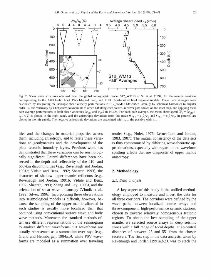
Ž .cific Ocean, and the Philippine Sea Fig. 1 . On thisscale, some of the major differences in path averagedshear velocities can be resolved by global tomo-graphic models. For example, model S12_WM13 of

Ž .Su et al. 1994 shows that Australia has higher shearvelocities than the oceanic paths in the upper 400 km

and that the central Pacific Ocean has a faster lidŽ .than the Philippine Sea Fig. 2 . These contrasts

reflect the lateral temperature andror compositionaldifferences in the upper mantle that we seek tounderstand. However, the picture of the upper mantleobtained from S12_WM13 and many other pub-lished global tomographic models is necessarily in-complete, because most were derived by holding theanisotropy and discontinuity structure constant dur-ing the inversion.

The purpose of our study is to investigate regionalvariations in the depths of upper mantle discontinu-

Ž . ŽFig. 1. Seismic corridors solid black lines modeled in this study; each corridor represents the average path connecting a source array open. Ž .circles, squares, and diamonds with a broad-band seismic station triangles . We model three corridors, one traversing Australia from NewŽ . Ž .Britain earthquakes to NWAO labeled AU3 , one traversing the central Pacific from TongarFiji events to HONrKIP labeled PA5 , and

Ž .one crossing the Philippine Sea basin from the Philippine events to MAJO labeled PHB3 . Ocean plate magnetic isochrons of Mueller et al.Ž . Ž1993 are plotted in white. Also plotted are arrows which represent the NUVEL-1 plate motions relative to a hotspot reference frame Gripp

.and Gordon, 1990 .

( )J.B. Gaherty et al.rPhysics of the Earth and Planetary Interiors 110 1999 21–41 23

Ž .Fig. 2. Shear wave structures obtained from the global tomographic model S12_WM13 of Su et al. 1994 for the seismic corridorsŽ . Ž . Ž .corresponding to the AU3 solid line , PA5 dashed line , and PHB3 dash-dotted line regional models. These path averages were

Žcalculated by integrating the isotropic shear velocity perturbations in S12_WM13 described laterally by spherical harmonics to angular.order 12, and vertically by Chebyshev polynomials to order 13 along each source–receiver path shown on the inset map, and applying these

Ž . Ž Žpath average perturbations to both shear velocities Õ and Õ in PREM. For each path average, the mean shear speed Õ s Õ qSH SV S SH. . ŽŽ . Ž . .Õ r2 is plotted in the right panel, and the anisotropic deviations from this mean Õ yÕ rÕ and Õ yÕ rÕ , in percent areSV SV S S SH S S

plotted in the left panels. The negative anisotropic deviations are associated with Õ , the positive with Õ .SV SH

ities and the changes in material properties acrossthem, including anisotropy, and to relate these varia-tions to geodynamics and the development of theplate–tectonic boundary layers. Previous work hasdemonstrated that these variations can be seismologi-cally significant. Lateral differences have been ob-served in the depth and reflectivity of the 410- and

Ž660-km discontinuities e.g., Revenaugh and Jordan,.1991a; Vidale and Benz, 1992; Shearer, 1993 , theŽcharacter of shallow upper mantle reflectors e.g.,

Revenaugh and Jordan, 1991b; Vidale and Benz,.1992; Shearer, 1993; Zhang and Lay, 1993 , and the

Žorientation of shear wave anisotropy Vinnik et al.,.1992; Silver, 1996 . Incorporating these observations

into seismological models is difficult, however, be-cause the sampling of the upper mantle afforded insuch studies is usually more localized than thatobtained using conventional surface wave and bodywave methods. Moreover, the standard methods of-ten use different representations of the seismogramto analyze different waveforms; SH waveforms are

Žusually represented as a summation over rays e.g.,.Grand and Helmberger, 1984a,b , while PSV wave-

forms are modeled as a summation over traveling

Žmodes e.g., Nolet, 1975; Lerner-Lam and Jordan,.1983, 1987 . The mutual consistency of the data sets

is thus compromised by differing wave-theoretic ap-proximations, especially with regard to the waveformsplitting effects that are diagnostic of upper mantleanisotropy.

2. Methodology

2.1. Data analysis

A key aspect of this study is the unified method-ology employed to measure and invert the data forall three corridors. The corridors were defined by thewave paths between localized source arrays andthree-component, high-performance seismic stations,chosen to traverse relatively homogeneous tectonicregions. To obtain the best sampling of the uppermantle, we selected source arrays in deep seismiczones with a full range of focal depths, at epicentraldistances of between 25 and 558 from the chosenreceivers. The first step in the data analysis, taken by

Ž .Revenaugh and Jordan 1991a,b,c , was to stack the

()

J.B.G

ahertyet

al.rP

hysicsof

theE

arthand

Planetary

Interiors110

199921

–41

24

Ž . Ž . Ž .Fig. 3. Summary of the frequency-dependent travel time data. Average phase delays dt for a the Australia corridor, b the Pacific corridor, and c the Philippine SeapŽ . Ž .corridor, referenced to corridor-specific isotropic starting models and plotted against frequency for surface waves top panels , SS and SSS waves middle , and S waves

Ž . Ž . Ž .bottom . Points with standard errors are averages of measurements for each seismic phase from vertical squares and transverse circles seismograms, summarizing thefrequency-dependent travel times used in the inversions; solid and dashed lines are corresponding averages computed for the models of Fig. 4. The total number of phase delaymeasurements summarized are: Australia, 797; Pacific, 1499; Philippine Sea, 1039.


ScS reverberations from a subset of these seismo-grams for the shear wave reflectivity profile of themantle within each seismic corridor. This procedurefirst involved fitting the waveforms of the primary

Ž .ScS and sScS phases zeroth-order reverberationsn n

to determine the whole-mantle ScS travel time andŽ .attenuation factor Q for each path. With thisScS

calibration, the travel times and amplitudes of theprimary reflections from upper mantle discontinuitiesŽ .first-order reverberations were determined via astacking and migration procedure. The resulting cor-ridor-specific profiles of mantle reflectivity providedthe vertical travel times to, and SV impedance con-trasts across, all mantle discontinuities. This proce-dure was able to detect, measure, and locateimpedance variations as small as 1%, and the verticaltravel times and impedance contrasts provide precise,layered frameworks for the regional upper mantlestructures. We follow the conventions of Revenaugh

Ž .and Jordan 1991b in designating internal disconti-Žnuities above 400 km by a capital letter Ms

Mohorovicic, H s Hales, G s Gutenberg, L s.Lehmann and TZ discontinuities by their nominal

depths in kilometers; e.g., 410, 520, 660, 710 and900.

The second step was to measure an extensive setof frequency-dependent travel times from surfacewaves, body waves, and guided waves of all polar-

Ž .izations Fig. 3 . The analyzed seismic phases in-cluded S, sS, SS, sSS, SSS, Sa, R , and G , and the1 1

travel times were measured by cross-correlating ob-served seismograms with spherical Earth synthetic

Žseismograms computed by mode summation Gee.and Jordan, 1992 . At the epicentral distances and

Ž .frequencies 10–45 mHz used here, these phases areaffected by complex interference of multiple refrac-tions, reflections, and conversions from upper mantlediscontinuities, and they show clear evidence ofsplitting between SH and P–SV components, indica-

Ž .tive of anisotropy Fig. 3 . Frechet kernels used to´invert these data accounted for radial anisotropy,frequency-dependent diffractions, and other wave-propagation effects, including the interference from

Žother seismic phases Gee and Jordan, 1992; Gaherty.et al., 1996 . The number of measured travel times

ranged from approximately 800 from the Australiancorridor to nearly 1500 from the Pacific corridor.Such data provide good constraints on the radially

Žanisotropic velocities and gradients especially the.shear velocities between the discontinuities.

2.2. InÕersion

The two data sets from each corridor were jointlyŽinverted for regional radially anisotropic trans-

.versely isotropic models of the upper mantle, de-Žfined by six medium parameters e.g., Dziewonski

. Ž .and Anderson, 1981 : mass density, r z ; the speedsof horizontally and vertically propagating P waves,

Ž . Ž .Õ z and Õ z ; the speed of horizontally propa-PH PVŽ .gating, transversely polarized shear waves, Õ z ;SH

the speed of a shear wave propagating either hori-zontally with a vertical polarization or vertically with

Ž .horizontal polarization e.g., ScS reverberations ,Ž .Õ z ; and a parameter that governs the variation ofSV

Ž .the wave speeds at oblique propagation angles, h z .The models are frequency dependent, with the atten-uation structure along each corridor chosen to satisfythe observed Q in conjunction with surface waveScS

amplitude data. Our modeling procedures soughtminimal structure: first-order discontinuities weresuppressed unless detected by ScS reverberations;linear gradients were maintained between discontinu-

Žities; second-order discontinuities i.e., changes ingradient between two observed first-order disconti-

.nuities were only allowed if a single layer wasŽunable to satisfy the data; and isotropy Õ sÕ ,PH PV

.Õ sÕ , hs1 was required wherever consistentSH SV

with the data. Various inversion experiments wereperformed to test for the depth distribution of theanisotropy. The non-linear analysis procedure wasfully iterated at least twice for each corridor, witheach iteration including complete remeasurement ofthe data using synthetic seismograms computed fromthe new model and recalculation of their associatedpartial derivatives.

The data sets were complementary, in that theScS reverberation data provided strong constraintson the discontinuity depths and SV impedance con-trasts, while the extensive shear wave travel timedata were most sensitive to the shear velocities be-tween discontinuities. Using the formal posterior un-certainties as a guide, we conservatively assess ourstandard errors of estimation to be of order 3–5 km

Žfor the depths of the major discontinuities M, G,.410, 660 , 5–10 km for the smaller discontinuities


Ž .H, L , approximately "0.05 kmrs in the layeraverages of Õ and Õ , and ;1% in shear anisot-SH SV

ropy through the upper mantle and TZ. Our shearwave data are relatively insensitive to the compres-sional velocities and density, however, and we con-strained these parameters by incorporating a comple-mentary set of mineral physics data. At six discretedepths between 250 and 780 km, we required the

Ž 2density r and bulk sound velocity Õ s Õ yf P2 .1r24Õ r3 to satisfy the estimates obtained by ItaS

Ž .and Stixrude 1992 for a pyrolite mineralogy, as-signing a standard error of "1% to each estimate.These parameters can be inferred with reasonableprecision from laboratory observations; moreover,the choice of a pyrolite composition is not particu-larly restrictive, since similar estimates for compet-

Žing mineralogical models e.g., high-aluminum pi-.clogite differ from pyrolite by less than the assignedŽ .errors Ita and Stixrude, 1992 . These constraints had

little effect on the estimated shear velocities, but theyensured that the relative behavior of the density,shear, and compressional profiles conform to realis-tic mineralogies.

We have completed the modeling for the threecorridors in Fig. 1, and the final models are pre-sented in Tables 1–3. A complete discussion of theanalysis and inversion is presented by Gaherty et al.Ž .1996 for the Pacific corridor, with details associ-ated with Australia and the Philippine Sea provided

Ž .by Gaherty and Jordan 1995 and Kato and JordanŽ .1998 , respectively. Here we investigate the re-gional variation of mantle layering as described bythese three models. Because the shear velocities arethe best resolved parameters in our model, they arethe focus of our discussion.

Fig. 4 displays the S wave structures from ourmodels, designated AU3, PA5, and PHB3 for theAustralia, Pacific, and Philippine Sea corridors, re-spectively. Comparing Figs. 2 and 4, it appears thatthe regional models capture a number of the impor-tant features of upper mantle structure that cannot bediscerned in S12_WM13. These features includesubstantial heterogeneity in lid and low-velocity zoneŽ .LVZ structure in the uppermost mantle, and largevariations in the discontinuity depths and amplitudes,in the maximum depth of the anisotropy, and in theshear-speed gradients, especially between 100 and400 km. Moreover, S12_WM13 has a large jump in

Ž .Õ across a Lehmann L discontinuity at 220 kmSŽ .inherited from its reference model, PREM , whilethe isotropic shear speeds at this depth are essentiallycontinuous in our models.

A simple visual evaluation indicates that our mod-els better characterize upper mantle structure in theseregions. Fig. 5 displays representative seismogramsfor the three corridors, and it compares these obser-vations with synthetics calculated for the path aver-aged models in Tables 1–3 as well as global model

Table 1Model AU3)

3Ž . Ž . Ž . Ž . Ž . Ž .z km r Mgrm Õ kmrs Õ kmrs Õ kmrs Õ kmrs h QSV SH PV PH m

0.0 2.85 3.62 3.62 6.05 6.05 1.00 30030.0 2.85 3.62 3.62 6.05 6.05 1.00 30030.0 3.30 4.28 4.40 8.00 8.15 0.90 30054.0 3.30 4.28 4.40 8.00 8.15 0.90 30054.0 3.40 4.56 4.68 8.23 8.52 0.90 300

252.0 3.44 4.52 4.70 8.28 8.61 0.90 300252.0 3.45 4.63 4.63 8.45 8.45 1.00 120406.0 3.58 4.80 4.80 8.88 8.88 1.00 120406.0 3.69 5.07 5.07 9.31 9.31 1.00 312499.0 3.85 5.19 5.19 9.64 9.64 1.00 312499.0 3.88 5.23 5.23 9.67 9.67 1.00 312659.0 4.00 5.58 5.58 10.21 10.21 1.00 312659.0 4.21 5.94 5.94 10.72 10.72 1.00 312861.0 4.50 6.28 6.28 11.21 11.21 1.00 312


Table 2Model PA5)


0.0 1.03 0.00 0.00 1.50 1.50 1.00 99995.0 1.03 0.00 0.00 1.50 1.50 1.00 99995.0 1.50 0.92 0.92 2.01 2.01 1.00 99995.2 1.50 0.92 0.92 2.01 2.01 1.00 99995.2 3.03 3.68 3.68 5.93 5.93 1.00 150

12.0 3.03 3.68 3.68 5.93 5.93 1.00 15012.0 3.34 4.65 4.84 8.04 8.27 0.90 15068.0 3.38 4.67 4.83 8.06 8.30 0.90 15068.0 3.35 4.37 4.56 7.88 8.05 0.90 50

166.0 3.41 4.26 4.34 8.04 8.09 1.00 50166.0 3.42 4.29 4.29 8.06 8.06 1.00 150415.0 3.58 4.84 4.84 8.92 8.93 1.00 150415.0 3.71 5.04 5.04 9.29 9.29 1.00 150507.0 3.85 5.20 5.20 9.64 9.64 1.00 150507.0 3.88 5.28 5.28 9.71 9.71 1.00 150651.0 4.02 5.43 5.43 10.11 10.11 1.00 150651.0 4.29 5.97 5.97 10.76 10.76 1.00 231791.0 4.46 6.23 6.23 11.08 11.08 1.00 231791.0 4.46 6.23 6.23 11.08 11.08 1.00 231801.0 4.46 6.24 6.24 11.10 11.10 1.00 231

Table 3Model PHB3a


0.0 1.03 0.00 0.00 1.50 1.50 1.00 99995.4 1.03 0.00 0.00 1.50 1.50 1.00 99995.4 1.50 0.92 0.92 2.10 2.10 1.00 99995.5 1.50 0.92 0.92 2.10 2.10 1.00 99995.5 2.83 3.48 3.48 6.27 6.27 1.00 140

16.9 2.83 3.48 3.48 6.27 6.27 1.00 14016.9 3.28 4.39 4.54 7.91 8.02 0.91 14051.0 3.28 4.39 4.54 7.91 8.02 0.91 14051.0 3.35 4.41 4.59 8.00 8.14 0.91 15089.3 3.35 4.41 4.59 8.00 8.14 0.91 14089.3 3.35 4.22 4.43 7.89 8.05 0.91 55

165.5 3.35 4.23 4.31 7.99 8.07 0.94 55165.5 3.35 4.27 4.27 8.03 8.03 1.00 140407.7 3.66 4.88 4.88 8.97 8.97 1.00 140407.7 3.76 5.12 5.12 9.36 9.36 1.00 140520.4 3.87 5.27 5.27 9.76 9.76 1.00 140520.4 3.88 5.34 5.34 9.77 9.77 1.00 140664.0 4.02 5.57 5.57 10.22 10.22 1.00 140664.0 4.35 5.78 5.78 10.66 10.66 1.00 231761.3 4.42 6.16 6.16 10.94 10.94 1.00 231761.3 4.44 6.19 6.19 11.02 11.02 1.00 231771.0 4.44 6.22 6.22 11.05 11.05 1.00 231

a Models are calculated at a reference frequency of 35 mHz and linearly interpolated between depths. Below the last depth listed, velocitiesŽ .and density are identical to PREM and Q remains constant. Q is set to the PREM value 57 823 throughout the mantle.m k


Ž Ž . .Fig. 4. Shear wave structures for the three regional models discussed in this study. The mean shear speeds Õ s Õ qÕ r2 for AU3S SH SVŽ . Ž . Ž .solid line , PA5 dashed line , and PHB3 dash-dotted line are plotted in the right panel, and the anisotropic deviations about these meansŽŽ . Ž . .Õ yÕ rÕ and Õ yÕ rÕ , in percent are plotted in the left panels. In all three models, Õ is the slower velocity, Õ is theSV S S SH S S SV SH

Ž .faster velocity. Depth intervals for the upper mantle discontinuities discussed in the text are shaded: the Gutenberg G discontinuityŽ .represents the lidrLVZ transition in the oceanic models, and the Lehmann L represents the termination of anisotropy, best observed in

Ž . Ž .AU3. The inset map keys the models to the appropriate seismic corridors, including the stations triangles and earthquakes dots used inthe data processing.

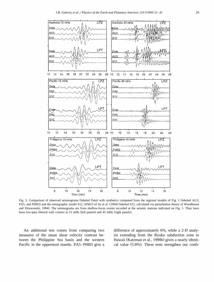
Ž .S12_WM13. At low frequencies left panels , bothour regional models and those derived by the globaltomography match the observations, but at higher

Ž .frequencies right panels , the latter show substantialdiscrepancies. The detailed seismic layering incorpo-rated in the regional models provides an improvedcapability for calculating the effects of wave propa-gation through the upper mantle.

2.3. Potential bias due to lateral heterogeneity

In constructing these models, we utilized a path-average approximation, which assumes that the ob-served waves effectively average heterogeneity be-tween source and receiver, and that the resulting 1-Dmodel represents the average velocity structure alongthe corridor. The choice of relatively homogenouspaths enhances the validity of this approximation,and we further improve the assumption by selec-tively downweighting observations with substantial

Žsampling outside the regions of interest the south-ernmost events in Tonga, or events internal to the

.Philippine archipelago, for example .

In the case of the Pacific model, we can test thisapproximation by examining a recent high-resolu-tion, 2-D image of shear velocities along the

Ž .Tonga–Hawaii corridor. Katzman et al. 1998ameasured an extensive set of travel time data from S,SS, SSS, R , G , and ScS-reverberation phases simi-1 1

Ž .lar to but more extensive than that used in theconstruction of PA5. These data were inverted using

Ž .2-D sensitivity kernels Zhao and Jordan, 1998 ,with PA5 as the reference model. The resultingmodel TH2 displays substantial along-path variabil-

Ž .ity in mean shear velocity "2.5% , shear waveŽ .anisotropy "1% , and depths to the 410- and 660-

Ž . Ž .km discontinuities "10 km Katzman et al., 1998a .This lateral heterogeneity does not compromisePA5’s representation of the average velocity alongthe corridor, however. Fig. 6 compares the meanshear speed in PA5 with the along-path average ofshear velocities in TH1. The two representations

Ž .differ negligibly -0.5% throughout the uppermantle and TZ, and similar conclusions can be drawnfrom comparisons of average discontinuity depth andanisotropy between the two models.


Ž . ŽFig. 5. Comparison of observed seismograms labeled Data with synthetics computed from the regional models of Fig. 1 labeled AU3,. Ž . ŽPA5, and PHB3 and the tomographic model S12_WM13 of Su et al. 1994 labeled S12, calculated via perturbation theory of Woodhouse

.and Dziewonski, 1984 . The seismograms are from shallow-focus events recorded at the seismic stations indicated on Fig. 1. They haveŽ . Ž .been low-pass filtered with corners at 15 mHz left panels and 45 mHz right panels .

An additional test comes from comparing twomeasures of the mean shear velocity contrast be-tween the Philippine Sea basin and the westernPacific in the uppermost mantle. PA5–PHB3 give a

difference of approximately 6%, while a 2-D analy-sis extending from the Ryuku subduction zone to

Ž .Hawaii Katzman et al., 1998b gives a nearly identi-Ž .cal value 5.8% . These tests strengthen our confi-


Fig. 6. Comparison of PA5 with the along-path average of the 2-DŽ .shear velocity model TH2 of Katzman et al. 1998a .

dence that the path average approximation providesmeaningful information for investigating mantle lay-ering in these and other regions.

2.4. Potential bias due to restricted anisotropic pa-rameterization

The apparent splitting between SH and P–SVŽ .observations Fig. 3 is direct evidence for seismic

anisotropy in the upper mantle. This anisotropy ismost likely related to the lattice-preferred orientationŽ .LPO of olivine in upper mantle peridotites causedby shearing during plate formation, translation, anddeformation, which induces 3-D directional asymme-

Žtry in the wave speeds e.g., Nicolas and Chris-.tensen, 1987 . A complete description of this anisot-

ropy requires 13 elastic parameters: the five parame-ters of radial anisotropy, which distinguish verticaland horizontal velocities; and eight additional param-eters which describe azimuthal velocity variationŽ .e.g., Montagner and Nataf, 1986 . The restriction of

Žour analyses to single-azimuth corridors which min-.imizes the impact of lateral heterogeneity limits us

to a radially anisotropic model. This limited parame-terization could potentially bias our results.

The magnitude of this bias depends in the lengthscale over which LPO is coherent, and we consider

two scenarios. The travel times used in our analysisrepresent integrals of a projection of the 3-D anisot-ropy onto the direction of wave propagation, with theSH times being dominated by the horizontal veloci-ties, and SV times dominated by vertical velocities.If the local anisotropy varies significantly along thepropagation path, then the azimuthal terms averageout, and radial anisotropy inferred from these traveltimes represents an unbiased path average of the

Žmedia e.g., Estey and Douglas, 1984; Jordan and.Gaherty, 1995 . This scenario seems to be appropri-

ate for the geologically complex continental litho-Ž .sphere in Australia Gaherty and Jordan, 1995 . Al-

ternatively, the local anisotropy may be coherentlyaligned over distances as large or larger than thecorridor lengths. Such a situation may occur inoceanic lithosphere, and in oceanic and continentalasthenosphere, where plate-scale anisotropy associ-ated with sea-floor spreading and present-day plate

Žmotion has been proposed e.g., Montagner, 1985;Nicolas and Christensen, 1987; Nishimura and

.Forsyth, 1989; Montagner and Tanimoto, 1991 . ForŽplausible values of local anisotropy 3–8%; Chris-

.tensen, 1984 , the projection of such large-scalehorizontal anisotropy onto the propagation path isexpected to yield radial anisotropy magnitudes that

Ž .are positive and large up to 5% for paths perpen-Ždicular or oblique to the LPO, but small and even

.negative for paths within "208 to this directionŽ .Kawasaki and Kon’no, 1984; Maupin, 1985 . Thevalues of the radial anisotropy parameters in ourmodels thus do not represent the true values of theseparameters in a complete azimuthal description. Weare primarily interested in the depth distribution ofanisotropy and its relationship to discontinuities andother structural features of the mantle, however, andin the oblique case, our models provide a robust

Ž .estimate of these attributes Maupin, 1985 . Thesubparallel case is problematic for even these generalinferences because at such angles a large-scale, co-herent anisotropic region could appear isotropicŽ .Leveque and Cara, 1983; Maupin, 1985 .´ ˆ

In our three models, we feel that this latter sce-nario is unlikely. Our corridors all are oblique or

Ž .perpendicular to current plate motion Fig. 1 , andthus should be sensitive to anisotropy due to thismechanism. The Philippine path does appear to benearly parallel to fossil spreading along its southern


half, but we do infer approximately 4% radial shearanisotropy in the lid in this model, and similar valuesare found on an east–west profile across the basinŽ .Katzman et al., 1998b . The Pacific path has a meanorientation of 50–608 relative to fossil spreading andalso has anisotropy of about 4%, consistent withexpected values for a sea-floor spreading mechanismŽ .Gaherty et al., 1996 . PA5 has proven to be a goodaverage model for subsequent analyses of lateralvariations in anisotropy across several Pacific corri-

Ž .dors Katzman et al., 1998a,b; Levin and Park, 1998 .Despite these consistencies, however, we retain thecaveat that ‘isotropic’ regions of our models could

Ž .be locally anisotropic, but with alignment that is acoherent and roughly parallel to the propagation

Ž .direction, or b incoherent over 3000–4000 km pathlengths.

3. Layering in the Earth’s mantle

The corridors in Fig. 1 traverse three distinct,tectonically homogeneous regions, and the corre-sponding models are representative of the seismicsignature of the associated tectonic regimes. TheAustralia corridor is predominantly characterized bycontinental crust, specifically a suite of Archeancratons and Proterozoic platforms that were assem-bled by 1400 Ma, with only minor subsequent inter-

Ž .nal reactivation e.g., Rutland, 1981 ; AU3 is thus amodel of a stable continent. The central Pacific pathis confined to 100–125 Ma oceanic crust, and PA5thus represents the upper mantle beneath an oldocean plate. The Philippine Sea corridor crosses thewestern part of the Philippine Sea plate, primarilythe Western Philippine Basin, the Shikoku basin, andthe intervening ridges and plateaus. The oceaniccrust in these regions appears to be largely of back-

Žarc origin, with an age range of 15–50 Ma Hall et.al., 1995 . PHB3 thus characterizes the upper mantle

beneath an oceanic plate that is significantly youngerthan, and has a distinct origin from, that associatedwith PA5.

We aim to understand the causative mechanismsof four distinctive features of the upper mantle mod-els by considering their regional variability. The firstthree correspond to depth intervals in the mean shear

Ž .velocity structure: 1 the velocities and discontinu-

ities associated with the lid and LVZ, between theŽ .Moho and approximately 200 km depth; 2 the

velocities and gradients between approximately 200Ž .km depth and the 410-km discontinuity; and 3 the

TZ, including the 410-, 520-, and 660-km disconti-nuities. The fourth is represented by the radiallyanisotropic zone and associated discontinuities, whichmay correspond to one or more of the above depthintervals.

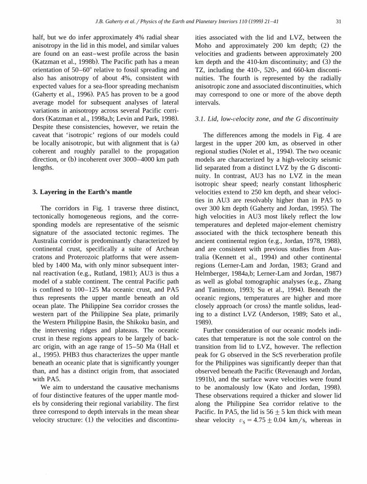
3.1. Lid, low-Õelocity zone, and the G discontinuity

The differences among the models in Fig. 4 arelargest in the upper 200 km, as observed in other

Ž .regional studies Nolet et al., 1994 . The two oceanicmodels are characterized by a high-velocity seismiclid separated from a distinct LVZ by the G disconti-nuity. In contrast, AU3 has no LVZ in the meanisotropic shear speed; nearly constant lithosphericvelocities extend to 250 km depth, and shear veloci-ties in AU3 are resolvably higher than in PA5 to

Ž .over 300 km depth Gaherty and Jordan, 1995 . Thehigh velocities in AU3 most likely reflect the lowtemperatures and depleted major-element chemistryassociated with the thick tectosphere beneath this

Ž .ancient continental region e.g., Jordan, 1978, 1988 ,and are consistent with previous studies from Aus-

Ž .tralia Kennett et al., 1994 and other continentalŽregions Lerner-Lam and Jordan, 1983; Grand and

.Helmberger, 1984a,b; Lerner-Lam and Jordan, 1987Žas well as global tomographic analyses e.g., Zhang

.and Tanimoto, 1993; Su et al., 1994 . Beneath theoceanic regions, temperatures are higher and more

Ž .closely approach or cross the mantle solidus, lead-Žing to a distinct LVZ Anderson, 1989; Sato et al.,

.1989 .Further consideration of our oceanic models indi-

cates that temperature is not the sole control on thetransition from lid to LVZ, however. The reflectionpeak for G observed in the ScS reverberation profilefor the Philippines was significantly deeper than that

Žobserved beneath the Pacific Revenaugh and Jordan,.1991b , and the surface wave velocities were found

Ž .to be anomalously low Kato and Jordan, 1998 .These observations required a thicker and slower lidalong the Philippine Sea corridor relative to thePacific. In PA5, the lid is 56"5 km thick with meanshear velocity Õ s4.75"0.04 kmrs, whereas inS


PHB3, it is 72"6 km thick with a mean velocityŽ .Õ s4.48"0.05 kmrs Fig. 4 . Since the area sam-S

pled in the Philippine Sea is younger than in thePacific, the increased depth to the G discontinuity isinconsistent with a thermally controlled transition

Žproposed in many previous studies e.g., Leeds et al.,.1974; Anderson and Regan, 1983 , which would

require a thinning lid with decreasing age. Thisinference is also supported by the magnitude of themean shear velocity difference; relative to the Pa-cific, velocities beneath the Philippine Sea are toolow to be explained by thermal differences aloneŽ .Kato and Jordan, 1998 .

The models are consistent with a scenario wherethe G in older oceanic regions is a compositionalboundary set by the depth of melting during the

Ž .production of the overlying oceanic crust Fig. 7 .The extraction of basaltic melt at a mid-ocean ridgegenerates two major compositional changes to themantle source region: it depletes it of Al, Ca, and Fe

Ž .relative to Mg e.g., Ringwood, 1975 , and it effi-Ž .ciently strips it of any volatiles H O, CO that are2 2

Ž .present Karato, 1986; Hirth and Kohlstedt, 1996 .The resulting compositional layering—dry, partially

Fig. 7. Schematic cross-section of oceanic upper mantle, depictingthe compositional layering hypothesized to give rise to the Gdiscontinuity. Decompression melting and extraction of basaltic

Ž .magma occurs in a narrow melt separation zone MSZ beneaththe ridge crest. Any volatiles present in the mantle source regionwill enter the melt phase, resulting in a dry layer of depleted

Ž .peridotite residuum overlying water-undersaturated ‘damp’ nor-mal mantle. This compositional boundary is preserved as the plateages. We argue that far from the partially molten near-ridgeenvironment, this contrast in volatile content is responsible for theobserved G discontinuity, and as such it represents the fossilizedbase of the MSZ. One prediction of this model is that the depth toG should be relatively constant for a given ocean basin far from

Ž .the ridge thick solid line . For comparison, if G corresponds to aŽ .critical isotherm thin line , then its depth should increase with

plate age.

depleted peridotite residuum underlain by ‘damp’Ž .hydrous but undersaturated fertile peridotite—per-sists as the plate translates away from the ridge. Themajor-element depletion increases the shear velocity

Žby less than 1% e.g., Fig. 8 in the work of JordanŽ ..1979 , but the volatile contrast could result in a

Ž .larger seismic discontinuity Karato, 1995 . By con-sidering the likely quantities and solubility ofvolatiles in oceanic upper mantle, Hirth and Kohlst-

Ž .edt 1996 estimated that the damp peridotite will betwo orders of magnitude less viscous than the overly-ing dry harzburgite owing to the water-enhanceddefect mobility in olivine. Because defect mobilityalso controls seismic Q, which in turn has an indirect

Ž .effect on seismic velocities, Karato 1995 suggestedthat the presence of water can reduce seismic veloci-ties by several percent. Building on these arguments,we hypothesize that G represents the seismic signa-ture of the relatively abrupt transition from drier tomore damp peridotite, and that it is coincident with a

Ž .sharp drop in Q Tables 2 and 3 and viscosityŽ .Hirth and Kohlstedt, 1996 . This hypothesis ex-plains several aspects of our regional velocity struc-

Ž .tures: the magnitude of the velocity drop 3–6% isconsistent with the mechanism predicted by KaratoŽ .1995 assuming the water content estimated by Hirth

Ž .and Kohlstedt 1996 ; the range of depth of thedry-to-wet transition predicted by Hirth and Kohlst-

Ž .edt 1996 is compatible with the depth of G in PA5and PHB3; and the abrupt transition from wet to drycan explain the sharpness of the seismic transitionŽconstrained by ScS reverberations to be less than

.30-km width . The scenario is similar to that recentlyŽ .proposed by Karato and Jung 1998 to explain the

seismic observations of Revenaugh and JordanŽ . Ž .1991b and Gaherty et al. 1996 .

The association of G with the depth of meltingsuggests that melting initiated deeper beneath thewestern part of Philippine Sea plate than beneath the

Ž .central Pacific 89 vs. 68 km depth, respectively .This implication is testable, because an increase indepth to melting should correspond to an increase incrustal thickness due to the larger volume of the meltcolumn. As shown in Fig. 8, the crust in PHB3Ž .11.5"1.5 km is significantly thicker than that in

Ž .PA5 6.8"1.0 km , in qualitative agreement withthis prediction. We evaluate the apparent correlation

Ž .between crustal thickness and depth to G melting


Fig. 8. Observed depth to the G discontinuity in PA5 and PHB3, plotted against the path averaged crustal thickness found in these models.Ž .Also plotted are curves for a simple polybaric, incremental batch, accumulative melting PIBAM model, after the work of Kinzler and

Ž .Grove 1993 . In this melting model, crustal thickness is a function of depth of initiation of melting, with average rate of melt generationbeing a free parameter. Our observed correlation between crustal thickness and depth to melt initiation corresponds to plausibleŽ .0.5–1.0%rkbar average melting rates.

quantitatively by comparing it with that predicted fora simple incremental, polybaric, near-fractional melt-

Ž .ing model Kinzler and Grove, 1993 . In this model,Ž .melting is initiated at a chosen depth pressure , and

Žit proceeds at a constant rate 0.5 and 1.0%rkbar of.ascent for the two curves in Fig. 8 , with 90% of the

melt being removed with each ascending step. Melt-ing terminates at 12 km depth, and the predictedcrustal thickness is a smooth function of the initial

Ž .depth of melting Fig. 8 . This model is a grosssimplification of melt generation in the near-ridgeenvironment; it ignores the likely functional depen-dence of melting rates and melt retention on pres-sure, temperature, and water content, for exampleŽe.g., McKenzie and Bickle, 1988; Plank and Lang-

.muir, 1992 . The discontinuity depths in our seismicmodels can be matched by such a model with anaverage melting rate of approximately 0.7%rkbar,however, and while we do not place any significancein this specific value, it implies that the associationof G with initial depth of melting is petrologicallyplausible.

An increase in the depth to melting beneath theŽancient Philippine Sea ridge environment relative to

.the ancient Pacific could be accomplished via one

of two mechanisms: a lowering of the melting tem-perature due to increased water content, or an in-crease in temperature. There is evidence for theformer; relatively high vesicularity and alkalinity ofbasaltic rocks drilled from the northwestern portion

Žof the Philippine Sea plate which our corridor tra-.verses are consistent with increased water content

and deeper melting within the ancient source regionŽ .Dick, 1982 . The long history of subduction sur-

Ž .rounding the Philippine Sea plate Hall et al., 1995provides a source of the extra water.

This hypothesis implies that there should be littleage-dependence in the depth to G within the stableŽ . Ž .non-ridge portion of an oceanic plate Fig. 7 . Thisprediction is in contrast with previous inferencesregarding the Pacific upper mantle, which indicate asteady increase of seismic lid thickness with increas-

Žing plate age due to thermal cooling Leeds et al.,1974; Anderson and Regan, 1983; Montagner and

.Jobert, 1983 . Such models result solely from theinversion of fundamental-mode surface wave data,which have poor resolution of lid thicknessŽ .Nishimura and Forsyth, 1989 . Direct observationsof reflections andror conversions from the G discon-

Žtinuity e.g., Revenaugh and Jordan, 1991b; Bock,


.1991 are required to unambiguously determine lidthickness, and we have utilized such observationshere.

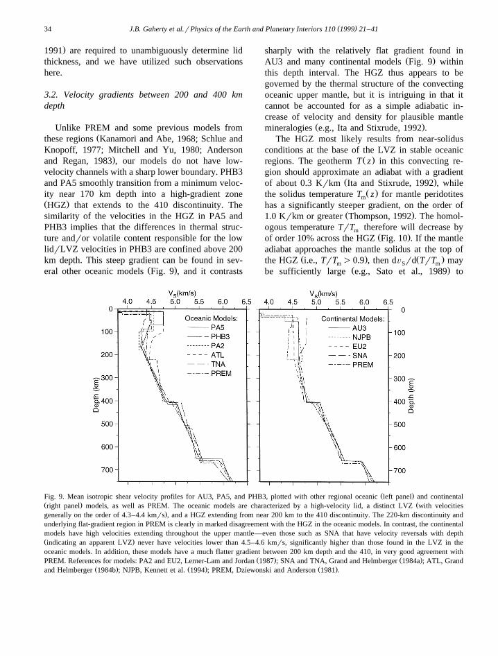
3.2. Velocity gradients between 200 and 400 kmdepth

Unlike PREM and some previous models fromŽthese regions Kanamori and Abe, 1968; Schlue and

Knopoff, 1977; Mitchell and Yu, 1980; Anderson.and Regan, 1983 , our models do not have low-

velocity channels with a sharp lower boundary. PHB3and PA5 smoothly transition from a minimum veloc-ity near 170 km depth into a high-gradient zoneŽ .HGZ that extends to the 410 discontinuity. Thesimilarity of the velocities in the HGZ in PA5 andPHB3 implies that the differences in thermal struc-ture andror volatile content responsible for the lowlidrLVZ velocities in PHB3 are confined above 200km depth. This steep gradient can be found in sev-

Ž .eral other oceanic models Fig. 9 , and it contrasts

sharply with the relatively flat gradient found inŽ .AU3 and many continental models Fig. 9 within

this depth interval. The HGZ thus appears to begoverned by the thermal structure of the convectingoceanic upper mantle, but it is intriguing in that itcannot be accounted for as a simple adiabatic in-crease of velocity and density for plausible mantle

Ž .mineralogies e.g., Ita and Stixrude, 1992 .The HGZ most likely results from near-solidus

conditions at the base of the LVZ in stable oceanicŽ .regions. The geotherm T z in this convecting re-

gion should approximate an adiabat with a gradientŽ .of about 0.3 Krkm Ita and Stixrude, 1992 , while

Ž .the solidus temperature T z for mantle peridotitesm

has a significantly steeper gradient, on the order ofŽ .1.0 Krkm or greater Thompson, 1992 . The homol-

ogous temperature TrT therefore will decrease bymŽ .of order 10% across the HGZ Fig. 10 . If the mantle

adiabat approaches the mantle solidus at the top ofŽ . Ž .the HGZ i.e., TrT )0.9 , then dÕ rd TrT maym S m

Ž .be sufficiently large e.g., Sato et al., 1989 to

Ž .Fig. 9. Mean isotropic shear velocity profiles for AU3, PA5, and PHB3, plotted with other regional oceanic left panel and continentalŽ . Žright panel models, as well as PREM. The oceanic models are characterized by a high-velocity lid, a distinct LVZ with velocities

.generally on the order of 4.3–4.4 kmrs , and a HGZ extending from near 200 km to the 410 discontinuity. The 220-km discontinuity andunderlying flat-gradient region in PREM is clearly in marked disagreement with the HGZ in the oceanic models. In contrast, the continentalmodels have high velocities extending throughout the upper mantle—even those such as SNA that have velocity reversals with depthŽ .indicating an apparent LVZ never have velocities lower than 4.5–4.6 kmrs, significantly higher than those found in the LVZ in theoceanic models. In addition, these models have a much flatter gradient between 200 km depth and the 410, in very good agreement with

Ž . Ž .PREM. References for models: PA2 and EU2, Lerner-Lam and Jordan 1987 ; SNA and TNA, Grand and Helmberger 1984a ; ATL, GrandŽ . Ž . Ž .and Helmberger 1984b ; NJPB, Kennett et al. 1994 ; PREM, Dziewonski and Anderson 1981 .


Fig. 10. Comparison of an estimated ‘damp’ solidus for pyrolitewith model geotherms for our three seismic corridors. Solidus isconstructed using the melting temperature T of pyrolite by Hirthm

Ž . 6and Kohlstedt 1996 with a water content of 815 Hr10 Si at180 km depth, and then extrapolating to greater depth assuming a

Ž .gradient of 1.0 Krkm bold line . Short-dashed lines representbounding water contents of "440 Hr106 Si, and long-dashed

Ž .lines are contours of constant homologous temperature TrT .m

The oceanic geotherms assume a cooling half-space with a poten-tial temperature of 14508C, merging into a mantle adiabat with a

Ž .gradient of 0.3 Krkm Ita and Stixrude, 1992 . The Australiageotherm is the 40 mWrm2 geotherm of Pollack and ChapmanŽ .1977 .

explain the high shear velocity gradient. This modelis consistent with the lower gradients beneath Aus-tralia; assuming the thickness of the thermal bound-ary layer is on the order of 300–400 km, the change

Žin TrT for a continental geotherm e.g., Pollackm.and Chapman, 1977 will be small over this depth

interval, and thus velocity will increase only slowlyŽ .Fig. 10 .

3.3. Transition zone

In the TZ, the Pacific model is slow, with a deepŽ .410-km discontinuity 415"3 km and a shallowŽ .660-km discontinuity 651"4 km . At the other

extreme, the Philippine Sea model has a fast TZ,Ž .with a shallow 410 408"3 km and deep 660

Ž .664"3 km . This relative behavior of discontinuitydepths and TZ velocities is in general agreementwith calculated Clapeyron slopes of phase changes inan olivine-dominated mantle; positive for the a–b

transition in olivine at 410, and negative for theŽ .g y Pv q Mw perovskite plus magnesiowustite

Ž .transition at 660 e.g., Bina, 1991 . All three modelswere constructed to provide good matches to thebulk sound velocity and density profiles of pyroliteŽ .Ita and Stixrude, 1992 throughout the TZ. Onaverage, the TZ beneath Australian corridor seems tobe slightly cooler than that beneath the Pacific corri-dor, in agreement with observed correlation between

Ž .thickened and therefore low-temperature TZ andŽ .old continents by Gossler and Kind 1996 . The

Philippine Sea TZ is even colder, consistent withŽprevious studies Masters et al., 1982; van der Hilst

et al., 1991; Fukao et al., 1992; Brudzinski et al.,.1997 . The low temperatures are perhaps due to the

presence of cooler material advected downward inthe surrounding subduction zones.

All three models contain small 520-km disconti-nuities, primarily to satisfy the ScS reverberation

Ždata. The 520 appears to be a global feature Shearer,.1990; Revenaugh and Jordan, 1991a most likely

Ž .caused by the broad 30-km width b–g transitionŽ . Ž .in Mg, Fe SiO Akaogi et al., 1989 , with a2 4

possible contribution from the exsolution of calciumŽ .perovskite Gasparik, 1990; Bina, 1991 . The veloc-

ity and density contrasts that we obtain for thisdiscontinuity are consistent with the available miner-

Ž .alogical data Bina, 1991; Rigden et al., 1991 . Dueto its small size relative to the 410 and 660, thedepth of the 520 is difficult to constrain from theScS reverberation profiles, and thus the depth varia-tion of this feature among the models is probably not

Žsignificant in all models, this depth has a standard.error of at least "10 km .

Fig. 4 displays very large differences in theshear-speed magnitude of the 660-km discontinuitybetween the three regions. Some of this differencemay be attributable to deficiencies in our models atthis depth. We restricted our parameterization to asingle layer below 660, and required the velocities atthe base of this layer to match those in PREM. Thiseffectively forces the layer to absorb any velocitydifferences sensed by the direct S waves, which turnbetween the 660 and approximately 1000 km depth.As a result, overly large differences in shear velocityand density may have been introduced between themodels in this depth interval. This is most apparentin the contrast between PHB3 and AU3, which have

Žnearly identical values of shear impedance product.of shear velocity and density across 660, but almost


a factor of two difference in velocity and densityŽ .jumps Fig. 4, Tables 1 and 3 .

Nevertheless, part of this difference is required bythe data. The shear impedance of 660-km in the threemodels is well-constrained by the ScS reverberationdata, and it varies systematically with depth of thereflector; the relatively deep 660 in PHB and AU3

Ž .are 30% smaller than the shallower by ;10 km660 in PA5. A similar trend was noted by Reve-

Ž .naugh and Jordan 1991a , who were unable to comeup with a satisfactory explanation. One possibility isthat it is due to the multi-component aspect of thediscontinuity. In a pyrolite mantle, two distinct, cou-pled phase transitions will occur near 660-km depth:the endothermic gyPvqMw transformation, which

Ž .occurs over an extremely narrow 1–5 km depthinterval; and the exothermic garnet–Pv transition,

Ž .which takes place over a wider 30–60 km depthŽrange Ita and Stixrude, 1992; Weidner and Wang,

.1998 . The combination of the two results in com-plex velocity and density increases, even for a sin-

Ž .gle-composition e.g., pyrolite mantle, and the formand sharpness of the transition is a strong function of

Ž .temperature Weidner and Wang, 1998 . Initial cal-culations indicate that the variability in 660 observedin our models can be explained by these coupledphase transitions in a pyrolite mantle. Such a modelhas the additional benefit of explaining why long-period data such as ScS reverberations indicate alarge 660 discontinuity, while higher frequency ob-

Žservations to which the garnet change would not.appear so discontinuous often require a smaller

Ž .discontinuity e.g., Walck, 1984 . A distributed gar-net transition also can explain the increased gradientsometimes observed just above andror below 660 in

Žsome models Walck, 1984; Brudzinski et al., 1997;.Estabrook and Kind, 1996; Vinnik et al., 1997 .

3.4. Anisotropic zone and the L discontinuity

Radial anisotropy is continuous throughout theuppermost mantle in all three regions. Its presence is

Ž .required by the differential travel times splittingŽ .between horizontally polarized SH and vertically

Ž .polarized SV shear waves. SH waves were alwaysobserved to be faster than SV waves, which requires

Ž .‘normal’ radial anisotropy Õ )Õ , Õ )Õ .SH SV PH PV

Anisotropy of this type is most plausibly related to

the LPO of olivine with fast axes aligned roughlyŽhorizontal e.g., Leveque and Cara, 1983; Jordan and´ ˆ

.Gaherty, 1995 . In the oceans, this alignment corre-sponds to the directions of past and present sea-floor

Žspreading e.g., Nicolas and Christensen, 1987;.Nishimura and Forsyth, 1989 , while in the conti-

nents, the upper mantle anisotropy appears to beinherited from episodes of horizontal shearing during

Žorogenic deformation Mainprice and Silver, 1993;.Silver, 1996 . In all three of our regions, the data

were satisfied by models with an average shearŽ . Žanisotropy ratio DÕ rÕ s 2 Õ y Õ r Õ qS S SH SV SH

.Õ of 3–4%, extending from the Moho to near 200SV

km depth.The depth extent of the anisotropy was con-

strained by the relative magnitude of observed split-Ž .ting in different wave types Fig. 3 . The largest

Žsplitting was observed in surface waves the Love–.Rayleigh discrepancy , requiring anisotropy in the

shallowest portions of the mantle, above 200 kmŽdepth Gaherty and Jordan, 1995; Gaherty et al.,

.1996 . Splitting was observed in SSS and SS wavesthat turn deeper in the upper mantle and TZ, but itwas smaller than that found in the surface waves,and it was unresolvable in S waves that turn in theTZ and lower mantle. This falloff in splitting stronglylimits the depth extent of the path average radialanisotropy. In particular, because SS and SSS phasesare sensitive to shallow anisotropy as well as anisot-ropy near their turning points deeper in the mantle,splitting in such phases can be explained by theradial anisotropy needed to satisfy the surface wave

Ž .splitting Fig. 11 , and any additional radial anisotro-py at larger depths must be smaller than 1%. Asnoted in Section 2.4, our radial models do not pre-clude azimuthal anisotropy at depths greater than

Ž250 km e.g., Montagner and Tanimoto, 1991; Tong.et al., 1994; Montagner and Kennett, 1996 , but such

anisotropy must either be aligned roughly parallel tothe propagation paths, or it must be variable in dip aswell as azimuth such as to integrate to isotropy overthe path length.

As an example of this depth sensitivity, our datafrom Australia are not consistent with models invok-ing a predominantly isotropic lithosphere underlainby a layer of anisotropy associated with plate mo-

Žtion-induced shear at its base i.e., between 200–400.km depth , as has been advocated beneath Australia


Ž .Fig. 11. Examples of clear, distinctive splitting of SS and SSS body waves by upper mantle anisotropy. a Splitting of a SS wave thatŽ . Ž .traversed the Australia corridor. b Splitting of a SSS wave that traversed the Pacific corridor. c Splitting of a SS wave that traversed the

Philippine Sea corridor. Left panels display examples of long-period seismograms centered on the SS or SSS arrival, band-passed between5–45 mHz. Each panel includes observed vertical- and transverse records, along with complete normal-mode synthetics for an isotropic

Ž .starting model, aligned on the LHZ SS or SSS arrival. In all three cases, the peak of the SS or SSS arrival on LHT is significantlyadvanced relative to the isotropic model, by 4–12 s. Right panels quantify the splitting in these waveforms. Symbols display the differences

Ž . Ž .between the tangential phase delays dt T and the vertical phase delays dt Z at each frequency, relative to the prediction of the isotropicp pŽ .starting models dashed lines . Solid lines represent the fit of models AU3, PA5, and PHB3 to these individual observations.

Ž .Leven et al., 1981; Tong et al., 1994 and elsewhereŽ .Vinnik et al., 1992, 1995 . Enforcing an isotropiccontinental lithosphere prevented us from fitting thesurface waves, and maintaining the fit to the SS andS splitting while introducing sufficient shallow ani-sotropy to satisfy the surface waves limited the

deeper average anisotropy to less than 1%. Addingeven 1% radial shear anisotropy to AU3 between250- and 400-km depth anisotropy would increasethe average SS splitting by approximately 3 s, whichdoes not match the observations. To be consistentwith this result, the LPO associated with plate mo-


tion-induced shear between 250–400 km must bevery weak, or it must be roughly parallel to thepropagation path, at a 30–408 angle to Australia’s

Žpredicted motion in a hotspot reference frame Fig..1 .

In AU3, radial anisotropy terminates rather sharplyacross the L discontinuity, and we have investigated

Žthis phenomenon in some detail Gaherty and Jordan,.1995 . The presence of high velocities throughout

the anisotropic layer in this model implies that theanisotropy is related to small-scale tectonic fabricgenerated in episodes of orogenic compression asso-

Žciated with tectospheric stabilization Silver and.Chan, 1991 , rather than active flow in the astheno-

Ž .sphere Karato, 1992 . Below L, such structureswere either annealed out subsequent to their forma-

Ž .tion Revenaugh and Jordan, 1991b , or were nevergenerated, perhaps because L coincides with a transi-

Žtion from dislocation to diffusion creep Karato,.1992 or because of an increase in the relative

amount of vertical deformation. The L discontinuityis located near the maximum depth of equilibrationobserved for suites of kimberlite xenoliths from sev-eral continental cratons, which averages approxi-

Ž .mately 220 km Finnerty and Boyd, 1987 . Thisequilibration level is interpreted to be the transitionfrom slow diapiric upwelling of kimberlite magmasŽ . Ž .or their precursors Green and Gueguen, 1974 tomuch more rapid upward transport by magma frac-

Žturing through a stronger lithosphere Spence and.Turcotte, 1990 . The L discontinuity may thus corre-

spond to the base of a mechanical boundary layerthat overlies a more mobile, dynamically active partof the continental tectosphere. The transition alsoappears to correspond to an abrupt downward in-crease in shear wave attenuation observed at about

Ž .this depth Table 1; Gudmundsson et al., 1994 .The termination of anisotropy in PA5 and PHB3

also occurs at L, but this boundary is poorly definedin these models because it is not large enough to beobserved in the reverberative profiles for these two

Ž .paths Revenaugh and Jordan, 1991b . The data didrequire a reduction of the radial anisotropy near thetransition from negative to positive velocity gradient

Žin the LVZ, however, and allowing a small -1%,.undetectable to ScS reverberations L discontinuity

accommodated this reduction with the minimal num-ber of model parameters. The drop in average anisot-

ropy in PA5 and PHB3 could correspond to thebottom of the zone of coherent horizontal shearŽ .either fossilized or active or to a change fromdislocation-dominated to diffusion-dominated creep

Ž .within the shear zone, as suggested by Karato 1992 .

4. Conclusions

We present a systematic analysis of the lateralvariability of mantle layering using three new re-gional seismic models. From this analysis we hy-

Ž .pothesize that: 1 the LVZ is predominantly anŽ .oceanic feature associated with high near-solidus

homologous temperatures in the shallow oceanic up-per mantle. The sharp transition from lid to LVZ ispredominantly determined by an increase in water

Ž .content in the LVZ. 2 Shear velocity gradientsbetween 200–400 km depth are significantly steeperbeneath oceans than continents, due to the rapid dropin homologous temperature across this depth interval

Ž .in oceanic environments. 3 Regional variability ofthe TZ velocities and discontinuities are consistent

Ž .with a pyrolite mantle. 4 When averaged overŽ .30–408 paths, strong seismic anisotropy )1% is

restricted to the upper 200–300 km of the uppermantle. In stable continents this anisotropy is rele-gated to the cold, mechanically stiff layer above theL discontinuity, while in oceans it extends throughthe lid into the LVZ.

These hypotheses regarding the mechanical, phase,and compositional layering of the mantle are notresolvable in the current generation of global models.Indeed, comparing Figs. 2 and 4 indicates that re-gional models such as these provide significant in-formation on lateral heterogeneity that is comple-mentary to that provided by tomographic models.

Our ability to fully test many of these hypothesesis restricted by the limitation of our 1-D modeling toregions of minimal tectonic complexity. For exam-ple, how exactly does the LVZ disappear in thetransition from a PA5-like structure to an AU3-likestructure across an ocean-continent boundary? Sucha question can only be answered with 2-D and 3-Dtomographic analyses that include lateral variability

Žof velocities, discontinuities, and anisotropy Katz-.man et al., 1998a,b . Building on AU3, PA5, and

PHB3 as reference models, such analyses should


greatly expand our understanding of seismic layeringin the near future.

Acknowledgements

We thank the Harvard and IRIS data centers fortheir assistance in collecting digital seismograms; R.Katzman for the TH2 path averages used in Fig. 7and helpful discussions; and T. Grove, G. Hirth, S.Karato, P. Puster, Y. Wang, and D. Weidner foruseful discussions. G. Ekstrom and J.-P. Montagnerprovided thorough reviews that led to substantialimprovement of the manuscript. Several figures were

Žgenerated using the free software GMT Wessel and.Smith, 1995 . This research was supported by the

Defense Special Weapons Agency under grantF49620-95-1-0051, and the National Science Foun-dation under grant EAR-94-18439.

References

Akaogi, M., Ito, E., Navrotsky, A., 1989. Olivine-modifiedspinel–spinel transitions in the system Mg SiO –Fe SiO :2 4 2 4

calorimetric measurements, thermochemical calculation, andgeophysical application. J. Geophys. Res. 94, 15671–15685.

Anderson, D.L., 1989. Theory of the Earth. Blackwell, Boston,MA.

Anderson, D.L., Regan, J., 1983. Upper mantle anisotropy and theoceanic lithosphere. Geophys. Res. Lett. 10, 841–844.

Bina, C.R., 1991. Mantle discontinuities: US Natl. Rep. Int. UnionGeodyn. Geophys. 1987–1990. Rev. Geophys. 29, 783–793.

Bock, G., 1991. Long-period S to P converted waves and theonset of partial melting beneath Oahu, Hawaii. Geophys. Res.Lett. 18, 869–872.

Brudzinski, M.R., Chen, W.-P., Nowack, R.L., Huang, B.-S.,1997. Variations of P wave speeds in the mantle transitionzone beneath the northern Philippine Sea with implications onmantle dynamics. J. Geophys. Res. 102, 11815–11827.

Christensen, N.I., 1984. The magnitude, symmetry, and origin ofupper mantle anisotropy based on fabric analyses of ultramafictectonites. Geophys. J. R. Astron. Soc. 76, 89–111.

Dick, H.J.B., 1982. The petrology of two back-arc basins in thenorthern Philippine Sea. Am. J. Sci. 282, 644–700.

Dziewonski, A.M., Anderson, D.L., 1981. Preliminary referenceEarth model. Phys. Earth Planet. Int. 25, 297–356.

Estabrook, C.H., Kind, R., 1996. The nature of the 660-km uppermantle seismic discontinuity from precursors to the PP phase.Science 274, 1179–1182.

Estey, L.H., Douglas, B.J., 1984. Upper mantle anisotropy: apreliminary model. J. Geophys. Res. 91, 11393–11406.

Finnerty, A.A., Boyd, F.R., 1987. Thermobarometry for garnetperidotites: basis for the determination of thermal and compo-

Ž .sitional structure of the upper mantle. In: Nixon, P.H. Ed. ,Mantle Xenoliths. Wiley-Interscience, Chichester, pp. 381–402.

Fukao, Y., Obayashi, M., Inoue, H., Nenbai, M., 1992. Subduct-ing slabs in the mantle transition zone. J. Geophys. Res. 97,4809–4822.

Gaherty, J.B., Jordan, T.H., 1995. Lehmann discontinuity as thebase of an anisotropic layer beneath continents. Science 268,1468–1471.

Gaherty, J.B., Jordan, T.H., Gee, L.S., 1996. Seismic structure ofthe upper mantle in a central Pacific corridor. J. Geophys. Res.101, 22291–22309.

Gasparik, T., 1990. Phase relations in the transition zone. J.Geophys. Res. 95, 15751–15769.

Gee, L.S., Jordan, T.H., 1992. Generalized seismological datafunctionals. Geophys. J. Int. 111, 363–390.

Gossler, J., Kind, R., 1996. Seismic evidence for very deep rootsof continents. Earth Planet. Sci. Lett. 138, 1–13.

Grand, S.P., Helmberger, D.V., 1984a. Upper mantle shear struc-ture of North America. Geophys. J. R. Astron. Soc. 76,399–438.

Grand, S.P., Helmberger, D.V., 1984b. Upper mantle shear struc-ture beneath the northwest Atlantic Ocean. J. Geophys. Res.89, 11465–11475.

Green, H.W., Gueguen, Y., 1974. Origin of kimberlite pipes bydiapiric upwelling in the upper mantle. Nature 249, 617–620.

Gripp, A.E., Gordon, R.G., 1990. Current plate velocities relativeto the hotspots incorporating the NUVEL-1 global plate mo-tion model. Geophys. Res. Lett. 17, 1109–1112.

Gudmundsson, O., Kennett, B.L.N., Goody, A., 1994. Broad-bandobservations of upper mantle seismic phases in northern Aus-tralia and the attenuation structure in the upper mantle. Phys.Earth Planet. Int. 84, 207–226.

Hall, R., Fuller, M., Ali, J., Anderson, C.D., 1995. The PhilippineSea plate: magnetism and reconstructions. In: Taylor, B.,

Ž .Natland, J. Eds. , Active Margins and Marginal Basins of theWestern Pacific. Geophysical Monograph 68. American Geo-physical Union, Washington, DC, pp. 371–404.

Hirth, G., Kohlstedt, D.L., 1996. Water in the oceanic uppermantle: implications for rheology, melt extraction, and theevolution of the lithosphere. Earth Planet. Sci. Lett. 144,93–108.

Ita, J., Stixrude, L., 1992. Petrology, elasticity, and composition ofthe mantle transition zone. J. Geophys. Res. 97, 6849–6866.

Jordan, T.H., 1978. Composition and development of the conti-nental tectosphere. Nature 274, 544–548.

Jordan, T.H., 1979. Mineralogies, densities, and seismic velocitiesof garnet lherzolites and their geophysical implications. In:

Ž .Boyd, F.R., Meyer, H.O.A. Eds. , The Mantle Sample: Inclu-sions in Kimberlites and Other Volcanics. American Geophys-ical Union, Washington, DC, pp. 1–14.

Jordan, T.H., 1988. Structure and formation of the continentaltectosphere. J. Petrol. Special Lithosphere Issue, 11–37.

Jordan, T.H., Gaherty, J.B., 1995. Stochastic modeling of small-scale, anisotropic structures in the continental upper mantle.


Proceedings of the 17th Annual Seismic Research Symposium,PL-TR-95-2108. Phillips Laboratory, MA, pp. 433–451.

Kanamori, H., Abe, K., 1968. Deep structure of island arcs asrevealed by the surface waves. Bull. Earthquake Res. Inst.Univ. Tokyo 86, 1001–1025.

Karato, S.-I., 1986. Does partial melting reduce the creep strengthof the upper mantle. Nature 319, 309–310.

Karato, S.-I., 1992. On the Lehmann discontinuity. Geophys. Res.Lett. 19, 2255–2258.

Karato, S.-I., 1995. Effects of water on seismic wave velocities inthe upper mantle. Proc. Jpn. Acad., Ser. B 71, 61–66.

Karato, S.-I., Jung, H., 1998. Water, partial melting and the originof the seismic low-velocity and high attenuation zone in theupper mantle. Earth Planet. Sci. Lett. 157, 193–207.

Kato, M., Jordan, T.H., 1998. Seismic structure of the uppermantle beneath the western Philippine Sea. Phys. Earth Planet.Int., in press.

Katzman, R., Zhao, L., Jordan, T.H., 1998a. High-resolution, 2-Dvertical tomography of the central-Pacific mantle using ScSreverberations and frequency-dependent travel times. J. Geo-phys. Res. 103, 17933–17971.

Katzman, R., Zhao, L., Jordan, T.H., 1998b. Seismic structure ofthe mantle between Ryukyu and Hawaii: implications for theHawaiian swell. J. Geophys. Res., submitted.

Kawasaki, I., Kon’no, F., 1984. Azimuthal anisotropy of surfacewaves and the possible type of the seismic anisotropy due topreferred orientation of olivine in the uppermost mantle be-neath the Pacific Ocean. J. Phys. Earth 32, 229–244.

Kennett, B.L.N., Gudmundsson, O., Tong, C., 1994. The uppermantle S and P velocity structure beneath northern Australiafrom broad-band observations. Phys. Earth Planet. Int. 86,85–98.

Kinzler, R.J., Grove, T.L., 1993. Corrections and further discus-sion of the primary magmas of mid-ocean ridge basalts, 1 and2. J. Geophys. Res. 98, 22339–22347.

Leeds, A.R., Knopoff, L., Kausel, E.G., 1974. Variations in uppermantle structure under the Pacific Ocean. Science 186, 141–143.

Lerner-Lam, A.L., Jordan, T.H., 1983. Earth structure from funda-mental and higher-mode waveform analysis. Geophys. J. R.Astron. Soc. 75, 759–797.

Lerner-Lam, A.L., Jordan, T.H., 1987. How thick are the conti-nents?. J. Geophys. Res. 92, 14007–14026.

Leven, J.H., Jackson, I., Ringwood, A.E., 1981. Upper mantleseismic anisotropy and lithospheric decoupling. Nature 289,234–239.

Leveque, J.J., Cara, M., 1983. Long-period Love wave overtone´ ˆdata in North America and the Pacific Ocean: new evidencefor upper mantle anisotropy. Phys. Earth Planet. Int. 33,164–179.

Levin, V., Park, J., 1998. Quasi-Love phases between Tonga andHawaii: observations, simulations, and explanations. J. Geo-phys. Res., in press.

Mainprice, D., Silver, P.G., 1993. Interpretation of SKS wavesusing samples from the subcontinental lithosphere. Phys. EarthPlanet. Int. 78, 257–280.

Masters, G., Jordan, T.H., Silver, P.G., Gilbert, J.F., 1982. As-

pherical Earth structure from fundamental spheroidal-modedata. Nature 298, 609–613.

Maupin, V., 1985. Partial derivatives of surface wave phasevelocities for flat anisotropic models. Geophys. J. R. Astron.Soc. 83, 379–398.

McKenzie, D., Bickle, M.J., 1988. The volume and compositionof melt generated by extension of the lithosphere. J. Petrol. 29,625–679.

Mitchell, B.J., Yu, G., 1980. Surface wave dispersion, regional-ized velocity models, and anisotropy of the Pacific crust andupper mantle. Geophys. J. R. Astron. Soc. 63, 497–514.

Montagner, J.-P., 1985. Seismic anisotropy of the Pacific Oceaninferred from long-period surface waves dispersion. Phys.Earth Planet. Int. 38, 28–50.

Montagner, J.-P., Jobert, N., 1983. Variation with age of the deepstructure of the Pacific Ocean inferred from very long-periodRayleigh wave dispersion. Geophys. Res. Lett. 10, 273–276.

Montagner, J.-P., Kennett, B.L.N., 1996. How to reconcile bodywave and normal-mode reference Earth models. Geophys. J.Int. 125, 229–248.

Montagner, J.-P., Nataf, H.C., 1986. A simple method for invert-ing the azimuthal anisotropy of surface waves. J. Geophys.Res. 91, 511–520.

Montagner, J.-P., Tanimoto, T., 1991. Global upper mantle to-mography of seismic velocities and anisotropy. J. Geophys.Res. 96, 20337–20351.

Mueller, R.D., Roest, W.R., Royer, J.-Y., Gahagan, L.M., Sclater,J.G., 1993. A digital age map of the ocean floor. SIO Refer-ence Series 93–30. Scripps Institute of Oceanography, LaJolla, CA.

Nicolas, A. Christensen, N.I., 1987. Formation of anisotropy inupper mantle peridotites: a review. In: Fuchs, K., Froidevaux,

Ž .C. Eds. , Composition, Structure, and Dynamics of Litho-sphere–Asthenosphere System. Geodyn. Ser., Vol. 16. Ameri-can Geophysical Union, Washington, DC, pp. 111–123.

Nishimura, C.E., Forsyth, D.W., 1989. The anisotropic structureof the upper mantle in the Pacific. Geophys. J. 96, 203–229.

Nolet, G., 1975. Higher Rayleigh modes in western Europe.Geophys. Res. Lett. 2, 60–62.

Nolet, G., Grand, S.P., Kennett, B.L.N., 1994. Seismic hetero-geneity in the upper mantle. J. Geophys. Res. 99, 23753–23766.

Plank, T., Langmuir, C.H., 1992. Effects of the melting regime onthe composition of the oceanic crust. J. Geophys. Res. 97,19749–19770.

Pollack, H.N., Chapman, D.S., 1977. On the regional variation ofheat loss, geotherms, and lithospheric thickness. Tectono-physics 38, 279–296.

Revenaugh, J.S., Jordan, T.H., 1991a. Mantle layering from ScSreverberations: 1. Waveform inversion of zeroth-order rever-berations. J. Geophys. Res. 96, 19749–19762.

Revenaugh, J.S., Jordan, T.H., 1991b. Mantle layering from ScSreverberations: 2. The transition zone. J. Geophys. Res. 96,19763–19780.

Revenaugh, J.S., Jordan, T.H., 1991c. Mantle layering from ScSreverberations: 3. The upper mantle. J. Geophys. Res. 96,19781–19810.


Rigden, S.M., Gwanmesia, G.D., Fitzgerald, J.D., Jackson, I.,Lieberman, R.C., 1991. Spinel elasticity and the seismic struc-ture of the transition zone of the mantle. Nature 345, 143–145.

Ringwood, A.E., 1975. Composition and Petrology of the Earth’sMantle. McGraw-Hill, New York.

Rutland, R.W.R., 1981. Structural framework of the AustralianŽ .Precambrian. In: Hunter, D.R. Ed. , Precambrian of the

Southern Hemisphere. Elsevier, Amsterdam, pp. 1–32.Sato, H., Sacks, I.S., Murase, T., 1989. The use of laboratory

velocity data for estimating temperature and partial melt frac-tion in the low-velocity zone: comparison with heat flow andelectrical conductivity studies. J. Geophys. Res. 94, 5689–5704.

Schlue, J.W., Knopoff, L., 1977. Shear wave polarization anisot-ropy in the Pacific basin. Geophys. J. R. Astron. Soc. 49,145–165.

Shearer, P.M., 1990. Seismic imaging of upper mantle structurewith new evidence for a 520-km discontinuity. Nature 344,121–126.

Shearer, P.M., 1993. Global mapping of upper mantle reflectorsfrom long-period SS precursors. Geophys. J. Int. 115, 878–904.

Silver, P.G., 1996. Seismic anisotropy beneath the continents:probing the depths of geology. Annu. Rev. Earth Planet. Sci.24, 385–432.

Silver, P.G., Chan, W.W., 1991. Shear wave splitting and subcon-tinental mantle deformation. J. Geophys. Res. 96, 16429–16454.

Spence, D.A., Turcotte, D.L., 1990. Buoyancy-driven magmafracture: a mechanism for ascent through the lithosphere andthe emplacement of diamonds. J. Geophys. Res. 95, 5133–5139.

Su, W.-J., Woodward, R.L., Dziewonski, A.M., 1994. Degree 12model of shear velocity heterogeneity in the mantle. J. Geo-phys. Res. 99, 6945–6980.

Thompson, A.B., 1992. Water in the Earth’s upper mantle. Nature358, 295–302.

Tong, C., Gudmundsson, O., Kennett, B.L.N., 1994. Shear wavessplitting in refracted waves returned from the upper mantle

transition zone beneath northern Australia. J. Geophys. Res.99, 15783–15799.

van der Hilst, R.D., Engdahl, R., Spakman, W., Nolet, G., 1991.Tomographic imaging of subducted lithosphere below north-west Pacific island arcs. Nature 353, 37–43.

Vidale, J.E., Benz, H.M., 1992. Upper mantle seismic discontinu-ities and the thermal structure of subduction zones. Nature356, 678–683.

Vinnik, L.P., Makeyeva, L.I., Milev, A., Usenko, A.Y., 1992.Global patterns of azimuthal anisotropy and deformations inthe continental mantle. Geophys. J. Int. 111, 433–447.

Vinnik, L.P., Green, R.W.E., Nicolaysen, L.O., 1995. Recentdeformations of the deep continental root beneath southernAfrica. Nature 375, 50–52.

Vinnik, L.P., Chevrot, S., Montagner, J.-P., 1997. Evidence for astagnant plume in the transition zone?. Geophys. Res. Lett. 24,1007–1010.

Walck, M., 1984. The P wave upper mantle structure beneath anactive spreading center: the Gulf of California. Geophys. J. R.Astron. Soc. 76, 697–723.

Weidner, D.J., Wang, Y., 1998. Chemical and clapyron inducedbuoyancy at the 660-km discontinuity. J. Geophys. Res. 103,7431–7442.

Wessel, P., Smith, W.H.F., 1995. New version of generic mappingtools released. Eos 76, 329.

Woodhouse, J.H., Dziewonski, A.M., 1984. Mapping the uppermantle: three-dimensional modeling of Earth structure by in-version of seismic waveforms. J. Geophys. Res. 89, 5953–5986.

Zhang, Z., Lay, T., 1993. Investigation of upper mantle disconti-nuities near northwestern Pacific subduction zones using pre-cursors to sSH. J. Geophys. Res. 98, 4389–4406.

Zhang, Y.-S., Tanimoto, T., 1993. High-resolution global uppermantle structure and plate tectonics. J. Geophys. Res. 98,9793–9823.

Zhao, L., Jordan, T.H., 1998. Sensitivity of frequency-dependenttravel times to laterally heterogeneous, anisotropic Earth struc-ture. Geophys. J. Int. 133, 683–704.

seismological structure of the upper mantle: a regional...

Documents