seismic performance evaluation of different …

SEISMIC PERFORMANCE EVALUATION OF DIFFERENT

RETROFITTING SCHEMES USING PUSHOVER ANALYSIS.

SK. MD. GOLAM RABBI

MASTER OF SCIENCE IN CIVIL ENGINEERING (STRUCTURAL)

DEPARTMENT OF CIVIL ENGINEERING

BANGLADESH UNIVERSITY OF ENGINEERING AND TECHNOLOGY

DHAKA-1000, BANGLADESH

MAY, 2019



by

SK. MD. GOLAM RABBI

A thesis submitted to the Department of Civil Engineering of Bangladesh University of

Engineering and Technology,Dhaka in partial fulfillment of the requirements for

the degree of

MASTER OF SCIENCE IN CIVIL ENGINEERING (STRUCTURAL)

DEPARTMENT OF CIVIL ENGINEERING

BANGLADESH UNIVERSITY OF ENGINEERING AND TECHNOLOGY

DHAKA-1000, BANGLADESH

MAY, 2019

iv

ACKNOWLEDGEMENT

Thanks to Almighty Allah for HIS Gracious, unlimited Kindness and with the

Blessings of whom the good deeds are fulfilled.

The author wishes to express his deepest gratitude to Dr. RupakMutsuddy,Assistant

professor,Department of Civil Engineering,BUET, Dhaka for his continuous guidance,

invaluable suggestions and affectionate encouragement at every stage of this study.

The author wishes to express his profound gratitude to Engr. Khandakar Md. Wahid

Sadique, Executive Engineer,North Dhaka (RAJUK) Division&Urban Resilience

Project (RAJUK), for his continuous support and allowing the use of different facilities

in connection with RAJUK to complete the thesis work.

A very special debt of deep gratitude is offered to the author’s parents, wife,and brother

for their continuous encouragement and cooperation during this study.

v

ABSTRACT

The traditional approach to seismic design is a force-based design where there is no measure of the deformation capability of a member or of a building. According to Bangladesh national building code,2006the buildings are designed with equivalent static force method, response spectrum method and time history analysis. However, the actual performance of a structure can hardly be found by these methods. Structural failures in recent earthquake have exposed the weakness of current design procedures and leads to the development of Performance Based Earthquake Engineering (PBEE).

As a relatively new development, Pushover-based seismic evaluation and design methods offered a great opportunity to engineers. Applied Technology Council (ATC-40),1996 and Federal Emergency Management Agency-(FEMA),2000proposed a simplified nonlinear static analysis (Pushover Analysis) procedure for PBEE which provides a better understanding about the actual behavior of the structures during earthquake. There are established numerical tools like ETABS v 9.7.4 developed by Computers and Structures Inc..1995which can perform the pushover analysis.

The present study investigates and compares the seismic performance of two existing buildings as per as built structural drawings by pushover analysis. Among the two buildings one is airregular shaped government office buildingand another one is a regular shapedgovernment residential building which are located at different locationsof Dhaka city.The buildings are of6 storied and constructed 20 years ago. Different infill conditions (i.e. bare frame, full infilled and soft ground storey)along with different earthquake conditions(i.e. serviceability earthquake, design basis earthquake and maximum earthquake) were considered during analysis. For different conditions mainly a structure is analyzed with the help of capacity curve, capacity spectrum,deflection,drift and seismic performance level. Effect of infill is modelled using equivalent strut width theory.

It is found that performance of full infilled frame condition is better than that of bare frame condition. Capacity curve of the both structures meets the demand curve at lower displacement value. Lateral drift ratios are less than that of bare frame structure. Investigation of building with soft storey condition shows that it contains seismic deficiencies and need some remedial measures or retrofitting.

The performances of the structures with different remedialmeasures (i.e. insertion of shear wall,buttresswall,column jacketing) have been studied both individually and combindly. Among the considered retrofitting measures "insertion of shear wall" shows better performance over "column jacketing and buttress wall" in terms of lateral inelastic drift ratio and number of hinges formed.

vi



TABLE OF CONTENTS

Page No

Certificate of approval ii

Declaration iii

Acknowledgement iv

Abstract v

Table of Contents vi

List of Tables xiii

List of Figures xvii

List of Symbols xxiv

Chapter 1 Introduction

1.1 General 1

1.2 Back Ground And Present State of the Problem 2

1.3 Objective and Scope of the Study 3

1.4 Outline of the Methodology 4

1.5 Layout of the Thesis 5

Chapter 2 Literature Review

2.1 Introduction 6

2.2 Earthquake Ground Motion 6

2.3 Ground Motion And Building Frequencies 7

2.4 Response Spectra 8

2.5 Analysis of Structure Due To Earthquake Forces 9

2.5.1 Equation of Motion: Earthquake Excitation 9

2.5.2 Code Specified Equivalent Static Load Method 10

2.5.3 Response Spectrum Analysis 11

2.6 Earthquake Loading In The Light of BNBC 14

2.6.1 Equivalent Static Load Method 14

2.6.2 Calculation of Base Shear 14

2.6.3 Zone Coefficient, Z 15

2.6.4 Structure Importance Coefficient, I 15

vii

Page No

2.6.5 Seismic Dead Load, W 15

2.6.6 Response Modification Factor, R 15

2.6.7 Numeric Coefficient, C 16

2.7 Response Spectrum Method 17

2.8 Time History Analysis 18

2.9 Limitation of BNBC 2006 18

2.9.1 The Zoning Map 18

2.9.2 Structure Period 18

2.9.3 Base Shear Distribution 18

2.10 Seismic Strengthening 19

2.11 Retrofit Strategies 19

2.11.1 Technical Strategis 20

2.11.2 Management Strategies 27

2.12 Past Research on Seismic Performance Evaluation

of different Retrofitting Schemes Using Non-Linear Analysis 28

Chapter 3 Concept of Performance Based Design

3.1 General 33

3.2 Seismic Analysis Methods 33

3.3 Methods to Perform Simplified Non Linear Analysis 34

3.3.1 Capacity Curve of a Structure 35

3.3.2 Demand Curve of a Structure 35

3.3.3 Performance Point of a Structure 36

3.4 Non Linear Static (Push Over) Analysis 36

3.4.1 Capacity Spectrum Method 39

3.4.2 Displacement Coefficient Method 39

3.5 Seismic Performance Evaluation 39

3.6 Nonlinear Static Procedure for Capacity Evaluation of Structures 40

3.7 Structural Performance Levels and Ranges 41

3.7.1 Immediate occupancy structural performance level (S-1) 42

3.7.2 Damage control structural performance range (S-2) 43

3.7.3 Life safety structural performance level (S-3) 43

viii

Page No

3.7.4 Limited safety structural performance range (S-4) 44

3.7.5 Collapse prevention structural performance level (S-5) 44

3.8 Target Building Performance Levels 44

3.9 Response Limits 45

3.9.1 Global building acceptability limits 45

3.9.1.1 Gravity Load 45

3.9.1.2 Lateral Load 45

3.9.2 Element and component acceptability limits 46

3.9.2.1 Primary and secondary elements and components 46

3.9.2.2 Deformation of force controlled action 46

3.9.2.3 Deformation Controlled and Force Controlled

Behaviour 46

3.10 Acceptability Limit 48

3.11 Seismic Demand 49

3.11.1 The Serviceability Earthquake(SE) 50

3.11.2 The design earthquake (DE) 50

3.11.3 The maximum earthquake (ME) 50

3.12 Development of Elastic Site Response Spectra 50

3.12.1 Seismic Zone 51

3.12.2 Seismic Source Type 51

3.12.3 Near Source Factor 51

3.12.4 Seismic Coefficients 51

3.13 Element Hinge Property 51

3.13.1 Concrete Axial Hinge 52

3.13.2 Concrete moment hinge and concrete P-M-M hinge 52

3.13.3 Concrete Shear Hinge 53

3.14 Concrete Frame Acceptability Limits 54

3.15 Hinge Properties for Modeling 54

3.16 Assumption for Pushover Analysis 55

Chapter 4 Effect of Masonry Infill in RC Buildings

4.1 Introduction 56

4.2 Computational Modeling of Infill Panel 59

ix

Page No

4.2.1 Equivalent strut method 59

4.2.2 Equivalent strut width 60

4.2.3 Eccentricity of equivalent strut 62

4.3 Perforated Panels 63

4.4 Partially Infilled Frames 64

4.5 Existing Infill Damage 64

4.6 Properties to be Determined 65

4.7 Calculation of Equivalent Strut Width 65

Chapter 5 Seismic Performance Evaluation of Two 06 (Six) Storey

RC Buildings

5.1 General 66

5.2 Structural Characteristic Features of Building 1 66

5.3 Performance Evaluation of The Building 1 67

5.4 Calculation and Selection of Seismic Coefficient For Building 1 74

5.5 Performance Evaluation of Bare Frame Condition of Building 1 69

5.5.1 Hinge formation Status of Bare Condition of Building 1 72

5.5.2 Lateral Drift Ratio for Bare Frame Condition of Building 1 73

5.6 Performance Evaluation of Full Infilled Condition of Building 1 74

5.6.1 Hinge formation Status of Full Infilled Condition of

Building1 77

5.6.2 Lateral Drift Ratio for Full Infilled Condition of Building 1 78

5.7 Performance Evaluation of Soft Storey Condition of Building 1 79

5.7.1 Hinge formation Status for Soft Storey Condition of

Building 1 82

5.7.2 Lateral Drift Ratio for Soft Storey Condition Of Building 1 82

5.8 Comparison of The Performance Evaluation of The Building 1

Considered for Analysis 83

5.8.1 Comparison Of Hinge Formation And Base Shear of

Building 1 83

5.9 Structural Characteristic Features of Building 2 84

5.10 Performance Evaluation of The Building 2 85

5.11 Calculation and Selection of Seismic Coefficient for Building 2 85

x

Page No

5.12 Performance Evaluation of Bare Frame Condition of Building 2 86

5.12.1 Hinge formation Status of Bare Condition of Building 2 89

5.12.2 Lateral Drift Ratio for Bare Frame Condition of Building 2 90

5.13 Performance Evaluation of Full Infilled Condition of Building 2 91

5.13.1 Hinge formation Status of Full Infilled Condition of

Building 2 94

5.13.2 Lateral Drift Ratio for Full Infilled Condition of

Building 2 95

5.14 Comparison of The Performance Evaluation of The Building 2

Considered for Analysis 95

5.14.1 Comparison of Hinge Formation And Base Shear of Building 2 96

5.15 Summary 96

Chapter 6 Performance Evaluation of Retrofitted Structures

6.1 Remedial Measures For Retrofitting Of The Structure 1 98

6.1.1 Structural Retrofitting of The Building 1 Using Column

Jacketing And Providing Additional Buttress Wall 98

6.1.1.1 Performance Evaluation of The Retrofitted Building 1

retrofitted with Column Jacketing And Buttress Wall 99

6.1.1.2 Hinge Formation status of The Retrofitted Building 1


6.1.1.3 Lateral Drift Ratio of The Retrofitted Building 1


6.1.2 Structural Retrofitting Of The Building 1 Using Insertion

of Additional Shear Wall 102

6.1.2.1 Performance Evaluation of The Retrofitted Building 1 retrofitted With additional Shear wall 103

6.1.2.2 Hinge Formation status of the Retrofitted Structure 1

retrofitted With additional Shear wall 106


retrofitted With additional Shear wall 107

6.2 Comparison of The Performance Evaluation of The

Retrofitted Structure with Unretrofitted Building (Building 1) 107

xi

Page No

6.2.1 Comparison of Hinge Formation of The Retrofitted

Building with Unretrofitted Building (Building 1) 108

6.2.2 Comparison of Lateral Drift Ratios of The Retrofitted


6.3 Remedial Measures For Retrofitting of The Building 2 110

6.3.1 Structural Retrofitting of The Building 2 Using

Column Jacketing 110

6.3.1.1 Performance Evaluation of The Retrofitted Building

2 retrofitted with Column Jacketing 111

6.3.1.2 Hinge Formation status of The Retrofitted Building

2 retrofitted with Column Jacketing 113


retrofitted with Column Jacketing 114

6.3.2 Structural Retrofitting of The Building 2 retrofitted

with Column Jacketing and Buttress Wall 114


2 retrofitted with Column Jacketing and Buttress Wall 115

6.3.2.2 Hinge Formation status of the Retrofitted Building

2 retrofitted with Column Jacketing and Buttress Wall 118


retrofitted with Column Jacketing and Buttress Wall 119

6.3.3 Structural Retrofitting of The Building 2 retrofitted with

Column Jacketing and Shear Wall 119


2 retrofitted with Column Jacketing and Shear Wall 120

6.3.3.2 Hinge Formation status of the Retrofitted Building

2 retrofitted with Column Jacketing and Shear Wall 122


retrofitted with Column Jacketing and Shear Wall 123

6.4 Comparison of The Performance Evaluation of The Retrofitted


6.4.1 Comparison of Hinge Formation of The Retrofitted

Building with Unretrofitted Building(Building 2) 125

xii

6.4.2 Comparison of Lateral Drift Ratios of The Retrofitted


Chapter 7 Conclusions And Recommendations

7.1 General 127

7.2 Findings of The Study 127

7.3 Recommendations for Future Studies 129

References 130-132

Appendix 133-155

xiii

LIST OF TABLES

Table No. Page No.

Effect of Masonry Infill in RC Buildings

4.1 In-Plane Damage Reduction Factor 65

Seismic Performance Evaluation of Two 6 (Six) Storey

RC Buildings

5.1 Different Parameter’s Values for Different Earthquake Conditions

for Bare Frame Condition of Building 1 72

5.2 Hinge Formation Status for Different Earthquake Conditions for

Bare Frame Condition of Building 1 72

5.3 Deformation Limits For Various Performance Level(ATC-40) 73

5.4 Drift Ratio In X Direction for Bare Frame Condition of

Building 1 74


for Full Infilled Condition of Building 1 77

5.6 Hinge Formation Status for Different Earthquake Conditions


5.7 Drift Ratio in X Direction for Full Infilled Condition of

Building 1 78


for Soft Storey Condition of Building 1 81

5.9 Hinge Formation Status For Different Earthquake Conditions

for Soft Storey Condition Of Building 1 82

5.10 Drift Ratio In X Direction For Soft Storey Condition 0f

Building 1 83

5.11 Comparison of Different Parameter’s Values for Different

Earthquake Conditions for Bare Frame,Full In Filled, Soft Storey

Condition of Building 1 83

5.12 Comparison of Hinge Formation and Base Shear for Design

Earthquake Criteria For Bare Frame,Full In Filled, Soft

Storey Condition of Building 1 84

xiv

Table No. Page No.

5.13 Comparison of Hinge Formation and Base Shear for Maximum

Earthquake Criteria for Bare Frame, Full In Filled, Soft Storey



for Bare Frame Condition of Building 2 89

5.15 Hinge Formation Status for Different Earthquake Criteria for Bare

Frame Condition of Building 2 89

5.16 Drift Ratio In Y Direction For Bare Frame Condition of

Building 2 90


for Full Infilled Condition Of Building 2 93

5.18 Hinge Formation Status for Different Earthquake Criteria


5.19 Drift Ratio In Y Direction for Full Infilled Condition of Building 2 95


Earthquake Conditions for Bare Frame,Full In Filled, Soft Storey


5.21 Comparison of Hinge Formation and Base Shear for Serviceability

Earthquake Criteria for Bare Frame,Full In Filled, Soft


5.22 Comparison of Hinge Formation and Base Shear for Design

Earthquake Criteria for Bare Frame,Full In Filled, Soft


Performance Evaluation Of Retrofitted Buildings

6.1 Different Parameter’s Values for Different Earthquake Conditions for

the Retrofitted Building 1 Retrofitted With Buttress Wall and



for the Retrofitted Building 1 Retrofitted With Buttress Wall and


xv

Table No. Page No.

6.3 Drift Ratio In X Direction for the Retrofitted Building 1

Retrofitted With Buttress Wall and Column Jacketing 102


for the Retrofitted Building 1 Retrofitted With Additional

Shear Wall 105


for the Retrofitted Building 1 Retrofitted With Additional

Shear Wall 106

6.6 Drift Ratio in X Direction for the Retrofitted Building 1

Retrofitted with Additional Shear Wall 107


Earthquake Conditions for Unretrofitted and Retrofitted Structure

(Building 1) 107

6.8 Comparison of Base Shear and Hinge Formation at Performance

Point for X Direction At Design Earthquake Condition For

the Unretrofitted and Retrofitted Building (Building 1) 108

6.9 Comparison Of Base Shear and Hinge Formation at Performance

Point For X Direction At Maximum Earthquake Condition For

The Unretrofitted and Retrofitted Building (Building 1) 108

6.10 Deformation Limits for Various Performance Level (ATC-40) 109

6.11 Comparison of Performance Between Unretrofitted and

Retrofitted Building In Terms of Lateral Drift (Building 1) 109


for Retrofitted Building 2 Retrofitted With Column Jacketing 113


for Retrofitted Building 2 Retrofitted With Column Jacketing 113

6.14 Drift Ratio In Y Direction for the Retrofitted Building 2

Retrofitted With Column Jacketing 114

6.15 Different Parameter’s Values for Different Earthquake

Conditions for the Retrofitted Building 2 Retrofitted With

Buttress Wall and Column Jacketing 117

xvi

Table No. Page No.


for the Retrofitted Building 2 Retrofitted With Buttress Wall

and Column Jacketing 118

6.17 Drift Ratio In Y Direction for The Retrofitted Building 2

Retrofitted With Buttress Wall and Column Jacketing 119


for the Retrofitted Building 2 Retrofitted With Shear Wall and



for the Retrofitted Building 2 Retrofitted With Shear Wall and


6.20 Drift Ratio In Y Direction for the Retrofitted Building 2

Retrofitted With Shear Wall and Column Jacketing 123


Earthquake Conditions for Unretrofitted and Retrofitted

Building (Building 2) 124


Point for X Direction At Design Earthquake Condition for



Point for X Direction At Maximum Earthquake Condition for


6.24 Deformation Limits for Various Performance Level (ATC-40) 126

6.25 Comparison of Performance Between Unretrofitted and

Retrofitted Building in Terms of Lateral Drift (Building 2) 126

xvii

LIST OF FIGURES

Figure No. Page No

Literature Review

2.1 Fault Movement During Earthquake 6

2.2 Response Spectra 8

2.3 Idealized One Storey System Subjected to Ground Acceleration 9

2.4 Fundamental Mode of A Shear Type Structure 11

2.5 Distribution of Lateral Forces In multistory Building 11

2.6 Response of Different Fundamental Period 12

2.7 Equivalent Static Force 13

2.8 Normalized Response Spectra of BNBC 1993 17

2.9 RC Shear Walls to Resist Lateral Earthquake Loads 21

2.10 RC Shear Walls Layout System 21

2.11 Braced Steel Frames 21

2.12 Application of buttresses for retrofitting 22

2.13 Detailing requirement for moment resisting frame 22

2.14 Beam and column jacketing for an existing RCC strcture 23

2.15 A conceptual detailing of gap for isolating infill wall from column 24

2.16 Base Isolation system 26

2.17 Various types of mechanical damper 26

Concept of Performance Based Design

3.1 Typical Capacity Curve 37

3.2 Component Force Versus Deformation Curves

(FEMA-356, 2000) 47

3.3 Force-Deformation Action And Acceptance Criteria 48

3.4 Concrete Axial Hinge Property 52

3.5 Concrete Moment And P-M-M Hinge Property 53

3.6 Concrete Shear Hinge Property 53

3.7 Generalized Load-Deformation Relations For Components 54

xviii

Figure No. Page No

Effect of Masonry Infill in RC Building

4.1 Change In Lateral Load Transfer Mechanism Due To

Masonry Infill 57

4.2 Analogous Braced Frame 57

4.3 Modes of Infill Failure 58

4.4 Modes of Frame Failure 59

4.5 Specimen Deformation Shape 60

4.6 Strut Geometry of a Infill Wall 61

4.7 Placement of Strut 63

4.8 Perforated Panel 64

4.9 Types of Infill Damage 64

Seismic Evaluation of Two 6(Six) Storey RC Buildings

5.1 Typical Load-Deformation Acceptance Criteria 68

5.2 Typical Plan and 3d view of the Building 1 69

5.3 Base Shear vs Displacement Curve in X Direction for

Bare Frame Condition of Building 1 at Maximum EQ 70

5.4 Base Shear vs Displacement Curve in Y Direction for


5.5 Capacity Spectrum Curve In X Direction for Bare Frame

Condition of Building 1 at Maximum EQ 71

5.6 Capacity Spectrum Curve in Y Direction for Bare Frame


5.7 Hinge State of Bare Frame Condition of Building 1 at the

Performance Point In X-Direction at Maximum EQ 73


Full Infilled Condition at Maximum EQ for Building 1 75



5.10 Capacity Spectrum Curve in X Direction for


xix

Figure No. Page No

5.11 Capacity Spectrum Curve in Y Direction for


5.12 Hinge State of Full Infilled Condition of Structure 1 at

The Performance Point In X-Direction at Maximum EQ 78


Soft Storey Condition at Maximum EQ for Building 1. 79


Soft Storey Condition at Maximum EQ for Building 1 80





5.17 Hinge State of Soft Storey Condition of Building 1 at

the Performance Point In X-Direction at Maximum EQ 82

5.18 Typical Plan and 3d view of the Building 2 86





5.21 Capacity Spectrum Curve In X Direction for Bare Frame


5.22 Capacity Spectrum Curve In Y Direction for Bare Frame


5.23 Hinge State Of Bare Frame Condition Of Building 2 at The

Performance Point In Y-Direction at Maximum EQ 90





xx

Figure No. Page No.





5.28 Hinge State of Full Infilled Condition Of Building 2 at

the Performance Point In Y-Direction at Maximum EQ 94

Performance Evaluation of The Retrofitted Buildings

6.1 Plan View of the Retrofitted Building 1 Retrofitted By

Column Jacketing and Providing Buttress Wall 98


Retrofitted Building 1 (with buttress wall and column jacketing)

at Maximum EQ 99



at Maximum EQ 99

6.4 Capacity Spectrum Curve in X Direction for Retrofitted Building

1 (with buttress wall and column jacketing) at Maximum EQ 100

6.5 Capacity Spectrum Curve in Y Direction for Retrofitted Building

1 (with buttress wall and column jacketing) at Maximum EQ 100

6.6 Hinge State of The Retrofitted Building 1 Retrofitted with

buttress wall and column jacketing at the Performance Point in

X Direction at Maximum EQ 102

6.7 Plan View of The Retrofitted Building 1 Retrofitted by

Providing Additional Shear Wall 103

6.8 Base Shear vs Displacement Curve in X Direction For

Retrofitted Building 1 (with additional Shear Wall) at

Maximum EQ 103

xxi

Figure No. Page No.

6.9 Base Shear vs Displacement Curve in Y Direction For


Maximum EQ 104



Maximum EQ 104



Maximum EQ 105

6.12 Hinge State of the Retrofitted Building 1 Retrofitted with

Additional Shear Wall at the Performance Point in

X Direction at Maximum EQ 106




Retrofitted Building 2 (with column jacketing) at

Maximum EQ 111



Maximum EQ 111


Retrofitted Building 2(with column jacketing) at

Maximum EQ 112



Maximum EQ 112

xxii

Figure No. Page No.


column jacketing at the Performance Point in

Y Direction at Maximum EQ 114


Column Jacketing and Buttress Wall 115



at Maximum EQ 115



at Maximum EQ 116



at Maximum EQ 116



at Maximum EQ 117


buttress wall and column jacketing at the Performance Point

in Y Direction at Maximum EQ 118


Column Jacketing and Shear Wall 119

6.26 Base Shear vs Displacement Curve in X Direction For

Retrofitted Building 2 (with Shear wall and column jacketing)

at Maximum EQ 120

6.27 Base Shear vs Displacement Curve in Y Direction For


at Maximum EQ 120

xxiii

Figure No. Page No.



at Maximum EQ 121

6.29 Capacity Spectrum Curve in Y Direction For


at Maximum EQ 121


buttress wall and column jacketing at the Performance Point in

Y Direction at Maximum EQ 123

xxiv

List of Symbols ϋ = Total displacement at time instant t ϋg(t) = Total displacement at time instant t due to ground motion ωn = Natural frequency at Nth mode Ζ = Critical damping Peff(t) = Effective earthquake force at time instant t ω’ = Radial frequency of the effective first mode A = Acceleration due to gravity A(t) = Pseudo acceleration A's = Compression Steel area Ag = Gross concrete area As = Tensile Steel area bw = Width of beam stem c = Damping coefficient C = Conforming transverse reinforcement CA = Seismic coefficient for accelaration Ct = Numerical coefficient Cv = Seismic coefficient for velocity d = Lateral displacement ∆y = Yield displacement f'c = 28 days cylinder strength of concrete fD = Force due to damping FEMA = Federal Emergency Management Agency EQ = Earthquake fi = Force due inertia Fn = Lateral force at level n fs = Inertia force fs(t) = Force at time instant t Ft = Concentrated force on rooftop for accommodating higher mode Fx = Lateral force at level x fy = Yield strength of steel Fy = Ultimate strength of steel g = Acceleration due to gravity hn = Height at level n hx = Height at level x R = Response modification factor I = Second moment of Inertia K = Stiffness of a system M = Mass of a system M3 = Moment about major axis Mb(t) = Moment at base at time instant t NA = Near source coefficient for seismic source Nv = Near source coefficient for seismic source P = Axial force P(t) = Force at time instant t PC = Axial force contributed by concrete PF1 = Modal participation factor for the first mode Pi = Total gravity load at level i Py = Axial force up to yield Q = Lateral load Qv = Lateral load up to yield level R = Response modification factor

xxv

RSA = Response Spectrum Analysis Sa = Spectral acceleration Sai = Spectral acceleration at time instant i Sd = Spectral displacement Sdi = Spectral displacement at time instant i T = Time period T' = Effective time period TA = Coefficient TS = Coefficient u = Displacement u(t) = Displacement at time instant t ug = Displacement due to ground acceleration ut = Total displacement V = Base shear Vb(t) = Shear force at base at time instant t Vi = Total calculated shear force at level i W = Seismic dead weight Z = Zone coefficient u΄ = Velocity ∆T = Time increment Φ1,Roof = Roof level amplitude for the first mode α1 = Modal mass coefficient for the first mode ɸi1 = Amplitude of mode 1 at level I 𝞺 = Steel ratio 𝞺' = Compression steel ratio 𝞺bal = Balanced steel ratio E = Earthquake hazard level h = Height of building hm/t = Slenderness ratio I = Structural Importance factor a = Equivalent strut width Beff = Effective damping ratio Teff = Effective time SRA = Spectral reduction factor SRV = Spectral reduction factor T = Period ZEN = Shaking Intensity SE = Serviceability earthquake DE = Design earthquake ME = Maximum earthquake S = Site coefficient V = Base shear D = Displacement

1

CHAPTER 1

INTRODUCTION

1.1 General

The effects of an earthquake on a building are primarily determined by the time

histories of the three ground motion parameters ground acceleration, velocity and

displacement with their specific frequency contents.

The ground motion parameters and other characteristic values at a location due to an

earthquake of a given magnitude may vary strongly. They depend on numerous factors,

such as the distance, direction, depth and mechanism of the fault zone in the earth's

crust (epicenter), as well as, in particular, the local soil characteristics (layer thickness,

shear wave velocity). In comparison with rock, softer soils are particularly prone to

substantial local amplification of the seismic waves. As for the response of a building

to the ground motion, it depends on important structural characteristics (Eigen

frequency, type of building, ductility etc).

The response of a building during earthquake is a complicated issue. Till now, no

mathematical tool is available to predict the behavior of a building during earthquake

accurately. Basically this is because of the unpredictable nature of earthquake

excitation that might occur at a specific time and site and then resulting complicated

response of a building itself.

Civil engineers all around the world are, by tradition, trained for linear analysis.

Consequently, seismic evaluation or design process, which essentially involves a

nonlinear behavior, is linearized. As relatively new development, pushover-based

seismic evaluation and design methods offered a great opportunity to engineers such

that they are now able to directly calculate the nonlinear seismic demand and evaluate

its consequences on the building, which might be considered as a breakthrough in

earthquake engineering. As a matter of fact, pushover-based methods, which were long

treated only as capacity estimation tools, created a great deal of enthusiasm in

engineering community when they were reintroduced in the last decade for the purpose

2

of estimating seismic deformation demands in the development of performance-based

seismic evaluation and design (ATC 1996, FEMA 356). Now a days, due to

advancement of computer technology, different tools are being developed to capture

and predict the response of a building due to specified earthquake excitation.

1.2 Background And Present State Of The Problem

For a long time earthquake risk was considered unavoidable. It was accepted that

buildings would be damaged as a result of an earthquake's ground shaking. Preventive

measures for earthquake were therefore mostly limited to disaster management

preparedness. Although measures related to construction methods had already been

proposed at the beginning of the 20th century, it is only during the few decades that

improved and intensified research has revealed how to effectively reduce the

vulnerability of buildings to earthquakes.

The traditional approach to seismic design of a building is a force-based design. The

design lateral forces on the building are determined using the response spectrum. The

building is subsequently analyzed to determine the member forces. The members are

designed to withstand those forces. In this approach, there is no measure of the

deformation capability of a member or of a building. At best, an elastic drift is

computed under the design forces and checked against an elastic drift limit.

Alternatively, an inelastic drift is estimated from the calculated elastic drift by

multiplying the later by a factor and checking the inelastic drift against an inelastic drift

limit. Various analysis methods, both elastic (linear) and inelastic (nonlinear), are

available for the analysis of the existing concrete buildings. Applied Technology

Council-40 (ATC-40), 1996 and Federal Emergency Management Agency (FEMA),

2000 proposed a simplified nonlinear static analysis (pushover analysis) procedure

which is not yet used extensively in Bangladesh. The central focus of the simplified

nonlinear procedure is the generation of the "pushover" or capacity curve. This

represents the lateral displacement as a function of the force applied to the building.

There are established numerical tools like Etabs developed by Computers and

Buildings Inc., 1995 which can perform the pushover analysis.

In seismic design, it is not significant to make a building or a member strong. It must

also have sufficient ductility to dissipate or absorb energy imparted to the building by

3

an earthquake. The ductility and integrity of the building may be induced through

proper configuration and detailing as prescribed in different codes and standards like

Bangladesh National Building Code (BNBQ, 2006 or more recent American Concrete

Institute (ACI)-318, 2014. So the conceptual design and the detailing of the structural

elements (walls, columns, slab) and the non-structural elements (partition walls,

facades) plays a central role in determining the structural behavior and vulnerability of

buildings during an earthquake. Errors and defects in the conceptual design cannot be

compensated in order to achieve a good earthquake resistance without incurring

significant additional costs.

The seismic risk is equal to the product of the hazard (intensity) probability of

occurrence of the event, local soil characteristics, the exposed value and the

vulnerability of the building stock. The current building stock is constantly enlarged by

the addition of new buildings, many with significant or even excessive earthquake

vulnerability in Bangladesh. Many govt. buildings were built around the country before

publication of the Bangladesh National Building Code (BNBC),2006. So a lack of

proper seismic detailing were present during construction of those buildings. In many

cases lateral loads were not considered during design phase of those building. A lot of

govt. officials are currently using these buildings for official activities. These under

designed govt. official buildings are posing a great earthquake risk for the users.All

such type of buildings cannot be demolished overnight as govt. official works will be

hampered, rather they can be retrofitted. The present study is aimed to determine

deficiencies focusing seismic conceptual design requirements of these buildings and

also to identify the present situation of the so far constructed buildings in govt. sector.

After identifying the seismic deficiencies (if any), remedial/retrofitting measures should

be investigated.

1.3 Objectives and Scope of The Study

The primary focus of the present study is structural performance estimation of building

designed as per BNBC 2006.The vital part of seismic performance evaluation of

building and other buildings is estimating damage with respect to multiple performance

objectives. For seismically active areas like Bangladesh, the proper evaluation of

seismic performance is essential for safety and evaluating risk of the infrabuilding.

4

With a view of evaluating the performance of building designed as per BNBC, the

objectives of the thesis can be summarized as follows

i. To evaluate the adequacy and seismic performance of conventionally designed

typical bare frame, fully in-filled, soft ground storey condition of buildings

with the help of capacity curve obtained from push over analysis under

earthquake loading.

ii. To identify the deficiencies in the seismic performance of the building and to

see whether any performance improvement is required or not after the pushover

analysis.

iii. To study and compare the effect of infill on the frame for different infill

conditions such as fully in-filled, soft ground storey condition on the

performance of the building with respect to conventionally designed typical

bare frame model.

iv. To investigate the performance of the existing R.C. buildings after inclusion of

various retrofitting schemes such as insertion of shear wall, wing

wall/buttresses, column jacketing etc.

This study will give an insight about the performance of a low rise building (6 storied

and 20 years old) under seismic loading with various configurations (i.e. bare frame

condition, soft storey condition, frame building with masonry infill at different

levels).Based on their performance evaluation effective retrofitting schemes along

with their cost involvement can be proposed.

1.4 Outline of the Methodlogy

Reinforced concrete moment resisting frame with open ground storey and un-reinforced

brick infill walls in the upper stories is modeled using available finite element software

package for this study. Nonlinear static pushover analysis has been performed. The

infill wall is modeled as shell element and equivalent strut width (Mainstone 1971)

theory is used. The modeling procedure, acceptance criteria and analysis procedures for

pushover analysis is developed as per ATC-40, 1996 and FEMA-356 guidelines. The

analysis and design is carried out for the given dead, live, wind and earthquake loads as

specified in the Bangladesh National Building Code, BNBC 2006.

5

After observing the performance evaluation of existing buildings some of the available

retrofitting schemes such as insertion of shear wall, wing wall/Buttresses, column

jacketing is applied in the finite element model of those buildings. Performance after

addition of retrofitting schemes is observed.

1.5 Layout of The Thesis

The general background, objectives of the study and methodology of the work are

presented in Chapter 1 to give basic idea of the work being done under the research. In

Chapter 2, response of a building during an earthquake is being described along with

basic analysis procedures for earthquake loads detailed seismic load provisions in

BNBC 2006, its contents and limitations and different retrofitting methods are

described. Concept of seismic performance evaluation of building, on-linear analysis,

push-over analysis and the basic tool for developing capacity curve are detailed in

Chapter 3. Effect of masonry infill in rcc building and procedure of computational

modelling of infill panel is described in Chapter 4. Basic modeling and analysis

parameters along with evaluation of seismic deficiencies of the case study building is

presented in chapter 5. In chapter 6 performance evaluation of the retrofitted building is

done Conclusion derived from the present studies and recommendations for future

work are presented in chapter 7.

6

CHAPTER 2

LITERATURE REVIEW

2.1 Introduction

The dynamic response of the building to earthquake ground motion is the most

important cause of earthquake-induced damage to buildings. Failure of the ground and

soil beneath buildings is also a major cause of damage. However, contrary to popular

belief, buildings are rarely, if ever, damaged because of fault displacement beneath a

building.

Fig. 2.1 Fault Movement During Earthquake

Most earthquakes result from rapid movement along the plane of faults within the

earth's crust. (Fig. 2.1) This sudden movement of the fault releases a great deal of

energy, which then travels through the earth in the form of seismic waves. The seismic

waves travel for great distances before finally losing most of their energy.

At some time after their generation, these seismic waves reach the earth's surface, and

set it in motion, which we refer to as earthquake ground motion. When this earthquake

ground motion occurs beneath a building and when it is strong enough, it sets the

building in motion, starting with the building's foundation, and transfers the motion

throughout the rest of the building in a very complex way. These motions in turn

induce forces which can produce damage.

2.2 Earthquake Ground Motion

Real earthquake ground motion at a particular building site is more complicated than

the simple wave form of motion. Here it's useful to compare the surface of the ground

7

under an earthquake to the surface of a small body of water, like a pond. One can set

the surface of a pond in motion—by throwing stones into it, let's say. The first few

stones create a series of circular waves, which soon begin to collide with one another.

After a while, the collisions, which termed as interference pattern begin to predominate

over the pattern of circular waves. Soon, the entire surface of the water is covered by

ripples, and one can no longer make out the original wave forms. During an earthquake,

the ground vibrates in a similar complex manner, as waves of different frequencies and

amplitude interact with one another.

The complexity of earthquake ground motion is due to three factors 1) The seismic

waves generated at the time of earthquake fault movement were not all of a uniform

character; 2) As these waves pass through the earth on their way from the fault to the

building site, they are modified by the soil and rock media through which they pass; 3)

Once the seismic waves reach the building site they undergo further modifications,

which are dependent upon the characteristics of the ground and soil beneath the

building. These three factors are referred to as

• Source effects

• Path effects

• Local site effects

2.3 Ground Motion and Building Frequencies

The characteristics of earthquake ground motions which have the greatest importance

for buildings are the duration, amplitude (of displacement, velocity and acceleration)

and frequency of the ground motion.

Surface ground motion at the building site, then, is actually a complex superposition of

vibrations of different frequencies. At any given site, some frequencies usually

predominate. The distribution of frequencies in a ground motion is referred to as its

frequency content.

The response of the building to ground motion is as complex as the ground motion

itself, yet typically quite different. It also begins to vibrate in a complex manner, and

because it is now a vibrator)' system, it also possesses frequency content. However, the

building's vibrations tend to center around one particular frequency, which is known as

its natural or fundamental frequency. In general, the shorter a building is, the higher its

natural frequency. The taller the building is, the lower its natural frequency.

8

When the frequency contents of the ground motion are centered around the building's

natural frequency, the building and the ground motion are said to be in resonance with

one another. Resonance tends to increase or amplify the building's response. Because of

this, buildings suffer the greatest damage from ground motion at a frequency close or

equal to their own natural frequency.

2.4 Response Spectra

Different buildings can respond in widely differing manners to the same earthquake

ground motion. Conversely, any given building will act differently during different

earthquakes, which gives rise to the need of concisely representing the building's range

of responses to ground motion of different frequency contents. Such a representation is

known as a response spectrum. A response spectrum is a kind of graph which plots the

maximum response values of acceleration, velocity and displacement against period

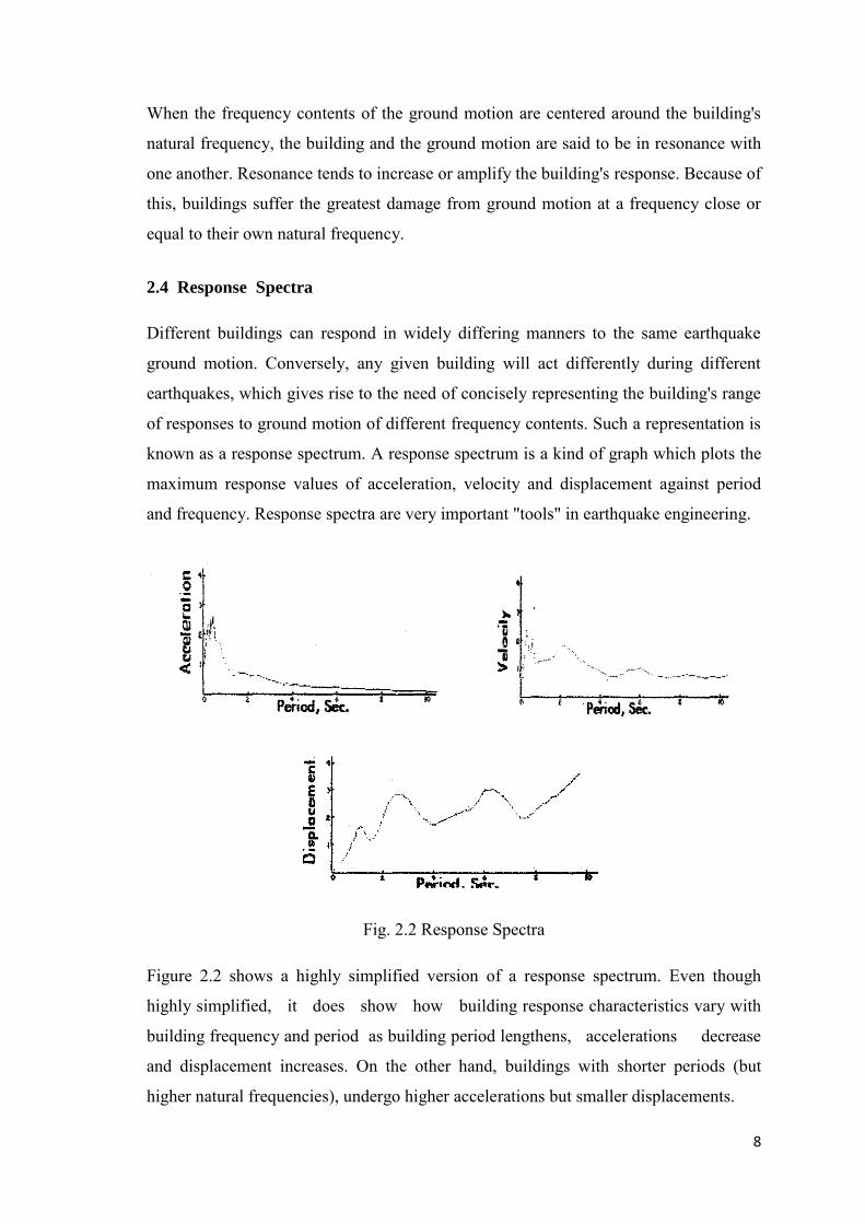
and frequency. Response spectra are very important "tools" in earthquake engineering.

Fig. 2.2 Response Spectra

Figure 2.2 shows a highly simplified version of a response spectrum. Even though

highly simplified, it does show how building response characteristics vary with

building frequency and period as building period lengthens, accelerations decrease

and displacement increases. On the other hand, buildings with shorter periods (but

higher natural frequencies), undergo higher accelerations but smaller displacements.

9

In the subsequent chapters, it will be described in more detail, the amount of

acceleration which a building undergoes during an earthquake is a critical factor in

determining how much damage it will suffer. The spectra described in figure 2.2

provides some indication of how accelerations are related to frequency characteristics

which shows one way in which response spectra can be useful, since identifying the

resonant frequencies at which a building will undergo peak accelerations is one very

important step in designing the building to resist earthquakes.

2.5 Analysis of Buildings Due to Earth Quake Forces

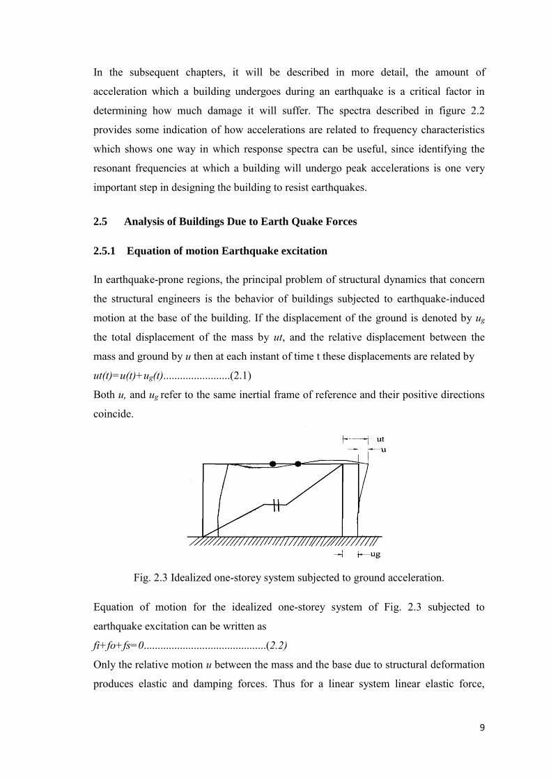
2.5.1 Equation of motion Earthquake excitation

In earthquake-prone regions, the principal problem of structural dynamics that concern

the structural engineers is the behavior of buildings subjected to earthquake-induced

motion at the base of the building. If the displacement of the ground is denoted by ug

the total displacement of the mass by ut, and the relative displacement between the

mass and ground by u then at each instant of time t these displacements are related by

ut(t)=u(t)+ug(t)........................(2.1)

Both u, and ug refer to the same inertial frame of reference and their positive directions

coincide.

Fig. 2.3 Idealized one-storey system subjected to ground acceleration.

Equation of motion for the idealized one-storey system of Fig. 2.3 subjected to

earthquake excitation can be written as

fi+fo+fs=0............................................(2.2)

Only the relative motion u between the mass and the base due to structural deformation

produces elastic and damping forces. Thus for a linear system linear elastic force,

10

fs=ku, damping force, fd=cu΄and inertia force f1 is related to the acceleration ϋ' of the

mass by f, = mϋ, Substituting these values to Equation 2.2,

mϋ + cu΄ + ku = -mϋg(t).......................(2.3)

This is the equation of motion governing the relative displacement or deformation u(t)

of the linear building of Fig. 2.3 subjected to a ground acceleration ϋ'g(t).

Dividing equation. 2.3 bym gives

ϋ + 2ζωnu΄+ ωn²u =mϋg(t)....................(2.4)

Where ωn is the natural circular frequency =√k/m

ζis the critical damping coefficient =c/2mωn

This is the basic equation of motion for a single degree of freedom system.

2.5.2 Code specified equivalent static load method

Equation 2.4 is identical to the idealized one-storied frame same as figure 2.3 subjected

to external dynamic force, P(t) which is

mϋ + cu΄ + ku = P(t).............................(2.5)

Comparing Eqs. 2.3 and 2.4 it is seen that the equation of motion for the building

subjected to two separate excitations - ground acceleration ϋg(t)and external force -

mϋg(t) are one and the same. Thus the relative displacement or deformation u(t) of the

building due to ground acceleration ϋg(t)will be identical to the displacement u(t) of the

building if its base werestationary and if it were subjected to an external force =-mϋg(t).

Thus the ground motion can therefore be replaced by the effective earthquake force

Peff(t)=-mϋg(t) .............................(2.6)

In this method the dynamic earthquake effect is represented by equivalent static load at

different levels. Earthquake load is a dynamic load. Due to earthquake load, a building

vibrates in different mode shapes and the load on the building, its intensities and

direction are dependent on the mode shapes.

For example, the figure 2.4 below shows first three fundamental modes of a shear type

building.

11

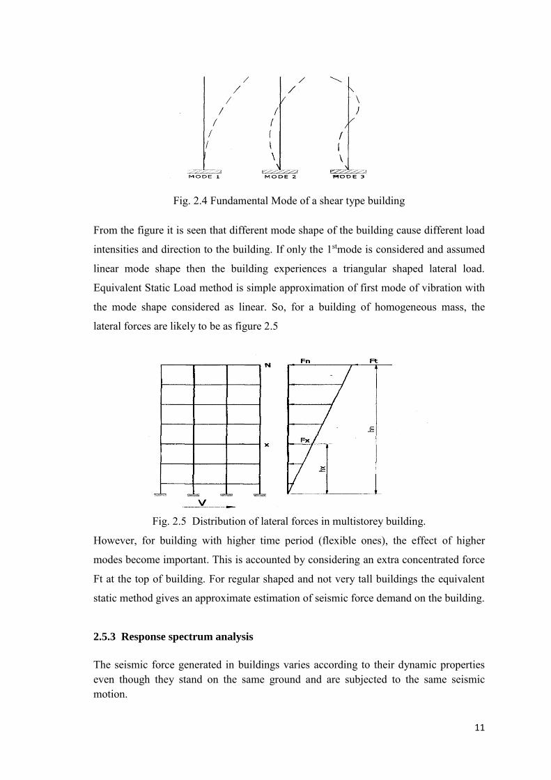
Fig. 2.4 Fundamental Mode of a shear type building

From the figure it is seen that different mode shape of the building cause different load

intensities and direction to the building. If only the 1stmode is considered and assumed

linear mode shape then the building experiences a triangular shaped lateral load.

Equivalent Static Load method is simple approximation of first mode of vibration with

the mode shape considered as linear. So, for a building of homogeneous mass, the

lateral forces are likely to be as figure 2.5

Fig. 2.5 Distribution of lateral forces in multistorey building.

However, for building with higher time period (flexible ones), the effect of higher

modes become important. This is accounted by considering an extra concentrated force

Ft at the top of building. For regular shaped and not very tall buildings the equivalent

static method gives an approximate estimation of seismic force demand on the building.

2.5.3 Response spectrum analysis

The seismic force generated in buildings varies according to their dynamic properties even though they stand on the same ground and are subjected to the same seismic motion.

12

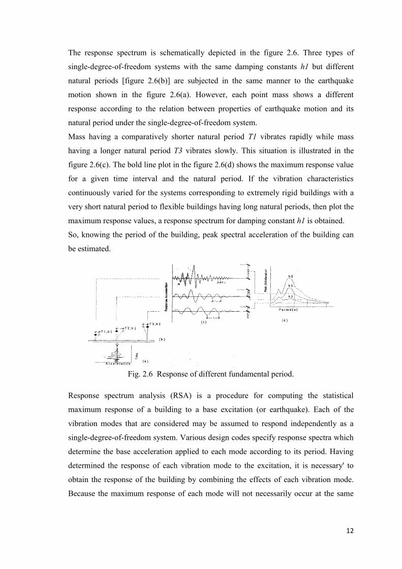
The response spectrum is schematically depicted in the figure 2.6. Three types of

single-degree-of-freedom systems with the same damping constants h1 but different

natural periods [figure 2.6(b)] are subjected in the same manner to the earthquake

motion shown in the figure 2.6(a). However, each point mass shows a different

response according to the relation between properties of earthquake motion and its

natural period under the single-degree-of-freedom system.

Mass having a comparatively shorter natural period T1 vibrates rapidly while mass

having a longer natural period T3 vibrates slowly. This situation is illustrated in the

figure 2.6(c). The bold line plot in the figure 2.6(d) shows the maximum response value

for a given time interval and the natural period. If the vibration characteristics

continuously varied for the systems corresponding to extremely rigid buildings with a

very short natural period to flexible buildings having long natural periods, then plot the

maximum response values, a response spectrum for damping constant h1 is obtained.

So, knowing the period of the building, peak spectral acceleration of the building can

be estimated.

Fig. 2.6 Response of different fundamental period.

Response spectrum analysis (RSA) is a procedure for computing the statistical

maximum response of a building to a base excitation (or earthquake). Each of the

vibration modes that are considered may be assumed to respond independently as a

single-degree-of-freedom system. Various design codes specify response spectra which

determine the base acceleration applied to each mode according to its period. Having

determined the response of each vibration mode to the excitation, it is necessary' to

obtain the response of the building by combining the effects of each vibration mode.

Because the maximum response of each mode will not necessarily occur at the same

13

instant, the statistical maximum response, where damping is zero, is taken as the square

root of the sum of the squares of the individual response.

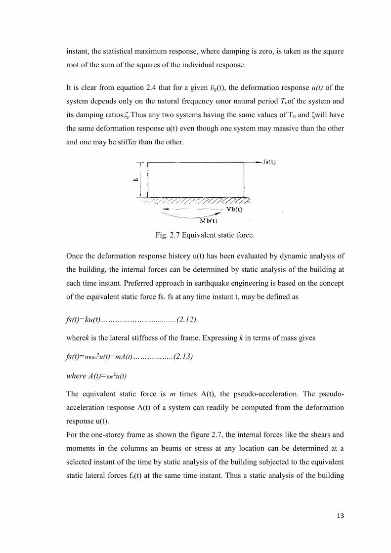
It is clear from equation 2.4 that for a given ϋg(t), the deformation response u(t) of the

system depends only on the natural frequency ωnor natural period Tnof the system and

its damping ratios,ζ.Thus any two systems having the same values of Tn and ζwill have

the same deformation response u(t) even though one system may massive than the other

and one may be stiffer than the other.

Fig. 2.7 Equivalent static force.

Once the deformation response history u(t) has been evaluated by dynamic analysis of

the building, the internal forces can be determined by static analysis of the building at

each time instant. Preferred approach in earthquake engineering is based on the concept

of the equivalent static force fs. fs at any time instant t, may be defined as

fs(t)=ku(t)…………………............(2.12) wherek is the lateral stiffness of the frame. Expressing k in terms of mass gives fs(t)=mωn²u(t)=mA(t)……………..(2.13) where A(t)=ωn²u(t) The equivalent static force is m times A(t), the pseudo-acceleration. The pseudo-

acceleration response A(t) of a system can readily be computed from the deformation

response u(t).

For the one-storey frame as shown the figure 2.7, the internal forces like the shears and

moments in the columns an beams or stress at any location can be determined at a

selected instant of the time by static analysis of the building subjected to the equivalent

static lateral forces fs(t) at the same time instant. Thus a static analysis of the building

14

would be necessary at each time instant when the responses are desired. In particular,

the base shear Vb(t) and the base over-turning moment Mb(t) are

Vb (t) = fs, (t) and Mb(t) = hfs(t) where h is the height of the mass above the base.

Putting the value of fs(t), one may get, Vb(t) = mA(t) and Mb(t) = hVb (t).

2.6 Earthquake Loading in the Light of BNBC

Bangladesh National Building Code was published in 2006 by Housing and Building

Research Institute. Like other building codes BNBC has different provisions for

calculation of earthquake load and analysis procedures for buildings subjected to

earthquake.

The BNBC, divides the country into three region of different possible earthquake

ground acceleration ranging from 0.075g to 0.25g. The Code also defines a simple

method to represent earthquake induced inertia forces by Equivalent Static Force for

static analysis. For dynamic analysis two methods are defined, namely

i. Response Spectrum Analysis and

ii. Time History Analysis.

2.6.1 Equivalent Static Load Method

In this method the dynamic earthquake effect is represented by an equivalent static load

at different levels proportion to mass at that level. Earthquake load is a dynamic load.

Due to earthquake load, a building vibrates in different mode shapes and load on the

building and its intensities and direction is dependent on the mode shapes. Equivalent

Static load method is an assumption of linear mode shape for the first mode of the

building. It is basically calculation of base shear from an earthquake load and its

comparison with the base shear capacity of the building.

2.6.2 Calculation of base shear

Total design base share, denoted by V, in a given direction is determined from the

following relation ………….……..(3.1)

The terms in the right hand side of the 3.1 may be explained as below

15

2.6.3 Zone coefficient, Z

This is the coefficient that represents the earthquake severity of the regions. Bangladesh

is divided into three zones of different earthquake severity. These are presented in table

A-13 in Appendix A.

The values of this coefficient is considered to represent the effective peak ground

acceleration (associated with an earthquake that has a 10% probability of being

exceeded in 50 years) expressed as a fraction of the acceleration due to gravity.

2.6.4 Structure importance coefficient, I

This is the coefficient that accounts the importance of building for post earthquake

activities. This coefficient is introduced from the experience of the previous

earthquakes when destruction of hospital and other important installation which has an

important role in post earthquake disaster management results in additional

'encumbrance. Now, some buildings like hospital, fire station, police station etc. are

designed giving more importance so that possibilities of these buildings to survive in

earthquake increase.

The earthquake lateral force is multiplied by some factor called Building Importance

Coefficient and are designed for a higher level of force so that the possibility of these

building being undamaged during an earthquake remains higher.

2.6.5 Seismic dead load, W

This is the seismic weight of the building that participates in earthquake response of the

building. This includes the self-weight of the building, other permanent dead load and

the part of the live load as prescribed by the Code defined in BNBC.

2.6.6 Response modification factor, R

Earthquake force is reduced by dividing this factor. This factor accounts the building's

ability to undergo inelastic deformation during earthquake. This factor depends on

building type, its damping properties and ductility. R is a measure ofthe capacity of the

structural system to absorb energy in the inelastic range through ductility and

redundancy. It is based primarily on the performance of similar systems in past

earthquakes. Different values of R are listed in BNBC/93.

16

2.6.7 Numeric coefficient, C

This is the coefficient that accounts for fundamental period of the building and soil

property of the building site.

C is calculated as C

where S is the Site coefficient depending on the characteristics of the soil at the site as

described in the Table 6.2.25 and T is the fundamental period of the building.

Fundamental period the building is calculated by some empirical formula as

T=Cthn3/4....................................................(3.3)

Where, hn = Total height of the building above the base.

Ct = a coefficient that depends on the building type and given in the code.

As it was discussed in the previous chapter, due to earthquake the building is subjected

to acceleration. This acceleration produces inertia force in the building. Applying

Newton's second law of motion, inertia force can be estimated by equation---

F = ma............................................................(3.4) Where m is the mass of the building

a is the ground acceleration.

Replacing the mass 'm' by one can get,

where, Z = ground acceleration in g.

This is the total force acting on the building.

Thus total base shear, V= WZ

Building deflects due to lateral force and this deflection absorbs some energy. How

much energy it absorbs, depend on the structural system, its damping properties etc. So,

the depending on the factors, the total force is reduced by dividing it by some factor, R

17

which is called the Response Modification factor. Value of R depends on the structural

system and is given in BNBC/93.

Further, the base shear is multiplied by a coefficient C called the Elastic Response

coefficient that account the fundamental period of the building and the soil property

under the building.

Thus with these coefficient, the equation of base shear becomes,

This base shear is distributed along the building height in a linear fashion mainly to

represent the first mode of deformation considering the first mode is linear.

2.7 Response Spectrum Method

BNBC recommends that response spectrum to be used in dynamic analysis shall be i. Site Specific Design Spectra A site specific response spectra shall be developed base

on the geologic, tectonic, seismologic, and soil characteristics associated with the

specific site.

ii. Normalized Response Spectra In absence of a site-specific response spectrum, the

normalized response spectra shall be used.

The response spectrum curves in the code are prepared for three different soil types and

5% of the critical damping. The ordinate represent the spectral acceleration and the

abscissa represents the natural period. Three soil types are defined in BNBC.

BNBC defines three normalized curves to be used in dynamic analysis performed using

Response Spectrum Analysis Method. The curve is shown below. In analysis

parameter, this curve to be modified as per specific site condition.

Fig. 2.8 Normalized Response Spectra of BNBC 2006.

18

BNBC does not provide any guideline for construction of Site Specific response

spectra.

2.8 Time History Analysis

Ground motion time history developed for the specific site shall be representative of

actual earthquake motions for an earthquake. Until recently, Bangladesh did not have

strong motion data recording centre. Few instruments for strong motion data recording

have been instrumented in Jamuna multi-purpose bridge and in Dhaka University.

2.9 Limitations of BNBC 2006 Though the code is comprehensive, few more details, in presentation even, could

enhance the acceptability of the code.

2.9.1 The zoning map

The code divides the country into three zones of different zoning coefficients with

marking only the districts. A detailed map as supplement would have been better for

the professionals to work with.

2.9.2 Structure period

Code defines 'Equivalent Static Load Method'- an alternate method to calculate

earthquake forces for regular buildings. In Equivalent Static Load Method, building

period is calculated as a function of building height. As a result, constant Base Shear in

all direction of the building is produced. Practically, building period is a function of

structural mass and stiffness. Unless the building is perfectly symmetric in both axes,

considerable change in building period may be found in other direction resulting

different base shear acting in that direction.

2.9.3 Base Shear Distribution

Unless the storey mass varies, the base shear distribution along the height of the

building is linear. Practically none of the fundamental mode shapes are linear. Many

codes, like current Uniform Building Code (UBC/2005), Indian Code (IS) etc.

recognizes non-linear distribution of base shear matching the 1st Fundamental mode

shape.

19

2.10 Seismic Strengthening

Retrofitting is technical interventions in structural system of a building that improve the

resistance to earthquake by optimizing the strength, ductility and earthquake loads.

Strength of the building is generated from the structural dimensions, materials, shape,

and number of structural elements, etc. Ductility of the building is generated from good

detailing, materials used, degree of seismic resistant, etc. Earthquake load is generated

from the site seismicity, mass of the buildings, important of buildings, degree of

seismic resistant, etc.

A retrofit strategy is a basic approach adopted to improve the probable seismic

performance of the building or otherwise reduce the existing risk to an acceptable level.

Both technical strategies and management strategies can be employed to obtain seismic

risk reduction. Technical strategies include such approaches as increasing building

strength, correcting critical deficiencies, altering stiffness, and reducing demand.

Management strategies include such approaches as change of occupancy, incremental

improvement and phased construction.

Engineers sometimes confuse systems and strategies. Strategies relate to modification

or control of the basic parameters that affect a building's earthquake performance.

These include the building's stiffness, strength, deformation capacity, and ability to

dissipate energy, as well as the strength and character of ground motion transmitted to

the building and the occupant and contents exposure within the building. Seismic risk

reduction strategies include such approaches as increasing strength, increasing stiffness,

increasing deformability, increasing damping, reducing occupancy exposure, and

modifying the character of the ground motion transmitted to the building. Strategies can

also include combinations of these approaches. Retrofit systems are specific methods

used to implement the strategy such as. For example, the addition of shear walls or

braced frames to increase stiffness and strength, the use of confinement jackets to

enhance deformability.

2.11 Retrofit Strategies

A wide range of technical and management strategies are available for reducing the

seismic risk inherent in an existing building. Technical strategies are approaches to

modifying the basic demand and response parameters of (Jhe building for the Design

Earthquake. These strategies include system completion, system strengthening, system

stiffening, and enhancing deformation capacity, enhancing energy dissipation capacity,

20

and reducing building demand.

2.11.1 Technical Strategies

As a building responds to earthquake ground motion, it experiences lateral

displacements and, in rum, deformations of its individual elements. At low levels of

response, the element deformations will be within their elastic (linear) range and no

damage will occur. At higher levels of response, element deformations will exceed their

linear elastic capacities and the building will experience damage. In order to provide

reliable seismic performance, a building must have a complete lateral force resisting

system, capable of limiting earthquake-induced lateral displacements to levels at which

the damage sustained by the building’s elements will be within acceptable levels for die

intended performance objective. The basic factors that affect the lateral force resisting

system’s ability to do this include the building’s mass, stiffness, damping, and

configuration; the deformation capacity of its elements; and die strength and character

of the ground motion it must resist.

Technical strategies can be grouped in the following categories

a) Building System Strengthening and stiffening

b) Enhancing Deformation capacity

c) Reducing Earthquake Demand

d) By Energy dissipation capacity

e) Controlling Lateral drift.

(a) Building system strengthening and stiffening

System strengthening and stiffening are the most common seismic performance

improvement strategies adopted for buildings with inadequate lateral force resisting

systems. The two are closely related but different. The effect of strengthening a

building is to increase the amount of total lateral force required to initiate damage

events within the building, if this strengthening is done without stiffening, then the

effect is to permit the building to achieve larger lateral displacements without damage.

System Strengthening and stiffening can be done by the following ways

Shear Walls: The introduction of shear walls into an existing concrete building is one

of the most commonly employed approaches to seismic upgrading. It is an extremely

effective method of increasing both building strength and stiffness. A shear wall system

21

is often economical and tends to be readily compatible with most existing concrete

buildings.

Fig. 2.9 RC Shear walls to resist lateral earthquake loads.

Fig. 2.10 RC shear wall layout a) unsymmetrical location not desirable b)symmetric layout desirable. Braced Frames: Braced steel frames are another common method of enhancing an

existing building's stiffness and strength. Typically, braced frames provide lower levels

of stiffness and strength than do shear walls, but they add far less mass to the building

than do shear walls, can be constructed with less disruption of the building, result in

less loss of light, and have a smaller effect on traffic patterns within the building.

Fig. 2.11 Braced steel frames.

22

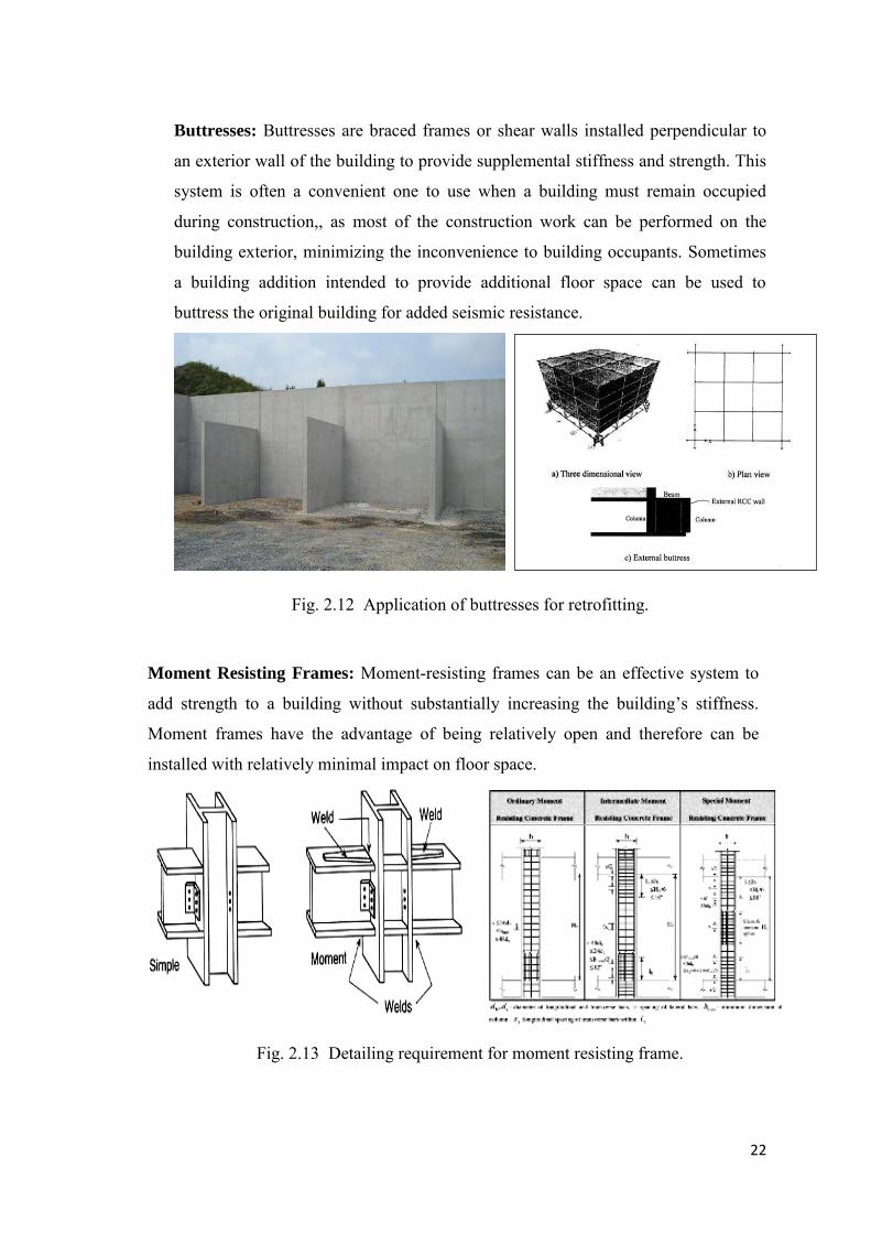
Buttresses: Buttresses are braced frames or shear walls installed perpendicular to

an exterior wall of the building to provide supplemental stiffness and strength. This

system is often a convenient one to use when a building must remain occupied

during construction,, as most of the construction work can be performed on the

building exterior, minimizing the inconvenience to building occupants. Sometimes

a building addition intended to provide additional floor space can be used to

buttress the original building for added seismic resistance.

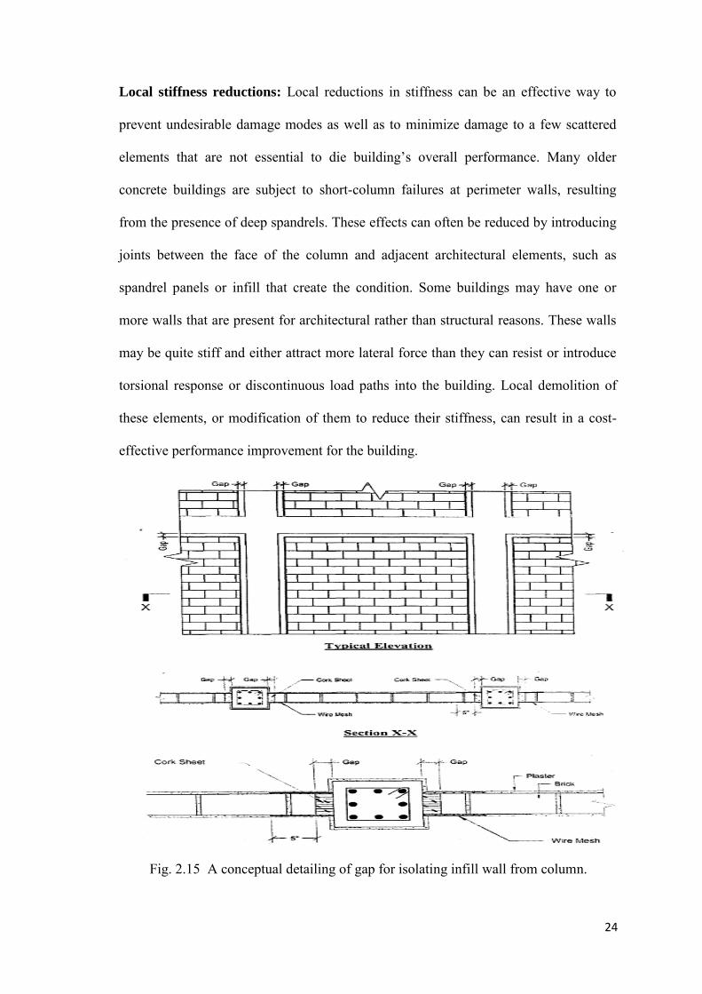
Fig. 2.12 Application of buttresses for retrofitting. Moment Resisting Frames: Moment-resisting frames can be an effective system to

add strength to a building without substantially increasing the building’s stiffness.

Moment frames have the advantage of being relatively open and therefore can be

installed with relatively minimal impact on floor space.

Fig. 2.13 Detailing requirement for moment resisting frame.

23

(b) Enhancing deformation capacity

Improvement in building seismic performance through enhancement of the ability of

individual elements within the building to resist deformations induced by the building

response is a relatively new method of seismic upgrading for concrete buildings. Some

of the methods for enhancing deformation capacity are discussed below

Adding Confinement The deformation capacity of nonductile concrete columns can be

enhanced through provision of exterior confinement jacketing. Jacketing may consist of

continuous steel plates encasing the existing element, reinforced concrete annuluses,

and fiber-reinforced plastic fabrics.

Confinement jacketing can improve the deformation capacity of concrete elements in

much the same way that closely spaced hoops in ductile concrete elements do. To be

effective, the jacketing material must resist the bursting pressure exerted by the existing

concrete element (under the influence of compressive stresses,) in a rigid manner.

Circular or oval jackets can provide the necessary confinement in an efficient manner

through the development of hoop stresses. Rectangular jackets tend to be less effective

and require cross ties in order to develop the required stiffness.

Fig. 2.14 Beam and column jacketing for an existing RCC strcture.

24

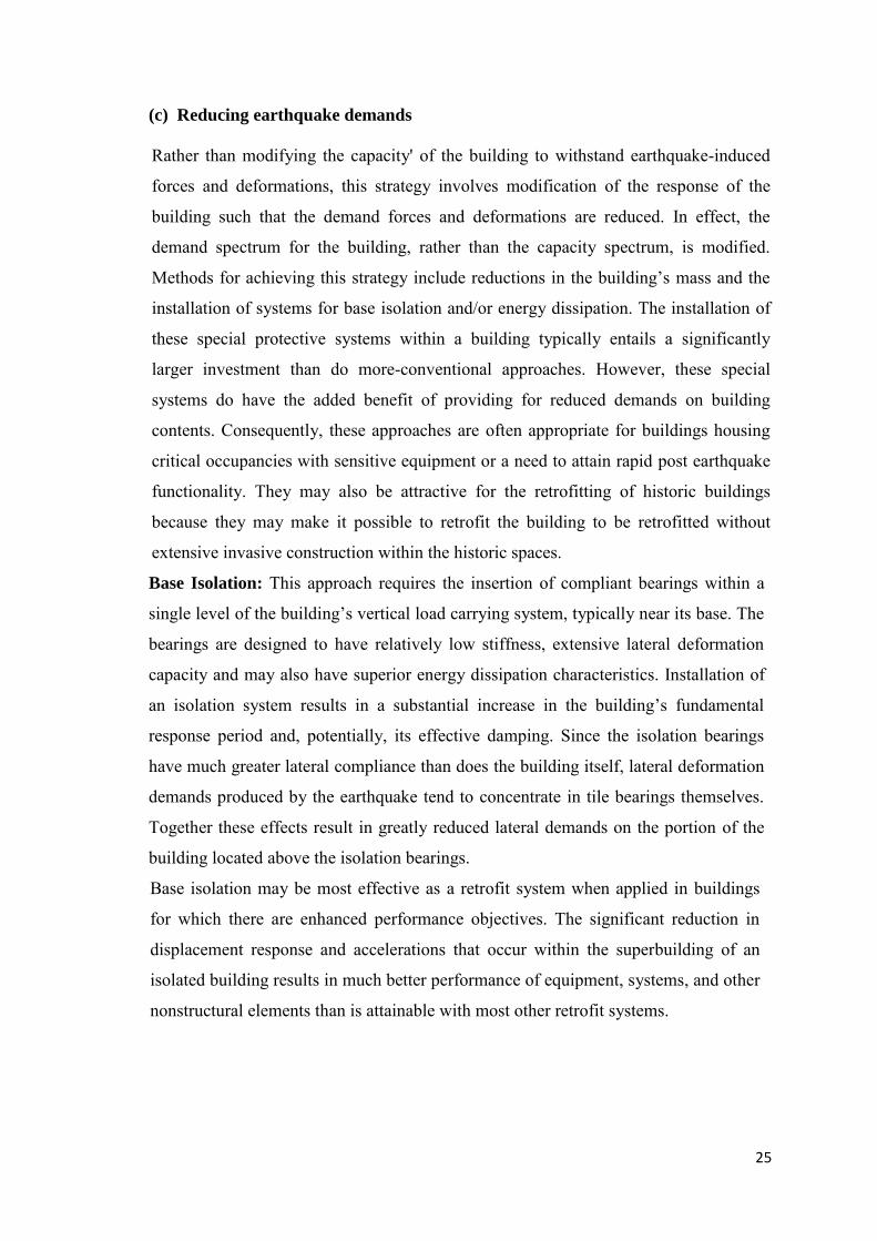
Local stiffness reductions: Local reductions in stiffness can be an effective way to

prevent undesirable damage modes as well as to minimize damage to a few scattered

elements that are not essential to die building’s overall performance. Many older

concrete buildings are subject to short-column failures at perimeter walls, resulting

from the presence of deep spandrels. These effects can often be reduced by introducing

joints between the face of the column and adjacent architectural elements, such as

spandrel panels or infill that create the condition. Some buildings may have one or

more walls that are present for architectural rather than structural reasons. These walls

may be quite stiff and either attract more lateral force than they can resist or introduce

torsional response or discontinuous load paths into the building. Local demolition of

these elements, or modification of them to reduce their stiffness, can result in a cost-

effective performance improvement for the building.

Fig. 2.15 A conceptual detailing of gap for isolating infill wall from column.

25

(c) Reducing earthquake demands

Rather than modifying the capacity' of the building to withstand earthquake-induced

forces and deformations, this strategy involves modification of the response of the

building such that the demand forces and deformations are reduced. In effect, the

demand spectrum for the building, rather than the capacity spectrum, is modified.

Methods for achieving this strategy include reductions in the building’s mass and the

installation of systems for base isolation and/or energy dissipation. The installation of

these special protective systems within a building typically entails a significantly

larger investment than do more-conventional approaches. However, these special

systems do have the added benefit of providing for reduced demands on building

contents. Consequently, these approaches are often appropriate for buildings housing

critical occupancies with sensitive equipment or a need to attain rapid post earthquake

functionality. They may also be attractive for the retrofitting of historic buildings

because they may make it possible to retrofit the building to be retrofitted without

extensive invasive construction within the historic spaces.

Base Isolation: This approach requires the insertion of compliant bearings within a

single level of the building’s vertical load carrying system, typically near its base. The

bearings are designed to have relatively low stiffness, extensive lateral deformation

capacity and may also have superior energy dissipation characteristics. Installation of

an isolation system results in a substantial increase in the building’s fundamental

response period and, potentially, its effective damping. Since the isolation bearings

have much greater lateral compliance than does the building itself, lateral deformation

demands produced by the earthquake tend to concentrate in tile bearings themselves.

Together these effects result in greatly reduced lateral demands on the portion of the

building located above the isolation bearings.

Base isolation may be most effective as a retrofit system when applied in buildings

for which there are enhanced performance objectives. The significant reduction in

displacement response and accelerations that occur within the superbuilding of an

isolated building results in much better performance of equipment, systems, and other

nonstructural elements than is attainable with most other retrofit systems.

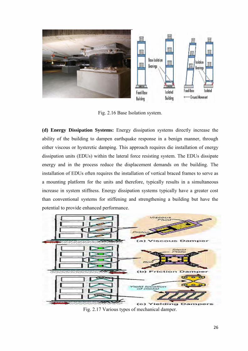
26

Fig. 2.16 Base Isolation system.

(d) Energy Dissipation Systems: Energy dissipation systems directly increase the

ability of the building to dampen earthquake response in a benign manner, through

either viscous or hysteretic damping. This approach requires die installation of energy

dissipation units (EDUs) within the lateral force resisting system. The EDUs dissipate

energy and in the process reduce the displacement demands on the building. The

installation of EDUs often requires the installation of vertical braced frames to serve as

a mounting platform for the units and therefore, typically results in a simultaneous

increase in system stiffness. Energy dissipation systems typically have a greater cost

than conventional systems for stiffening and strengthening a building but have the

potential to provide enhanced performance.

Fig. 2.17 Various types of mechanical damper.

27

Mass Reduction: The performance of some buildings can be greatly improved by

reducing the building mass. Building mass reductions reduce the building’s natural

period, the amount of inertial force that develops during its response and the total

displacement demand on the building. Mass can be reduced by removing heavy

nonstructural elements, such as cladding, water tanks and storage. In the extreme,

mass reduction can be attained by removing one or more building stories.

2.11.2 Management Strategies

Management strategies are programmatic in nature and are typically controlled by the

building owner rather than the design team. Management strategies tend to be of two

types strategies that affect the acceptability of the building’s probable performance and

strategies that regulate the way in which a technical strategy is implemented. They

include such approaches as occupancy change, demolition, temporary retrofit, phased

retrofit, retrofit while occupied, retrofit while vacant, exterior retrofit, and interior

retrofit. (a) Occupancy Change

Some buildings with inadequate performance capability for the current occupancy

may be an acceptable seismic risk if assigned other occupancies. The best risk

reduction approach for such buildings may simply be to alter the use of the building.

For example, a building capable of meeting the Substantial Life Safety performance

level, but not the Immediate Occupancy level would not be an acceptable risk for an

acute care facility at a hospital. It might be very adequate, however, for use as a day

care center or for medical offices. An appropriate strategy for such a situation may

be to use the existing building for one of these latter occupancies and construct a

new acute care facility. The desirability of this approach would obviously depend on

a number of factors, including a need for the building in the alternative use, the

availability of funding to construct a replacement facility, and the availability of

land.

28

2.12 Past Research On Seismic Performance Evaluation of Different

Retrofitting Schemes Using Non-Linear Analysis

Many studies have been conducted on seismic performance evaluation of different retrofitting schemes. The study (Huang et al. 2008) conducted a performance based evaluation and retrofit of

an existing hospital building in California, U.S. A nonlinear static pushover analysis as

described in FEMA 356, was used to evaluate the seismic performance of the existing

building. A seismic retrofit based on the pushover analysis was proposed and the

results showed that the life-safety target performance of the upgraded building was

achieved. In addition, the performance based retrofit scheme was compared to different

seismic retrofit scheme based on a prescriptive code design approach. The comparison

showed that the performance based approach lead to a better understanding of the

nonlinear behavior of the building during severe earthquakes and provided a more

efficient and cost effective strengthening solution for this building.

Another study (Gupta et al. 2015) highlighted the importance of adding shear wall in

increasing the lateral load carrying capacity of the building as well as the ductility. It’s

observed that the building before adding shear wall was not designed as earthquake

resistant. But after adding shear wall, significant improvement is seen in seismic

performance of the building. The columns which were failing before addition of shear

wall became safe after addition of shear wall. Also, the problem of soft story present

was solved. It’s suggested that as addition of shear wall imposes very less disturbance

to the existing building so it is still very viable option in improving the earthquake

resistance of the existing buildings.

Bilgin (2015) (Bilgin 2015) assessed the seismic performance evaluation of a typical

school building in accordance with the rules of Turkish Earthquake Code-2007. The

performance analysis was carried out by using nonlinear static analysis. The analytical

solutions showed that the intended performance level had not been satisfied for this

building and decided to retrofit the structural system. To strengthen the structural

system, shear walls were added in both directions. In order to find the economical

solution for the new strengthening system, nonlinear analyses are repeated with

29

different number of shear wall options. It’s observed that addition of shear walls

increases lateral load capacity and decreases displacement demands significantly.

Another study (Varum et al. 2013) highlighted the effectiveness of reinforced concrete

(RC) column jacketing for improving the seismic performance of existing RC building

buildings. Four three storey buildings with different structural configuration and

detailing were selected for seismic assessment and retrofitting purpose. The response of

buildings (original and retrofitted) was evaluated in terms of capacity curve and inter-

storey drift. The case studies also included the effect of P-delta effects and bi-axial

response of columns. The nature of the capacity curve represented the strong impact of

the P-delta effect, leading to a reduction of the global lateral stiffness and reducing the

strength of the building. Finally, a seismic safety assessment was performed based on

the drift limit proposed by FEMA-356. The assessment of original building buildings

indicated that they may exhibit inadequate seismic performance. However, RC column

jacketing highly improved seismic performance of all the buildings and mitigated

maximum drift demand within the drift limit proposed by FEMA-356.

The study (Akshara 2015) highlighted the need for performance based seismic

engineering in contrast to force-based design approaches. Four building performance

levels namely operational, immediate occupancy, life safety and collapse prevention

were studied in detail using FEMA 356 by conducting pushover analysis for an existing

five storied residential building. It’s observed that in performance based design, multi-

level seismic hazards were considered with an emphasis on the transparency of

performance objectives, thus ensuring better performance and minimum life-cycle cost.

Kumar et al. (2007) (Kumar et al. 2007) studied the usefulness of RC jacketing

technique to strengthen lightly reinforced beam-column joints experimentally. A full-

scale lightly reinforced concrete beam-column sub-assembly was strengthened by

casting an RC jacket outside the column and the joint, and the improvement brought

over by the retrofitting technique in the cyclic response of the specimen was verified

experimentally When subjected to cyclic lateral loading, The original specimen was

vulnerable to joint shear failure. On the other hand, the retrofitted specimen failed after

the formation of a plastic hinge in the beam, and the joint was no longer the weakest

component of the sub-assembly. It’s observed that Apart from the increase in the

30

capacity and deformability, the shear deformation of the joint panel reduced

significantly after retrofitting indicating that the RC jacketing method is effective in

strengthening non-seismic RC frames with inadequately reinforced joints.

Another study (Abd-Elhamed and Mahmoud 2017) investigated performance of a

residential 12-storey RC framed building, through pushover analysis, designed in

accordance with the Egyptian code following the (ATC 40) procedures using the well-

known software package ETABS. It’s observed that the plastic hinges started to occur

in beam ends and then the formation of these hinges started at columns of lower levels

before they extend to the upper level columns showing a strong column-weak beam

configuration. The analysis considered two levels of shakings. One of the chosen levels

fits the seismicity of Cairo zone and the other level is of higher magnitude. It has been

found from the analysis using level of shaking of intensity level that fits Cairo zone, the

demand curve intersects the capacity curve near the elastic zone. Consequently the

formed plastic hinges are always away from critical levels of performance and ensure

that the building behaves like the strong column-weak beam mechanism which

indicates that proposed model for nonlinear static analysis has produced satisfactory

behavior, better seismic performance and capability to sustain seismic loads fit code

requirements. However, exposing the framed building to seismic load exceeds twice the

one recommended by design code showed that the demand curve intersected the

capacity curve in the inelastic zone leading to formation of plastic hinges in the

dangerous level. Accordingly, the building behaves poorly and needs to be

strengthened to avoid severe damage or even collapse.

Leslie (2013) (Leslie 2013) explained the Pushover analysis in a simple way. He

mentioned that although elastic analysis gives a good indication of elastic capacity of

buildings and shows where yielding might first occur, it cannot account for

redistribution of forces during the progressive yielding that follows and predict its

failure mechanisms, or detect possibility and location of any premature failure. A non-

linear static analysis can predict these more accurately since it considers the inelastic

behavior of the building. It can help identify critical members likely to reach critical

states during an earthquake for which attention should be given during design and

detailing. Pushover analysis is a non-linear analysis procedure to estimate the strength

capacity of a building beyond its elastic limit (meaning Limit State) up to its ultimate

31

strength in the post-elastic range. In the process, the method also predicts potential

weak areas in the building, by keeping track of the sequence of damages of each and

every member in the building (generally known as ‘hinges’).He also pointed out some

of the major limitations of the PA such as the procedure basically takes into account

only the fundamental mode shape assuming it to be the predominant response and does

not consider effects of higher modes.

Giannopoulos (2009) (Giannopoulos 2009) investigated a typical five storey non-

ductile RC frame building which has been designed following past seismic regulations

in Greece has been analyzed using a nonlinear static (pushover) analysis. Few critical

sections are selected and the rotational ductility supply at various limit states as

predicted by FEMA 356 and Annex A of EC8 Part 3 (Eorocode 8) is calculated. The

two predictions are compared with each other and with results from the finite element

software analysis. The comparison demonstrates that there are differences in the results

produced by the two approaches and the results obtained from analysis provided useful

information for further development of Euro code 8.

The study (Inel and Ozmen 2006) pointed out the importance of user-defined nonlinear

hinge properties over default-hinge properties during pushover analysis. He mentioned

that studied the possible differences in the results of pushover analysis due to default

and user-defined nonlinear component properties. Four- and seven-story buildings are

considered to represent low- and medium- rise buildings for this study. Plastic hinge

length and transverse reinforcement spacing are assumed to be effective parameters in

the user-defined hinge properties. Observations showed that plastic hinge length and

transverse reinforcement spacing had no influence on the base shear capacity, while

these parameters had considerable effects on the displacement capacity of the frames.

Comparisons pointed out that an increase in the amount of transverse reinforcement

improves the displacement capacity. Although the capacity curve for the default-hinge

model is reasonable for modern code compliant buildings, it may not be suitable for

others. He concluded that the user-defined hinge model is better than the default-hinge

model in reflecting nonlinear behavior compatible with the element properties.

Lodi et al. (2011) (Lodi et al. 2011) discussed and illustrated the procedures to analyze

infill building with an example in ETABS, building analysis and design software by

32

Computers and Buildings, Inc. of a 2-D nonlinear static “pushover” analysis of a six

storey RC building with URM infill walls, based on guidelines and modeling

procedures given in the ATC-40 and FEMA-356 documents.

The study (Borkar and Pitale 2017) described the importance of performance based

analysis for soft storey building An existing open ground storey building with G+5

storey had been considered. Infill walls were modelled using procedure given in

FEMA. Non-linear static pushover analysis was done and studied effects of infill on

dynamic characteristics, yield patterns, seismic performance using finite element

software SAP 2000.It’s observed that the RC frame with open ground storey exhibited

very poor lateral strength stiffness and energy dissipation capacity due to formation of

shear hinges in ground storey columns under lateral load resulting uncontrolled

excessive deformation in the ground storey and need some retrofitting measures.

Hassaballa et al. (2014) (Hassaballa et al. 2014) mentioned the importance of

reinforced concreteshear walls in attaining the desired performance level of existing

hospital buildings in Sudan.

Another study (Naim and B. K Singh 2018) described the effectiveness of RC

Jacketing for seismic retrofitting of Buildings. In this case study, a G+3 storey RC

Building was considered for seismic analysis to calculate the additional seismic

strength of structural members like beams and columns. Based on this analysis

retrofitting measure RC Jacketing are suggested.

33

CHAPTER 3

CONCEPT OF PERFORMANCE BASED DESIGN

3.1 General

The primary objective of earthquake resistant design is to prevent building collapse

during earthquakes thus minimizing the risk of death or injury to people in or around

those buildings. The dynamic response of the building to earthquake ground motion is

the most important cause of earthquake-induced damage to building. The dynamic

nature of the response makes earthquake loadings markedly different from other

building loads. Through the careful selection of appropriate, well distributed lateral

load resisting systems, and by ensuring the building is reasonably regular in both plan

and elevation, the influence of many second order effects, such as torsional effects, can

be minimized and significant simplification can be made to model the dynamic

building response.

The traditional approach to seismic design of a building is a force-based design. The

design lateral forces on the building are determined using the response spectrum. In this

approach, there is no measure of the deformation capability of a member or of the

building. The performance based analysis is based on quantifying the deformations of

the members and the building as a whole, under the lateral forces of an earthquake of a

certain level of seismic hazard. The deformations or strains are better quantities to

assess damage than stress or forces. Since the deformations are expected to go beyond

the elastic values, a performance based analysis requires a nonlinear lateral load versus

deformation analysis. The performance based analysis give the analyst more choices of

'performance' of the building as compared to the limit states of collapse and

serviceability in a design based on limit state method.

3.2 Seismic Analysis Methods

There are different methods of seismic analysis which provide different degrees of

accuracy. The analysis process can be categorized on the basis of three factors the type

of the externally applied loads, the behavior of building/or structural materials and the

type of structural model selected. Based on the type of external action and behavior of

building, the analysis can be further classified as linear static analysis, linear dynamic

34

analysis, nonlinear static analysis, or non-linear dynamic analysis. Linear static analysis

or equivalent static analysis can only be used for regular building with limited height.

Linear dynamic analysis can be performed in two ways either by mode superposition

method or response spectrum method and elastic time history method. This analysis

will produce the effect of the higher modes of vibration and the actual distribution of

forces in the elastic range in a better way. They represent an improvement over linear

static analysis. The significant difference between linear static and dynamic analysis is

the level of force and their distribution along the height of the building. Non-linear

static analysis, which forms the basis of performance based design, is an improvement

over the linear static or dynamic analysis in the sense that it allows the inelastic

behavior of the building. The method still assumes a set of static incremental lateral

load over the height of building. The method is relatively simple to be implemented,

and provides information on the strength, deformation and ductility of the building and

the distribution of demands. These permits to identify critical members likely to reach

limit states during the earthquake, for which attention should be given during the

design and detailing process. But this method contains many limited assumptions,

which neglect the variation of loading patterns, the influence of higher modes, and the

effect of resonance. This method, under the name of push over analysis has acquired a

great deal of popularity now a days and in spite of these deficiencies this method

provides reasonable estimation of the global deformation capacity, especially for

buildings which primarily respond according to the first mode. A non-linear dynamic

analysis or inelastic time history analysis is the only method to describe the actual

behavior of the building during an earthquake. The method is based on the direct

numerical integration of the motion differential equations by considering the elasto-

plastic deformation of the building element. This method captures the effect of

amplification due to resonance, the variation of displacements at diverse levels of a

frame, an increase of motion duration and a tendency of regularization of movements

result as far as the level increases from bottom to top.

3.3 Methods to Perform Simplified Non Linear Analysis

Various analysis methods, both elastic (linear) and inelastic (nonlinear), are available

for the analysis of concrete buildings. Elastic analysis methods available include code

static lateral force procedures, code dynamic lateral force procedures and elastic

procedures using demand capacity ratios.

35

The most basic inelastic analysis method is the complete nonlinear time historey

analysis, which at this time is considered overly complex and impractical for general

use. Available simplified nonlinear method (ATC-40, 1996) [2] referred to as nonlinear

static analysis procedures, include the capacity spectrum method (CSM) that uses the

intersection of capacity (push over) curve and a reduced response spectrum to estimate

maximum displacement. Simplified nonlinear static analysis procedure using pushover

methods, such as the capacity spectrum method and the displacement co-efficient

method requires determination of three primary elements capacity, demand

(displacement) and performance. Each of these elements is briefly discussed below.

3.3.1 Capacity curve of a structure

The overall capacity of a building depends on the strength and deformation capacities

of the individual components of the building. In order to determine capacities beyond

the elastic limits, some form of nonlinear analysis such as the push over procedure, is

required. This procedure uses a series of sequential elastic analyses, superimposed to

approximate a force-displacement capacity diagram of the overall building. As the

loading progresses, the mathematical model of the building is modified to account for

reduced resistance of yielding components through insertion of plastic hinges. A lateral

force distribution is again applied until the additional components yield. This process is

continued until the building becomes unstable or until a predetermined limit is reached.

The push over capacity curve approximates how building behaves after exceeding their

elastic limit. Details of the procedure how a capacity curve is developed are presented

in section 3.4.

3.3.2 Demand curve of a structure

Ground motion during an earthquake produce complex horizontal displacement

patterns in buildings that may vary with time. Tracking this motion at every time-step

to determine structural design requirements is judged impractical. Traditional linear

analysis methods use lateral forces to represent a design condition. For nonlinear

methods it is easier and more direct to use a set of lateral displacements as a design

condition. For a given building and ground motion, the displacement demand is an

estimate of the maximum expected response of the building during the ground motion.

The displacement demand is established by use of the conventional response spectra-

36

by converting, it into Spectral Acceleration vs. Spectral Displacement format (Sec

3.4.1).

3.3.3 Performance point of a structure.

Once a capacity curve and demand displacement is defined, a performance check can

be done. A performance check verifies that structural and nonstructural components arc

not damaged beyond the acceptable limits of the performance objective for the forces

and displacement imposed by the displacement demand. Details of the procedure how

performance is ascertained are presented in section 3.4.1

3.4 Non Linear Static (Push Over) Analysis

As a building responds to earthquake ground motion, it experiences lateral

displacements and, in turn, imparts deformations to its individual elements. At low

levels of response, the element deformations will be within their elastic (linear) range

and no damage will occur. At higher levels of response, element deformations will

exceed their linear elastic capacities and the building will experience damage. In order

to provide reliable seismic performance, a building must have a complete lateral force

resisting system, capable of limiting earthquake-induced lateral displacements to levels

at which the damage sustained by the building's elements will be within acceptable

levels for the intended performance objective. The basic factors that affect the lateral

force resisting system's ability to do this include the building's mass, stiffness, damping

and configuration; the deformation capacity of its elements; and the strength and

character of the ground motion it must resist.

The nonlinear pushover analysis requires development of the capacity curve. The

capacity curve is derived from a nonlinear analysis for the building. In the process of

performing this incremental nonlinear static analysis, a capacity curve is developed for

the building. This capacity curve is simply the plot of the total lateral seismic demand

"V," on the building, at various increment of loading, against the lateral deflection of

the building at the roof level, under that applied lateral force. If a building had infinite

linear capacity, this capacity curve would be a straight line with a slope equal to the

global stiffness of the building. Since real building do not have the infinite linear

capacities, the capacity curve typically consists of a series of straight line segments

with decreasing slope, representing the progressive degradation in structural stiffness

that occurs as the building is subjected to increased lateral displacement, yielding and

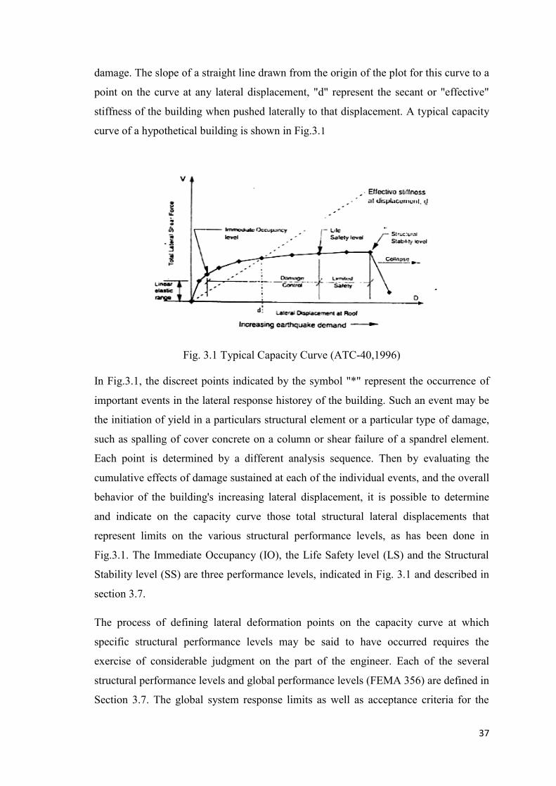
37

damage. The slope of a straight line drawn from the origin of the plot for this curve to a

point on the curve at any lateral displacement, "d" represent the secant or "effective"

stiffness of the building when pushed laterally to that displacement. A typical capacity

curve of a hypothetical building is shown in Fig.3.1

Fig. 3.1 Typical Capacity Curve (ATC-40,1996)

In Fig.3.1, the discreet points indicated by the symbol "*" represent the occurrence of

important events in the lateral response historey of the building. Such an event may be

the initiation of yield in a particulars structural element or a particular type of damage,

such as spalling of cover concrete on a column or shear failure of a spandrel element.

Each point is determined by a different analysis sequence. Then by evaluating the

cumulative effects of damage sustained at each of the individual events, and the overall

behavior of the building's increasing lateral displacement, it is possible to determine

and indicate on the capacity curve those total structural lateral displacements that

represent limits on the various structural performance levels, as has been done in

Fig.3.1. The Immediate Occupancy (IO), the Life Safety level (LS) and the Structural

Stability level (SS) are three performance levels, indicated in Fig. 3.1 and described in

section 3.7.

The process of defining lateral deformation points on the capacity curve at which

specific structural performance levels may be said to have occurred requires the

exercise of considerable judgment on the part of the engineer. Each of the several

structural performance levels and global performance levels (FEMA 356) are defined in

Section 3.7. The global system response limits as well as acceptance criteria for the

38

individual structural elements that make up typical buildings are described in section

3.8 to 3.9. These acceptance criteria generally consist of limiting values of element

deformation parameters, such as the plastic chord rotation of a beam or shear angle of a

wall. These limiting values have been selected as reasonable approximate estimates of

the average deformations at which certain types of element behavior such as cracking,

yielding, spalling, or crushing, may be expected to occur. As the incremental static

nonlinear analyses are performed, the engineer must monitor the cumulative

deformations of all important structural elements and evaluate them against the

acceptance criteria set before.

The point on the capacity curve at which the first element exceeds the permissible

deformation level for a structural performance level does not necessarily represent that

the building as a whole reaches that structural performance level. Most buildings

contain many elements and have considerable redundancy. Consequently, the onset of

unacceptable damage to a small percentage of these elements may not represent an

unacceptable condition with regard to the overall performance of the building. When

determining the points along the capacity curve for the building at which the various

structural performance level may said to be reached, the engineer must view the

performance of a building as whole and consider the importance of damage predicted

for the various elements on the overall behavior of the building.

The methodology described by ATC-40,1996 incorporates the concept of "Primary"

and "Secondary" elements to assist the engineers in making these judgments. Primary

elements are those that are required as part of the lateral force resisting system for the

building. All the other elements are designated as secondary elements. For a given

performance level, secondary elements are generally permitted to sustain more damage

than primary elements since degradation of secondary elements does not have a

significant effect on the lateral load resisting capability of the building. If in the

development of the capacity curve it is determined that a few element fail to meet the

acceptance criteria for a given performance level at an increment of lateral loading and

displacement, the engineer has the ability to designate these nonconforming elements as

secondary, enabling the use of more liberal acceptance criteria for these few elements.

Care is exercised not to designate an excessive number of elements that are effective in

resisting lateral force as secondary (ATC-40, 1996).

39

3.4.1 Capacity Spectrum Method

The capacity spectrum method, a nonlinear static procedure, provides a graphical

representation of the global force-displacement capacity curve of the building (i.e.

pushover curve) and compares it to the response spectra representations of the

earthquake demand. This method is a very useful tool in the evaluation and retrofit

design of existing concrete buildings. The graphical representation provides a clear

picture of how a building responds to earthquake ground motion, and, as illustrated

below, it provides an immediate and clear picture of how various retrofit strategies,

such as adding stiffness or strength, will affect the building's response to earthquake

demands.

The capacity spectrum curve for the building is obtained by transforming the capacity

curve from lateral force (V) vs. lateral displacement (d) coordinates to spectral

acceleration (Sa) vs. spectral displacement (Sa) coordinates using the modal shape

vectors, participation factors and modal masses obtained from a modal analysis of the

building. In order to compare the Building's capacity to the earthquake demand, it is

required to plot the response spectrum and the capacity spectrum on the same plot. The

conventional response spectrum plotted in spectral acceleration vs. period coordinate

has to be changed in to spectral acceleration vs. spectral displacement coordinate. This

form of response spectrum is known asacceleration displacement response spectrum

(ADRS). The details of the procedure for conversion of conventional response spectra

to ADRS and capacity curve to capacity spectrum are provided in Appendix-A.

3.4.2 Displacement Coefficient Method

Another procedure for calculating demand displacement is Displacement Coefficient

Method which provides a direct numerical process for calculating the displacement

demand. Details of displacement Coefficient Method is available in ATC-40, 1996.

Performance analysis of the buildings under this thesis was made using Capacity

Spectrum Method.

3.5 Seismic Performance Evaluation

The essence of virtually all seismic evaluations procedures is a comparison between

some measures of the "demand" that earthquake place on building to a measure of the

40

"capacity" of the building to resist the induced effects. Traditional design procedures

characterize demand and capacity as forces. Base shear (total horizontal force at the

lowest level of the building) is the normal parameter that is used for this purpose. The

base shear demand that would be generated by a given earthquake, or intensity of

ground motion is calculated, and compares this to the base shear capacity of the

building. If the building were subjected to a force equal to its base shear capacity some

deformation and yielding might occur in some structural elements, but the building

would not collapse or reach an otherwise undesirable overall level of damage. If the

demand generated by the earthquake is less than the capacity then the design is deemed

acceptable.

The first formal seismic design procedures recognized that the earthquake accelerations

would generate forces proportional to the weight of the building. Over the years,

empirical knowledge about the actual behavior of real buildings in earthquakes and

theoretical understanding of structural dynamics advanced. The basic procedure was

modified to reflect the fact that the demand generated by the earthquake accelerations

was also a function of the stiffness of the building.The inherently better behavior of

some buildings over others have also been begun to be recognized. Consequently, the

reduced seismic demand has been assumed for some building based on the

characteristics of the basic structural material and system. The motivation to reduce

seismic demand for design came because it could not be rationalized theoretically how

buildings resisted the forces generated by earthquakes. This was partially the result of

the fundamental assumption that buildings resisted loads linearly without yielding or

permanent structural deformation.

3.6 Nonlinear Static Procedure for Capacity Evaluation of Structures

Instead of comparing forces, nonlinear static procedures use displacements to compare

seismic demand to the capacity of a building. This approach included consideration of

the ductility of the building on an element by element basis. The inelastic capacity of a

building is then a measure of its ability to dissipate earthquake energy. The current

trend in seismic analysis is toward these simplified inelastic procedures.

The recommended central methodology is on the formulation of inelastic capacity

curve for the building. This curve is a plot of the horizontal movement of a building as

it is pushed to one side. Initially the plot is a straight line as the building moves

linearly. As the parts of the building yield the plot begins to curve as the building

41

softens. This curve is generated by building a model of the entire building from

nonlinear representations of all of its elements and components. Most often this is

accomplished with a computer and structural analysis software. The specific forces and

displacement characteristics are specified for each piece of the building resisting the

earthquake demand. These pieces are assembled geometrically to represent the

complete lateral load resisting system. The resulting model is subjected to increasing

increment of load in a pattern determined by its dynamic properties. The corresponding

displacements define the inelastic capacity curve of the building. The generation of the

capacity curve defines the capacity of the building uniquely and independently of any

specific seismic demand. In this sense it replaces the base shear capacity of

conventional procedures. When an earthquake displaces the building laterally, its

response is represented by a point on this curve. A point on the curve defines a specific

damage state of the building, since the deformation of its entire components can be

related to the global displacement of the building.

The capacity of a particular building and the demand imposed upon it by a given

earthquake motion are not independent. One source of this mutual dependence is

evident from the capacity curve itself. As the demand increases the building eventually

yields and, as its stiffness decreases, its period lengthens. Since the seismic

accelerations depend on period, demand also changes as the building yields. Another

source of mutual dependence between capacity and demand is effective damping. As

building yields in response to seismic demand, it dissipates energy with hysteretic

damping. Building that have large, stable hysteretic loops during cyclic yielding

dissipate more energy than those with pinched loops caused by degradation of strength

and stiffness. Since the energy that is dissipated need not be stored in the building, the

damping has the effect of diminishing displacement demand.

3.7 Structural Performance Levels and Ranges

The performance of a building under any particular event is dependent on a wide range

of parameters. These parameters are defined (ATC-40, 1996; FEMA 356, 2000)

qualitatively in terms of the safety afforded by the building to the occupants during and

after the event; the cost and feasibility of restoring the building to pre-earthquake

condition; the length of time the building is removed from service to effect repairs; and

economic, architectural, or historic impacts on the larger community. These

42

performance characteristics are directly related to the extent of damage that would be

sustained by the building.

The Federal Emergency Management Agency in its report 'Prestandard and

Commentary for the Seismic Rehabilitation of Buildings, (FEMA-356, 2000) defines

the structural performance level of a building to be selected from four discrete

structural performance levels and two intermediate structural performance ranges. The

discrete Structural Performance Levels are

• Immediate Occupancy (S-1)

• Life Safety (S-3)

• Collapse Prevention (S-5), and • Not Considered (S-6).

The intermediate Structural Performance Ranges are the

• Damage Control Range (S-2) and the

• Limited Safety Range (S-4)

The definition of these performance ranges are given by FEMA (FEMA-356, 2000).

Acceptance criteria for performance within the Damage Control Structural Performance

Range may be obtained by interpolating the acceptance criteria provided for the

Immediate Occupancy and Life Safety Structural Performance Levels. Acceptance

criteria for performance within the Limited Safety Structural Performance Range may

be obtained by interpolating the acceptance criteria provided for the Life Safety and

Collapse Prevention Structural Performance Levels. The performance levels and

ranges, as per FEMA (FEMA-356, 2000), are described in the sections that follow.

3.7.1 Immediate occupancy structural performance level (S-1) Structural Performance Level S-1, Immediate Occupancy, may be defined as the post-

earthquake damage state of a building that remains safe to occupy, essentially retains

the pre-earthquake design strength and stiffness of the building, and is in compliance

with the acceptance criteria specified in this standard for this Structural Performance

Levels defined at Tables B1-B3 in FEMA-356, 2000 (Appendix-B).

Structural Performance Level S-1, Immediate Occupancy, means the post-earthquake

damage state in which only very limited structural damage has occurred.

43

The basic vertical and lateral-force-resisting systems of the building retain nearly all of

their pre-earthquake strength and stiffness. The risk of life-threatening injury as a result

of structural damage is very low, and although some minor structural repairs may be

appropriate, these would generally not be required prior to re-occupancy.

3.7.2 Damage control structural performance range (S-2)

Structural Performance Range S-2, Damage Control, may be defined as the continuous

range of damage states between the Life Safety Structural Performance Level (S-3) and

the Immediate Occupancy Structural Performance Level (S-l) defined at Tables B1-B3

in FEMA-356, 2000 (Appendix-B).

Design for the Damage Control Structural Performance Range may be desirable to

minimize repair time and operation interruption, as a partial means of protecting

valuable equipment and contents, or to preserve important historic features when the

cost of design for immediate occupancy is excessive.

3.7.3 Life safety structural performance level (S-3) Structural Performance Level S-3, Life Safety, shall be defined as the post-earthquake

damage state that includes damage to structural components but retains a margin

against onset of partial or total collapse in compliance with the acceptance criteria

specified in FEMA for this Structural Performance Level defined at tables B1-B3 in

FEMA-356, 2000 (Appendix-B).

Structural Performance Level S-3, Life Safety, means the post-earthquake damage state

in which significant damage to the building has occurred, but some margin against

either partial or total structural collapse remains. Some structural elements and

components are severely damaged, but this has not resulted in large falling debris

hazards, either within or outside the building. Injuries may occur during the earthquake;

however, the overall risk of life-threatening injury as a result of structural damage is

expected to be low. It should be possible to repair the building; however, for economic

reasons this may not be practical. While the damaged building is not an imminent

collapse risk, it would be prudent to implement structural repairs or install temporary

bracing prior to re-occupancy.

44

3.7.4 Limited safety structural performance range (S-4) Structural Performance Range S-4, Limited Safety, may be defined as the continuous

range of damage states between the Life Safety Structural Performance Level (S-3) and

the Collapse Prevention Structural Performance Level (S-5) defined at tables B1-B3 in

FEMA-356, 2000 (Appendix-B).

3.7.5 Collapse prevention structural performance level (S-5) Structural Performance Level S-5, Collapse Prevention, may be defined as the post-

earthquake damage state that includes damage to structural components such that the

building continues to support gravity loads but retains no margin against collapse in

compliance with the acceptance criteria specified in FEMA for this Structural

Performance Level defined at tables B1-B3 in FEMA-356, 2000 (Appendix-B).

Structural Performance Level S-5, Collapse Prevention, means the post-earthquake

damage state in which the building is on the verge of partial or total collapse.

Substantial damage to the building has occurred, potentially including significant

degradation in the stiffness and strength of the lateral-force resisting system, large

permanent lateral deformation of the building, and to a more limited extent degradation

in vertical-load-carrying capacity. However, all significant components of the gravity

load resisting system must continue to carry their gravity load demands. Significant risk

of injury due to falling hazards from structural debris may exist. The building may not

be technically practical to repair and is not safe for re-occupancy, as aftershock activity

could induce collapse.

3.8 Target Building Performance Levels

Building performance is a combination of the both structural and nonstructural

components. Tables B1-B3(Appendix-B) in FEMA-356, 2000 describe the

approximate limiting levels of structural damage that may be expected of buildings

evaluated to the levels defined for a target seismic demand. These tables represent the

physical states of mathematical calculation of different performance levels.

45

3.9 Response Limits

To determine whether a building meets a specified performance objective, response

quantities from a nonlinear analysis are compared with limits given for appropriate

performance levels (ATC-40, 1996 and FEMA-356, 2000). The response limits fall into

two categories (i) Global Building Acceptability Limits and (ii) Element and

Component Acceptability Limits. These are described next.

3.9.1 Global building acceptability limits

These response limits include requirements for the vertical load capacity, lateral load

resistance, and lateral drift. Table B4 (Appendix-B) gives the limiting values as per

ATC-40 for different performance levels. These are described below.

3.9.1.1 Gravity Load

The gravity load capacity of the building building must remain intact for acceptable

performance at any level. Where an element or component loses capacity to support

gravity loads, the building must be capable of redistributing its load to other elements

or components of the existing system.

3.9.1.2 Lateral Load

Some component types are subjected to degrading over multiple load cycles. If a

significant number of components degrade, the overall lateral force resistance of the

building may be affected. The lateral load resistance of the building system, including

resistance to the effects of gravity loads acting through lateral displacements, should

not degrade by more than 20 percent of the maximum resistance of the building for the

extreme case.

Two effects can lead to loss of lateral load resistance with increasing displacement. The

first is gravity loads acting through lateral displacements, known as the P-∆ effect. The

P-∆ effect is most prominent for flexible buildings with little redundancy and low

lateral load strength relative to the building's weight. The second effect is degradation

in resistance of individual components of the building under the action of reversed

deformation cycles. When lateral load resistance of the building degrades with

46

increasing displacement, there is a tendency for displacements to accumulate in one

direction. This tendency is especially important for long-duration events.

Table B4 in ATC-40,1996(Appendix-B) gives the deformation drift limits for different

performance level. Maximum total drift is defined as the inter-storey drift at the

performance point displacement. Maximum inelastic drift is defined as the portion of

the maximum total drift beyond the effective yield point. For Structural Stability, the

maximum total drift in storey i at the performance point should not exceed the quantity

0.33 where Vi is the total calculated shear force in storey i and Pi is the total gravity

load (i.e. dead plus likely live load) at storey i(ATC-40, 1996).

3.9.2 Element and component acceptability limits

It can be divided in two categories.

3.9.2.1 Primary and secondary elements and components

Each element and component is classified as primary or secondary depending on its

significance to the lateral load resisting system at or near the performance point.

Elements and components that provide a significant portion of the building's strength or

lateral stiffness at the performance point are considered primary. Other elements and

components may be considered secondary (ATC-40, 1996).

3.9.2.2 Deformation of force controlled action

All structural actions may be classified (FEMA-356, 2000) as either deformation

controlled or force-controlled using the component force versus deformation curves

shown in Fig. 3.2. The Type 1 curve depicted in Fig. 3.2 is representative of ductile

behavior where there is an elastic range (point 0 to point 1 on the curve) followed by a

plastic range (points 1 to 3) with non-negligible residual strength and ability to support

gravity loads at point 3. The plastic range includes a strain hardening or softening range

(points 1 to 2) and a strength-degraded range (points 2 to 3). Primary component

actions exhibiting this behavior shall be classified as deformation-controlled if the

strain-hardening or strain-softening range is such that e > 2g; otherwise, they shall be

classified as force controlled. Secondary component actions exhibiting Type 1 behavior

shall be classified as deformation-controlled for any e/g ratio. The Type 2 curve

depicted in Fig. 3.2 is representative of ductile behavior where there is an elastic range

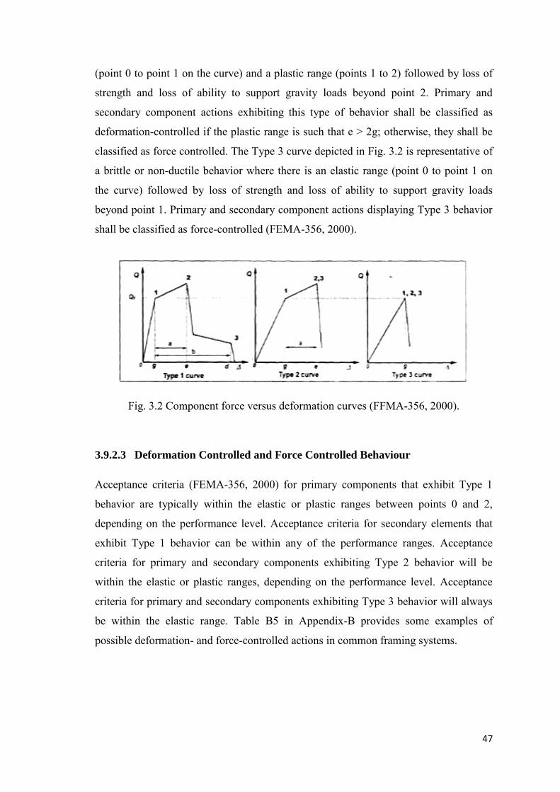
47

(point 0 to point 1 on the curve) and a plastic range (points 1 to 2) followed by loss of

strength and loss of ability to support gravity loads beyond point 2. Primary and

secondary component actions exhibiting this type of behavior shall be classified as

deformation-controlled if the plastic range is such that e > 2g; otherwise, they shall be

classified as force controlled. The Type 3 curve depicted in Fig. 3.2 is representative of

a brittle or non-ductile behavior where there is an elastic range (point 0 to point 1 on

the curve) followed by loss of strength and loss of ability to support gravity loads

beyond point 1. Primary and secondary component actions displaying Type 3 behavior

shall be classified as force-controlled (FEMA-356, 2000).

Fig. 3.2 Component force versus deformation curves (FFMA-356, 2000).

3.9.2.3 Deformation Controlled and Force Controlled Behaviour

Acceptance criteria (FEMA-356, 2000) for primary components that exhibit Type 1

behavior are typically within the elastic or plastic ranges between points 0 and 2,

depending on the performance level. Acceptance criteria for secondary elements that

exhibit Type 1 behavior can be within any of the performance ranges. Acceptance

criteria for primary and secondary components exhibiting Type 2 behavior will be

within the elastic or plastic ranges, depending on the performance level. Acceptance

criteria for primary and secondary components exhibiting Type 3 behavior will always

be within the elastic range. Table B5 in Appendix-B provides some examples of

possible deformation- and force-controlled actions in common framing systems.

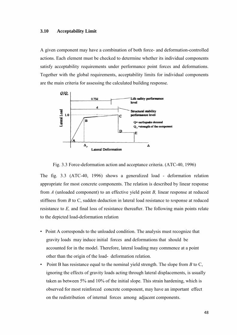
48

3.10 Acceptability Limit

A given component may have a combination of both force- and deformation-controlled

actions. Each element must be checked to determine whether its individual components

satisfy acceptability requirements under performance point forces and deformations.

Together with the global requirements, acceptability limits for individual components

are the main criteria for assessing the calculated building response.

Fig. 3.3 Force-deformation action and acceptance criteria. (ATC-40, 1996)

The fig. 3.3 (ATC-40, 1996) shows a generalized load - deformation relation

appropriate for most concrete components. The relation is described by linear response

from A (unloaded component) to an effective yield point B, linear response at reduced

stiffness from B to C, sudden deduction in lateral load resistance to response at reduced

resistance to E, and final loss of resistance thereafter. The following main points relate

to the depicted load-deformation relation

• Point A corresponds to the unloaded condition. The analysis must recognize that

gravity loads may induce initial forces and deformations that should be

accounted for in the model. Therefore, lateral loading may commence at a point

other than the origin of the load- deformation relation.

• Point B has resistance equal to the nominal yield strength. The slope from B to C,

ignoring the effects of gravity loads acting through lateral displacements, is usually

taken as between 5% and 10% of the initial slope. This strain hardening, which is

observed for most reinforced concrete component, may have an important effect

on the redistribution of internal forces among adjacent components.

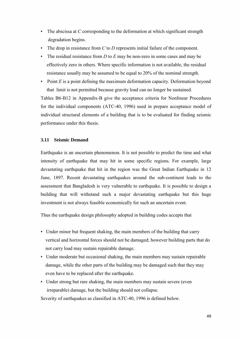
49

• The abscissa at C corresponding to the deformation at which significant strength

degradation begins.

• The drop in resistance from C to D represents initial failure of the component.

• The residual resistance from D to E may be non-zero in some cases and may be

effectively zero in others. Where specific information is not available, the residual

resistance usually may be assumed to be equal to 20% of the nominal strength.

• Point E is a point defining the maximum deformation capacity. Deformation beyond

that limit is not permitted because gravity load can no longer be sustained.

Tables B6-B12 in Appendix-B give the acceptance criteria for Nonlinear Procedures

for the individual components (ATC-40, 1996) used in prepare acceptance model of

individual structural elements of a building that is to be evaluated for finding seismic

performance under this thesis.

3.11 Seismic Demand

Earthquake is an uncertain phenomenon. It is not possible to predict the time and what

intensity of earthquake that may hit in some specific regions. For example, large

devastating earthquake that hit in the region was the Great Indian Earthquake in 12

June, 1897. Recent devastating earthquakes around the sub-continent leads to the

assessment that Bangladesh is very vulnerable to earthquake. It is possible to design a

building that will withstand such a major devastating earthquake but this huge

investment is not always feasible economically for such an uncertain event.

Thus the earthquake design philosophy adopted in building codes accepts that

• Under minor but frequent shaking, the main members of the building that carry

vertical and horizontal forces should not be damaged; however building parts that do

not carry load may sustain repairable damage.

• Under moderate but occasional shaking, the main members may sustain repairable

damage, while the other parts of the building may be damaged such that they may

even have to be replaced after the earthquake.

• Under strong but rare shaking, the main members may sustain severe (even

irreparable) damage, but the building should not collapse.

Severity of earthquakes as classified in ATC-40, 1996 is defined below.

50

3.11.1 The serviceability earthquake (SE) The Serviceability Earthquake (SE) is defined probabilistically as the level of ground

shaking that has a 50 percent chance of being exceeded in 50-year period. This level of

earthquake ground shaking is typically about 0.5 times of the level of ground shaking

of the Design Earthquake. The SE has a mean return period of approximately 75 years.

Damage in the non structural elements is expected during Serviceability Earthquake.

3.11.2 The design earthquake (DE)

The Design Earthquake (DE) is defined probabilistically as the level of ground shaking

that has a 10 percent chance of being exceeded in a 50-year period. The DE represents

an infrequent level of ground shaking that can occur during the life of the building. The

DE has a mean return period of approximately 500 years. Minor repairable damage in

the primary lateral load carrying system is expected during Design Earthquake. For

secondary elements, the damage may be such that they require replacement.

3.11.3 The maximum earthquake (ME)

The Maximum Earthquake (ME) is defined deterministically as the maximum level of

earthquake ground shaking which may ever be expected at the building site within the

known geologic frame work. In probabilistic terms, the ME has a return period of about

1,000 years. During Maximum Earthquake, buildings will be damaged beyond

repairable limit but will not collapse.

3.12 Development of Elastic Site Response Spectra

Elastic response spectra for a site are based on estimate of Seismic Coefficient, CA

which represents the effective peak acceleration (EPA) of the ground and Cv which

represents 5 percent-damped response of a 1-second system. These coefficients for a

particular zone are dependent on the seismicity of the area, the proximity of the site to

active seismic sources, and site soil profile characteristics.

51

3.12.1 Seismic zone

Bangladesh is divided into three seismic zones as per BNBC. Table B13 in

BNBC,2006(Appendix-B) shows the values of zone coefficients of Bangladesh.

3.12.2 Seismic Source Type

As per ATC-40 (1996), three types of seismic source may be defined as shown in Table B14 in ATC-40,1996(Appendix-B)

3.12.3 Near Source Factor

Currently data pertaining to the active faults close to Dhaka city is not available. It is

not possible to estimate the seismic source distance from a specific site being

considered in this thesis. But for the analysis of the buildings considered in this thesis,

it may be safely assumed that all the sources are located at distance more than 15 km

and the Table B15 in ATC-40,1996 (Appendix-B) may be used to neglect the Near-

Source effects for the present study.

3.12.4 Seismic Coefficients

For each earthquake hazard level, the building is assigned a seismic coefficient CAin

accordance Table B16 in ATC-40,1996 (Appendix-B) and a seismic coefficient Cv in

accordance with Table B17 in ATC-40,1996 (Appendix-B). Seismic coefficient CA

represents the effective peak acceleration (EPA) of the ground. A factor of about 2.5

times CA represents the average value of peak response of a 5 percent-damped short-

period system in the acceleration domain. The seismic coefficient Cv represents 5

percent-damped response of a 1-second system. Cv divided by period (T) defines

acceleration response in the velocity domain. These coefficients are dependent on soil

profile type and the product of earthquake zoning coefficient-Z, severity of earthquake-

E and near source factor-N (ZEN). The soil profile types are classified in Table B18 in

ATC-40,1996(Appendix-B).

3.13 Element Hinge Property

It is known that reinforced concrete does not respond elastically to load level about half

the ultimate value. When an element is stressed beyond its elastic limit, due to inelastic

deformation of the materials, the element will continue to deform disproportionate to its

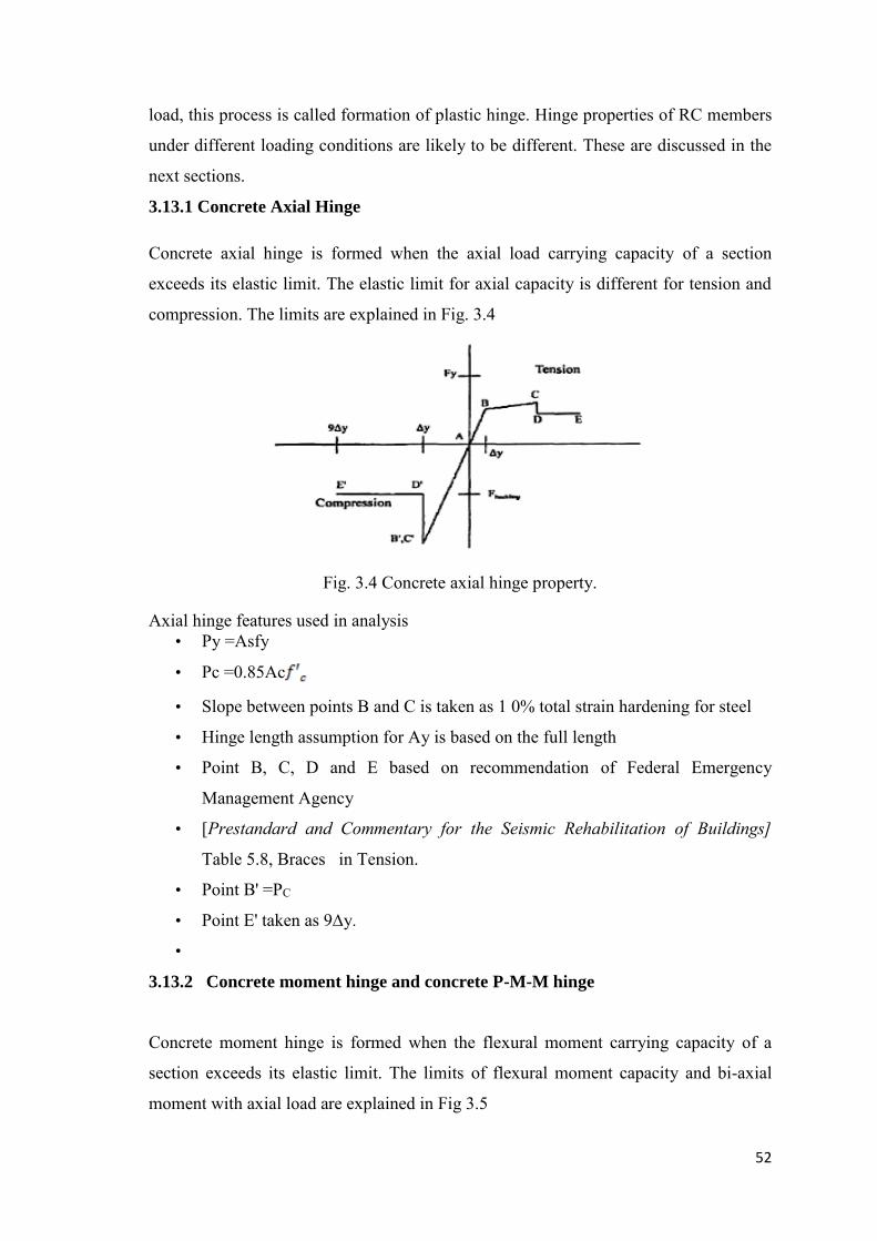
52

load, this process is called formation of plastic hinge. Hinge properties of RC members

under different loading conditions are likely to be different. These are discussed in the

next sections.

3.13.1 Concrete Axial Hinge

Concrete axial hinge is formed when the axial load carrying capacity of a section

exceeds its elastic limit. The elastic limit for axial capacity is different for tension and

compression. The limits are explained in Fig. 3.4

Fig. 3.4 Concrete axial hinge property.

Axial hinge features used in analysis • Py =Asfy

• Pc =0.85Ac

• Slope between points B and C is taken as 1 0% total strain hardening for steel

• Hinge length assumption for Ay is based on the full length

• Point B, C, D and E based on recommendation of Federal Emergency

Management Agency

• [Prestandard and Commentary for the Seismic Rehabilitation of Buildings]

Table 5.8, Braces in Tension.

• Point B' =PC

• Point E' taken as 9∆y.

•

3.13.2 Concrete moment hinge and concrete P-M-M hinge

Concrete moment hinge is formed when the flexural moment carrying capacity of a

section exceeds its elastic limit. The limits of flexural moment capacity and bi-axial

moment with axial load are explained in Fig 3.5

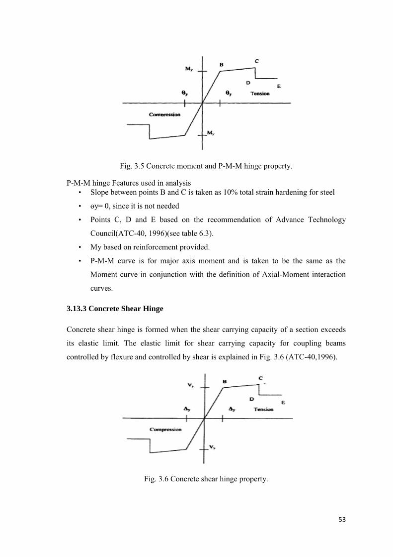
53

Fig. 3.5 Concrete moment and P-M-M hinge property.

P-M-M hinge Features used in analysis • Slope between points B and C is taken as 10% total strain hardening for steel

• ɵy= 0, since it is not needed

• Points C, D and E based on the recommendation of Advance Technology

Council(ATC-40, 1996)(see table 6.3).

• My based on reinforcement provided.

• P-M-M curve is for major axis moment and is taken to be the same as the

Moment curve in conjunction with the definition of Axial-Moment interaction

curves.

3.13.3 Concrete Shear Hinge

Concrete shear hinge is formed when the shear carrying capacity of a section exceeds

its elastic limit. The elastic limit for shear carrying capacity for coupling beams

controlled by flexure and controlled by shear is explained in Fig. 3.6 (ATC-40,1996).

Fig. 3.6 Concrete shear hinge property.

54

Shear hinge features used in analysis

• Slope between points B and C is taken as 10% total strain hardening for steel

• Vy = 2AS (fc ΄) + fyAsvd

Points C, D and E based on the recommendation of Advance Technology Council

(ATC-40, 1996).

3.14 Concrete Frame Acceptability Limits

To determine the performance of a building, response quantities from a nonlinear static

analysis are compared with limits for appropriate performance levels. Fig. 3.7

illustrates a generalized load-deformation relation applied in the structural components

under the present study. Curve Type I in the Fig. 3.7 has been used when the

deformation is a flexural plastic hinge. Curve type II in the Fig. 3.7 has been used when

the deformation is inter-storey drift, shear angle, sliding shear displacement, or beam-

column joint rotation.

Fig. 3.7 Generalized load-deformation relations for components

Tables 9-6, 9-7 and 9-12 in ATC-40 define the modeling parameters for beam and

column in terms of plastic angles within the yielding plastic hinge.

3.15 Hinge Properties for Modeling

Depending upon the longitudinal reinforcement, transverse reinforcement etc. different

hinge properties may be modeled based on the modeling parameter defined through

Tables 9-6, 9-7 and 9-12 in ATC-40. Different points A, B, C, etc. are defined in Fig.

3.3 of this Chapter. For the purpose of the thesis, the ETABS's built-in default hinge

properties of concrete have been assumed. These built-in default hinge properties are

generally based on Tables 9.6,9.7 and 9.12 in ATC-40.

55

3.16 Assumption for Pushover Analysis

The following assumptions relate to the pushover analysis of the building

• Moment (M2-M3) hinges are considered at the ends of beam members and

moment and axial. (P-M-M) is considered at the ends of column members.

Here 2 and 3 specify the axis or directions of the loads. For column members

axis 2 is perpendicular to the line object. The projection of the positive local 2

axis onto the global X-axis is in the same direction as the positive global X-axis.

Axis 3 is perpendicular to the line object. The direction of the positive local 3

axis is determined from applyingthe right-hand rule using the directions of the 1

and 2 axes where 1 is alongthe line object. For beam members, axis 2 is

perpendicular to the line object. The positive local 2 axis points in the same

direction as the global Z-axis, upward. Axis 3 is perpendicular to the line object

and is horizontal. The direction of the positive local 3 axis is determined from

applying the right-hand rule using the directions of the 1 and 2 axes where 1 is

along the line object (ETABS manual).

• Push-over analysis has been done using load pattern of equivalent static load

calculated as per provision of BNBC, 2006.

• Gravity load has been considered as the previous pushover cases for each

analysis.

• Unload entire building is selected for distribution of loads when local hinges

fail. When a hinge reaches a negative-sloped portion of the stress-strain curve,

the program continues to try to increase the applied load. If this results in

increased strain (decreased stress) the analysis proceeds. If the strain tries to

reverse, the program instead reverses the load on the whole building until the

hinge is fully unloaded to the next segment on the stress-strain curve. At this

point the program reverts to increasing the load on the building. Other parts of

the building may now pick up the load that was removed from the unloading

hinge.

• Geometric non-linearity (P-∆ effect) is considered with full dead load and 50%

live load.

• Horizontal displacement of topmost corner node has been selected for performance monitoring of the roof displacement.

56

CHAPTER 4

EFFECTS OF MASONRY INFILL IN RC BUILDINGS

4.1 Introduction

Masonry infill (MI) elements are used extensively as infill wall panels in reinforced

concrete and steel frame buildings. Masonry infill fulfill architectural and other

functional requirements, such as forming a significant portion of building envelop,

partitioning, temperature and sound barriers, while also providing adequate

compartmentalization against fire hazard. Lack of knowledge on its performance under

seismic loading has discouraged engineers from relying on the interaction of infill with

the enclosing structural system. Therefore, it has become a common practice to ignore

the participation of infill in resisting lateral loads. Research has shown the beneficial

effects of the interaction between masonry infill and structural elements for seismic

performance of existing frame buildings. Researchers have concluded that proper use of

infill in frames could result in significant increases in the strength and stiffness of

buildings subjected to seismic excitations (Klingner and Bertero 1978),(Mehrabi et al.

1996),(Bertero and Brokken 1983). However, the locations of infill in a building must

be carefully selected to avoid or minimize torsional effects as well as soft storey effect.

Architectural restrictions have to be considered when assigning these locations.

Masonry infill walls confined by reinforced concrete (RC) frames on all four sides play

a vital role in resisting the lateral seismic loads on buildings. The behavior of masonry

infilled frames has been extensively studied (Stafford Smith and Coull 1991);(Murty

and Jain 2000);(Moghaddam and Dowling 1987) in attempts to develop a rational

approach for design of such frames. It has been shown experimentally that MI walls

have a very high initial lateral stiffness and low deformability (Moghaddam and

Dowling 1987). Thus introduction of MI in RC frames changes the lateral-load transfer

mechanism of the building from predominant frame action to predominant truss action

(Murty and Jain 2000), as shown in Fig. 4.1, which is responsible for reduction in

bending moments and increase in axial forces in the frame members.

57

Fig. 4.1 Change in lateral load transfer mechanism due to masonry infill

(Murty and Jain 2000)

The high in-plane rigidity of the masonry wall significantly stiffens the otherwise

relatively flexible frame. The result is, therefore, a relatively stiff and tough bracing

system. The wall braces the frame partly by its in plane shear resistance (Fig. 4.2) and

partly by its behavior as a diagonal bracing strut.

Fig. 4.2 Analogous braced frame

The frame of Fig. 4.3 shows such mode of behavior. When the frame is subjected to

horizontal loading, it deforms with double-curvature bending of the columns and

beams. The translation of the upper part of the column in each storey and the shortening

of the leading diagonal of the frame cause the column to lean against the wall as well as

58

to compress the wall along its diagonal. It is roughly analogous to a diagonally braced

frame, shown in fig 4.3.The potential modes of failure, of the wall arise as results of its

interaction with the frame are given below

1. Tension failure of the tension column due to overturning moments.

2. Flexure or shear failure of the columns.

3. Compression failure of the diagonal strut.

4. Diagonal tension cracking of the panel and

5. Sliding shear failure of the masonry along horizontal mortar beds the above failure

modes are shown in Fig. 4.4 and 4.5.

The "perpendicular" tensile stresses are caused by the divergence of the compressive

stress trajectories on opposite sides of the leading diagonal as they approach the middle

region of the infill. The diagonal cracking is initiated at and spreads from the middle of

the infill, where the tensile stresses are a maximum, tending to stop near the

compression corners, where the tension is suppressed.

Fig. 4.3 Modes of infill failure

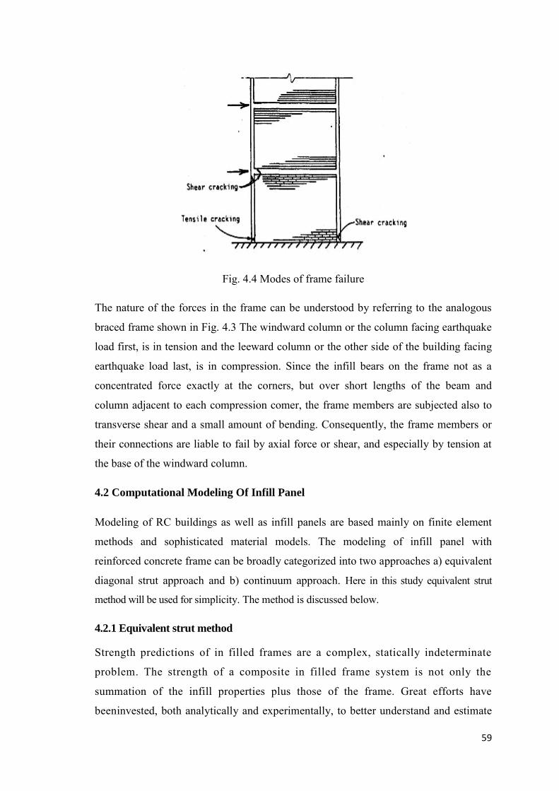
59

Fig. 4.4 Modes of frame failure

The nature of the forces in the frame can be understood by referring to the analogous

braced frame shown in Fig. 4.3 The windward column or the column facing earthquake

load first, is in tension and the leeward column or the other side of the building facing

earthquake load last, is in compression. Since the infill bears on the frame not as a

concentrated force exactly at the corners, but over short lengths of the beam and

column adjacent to each compression comer, the frame members are subjected also to

transverse shear and a small amount of bending. Consequently, the frame members or

their connections are liable to fail by axial force or shear, and especially by tension at

the base of the windward column.

4.2 Computational Modeling Of Infill Panel

Modeling of RC buildings as well as infill panels are based mainly on finite element

methods and sophisticated material models. The modeling of infill panel with

reinforced concrete frame can be broadly categorized into two approaches a) equivalent

diagonal strut approach and b) continuum approach. Here in this study equivalent strut

method will be used for simplicity. The method is discussed below.

4.2.1 Equivalent strut method

Strength predictions of in filled frames are a complex, statically indeterminate

problem. The strength of a composite in filled frame system is not only the

summation of the infill properties plus those of the frame. Great efforts have

beeninvested, both analytically and experimentally, to better understand and estimate

60

the composite behavior of masonry in filled frames, (Polyakov 1960)(work back to

the early 1950s),(Stafford Smith and Carter 1969), (Klingner and Bertero 1978), , to

mention just a few, formed the basis for understanding and predicting in filled frame

in-plane behavior. Their experimental testing of in filledframes under lateral loads

resulted in specimen deformation shapes similar to the one illustrated in Fig 4.5.

Fig. 4.5 Specimen deformation shape

During testing of the specimens, diagonal cracks developed in the center of the panel,

gaps formed between the frame and the infill in the non-loaded diagonal corners of the

specimens, while full contact was observed in the two loaded diagonal corners. This

behavior, initially observed by Polyakov, lead to the simplification in filled frame analysis

by replacing the masonry infill with an equivalent compressive masonry strut as shown in

Fig. 4.5. The equivalent masonry strut of width, a, with same net thickness and

mechanical properties (such as the modulus of elasticity, Em) as the infill itself, is assumed

to be pinned at both ends to the confining frame.

4.2.2 Equivalent strut width

The evaluation of the equivalent width, a, varies from one reference to the other.The

most simplistic approaches by (Paulay and Priestley 1992) and (Mehrabi et al. 1996)

have assumed constant values for strut width, a, between 12.5 to 25 percent of the

diagonal dimension of the infill, with no regard for any infill or frame

properties.(Stafford Smith and Carter 1969), (Mainstone 1971), and others, derived

complex expressions to estimate the equivalent strut width, a, that consider parameters like

the length of contact between the column/beam and infill, as well the relative

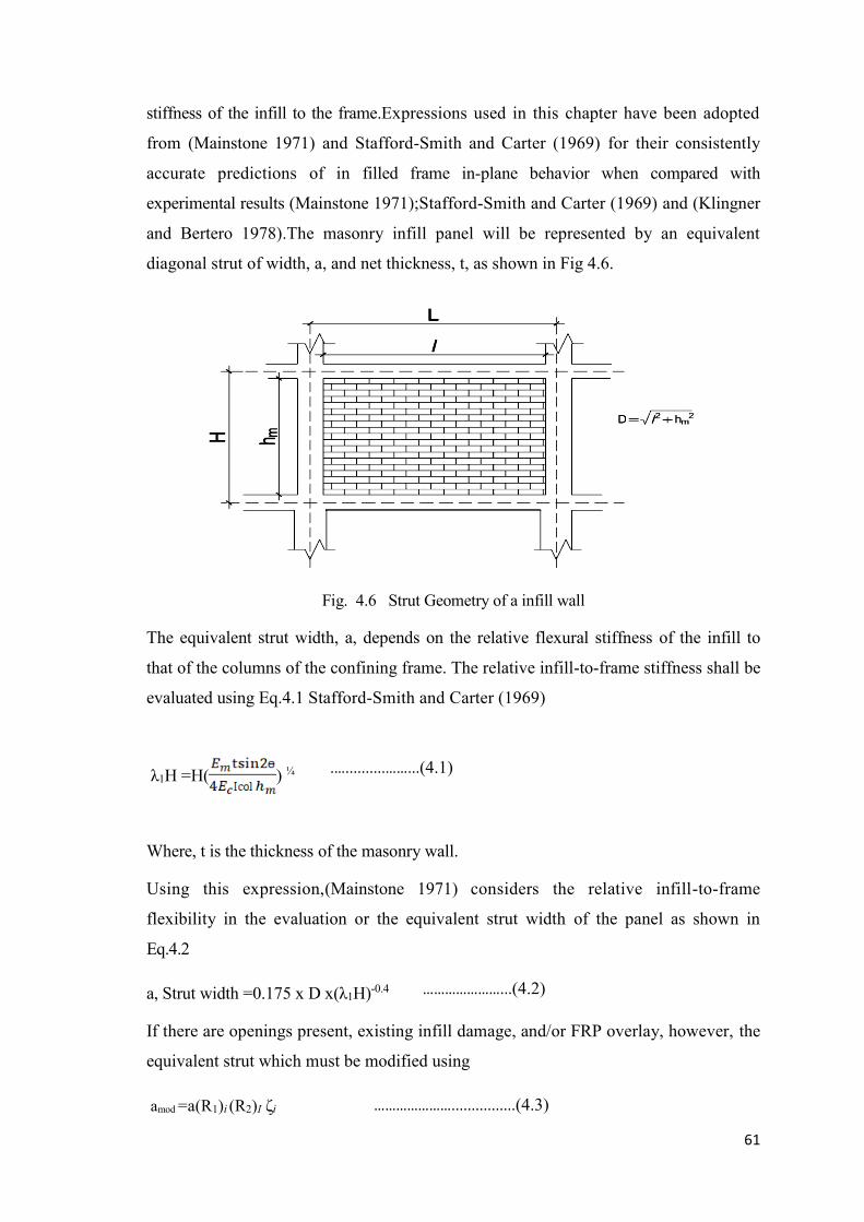
61

stiffness of the infill to the frame.Expressions used in this chapter have been adopted

from (Mainstone 1971) and Stafford-Smith and Carter (1969) for their consistently

accurate predictions of in filled frame in-plane behavior when compared with

experimental results (Mainstone 1971);Stafford-Smith and Carter (1969) and (Klingner

and Bertero 1978).The masonry infill panel will be represented by an equivalent

diagonal strut of width, a, and net thickness, t, as shown in Fig 4.6.

Fig. 4.6 Strut Geometry of a infill wall

The equivalent strut width, a, depends on the relative flexural stiffness of the infill to

that of the columns of the confining frame. The relative infill-to-frame stiffness shall be

evaluated using Eq.4.1 Stafford-Smith and Carter (1969)

λ1H =H( ) ¼

Where, t is the thickness of the masonry wall.

Using this expression,(Mainstone 1971) considers the relative infill-to-frame

flexibility in the evaluation or the equivalent strut width of the panel as shown in

Eq.4.2

a, Strut width =0.175 x D x(λ1H)-0.4

If there are openings present, existing infill damage, and/or FRP overlay, however, the

equivalent strut which must be modified using

amod =a(R1)i (R2)I ζi

.…..........……...(4.1)

…………………...(4.2)

…………………................(4.3)

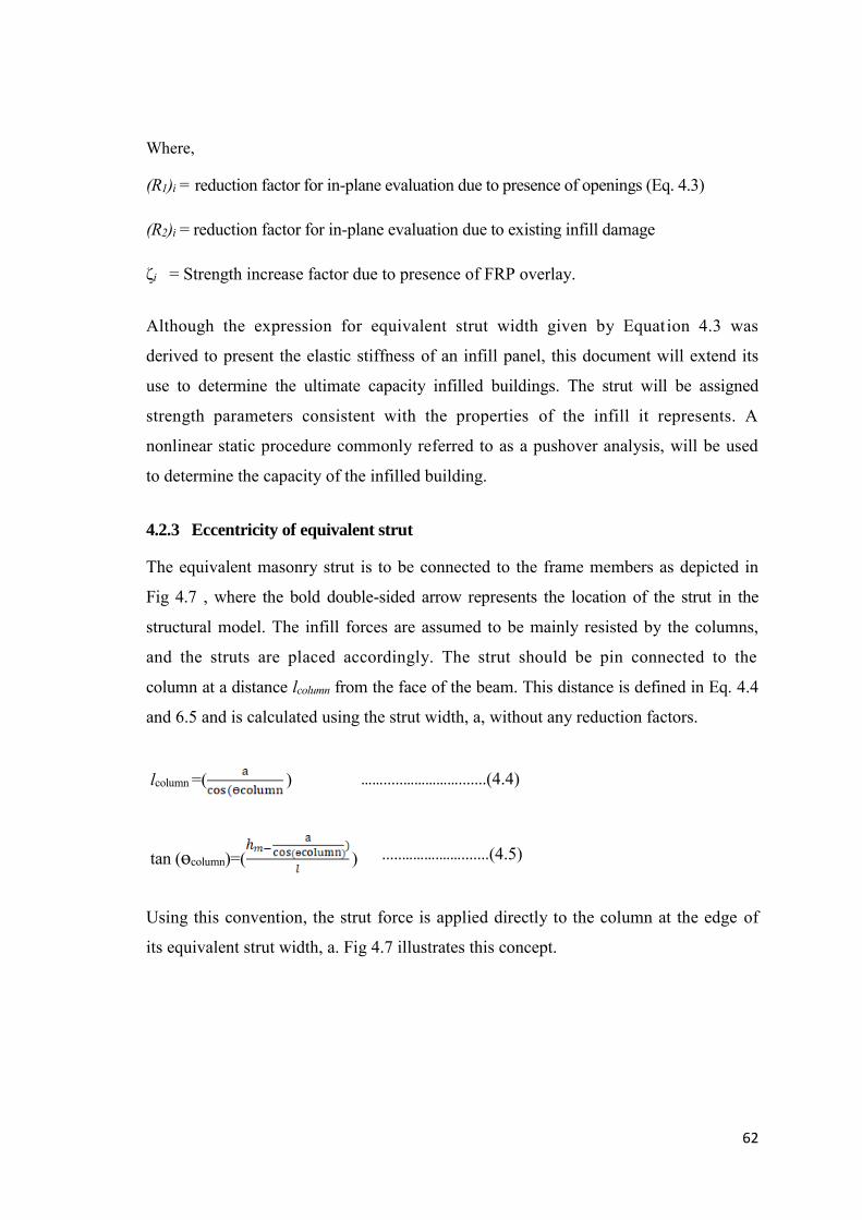
62

Where,

(R1)i = reduction factor for in-plane evaluation due to presence of openings (Eq. 4.3)

(R2)i = reduction factor for in-plane evaluation due to existing infill damage

ζi = Strength increase factor due to presence of FRP overlay.

Although the expression for equivalent strut width given by Equation 4.3 was

derived to present the elastic stiffness of an infill panel, this document will extend its

use to determine the ultimate capacity infilled buildings. The strut will be assigned

strength parameters consistent with the properties of the infill it represents. A

nonlinear static procedure commonly referred to as a pushover analysis, will be used

to determine the capacity of the infilled building.

4.2.3 Eccentricity of equivalent strut

The equivalent masonry strut is to be connected to the frame members as depicted in

Fig 4.7 , where the bold double-sided arrow represents the location of the strut in the

structural model. The infill forces are assumed to be mainly resisted by the columns,

and the struts are placed accordingly. The strut should be pin connected to the

column at a distance lcolumn from the face of the beam. This distance is defined in Eq. 4.4

and 6.5 and is calculated using the strut width, a, without any reduction factors.

lcolumn =( )

tan (ɵcolumn)=( )

Using this convention, the strut force is applied directly to the column at the edge of

its equivalent strut width, a. Fig 4.7 illustrates this concept.

…….....…………….......(4.4)

.....……….…….......(4.5)

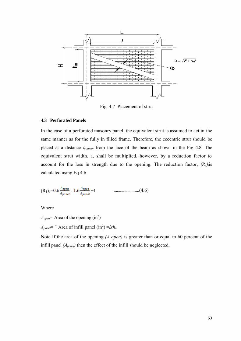
63

Fig. 4.7 Placement of strut

4.3 Perforated Panels

In the case of a perforated masonry panel, the equivalent strut is assumed to act in the

same manner as for the fully in filled frame. Therefore, the eccentric strut should be

placed at a distance lcolumn from the face of the beam as shown in the Fig 4.8. The

equivalent strut width, a, shall be multiplied, however, by a reduction factor to

account for the loss in strength due to the opening. The reduction factor, (R1)iis

calculated using Eq.4.6

(R1)i = - +1

Where

Aopen= Area of the opening (in2)

Apanel= = Area of infill panel (in2) =lxhm

Note If the area of the opening (A open) is greater than or equal to 60 percent of the

infill panel (Apanel) then the effect of the infill should be neglected.

.....…………….....(4.6)

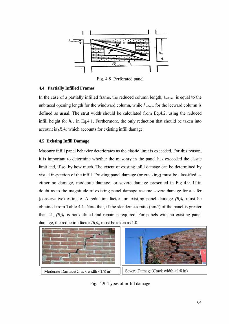
64

Fig. 4.8 Perforated panel

4.4 Partially Infilled Frames

In the case of a partially infilled frame, the reduced column length, lcolumn is equal to the

unbraced opening length for the windward column, while lcolumn for the leeward column is

defined as usual. The strut width should be calculated from Eq.4.2, using the reduced

infill height for hm, in Eq.4.1. Furthermore, the only reduction that should be taken into

account is (R2)i; which accounts for existing infill damage.

4.5 Existing Infill Damage

Masonry infill panel behavior deteriorates as the elastic limit is exceeded. For this reason,

it is important to determine whether the masonry in the panel has exceeded the elastic

limit and, if so, by how much. The extent of existing infill damage can be determined by

visual inspection of the infill. Existing panel damage (or cracking) must be classified as

either no damage, moderate damage, or severe damage presented in Fig 4.9. If in

doubt as to the magnitude of existing panel damage assume severe damage for a safer

(conservative) estimate. A reduction factor for existing panel damage (R2)i, must be

obtained from Table 4.1. Note that, if the slenderness ratio (hm/t) of the panel is greater

than 21, (R2)i, is not defined and repair is required. For panels with no existing panel

damage, the reduction factor (R2)i; must be taken as 1.0.

Fig. 4.9 Types of in-fill damage

Moderate Damage(Crack width <1/8 in) Severe Damage(Crack width >1/8 in)

65

Table 4.1 In-plane damage reduction factor

(R2)i, for Type of Damage

hm/t Moderate Severe

<21 0.7 0.4

>21 Requires repair.

4.6 Properties to be Determined

The infill masonry panel will be represented as strut member. The equivalent strut

width shall be determined according to Coull and Smith described earlier. For the

modeling of infill the following properties must be determined.

Modulus of elasticity of concrete Ec value for column and beam materials.

Sectional properties (i.e. Depth, Width, Moment of Inertia, centroid) of the

column and beam.

Equivalent width of the masonry infill strut "a"

fm, compressive strength of the masonry assemble units.

Em modulus of elasticity of the masonry unit.

4.7 Calculation of Equivalent Strut Width

Detail sample calculation of equivalent strut width and eccentricity is given in the

appendix C.

66

CHAPTER 5

SEISMIC PERFORMANCE EVALUATION OF TWO 06 (SIX) STOREY RC

BUILDINGS

5.1 General

For the performance evaluation purposes Dhaka is selected as the site and seismic

demand for Dhaka has been estimated as per guideline of ATC-40.Structural

performances of an existing 6(Six) storey building of medium-rise building of height

around 60 feet have been ivestigated.This height range has been selected because of the

fact that buildings with this height range are very common in Dhaka city. The

performances of the buildings as evaluated through pushover analysis have been

presented through capacity curves and capacity spectrums described in the sections that

follow.

5.2 Structural Characteristic Features of Building 1

Building 1 considered in this study is located at Mohakhali.

For basic design and evaluation of the buildings the following loading conditions have

been considered. Self-weight of the building has been assumed as per geometric

dimension of the structural elements with the unit weight of the concrete has been taken

as 150 lb/ft3. Other loading due to partition wall, floor finish, cladding loading etc are

considered as per available drawing of the selected building. Code specified floor finish

30 lb/ft2 has been considered on the floors and live load considered as 40 lb/ft2

irrespective of different use/inhabitable area. Seismic load has been considered as per

UBC 1994 loading and base shear has been compared with BNBC 2006. Equivalent

Static Load method has been used with response modification factor, R = 8. No live

load has been considered in calculating Seismic Dead Load. Other coefficients used in

seismic load calculation are Z =0.15, I = 1.0, S = 1.5. Earthquake load at any level

equally distributed among all the nodes in that level.

The material properties and relevant features are as follows

The building was designed with load combination defined in the ETABS 9.7.4 with

• Cylinder strength of concrete, f”c = 3000 psi (as per drawing)

• Yield strength of steel fy= 60000 psi (as per drawing)

67

Sections of the columns and beams as per drawing have been chosen.

• Column sizes are 10"x20",10"x24",10"x32",10"x36"

• Beam sizes are 10"x20.5"

• Grade Beam sizes are 12"x18"

• Slab Thickness is 5.5"

• Shear Wall Thickness is 6"

• All supports are considered as fixed support.

The following assumptions are considered for the pushover analysis of the building

• Moment (M3) hinges are considered at the ends of beam members and P-M-M

hinges are considered at the ends of the column members. All hinges are according

to as per ATC 40 document.

• Pushover analysis has been done using load pattern Equivalent Static Load of

BNBC 2006. Load intensities have been normalized with the base shear.

Geometric non-linearity (P-∆ effect) of the building was considered with full dead

loads and 50% of the live load.

• In each case, the horizontal displacement of the right top most node of the building

has been selected for performance monitoring of roof displacement.

• The general-purpose finite element program ETABS-9.7.4. has been used as the

tool for modeling the buildings and study its behavior in terms of capacity and

performance. Non-linear Static Pushover analysis has also been done using the same

program.

5.3 Performance Evaluation of The Building 1

The buildingis modeled and analyzed using Etabs-9.7.4. After analyzing the buildings,

hinges defined in ATC-40,1996 have been assigned to the respective members and

pushover analyses have been performed to develop capacity curves for each of the

buildings. The capacity curves such as base shear - displacement and capacity

spectrums can be obtained after push over analysis. Accordingly performance points of

the buildings for the estimated seismic demand have been determined from the curve.

Resulting outputs for building presented next. Hinge states near the performance point

have been shown in color code. Different performance levels are determined as per

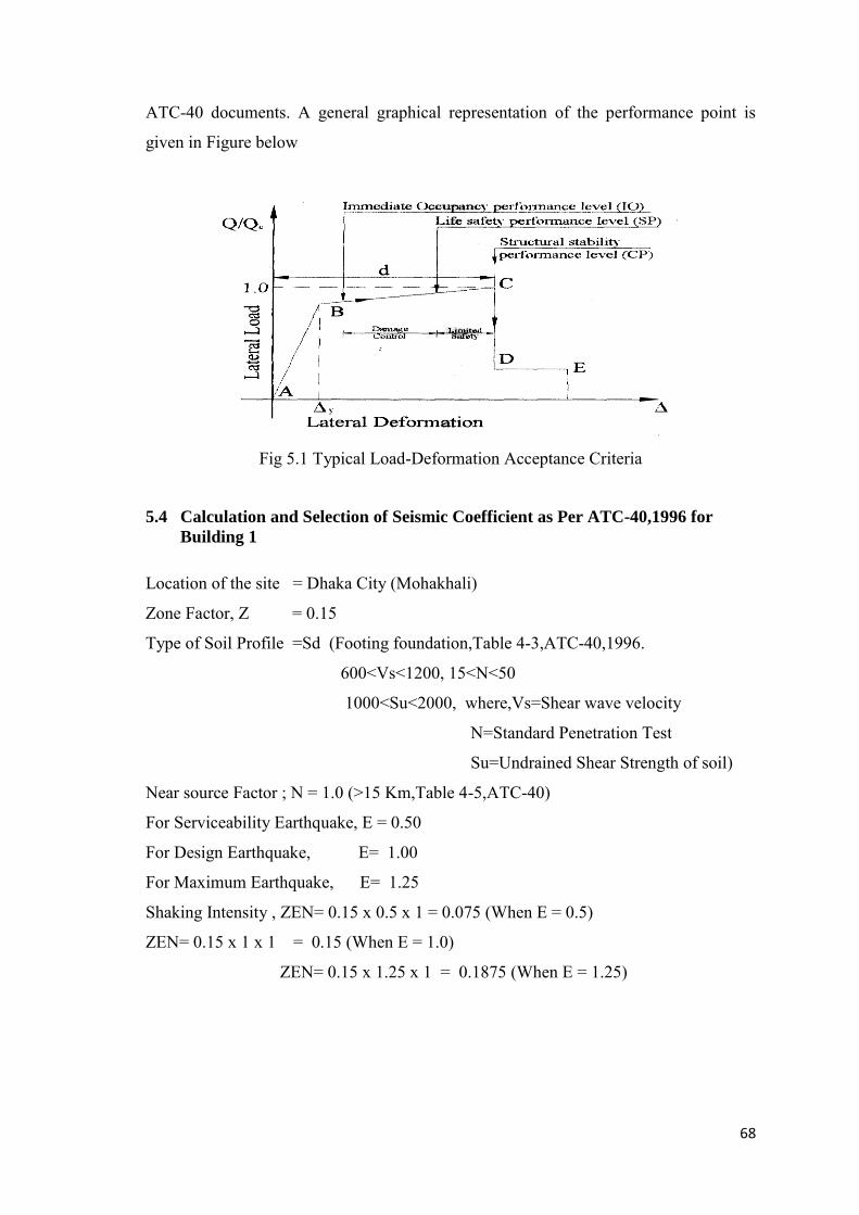
68

ATC-40 documents. A general graphical representation of the performance point is

given in Figure below

Fig 5.1 Typical Load-Deformation Acceptance Criteria

5.4 Calculation and Selection of Seismic Coefficient as Per ATC-40,1996 for

Building 1 Location of the site = Dhaka City (Mohakhali)

Zone Factor, Z = 0.15

Type of Soil Profile =Sd (Footing foundation,Table 4-3,ATC-40,1996.

600<Vs<1200, 15<N<50

1000<Su<2000, where,Vs=Shear wave velocity

N=Standard Penetration Test

Su=Undrained Shear Strength of soil)

Near source Factor ; N = 1.0 (>15 Km,Table 4-5,ATC-40)

For Serviceability Earthquake, E = 0.50

For Design Earthquake, E= 1.00

For Maximum Earthquake, E= 1.25

Shaking Intensity , ZEN= 0.15 x 0.5 x 1 = 0.075 (When E = 0.5)

ZEN= 0.15 x 1 x 1 = 0.15 (When E = 1.0)

ZEN= 0.15 x 1.25 x 1 = 0.1875 (When E = 1.25)

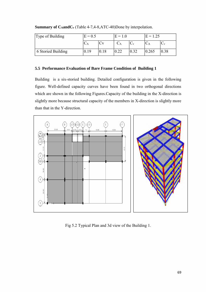
69

Summary of CAandCv (Table 4-7,4-8,ATC-40)Done by interpolation.

Type of Building E = 0.5 E = 1.0 E = 1.25 CA Cv CA Cv CA Cv

6 Storied Building 0.19 0.18 0.22 0.32 0.265 0.38

5.5 Performance Evaluation of Bare Frame Condition of Building 1

Building is a six-storied building. Detailed configuration is given in the following

figure. Well-defined capacity curves have been found in two orthogonal directions

which are shown in the following Figures.Capacity of the building in the X-direction is

slightly more because structural capacity of the members in X-direction is slightly more

than that in the Y-direction.

Fig 5.2 Typical Plan and 3d view of the Building 1.

70

The Capacity curves have been converted into capacity spectrums as per pushover

analysis using ETABS-9.7.4, which are shown in following Figures below.

Fig 5.3 Base shear vs Displacement curve in X Direction for bare frame condition of building 1 at maximum EQ .

Fig 5.4 Base shear vs Displacement curve in Y Direction for bare frame condition of building 1 at maximum EQ .

71

Fig 5.5 Capacity spectrum curve in X Direction for bare frame condition of building 1 at maximum EQ.

Fig 5.6 Capacity spectrum curve in Y Direction for for condition of building 1 at Maximum EQ.

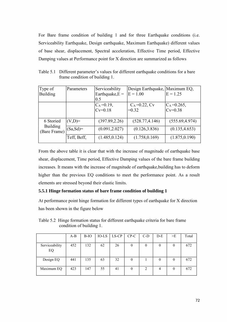
72

For Bare frame condition of building 1 and for three Earthquake conditions (i.e.

Serviceability Earthquake, Design earthquake, Maximum Earthquake) different values

of base shear, displacement, Spectral acceleration, Effective Time period, Effective

Damping values at Performance point for X direction are summarized as follows

Table 5.1 Different parameter’s values for different earthquake conditions for a bare frame condition of building 1. Type of Building

Parameters Serviceability Earthquake,E = 0.5

Design Earthquake, E = 1.00

Maximum EQ, E = 1.25

CA =0.19, Cv=0.18

CA =0.22, Cv =0.32

CA =0.265, Cv=0.38

6 Storied Building

(Bare Frame)

(V,D)= (397.89,2.26) (528.77,4.146) (555.69,4.974)

(Sa,Sd)= (0.091,2.027) (0.126,3.836) (0.135,4.653)

Teff, Beff, (1.485,0.124) (1.758,0.169) (1.875,0.190)

From the above table it is clear that with the increase of magnitude of earthquake base

shear, displacement, Time period, Effective Damping values of the bare frame building

increases. It means with the increase of magnitude of earthquake,building has to deform

higher than the previous EQ conditions to meet the performance point. As a result

elements are stressed beyond their elastic limits.

5.5.1 Hinge formation status of bare frame condition of building 1

At performance point hinge formation for different types of earthquake for X direction

has been shown in the figure below

Table 5.2 Hinge formation status for different earthquake criteria for bare frame condition of building 1.

A-B B-IO IO-LS LS-CP CP-C C-D D-E >E Total

Serviceability EQ

452 132 62 26 0 0 0 0 672

Design EQ 441 135 63 32 0 1 0 0 672

Maximum EQ 423 147 55 41 0 2 4 0 672

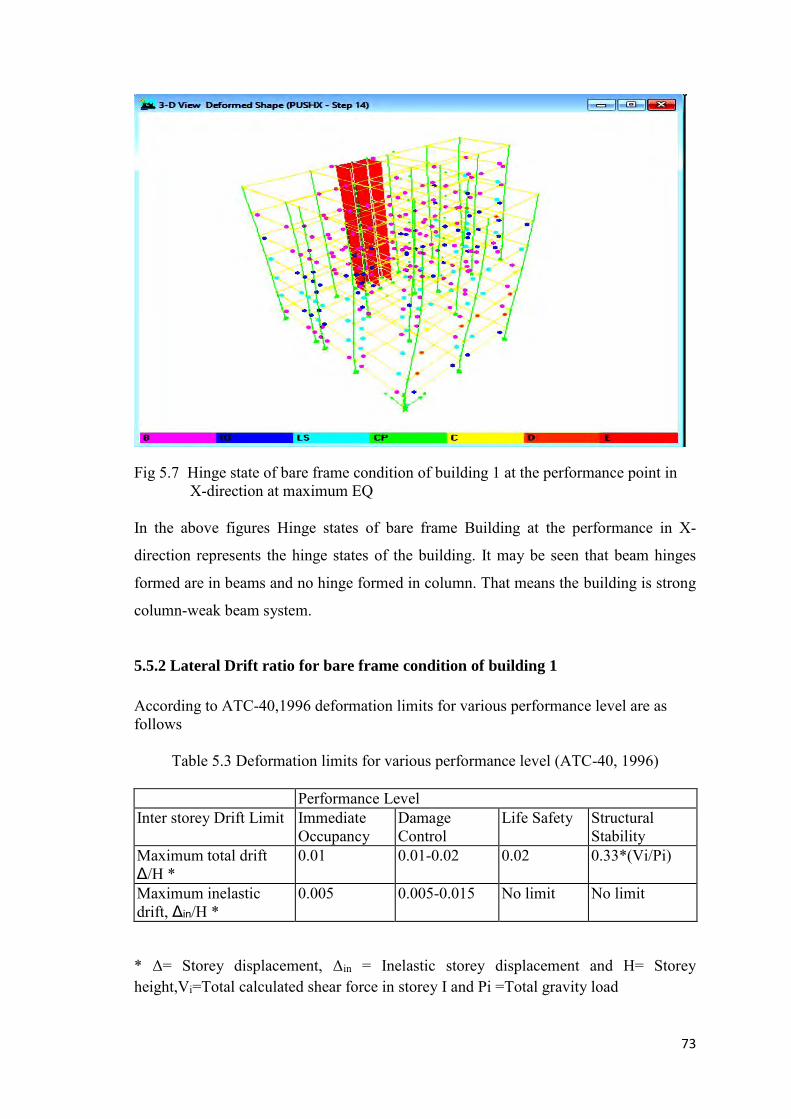
73

Fig 5.7 Hinge state of bare frame condition of building 1 at the performance point in X-direction at maximum EQ In the above figures Hinge states of bare frame Building at the performance in X-

direction represents the hinge states of the building. It may be seen that beam hinges

formed are in beams and no hinge formed in column. That means the building is strong

column-weak beam system.

5.5.2 Lateral Drift ratio for bare frame condition of building 1

According to ATC-40,1996 deformation limits for various performance level are as follows

Table 5.3 Deformation limits for various performance level (ATC-40, 1996) Performance Level Inter storey Drift Limit Immediate

Occupancy Damage Control

Life Safety Structural Stability

Maximum total drift Δ/H *

0.01 0.01-0.02 0.02 0.33*(Vi/Pi)

Maximum inelastic drift, Δin/H *

0.005 0.005-0.015 No limit No limit

* Δ= Storey displacement, Δin = Inelastic storey displacement and H= Storey height,Vi=Total calculated shear force in storey I and Pi =Total gravity load

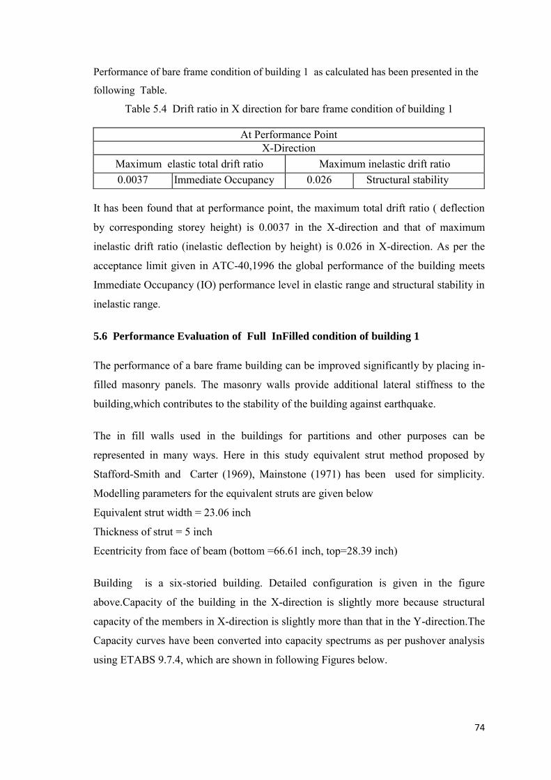
74

Performance of bare frame condition of building 1 as calculated has been presented in the

following Table.

Table 5.4 Drift ratio in X direction for bare frame condition of building 1

At Performance Point X-Direction

Maximum elastic total drift ratio Maximum inelastic drift ratio 0.0037 Immediate Occupancy 0.026 Structural stability

It has been found that at performance point, the maximum total drift ratio ( deflection

by corresponding storey height) is 0.0037 in the X-direction and that of maximum

inelastic drift ratio (inelastic deflection by height) is 0.026 in X-direction. As per the

acceptance limit given in ATC-40,1996 the global performance of the building meets

Immediate Occupancy (IO) performance level in elastic range and structural stability in

inelastic range.

5.6 Performance Evaluation of Full InFilled condition of building 1

The performance of a bare frame building can be improved significantly by placing in-

filled masonry panels. The masonry walls provide additional lateral stiffness to the

building,which contributes to the stability of the building against earthquake.

The in fill walls used in the buildings for partitions and other purposes can be

represented in many ways. Here in this study equivalent strut method proposed by

Stafford-Smith and Carter (1969), Mainstone (1971) has been used for simplicity.

Modelling parameters for the equivalent struts are given below

Equivalent strut width = 23.06 inch

Thickness of strut = 5 inch

Ecentricity from face of beam (bottom =66.61 inch, top=28.39 inch)

Building is a six-storied building. Detailed configuration is given in the figure

above.Capacity of the building in the X-direction is slightly more because structural

capacity of the members in X-direction is slightly more than that in the Y-direction.The

Capacity curves have been converted into capacity spectrums as per pushover analysis

using ETABS 9.7.4, which are shown in following Figures below.

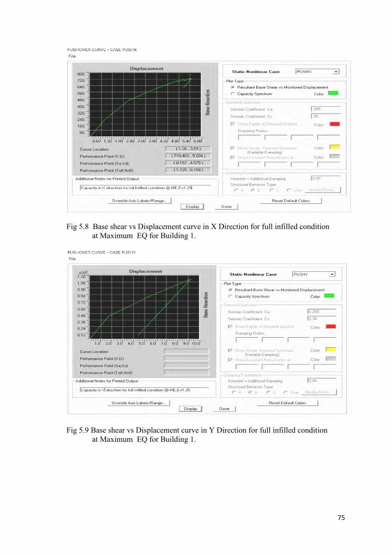
75

Fig 5.8 Base shear vs Displacement curve in X Direction for full infilled condition at Maximum EQ for Building 1.

Fig 5.9 Base shear vs Displacement curve in Y Direction for full infilled condition at Maximum EQ for Building 1.

76

Fig 5.10 Capacity Spectrum curve in X Direction for ful infilled condition at Maximum EQ Condition for Building 1.

Fig 5.11 Capacity Spectrum curve in Y Direction for ful infilled condition at Maximum EQ for Building 1.

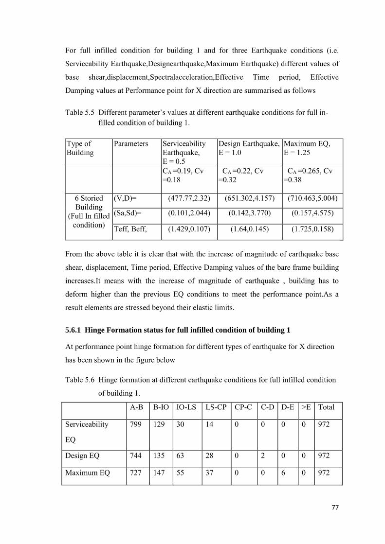
77

For full infilled condition for building 1 and for three Earthquake conditions (i.e.

Serviceability Earthquake,Designearthquake,Maximum Earthquake) different values of

base shear,displacement,Spectralacceleration,Effective Time period, Effective

Damping values at Performance point for X direction are summarised as follows

Table 5.5 Different parameter’s values at different earthquake conditions for full infilled condition of building 1. Type of Building

Parameters Serviceability Earthquake, E = 0.5



CA =0.19, Cv =0.18

CA =0.22, Cv =0.32

CA =0.265, Cv =0.38

6 Storied Building

(Full In filled condition)

(V,D)= (477.77,2.32) (651.302,4.157) (710.463,5.004)

(Sa,Sd)= (0.101,2.044) (0.142,3.770) (0.157,4.575)

Teff, Beff, (1.429,0.107) (1.64,0.145) (1.725,0.158)



increases.It means with the increase of magnitude of earthquake , building has to

deform higher than the previous EQ conditions to meet the performance point.As a

result elements are stressed beyond their elastic limits.

5.6.1 Hinge Formation status for full infilled condition of building 1



Table 5.6 Hinge formation at different earthquake conditions for full infilled condition

of building 1.


Serviceability

EQ

799 129 30 14 0 0 0 0 972

Design EQ 744 135 63 28 0 2 0 0 972

Maximum EQ 727 147 55 37 0 0 6 0 972

78

Fig 5.12 Hinge state of full infilled condition of building 1 at the performance point in X- Direction at Maximum EQ. In the above figures Hinge states of bare frame Building at the performance in X-

direction represents the hinge states of the building It may be seen that beam hinges

formed are in beams and no hinge formed in column. That means the building is strong

column-weak beam system.

5.6.2 Lateral drift ratio for full infilled condition of building 1

Performance of full infilled frame building as calculated has been presented in the following Table.

Table 5.7 Drift ratio in X direction for a full in-filled condition of building 1

At Performance Point X-Direction

Maximum total drift rati0 Maximum inelastic drift ratio

0.0036 Immediate Occupancy 0.025 Structural stability

It has been found that at performance point, the maximum total drift ratio (total

deflection by total height) is 0.0036 in the X-direction and that of maximum inelastic

drift ratio (inelastic deflection by total height) is 0.025 in X-direction. As per the

79


Immediate Occupancy (IO) performance level in elastic range and structural stability in

inelastic range.

5.7 Performance Evaluation of Soft Storey Condition of Building 1

Building is a six-storied building. Detailed configuration is given in the figure above.

Formation of a soft storey is caused by the difference in storey stiffness with the upper

stories.The stiffness difference in between stories is mainly caused by having bare

ground floor while the upper floor have in filled masonry panel. This is most common

case in residential building and could be fatal in earthquake.A regular 6 storey building

which has all the storey height same was designed first and then to use the ground floor

as a car parking, its partition walls were removed,which has become a soft storey.

Loading condition, material property and salient features of the building are same as the

full- infilled condition of building described as before.

Detailed configuration is given in the figure above.Capacity of the building in the X-

direction is slightly more because structural capacity of the members in X-direction is

slightly more than that in the Y-direction.


analysis using Etabs-v-9.7.4, which are shown in following Figures below.

Fig 5.13 Base shear vs Displacement curve in X Direction for soft storey condition at Maximum EQ for Building 1.

80

Fig 5.14 Base shear vs Displacement curve in Y Direction for soft storey condition at Maximum EQ for Building 1.

Fig 5.15 Capacity Spectrum curve in X Direction for soft storey condition at Maximum EQ for Building 1.

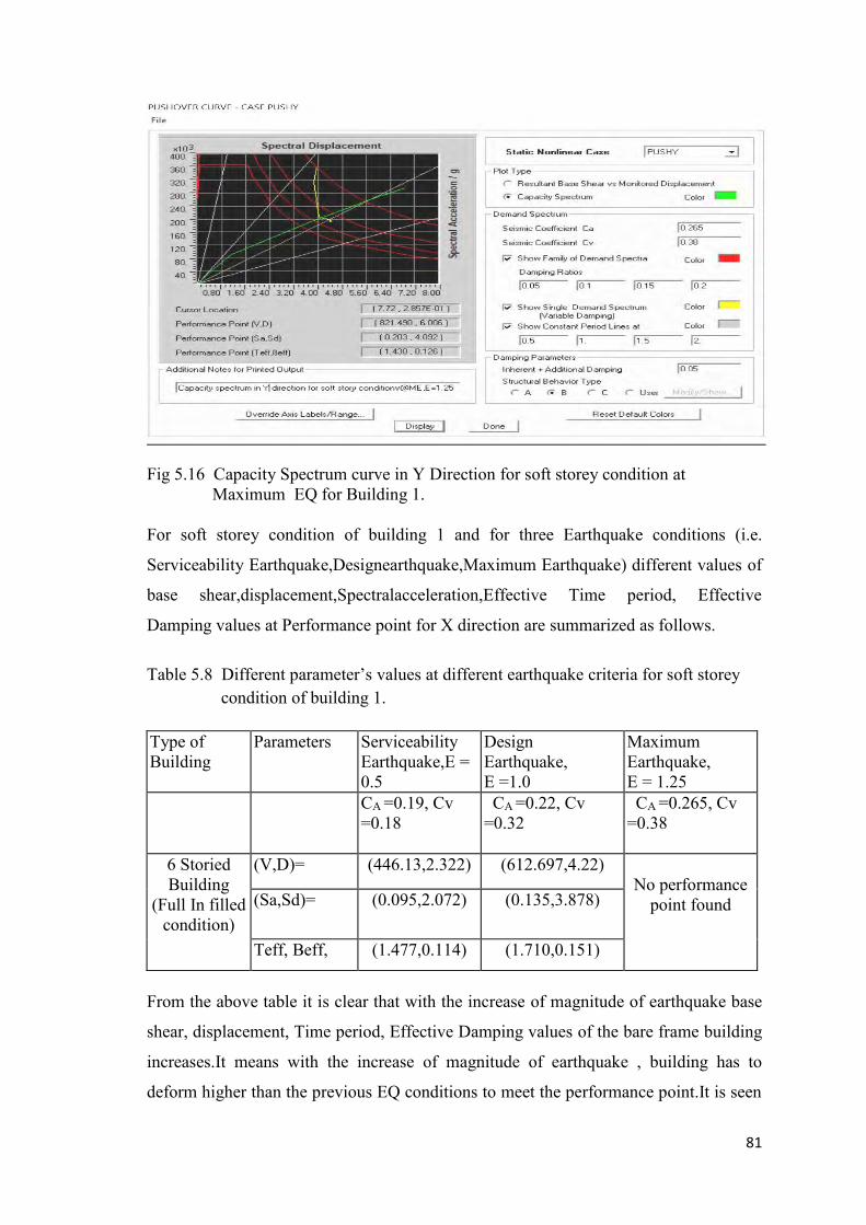
81

Fig 5.16 Capacity Spectrum curve in Y Direction for soft storey condition at Maximum EQ for Building 1. For soft storey condition of building 1 and for three Earthquake conditions (i.e.



Damping values at Performance point for X direction are summarized as follows.

Table 5.8 Different parameter’s values at different earthquake criteria for soft storey condition of building 1. Type of Building


Design Earthquake, E =1.0

Maximum Earthquake, E = 1.25

CA =0.19, Cv =0.18

CA =0.22, Cv =0.32

CA =0.265, Cv =0.38

6 Storied Building

(Full In filled condition)

(V,D)= (446.13,2.322) (612.697,4.22) No performance

point found (Sa,Sd)= (0.095,2.072) (0.135,3.878)

Teff, Beff, (1.477,0.114) (1.710,0.151)




deform higher than the previous EQ conditions to meet the performance point.It is seen

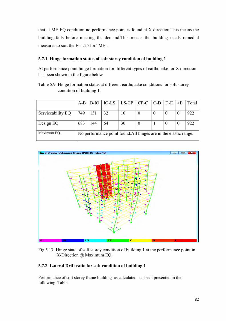
82

that at ME EQ condition no performance point is found at X direction.This means the

building fails before meeting the demand.This means the building needs remedial

measures to suit the E=1.25 for “ME”.

5.7.1 Hinge formation status of soft storey condition of building 1

At performance point hinge formation for different types of earthquake for X direction has been shown in the figure below

Table 5.9 Hinge formation status at different earthquake conditions for soft storey condition of building 1. A-B B-IO IO-LS LS-CP CP-C C-D D-E >E Total

Serviceability EQ 749 131 32 10 0 0 0 0 922

Design EQ 683 144 64 30 0 1 0 0 922

Maximum EQ No performance point found.All hinges are in the elastic range.

Fig 5.17 Hinge state of soft storey condition of building 1 at the performance point in X-Direction @ Maximum EQ. 5.7.2 Lateral Drift ratio for soft condition of building 1

Performance of soft storey frame building as calculated has been presented in the following Table.

83

Table 5.10 Drift ratio in X direction for soft storey condition of building 1

X-Direction Maximum total drift rati0 Maximum inelastic drift ratio

0.0038 Immediate Occupancy

0.026 Structural stability

5.8 Comparison of The Performance Evaluation of The Building 1 Considered

For Analysis

Comparison of the performance evaluation of the building 1 is shown in the table below. Table 5.11 Comparison of Different parameter’s values at different earthquake conditions for bare frame, full in-filled frame building, soft storey condition of building 1. Type of Building

Parameters

Serviceability Earthquake, E = 0.5


Maximum Earthquake, E=1.25

CA =0.19, Cv =0.18

CA =0.22, Cv =0.32

CA =0.265, Cv =0.38

6 Storied Building

(Bare Frame)

(V,D)= (397.89,2.26) (528.77,4.146) (555.69,4.974) (Sa,Sd)= (0.091,2.027) (0.126,3.836) (0.135,4.653) Teff, Beff, (1.485,0.124) (1.758,0.169) (1.875,0.190)

6 Storied Building

(Full in filled condition)

(V,D)= (477.77,2.32) (651.302,4.157) (710.463,5.004) (Sa,Sd)= (0.101,2.044) (0.142,3.770) (0.157,4.575) Teff, Beff, (1.429,0.107) (1.64,0.145) (1.725,0.158)

6 Storied Building

(Soft storey condition)


point found. (Sa,Sd)= (0.095,2.072) (0.135,3.878)

Teff, Beff, (1.477,0.114) (1.710,0.151)

5.8.1 Comparison of hinge formation and base shear of building 1

Base shear at performance point and number of hinges developed up to Performance Point for X direction at Design EQ

84

Table 5.12 Comparison of Hinge formation and base shear at design earthquake condition for bare frame, full infilled,soft storey condition of building 1

In-fill Condition of Frame

Base Shear inKN

Status of Hinge Formation at different Performance Stages

A-B B-IO 10-LS LS-CP CP-C C-D D-E >E Total

Bare Frame 529 441 135 63 32 0 1 0 0 672

Full In-filled Frame

651 744 135 63 28 0 2 0 0 972

Soft Storey Frame 613 683 144 64 30 0 1 0 0 922

Base shear at performance point and number of hinges developed up to Performance Point for X direction Maximum EQ

Table 5.13 Comparison of Hinge formation and base shear at maximum earthquake condition for bare frame, full infilled, soft storey condition of building 1


Base Shear inKN



Bare Frame 556 423 147 55 41 0 2 4 0 672


710 147 55 37 0 0 6 0 972 727

Soft Storey Frame No performance point found.

5.9 Structural Characteristic Features of Building 2

Building 1 considered in this study is located at Mirpur.

For basic design and evaluation of the buildings the following loading conditions have

been considered.Self-weight of the building has been assumed as per geometric

dimension of the structural elements with the unit weight of the concrete has been taken

as 150 lb/ft3. Other loading due to partition wall, floor finish, cladding loading etc are

considered as per available drawing of the selected building. Code specified floor finish

30 lb/ft2 has been considered on the floors and live load considered as 40 lb/ft2

irrespective of different use/inhabitable area. Seismic load has been considered as per

UBC 1994 loading and base shear has been compared with BNBC 2006. Equivalent

Static Load method has been used with response modification factor, R = 8. No live

load has been considered in calculating Seismic Dead Load. Other coefficients used in

85

seismic load calculation are Z =0.15, I = 1.0, S = 1.5. Earthquake load at any level

equally distributed among all the nodes in that level.

The material properties and relevant features are as follows.

The building was designed with load combination defined in the ETABS 9.7.4 with

• Cylinder strength of concrete, f”c = 3000 psi (as per drawing)

• Yield strength of steel fy= 60000 psi (as per drawing)

Sections of the columns and beams as per drawing have been chosen.

• Column sizes are 12"x15",

• Beam sizes are 10"x15"

• Grade Beam sizes are 12"x15"

• Slab Thickness is 5.0"

• All supports are considered as fixed support.

The assumptions for the pushover analysis are discussed above.

5.10 Performance Evaluation of The Building 2

The building is modeled and analyzed using Etabs-9.7.4. After analyzing the buildings,

hinges defined in ATC-40 have been assigned to the respective members and pushover

analyses have been performed to develop capacity curves for each of the buildings. The

capacity curves such as base shear - displacement and capacity spectrums can be

obtained after push over analysis. Accordingly performance points of the buildings for

the estimated seismic demand have been determined from the curve. Resulting outputs

for building presented next. Hinge states near the performance point have been shown

in color code. Different performance levels are determined as per ATC-40 documents.

5.11 Calculation and Selection of Seismic Coefficient as Per ATC-40,1996 for

building 2 Location of the site = Dhaka City (Mirpur)

Zone Factor, Z = 0.15

Type of Soil Profile =Sd (Footing foundation,Table 4-3,ATC-40,1996

600<Vs<1200, 15<N<50

1000<Su<2000, where,Vs=Shear wave velocity

N=Standard Penetration Test

Su=Undrained Shear Strength of soil)

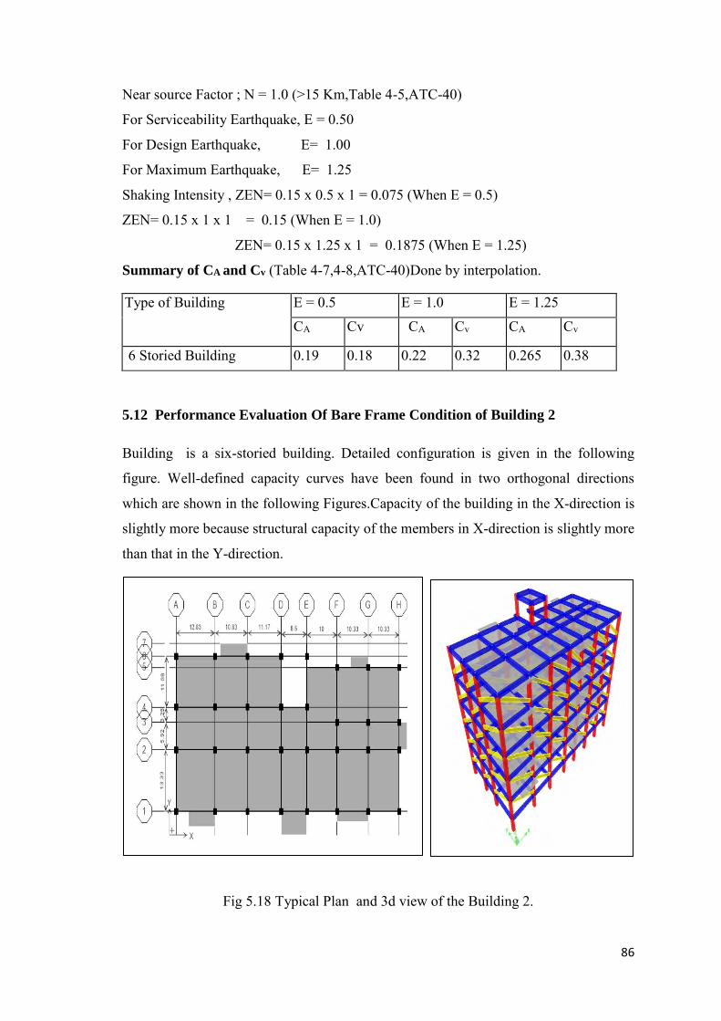
86

Near source Factor ; N = 1.0 (>15 Km,Table 4-5,ATC-40)

For Serviceability Earthquake, E = 0.50

For Design Earthquake, E= 1.00

For Maximum Earthquake, E= 1.25

Shaking Intensity , ZEN= 0.15 x 0.5 x 1 = 0.075 (When E = 0.5)

ZEN= 0.15 x 1 x 1 = 0.15 (When E = 1.0)

ZEN= 0.15 x 1.25 x 1 = 0.1875 (When E = 1.25)

Summary of CA and Cv (Table 4-7,4-8,ATC-40)Done by interpolation.

Type of Building E = 0.5 E = 1.0 E = 1.25 CA Cv CA Cv CA Cv

6 Storied Building 0.19 0.18 0.22 0.32 0.265 0.38

5.12 Performance Evaluation Of Bare Frame Condition of Building 2

Building is a six-storied building. Detailed configuration is given in the following

figure. Well-defined capacity curves have been found in two orthogonal directions

which are shown in the following Figures.Capacity of the building in the X-direction is

slightly more because structural capacity of the members in X-direction is slightly more

than that in the Y-direction.

Fig 5.18 Typical Plan and 3d view of the Building 2.

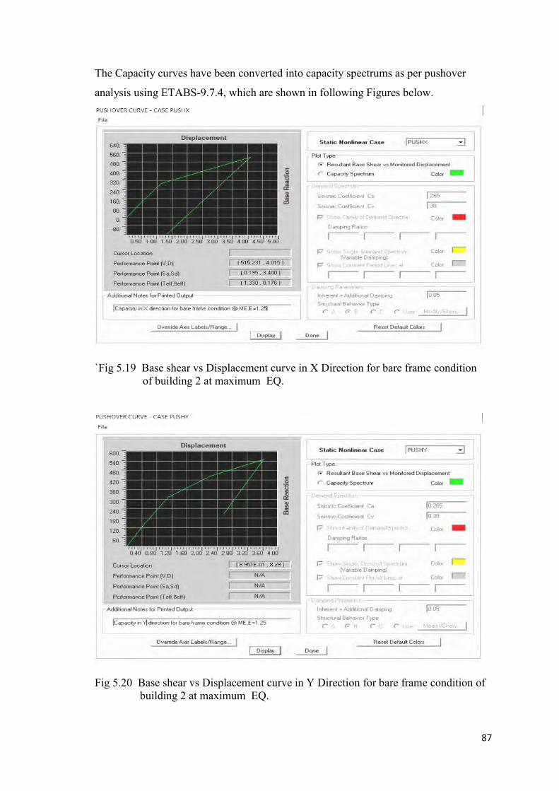
87


analysis using ETABS-9.7.4, which are shown in following Figures below.

`Fig 5.19 Base shear vs Displacement curve in X Direction for bare frame condition of building 2 at maximum EQ.

Fig 5.20 Base shear vs Displacement curve in Y Direction for bare frame condition of building 2 at maximum EQ.

88

Fig 5.21 Capacity spectrum curve in X Direction for bare frame condition of building 2 at maximum EQ.

Fig 5.22 Capacity spectrum curve in Y Direction for bare frame condition of building 2 at Maximum EQ.

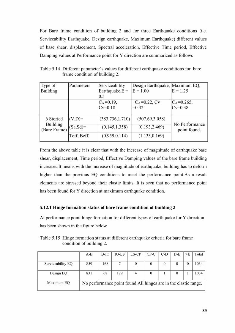
89

For Bare frame condition of building 2 and for three Earthquake conditions (i.e.

Serviceability Earthquake, Design earthquake, Maximum Earthquake) different values

of base shear, displacement, Spectral acceleration, Effective Time period, Effective

Damping values at Performance point for Y direction are summarized as follows

Table 5.14 Different parameter’s values for different earthquake conditions for bare frame condition of building 2. Type of Building




CA =0.19, Cv=0.18

CA =0.22, Cv =0.32

CA =0.265, Cv=0.38

6 Storied Building

(Bare Frame)

(V,D)= (383.736,1.710) (507.69,3.058) No Performance

point found. (Sa,Sd)= (0.145,1.358) (0.193,2.469)

Teff, Beff, (0.959,0.114) (1.133,0.169)



increases.It means with the increase of magnitude of earthquake, building has to deform

higher than the previous EQ conditions to meet the performance point.As a result

elements are stressed beyond their elastic limits. It is seen that no performance point

has been found for Y direction at maximum earthquake condition.

5.12.1 Hinge formation status of bare frame condition of building 2

At performance point hinge formation for different types of earthquake for Y direction


Table 5.15 Hinge formation status at different earthquake criteria for bare frame condition of building 2.



Design EQ 831 68 129 4 0 1 0 1 1034


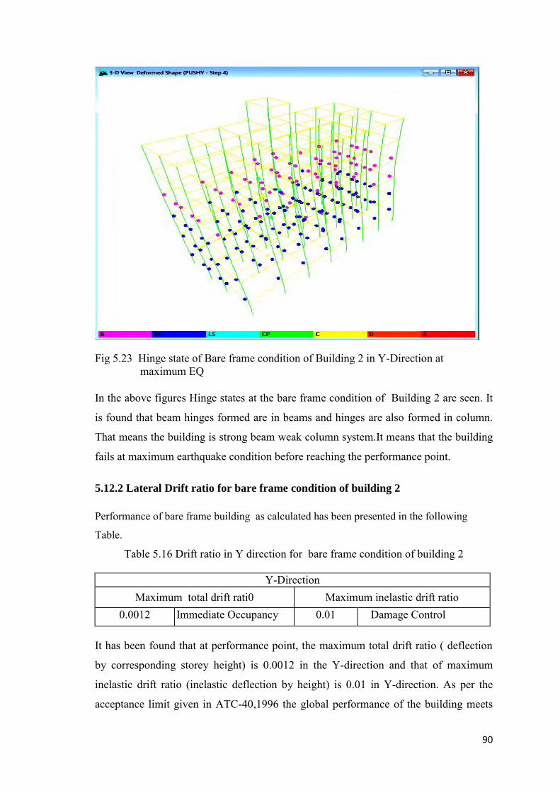
90

Fig 5.23 Hinge state of Bare frame condition of Building 2 in Y-Direction at maximum EQ In the above figures Hinge states at the bare frame condition of Building 2 are seen. It

is found that beam hinges formed are in beams and hinges are also formed in column.

That means the building is strong beam weak column system.It means that the building

fails at maximum earthquake condition before reaching the performance point. 5.12.2 Lateral Drift ratio for bare frame condition of building 2

Performance of bare frame building as calculated has been presented in the following

Table.

Table 5.16 Drift ratio in Y direction for bare frame condition of building 2

Y-Direction Maximum total drift rati0 Maximum inelastic drift ratio

0.0012 Immediate Occupancy 0.01 Damage Control It has been found that at performance point, the maximum total drift ratio ( deflection

by corresponding storey height) is 0.0012 in the Y-direction and that of maximum

inelastic drift ratio (inelastic deflection by height) is 0.01 in Y-direction. As per the


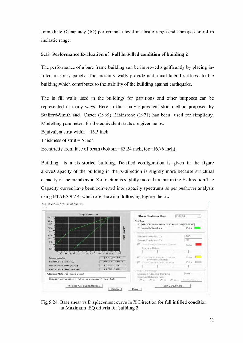
91

Immediate Occupancy (IO) performance level in elastic range and damage control in

inelastic range.

5.13 Performance Evaluation of Full In-Filled condition of building 2

The performance of a bare frame building can be improved significantly by placing in-

filled masonry panels. The masonry walls provide additional lateral stiffness to the

building,which contributes to the stability of the building against earthquake.

The in fill walls used in the buildings for partitions and other purposes can be

represented in many ways. Here in this study equivalent strut method proposed by

Stafford-Smith and Carter (1969), Mainstone (1971) has been used for simplicity.

Modelling parameters for the equivalent struts are given below

Equivalent strut width = 13.5 inch

Thickness of strut = 5 inch

Ecentricity from face of beam (bottom =83.24 inch, top=16.76 inch)

Building is a six-storied building. Detailed configuration is given in the figure

above.Capacity of the building in the X-direction is slightly more because structural

capacity of the members in X-direction is slightly more than that in the Y-direction.The

Capacity curves have been converted into capacity spectrums as per pushover analysis

using ETABS 9.7.4, which are shown in following Figures below.

Fig 5.24 Base shear vs Displacement curve in X Direction for full infilled condition at Maximum EQ criteria for building 2.

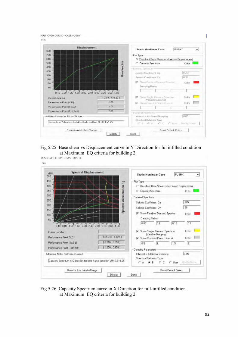
92

Fig 5.25 Base shear vs Displacement curve in Y Direction for ful infilled condition at Maximum EQ criteria for building 2.

Fig 5.26 Capacity Spectrum curve in X Direction for full-infilled condition at Maximum EQ criteria for building 2.

93

Fig 5.27 Capacity Spectrum curve in Y Direction for full infilled condition at Maximum EQ criteria for building 2. For full infilled condition of building 2 and at three Earthquake conditions (i.e.



Damping values at Performance point for Y direction are summarized as follows.

Table 5.17 Different parameter’s values at different earthquake criteria for full in-filled condition of building 2. Type of Building




CA =0.19, Cv =0.18

CA =0.22, Cv =0.32

No Performance point found. 6 Storied

Building (Full In filled

condition)

(V,D)= (432.33,1.776) (588.357,3.203)

(Sa,Sd)= (0.152,1.408) (0.208,2.574)

Teff, Beff, (0.948,0.095) (1.101,0.139) From the above table it is clear that with the increase of magnitude of earthquake base



deform higher than the previous EQ conditions to meet the performance point.As a

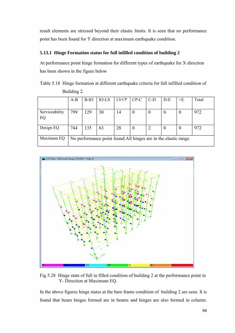
94

result elements are stressed beyond their elastic limits. It is seen that no performance

point has been found for Y direction at maximum earthquake condition.

5.13.1 Hinge Formation status for full infilled condition of building 2



Table 5.18 Hinge formation at different earthquake criteria for full infilled condition of

Building 2.


Serviceability EQ

799 129 30 14 0 0 0 0 972

Design EQ 744 135 63 28 0 2 0 0 972


Fig 5.28 Hinge state of full in filled condition of building 2 at the performance point in Y- Direction at Maximum EQ. In the above figures hinge states at the bare frame condition of building 2 are seen. It is

found that beam hinges formed are in beams and hinges are also formed in column.

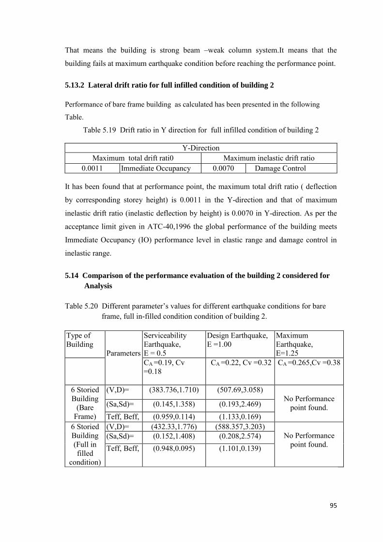
95

That means the building is strong beam –weak column system.It means that the

building fails at maximum earthquake condition before reaching the performance point. 5.13.2 Lateral drift ratio for full infilled condition of building 2

Performance of bare frame building as calculated has been presented in the following

Table.

Table 5.19 Drift ratio in Y direction for full infilled condition of building 2

Y-Direction Maximum total drift rati0 Maximum inelastic drift ratio

0.0011 Immediate Occupancy 0.0070 Damage Control It has been found that at performance point, the maximum total drift ratio ( deflection

by corresponding storey height) is 0.0011 in the Y-direction and that of maximum

inelastic drift ratio (inelastic deflection by height) is 0.0070 in Y-direction. As per the


Immediate Occupancy (IO) performance level in elastic range and damage control in

inelastic range.

5.14 Comparison of the performance evaluation of the building 2 considered for

Analysis

Table 5.20 Different parameter’s values for different earthquake conditions for bare frame, full in-filled condition condition of building 2.

Type of Building

Parameters

Serviceability Earthquake, E = 0.5


Maximum Earthquake, E=1.25

CA =0.19, Cv =0.18

CA =0.22, Cv =0.32

CA =0.265,Cv =0.38

6 Storied Building

(Bare Frame)


point found. (Sa,Sd)= (0.145,1.358) (0.193,2.469) Teff, Beff, (0.959,0.114) (1.133,0.169)

6 Storied Building (Full in filled

condition)


point found. (Sa,Sd)= (0.152,1.408) (0.208,2.574) Teff, Beff, (0.948,0.095) (1.101,0.139)

96

5.14.1 Comparison of hinge formation and base shear of building 2

Base shear at performance point and number of hinges developed up to Performance Point for Y direction at Serviceability EQ

Table 5.21 Comparison of Hinge formation and base shear for serviceability earthquake condition for a bare frame,full in-filled condition of building 2


Base Shear inKN



Bare Frame 384 859 168 7 0 0 0 0 0 1034


508 831 68 129 4 0 1 0 1 1034

Base shear at performance point and number of hinges developed up to Performance Point for Y direction at Design EQ

Table 5.22 Comparison of Hinge formation and base shear for design earthquake condition for a bare frame,full in-filled condition of building 2


Base Shear inKN


A-B B-IO I0-LS LS-CP CP-C C-D D-E >E Total

Bare Frame 433 830 65 133 5 0 1 0 0 1034

Full In-filled 588 830 65 133 4 0 1 0 1 1034

5.15 Summary

Two types of building has been analyzed in this chapter. Building 1 is an irregular building and building 2 is a regular building.

From the above tables it is clear that for building 1 the base shear developed at

performance point is lower for bare frame building than that of full in-filled frame and

soft storey frame because of less mass in stories due to absence of infill.For building 2

the findings are same, except the fact that no soft story condition has been analyzed.

Building’s natural period(T) is less than that of bare frame which means masonry infill

contributes for stiffness of the building.

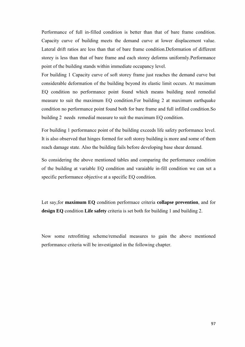
97

Performance of full in-filled condition is better than that of bare frame condition.

Capacity curve of building meets the demand curve at lower displacement value.

Lateral drift ratios are less than that of bare frame condition.Deformation of different

storey is less than that of bare frame and each storey deforms uniformly.Performance

point of the building stands within immediate occupancy level.

For building 1 Capacity curve of soft storey frame just reaches the demand curve but

considerable deformation of the building beyond its elastic limit occurs. At maximum

EQ condition no performance point found which means building need remedial

measure to suit the maximum EQ condition.For building 2 at maximum earthquake

condition no performance point found both for bare frame and full infilled condition.So

building 2 needs remedial measure to suit the maximum EQ condition.

For building 1 performance point of the building exceeds life safety performance level.

It is also observed that hinges formed for soft storey building is more and some of them

reach damage state. Also the building fails before developing base shear demand.

So considering the above mentioned tables and comparing the performance condition

of the building at variable EQ condition and varaiable in-fill condition we can set a

specific performance objective at a specific EQ condition.

Let say,for maximum EQ condition performace criteria collapse prevention, and for

design EQ condition Life safety criteria is set both for building 1 and building 2.

Now some retrofitting scheme/remedial measures to gain the above mentioned

performance criteria will be investigated in the following chapter.

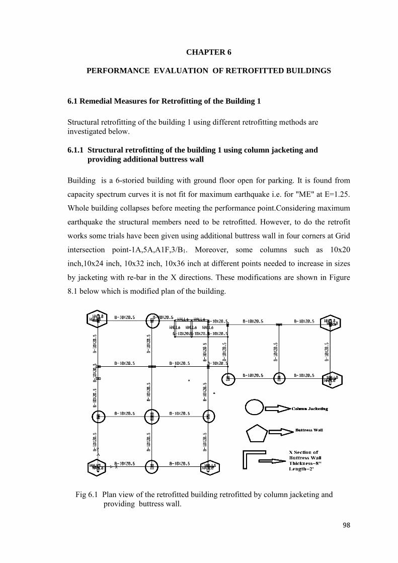
98

CHAPTER 6

PERFORMANCE EVALUATION OF RETROFITTED BUILDINGS

6.1 Remedial Measures for Retrofitting of the Building 1

Structural retrofitting of the building 1 using different retrofitting methods are investigated below. 6.1.1 Structural retrofitting of the building 1 using column jacketing and

providing additional buttress wall

Building is a 6-storied building with ground floor open for parking. It is found from

capacity spectrum curves it is not fit for maximum earthquake i.e. for "ME" at E=1.25.

Whole building collapses before meeting the performance point.Considering maximum

earthquake the structural members need to be retrofitted. However, to do the retrofit

works some trials have been given using additional buttress wall in four corners at Grid

intersection point-1A,5A,A1F,3/B1. Moreover, some columns such as 10x20

inch,10x24 inch, 10x32 inch, 10x36 inch at different points needed to increase in sizes

by jacketing with re-bar in the X directions. These modifications are shown in Figure

8.1 below which is modified plan of the building.

Fig 6.1 Plan view of the retrofitted building retrofitted by column jacketing and providing buttress wall.

99

6.1.1.1 Performance evaluation of retrofitted building 1 retrofitted with column

jacketing and buttress wall.

The revised well defined capacity curves have been found based on the retrofit building

in two orthogonal directions, which are shown in the following Figures 8.2 and 8.3.

Capacity of the building in the X-direction is slightly more because structural capacity

of the members in X-direction is slightly more than that in the Y-direction.

Fig 6.2 Base shear vs Displacement curve in X Direction for retrofitted Building 1(with buttress wall and column jacketing at Maximum EQ Condition.

Fig 6.3 Base shear vs Displacement curve in Y Direction for retrofitted building 1 (with buttress wall and column jacketing at Maximum EQ Condition.

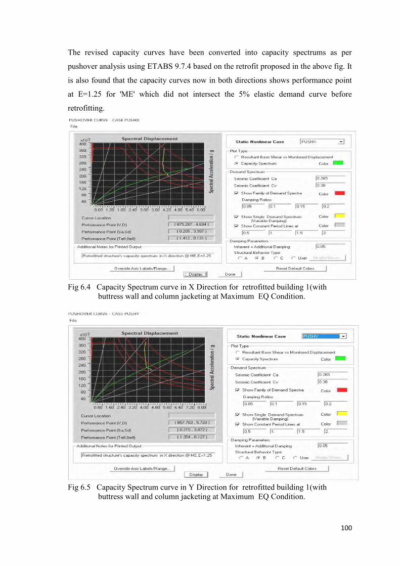
100

The revised capacity curves have been converted into capacity spectrums as per

pushover analysis using ETABS 9.7.4 based on the retrofit proposed in the above fig. It

is also found that the capacity curves now in both directions shows performance point

at E=1.25 for 'ME' which did not intersect the 5% elastic demand curve before

retrofitting.

Fig 6.4 Capacity Spectrum curve in X Direction for retrofitted building 1(with buttress wall and column jacketing at Maximum EQ Condition.

Fig 6.5 Capacity Spectrum curve in Y Direction for retrofitted building 1(with buttress wall and column jacketing at Maximum EQ Condition.

101

For the retrofitted building 1(with buttress wall and column jacketing) and for three

Earthquake conditions (i.e. Serviceability Earthquake,Designearthquake,Maximum

Earthquake) different values of base shear,displacement,Spectralacceleration,Effective

Time period, Effective Damping values at Performance point for X direction are

summarised as follows

Table 6.1 Different parameter’s values for different earthquake conditions for the retrofitted building 1 retrofitted with buttress wall and column jacketing. Type of Building




CA =0.19, Cv =0.18

CA =0.22, Cv =0.32

CA =0.265, Cv =0.38

6 Storied Building

(Retrofitted with buttress wall and

column jacketing)

(V,D)= (554.473,2.144) (781.294,3.868) (875.287,4.694)

(Sa,Sd)= (0.123,1.793) (0.179,3.275) (0.205,3.997)

Teff, Beff, (1.216,0.096) (1.362,0.127) (1.412,0.131)

6.1.1.2 Hinge formation status of the retrofitted building 1 retrofitted with

buttress wall and column jacketing


Table 6.2 Hinge formation for different earthquake conditions for the retrofitted building 1 retrofitted with buttress wall and column jacketing. A-B B-IO IO-

LS LS-CP

CP-C C-D D-E >E Total

Serviceability

EQ

773 143 30 8 0 0 0 0 954

Design EQ 704 157 63 30 0 0 0 0 954

Maximum EQ 699 155 64 35 1 0 0 0 954

102

Fig 6.6 Hinge state of retrofitted building 1 with buttress wall and column jacketing at the performance point in X-Direction at Maximum EQ.

6.1.1.3 Lateral drift ratio of the retrofitted building 1 retrofitted with

buttress wall and column jacketing

Lateral drift ratio of the retrofitted building 1 retrofitted with buttress wall and column jacketing is shown in the table below

Table 6.3 Drift ratio in X direction for retrofitted building 1retrofitted with buttress wall and column jacketing

At Performance Point X-Direction (Retrofitted building with buttress wall and column jacketing) Maximum total drift rati0 Maximum inelastic drift ratio

0.0027 Immediate Occupancy 0.019 Life Safety

6.1.2 Structural retrofitting of the building 1 using insertion of additional shear

wall

Building is a 6-storied building with ground floor open for parking. It is found from

capacity spectrum curves it is not fit for maximum earthquake i.e. for "ME" at E=1.25.

Whole building collapses before meeting the performance point.Considering maximum

earthquake the structural members need to be retrofitted. However, to do the retrofit

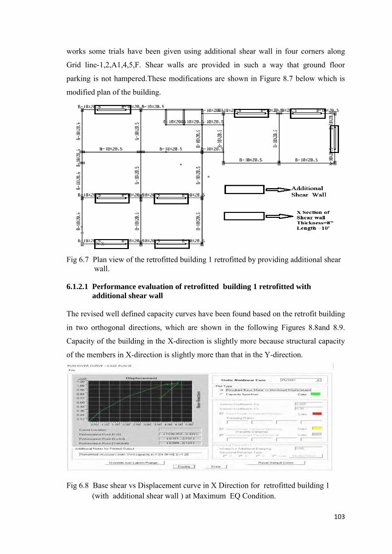
103

works some trials have been given using additional shear wall in four corners along

Grid line-1,2,A1,4,5,F. Shear walls are provided in such a way that ground floor

parking is not hampered.These modifications are shown in Figure 8.7 below which is

modified plan of the building.

Fig 6.7 Plan view of the retrofitted building 1 retrofitted by providing additional shear wall.

6.1.2.1 Performance evaluation of retrofitted building 1 retrofitted with

additional shear wall


in two orthogonal directions, which are shown in the following Figures 8.8and 8.9.



Fig 6.8 Base shear vs Displacement curve in X Direction for retrofitted building 1 (with additional shear wall ) at Maximum EQ Condition.

104

Fig 6.9 Base shear vs Displacement curve in Y Direction for retrofitted building 1(with additional shear wall ) at Maximum EQ Condition. The revised capacity curves have been converted into capacity spectrums as per




retrofitting.

Fig 6.10 Capacity Spectrum curve in X Direction for retrofitted building 1 (with additional shear wall ) at Maximum EQ Condition.

105

Fig 6.11 Capacity Spectrum curve in Y Direction for retrofitted building 1(with additional shear wall ) at Maximum EQ Condition. For the retrofitted building 1(with additional shear wall) and for three Earthquake

conditions (i.e. Serviceability Earthquake,Designearthquake,Maximum Earthquake)

different values of base shear,displacement,spectralacceleration, effective time period,

effective Damping values at Performance point for X direction are summarised as

follows

Table 6.4 Different parameter’s values for different earthquake conditions for retrofitted building 1 retrofitted with additional shear wall. Type of Building




CA =0.19,Cv =0.18

CA =0.22, Cv =0.32

CA =0.265,Cv =0.38

6 Storied Building

(Retrofitted with

additional shear wall)

(V,D)= (637.882,1.568) (928.715,2.787) (1036.919,3.33)

(Sa,Sd)= (0.181,1.257) (0.274,2.275) (0.311,2.737)

Teff, Beff (0.823,0.087) (0.914,0.114) (0.949,0.123)

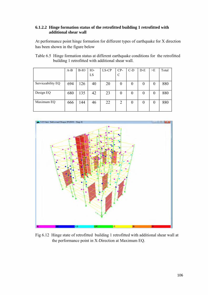
106

6.1.2.2 Hinge formation status of the retrofitted building 1 retrofitted with

additional shear wall


Table 6.5 Hinge formation status at different earthquake conditions for the retrofitted building 1 retrofitted with additional shear wall. A-B B-IO IO-

LS LS-CP CP-

C C-D D-E >E Total


Design EQ 680 135 42 23 0 0 0 0 880

Maximum EQ 666 144 46 22 2 0 0 0 880

Fig 6.12 Hinge state of retrofitted building 1 retrofitted with additional shear wall at the performance point in X-Direction at Maximum EQ.

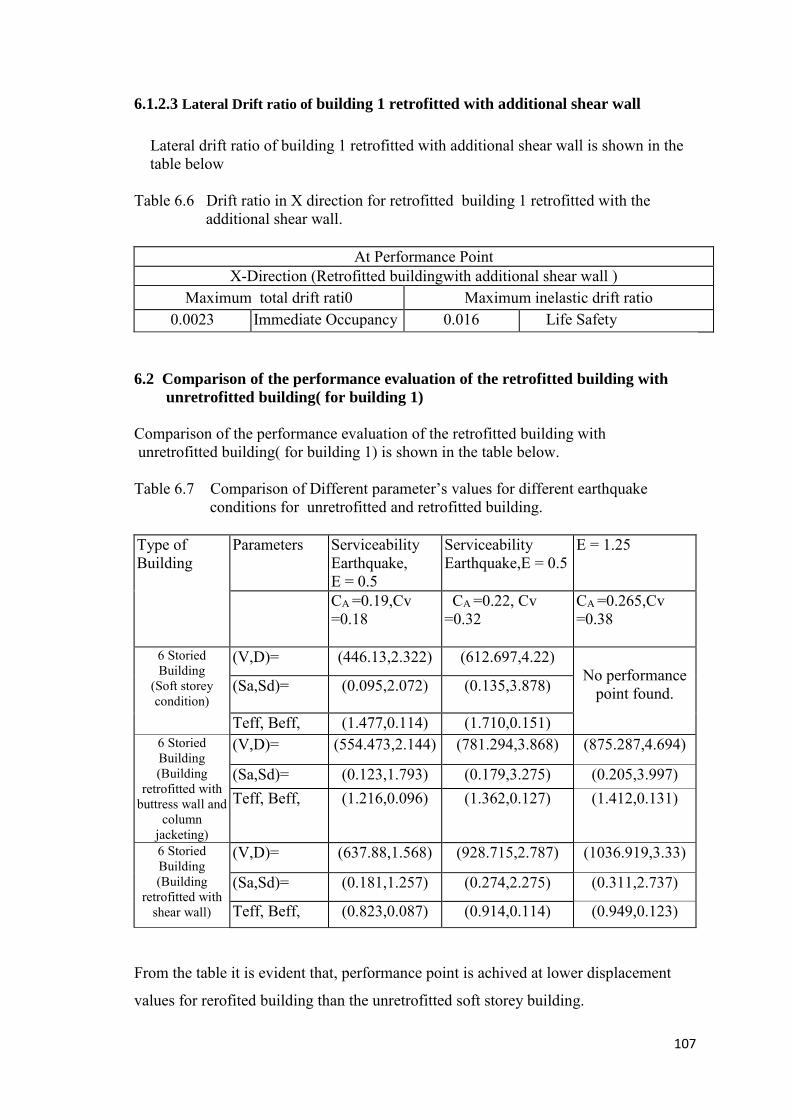
107

6.1.2.3 Lateral Drift ratio of building 1 retrofitted with additional shear wall

Lateral drift ratio of building 1 retrofitted with additional shear wall is shown in the table below Table 6.6 Drift ratio in X direction for retrofitted building 1 retrofitted with the additional shear wall.

At Performance Point X-Direction (Retrofitted buildingwith additional shear wall )

Maximum total drift rati0 Maximum inelastic drift ratio 0.0023 Immediate Occupancy 0.016 Life Safety

6.2 Comparison of the performance evaluation of the retrofitted building with

unretrofitted building( for building 1)

Comparison of the performance evaluation of the retrofitted building with unretrofitted building( for building 1) is shown in the table below.

Table 6.7 Comparison of Different parameter’s values for different earthquake conditions for unretrofitted and retrofitted building. Type of Building


Serviceability Earthquake,E = 0.5

E = 1.25

CA =0.19,Cv =0.18

CA =0.22, Cv =0.32

CA =0.265,Cv =0.38

6 Storied Building

(Soft storey condition)


point found. (Sa,Sd)= (0.095,2.072) (0.135,3.878)

Teff, Beff, (1.477,0.114) (1.710,0.151) 6 Storied Building (Building

retrofitted with buttress wall and

column jacketing)

(V,D)= (554.473,2.144) (781.294,3.868) (875.287,4.694)

(Sa,Sd)= (0.123,1.793) (0.179,3.275) (0.205,3.997) Teff, Beff, (1.216,0.096) (1.362,0.127) (1.412,0.131)

6 Storied Building (Building

retrofitted with shear wall)

(V,D)= (637.88,1.568) (928.715,2.787) (1036.919,3.33)

(Sa,Sd)= (0.181,1.257) (0.274,2.275) (0.311,2.737)

Teff, Beff, (0.823,0.087) (0.914,0.114) (0.949,0.123)

From the table it is evident that, performance point is achived at lower displacement

values for rerofited building than the unretrofitted soft storey building.

108

6.2.1 Comparison of hinge formation status of the retrofitted building with

unretrofitted building( for building 1)

At performance point hinge formation for different types of earthquake for X direction has been shown in the table below.

Table 6.8 Comparison of Base shear and Hinge formation at performance point and number of hinges developed up to performance point for X direction for Design EQ.


Base Shear inKN



Soft Storey Frame 613 683 144 64 30 0 1 0 0 922

Retrofitted Building (with buttress wall

and column jacketing)

781 704 157 63 30 0 0 0 0 954

Retrofitted Building (with shear wall)

929 680 135 42 23 0 0 0 0 880

Table 6.9 Comparison of Base shear and Hinge formation at performance point and number of hinges developed up to performance point for X direction for Maximum EQ.


Base Shear inKN



Soft Storey Frame No performance point found.Building totally collapses before reaching the performance point.



875 699 155 64 35 1 0 0 0 954

Retrofitted Building (with shear wall)

1037 666 144 46 22 2 0 0 0 880

From the above table it is evident that hinges formed in the retrofitted building for

design EQ condition do not cross the life safety range,and for maximum EQ it does not

cross the collapse prevention range.

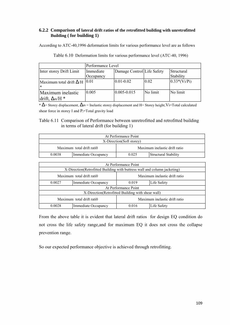
109

6.2.2 Comparison of lateral drift ratios of the retrofitted building with unretrofitted

Building ( for building 1)

According to ATC-40,1996 deformation limits for various performance level are as follows

Table 6.10 Deformation limits for various performance level (ATC-40, 1996) Performance Level Inter storey Drift Limit Immediate

Occupancy Damage Control Life Safety Structural

Stability Maximum total drift Δ/H *

0.01 0.01-0.02 0.02 0.33*(Vi/Pi)



* Δ= Storey displacement, Δin = Inelastic storey displacement and H= Storey height,Vi=Total calculated shear force in storey I and Pi=Total gravity load

Table 6.11 Comparison of Performance between unretrofitted and retrofitted building in terms of lateral drift (for building 1)

At Performance Point X-Direction(Soft storey)


0.0038 Immediate Occupancy 0.025 Structural Stability

At Performance Point X-Direction(Retrofitted Building with buttress wall and column jacketing)


0.0027 Immediate Occupancy 0.019 Life Safety At Performance Point

X-Direction(Retrofitted Building with shear wall)


0.0028 Immediate Occupancy 0.016 Life Safety From the above table it is evident that lateral drift ratios for design EQ condition do

not cross the life safety range,and for maximum EQ it does not cross the collapse

prevention range.

So our expected performance objective is achieved through retrofitting.

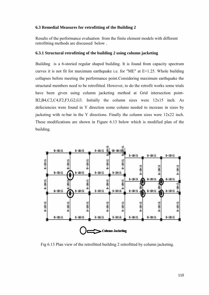
110

6.3 Remedial Measures for retrofitting of the Building 2

Results of the performance evaluation from the finite element models with different retrofitting methods are discussed below .

6.3.1 Structural retrofitting of the building 2 using column jacketing

Building is a 6-storied regular shaped building. It is found from capacity spectrum

curves it is not fit for maximum earthquake i.e. for "ME" at E=1.25. Whole building

collapses before meeting the performance point.Considering maximum earthquake the

structural members need to be retrofitted. However, to do the retrofit works some trials

have been given using column jacketing method at Grid intersection point-

B2,B4,C2,C4,F2,F3,G2,G3. Initially the column sizes were 12x15 inch. As

defeciencies were found in Y direction some colums needed to increase in sizes by

jacketing with re-bar in the Y directions. Finally the column sizes were 12x22 inch.

These modifications are shown in Figure 6.13 below which is modified plan of the

building.

Fig 6.13 Plan view of the retrofitted building 2 retrofitted by column jacketing.

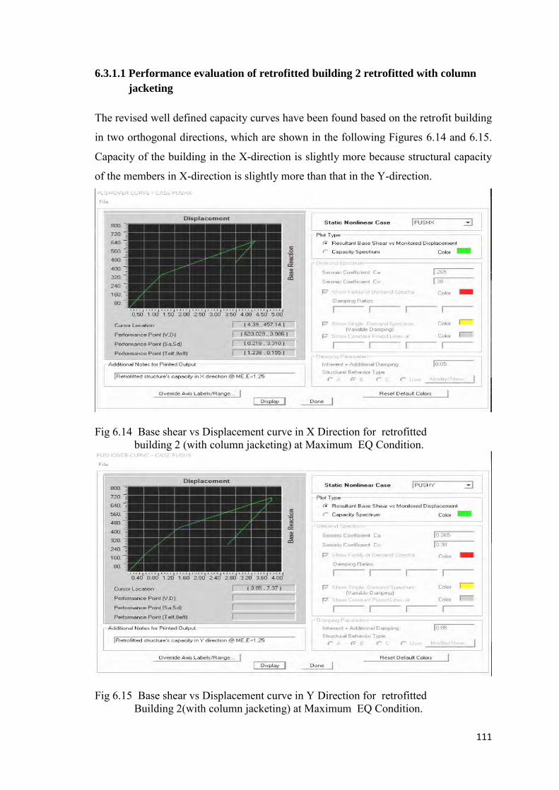
111


jacketing





Fig 6.14 Base shear vs Displacement curve in X Direction for retrofitted building 2 (with column jacketing) at Maximum EQ Condition.

Fig 6.15 Base shear vs Displacement curve in Y Direction for retrofitted Building 2(with column jacketing) at Maximum EQ Condition.

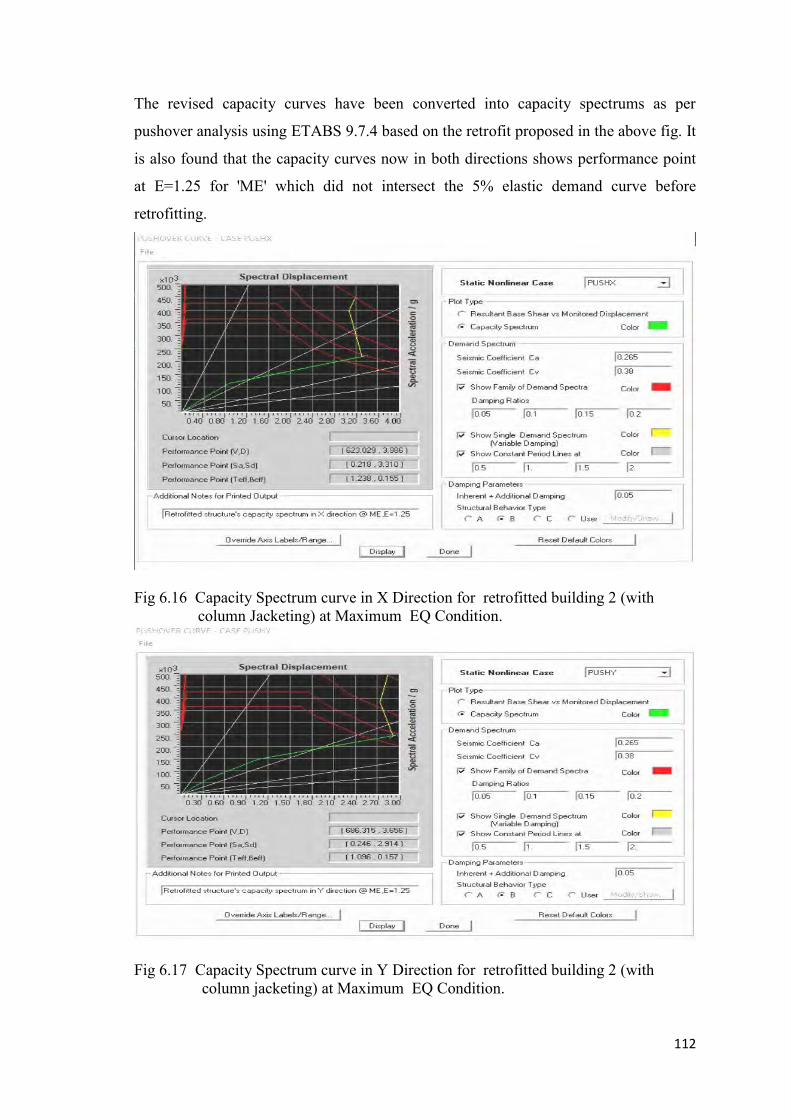
112





retrofitting.

Fig 6.16 Capacity Spectrum curve in X Direction for retrofitted building 2 (with column Jacketing) at Maximum EQ Condition.

Fig 6.17 Capacity Spectrum curve in Y Direction for retrofitted building 2 (with column jacketing) at Maximum EQ Condition.

113

For the retrofitted building 2(with column jacketing) and for three Earthquake

conditions (i.e. Serviceability Earthquake, Design earthquake, Maximum Earthquake)

different values of base shear, displacement, Spectral acceleration, Effective Time

period, Effective Damping values at Performance point for Y direction are summarized

as follows

Table 6.12 Different parameter’s values for different earthquake conditions for the retrofitted building 2 retrofitted with column jacketing. Type of Building




CA =0.19, Cv =0.18

CA =0.22, Cv =0.32

CA =0.265, Cv =0.38

6 Storied Building

(Retrofitted with column

jacketing)

(V,D)= (451.721,1.660) (613.284,3.035) (686.315,3.656)

(Sa,Sd)= (0.162,1.309) (0.220,2.414) (0.246,2.914)

Teff, Beff, (0.887,0.096) (1.031,0.138) (1.096,0.157)

6.3.1.2 Hinge formation status of the retrofitted structure 2 retrofitted with

column jacketing

At performance point hinge formation for different types of earthquake for Y direction has been shown in the figure below

Table 6.13 Hinge formation for different earthquake conditions for the retrofitted building 2 retrofitted with column jacketing. A-B B-IO IO-LS LS-CP CP-C C-D D-E >E Total


Design EQ 1262 86 138 6 2 0 0 0 1492

Maximum EQ 1262 86 136 6 1 1 0 0 1492

114

Fig 6.18 Hinge state of retrofitted building 2 retrofitted with column jacketing at the performance point in Y-Direction at Maximum EQ. 6.3.1.3 Lateral drift ratio of the retrofitted building 2 retrofitted with column

Jacketing

Lateral drift ratio of the retrofitted building 2 retrofitted with column jacketing is shown in the table below. Table 6.14 Drift ratio in Y direction for retrofitted building with column jacketing

At Performance Point Y-Direction (Building retrofitted with column jacketing)

Maximum total drift rati0 Maximum inelastic drift ratio 0.0010 Immediate Occupancy 0.0068 Damage Control

6.3.2 Structural retrofitting of the building 2 using column jacketing and buttress

wall




structural members need to be retrofitted. However, to do the retrofit works another

option such as column jacketing with buttress wall will be trialed this time as only

column jacketing method did not give satisfactory performance result.Additional

buttress wall in four corners at grid intersections point-A6,A1,H1,H5 along with

retrofitted columns at grid intersection point-B2,B4,C2,C4,F2,F3,G2,G3 are placed.

115

Initially the column sizes were 12x15 inch. As defeciencies were found in Y direction

some colums needed to increase in sizes by jacketing with re-bar in the Y directions.

Finally the column sizes were 12x20 inch. The thickness of the buttress wall is 8 inch

and it is placed upto 2nd floor.These modifications are shown in Figure 6.19 below.

Fig 6.19 Plan view of the retrofitted building 2 retrofitted by column jacketing and buttress wall. 6.3.2.1 Performance evaluation of retrofitted building 2 retrofitted with column

jacketing and buttress wall





Fig 6.20 Base shear vs Displacement curve in X Direction for retrofitted Building 2 (with column jacketing and buttress wall) at Maximum EQ Condition.

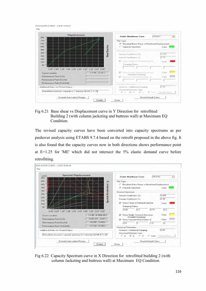
116

Fig 6.21 Base shear vs Displacement curve in Y Direction for retrofitted Building 2 (with column jacketing and buttress wall) at Maximum EQ Condition. The revised capacity curves have been converted into capacity spectrums as per




retrofitting.

Fig 6.22 Capacity Spectrum curve in X Direction for retrofitted building 2 (with column Jacketing and buttress wall) at Maximum EQ Condition.

117

Fig 6.23 Capacity Spectrum curve in Y Direction for retrofitted building 2 (with column jacketing and buttress wall) at Maximum EQ Condition. For the retrofitted building 2 (with column jacketing) and for three Earthquake

conditions (i.e. Serviceability Earthquake,Designearthquake,Maximum Earthquake)

different values of base shear,displacement,Spectralacceleration,Effective Time period,

Effective Damping values at Performance point for Y direction are summarised as

follows

Table 6.15 Different parameter’s values for different earthquake conditions for the retrofitted building 2 retrofitted with column jacketing and buttress wall. Type of Building




CA =0.19, Cv =0.18

CA =0.22, Cv =0.32

CA =0.265, Cv =0.38

6 Storied Building

(Retrofitted with column jacketing and buttress wall)

(V,D)= (480.08,1.584) (652.91,2.89) (730.497,3.477)

(Sa,Sd)= (0.176,1.239) (0.241,2.275) (0.270,2.740)

Teff, Beff, (0.827,0.092) (0.953,0.131) (1.010,0.148)

118

6.3.2.2 Hinge formation status of the retrofitted structure 2 retrofitted with

Buttress wall and column jacketing

At performance point hinge formation for different types of earthquake for Y direction has been shown in the figure below

Table 6.16 Hinge formation for different earthquake conditions for the retrofitted building 2 retrofitted with column jacketing and buttress wall.



Design EQ 1250 119 120 3 0 0 0 0 1492

Maximum EQ 1250 119 119 4 1 0 0 0 1492

Fig 6.24 Hinge state of retrofitted building 2 retrofitted with column jacketing and buttress wall at the performance point in Y-Direction at Maximum EQ.

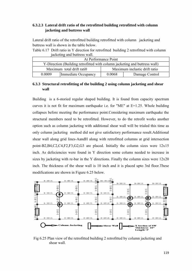
119

6.3.2.3 Lateral drift ratio of the retrofitted building retrofitted with column


Lateral drift ratio of the retrofitted building retrofitted with column jacketing and buttress wall is shown in the table below. Table 6.17 Drift ratio in Y direction for retrofitted building 2 retrofitted with column jacketing and buttress wall.

At Performance Point Y-Direction (Building retrofitted with column jacketing and buttress wall)


6.3.3 Structural retrofitting of the building 2 using column jacketing and shear

wall




structural members need to be retrofitted. However, to do the retrofit works another

option such as column jacketing with additional shear wall will be trialed this time as

only column jacketing method did not give satisfactory performance result.Additional

shear wall along grid lines-AandH along with retrofitted columns at grid intersection

point-B2,B4,C2,C4,F2,F3,G2,G3 are placed. Initially the column sizes were 12x15

inch. As defeciencies were found in Y direction some colums needed to increase in

sizes by jacketing with re-bar in the Y directions. Finally the column sizes were 12x20

inch. The thickness of the shear wall is 10 inch and it is placed upto 3rd floor.These

modifications are shown in Figure 6.25 below.

Fig 6.25 Plan view of the retrofitted building 2 retrofitted by column jacketing and shear wall.

120







Fig 6.26 Base shear vs Displacement curve in X Direction for retrofitted Building 2(with column jacketing and shear wall) at Maximum EQ Condition.

Fig 6.27 Base shear vs Displacement curve in Y Direction for retrofitted Building 2 (with column jacketing and shear wall) at Maximum EQ Condition.

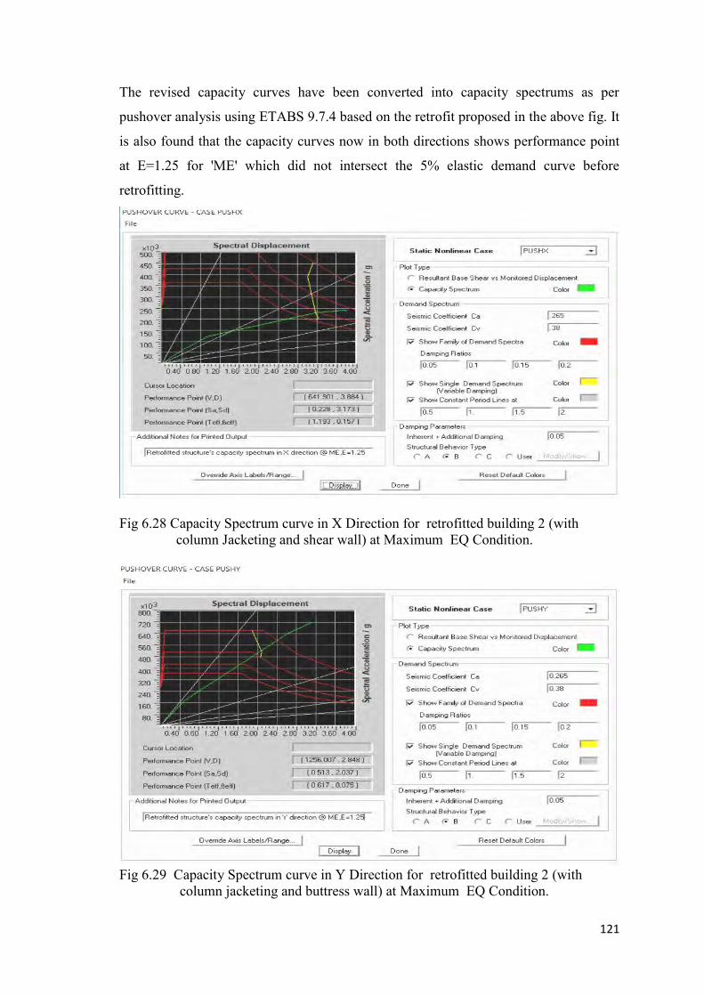
121





retrofitting.

Fig 6.28 Capacity Spectrum curve in X Direction for retrofitted building 2 (with column Jacketing and shear wall) at Maximum EQ Condition.

Fig 6.29 Capacity Spectrum curve in Y Direction for retrofitted building 2 (with column jacketing and buttress wall) at Maximum EQ Condition.

122

For the retrofitted building 2 (with column jacketing and shear wall) and for three

Earthquake conditions (i.e. Serviceability Earthquake,Designearthquake,Maximum

Earthquake) different values of base shear,displacement,Spectralacceleration,Effective

Time period, Effective Damping values at Performance point for Y direction are

summarised as follows

Table 6.18 Different parameter’s values for different earthquake conditions for the retrofitted building 2 retrofitted with column jacketing and shear wall . Type of Building




CA =0.19, Cv =0.18

CA =0.22, Cv =0.32

CA =0.265, Cv =0.38

6 Storied Building

(Retrofitted with column jacketing and buttress wall)

(V,D)= (677.234,1.322) (1062.763,2.339) (1256.007,2.848)

(Sa,Sd)= (0.275,0.960) (0.434,1.678) (0.513,2.037)

Teff, Beff, (0.564,0.057) (0.599,0.069) (0.617,0.075)

6.3.3.2 Hinge formation status of the retrofitted building 2 retrofitted with shear

wall and column jacketing

At performance point hinge formation for different types of earthquake for Y direction has been shown in the figure below.

Table 6.19 Hinge formation status of the retrofitted building 2 retrofitted with shear wall and column jacketing


Serviceability

EQ

1150 177 83 10 0 0 0 0 1420

Design EQ 1116 125 157 22 0 0 0 0 1420

Maximum EQ 1116 125 157 21 1 0 0 0 1420

123

Fig 6.30 Hinge state of retrofitted building 2 retrofitted with column jacketing and shear wall at the performance point in Y-Direction at Maximum EQ. 6.3.3.3 Lateral drift ratio of the retrofitted building 2 retrofitted with column

jacketing and shear wall

Lateral drift ratio of the retrofitted building 2 retrofitted with column jacketing and shear wall is shown in the following table Table 6.20 Drift ratio in Y direction for retrofitted building 2 with column jacketing and shear wall

At Performance Point Y-Direction (Building retrofitted with column jacketing and buttress wall) Maximum total drift rati0 Maximum inelastic drift ratio

0.0005 Immediate Occupancy

0.0060 Damage Control

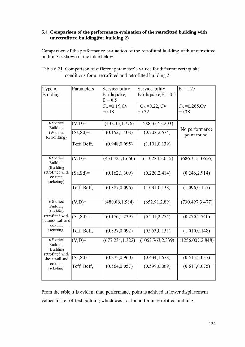
124

6.4 Comparison of the performance evaluation of the retrofitted building with

unretrofitted building(for building 2)

Comparison of the performance evaluation of the retrofitted building with unretrofitted building is shown in the table below. Table 6.21 Comparison of different parameter’s values for different earthquake conditions for unretrofitted and retrofitted building 2.

Type of Building


Serviceability Earthquake,E = 0.5

E = 1.25

CA =0.19,Cv =0.18

CA =0.22, Cv =0.32

CA =0.265,Cv =0.38

6 Storied Building (Without

Retrofitting)


point found. (Sa,Sd)= (0.152,1.408) (0.208,2.574)

Teff, Beff, (0.948,0.095) (1.101,0.139)


retrofitted with column

jacketing)

(V,D)= (451.721,1.660) (613.284,3.035) (686.315,3.656)

(Sa,Sd)= (0.162,1.309) (0.220,2.414) (0.246,2.914)

Teff, Beff, (0.887,0.096) (1.031,0.138) (1.096,0.157)


retrofitted with buttress wall and

column jacketing)

(V,D)= (480.08,1.584) (652.91,2.89) (730.497,3.477)

(Sa,Sd)= (0.176,1.239) (0.241,2.275) (0.270,2.740)

Teff, Beff, (0.827,0.092) (0.953,0.131) (1.010,0.148)


retrofitted with shear wall and

column jacketing)

(V,D)= (677.234,1.322) (1062.763,2.339) (1256.007,2.848)

(Sa,Sd)= (0.275,0.960) (0.434,1.678) (0.513,2.037)

Teff, Beff, (0.564,0.057) (0.599,0.069) (0.617,0.075)

From the table it is evident that, performance point is achived at lower displacement

values for retrofitted building which was not found for unretrofitted building.

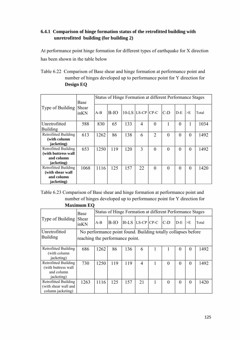
125

6.4.1 Comparison of hinge formation status of the retrofitted building with

unretrofitted building (for building 2)


has been shown in the table below

Table 6.22 Comparison of Base shear and hinge formation at performance point and number of hinges developed up to performance point for Y direction for Design EQ

Type of Building Base Shear inKN



Unretrofitted Building

588 830 65 133 4 0 1 0 1 1034

Retrofitted Building

(with column

jacketing)

613 1262 86 138 6 2 0 0 0 1492


(with buttress wall

and column

jacketing)

653 1250 119 120 3 0 0 0 0 1492


(with shear wall

and column

jacketing)

1068 1116 125 157 22 0 0 0 0 1420

Table 6.23 Comparison of Base shear and hinge formation at performance point and number of hinges developed up to performance point for Y direction for Maximum EQ

Type of Building Base Shear inKN


A-B B-IO I0-LS LS-CP CP-C C-D D-E >E Total

Unretrofitted Building

No performance point found. Building totally collapses before reaching the performance point.

Retrofitted Building (with column

jacketing)

686 1262 86 136 6 1 1 0 0 1492



730 1250 119 119 4 1 0 0 0 1492

Retrofitted Building (with shear wall and column jacketing)

1263 1116 125 157 21 1 0 0 0 1420

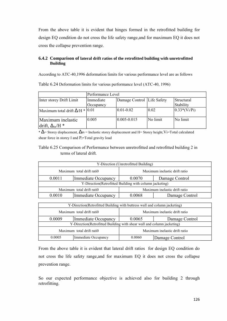
126

From the above table it is evident that hinges formed in the retrofitted building for

design EQ condition do not cross the life safety range,and for maximum EQ it does not

cross the collapse prevention range.

6.4.2 Comparison of lateral drift ratios of the retrofitted building with unretrofitted

Building

According to ATC-40,1996 deformation limits for various performance level are as follows Table 6.24 Deformation limits for various performance level (ATC-40, 1996) Performance Level Inter storey Drift Limit Immediate

Occupancy Damage Control Life Safety Structural

Stability Maximum total drift Δ/H * 0.01 0.01-0.02 0.02 0.33*(Vi/Pi)



* Δ= Storey displacement, Δin = Inelastic storey displacement and H= Storey height,Vi=Total calculated shear force in storey I and Pi=Total gravity load

Table 6.25 Comparison of Performance between unretrofitted and retrofitted building 2 in terms of lateral drift.

Y-Direction (Unretrofitted Building)


0.0011 Immediate Occupancy 0.0070 Damage Control Y-Direction(Retrofitted Building with column jacketing)


Y-Direction(Retrofitted Building with buttress wall and column jacketing)


0.0009 Immediate Occupancy 0.0065 Damage Control Y-Direction(Retrofitted Building with shear wall and column jacketing)


0.0005 Immediate Occupancy 0.0060 Damage Control From the above table it is evident that lateral drift ratios for design EQ condition do

not cross the life safety range,and for maximum EQ it does not cross the collapse

prevention range.

So our expected performance objective is achieved also for building 2 through retrofitting.

127

CHAPTER 7

CONCLUSIONS AND RECOMMENDATIONS

7.1 General

For understanding the performance of building under different seismic conditions

pushover analysis has now been considered as an effective tool which is a vast

nonlinear analysis method. There are some desired levels of seismic performance when

the building is subjected to specific levels of seismic ground motion. Acceptable

performance is measured by the level of structural and/or nonstructural damage

expected from the earthquake excitation.

The main goal of the study was to evaluate the adequacy and seismic performance of

conventionally designed typical bare frame, fully in-filled, soft ground storey condition

of buildings with the help of pushover curve (capacity curve) under earthquake

loading. Another goal of the study was to identify the deficiencies in the seismic

performance of the building and to see whether any performance improvement is

required or not after the pushover analysis, by using a finite element software. Two

types of building were analyzed in this thesis. Building 1 is an irregular shaped office

building and building 2 is a regular shaped residential building.Bare,in-filled frame and

soft storey condition of the buildings were considered and their seismic performance

was evaluated in a detailed way. Two specific performance criteria were selected (i.e.

Life safety, collapse prevention) for two specific earthquake condition(i.e. Design

Earthquake, Maximum earthquake).In order to gain those performance objectives some

retrofitting measures were applied and the performance of the particular building was

evaluated and was found satisfactory.

7.2 Findings of The Study

Within the scope of this study the main conclusions can be summarized as follows

(i) For building 1 Base shear developed at performance point is 20% lower for

bare frame condition than that of full in-filled frame condition and 12.1% lower

than soft storey frame condition because of less mass in stories due to absence

of infill. For building 2 base shear developed at performance point is 12.7%

lower for bare frame condition than that of full in-filled frame condition.

128

(ii) For both the buildings (1 and 2) natural period (T) is less than that of bare frame

which means masonry infill contributes for stiffness of the building.

(iii) Seismic performance of full in-filled frame condition is better than that of bare

frame condition. Capacity curve of both the buildings meets the demand curve at

lower displacement value. Lateral drift ratios are 4 % less than that of bare frame

condition of building 1.Performance point of the building stands within immediate

occupancy level.For realistic modelling, infill has been considered and better

performance is found than bare frame.

(iv) The addition to infill in the upper stories leaving the ground floor open makes soft

storey case which can be fatal for earthquake. The seismic performance of

buildings having soft ground stories are very poor during earthquake shaking. In

most of the cases building collapses due to failure of ground storey columns before

reaching performance point. As open ground storey is unavoidable considering the

functional requirement, alternative measures need to be adopted for this specific

situation for reduction of vulnerability and achieve acceptable performances. The

performances can be improved through improved systems which would improve

stiffness of the ground floor and reduce the otherwise excessive ductility demand

of the soft storey.

(v) For the three types of buildings considered (bare, full in-filled, soft ground

storey),roof displacement is highest for bare frame and ground floor displacement

is highest for soft storey.

(vi) Top and bottom corners of the column are most vulnerable point since strut action

of infill imposes a concentrated load at these joints. So special detailing

considerations should be adopted.

(vii) The performance evaluation of the case study buildings (soft storey condition for

building 1 and full infilled condition for building 2) indicate that it does not show

any performance point at Maximum Earthquake (ME), that means it totally

collapses and at Design Earthquake (DE) condition, hinges formed crosses the

collapse prevention level. So, the building is retrofitted with some available

retrofitting schemes such as column jacketing with buttress wall and insertion of

shear wall.Evaluating the performance after retrofitting it is found that the

specified building satisfies the "Life safety" performance criteria for the Design

Earthquake (DE) and ''Collapse prevention (CP)" criteria for Maximum Earthquake

(ME).

129

(viii) Among the considered retrofitting measures "insertion of shear wall" shows better

performance over "column jacketing with buttress wall" in terms of lateral inelastic

drift ratio and number of hinges formed for building 1. For building 2 retrofitting

measure “shear wall with column jacketing” shows better performance over

"column jacketing with buttress wall" and "column jacketing” in terms of lateral

inelastic drift ratio and no of hinges formed. But "insertion of shear wall" creates

some problems too such as restricted parking facilities in the ground floor.

7.3 Recommendations for Future Studies

Considering the limitations, the following recommendations for further study can be

made from the present study

(i) The thesis concentrated its study mainly on a medium rise building.

Performance study on high rise buildings can be studied further.

(ii) The effect of type of foundation and soil on earthquake response of a building

can be investigated.

(iii) Verification of the proposed remedial measures can be done by a properly

conducted shake table test of scale models.

(iv) This thesis is concentrated only on the reinforced concrete building. Further

analysis can be done on steel building.

(v) Connection detailing between the old structural member and strengthened

retrofitted structural members can be investigated.

130

References

American Concrete Institute-318 (2005), Building Code Requirements for Structural Concrete, USA. Applied Technology Council (1996), California Seismic Safety Commission, Seismic Evaluation and Retrofit of Concrete Buildings-Report No. SSC 96-01 (ATC-40), California, USA. Bangladesh National Building Code (BNBC 2006), Housing and Building Research Institute, Bangladesh Standard and Testing Institution , Dhaka, Bangladesh. Computers and Buildings, Inc.(1995), Integrated Design and Analysis software for Building System-ETABS (Linear and Nonlinear, Static and Dynamic ). Berkeley, California, USA. Federal Emergency Management Agency (2000), Pre-standard and Commentary for the Seismic Rehabilitation of Buildings (FEMA 356), Washington, D.C., USA.

International Building Code-2000 (IBC-2000), International Code Council Inc., USA.

Abd-Elhamed, A., and Mahmoud, S. (2017). “Nonlinear static analysis of reinforced concrete framed buildings-A case study on Cairo earthquake.” Journal of Engineering Research, 4(4). Akshara, S. P. (2015). “Performance based seismic evaluation of multi-storeyed reinforced concrete buildings using pushover analysis.” 02(03), 6. Bertero, V., and Brokken, S. (1983). “Infills in seismic resistant building.” Journal of Structural Engineering, 109(6), 1337–1361. Bilgin, H. (2015). “Seismic performance evaluation of an existing school building in Turkey.” CHALLENGE, 1(4), 161–167. Borkar, S. S., and Pitale, N. H. (2017). “Seismic Evaluation and Retrofitting of Open Ground Storey.” International Journal of Science Technology & Engineering, 3(10), 10. Giannopoulos, P. I. (2009). “Seismic Assessment of RC Building according to FEMA 356 and Eurocode 8.” 16th Conference on Concrete, TEE, ETEK, 21–23. Gupta, N., Dhiman, P., and Gupta, A. K. (2015). “Case Study: Retrofitting of an Existing Residential Building by Using Shear Wall.” 2(7), 5.

131

Hassaballa, A. E., Ismaeil, M. A., and Adam, F. M. (2014). “Seismic Evaluation and Retrofitting of Existing Hospital Building in the Sudan.” Open Journal of Civil Engineering, 04(02), 159–172. Huang, W., Toranzo-Dianderas, L. A., Reynolds, A. D., and Gavan, J. R. (2008). “A case study of performance-based seismic evaluation and retrofit of an existing hospital building in california, US.” US Proceedings of the 14th World Conference on Earthquake Engineering. Beijing, China, Paper. Inel, M., and Ozmen, H. B. (2006). “Effects of plastic hinge properties in nonlinear analysis of reinforced concrete buildings.” Engineering structures, 28(11), 1494–1502. Klingner, R. E., and Bertero, V. V. (1978). “Earthquake resistance of infilled frames.” Journal of the structural division, 104(6), 973–989. Kumar, G. A., Nayak, B. H., and Student, P. G. (2007). “Seismic Retrofit of RC Building Using Jacketing – A Review and Case Study.” 5(10), 8. Leslie, R. (2013). “The pushover analysis, explained in its simplicity.” National Conference (Recent Advances in Civil Engineering) RACE” 13 at SAINTGITS College of Engineering, Kottayam. Lodi, S. H., Mohammed, A. F., Khan, R. A., and Gunay, M. S. (2011). “A Practical Guide to Nonlinear Static Analysis of Reinforced Concrete Buildings with Masonry Infill Walls.” NED University of Engineering and Technology and University of California, Berkeley. sam Abidi and Mangulkar Madhuri. N,“Review on Shear Wall for Soft Story High-Rise Buildings”, International Journal of Engineering and Advanced Technology (IJEAT), ISSN, 2249–8958. Mainstone, R. J. (1971). “On the stiffness and strengths of infilled frames.” Proceedings of the Institution of Civil Engineers, 49(2), 230. Mehrabi, A. B., Benson Shing, P., Schuller, M. P., and Noland, J. L. (1996). “Experimental evaluation of masonry-infilled RC frames.” Journal of Structural engineering, 122(3), 228–237. Moghaddam, H. A., and Dowling, P. J. (1987). “The state of the art in infilled frames (ESEE Research Report No. 87-2), Imperial College of Science and Technology.” Civil Eng. Department, London, UK. Murty, C. V. R., and Jain, S. K. (2000). “Beneficial influence of masonry infills on seismic performance of RC frame buildings: Proceedings of the 12th World Conference on Earthquake Engineering.” New Zealand. Naim, A., and B. K Singh. (2018). “Seismic retrofitting of existing reinforced concrete building.” International Journal of Advance Research, Ideas and Innovations in Technology, 4(4), 5.

132

Paulay, T., and Priestley, M. N. (1992). Seismic design of reinforced concrete and masonry buildings. John Wiley & Sons, Inc. Polyakov, S. V. (1960). “On the interaction between masonry filler walls and enclosing frame when loaded in the plane of the wall.” Translations in Earthquake Engineering, Earthquake engineering Research Institute, Oakland, California, 36–42. Stafford Smith, B., and Carter, C. (1969). “A method of analysis for infilled frames.” Proceedings of the institution of civil engineers, 44(1), 31–48. Stafford Smith, B., and Coull, A. (1991). Tall building structures: analysis and design. Wiley-Interscience. Varum, H., Chaulagain, H., Rodrigues, H., and Spacone, E. (2013). “Seismic assessment and retrofitting of existing RC buildings in Kathmandu.” Proceedings of IX International Congress about Pathology and Structures Rehabilitation-CINPAR 2013.

133

APPENDIX A

Conversion to ADRS Spectra

(i) Response Spectrum Conversion

Capacity Spectrum method requires plotting the capacity curve in spectral acceleration

and spectral displacement domain. This representation of spectral quantities is known

as Acceleration- Displacement-Response-Spectra in brief ADRS, which was introduced

by Mahaney et al., (1993). Spectral quantities like spectral acceleration, spectral

displacement and spectral velocity is related to each other to a specific structural period

T. Building code usually provide response spectrum in spectral acceleration vs. period

format which is the conventional format.

Each point on the curve defined in the Fig. A.1 is related to spectral displacement by

mathematical relation, Sd = 1

4𝜋2Sa T2.Converting with this relation response

spectrum in ADRS format may be obtained.

Fig. A1 Response spectrum in traditional format ( Sa vs. T)

Fig. A2 Response spectrum in ADRS format ( Sa vs. Sa)

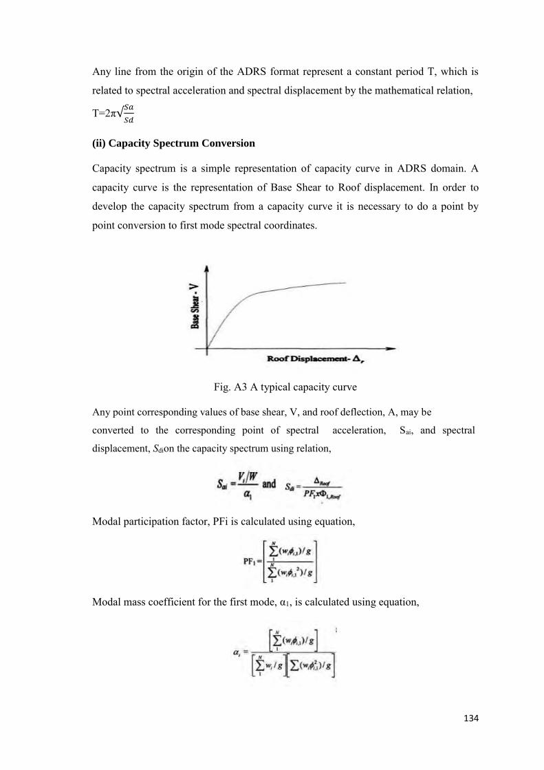
134

Any line from the origin of the ADRS format represent a constant period T, which is

related to spectral acceleration and spectral displacement by the mathematical relation,

T=2π√𝑆𝑎

𝑆𝑑

(ii) Capacity Spectrum Conversion

Capacity spectrum is a simple representation of capacity curve in ADRS domain. A

capacity curve is the representation of Base Shear to Roof displacement. In order to

develop the capacity spectrum from a capacity curve it is necessary to do a point by

point conversion to first mode spectral coordinates.

Fig. A3 A typical capacity curve

Any point corresponding values of base shear, V, and roof deflection, A, may be converted to the corresponding point of spectral acceleration, Sai, and spectral

displacement, Sdion the capacity spectrum using relation,

Modal participation factor, PFi is calculated using equation,

Modal mass coefficient for the first mode, α1, is calculated using equation,

135

Where: PF1 = Modal participation factor for the first natural mode. α1 = Modal mass coefficient for the first natural mode Φ1,Roof =Roof level amplitude of the first mode. Wi/g = Mass assigned to level i

φi,1 = Amplitude of mode 1 at level i N = Level N, the level which is the uppermost in the main portion of the structure V = Base shear W = Building dead weight plus likely live loads ∆Roof= Roof displacement Sa= Spectral acceleration Sd = Spectral displacement

Fig. A4 Capacity Spectrum

Fig. A.4 shows a typical capacity spectrum converted from capacity curve of Fig. C.3

of a hypothetical structure. It is seen in the capacity spectrum that up to some

displacement corresponding to point A, the period is constant T1. That is the structure is

behaving elastically. As the structure deflects more to point B, it goes to inelastic

deformation and its period lengthens to T2

When the capacity curve is plotted in Sa vs. Sd coordinates, radial lines drawn from the

origin of the plot through the curve at various spectral displacements have a slope (ω΄),

where, ω΄is the radial frequency of the effective (or secant) first-mode response of the

structure if pushed by an earthquake to that spectral displacement.

Using the relationship T΄=2𝜋

ω΄, it is possible to calculate, for each of these radial lines,

the effective period of the structure if it is pushed to a given spectral displacements.

Fig. A.5 is a capacity spectrum plot obtained from the capacity curve of a hypothetical

structure shown in Fig. 3.1 and plotted with the effective modal periods shown.

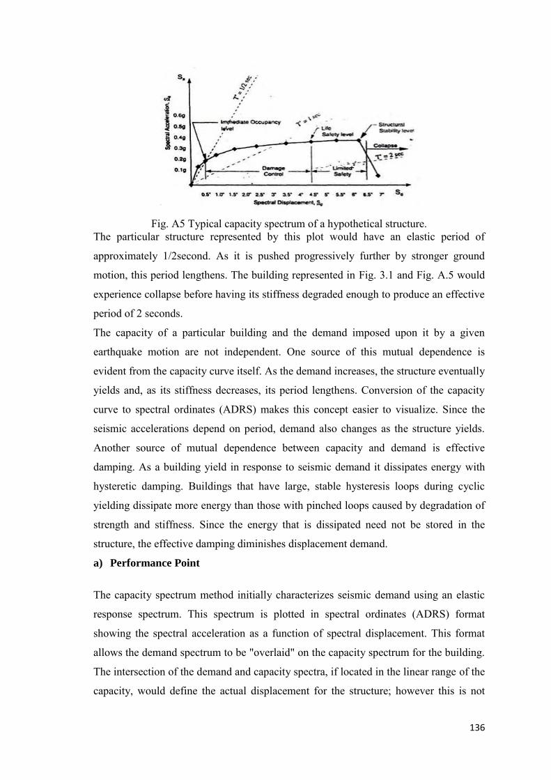
136

Fig. A5 Typical capacity spectrum of a hypothetical structure.

The particular structure represented by this plot would have an elastic period of

approximately 1/2second. As it is pushed progressively further by stronger ground

motion, this period lengthens. The building represented in Fig. 3.1 and Fig. A.5 would

experience collapse before having its stiffness degraded enough to produce an effective

period of 2 seconds.

The capacity of a particular building and the demand imposed upon it by a given

earthquake motion are not independent. One source of this mutual dependence is

evident from the capacity curve itself. As the demand increases, the structure eventually

yields and, as its stiffness decreases, its period lengthens. Conversion of the capacity

curve to spectral ordinates (ADRS) makes this concept easier to visualize. Since the

seismic accelerations depend on period, demand also changes as the structure yields.

Another source of mutual dependence between capacity and demand is effective

damping. As a building yield in response to seismic demand it dissipates energy with

hysteretic damping. Buildings that have large, stable hysteresis loops during cyclic

yielding dissipate more energy than those with pinched loops caused by degradation of

strength and stiffness. Since the energy that is dissipated need not be stored in the

structure, the effective damping diminishes displacement demand.

a) Performance Point

The capacity spectrum method initially characterizes seismic demand using an elastic

response spectrum. This spectrum is plotted in spectral ordinates (ADRS) format

showing the spectral acceleration as a function of spectral displacement. This format

allows the demand spectrum to be "overlaid" on the capacity spectrum for the building.

The intersection of the demand and capacity spectra, if located in the linear range of the

capacity, would define the actual displacement for the structure; however this is not

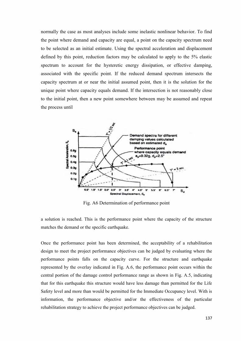
137

normally the case as most analyses include some inelastic nonlinear behavior. To find

the point where demand and capacity are equal, a point on the capacity spectrum need

to be selected as an initial estimate. Using the spectral acceleration and displacement

defined by this point, reduction factors may be calculated to apply to the 5% elastic

spectrum to account for the hysteretic energy dissipation, or effective damping,

associated with the specific point. If the reduced demand spectrum intersects the

capacity spectrum at or near the initial assumed point, then it is the solution for the

unique point where capacity equals demand. If the intersection is not reasonably close

to the initial point, then a new point somewhere between may be assumed and repeat

the process until

Fig. A6 Determination of performance point

a solution is reached. This is the performance point where the capacity of the structure

matches the demand or the specific earthquake.

Once the performance point has been determined, the acceptability of a rehabilitation

design to meet the project performance objectives can be judged by evaluating where the

performance points falls on the capacity curve. For the structure and earthquake

represented by the overlay indicated in Fig. A.6, the performance point occurs within the

central portion of the damage control performance range as shown in Fig. A.5, indicating

that for this earthquake this structure would have less damage than permitted for the Life

Safety level and more than would be permitted for the Immediate Occupancy level. With is

information, the performance objective and/or the effectiveness of the particular

rehabilitation strategy to achieve the project performance objectives can be judged.

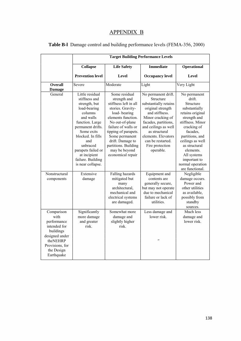
138

APPENDIX B

Table B-l Damage control and building performance levels (FEMA-356, 2000)

Target Building Performance Levels

Collapse Life Safety Immediate Operational

Prevention level Level Occupancy level Level

Overall Severe Moderate Light Very Light Damage General Little residual Some residual No permanent drift. No permanent

stiffness and strength and Structure drift. strength, but stiffness left in all substantially retains Structure load-bearing stories. Gravity- original strength substantially columns load- bearing and stiffness. retains original and walls elements function. Minor cracking of strength and function. Large No out-of-plane facades, partitions, stiffness. Minor permanent drifts. failure of walls or and ceilings as well cracking of Some exits tipping of parapets. as structural facades, blocked. In fills Some permanent elements. Elevators partitions, and and drift. Damage to can be restarted. ceilings as well unbraced partitions. Building Fire protection as structural parapets failed or may be beyond operable. elements. at incipient economical repair All systems failure. Building important to is near collapse. normal operation are functional.

Nonstructural Extensive Falling hazards Equipment and Negligible components damage mitigated but contents are damage occurs.

many generally secure, Power and architectural, but may not operate other utilities mechanical and due to mechanical as available, electrical systems failure or lack of possibly from are damaged. utilities. standby sources.

Comparison Significantly Somewhat more Less damage and Much less with more damage damage and lower risk. damage and

performance and greater slightly higher lower risk. intended for risk. risk.

buildings designed under

theNEHRP '' Provisions, for

the Design Earthquake

139

Table B-2 Structural performance levels and damagel,2,3 -Vertical Elements (FEMA-356, 2000)

Elements Structural Performance Levels

Type Collapse Prevention S-5 Life Safety S-3 Immediate Occupancy S-l

Primary Extensive cracking and hinge formation in ductile elements. Limited cracking and/or splice failure in some nqn-ductile columns. Severe damage in short columns.

Extensive damage to beams. Spalling of cover and shear cracking (<l/8" width) for ductile columns. Minor spalling in non-ductile columns. Joint cracks < 1/8" wide.

Minor hairline cracking. Limited yielding possible at a few locations. No crushing (strains below 0.003).

Secondary Extensive spalling in columns (limited shortening) and beams. Severe joint damage. Some reinforcing buckled.

Extensive cracking and hinge formation in ductile elements. Limited cracking and/or splice failure in some non ductile columns. Severe damage in short columns.

Minor spalling in non-ductile columns and beams. Flexural cracking in beams and columns. Shear cracking in joint width.

Drift 4% transient or permanent

2% transient; 1% permanent

1% transient; Negligible permanent

Steel Moment Frames

Primary Extensive distortion of beams and column panels. Many fractures at moment connections, but shear connections remain intact.

Hinges form. Local buckling of some beam elements. Severe joint distortion; isolated moment connection fractures, but shear connections remain intact. A few elements may experience partial fracture.

Minor or local yielding at a few places. No fractures. Minor buckling or observable permanent distortion of members.

Secondary Same as primary. Extensive distortion of beams and column panels. Many fractures at moment connections, but shear connections remain intact

Same as primary


2.5% transient; 1% permanent

0.7% transient; negligible permanent

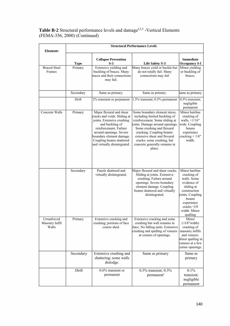
140

Table B-2 Structural performance levels and damagel,2,3 -Vertical Elements (FEMA-356, 2000) (Continued)

Elements

Structural Performance Levels

Type

Collapse Prevention

S-5 Life Safety S-3

Immediate

Occupancy S-l

Braced Steel Frames

Primary Extensive yielding and buckling of braces. Many

braces and their connections may fail.

Many braces yield or buckle but do not totally fail. Many

connections may fail

Minor yielding or buckling of

braces.

Secondary Same as primary. Same as primary. Same as primary.

Drift 2% transient or perjnanent 1.5% transient; 0.5% permanent 0.5% transient; negligible permanent

Concrete Walls Primary Major flexural and shear cracks and voids. Sliding at joints. Extensive crushing

and buckling of reinforcement. Failure

around openings. Severe boundary element damage. Coupling beams shattered and virtually disintegrated.

Some boundary element stress, including limited buckling of

reinforcement. Some sliding at joints. Damage around openings.

Some crushing and flexural cracking. Coupling beams: extensive shear and flexural cracks; some crushing, but

concrete generally remains in place.

Minor hairline cracking of

walls, <1/16" wide. Coupling

beams experience

cracking < 1/8" width.

Secondary Panels shattered and virtually disintegrated.

Major flexural and shear cracks. Sliding at joints. Extensive crushing, Failure around

openings. Severe boundary element damage. Coupling

beams shattered and virtually disintegrated.

Minor hairline cracking of walls. Some evidence of sliding at

construction joints. Coupling

beams experience cracks <l/8

width. Minor spalling

Urranfcrced Masonry Infill

Walls

Primary Extensive cracking and crushing; portions of face

course shed.

Extensive cracking and some crushing but wall remains in

place. No falling units. Extensive crushing and spalling of veneers

at corners of openings.

Minor (<l/8"width) cracking of

masonry infills and veneers.

Minor spalling in veneers at a few corner openings.

Secondary Extensive crushing and shattering; some walls

dislodge.

Same as primary Same as primary

Drift 0.6% transient or permanent

0.5% transient; 0.3% permanent'

0.1% transient; negligible permanent

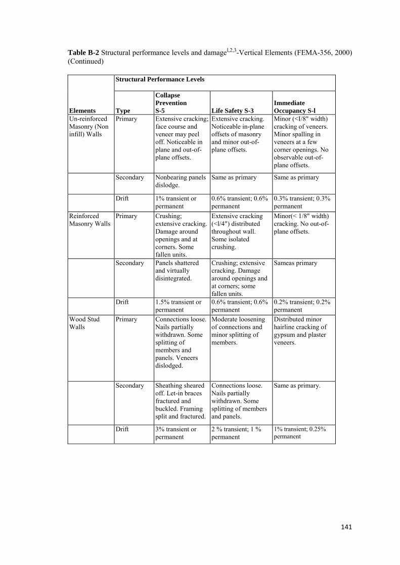
141

Table B-2 Structural performance levels and damagel,2,3-Vertical Elements (FEMA-356, 2000) (Continued)

Elements


Type

Collapse

Prevention S-5 Life Safety S-3

Immediate

Occupancy S-l Un-reinforced Masonry (Non infill) Walls

Primary Extensive cracking; face course and veneer may peel off. Noticeable in plane and out-of-plane offsets.

Extensive cracking. Noticeable in-plane offsets of masonry and minor out-of-plane offsets.

Minor (<I/8" width) cracking of veneers. Minor spalling in veneers at a few corner openings. No observable out-of-plane offsets.

Secondary Nonbearing panels dislodge.

Same as primary Same as primary


0.6% transient; 0.6% permanent


Reinforced Masonry Walls

Primary Crushing; extensive cracking. Damage around openings and at corners. Some fallen units.

Extensive cracking (<l/4") distributed throughout wall. Some isolated crushing.

Minor(< 1/8" width) cracking. No out-of-plane offsets.

Secondary Panels shattered and virtually disintegrated.

Crushing; extensive cracking. Damage around openings and at corners; some fallen units.

Sameas primary

Drift 1.5% transient or permanent



Wood Stud Walls

Primary Connections loose. Nails partially withdrawn. Some splitting of members and panels. Veneers dislodged.

Moderate loosening of connections and minor splitting of members.

Distributed minor hairline cracking of gypsum and plaster veneers.

Secondary Sheathing sheared off. Let-in braces fractured and buckled. Framing split and fractured.

Connections loose. Nails partially withdrawn. Some splitting of members and panels.

Same as primary.


2 % transient; 1 % permanent

1% transient; 0.25% permanent

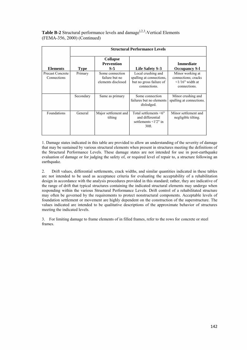
142

Table B-2 Structural performance levels and damagel,2,3-Vertical Elements (FEMA-356, 2000) (Continued)

Elements


Type

Collapse

Prevention

S-5 Life Safety S-3

Immediate

Occupancy S-l

Precast Concrete Connections

Primary Some connection failure but no

elements disclosed

Local crushing and spalling at connections, but no gross failure of

connections.

Minor working at connections; cracks

<1/16" width at connections.

Secondary Same as primary Some connection failures but no elements

dislodged.

Minor crushing and spalling at connections.

Foundations General Major settlement and tilting

Total settlements <6" and differential

settlements <1'2" in 30ft.

Minor settlement and negligible tilting.

1. Damage states indicated in this table are provided to allow an understanding of the severity of damage that may be sustained by various structural elements when present in structures meeting the definitions of the Structural Performance Levels. These damage states are not intended for use in post-earthquake evaluation of damage or for judging the safety of, or required level of repair to, a structure following an earthquake. 2. Drift values, differential settlements, crack widths, and similar quantities indicated in these tables arc not intended to be used as acceptance criteria for evaluating the acceptability of a rehabilitation design in accordance with the analysis procedures provided in this standard; rather, they are indicative of the range of drift that typical structures containing the indicated structural elements may undergo when responding within the various Structural Performance Levels. Drift control of a rehabilitated structure may often be governed by the requirements to protect nonstructural components. Acceptable levels of foundation settlement or movement are highly dependent on the construction of the superstructure. The values indicated are intended to be qualitative descriptions of the approximate behavior of structures meeting the indicated levels. 3. For limiting damage to frame elements of in filled frames, refer to the rows for concrete or steel frames.

143

Table B-3 Structural performance levels and damage1,2 - Horizontal elements (FEMA-356, 2000) Elements Structural Performance Levels

Collapse Prevention

S-5 Life Safety S-3

Immediate

Occupancy S-l

Metal Deck Diaphragms Large distortion with bucking of some units and tearing of many welds and seam attachments.

Some -localized failure of welded connections of deck to framing and between panels. Minor local bucking of deck.

Connections between deck units and framing intact. Minor distortions.

Wood Diaphragms Large permanent distortion with partial withdrawal of nails and extensive splitting of elements.

Some splitting at connections. Loosening of sheathing. Observable withdrawal of fasteners. Splitting and sheathing.

No observable loosening or withdrawal of fasteners. No splitting of sheathing or framing.

Concrete Diaphragms Extensive crushing and observable offset across many cracks.

Extensive cracking (<l/4"width). Local crushing and spalling.

Distributed hairline cracking. Some minor cracks of larger size (<l/8" width)

Precast Diaphragms Connections between units fail. Units shift relative to each other. Crushing and spalling at joints.

Extensive cracking (<l/4" width). Local crushing and spalling.

Some minor cracking along joints.

1. Damage states indicated in this table are provided to allow an understanding of the seventy of damage that may be sustained by various structural elements when present in structures meeting the definitions of the Structural Performance Levels. These damage states are not intended for use in post-earthquake evaluation of damage or for judging the safety of, or required level of repair to, a structure following an earthquake. 2. Drift values, differential settlements, crack widths, and similar quantities indicated in these tables are not intended to be used as acceptance criteria for evaluating the acceptability of a rehabilitation design in accordance with the analysis procedures provided in this standard; rather, they are indicative of the range of drift that typical structures containing the indicated structural elements may undergo when responding within the various Structural Performance Levels. Drifts control of a rehabilitated structure may often be governed by the requirements to protect nonstructural components. Acceptable levels of foundation settlement or movement are highly dependent on the construction of the superstructure. The values indicated are intended to be qualitative descriptions of the approximate behavior of structures meeting the indicated levels. Table B-4 Deformation Limits (ATC-40, 1996) Performance Level

Inter- story Drift Limit Immediate Occupancy

Damage Control

Life Safety Structural Stability

Maximum total drift 0.01 0.01 -0.02 0.02 0.33𝑉𝑖

𝑃𝑖

Maximum inelastic drift 0.005 0.005-0.015 No limit No limit

144

Table B-5 Examples of Possible Deformation-Controlled and Force-Controlled Actions(FEMA-356, 2000)

Component Deformation-

Controlled Action Force-Controlled Action

Moment Frames Beam Columns Moment (M) M Shear (V) Axial load (P), V Joints - V1 Shear Walls M, V P Braced Frames Braces P — Beams — P Columns — P Shear Link V P, M

Connections P, V, M3 P, V, M

Diaphragms M,V2 P, V, M

1. Shear may be a deformation-controlled action in steel moment frame connection 2. If the diaphragm carries lateral loads from vertical seismic resisting elements above the

diaphragm level, then M and V shall be considered force-controlled actions. 3. Axial, shear, and moment may be deformation-controlled actions for certain steel and wood

connections. Table B-6 Numerical Acceptance Criteria for Plastic Hinge Rotations in Reinforced Concrete Beams, in radians (ATC-40, 1996) Performance Level3

Primary Secondary Component Type IO LS SS LS SS 1. Beams Controlled by Flexure1

𝜌 − 𝜌′

𝜌𝑏𝑎𝑙

Transverse Reinforcement2 𝑉4

𝑏𝑤𝑑 √𝑓′𝑐

≤0.0 C ≤3 0.005 0.020 0.025 0.020 0.050 ≤0.0 C ≥6 0.005 0.010 0.020 0.020 0.040 ≥0.5 C ≤3 0.005 0.010 0.020 0.020 0.030 ≥0.5 C ≥6 0.005 0.005 0.015 0.015 0.020 ≤0.0 NC ≤3 0.005 0.010 0.020 0.020 0.030 ≤0.0 NC ≥6 0.000 0.005 0.010 0.010 0.015 ≥0.5 NC ≤3 0.005 0.010 0.010 0.010 0.015 ≥0.5 NC ≥6 0.000 0.005 0.005 0.005 0.010 2. Beams controlled by shear1 Stirrup spacing ≤ d/2 0.0 0.0 0.0 0.010 0.02 Stirrup spacing > d/2 0.0 0.0 0.0 0.005 0.01 3. Beams controlled by inadequate development or splicing along the span1 Stirrup spacing ≤d/2 0.0 0.0 0.0 0.010 0.02 Stirrup spacing > d/2 0.0 0.0 0.0 0.005 0.01 4. Beams controlled by inadequate embedment into beam-column joint1 0.0 0.01 0.015 0.02 0.03

145

1. When more than one of the conditions 1.2.3 and 4 occur for a given component, use the minimum appropriate numerical value from the table. 2. Under the heading "transverse reinforcement." 'C' and 'NC' are abbreviations for conforming and non-conforming details, respectively. A component is conforming if within the flexural plastic region: (1) closed stirrup are spaced at <d/3 and 2) for components of moderate and high ductility demand the strength provided by the stirrup (Vs) is at least three-fourths of the design shear. Otherwise,component is considered non-conforming. 3. Linear interpolation between values listed in the table is permitted.

IO = Immediate Occupancy LS = Life Safety SS = Structural Stability. 4. V = Design Shear Table B-7 Numerical Acceptance Criteria for Plastic Hinge Rotations in Reinforced ' Concrete Columns, in radians (ATC-40, 1996) Performance Level4

Primary Secondary Component Type IO LS SS LS SS 1. Columns Controlled by Flexure1

𝑃5

𝐴𝑔𝑓′𝑐

Transverse Reinforcement2

𝑉4


≤0.1 C ≤3 0.005 0.010 0.020 0.015 0.030 ≤0.1 C ≥6 0.005 0.010 0.015 0.010 0.025 ≥0.4 C ≤3 0.000 0.005 0.015 0.010 0.025 ≥0.4 C ≥6 0.000 0.005 0.010 0.010 0.015 ≤0.1 NC ≤3 0.005 0.005 0.010 0.005 0.015 ≤0.1 NC ≥6 0.005 0.005 0.005 0.005 0.005 ≥0.4 NC ≤3 0.000 0.000 0.005 0.000 0.005 ≥0.4 NC ≥6 0.000 0.000 0.000 0.000 0.000 2. Columns controlled by shear1"3 Hoop Spacing

≤ d/2 Or

𝑃5

𝐴𝑔𝑓′𝑐

0.000 0.000 0.000 0.01 0.015

Other cases 0.000 0.000 0.000 0.00 0.000 3. Columns controlled by inadequate development or splicing along the clear height1"3 Hoop spacing <d/2 0.0 0.0 0.0 0.01 0.02 Hoop spacing >d/2 0.0 0.0 0.0 0.005 0.01 4. Columns with axial loads exceeding 0.70 '** Conforming reinforcement over

the entire length 0.0 0.0 0.005 0.005 0.01

All other cases 0.0 0.0 0.0 0.0 0.0

1. When more than one of the conditions 1.2.3 and 4 occur for a given component, use the minimum appropriate numerical value from the table. See Chapter 9 for symbol definitions.

2. Under the heading "transverse reinforcement." "C' and 'NC' are abbreviations for conforming and non-conforming details, respectively. A component is conforming if within the flexural plastic hinge region: (1) closed hoops are spaced at <d/3 and 2) for components of moderate and high ductility demand the strength provided by the stirrup (Vs) is at least three-fourths of the design shear. Otherwise, the component is considered non-conforming

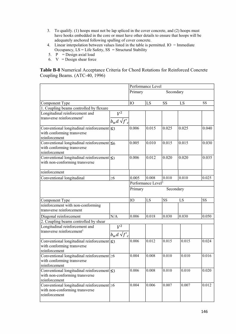
146

3. To qualify. (1) hoops must not be lap spliced in the cover concrete, and (2) hoops must have hooks embedded in the core or must have other details to ensure that hoops will be adequately anchored following spalling of cover concrete.

4. Linear interpolation between values listed in the table is permitted. IO = Immediate Occupancy, LS = Life Safety, SS = Structural Stability

5. P = Design axial load 6. V = Design shear force Table B-8 Numerical Acceptance Criteria for Chord Rotations for Reinforced Concrete Coupling Beams. (ATC-40, 1996) _ Performance Level

Primary Secondary

Component Type IO LS SS LS SS 1. Coupling beams controlled by flexure Longitudinal reinforcement and transverse reinforcement1

𝑉2


Conventional longitudinal reinforcement with conforming transverse reinforcement

≤3 0.006 0.015 0.025 0.025 0.040


≤6 0.005 0.010 0.015 0.015 0.030

Conventional longitudinal reinforcement with non-conforming transverse

≤3 0.006 0.012 0.020 0.020 0.035

reinforcement Conventional longitudinal ≥6 0.005 0.008 0.010 0.010 0.025 Performance Level3

Primary Secondary

Component Type IO LS SS LS SS reinforcement with non-conforming transverse reinforcement

Diagonal reinforcement N/A 0.006 0.018 0.030 0.030 0.050 2. Coupling beams controlled by shear Longitudinal reinforcement and transverse reinforcement1

𝑉2



≤3 0.006 0.012 0.015 0.015 0.024


≥6 0.004 0.008 0.010 0.010 0.016

Conventional longitudinal reinforcement with non-conforming transverse reinforcement

≤3 0.006 0.008 0.010 0.010 0.020

Conventional longitudinal reinforcement with non-conforming transverse reinforcement

≥6 0.004 0.006 0.007 0.007 0.012

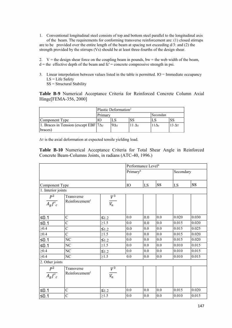
147

1. Conventional longitudinal steel consists of top and bottom steel parallel to the longitudinal axis of the beam. The requirements for conforming transverse reinforcement are: (1) closed stirrups are to be provided over the entire length of the beam at spacing not exceeding d/3: and (2) the strength provided by the stirrups (Vs) should be at least three-fourths of the design shear. 2. V = the design shear force on the coupling beam in pounds, bw = the web width of the beam, d = the effective depth of the beam and fc' = concrete compressive strength in psi. 3. Linear interpolation between values listed in the table is permitted. IO = Immediate occupancy LS = Life Safety SS = Structural Stability Table B-9 Numerical Acceptance Criteria for Reinforced Concrete Column Axial Hinge[FEMA-356, 2000] Plastic Deformation1

Primary Secondan Component Type IO LS SS LS SS 1. Braces in Tension (except EBF braces)

7∆T 9∆T 11 ∆T 11∆T 13 ∆T

∆T is the axial deformation at expected tensile yielding load. Table B-10 Numerical Acceptance Criteria for Total Shear Angle in Reinforced Concrete Beam-Columns Joints, in radians (ATC-40, 1996.) Performance Level4

Primary6 Secondary

Component Type IO LS ss LS ss 1. Interior joints

𝑃2

𝐴𝑔𝑓′𝑐


𝑉3

𝑉𝑛

≤0.1 C ≤1.2 0.0 0.0 0.0 0.020 0.030 ≤0.1 C ≥1.5 0.0 0.0 0.0 0.015 0.020 ≥0.4 C ≤1.2 0.0 0.0 0.0 0.015 0.025 ≥0.4 C ≥1.5 0.0 0.0 0.0 0.015 0.020 ≤0.1 NC ≤1.2 0.0 0.0 0.0 0.015 0.020 ≤0.1 NC ≥1.5 0.0 0.0 0.0 0.010 0.015 ≥0.4 NC ≤1.2 0.0 0.0 0.0 0.010 0.015 ≥0.4 NC ≥1.5 0.0 0.0 0.0 0.010 0.015 2. Other joints

𝑃2

𝐴𝑔𝑓′𝑐


𝑉3

𝑉𝑛

≤0.1 C ≤1.2 0.0 0.0 0.0 0.015 0.020 ≤0.1 C ≥1.5 0.0 0.0 0.0 0.010 0.015

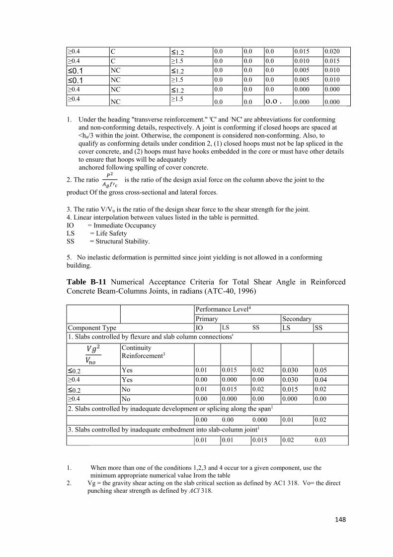
148

≥0.4 C ≤1.2 0.0 0.0 0.0 0.015 0.020 ≥0.4 C ≥1.5 0.0 0.0 0.0 0.010 0.015 ≤0.1 NC ≤1.2 0.0 0.0 0.0 0.005 0.010 ≤0.1 NC ≥1.5 0.0 0.0 0.0 0.005 0.010 ≥0.4 NC ≤1.2 0.0 0.0 0.0 0.000 0.000 ≥0.4 NC ≥1.5 0.0 0.0 o.o . 0.000 0.000 1. Under the heading "transverse reinforcement." 'C' and :NC' are abbreviations for conforming

and non-conforming details, respectively. A joint is conforming if closed hoops are spaced at <hu/3 within the joint. Otherwise, the component is considered non-conforming. Also, to qualify as conforming details under condition 2, (1) closed hoops must not be lap spliced in the cover concrete, and (2) hoops must have hooks embedded in the core or must have other details to ensure that hoops will be adequately

anchored following spalling of cover concrete.

2. The ratio 𝑃2

𝐴𝑔𝑓′𝑐 is the ratio of the design axial force on the column above the joint to the

product Of the gross cross-sectional and lateral forces. 3. The ratio V/Vn is the ratio of the design shear force to the shear strength for the joint. 4. Linear interpolation between values listed in the table is permitted. IO = Immediate Occupancy LS = Life Safety SS = Structural Stability. 5. No inelastic deformation is permitted since joint yielding is not allowed in a conforming building. Table B-11 Numerical Acceptance Criteria for Total Shear Angle in Reinforced Concrete Beam-Columns Joints, in radians (ATC-40, 1996) Performance Level4

Primary Secondary Component Type IO LS SS LS SS 1. Slabs controlled by flexure and slab column connections'

𝑉𝑔2

𝑉𝑛𝑜

Continuity Reinforcement3

≤0.2 Yes 0.01 0.015 0.02 0.030 0.05 ≥0.4 Yes 0.00 0.000 0.00 0.030 0.04 ≤0.2 No 0.01 0.015 0.02 0.015 0.02 ≥0.4 No 0.00 0.000 0.00 0.000 0.00 2. Slabs controlled by inadequate development or splicing along the span1 0.00 0.00 0.000 0.01 0.02 3. Slabs controlled by inadequate embedment into slab-column joint1 0.01 0.01 0.015 0.02 0.03

1. When more than one of the conditions 1,2,3 and 4 occur tor a given component, use the minimum appropriate numerical value Irom the table

2. Vg = the gravity shear acting on the slab critical section as defined by AC1 318. Vo= the direct punching shear strength as defined by ACl 318.

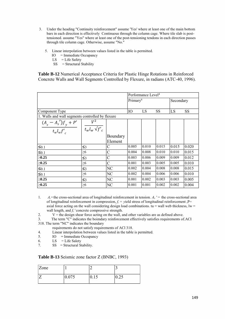
149

3. Under the heading "Continuity reinforcement" assume 'Yes' where at least one of the main bottom bars in each direction is effectively Continuous through the column cage. Where tile slab is post- tensioned. assume "Yes" where at least one of the post-tensioning tendons in each direction passes through tile column cage. Otherwise, assume "No."

5. Linear interpolation between values listed in the table is permitted. IO = Immediate Occupancy

LS = Life Safety SS = Structural Stability Table B-12 Numerical Acceptance Criteria for Plastic Hinge Rotations in Reinforced Concrete Walls and Wall Segments Controlled by Flexure, in radians (ATC-40, 1996).

1. A,=the cross-sectional area of longitudinal reinforcement in tension. As ' = the cross-sectional area of longitudinal reinforcement in compression, f, = yield stress of longitudinal reinforcement ,P= axial force acting on the wall considering design load combinations. tu = wall web thickness, lw = wall length, and fc’:concrete compressive strength. 2. V = the design shear force acting on the wall, and other variables are as defined above. 3. The term "C" indicates the boimdary reinforcement effectively satisfies requirements of.ACI 318. The term "NC" indicates the boundary requirements do not satisfy requirements of ACl 318. 4. Linear interpolation between values listed in the table is permitted. 5. IO = Immediate Occupancy 6. LS = Life Salety 7. SS = Structural Stability. Table B-13 Seismic zone factor Z (BNBC, 1993) Zone 1 2 3

Z 0.075 0.15 0.25

Performance Level4

Primary6 Secondary

Component Type IO LS SS LS SS 1. Walls and wall segments controlled by flexure

(𝐴𝑠

− 𝐴𝑠′)𝑓𝑦

+ 𝑃′

𝑡𝑤𝑙𝑤𝑓′𝑐

𝑉2

𝑡𝑤𝑙𝑤 √𝑓′𝑐

Boundary Element

≤0.1 ≤3 C 0.005 0.010 0.015 0.015 0.020 ≤0.1 ≥6 C 0.004 0.008 0.010 0.010 0.015 ≥0.25 ≤3 C 0.003 0.006 0.009 0.009 0.012 ≥0.25 ≥6 C 0.001 0.003 0.005 0.005 0.010 ≤0.1 ≤3 NC 0.002 0.004 0.008 0.008 0.015 ≤0.1 ≥6 NC 0.002 0.004 0.006 0.006 0.010 ≥0.25 ≤3 NC 0.001 0.002 0.003 0.003 0.005 ≥0.25 ≥6 NC 0.001 0.001 0.002 0.002 0.004

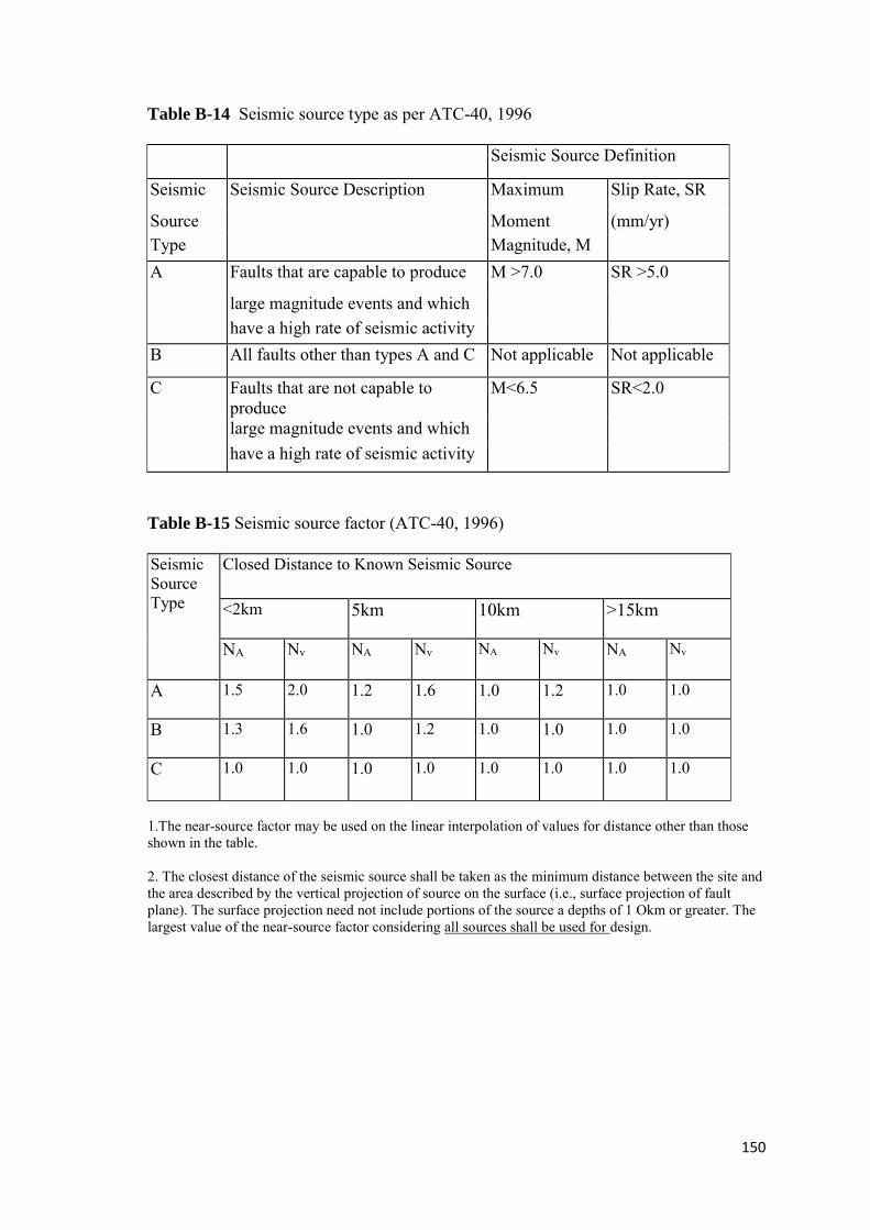
150

Table B-14 Seismic source type as per ATC-40, 1996 Seismic Source Definition

Seismic Seismic Source Description Maximum Slip Rate, SR

Source Moment (mm/yr) Type Magnitude, M A Faults that are capable to produce M >7.0 SR >5.0

large magnitude events and which have a high rate of seismic activity B All faults other than types A and C Not applicable Not applicable

C Faults that are not capable to produce

M<6.5 SR<2.0

large magnitude events and which have a high rate of seismic activity

Table B-15 Seismic source factor (ATC-40, 1996) Seismic Source Type

Closed Distance to Known Seismic Source

<2km 5km 10km >15km

NA Nv NA Nv NA Nv NA Nv

A 1.5 2.0 1.2 1.6 1.0 1.2 1.0 1.0

B 1.3 1.6 1.0 1.2 1.0 1.0 1.0 1.0

C 1.0 1.0 1.0 1.0 1.0 1.0 1.0 1.0

1.The near-source factor may be used on the linear interpolation of values for distance other than those shown in the table. 2. The closest distance of the seismic source shall be taken as the minimum distance between the site and the area described by the vertical projection of source on the surface (i.e., surface projection of fault plane). The surface projection need not include portions of the source a depths of 1 Okm or greater. The largest value of the near-source factor considering all sources shall be used for design.

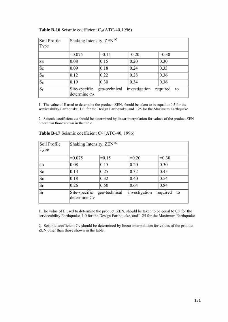
151

Table B-16 Seismic coefficient CA(ATC-40,1996) Soil Profile Type

Shaking Intensity, ZEN1'2

=0.075 =0.15 -0.20 =0.30 SB 0.08 0.15 0.20 0.30 Sc 0.09 0.18 0.24 0.33 SD 0.12 0.22 0.28 0.36 SE 0.19 0.30 0.34 0.36 SF Site-specific geo-technical investigation required to

determine CA 1. The value of E used to determine the product, ZEN, should be taken to be equal to 0.5 for the serviceability Earthquake, 1.0. for the Design Earthquake, and 1.25 for the Maximum Earthquake. 2. Seismic coefficient CA should be determined by linear interpolation for values of the product ZEN other than those shown in the table. Table B-17 Seismic coefficient Cv (ATC-40, 1996) Soil Profile Type

Shaking Intensity, ZEN1'2

=0.075 =0.15 =0.20 =0.30 SB 0.08 0.15 0.20 0.30 Sc 0.13 0.25 0.32 0.45 So 0.18 0.32 0.40 0.54 SE 0.26 0.50 0.64 0.84 SF Site-specific geo-technical investigation required to

determine Cv

1.The value of E used to determine the product, ZEN, should be taken to be equal to 0.5 for the serviceability Earthquake, 1.0 for the Design Earthquake, and 1.25 for the Maximum Earthquake.

2. Seismic coefficient Cv should be determined by linear interpolation for values of the product ZEN other than those shown in the table.

152

Table B-18 Soil profile types (ATC-40, 1996) Average Soil Properties for Top 100 ft of Soil Profile

Soil Soil Profile Share Wave Standard Undrained Shear

Profile Name/ Velocity, Vs (ft/sec) Penetration Test, Strength, Su Type Generic N or Ncn for (psf) Description cohesion less soil layers (blow/ft) SA Hard Rock Vs>5,000 Not Applicable

SB Rock 2,500 < Vs< 5,000 Not Applicable SC Very Dense 1,200 <VS< 2,500 N>50 N>50 Soil and Rock SD Stiff Soil 600 <VS< 1,200 15 < N < 50 1,000<SU Profile < 2,000 SE Soft Soil Vs< 600 N<50 Su< 1,000 Profile SF Soil Require Site-Specific Evaluation

Soil profile SA is not applicable to site in Dhaka. For the purpose of the analysis of the structures considered in this thesis soil type SD has been considered.

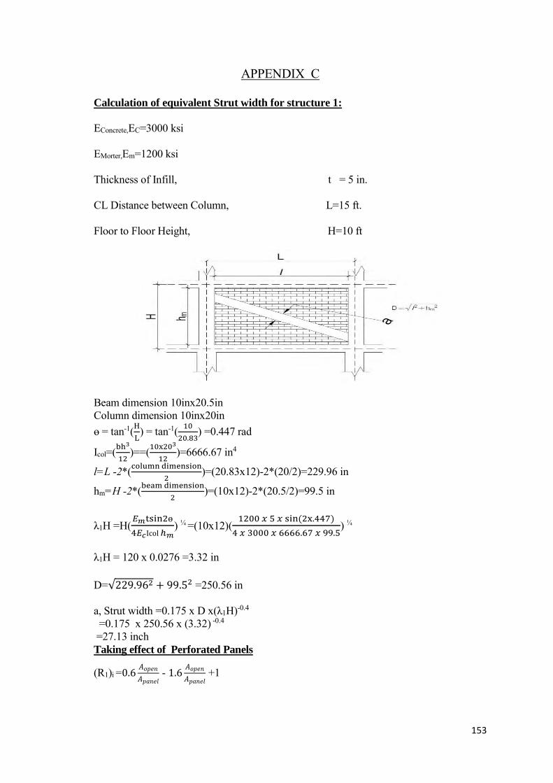
153

APPENDIX C

Calculation of equivalent Strut width for structure 1:

EConcrete,EC=3000 ksi EMorter,Em=1200 ksi Thickness of Infill, t = 5 in. CL Distance between Column, L=15 ft. Floor to Floor Height, H=10 ft

Beam dimension 10inx20.5in Column dimension 10inx20in ɵ = tan-1(H

L) = tan-1( 10

20.83) =0.447 rad

Icol=(bh3

12)==(10x203

12)=6666.67 in4

l=L -2*(column dimension

2)=(20.83x12)-2*(20/2)=229.96 in

hm=H -2*(beam dimension

2)=(10x12)-2*(20.5/2)=99.5 in

λ1H =H(𝐸𝑚tsin2ɵ

4𝐸𝑐Icol ℎ𝑚) ¼ =(10x12)(

1200 𝑥 5 𝑥 sin (2x.447)

4 𝑥 3000 𝑥 6666.67 𝑥 99.5) ¼

λ1H = 120 x 0.0276 =3.32 in D=√229.962 + 99.52 =250.56 in a, Strut width =0.175 x D x(λ1H)-0.4

=0.175 x 250.56 x (3.32) -0.4 =27.13 inch Taking effect of Perforated Panels

(R1)i =0.6𝐴𝑜𝑝𝑒𝑛

𝐴𝑝𝑎𝑛𝑒𝑙 - 1.6

𝐴𝑜𝑝𝑒𝑛

𝐴𝑝𝑎𝑛𝑒𝑙 +1

154

Where: Aopen= Area of the opening (in2)


Note: If the area of the opening (A open) is greater than or equal to 60 percent of the infill panel (Apanel) then the effect of the infill should be neglected.

Aopen=5 ft x 4.5ft x12x12 =3240 in2

Apanel=l x hm =229.96 x 99.5=22881.02 in2

( 𝐴𝑜𝑝𝑒𝑛

𝐴𝑝𝑎𝑛𝑒𝑙)= ( 3240

22881.02)=0.1416

(R1)i=0.6 x 0.1416 –(1.6 x 0.1416)+1=0.8584=0.86 Modified strut width for perforated panel = 0.86 x 27.13 in =23.05 inch.

tan (ɵcolumn)=(ℎ𝑚−

a

cos (ɵcolumn))

𝑙)

For, ɵcolumn = 0.45 radian

tan (0.45)=(99.5−

27.13

cos (0.45))

229.96)

= 0.30 Assuming ɵcolumn = 0.30 radian lcolumn =( a

cos (ɵcolumn)= ( 27.13

cos (0.3))

= 28.39 inch ≅ 29 inch Calculation of equivalent Strut width for structure 2:

EConcrete,EC=3000 ksi EMorter,Em=1200 ksi Thickness of Infill, t = 5 in. CL Distance between Column, L=12.83 ft. Floor to Floor Height, H=10 ft

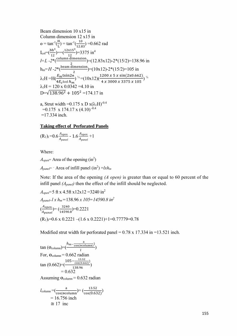
155

Beam dimension 10 x15 in Column dimension 12 x15 in ɵ = tan-1(H

L) = tan-1( 10

12.83) =0.662 rad

Icol=(bh3

12)==(12x153

12)=3375 in4

l=L -2*(column dimension

2)=(12.83x12)-2*(15/2)=138.96 in

hm=H -2*(beam dimension

2)=(10x12)-2*(15/2)=105 in

λ1H =H(𝐸𝑚tsin2ɵ

4𝐸𝑐Icol ℎ𝑚) ¼ =(10x12)(

1200 𝑥 5 𝑥 sin (2x0.662)

4 𝑥 3000 𝑥 3375 𝑥 105) ¼

λ1H = 120 x 0.0342 =4.10 in D=√138.962 + 1052 =174.17 in a, Strut width =0.175 x D x(λ1H)-0.4

=0.175 x 174.17 x (4.10) -0.4 =17.334 inch. Taking effect of Perforated Panels

(R1)i =0.6𝐴𝑜𝑝𝑒𝑛

𝐴𝑝𝑎𝑛𝑒𝑙 - 1.6

𝐴𝑜𝑝𝑒𝑛

𝐴𝑝𝑎𝑛𝑒𝑙 +1

Where:

Aopen= Area of the opening (in2)


Note: If the area of the opening (A open) is greater than or equal to 60 percent of the infill panel (Apanel) then the effect of the infill should be neglected.

Aopen=5 ft x 4.5ft x12x12 =3240 in2

Apanel=l x hm =138.96 x 105=14590.8 in2

( 𝐴𝑜𝑝𝑒𝑛

𝐴𝑝𝑎𝑛𝑒𝑙)= ( 3240

14590.8)=0.2221

(R1)i=0.6 x 0.2221 –(1.6 x 0.2221)+1=0.77779=0.78 Modified strut width for perforated panel = 0.78 x 17.334 in =13.521 inch.

tan (ɵcolumn)=(ℎ𝑚−

a

cos (ɵcolumn))

𝑙)

For, ɵcolumn = 0.662 radian

tan (0.662)=(105−

13.52

cos (0.662))

138.96)

= 0.632 Assuming ɵcolumn = 0.632 radian lcolumn =( a

cos (ɵcolumn)= ( 13.52

cos (0.632))

= 16.756 inch ≅ 17 inc

seismic performance evaluation of different …

Documents