seismic modeling engines phase 1from north america will come from land reservoirs. if geophysics is...

DOE/ER/86230-1

SEISMIC MODELING ENGINES PHASE 1

PHASE 1 FINAL REPORT, PROJECT PERIOD SEPTEMBER 2005 – APRIL 2005

FEBRUARY 2006

BRUCE P. MARION

Z-SEIS CORPORATION HOUSTON, TEXAS

DISTRIBUTION A –APPROVED FOR PUBLIC RELEASE; FURTHER DISSEMINATION UNLIMITED.

DOE/ER/86230-1

SEISMIC MODELING ENGINES

PHASE 1

FINAL REPORT FOR THE PROJECT PERIOD SEPTEMBER 2004 – APRIL 2005

DATE ISSUED/PUBLISHED FEBRUARY 2006

BRUCE P. MARION

PREPARED FOR THE UNITED STATES

DEPARTMENT OF ENERGY

WORK PERFORMED UNDER CONTRACT NO. DE-FG02-04ER86230

PHASE 1 FINAL REPORT — DE-FG02-04ER86230 PAGE i

TABLE OF CONTENTS

Abstract........................................................................................................................................... 1

Introduction and Summary ........................................................................................................... 2 Identification and significance of the problem....................................................................... 2 Technical approach................................................................................................................... 5

Anticipated Benefits ....................................................................................................................... 5 General benefits to the industry .............................................................................................. 5 Specific benefits to the industry............................................................................................... 6

Accomplishment of Phase I Objectives ......................................................................................... 7 Background ............................................................................................................................... 7

Seismic Modeling Engines ..................................................................................................... 7 Isotropic acoustic wave equation............................................................................................. 8 Isotropic elastic wave equation................................................................................................ 9 Anisotropic acoustic wave equation ...................................................................................... 10 Anisotropic elastic wave equation ......................................................................................... 11 Eikonal ray tracing ................................................................................................................. 12 Additions to the existing codes............................................................................................... 13

A) Variable gridding for both vertical and horizontal directions.......................................... 13 B) Attenuation incorporated (intrinsic constant Q)............................................................... 15 C) Perfectly matched layer (PML) absorbing boundary conditions ..................................... 16 D) Optimal coefficient finite difference................................................................................ 17

Testing...................................................................................................................................... 19 Timing tests........................................................................................................................... 19

Examples.................................................................................................................................. 19

Conclusions and Recommendations ........................................................................................... 25 Technical Objectives for Future Work................................................................................. 25 Detailed Work Plan for Future Technical Work................................................................. 26

Thin layer dynamic equivalent media................................................................................... 26 Finalize modeling engines .................................................................................................... 27 Arbitrary source and receiver positions ................................................................................ 27 Source types and wavelets .................................................................................................... 28 1. Source ............................................................................................................................... 28 2. Fractures............................................................................................................................ 28 Lateral heterogeneity ............................................................................................................ 29

Technical references .................................................................................................................... 30

PHASE 1 FINAL REPORT — DE-FG02-04ER86230 PAGE 1

Abstract Seismic modeling is a core component of petroleum exploration and production today. Potential applications include modeling the influence of dip on anisotropic migration; source/receiver placement in deviated-well three-dimensional surveys for vertical seismic profiling (VSP); and the generation of realistic data sets for testing contractor-supplied migration algorithms or for interpreting AVO (amplitude variation with offset) responses.

This project was designed to extend the use of a finite-difference modeling package, developed at Lawrence Berkeley Laboratories, to the advanced applications needed by industry. The approach included a realistic, easy-to-use 2-D modeling package for the desktop of the practicing geophysicist.

The feasibility of providing a wide-ranging set of seismic modeling engines was fully demonstrated in Phase I. The technical focus was on adding variable gridding in both the horizontal and vertical directions, incorporating attenuation, improving absorbing boundary conditions and adding the optional coefficient finite difference methods.


Introduction and Summary

Identification and significance of the problem As geoscientists become more involved in the characterization of the reservoir, the use of seismic attributes and amplitudes to measure reservoir properties such as porosity, pressure, saturation, and, ultimately, perhaps permeability is becoming commonplace. Understanding not only the traveltimes of seismic waves, but also their local amplitude and phase characteristics is more important for reservoir characterization applications than for rank exploration. In many software packages, there are tools to create synthetic seismograms from well logs and tools to relate these synthetic seismograms to important reservoir properties. These tools are typically idealized representations of the seismic reflection survey. They do not capture important characteristics such as short wavelength heterogeneity, Q, anisotropy, local wavefront curvature, etc, that may affect the relationship between the reservoir properties of interest and the real seismic data. To create the link between reservoir properties and the details of the seismic wavefield requires much more realistic synthetic seismograms, which, in turn, necessitates more realistic seismic modeling tools to create these synthetic seismograms. Finite difference (FD) modeling is a well-characterized and efficient tool for creating these more sophisticated synthetic seismograms. FD modeling can also be used in more conventional applications such as illumination studies, acquisition planning, and migration testing.

Seismic modeling forms a core component of most endeavors in petroleum exploration and production today. The use of seismic modeling spans applications ranging from modeling the influence of dip on anisotropic migration to illumination studies and source/receiver placement in deviated-well 3-D VSP surveys. Other applications include generation of realistic data sets for testing of contractor-supplied migration algorithms, or for interpreting AVO responses. With the recent advances in reverse-time migration, seismic modeling engines can also be used to implement migration.

The general need is for realistic seismic modeling of the important properties and processes governing seismic wave propagation in the earth. Realistic carries different meanings for the range of geophysical applications depending on rock properties that are dominating the seismic response. For example, in the exploration/production context, realistic can mean the ability to model wave kinematics on the scale of 20 km3 at frequencies up to 50 Hz while accommodating the large velocity-density contrasts encountered in subsalt applications. In these cases, 3-D anisotropic acoustic modeling may be adequate. In other applications, such as AVO and time-lapse seismic, amplitudes are critical and accurate simulation of elastic wave propagation and attenuation may be required.

Modeling has essential utility for testing of imaging and processing algorithms with ground truth in the form of known models. Specific areas of application include:

• Migration techniques • AVO inversion • Parameter sensitivity especially in time-lapse seismic Another important use for modeling is in illumination studies and survey design. Parameters such as shot and receiver density and placement and maximum offset can be analyzed. Complex structure can be incorporated such as 3-D surface seismic subsalt imaging. Novel geometries especially for sub-surface seismology can be modeled, including:


• 3-D VSP • Deviated wellbore borehole surveys • Horizontal well borehole surveys • Ocean Bottom Cable (OBC) recording • Crosswell seismic. As an example, consider an anisotropic migration algorithm. The sample model is shown in Figure 1 with the anisotropy axis of symmetry perpendicular to the bedding. Examples of shot gathers for both a VTI and TTI assumption are shown in Figure 2. When the model of Figure 1 is imaged with a vertical axis of symmetry, the true structure is mispositioned as shown in Figure 3. Figure 4 shows the improvement of using the true model with a tilted axis of symmetry for the anisotropy assumption. Modeling is an excellent means of determining the impact of simplifying assumptions in imaging methods.

Figure 1. Model for anisotropic migration example.

Distance (m)

Dep

th ( m

)

P-wave Velocity (m/s)Distance (m)

Dep

th ( m

)

P-wave Velocity (m/s)


Figure 2. Example shot gathers for VTI and TTI assumption.

Figure 3. Migration with vertical axis of symmetry. True structure shown in red.

VTI TTIVTI TTI


Figure 4. Migration with tilted axis of symmetry. True structure shown in red.

Technical approach The models shown in the example above were generated with a finite-difference modeling package developed at Lawrence Berkeley Laboratories. Basic 2-D and 3-D serial and parallel codes have been developed and have been widely tested and applied in a variety of applications, structural assumptions and source/receiver geometries. The overall objective of the planned three-phase project was to commercialize the modeling code of LBL and extend it to industry-needed advanced applications. In Phase I we addressed some remaining research and feasibility issues in concert with the original developers from LBL. What remains for the future includes adding several features to the basic modeling code. A user-friendly interface tapping the GEM graphics-based earth modeling software from LBL also needs to be developed. The targeted commercialization strategy should include any or all of: (1) an easy-to-use 2-D desktop package for practicing geophysicists, (2) a parallelized 3-D package and (3) a modeling service offering to the industry. In parallel with these efforts, a consortium of industry users should be established including major E&P companies to guide and mentor the development and serve as the basis for an ongoing users group to be involved in initial testing and evaluation.

Anticipated Benefits

General benefits to the industry The role of geophysics is slowly transitioning to reservoir applications. Although many geophysicists are still focused on offshore and exploration opportunities, secure energy supplies from North America will come from land reservoirs. If geophysics is to maintain an ongoing role in the exploration and production business, the focus of geophysicists must become the characterization of the reservoir. In reservoir applications measuring reservoir properties and understanding the local amplitude and phase characteristics in seismic data move to the forefront. Subtle effects typically ignored in exploration geophysics such as short wavelength


heterogeneity, Q, anisotropy and local wavefront curvature must be captured and understood to deliver value in reservoir applications.

To create the link between reservoir properties and the details of the seismic wavefield requires much more realistic synthetic seismic data, which in turn necessitates more realistic seismic modeling tools to create the synthetic data. The objective modeling package would allow the geophysicist to perform the detailed modeling and analysis required to better characterize the reservoir and to deliver value in reservoir applications.

Specific benefits to the industry If implemented, the modeling package would result in completion of the essential modeling tools for detailed understanding of complex reservoir processes and acquisition geometries. The specific benefits to industry all relate to creating easier access to understanding of complex reservoir issues and acquisition geometries:

• User friendly tools will be available on the geoscientists desktop including all of the capability given in Table 1 below:

• Using a desktop package the geophysicist will be able to separate the effects of propagation characteristics such as Q, short-wavelength heterogeneity, and anisotropy from the reservoir properties of interest in real seismic data

• Complex acquisition geometries including placement of sources and/or receivers in boreholes and horizontal wells, can be evaluated for example to determine the AVO responses that may be present

• Acquisition tradeoffs in terms of offsets and source/receiver spacing can be easily evaluated. • Seismic data containing real-world effects will be easily generated to assist in determining

optimal processing parameters. • Processing strategies and processing services for new forms of data such as 3-D VSP and

horizontal wells can be evaluated by generating synthetic data representing known earth models.


Accomplishment of Phase I Objectives Lawrence Berkeley Laboratories has been developing a finite-difference modeling package for the past several years. Basic 2-D and 3-D serial and parallel codes have been developed and have been widely tested and applied in a variety of applications, structural assumptions and source/receiver geometries. In Phase I we were to address some remaining research and feasibility issues in concert with the original developers from LBL. This section summarizes the results achieved in Phase I. The feasibility of providing a wide-ranging set of seismic engines has been fully demonstrated. In addition, examples generated using the seismic engines illustrate the benefit that would accrue if a desktop modeling package were available.

Background This section describes the concepts behind the LBL modeling package, prior to describing the updates performed during Phase I to overcome remaining feasibility issues.

Seismic Modeling Engines The seismic modeling engines developed under this project will utilize the finite difference time domain (FDTD) method with a staggered grid scheme (Figure 6) to solve the momentum conservation and constitutive equations for the particle velocities vi and stresses σij (Yee, 1966; Madariaga, 1976; Virieux, 1986).

TABLE 1. FDTD SEISMIC MODELING: COMPLETED (√) & PROPOSED (•)

SERIAL 2D

SERIAL 2.5D PML VARIABLE-

GRID SCATTERING ATTENUATION

Isotropic √ √ √ √ • TI √ √

ACOUSTIC

TTI √ √ Isotropic √ √ √ • TI √ Orthotropic

ELASTIC

Full Anisotropy √ √ √ • Isotropic √ √ • TI √ Orthotropic

VISCOELASTIC

Full Anisotropy • Isotropic √ TI √

EIKONAL

TTI √


v

v v2

ijii

j

ij ijkl k l

l k

ft x

ct x x

σρ

σ

∂∂= +

∂ ∂

∂ ⎛ ⎞∂ ∂= +⎜ ⎟∂ ∂ ∂⎝ ⎠

. (1)

The advantages of modeling elastic wave propagation in heterogeneous media, including fluid-solid layers, using this coupled first-order system of equations on a staggered grid results in an explicit leapfrog scheme that avoids taking derivatives of the material properties and second order derivatives of the particle displacements. The speed and accuracy of the staggered grid FDTD scheme has been firmly established over the last decade and a half for both 2-D and 3-D problems (e.g., Levander, 1988; Graves, 1996).

Developed and proposed seismic modeling engines (SME’s) are summarized in Table 1. The basic 2-D and 3-D serial and parallel codes have already been developed. Features, such as full-anisotropy and viscoelasticity, that are targeted for implementation in the 3-D and 2.5-D parallel codes are currently implemented in our 2-D serial codes, and, therefore, represent straight-forward modifications. Computational speed and efficiency features, such as enhanced parallelization and optimized finite difference coefficients, are also straightforward modifications to our exiting codes. Other advanced features, such as refined meshing (for surface topography, marine and sediment layers, faults, fractures and boreholes) and dynamic equivalent media for thin layering, represent research items that we propose to develop, and implement into the family of 2-D, 2.5-D, and 3-D serial and parallel codes.

The family of seismic modeling engines will support earth model input files generated by seismic model building software packages that are specified through interaction with potential clients (e.g. GoCAD®, earthVision®, etc.). The SME’s will also support earth model input files built with the LBNL model building software package GEM (Hoversten, 1999). GEM is a graphics based earth model building software package written in MOTIF for Unix/Linux platforms

The issues addressed in Phase I are described in the following sections.

Isotropic acoustic wave equation The variable-density acoustic wave equation is solved by the 2nd order in time and the 4th order in space staggered grid finite difference method. The 2D acoustic wave equation can be written as

xp

tu

∂∂

=∂∂

ρ1 ,

zp

tw

∂∂

=∂∂

ρ1 ,

)(2

zw

xuc

tp

∂∂

+∂∂

=∂∂ ρ ,

where u , w and p are the particle velocities and pressure, respectively, ρ is the density and c is the velocity of the medium. We use 4th order in space and 2nd order in time staggered-grid finite difference method to solve these acoustic wave equations. For instance, the 4th order staggered-grid finite difference operator in x-direction is


)]}2

3()2

3([)]2

()2

([{1)(10

xxgxxgcxxgxxgcxx

xg ∆−−

∆++

∆−−

∆+

∆≈

∂∂ ,

where c0 = 9/8 and c1 = 1/24, and ∆x is the grid spacing in the x-direction. The second-order staggered grid forward-difference approximation for the time derivatives is

t

ttgttg

ttg

∆

∆−−

∆+

≈∂

∂ )2

()2

()( .

Figure 5 shows a shot gather in a fine-layered velocity model with the PML absorbing boundary condition.

Figure 5. Shot gather in a fine-layered model.

Isotropic elastic wave equation The elastic wave equation is solved by the 2nd order in time finite difference method

xxzxxx fzxt

v+

∂∂

+∂∂

=∂∂ ττρ ,

zzzxzz fzxt

v+

∂∂

+∂∂

=∂∂ ττρ ,

zv

xv

tzxxx

∂∂

+∂∂

+=∂∂ λµλτ )2( ,

zx

vt

xzxx

∂∂

+∂∂

+=∂∂ τλµλτ )2( ,

)(xv

zv

tzxxz

∂∂

+∂∂

=∂∂ µτ ,

where xv and zv are the particle velocities and. xxτ , zzτ and xzτ are stresses. We can either use 4th- or 8th-order in space staggered-grid finite difference method to solve the elastic wave equation.


Figure 6 shows the staggered grid stencil. Figure 7 shows a shot gather generated by 4th order finite difference method.

Figure 6. Staggered grid stencil.

Figure 7. A shot gather generated by elastic wave equation with 4th order finite difference method in a fine-layered model. Poisson’s ratio was assumed to be 0.25 in the entire model

Anisotropic acoustic wave equation Based on the dispersion relation, we derive an anisotropic acoustic wave equation for P-wave

4

4222

03

422

03

422

0

4

4222

022

4222

0

222

0

2

22222

02

22222

02

2

2sin214sin4sin

2sin21)2sin32(2sin))21((

)sin)21(cos()cos)21(sin(

xFVV

zxFVV

zxFVV

zFVV

zxFVV

zxPVV

zPVV

xPVV

tP

NMOPNMOPNMOP

NMOPNMOPNMOP

NMOPNMOP

∂∂

−∂∂

∂−

∂∂∂

+

∂∂

−∂∂

∂−−

∂∂∂

+−+

∂∂

+++∂∂

++=∂∂

φηφηφη

φηφηφη

φηφφηφ

where:

2

2

tFP

∂∂

= ,

δ210 += PNMO VV , δδεη

21+−

= ,

vx vz

τxz

τxx, τzz


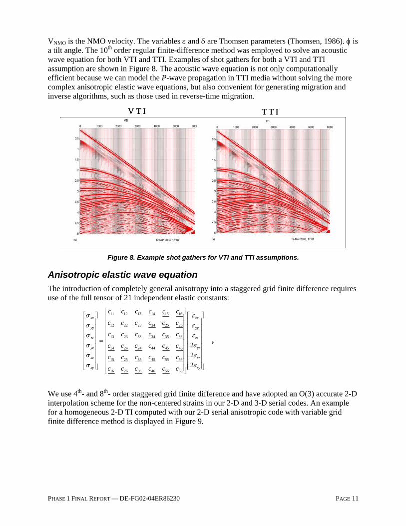
VNMO is the NMO velocity. The variables ε and δ are Thomsen parameters (Thomsen, 1986). φ is a tilt angle. The 10th order regular finite-difference method was employed to solve an acoustic wave equation for both VTI and TTI. Examples of shot gathers for both a VTI and TTI assumption are shown in Figure 8. The acoustic wave equation is not only computationally efficient because we can model the P-wave propagation in TTI media without solving the more complex anisotropic elastic wave equations, but also convenient for generating migration and inverse algorithms, such as those used in reverse-time migration.

Figure 8. Example shot gathers for VTI and TTI assumptions.

Anisotropic elastic wave equation The introduction of completely general anisotropy into a staggered grid finite difference requires use of the full tensor of 21 independent elastic constants:

11 12 13 14 15 16

12 22 23 24 25 26

13 23 33 34 35 36

14 24 24 44 45 46

15 25 35 45 55 56

16 26 36 46 56 66

222

xx xx

yy yy

zz zz

yz yz

xz xz

xy xy

c c c c c c

c c c c c c

c c c c c c

c c c c c c

c c c c c c

c c c c c c

σ εσ εσ εσ εσ εσ ε

⎡ ⎤⎡ ⎤ ⎡⎢ ⎥⎢ ⎥ ⎢⎢ ⎥⎢ ⎥ ⎢⎢ ⎥⎢ ⎥ ⎢⎢ ⎥=⎢ ⎥ ⎢⎢ ⎥⎢ ⎥ ⎢⎢ ⎥⎢ ⎥ ⎢⎢ ⎥⎢ ⎥ ⎢⎢ ⎥⎢ ⎥ ⎢⎣ ⎦ ⎣⎢ ⎥⎣ ⎦

⎤⎥⎥⎥⎥⎥⎥⎥⎥⎦

,

We use 4th- and 8th- order staggered grid finite difference and have adopted an O(3) accurate 2-D interpolation scheme for the non-centered strains in our 2-D and 3-D serial codes. An example for a homogeneous 2-D TI computed with our 2-D serial anisotropic code with variable grid finite difference method is displayed in Figure 9.

V T I T T IV T I T T I


Figure 9. Snapshot of particle velocity in shale.

Eikonal ray tracing FD solution of the eikonal equation is a very fast and accurate method to compute the traveltimes in complex velocity models. The FD eikonal solver can also provide easy visualization of wavefronts that can assist in interpreting seismic events in field data and synthetic data obtained from FDTD codes. We solved eikonal equations for isotropic, VTI and tilted TI media in the Celerity Domain. This code provides the first arrival traveltimes from the source.

The celerity is defined as:

),,()()()( 222

zyxtzzyyxx

tdC sss −+−+−== (2)

where ( sss zyx ,, ) are the coordinates and t is the traveltime from the source. By change of variables, the eikonal equation

),(2222

zxSzt

yt

xt

=⎟⎠⎞

⎜⎝⎛∂∂

+⎟⎠

⎞⎜⎝

⎛∂∂

+⎟⎠⎞

⎜⎝⎛∂∂

can be written in the form:

01))()()((2)( 222222

2

=−+−+−+−−++ SCCzzCyyCxxC

CCCCd

zsysxszyx

We use the finite difference and fast sweeping methods to solve the above equation. Figure 10 shows traveltime contours and relative error (in %) between the eikonal solver and analytic solution in a linear velocity gradient medium (vertical gradient of 0.1 s-1 with a velocity of 4000 m/s at the surface). The spacing is 125 m in both X- and Z-directions. Our numerical tests show that the new method is more accurate than the 2nd order fast marching method.


Figure 10. Top: Traveltime contours (in seconds). Bottom: relative error (in %) between eikonal solver and analytic solution in a linear velocity gradient medium (vertical gradient of 0.1 s-1 with a velocity of 4000 m/s at the surface). The spacing is 125 m in both X- and Z-directions.

Additions to the existing codes We also modified the codes listed above to incorporate:

A) Variable gridding for both vertical and horizontal directions We have applied this technique to isotropic acoustic and elastic wave equation, viscoelastic and anisotropic wave equation.

Recently, variable-grid finite difference methods have been developed to avoid spatial over-sampling when applied to multi-scale structures or large-scale structure with high velocity contrasts. For example, in the low velocity zones a fine grid is used and a coarse grid is employed for high velocity zones. In the variable grid method, the x grid spacing can vary in the x-direction and the z-spacing can vary in the z-direction, as shown in Figure 11.


Figure 11. Grid layout with nonuniform spacing.

In our new variable method, the spatial derivative is calculated by:

∑−=

∆+=∂

∂ N

Niij xxfa

xxf )()( ,

where ix∆ is the spatial increments. To determine the coefficients ja , we use a Taylor expansion of the above equation to obtain all coefficients.

We used a model with 460 x 460 grid points with the grid spacing changing from 1.375 to 2.75 m from left to right, and a time step of 2 ms. We used a P wave velocity of 2300 m/s, an S wave velocity of 1100 m/s and a density of 2100 kg/m3. Figure 12 shows the vertical velocity field sampled at 390 m from the source (a 20 Hz vertical body force). Excellent agreement is seen between the numerical and analytical results.

Figure 12. Comparison between numerical results and analytical solution for wave propagation in

a homogeneous model.


B) Attenuation incorporated (intrinsic constant Q) Attenuation can be incorporated into the staggered grid FDTD scheme via the memory variable approach (Day and Minster, 1984; Carcione et al., 1988; Robertsson et al., 1994; Komatitsch & Tromp, 1999). In the memory variable approach, general viscoelastic media are described as a superposition of K standard linear elastic solid elements each with their own relaxation times:

( )1

( ) 1 1 ( )m

iqrs

Kto m m

iqrs iqrsk

c t c e H tστε στ τ −

=

⎡ ⎤= − −⎢ ⎥

⎣ ⎦∑ . (3)

This general model allows the convolutional relationship between stress and strain,

( )( ) ( ) ( ) ( )

t iqrsiq iqrs rs rs

c tt c t t t dt

tσ ε ε

−∞

∂′ ′= ∗ = ∗

∂∫ , (4)

to be evaluated analytically. The resulting set of velocity-stress equations now includes the memory variable k

iqR that must be updated with the stresses,

( )

( )

1

1

( ) ( ) ( ) ( ) Viscoelastic Consitutive Relation

1( ) ( ) ( ) memory variable

1 modulus defect

unrelaxed modulus

Ku k

iq iqrs rs iqk

k kiq iqrs rs iqk

o k kiqrs iqrs iqrs

Ku oiqrs iqrs iqrs

k

t c t t R t

R t c t R t

c c

c c c

σ

ε σ

σ ε

δ ετ

δ τ τ

δ

=

=

= +

⎧= −

= −⎨

= −

∑

∑

&&&

&& &&

.

⎪⎪⎪

⎪⎪⎪⎩

(5)

The viscoelastic constitutive relation remains explicit in time and can model general anisotropic attenuation versus frequency behavior with minimum modifications to the stress update routines in the serial and parallel family of codes. The location and magnitude of the viscoelastic attenuation associated with each elastic constant is fully described by three parameters: the

stress relaxation time kστ , the strain relaxation times

kiqrsετ , and the relaxed (zero frequency)

moduli oiqrsc .

Anisotropic attenuation allows general loss to be associated with each elastic constant, as shown in Figure 13, at the additional computational expense of memory variable updates (3 in 2-D, 6 in 3-D) and the additional storage of a strain relaxation time for each elastic constant. A variable grid finite difference method is used to solve these wave equations.


(a) (b)

Figure 13. Snapshot of the P-wave in the VTI medium: (a) no attenuation, and (b) anisotropic attenuation in the vertical direction only (Qc33 = 20).

C) Perfectly matched layer (PML) absorbing boundary conditions The approach is variably staggered with any order finite difference method for anisotropic, elastic and variable-density acoustic wave equation. A variety of approaches haa been developed for absorbing waves on the model boundaries while generating minimum reflections. A simple and straightforward method consists of surrounding the model domain by a boundary zone N=20~30 grid points wide where the wavefield is gradually reduced to zero through the application of an exponential tapering function (Cerjan et al., 1985). A more sophisticated approach that requires N<16 grid points is the Perfectly Matched Layer (PML) approach of Berenger (1994). This approach has emerged as the method of choice for its effectiveness and minimal grid point requirements, and will be provided as an option in the seismic modeling engines developed for this project.

In the PML method, we split each variable into x and z or z, y and z directions. The PML formulations can be derived by a complex coordinate stretching approach expressed as:

xxidx ∂+⇒∂ ])(1[ω

, yyidy ∂+⇒∂ ])(1[ω

and zzidz ∂+⇒∂ ])(1[ω

where )(xd , )( yd and )(zd represent the exponential damping coefficients in the PML region along x , y and z , respectively. The equation of the horizontal particle velocity for 2-D wave equations

zxx

v xzxxx

∂∂

+∂∂

=∂∂ σσ

becomes

x

vxdxv xxx

x

xx

∂∂

=+∂∂ σ)(

z

vzdxv xzz

x

zx

∂∂

=+∂∂ σ)(

zx

xxx vvv +=


Usually, people take 2

2

23)1log()(

δδxV

Rxd P= , where PV is the velocity,δ is the thickness of the

PML and R is the theoretical reflection coefficient. As we can see from above equation, the PML method requires more memory than sponge methods. Figures 14(a) and (b) display the snapshot for a homogenous acoustic model with the PML and sponge absorbing boundary condition. There are no visible artificial reflections in the PML.

(a)

(b)

Figure 14. Comparison of PML (a) and sponge absorbing boundary conditions (b).

However, we found that using 2

2

23)1log()(

δδxV

Rxd P= is not a good choice in some cases because

it will introduce very low frequency components into our results. We will continue to work on this issue in Phase II.

D) Optimal coefficient finite difference We introduce a new method for designing optimized operators for staggered grid spatial differencing. Conventional staggered-grid FD coefficients are obtained from a Taylor’s series expansion that becomes progressively more inaccurate at higher wavenumbers. To obtain acceptable accuracy at these higher wavenumbers requires fine computational grids (typically 6-20 grids per wavelength). Tam and Webb (1993) showed for a standard (i.e., non-staggered grid)


FD scheme it is possible to obtain the optimized FD coefficients that result in fewer grid points per wavelength.

To obtain the optimized FD coefficients for a staggered grid FD scheme (Rector et al., 2002), a minimization of the numerical dispersion is performed over the modeled frequency band, as follows. The 2Nth order FD approximation for a staggered grid mesh is

1 ( (2 1) )2

N

jj N

f xa f x jx x =−

∂ ∆= + −

∂ ∆ ∑ , (7)

where x∆ is the grid spacing and N is the length of the differentiator. aj=a-j, j=1,2,...,N are the unknown FD coefficients. Taking the Fourier transform of Eq. (7) gives the effective wavenumber

(2 1) / 2N

i j k xj

j N

ik a ex

− ∆

=−

= −∆ ∑% , (8)

where k is the actual wavenumber. Minimizing the error over one wave cycle

),(2~

xkdxkxkE ∆∆−∆= ∫−π

π , (9)

and prescribing an acceptable error level (e.g., 0.01E ≤ ) yields FD coefficients with the minimal error over the frequency spectrum of the wavefield. Figure 15 shows the comparison between conventional 4th-order FD method and the new optimal FD method. Our new method has less dispersion. For O(4) spatial differencing, the number of grid points per wavelength for an error level of E=0.01 is 5.1 using the standard coefficients and 3.9 using the optimized coefficients. This difference translates into a memory savings of 30% in 2-D and 40% in 3-D, and approximately 34% less CPU time.

Figure 15. Comparison of the optimal and conventional FD.


Testing This section describes testing performed with the updated modeling codes and shows examples of using the modeling code produced during Phase I.

Timing tests We have tested some models to look at CPU times. Table 2 lists the CPU time for elastic and acoustic modeling with PML and elastic modeling with sponge absorbing condition.

TABLE 2

Examples Example 1: AVO It is well known that anisotropy can affect AVO responses, both in the estimation of incidence angles and in the modification of the reflection coefficients (Ruger, 1997). Using forward modeling that incorporates and omits anisotropy, we can examine the sensitivity of AVO to anisotropy. This allows us to investigate uncertainty in AVO inversions.

Figure 16 shows the velocity models: a finely layered and a smoothed, blocky model.


Figure 16. The velocity models: a finely layered and a smoothed, blocky model.

We generated a vertical transversely isotropic (VTI) model based on a finely layered velocity logs. To incorporate anisotropy, we assume 2.0=ε and 01.0=δ when the velocity is less than 3000 m/s and the depth is below 200 meters. Figure 17(a), (b) and (c) show a CMP gather generated for an elastic isotropic and an elastic anisotropic model and their difference, respectively. From Figure 17(c) we can see there are differences between anisotropic and isotropic results for both amplitude and traveltimes, particularly as the offset increases. The industry is pushing to larger and larger offsets to obtain accurate AVO inversions, and as offset increases, the effect of VTI properties also increases. Figure 18 shows the amplitude differences between isotropic and anisotropic model verse offset for the event at 0.93 s. This result implies that AVO inversion will result in erroneous parameters without including anisotropy.


17(a)

17(b)


17(c)

Figure 17. A CMP gather generated by finite difference method in isotropic (a) and anistropic model (b) and their difference (c).

Figure 18. The amplitude differences between isotopic and anisotropic model vs offset.

Example 2: Effect of Fine Layering on Attenuation Estimates Figure 19 shows seismograms in a fine layered and a smooth, blocky model and their differences, respectively. All receivers are located at the bottom of the model and a source is on the top of the model (if you wanted to do an offset VSP, you should really put the source at the


bottom and the receivers at the top). This example demonstrates that scattering attenuation due to thin layers has significantly affected amplitudes and traveltimes. For instance, the traveltime difference at zero-offset trace is about 3 ms and the amplitude and phase differences of the direct, downgoing arrival are substantial. The amplitude in the fine layering model is less than that in the smooth, blocky model. Also, AVO responses are different between these two models. The incorporation of fine layering such as this is not standard in many forward modeling routines, which may be part of the reason why forward models are not thought to be particularly realistic. We believe that our new tools will overcome many of these limitations.

19(a)

19(b)


19(c)

Figure 19. Seismograms generated by FD method in finely layered (a) and smoothed model (b) and their difference (c).

Example 3: Microseismic Monitoring Microseismic monitoring is rapidly becoming an accepted tool for monitoring reservoir production and such things as stimulation through hydraulic fracturing. Understanding the details of the earth wave propagation can be very important for locating and characterizing microseismic events. Studies performed on a hydrofrac in the late 1980’s (Ilderton, Rector, et al., 1994) show that lateral variation in the velocity field can dramatically modify the event locations.

Modeling microseismic events is complicated by fine layering and local heterogeneity. The last example we show models a microseismic event with and without fine layering. We assume that the source is at the depth 200 m and receivers are in a well. The offset is 600 m. Figure 20 shows the seismograms in a fine layering and a smoothed, blocky model. These result shows that fine layers have significant effect on traveltimes, for instance, at the depth 616 m the traveltime difference is about 7.8 ms.


(a) (b)

Figure 20. Seismograms with a finely layered model (a) and a smoothed, blocky model (b).

One important application for our finite difference modeling is to estimate the uncertainty for the inversions such as AVO. As inversion itself can not provide reasonable uncertainty estimation, we should run a set of models perturbed from inverted result to generate synthetic data. From these results we should obtain more accurate results for the uncertainty.

Conclusions and Recommendations In summary, the objectives of Phase I were fully met. No overriding feasibility issues remain in developing a commercial software package. The sections below describes some of the work that remains to introduce the commercial package originally envisioned in this project.

Technical Objectives for Future Work On future objective is to complete the seismic engine framework, to develop an initial prototype user interface for desktop application of the 2-D elements of the modeling codes, and to demonstrate the utility of the prototype package in solving real world problems. For a successful commercial development, an industry advisory group of recognized experts to help guide the development and to evaluate the prototype package by using it in real-world scenarios on their desktops is needed. . The specific tasks required in the future technical work include: • Develop the thin layer dynamic equivalent media approach • Complete the modeling engines highlighted in green in the table below • Incorporate arbitrary source and receiver positions by use of adaptive variable gridding • Incorporate user selected source mechanism and wavelets.


• Complete a market characterization study • Define prototype desktop 2-D modeling package specifications • Implement desktop prototype • Establish industry advisory panel • Conduct prototype evaluation with industry advisory panel • Conduct product focus group analysis to define commercial product(s) and services.

TABLE 3. FDTD SEISMIC MODELING: COMPLETED (√) & REMAINING (•)

SERIAL 2D

SERIAL 2.5D PML VARIABLE-

GRID SCATTERING ATTENUATION

Isotropic √ √ √ √ • TI √ √

ACOUSTIC

TTI √ √ Isotropic √ √ √ • TI √ Orthotropic

ELASTIC

Full Anisotropy √ √ √ • Isotropic √ √ • TI √ Orthotropic

VISCOELASTIC

Full Anisotropy • Isotropic √ TI √

EIKONAL

TTI √

Detailed Work Plan for Future Technical Work

Thin layer dynamic equivalent media It is well known that heterogeneity at a scale that is smaller than typical finite difference grid sizes (1/5 wavelength) has an effect on the traveltime and amplitude of seismic waves. Using finite difference method to model wave propagation in this thin layered model is very time consuming. One way of incorporating heterogeneity related to bedding is to utilize the well logs to create an effective medium by computing the auto and cross-correlations of material properties. These correlations can be incorporated into a dispersion relation based on the theoretical work of Shapiro and Zien (1993). One approach that will be investigated is to modify the finite difference stencil and create “physical” anisotropic dispersion as opposed to the numerical anisotropic dispersion. A second approach is to use the viscoelastic machinery


described above to match the anisotropic dispersion and attenuation that is associated with thin layering.

For the second approach, we derive a new acoustic wave equation that can model the scattering attenuation. The extrapolation operator for the downgoing wave is:

∑=

+ −−=m

kk

kmp cp

czjpzzW

1

220 )11exp(),;,( ωδω

and the attenuation term due to finely layer can be expressed as:

)cos)(exp( zAC neff ∆−= −αφω ,

where kc is the velocity of finely layer k and p is the ray parameter

)1()11(cos 222 pcp

c

ceffeff −=

><

><−=φ . α and n are constants.

We assume that we can use wave equation

2

2

2

22

2

22

tP

xPC

zPC HV ∂

∂=

∂∂

+∂∂ (10)

to model the scattering effects. We obtain:

ωω

jA

cCV

)(11+>=< (11)

]1)()(1[2

ω

ωα

jc

AnCcC VH

><

−+>=< (12)

We will derive a new wave equation based on Eq. (10), (11) and (12) in time domain and solve it with the variable-grid finite difference method. This new wave equation includes scattering attenuation effect but the coda cannot be seen in synthetic data. Compared to directly modeling the fine layered model, this method will be much faster.

Finalize modeling engines The goal over several years of development at LBL has been to complete a matrix of modeling engines providing full flexibility in both 2-D and 3-D modeling. In future technical work, the items shown in green in the table above will be completed.

Arbitrary source and receiver positions In the new world of reservoir seismic, sources and receivers will be deployed in exotic and irregular geometries dictated by wellbore geometries including highly deviated and horizontal well configurations. Initial versions of the seismic engines assumed regular source and receiver geometries. The variable gridding approach which is now an inherent part of the seismic engine framework will be enhanced with an adaptive variable grid to allow sources and receivers to occupy arbitrary positions.


Source types and wavelets The ability to generate arbitrary source mechanisms within the finite difference framework has been demonstrated as in the example generated in Phase 1 for a microseismic shear source. There are a number of source mechanism and source wavelets that could be implemented. Minimum and zero-phase Ricker, Llauder and Ormsby wavelets will be implemented. In addition, a maximally flat Butterworth wavelet (both minimum and zero phase) will be incorporated. These wavelets will be modifiable by differentiation, integration, constant phase rotation, and band-pass filtering.

Source mechanisms will include monopole (vertical or horizontal axis of activation), dipole, quadrapole, radial and vertical stress sources, pure pressure sources, and pure shear sources. Receiver mechanisms will be similar to source mechanisms. Source and receiver array effects will be created using interpolated grid node responses and appropriate weighted summation. A catalog of common source mechanisms will be generated and implemented to allow user control and selection of both source type and waveforms/wavelets including:

1. Source In seismic exploration, different sources are used in VSP, crosshole and surface reflection. A good forward modeling engines can model all these sources. In Phase II, we will incorporate monopole, dipole and quadrapole sources as well as plane wave sources in our engines.

For a monopole source, a single source point and source function are used. The source function is applied as a stress source at the given location, with equal x and z components. For a dipole source, two source points and two source functions are used. The second source function would have identical amplitudes but opposite polarity to the first source. The source functions are applied as x-directional velocity sources at the given locations. To generate a quadrapole source, we specify four source points and two different source functions. In this case we would use source functions with identical amplitudes and opposite polarity. Figure 21 shows the arrangement of the source points and the polarity of the source at each point.

Figure 21. Arrangement of the source points for a quadrapole source. Arrows show the polarity of the velocity source applied at each point.

We also will study how to model the borehole orbital vibrator source.

2. Fractures Modeling wave propagation in fractures is very important. Fractures are common within the subsurface and play a critical role in the mechanical and fluid flow properties of earth materials. In regions where the maximum compressive stress is vertical, open fractures will tend to be oriented vertically. The ability to interpret properties such as fracture spacing, orientation, and fluid content associated with such fracture systems is vital to the effective extraction and management of reservoir resources and the monitoring of contaminant migration. In particular,


the ability to delineate zones of high fracture density is a key component in developing reservoir-scale fluid flow models.

The way in which fractures affect seismic waves depends on mechanical parameters, such as compliance and saturating fluid, and on their geometric properties, such as dimensions and spacing. If fractures are small relative to the wavelength of the seismic waves, the waves will be only weakly affected by the fractures. If fractures have characteristic lengths on the order of the wavelength, then there will be scattering of energy due to the presence of the fractures. If fractures are spaced much closer than the wavelength of the seismic waves, then the medium will behave like a homogeneous, anisotropic equivalent medium. When fractures are spaced further away (about a quarter of a wavelength or more), the seismic waves will interact with the fractures and scatter appreciable energy from the wavefront.

The technique we adapt was proposed by Coates and Schoenberg (1995). The elastic properties of the discrete fractures are calculated using the Coates and Schoenberg (1995) thin anisotropic grid cell approach. The fractures are assumed to have negligible mass and thickness relative to the seismic wavelength in accordance with the linear slip model of Schoenberg (1980) for imperfect interfaces. We use the time domain, staggered variable grid finite difference to solve anisotropic stress-velocity formulation of the elastic wave equation.

Lateral heterogeneity In layered and heterogeneous media, the angular and frequency dependent seismic response is affected by the statistical distributions of physical properties. Investigations of the statistical nature of velocity and density perturbations may provide insights into mechanisms governing wave propagation as there may exist a strong correlation between the spatial properties of the velocity field of a reflective target and the lateral correlation length of the resulting seismic wave field. Reservoir zones are often characterized by strong perturbations in elastic parameters, in particular compressional wave velocities.

Forward modeling in heterogeneous media will help us to refine survey design and processing strategies of the VSP and borehole experiments, as well as to assess how well log data relate to the surrounding reservoir zone.

We construct stochastic random media using von Karman, exponential and Gaussian autocorrelation functions and their spectral density functions. If log data are available, some constants in autocorrelation functions, for instance, the correlation distance, can be determined by setting the power spectrum equal to that calculated by reflectivity from log data.


Technical references Aoi, S. & H. Fujiwara (1999). 3-D finite-difference method using discontinuous grids, Bull.

Seism. Soc. Am., 89(4), 918-930. Berenger, J.P. (1994). A perfectly matched layer for the absorption of electromagnetic waves, J.

Comp. Phys., 114, 185-200. Carcione, J.M., D. Kosloff & R. Kosloff (1988). Wave propagation simulation in a linear

viscoelastic medium, Geophys. J. R. Astro. Soc., 95, 597-611. Cerjan, C., D. Kosloff, R. Kosloff & M. Reshef (1985). A nonreflecting boundary condition for

discrete acoustic and elastic wave equations, Geophysics, 50, 705-708. Day, S.M. & J.B. Minster (1984). Numerical simulation of attenuated wavefields using a Pade

approximant method, Geophys. J. R. Astro. Soc., 78, 105-118. Driscoll, T.A. (2003). Radial basis functions for simulating PDE’s, online PDF presentation,

http://www.math.udel.edu/~driscoll/talks/rb/pde.pdf Graves, R.W. (1996). Simulating seismic wave propagation in 3-D elastic media using

staggered-grid finite differences, Bull. Seism. Soc. Am., 86, 1091-1106. Hestholm, S. (1999). Three-dimensional finite difference viscoelastic wave modeling including

surface topography, Geophy. J. Int., 139, 852-878. Igel, H., P. Mora & B. Riollet (1995). Anisotropic wave propagation through finite-difference

grids, Geophysics, 60(4), 1203-1216. Komatitsch, D. & J. Tromp (1999). Introduction to the spectral element method for three-

dimensional seismic wave propagation, Geophys. J. Int., 139, 806-822. Levander, A.R. (1988). Fourth-order finite difference P-SV seismograms, Geophysics, 53, 156-

168. Madariaga, R. (1976). Dynamics of an expanding circular fault, Bull. Seis. Soc. Am., 65, 163-

182. Mallick, S. & L.N. Frazer (1987). Practical aspects of reflectivity modeling, Geophysics, 52,

1355-1364. Pitarka, A. (1999). 3-D elastic finite-difference modeling of seismic ground motion using

staggered grids with nonuniform spacing, Bull. Seism. Soc. Am., 89, 575-596. Rector, J., Zhang, L. and Hoversten, G., 2002, Optimized Coefficient Finite Difference Scheme

For Wave Equation, SEG workshop, 72st Ann. Internat. Mtg., Soc. Expl. Geophys. Robertsson, J.O.A., J.O. Blanch & W.W. Symes (1994). Viscoelastic finite difference modeling,

Geophysics, 59(9), 1444-1456. Saenger, E.H., N. Gold & S.A. Shapiro (2000). Modeling the propagation of elastic waves using

a modified finite-difference grid, Wave Motion, 31, 77-92. Shapiro, S.A.. & H. Zien (1993). The O’Doherty-Anstey formula and localization of seismic

waves, Geophysics, 58, 736-740. Song, Z.-M. & P.R. Williamson (1995). Frequency-domain acoustic wave modeling and

inversion of crosshole data: Part I—2.5-D modeling method, Geophysics, 60(3), 784-795.


Tam, C.K.W. & J.C. Webb (1993). Dispersion-relation-preserving finite difference schemes for computational acoustics, J. Comp. Phys., 107, 262-281.

Vireaux, J. (1986). P-SV wave propagation in heterogeneous media: Velocity-stress finite difference method, Geophysics, 51, 889-901.

Yee, K.S. (1966). Numerical solution of initial boundary values problems involving Maxwell’s equations in isotropic media, IEEE Trans. Antennas and Propagation, 14, 302-307.

Zhang, L., Rector, J. and Hoversten, G., 2002, An eikonal solver in tilted TI media: 72st Ann. Internat. Mtg., Soc. Expl. Geophys., (1955-1958)

seismic modeling engines phase 1from north america will come from land reservoirs. if geophysics is...

Documents