seismic field data processing example - ahay.org · 1 seismic field data processing...

1

Seismic field data processing example-- Tutorial of Madagascar --

Yang LiuCollege of Geo-exploration Science and Technology,

Jilin University08/15/2013

[email protected]

http://www.ahay.org

2

Outline

Dive into Madagascar

Assignment

Field data example

3

Outline


Assignment

Field data example

4


• Using Self-document– Find which module you want to use

by “sfdoc –k keyword”

– Read self-document by just running module name and find parameters, examples, and source code.

– Command-line Test

sfspike n1=1000 k1=300 | sfbandpass fhi=2 phase=1 | \

sfwiggle clip=0.02 title="Welcome to Madagascar" | sfpen

• Following examples is the best way to learn.– Everything is reproducible.

5

Outline


Assignment

Field data example

6

Assignment

Crucial Problems for different types of data:Land data: Statics correction, SNR, etc.

Marine data: Interpolation, Multiples, migration, etc.

The tutorial is given to set up a processing workflow for a field land data.

Field seismic data are always complicated!

7

Outline


Assignment

Field data example

8

Tutorial workflow

Get data and convert to RSF formatInitial data checkingInitial signal analysis and quality control

Statics correctionFirst break muteSubsampling with anti-aliasing filterGround-roll attenuation

Convert from CSP to CMPVelocity analysisNMO and brute stackingToy migration

9

The first step to do:

• Open a new text file and name it as “SConstruct”.

• Begin to write your script for workflow.

10

Get data and convert to RSF format

from rsf.proj import *

tgz = '2D_Land_data_2ms.tgz'

Fetch(tgz,server='http://www.freeusp.org',top='RaceCarWebsite/TechTransfer/Tutorials/Processing_2D',dir='Data')

files = map(lambda x: 'Line_001. '+x,Split('TXT SPS RPS XPS sgy'))

Flow(files,tgz,'gunzip -c $SOURCE | tar -xvf -',stdin=0,stdout=-1)

Flow('line tline','Line_001.sgy','segyread tfile=${TARGETS[1]}')

Always start here!Always start here!

If you have had the data in the If you have had the data in the directory, comment these lines.directory, comment these lines.

11

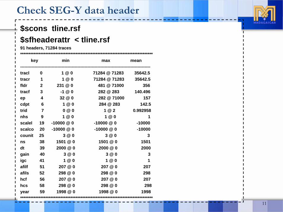
$scons tline.rsf$sfheaderattr < tline.rsf91 headers, 71284 traces*******************************************************************************

key min max mean-------------------------------------------------------------------------------------------tracl 0 1 @ 0 71284 @ 71283 35642.5tracr 1 1 @ 0 71284 @ 71283 35642.5fldr 2 231 @ 0 481 @ 71000 356tracf 3 -1 @ 0 282 @ 283 140.496ep 4 32 @ 0 282 @ 71000 157cdpt 6 1 @ 0 284 @ 283 142.5trid 7 0 @ 0 1 @ 2 0.992958nhs 9 1 @ 0 1 @ 0 1scalel 19 -10000 @ 0 -10000 @ 0 -10000scalco 20 -10000 @ 0 -10000 @ 0 -10000counit 25 3 @ 0 3 @ 0 3ns 38 1501 @ 0 1501 @ 0 1501dt 39 2000 @ 0 2000 @ 0 2000gain 40 3 @ 0 3 @ 0 3igc 41 1 @ 0 1 @ 0 1afilf 51 207 @ 0 207 @ 0 207afils 52 298 @ 0 298 @ 0 298hcf 56 207 @ 0 207 @ 0 207hcs 58 298 @ 0 298 @ 0 298year 59 1998 @ 0 1998 @ 0 1998*******************************************************************************

Check SEG-Y data header

12

Initial data checking

Result('first','line','''window n2=1000 | agc rect1=250 rect2=100 |grey title="First 1000 traces“font=2 labelsz=6 labelfat=4''')

$sfin line.rsfline.rsf:

in="/your directory/line.rsf@"esize=4 type=float form=native n1=1501 d1=0.002 o1=0 label1="Time" unit1="s" n2=71284 d2=1 o2=0 label2="Trace“

106997284 elements 427989136 bytes

13

lines = {'S':251,'R':782}color = {'S':4, 'R':2}for case in 'SR':

# X-Y geometryFlow(case+'.asc','Line_001.%cPS' % case,

'''awk 'NR > 20 {print $8, " ", $9}' ''')Flow(case,case+'.asc',

'''echo in=$SOURCE data_format=ascii_float n1=2 n2=%d | dd form=native ''' % lines[case],stdin=0)

Plot(case,'''scale dscale=0.001 | dd type=complex |graph symbol=* title=%c plotcol=%dmin1=684 max1=705 min2=3837 max2=3842''' % (case,color[case]))

True geometry

14

Plot('s118', 'S','''window n2=1 f2=118 | scale dscale=0.001 | dd type=complex |graph symbol=O wanttitle=n plotcol=3 symbolsz=4 plotfat=10min1=684 max1=705 min2=3837 max2=3842''')

Result('SRO','R S s118','Overlay')

Plot shots and receivers position

15

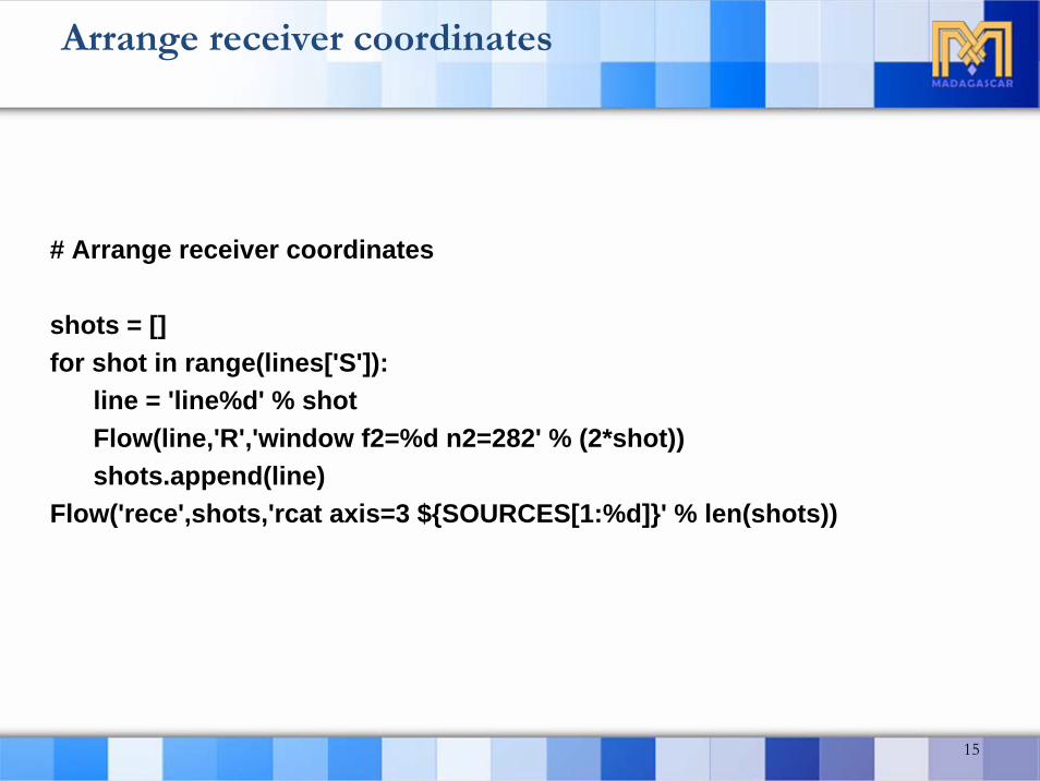
# Arrange receiver coordinates

shots = []for shot in range(lines['S']):

line = 'line%d' % shotFlow(line,'R','window f2=%d n2=282' % (2*shot))shots.append(line)

Flow('rece',shots,'rcat axis=3 ${SOURCES[1:%d]}' % len(shots))

Arrange receiver coordinates

16

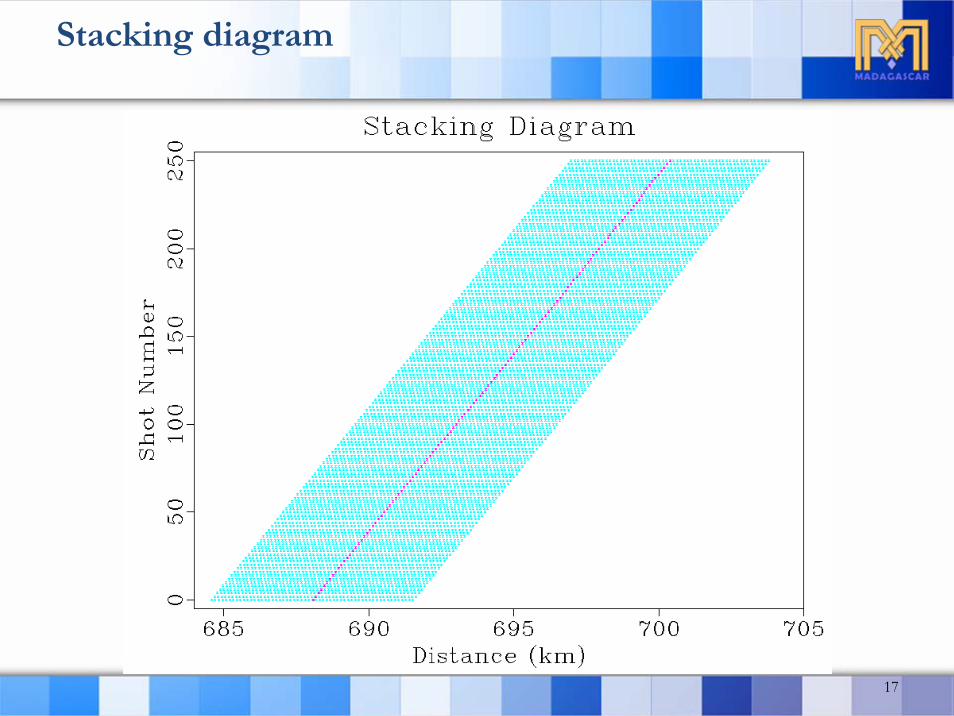
Plot('rec', 'rece','''window n1=1 j2=5 j3=2 | scale dscale=0.001 |rtoc | math output="input+I*x2" |graph symbol=* plotcol=%d title="Stacking Diagram"label1=Distance unit1=km label2="Shot Number"min1=684 max1=705''' % color['R'])

Plot('sou', 'S','''window n1=1 j2=2 | scale dscale=0.001 |rtoc | math output="input+I*x1" |graph symbol=* plotcol=%d wanttitle=n wantaxis=n min1=684 max1=705''' % color['S'])

Result('diagram', 'rec sou', 'Overlay')

Plot stacking diagram

17

Stacking diagram

18

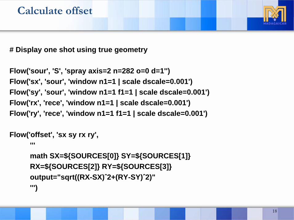
# Display one shot using true geometry

Flow('sour', 'S', 'spray axis=2 n=282 o=0 d=1'')Flow('sx', 'sour', 'window n1=1 | scale dscale=0.001')Flow('sy', 'sour', 'window n1=1 f1=1 | scale dscale=0.001')Flow('rx', 'rece', 'window n1=1 | scale dscale=0.001')Flow('ry', 'rece', 'window n1=1 f1=1 | scale dscale=0.001')

Flow('offset', 'sx sy rx ry','''math SX=${SOURCES[0]} SY=${SOURCES[1]}RX=${SOURCES[2]} RY=${SOURCES[3]}output="sqrt((RX-SX)ˆ2+(RY-SY)ˆ2)"''')

Calculate offset

19

Flow('lines', 'line','''intbin xk=cdpt yk=fldr | window f2=2 |putlabel3=Source d3=0.05 o3=688 unit3=kmlabel2=Offset d2=0.025 o2=-3.5 unit2=kmlabel1=Time unit1=s''')

Result('lines','''transp memsize=1000 plane=23 | byte gainpanel=each |grey3 frame1=500 frame2=100 frame3=120 flat=ntitle="Raw Data"''')

[yourcomputer directory]$ sfin lines.rsflines.rsf:

in="$RSFDATA/.../.../lines.rsf@"esize=4 type=float form=nativen1=1501 d1=0.002 o1=0 label1="Time" unit1="s" n2=282 d2=0.025 o2=-3.5 label2="Offset" unit2="km" n3=251 d3=0.05 o3=688 label3="Source" unit3="km"

106243782 elements 424975128 bytes

Map to regular shot gathers

2-D shot gathers (assuming regular coordinates)

20

21

Flow('shot118', 'lines', 'window n2=1 f2=118')Flow('offset118', 'offset', 'window n2=1 f2=118')Flow('boff1', 'offset118', 'window n1=141 | math output="-input"')Flow('boff2', 'offset118', 'window f1=141')Flow('boff118','boff1 boff2', 'cat axis=1 ${SOURCES[1]} ')Result('shot118', 'shot118 boff118',

'''agc rect1=50 rect2=50 |wiggle xpos=${SOURCES[1]} transp=y yreverse=y poly=ywherexlabel=t wheretitle=b title="Shot 118"''')

Plot No. 118 shot gather using true geometry

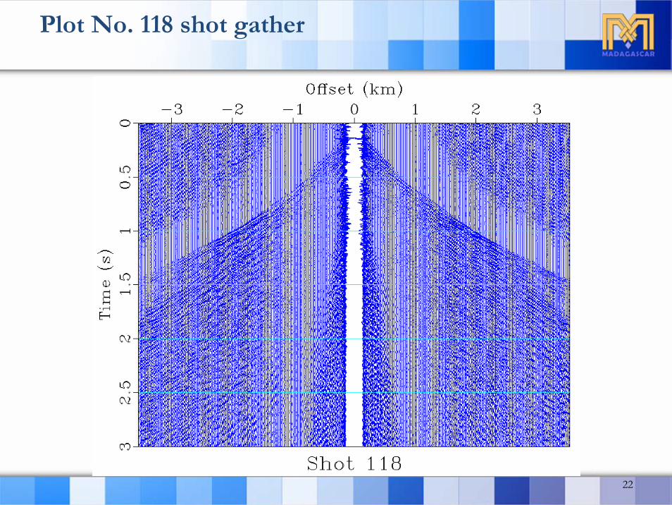
Plot No. 118 shot gather

22

23

Flow('rcmps mask', 'lines','''shot2cmp mask=${TARGETS[1]} half=n |put o2=-1.75 d2=0.05 label2="Half-offset"''')

Result('rcmps','''byte gainpanel=each | window j3=3 |grey3 frame1=500 frame2=35 frame3=214 flat=npoint1=0.8 point2=0.4 title="CMPs" ''')

Convert shots to CMPs(assuming regular geometry, improve by yourself)

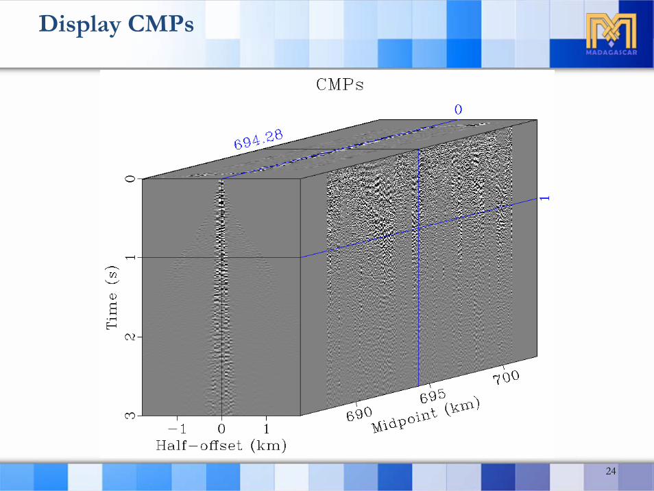
Display CMPs

24

25

Flow('fold', 'mask', 'dd type=float | stack axis=1 norm=n')Flow('rstack', 'rcmps', 'stack')Result('rstack', 'fold rstack',

'''spray axis=1 n=1501 d=0.002 o=0 label=Time unit=s |add scale=1,1000 ${SOURCES[1]} |grey color=j title="Raw Stack (with Fold)"''')

Raw stacking

Raw stacking

26

27

for case in 'SR':stat = case+'-statics'Flow(stat+'.asc','Line_001.%cPS' % case,'''awk 'NR > 20 {print $10}' ''')Flow(stat,stat+'.asc',

'''echo in=$SOURCE data_format=ascii_float n1=%d | dd form=native |scale dscale=%g | put label=Time unit=s''' % (lines[case],1./1900),stdin=0)

Applying statics corrections

28

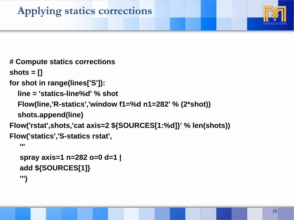
# Compute statics correctionsshots = []for shot in range(lines['S']):

line = 'statics-line%d' % shotFlow(line,'R-statics','window f1=%d n1=282' % (2*shot))shots.append(line)

Flow('rstat',shots,'cat axis=2 ${SOURCES[1:%d]}' % len(shots))Flow('statics','S-statics rstat',

'''spray axis=1 n=282 o=0 d=1 |add ${SOURCES[1]}''')


29

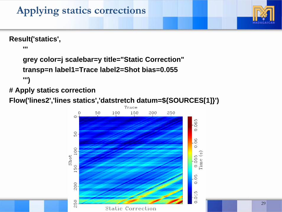
Result('statics','''grey color=j scalebar=y title="Static Correction"transp=n label1=Trace label2=Shot bias=0.055''')

# Apply statics correctionFlow('lines2','lines statics','datstretch datum=${SOURCES[1]}')


30

# Select 4 shots every tenth sequential shot

Flow('inpmute', 'lines2','''window f2=198 j2=10 n3=4''')

Result('inpmute','''put n2=1128 n3=1 |agc rect1=50 rect2=20 | grey wanttitle=n''')

First break mute

Input

31

32

# Select muting parameter for background noise

Flow('outmute', 'inpmute','''mutter t0=0. v0=5.2''')

Result('outmute','''put n2=1128 n3=1 |agc rect1=50 rect2=20 | grey wanttitle=n''')

First break mute

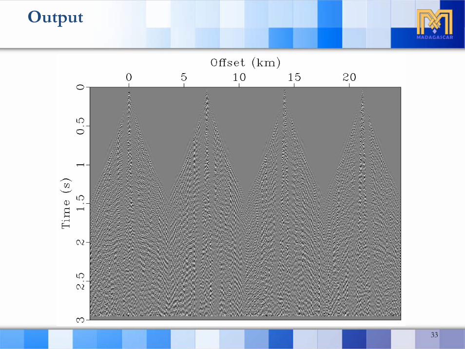
Output

33

34

# First break muting for all shots

Flow('mutes', 'lines2','''mutter t0=0. v0=5.2 |''')

Apply muting on all shots

35

# Shot 198Flow('shot198', 'mutes', 'window n3=1 f3=198')Plot('shot198', 'grey title="Shot 198" labelfat=4 titlefat=4')

# SpectraFlow('spec198', 'shot198', 'spectra2’)Plot('spec198',

'''grey color=j yreverse=n title="Spectra 198" bias=0.08label1=Frequency unit1=Hz label2=Wavenumber unit2=1/kmlabelfat=4 titlefat=4''')

Result('input198', 'shot198 spec198', 'SideBySideAniso')

Subsampling – input

36

Input

37

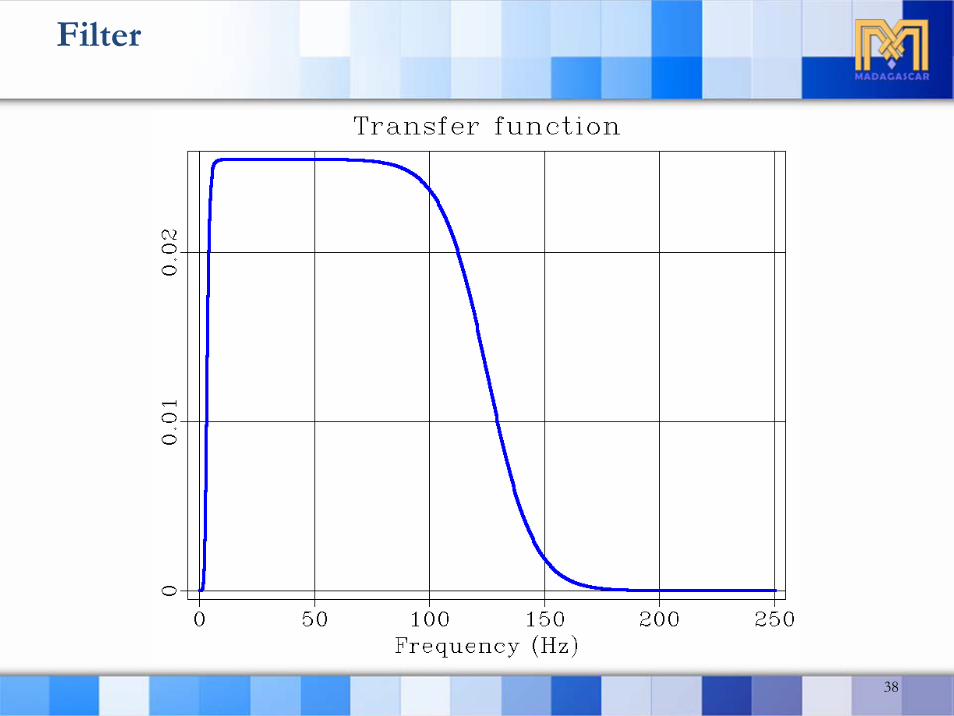
# Test anti-aliasing filterFlow('spike',None, 'spike n1=1501 d1=0.002 o1=0 k1=750 mag=1 nsp=1')Flow('bandp', 'spike', 'bandpass flo=3 fhi=125 nphi=8')Result('sbandp', 'bandp',

'''spectra |graph title="Transfer function"labelsz=8 plotfat=10 grid=y''')

Subsampling – antialiasing filter design

38

Filter

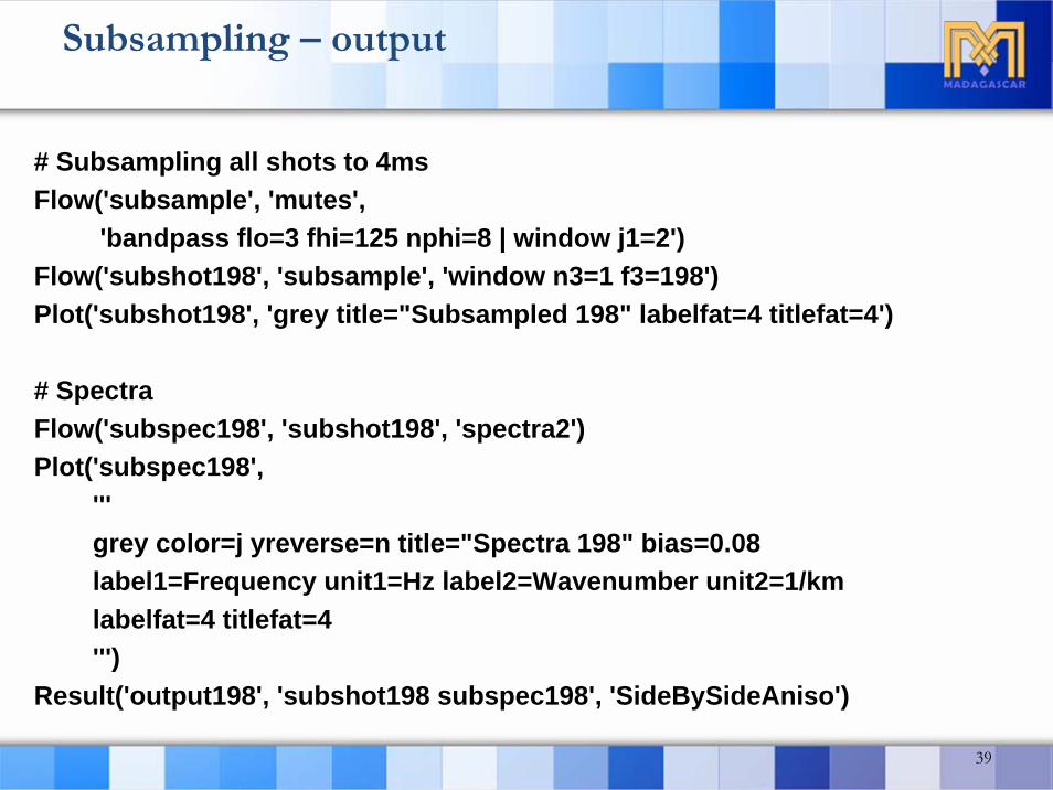
39

# Subsampling all shots to 4msFlow('subsample', 'mutes',

'bandpass flo=3 fhi=125 nphi=8 | window j1=2')Flow('subshot198', 'subsample', 'window n3=1 f3=198')Plot('subshot198', 'grey title="Subsampled 198" labelfat=4 titlefat=4')

# SpectraFlow('subspec198', 'subshot198', 'spectra2')Plot('subspec198',

'''grey color=j yreverse=n title="Spectra 198" bias=0.08label1=Frequency unit1=Hz label2=Wavenumber unit2=1/kmlabelfat=4 titlefat=4''')

Result('output198', 'subshot198 subspec198', 'SideBySideAniso')

Subsampling – output

40

Output

41

Flow('ltft198', 'subshot198','''ltft rect=20 verb=n nw=50 dw=2 niter=50''')

Result('ltft198','''math output="abs(input)" | real |byte allpos=y gainpanel=100 pclip=99 |grey3 color=j frame1=120 frame2=7 frame3=71 label1=Time flat=yunit1=s label3=Offset label2="\F5 f \F-1" unit3=kmscreenht=10 screenratio=0.7 parallel2=n format2=%3.1fpoint1=0.8 point2=0.3 wanttitle=n labelfat=4 font=2 titlefat=4''')

Calculate time-frequency spectra

42

Time-frequency (TF) spectra

Thresholding

Flow('thr198', 'ltft198','''transp plane=23 memsize=1000 |threshold2 pclip=25 verb=y |transp plane=23 memsize=1000''')

Result('thr198','''math output="abs(input)" | real |byte allpos=y gainpanel=100 pclip=99 |grey3 color=j frame1=120 frame2=7 frame3=71 label1=Time flat=yunit1=s label3=Offset label2="\F5 f \F-1" unit3=kmscreenht=10 screenratio=0.7 parallel2=n format2=%3.1fpoint1=0.8 point2=0.3 wanttitle=n labelfat=4 font=2 titlefat=4''')

43

44

Thresholded TF spectra

Signal and noise separation

Flow('noise198', 'thr198', 'ltft inv=y | mutter t0=-0.5 v0=0.7')Plot('noise198',

'grey title="Ground-roll 198" unit2=km labelfat=4 titlefat=4')

Flow('signal198', 'subshot198 noise198', 'add scale=1,-1 ${SOURCES[1]} ')Plot('signal198',

'grey title="Ground-roll removal" labelfat=4 titlefat=4')Result('sn198', 'signal198 noise198', 'SideBySideAniso')

45

Signal and noise separation

46

Process the whole dataset (cheating here!)

Flow('noise','subsample','''threshold2 pclip=20 verb=y''')

Flow('signals','subsample noise','add scale=1,-1 ${SOURCES[1]}‘)

47

Process the whole dataset (try by yourself)

## # Apply LTFT on entire 2-D line## Flow('ltfts', 'subsample',## '''## ltft rect=20 verb=y nw=50 dw=2 niter=50## ''',split=[3,282],reduce="cat axis=4")## Flow('thresholds', 'ltfts',## '''## transp plane=23 memsize=1000 | threshold2 pclip=25 verb=y |# # transp plane=23 memsize=1000## ''',split=[3,251])## Flow('noise', 'thresholds',## '''## ltft inv=y |## mutter t0=-0.5 v0=0.7 |## ''')## Flow('signals', 'subsample noise', 'add scale=1,-1 ${SOURCES[1]} ')

48

Convert shots to CMPs(assuming regular geomety, improve by yourself)

# Convert shots to CMPsFlow('cmps', 'signals',

'''mutter v0=3. |shot2cmp half=n | put o2=-1.75 d2=0.05 label2="Half-offset"''')

Result('cmps','''byte gainpanel=each |grey3 frame1=500 frame2=36 frame3=642 flat=ntitle="CMP gathers" point1=0.7 label2=Offset label3=Midpoint''')

49

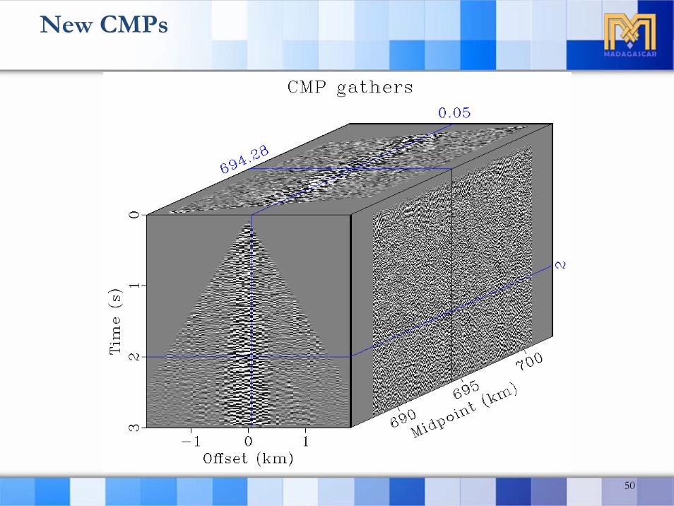
New CMPs

50

Velocity scan

# Set up velocity scan parametersv0 = 1.0dv = 0.05nv = 75

51

Velocity scan for all CMPs

# Velocity scanning for all CMP gathersFlow('scn', 'cmps',

'''vscan semblance=y v0=%g nv=%d dv=%g half=y str=0 |mutter v0=0.9 t0=-4.5 inner=y''' % (v0,nv,dv),split=[3,1285])

Flow('vel', 'scn', 'pick rect1=15 rect2=25 gate=100 an=10 | window')Result('vel',

'''grey title="NMO Velocity" label1="Time" label2="Lateral"color=j scalebar=y allpos=y bias=2.1 barlabel="Velocity"barreverse=y o2num=1 d2num=1 n2tic=3 labelfat=4 font=2 titlefat=4''')

52

Display NMO velocity

53

Normal moveout (NMO)

# NMOFlow('nmo', 'cmps vel',

'''nmo velocity=${SOURCES[1]} half=y''')

Result('nmo','''byte gainpanel=each |grey3 frame1=500 frame2=36 frame3=642 flat=ntitle="NMOed Data" point1=0.7label2=Offset label3=Midpoint''')

54

Display NMOed CMPs

55

Brute stack

# Brute stacking

Flow('bstack', 'nmo', 'stack')Result('bstack',

'''agc rect1=50 |grey title="Brute stacking" labelfat=4 font=2 titlefat=4''')

56

Display brute stacking result

57

Toy prestack Kirchhoff time migration

# Prestack Kirchhoff time migrationFlow('tcmps', 'cmps', 'transp memsize=1000 plane=23')Flow('pstm', 'tcmps vel',

'''mig2 vel=${SOURCES[1]} apt=5 antialias=1''',split=[3,71,[0]],reduce=’add’)

Result('pstm','''grey title="Prestack kirchhoff time migration"labelfat=4 font=2 titlefat=4''')

End()

58

Always stop here!Always stop here!

Display migration result

59

To be continued ...

Modify/add your own modules, improve the final result …

Try “scons view” to see all figures one by one.

60

61

Software

http://www.ahay.org

seismic field data processing example - ahay.org · 1 seismic field data processing...

Documents