seismic characterization of water masses and mesoscale ... · 44 seismic oceanography, subtropical...

Seismic characterization of water masses and mesoscale eddies associated with 1

the subtropical front SE of New Zealand 2

3

4

Andrew R. Gorman, Matthew W. Smillie, Joanna K. Cooper, M. Hamish Bowman, Department of 5

Geology, University of Otago, Dunedin, New Zealand 6

7

Ross Vennell, Department of Marine Science, University of Otago, Dunedin, New Zealand 8

9

Steve Holbrook, Department of Geology and Geophysics, University of Wyoming, Laramie, USA 10

11

Russell Frew, Department of Chemistry, University of Otago, Dunedin, New Zealand 12

13

Corresponding author: Andrew R. Gorman, Department of Geology, University of Otago, PO Box 14

56, Dunedin 9054, New Zealand. ([email protected]) 15

16

Draft Date: 17 April 2014 17

18

19

Key Points 20

• Seismic oceanography images water masses adjacent to the Subtropical Front 21

• Eddies are shown to be mixing water in vicinity of Subtropical Front 22

• Submarine water mass boundaries are more stable than surface expressions 23

Seismic Oceanography of the Subtropical Front SE of New Zealand 2

Abstract 24

The Subtropical Front, a major global boundary separating subtropical and subantarctic waters, is 25

locally diverted to the south by the New Zealand landmass. In this region, large volumes of 26

dissolved or suspended material are intermittently transported across the front; however, the 27

mechanisms of such transport processes are enigmatic. Existing maps and cross-sections of such 28

oceanic boundaries generally depend on measurements collected from stationary points on the 29

ocean surface or seafloor. The details of these datasets, which are critical for understanding how 30

water masses interact and mix at the fine- (< 10 m) to mesoscale (10 to 100 km), are poorly 31

constrained due to resolution considerations. The new method of seismic oceanography, applied to 32

serendipitously located multi-channel seismic data, provides detailed images of reflectivity 33

associated with oceanic water masses. Three nearly coincident profiles have been reprocessed to 34

produce remarkable images of three main water masses, the boundaries between them, and 35

associated thermohaline fine-structure. Interpretations of the data show that the Subtropical Front is 36

a zone that dips landward, with a width that can vary between summer and autumn by as much as 37

20 km. The boundary zone between subantarctic waters and the underlying antarctic intermediate 38

waters is also observed to dip landward. Several isolated lenses have been identified on the three 39

data sets, ranging in size from 9 to 30 km in diameter. These lenses are interpreted as mesoscale 40

eddies that form at depth in the vicinity of the Subtropical Front. 41

42

Index Terms 43

Seismic oceanography, Subtropical Front, mesoscale eddy, Southland Current, subantarctic water 44

45


1. Introduction 46

The Subtropical Front (STF) off the SE coast of New Zealand [Heath, 1981; 1985; Rickard et al., 47

2005] is an enigmatic ocean boundary that separates subtropical waters (STW) that are generally 48

warm, low in nutrients, and sustain high levels of phytoplankton growth (primary productivity) 49

from subantarctic waters (SAW) that are generally cold, high in nutrients, and low in productivity 50

(Figure 1). As roughly a third of New Zealand’s offshore waters are associated with the circumpolar 51

subantarctic water mass [Murphy et al., 2001] (comprising about 10% of the world’s oceans), this 52

region is ideally positioned for studying the interaction of this water body with subtropical waters to 53

the north. 54

55

The region of the ocean south of the Chatham Rise regularly exhibits unexpectedly sustained 56

productivity across the STF. This region can be considered a natural laboratory for studying a 57

global phenomena involving the oceanic transport of iron that episodically plays a determining role 58

in increased productivity [Boyd et al., 1999; Boyd et al., 2000; Boyd, 2004; Boyd et al., 2004]. 59

These enhanced productivity events can be stimulated by sporadic iron supply mechanisms [Banse 60

and English, 1997], such as dust storms [DiTullio and Laws, 1991; Husar et al., 2001] and eddy-61

driven transport of iron-rich coastal waters to offshore regions [Whitney and Robert, 2002]. 62

However, iron carried in airborne dust has been ruled out as the mechanism for this productivity 63

[Boyd et al., 2004], which implies that significant ocean mixing must be occurring here to transfer 64

iron across the front. 65

66

To understand the processes involved with mixing ocean water masses, we need to finely sample 67

and model properties such as bathymetry, fluid composition, temperature, and current velocity 68

[Davis, 1991; de Ronde et al., 2005; Robinson and Eakins, 2006; Smith and Sandwell, 1994; 69


Vanneste et al., 2006; Vennell, 1994; 1998]. High-resolution observations of these water properties 70

have improved greatly in the last 20 years. However, these measurements generally are made by 71

tools that are either (a) dropped from stationary boats or (b) attached to floating or seabed moorings. 72

These measurements require synthesis and interpolation to produce laterally-continuous 73

representations. Measurements of chemical parameters are even sparser because they usually rely 74

on the shipboard collection of samples that are processed after a cruise. In our target area, these 75

observations are incapable of answering basic questions such as, ‘How much water is involved in a 76

mixing event?’ or ‘Does the water mix as the result of an eddy or an upwelling tongue?’ 77

78

The emergence of the field of seismic oceanography [Holbrook et al., 2003; Holbrook et al., 2006; 79

Nandi et al., 2004; Páramo and Holbrook, 2005; Tsuji et al., 2005; Wood et al., 2008] has enabled 80

the visualization of oceanic water masses in the same way and with the same data that sedimentary 81

basins are imaged in the sea floor. Investigations of the geology of continental margins by the 82

petroleum industry over the last few decades contain a wealth of unexploited information on ocean 83

water masses above the seafloor. Fine-scale variations in temperature and, perhaps, salinity 84

manifest themselves as sound-seed contrasts; conventional seismic reflection methods record such 85

variability with a vertical resolution of ~10 m and a sensitivity to abrupt temperature contrasts as 86

small as 0.05°C [Holbrook et al., 2006]. Simple processing techniques readily produce clear images 87

of ocean structures that were below the visible threshold in previous versions of the seismic data 88

processed to show sub-seafloor geology. A range of oceanographic features has been investigated 89

including the evolution and dispersal of large eddies (e.g., Meddies at the mouth of the 90

Mediterranean [Biescas et al., 2008]), the position and variability of ocean boundary currents (e.g., 91

the Agulhas Current off the Cape of Good Hope [Uenzelmann-Neben et al., 2008]), and dynamics 92

of internal waves occurring on boundaries between ocean layers with different densities, 93


temperatures and salinities (e.g., interaction of internal waves with continental shelf sediments at 94

the Rockall Trough off Ireland [Jones et al., 2010]). Existing oceanographic methods are incapable 95

of observing the the fine detail of such processes due to their sporadic and spatially–constrained 96

nature. 97

98

In this paper, we present detailed cross-sectional seismic images of the water masses spanning a 99

section of the Subtropical Front – as they mix – using multi-channel seismic data collected by the 100

petroleum industry for deeper geological targets. We capitalise on recent petroleum exploration 101

efforts SE of New Zealand to analyze data showing the temporal and spatial characteristics of water 102

masses on either side of the Subtropical Front and indications of dynamic mixing processes 103

underway as the result of mesoscale eddies. 104

105

2. Seismic data acquisition and processing 106

Recent hydrocarbon exploration efforts SE of New Zealand have led to the acquisition of several 107

extensive seismic surveys in the region of the Subtropical Front (Fig.1). The DUN-06 2D seismic 108

survey was undertaken by the New Zealand government to encourage petroleum exploration in the 109

Great South Basin prior to an exploration block offer made in 2007. This then led to the acquisition 110

of the OMV-08 2D seismic survey (and additional on-going exploration efforts). Both surveys 111

contain seismic lines suitable for imaging oceanographic features across the Subtropical Front. A 112

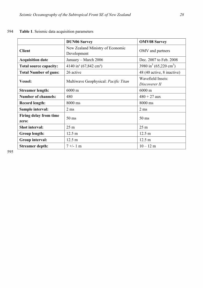
summary of the acquisition parameters of the DUN-06 and OMV-08 surveys is provided in Table 1. 113

114

Three parallel seismic lines from the two surveys (lines DUN-06-13, OMV-08-45, and OMV-08-115

42) are presented here to highlight the oceanographic features visible in these data and to 116

investigate the spatial and temporal variability of such features. The lines were chosen from these 117


datasets with optimal orientations for examining the water mass extending from the shallow shelf to 118

moderately deep waters of the Campbell Plateau at the south end of New Zealand’s South Island 119

(Fig. 1). DUN-06-13 lies parallel to and halfway between OMV-08-42 and OMV- 08-45. The main 120

difference in the survey designs is the airgun arrays used during the acquisition (a 26-gun array for 121

DUN-06 compared to a 48-gun array for OMV-08), but the energy of the airguns was similar (just 122

over 65 L for both surveys). 123

124

Processing of these data has focused on the water column, rather than the sub-seafloor geology for 125

which the data were originally collected [Smillie, 2012]. These datasets span the continental shelf, 126

slope and rise in water depths from a few metres to more than 1500 m; they are optimally located 127

for investigations of water variability caused by interactions between shoreline processes and deep-128

water currents. Processing of the seismic data followed a fairly routine flow that focuses on water 129

column reflectivity [cf. Nandi et al., 2004; Pinheiro et al., 2010] using petroleum industry software 130

[Ravens, 2001], including pre-stack deconvolution, manual trace editing, removal of the direct 131

arrival, detailed velocity analysis, seafloor muting, and NMO correction; post-stack flow included a 132

simple band-pass filter and finite difference migration. Amplitude gain was addressed by applying a 133

spherical divergence operator based on the final velocity model. The processed sections are shown 134

in Fig. 2. 135

136

3. Detailed seismic observations 137

3.1 Reflection variability 138

In seismic oceanography reflection sections, laterally coherent reflections occur as a result of 139

relatively abrupt changes in acoustic impendence (the product of sound speed and water density). 140

These changes predominantly arise from thermohaline contrasts, which advect laterally along 141


isopycnals. Isopycnals can be assumed to have very shallow spatial gradients [Cox, 1987] and 142

therefore, reflections are typically observed to be sub-horizontal. Coherent reflections can extend 143

horizontally for >10 km as can be seen in the reflective zones associated with regions of increased 144

temperature variability. Such reflections (e.g., the Southland Current (SC) and transition zone (TZ) 145

regions of Fig. 2) likely correspond to waters lying between more stable water masses. Reflections 146

also can be short (<100 m), like the isolated reflections seen in some of the highlighted boxes 147

showing specific reflective features in the data (Fig. 2). In addition to the length of reflections, three 148

characteristic arrangements of reflections are identified in the seismic data as: (a) undulating 149

reflections, (b) vertical stacks of reflections, and (c) individual reflections with high apparent dip. 150

151

Undulating reflections are widespread in the data. The undulations have amplitudes of around 15 m 152

and horizontal wavelengths that vary on the order of hundreds of meters to kilometers. The 153

displacement is seen to be in phase with multiple reflections vertically separated by hundreds of 154

meters. Holbrook and Fer [2005] attributed such features to the displacement of isopycnals by 155

internal wave motion. Their findings are consistent with the Garrett and Munk internal wave model 156

[Munk, 1981]. 157

158

At numerous locations in the data, short moderately sloping stacks of reflections are observed to 159

cover a vertical distance as great as 500 m (e.g., highlighted boxes in Fig. 2). Similar structures 160

associated with eddies have been reported previously [e.g., Biescas et al., 2008; Pinheiro et al., 161

2010]. The sub-horizontal reflections within the features are thought to represent thermohaline 162

intrusions, the inter-fingering of adjacent water masses along isopycnals [Ruddick, 2003]. 163

Thermohaline intrusions are driven by a double diffusion process that occurs at thermohaline fronts 164

between waters with differing temperature-salinity profiles [Ruddick, 1992]. The interleaving of 165


water between the eddy core and its surroundings give rise to narrow (<1 km) regions of 166

temperature and salinity variability that can be detected by seismic methods. 167

168

There are several locations where reflections appear too steep to be explained by thermohaline 169

intrusions [cf. Pinheiro et al., 2010; Ruddick, 1992]. An example of this is seen in the highlighted 170

body from line OMV-08-42 (Fig. 2a), which shows the upper NW boundary of the lens feature 171

sloping at around 5°. The set of reflections appears to cross isopycnals, the orientations of which are 172

assumed to be subhorizontal in accordance with nearby reflections. There are currently two schools 173

of thought surrounding the presence of steeply dipping features in seismic oceanography profiles. 174

One hypothesis involves the tilting of thermohaline intrusions by sheared isopycnal advection 175

[Pinheiro et al., 2010]. Others dismiss the steep dips as artifacts resulting from the insufficient 176

resolving power of low-frequency seismic data in a region of fine-scale vertical variations in the 177

physical properties of the ocean [Géli et al., 2009; Hobbs et al., 2009]. However, the two 178

hypotheses do require further investigation. 179

180

3.2. Water mass characterization 181

The configuration of water masses in the vicinity of the STF southeast of New Zealand has 182

previously been established using expendable bathy-thermograph (XBT) and conductivity-183

temperature-depth (CTD) instrument deployments [Sutton, 2003]. Such data can be used to produce 184

a cross-section of the water properties along the trajectory of coincident seismic profiles (Fig. 3). 185

Temperature and salinity data can then be used to identify subtropical and subantarctic waters in 186

cross-section that correspond to surface expressions of the water masses (Fig. 1). However, 187

conventional physical oceanography data do not have the capability of examining large cross-188


sectional regions of the ocean with high lateral resolution. This leaves the fine-scale nature of such 189

water masses largely unknown. 190

191

Used in conjunction with physical oceanography data, the seismic oceanography method can 192

provide a more detailed view of ocean structures and boundaries. In the seismic data presented here, 193

four distinct regions can be identified by their reflectivity characteristics. From top to bottom (and 194

northwest to southeast) these are: highly reflective waters associated with the Southland Current 195

(SC) at depth, relatively non-reflective Subantarctic Waters (SAW), a highly reflective transitional 196

zone (TZ), and the basal non-reflective Antarctic Intermediate Waters. The high lateral resolution of 197

the data also enables detailed observation of the fine structure associated with the boundaries 198

between these water masses. 199

200

Note that the position of the STF from sea surface temperature (SST) data (Fig. 1) is inboard of 201

much of the SC reflectivity seen in the seismic data (Fig. 2). There are two likely reasons for this. 202

First, the largest share of water moving in the SC is likely to be from the SAW side of the STF. 203

Second, the seismic data do not image near-surface conditions, whereas SST data do. The SST 204

images show that the position of the greatest temperature change occurs just NW of the seismic 205

sections. Even so, the surface water at the NW end of the profiles is still much warmer, ~11°C, than 206

the observed SAW, <9.5°C. The high-amplitude SC reflections are assumed to be the result of this 207

temperature change. This interpretation is also supported by CTD data from May 1994 (Fig. 3) 208

[Sutton, 2003]. 209

210


3.3. Mesoscale eddies 211

Mesoscale eddies, with horizontal spatial scales of roughly 10 to 100 km, evolve over time scales of 212

weeks to months and are an important part of oceanic circulation systems. They range in size from 213

large eddies (>100 km in diameter) involved with net transport through constricted waterways such 214

as the Mozambique Channel [e.g., Biastoch and Krauss, 1999] to baroclinic eddies (perhaps 10 km 215

in diameter) that are linked to the horizontal and vertical transport of water masses in association 216

with strong currents [Stern, 1967]. 217

218

In the seismic data presented here, each line contains several features that resemble eddy lenses 219

from previously published work. Four of these features are highlighted (Fig. 4). These lenses have 220

lateral dimensions between 8 and 15 km, so could be classified as baroclinic or perhaps even sub-221

mesoscale. This contrasts with most previously reported lenses, which are mostly greater than 222

30 km across. Another point of difference is the depth at which the cores of the eddies are centered. 223

The centers of the eddies seen in this project are all shallower than 500 m, whereas nearly all of the 224

lenses from other data are deeper, around 1000 m. The depth of a particular lens is dependent on its 225

average density relative to its surroundings. For example, at the Mediterranean outflow, dense salty 226

water flows through the Straits of Gibraltar, with a maximum depth of 400 - 500 m to meet the 227

North Atlantic Current Water (NACW). The Mediterranean water has a density anomaly of around 228

0.7 kg/m3, causing it to sink about 500 m to a depth of around 1000 m until the difference in density 229

can be compensated for, i.e., where the Mediterranean water reaches neutral buoyancy [Buffett et 230

al., 2009; Price et al., 1993; Richardson, 1993]. 231

232

Three types of reflectivity features are presented here to highlight the unique characteristics of the 233

eddies observed at the STF off New Zealand. 234


3.3.1. Eddies with bowl-‐shaped reflections 235

Lens A (Figs. 2c and 4a) is situated both within and below the interpreted Southland Current, close 236

to the location where eddies may be forming. This lens does not exhibit the typical elliptical shape 237

of a meddy, which is thought to exist due to a stable density relationship with its surroundings. 238

Instead, Lens A has a shape tending more towards that of a bowl, similar to eddies seen in contact 239

with the surface (e.g., a warm core ring eddy). If this were the case, however, the overlying 240

reflections would be expected to follow a similar bowl-like curvature [Yamashita et al., 2011]. 241

Another explanation for the shape of Lens A is that it may be gravitationally unstable, i.e., it might 242

be sinking. As mentioned earlier, the make-up of the lens may be influenced by the upwelling of 243

cold, dense SAW. This would cause a relatively abrupt density contrast leading to the downward 244

movement of the lens. Both of these ideas are highly speculative and require further examination of 245

similar lenses associated with the SF to better constrain the processes here. 246

3.3.2. Eddies with strong and irregular lateral boundaries 247

Several lenses exhibit strong lateral boundaries. Generally, these boundaries have an overall convex 248

outward shape (e.g., Lens D in Figs. 2a and 4d). However, in some cases these boundaries have 249

irregular configurations. For example, the boundaries of Lens C have an inflection that occurs near 250

the top of the lens at a water depth of about 200 m (Figs. 2b and 4). The stacks of reflections on the 251

boundaries of Lens C generally narrow from their base and then at 200 m they begin to open up 252

again. The inflection is more notable on the SE boundary, but its cause is unknown. One possibility 253

is that it may be related to interactions with the sea surface. An alternative hypothesis is that the 254

inflection may represent a second overlying eddy core; however, if this were the case, a reflection 255

separating the cores would be expected [Biescas et al., 2008]. 256


3.3.3. Eddies with strong internal reflections 257

Several eddies contain strong internal laterally continuous reflections (e.g., Lenses B and C in Figs. 258

2, 4b and 4c). Such reflections suggest that there is a somewhat regular stratification of water layers 259

within the eddy. Most of these internal reflection are sub-horizontal as seen in Lens B. However, in 260

some cases, the reflections are inclined, like the low-amplitude concave-down reflection in Lens C 261

that separates the lower NW section from the rest of the feature. Measurements taken from the 262

steepest section of this reflection indicate an apparent dip of 5° SE. This dip contrasts greatly with 263

the subhorizontal reflections that make up the lateral boundaries of the lens. Based on observations 264

made by Géli et al. [2009] and Hobbs et al. [2009], however, it is assumed that the ‘dipping’ 265

structure is likely to be made up of irresolvable short flat reflections. Such a structure could indicate 266

a second core in the eddy, but confirmation of such an interpretation would require direct physical 267

measurements of its thermohaline properties. 268

269

3.4. Confirmation of lens interpretations with satellite data 270

Support for the interpretation of eddies at depth could come from Sea Surface Temperature (SST) 271

and Sea Level Anomaly (SLA) satellite data [e.g., Pinheiro et al., 2010]. SST images will only 272

provide information on the near surface temperature characteristics of eddies, but SLA data will be 273

affected by density contrasts throughout the water column and therefore low or high density eddy 274

lenses should be manifested by a corresponding drop or rise in sea level. Seismic images show that 275

much of the detail of the lenses appears to be below the surface, which means that the overlying 276

water will mask the thermal and density anomalies of the eddies. Also, the identification of smaller 277

mesoscale eddies may be difficult with both SST and SLA data due to their limited lateral extent 278

[cf. Pinheiro et al., 2010]. 279

280


Both SST and SLA data sets can be used to corroborate seismic oceanography interpretations. SLA 281

satellite data are limited by their spatial resolution (data tracks are separated by up to 270 km) and 282

can therefore only accurately resolve large structures [Pinheiro et al., 2010]. Although SST data are 283

more accurate (resolution of 1 – 4 km), they are highly limited by cloud cover. Cloud-free SST 284

satellite images coincident with previously acquired seismic lines are not common. The best SST 285

satellite data found to supplement the findings in this project consist of eight-day composites of the 286

area with a resolution of 4 km (e.g., Fig. 1). Such images help to constrain of the position of the 287

STF, but are not helpful for identifying specific eddies because they would travel too far during an 288

eight-day period. However, in the satellite image, there are signs of eddy-like patterns to the SE of 289

the STF that support variability and mixing of surface waters in this region. 290

291

5. Discussion 292

Several prior seismic oceanography studies have characterized water-mass boundaries, the first 293

being an investigation of the front separating the Labrador Current from adjacent North Atlantic 294

Current (NAC) off of the east coast of North America [Holbrook et al., 2003]. This specific front is 295

identified as a ‘slab’ of sloping reflections beneath a relatively transparent zone (the warm NAC). 296

Such an observation is consistent with observations of the STF/SC in the data presented here, 297

particularly in Line OMV-08-42 (Fig. 2a). Similar observations are reported on the other side of the 298

Atlantic Ocean, where a sloping collections of reflections separate the warmer Norwegian Atlantic 299

Current from the underlying Norwegian Sea Deep Water [Nandi et al., 2004], and off of the east 300

coast of Japan between the boundary of the warm Kuroshio and the cold Oyashio water-masses 301

[Nakamura et al., 2006]. 302

303


The greatest factor limiting interpretations of seismic oceanography data is the general lack of 304

coincident physical property measurements of the water. Ocean masses, and therefore their 305

boundaries, are typically defined by a collection of physical parameters such as temperature, 306

salinity, density and, in some cases, oxygen level. Shaw and Vennell [2001], for example, define the 307

SAW (based on previous observations) as water having temperature and salinity ranges of 7 – 12°C 308

and 34.3 – 34.5 psu, respectively. As seismic reflections are the result of relative changes in 309

acoustic impendence, absolute physical properties cannot be directly measured or calculated [cf. 310

Papenberg et al., 2010]. The precise location of the water mass boundaries, therefore, can only be 311

inferred. However, interpretations are still possible, for example, by comparing such properties as 312

sound speed derived from the seismic data with similar properties derived from CTD data (Fig. 3c). 313

314

In contrast to the Mediterranean outflow, the density of the local STW off New Zealand is only 315

slightly less dense than the adjacent SAW [Heath, 1972; Hopkins et al., 2010]. This suggests that if 316

the eddies contained solely STW they would be forced to the surface. The data shown here suggest 317

that this is not the case, with Lens C (Fig. 4c), for example, having core depths of around 400 m and 318

Lens D (Fig. 4d) appearing completely submerged. To account for this, the lenses need to have a 319

higher density than the water at the surface of the SAW. A mechanism that may account for this, is 320

the upwelling of deep cold SAW filaments in the region of the front [Hopkins et al., 2010]. Colder 321

and therefore denser SAW may become entrained during lens formation increasing the lens density. 322

Such upwelling is consistent with the reflectivity patterns seen in these data. 323

324

Variations over seasonal or annual time scales include such things as the position, dimensions, and 325

internal characteristics of major currents or stratified water masses. A comparison of the three 326

profiles presented here (Fig. 2), recorded in close geographic proximity to one another, shows that 327


some variability occurs in the position of the main water masses over time. Lines OMV-08-42 and 328

OMV-08-45 (Fig. 2a and b) were recorded about 3 weeks apart, with line DUN-06-13 (Fig. 2c) 329

recorded about 22 months earlier. Optimal weather conditions for seismic operations in this part of 330

the ocean occur during the austral summer, so there is no data available on seasonal variations. 331

However, the positions and thicknesses of water masses over monthly to annual time scales are 332

observed to change considerably. For example, the thickness of the transition zone between the 333

SAW and AAIW water masses changes by as much as 300 m, and the position at which the 334

transition zone intersects the seafloor changes laterally by about 10 km near a change in slope at a 335

water depth of ~620 m. The details of internal reflectivity of the various water masses are also 336

observed to change over time. However, the overall reflectivity is similar and enables the various 337

water masses to be interpreted based on their reflectivity characteristics. 338

339

The stability of water mass boundaries in time and space is known to be variable. For example, off 340

the southeast coast of New Zealand, numerous methods show that the surface position of the STF 341

annually moves nearer or farther from shore by several km. Furthermore, subsurface measurement, 342

including the three seismic sections presented here, show that the variability in the position of the 343

STF boundary in the subsurface is potentially greater that the variability observed on the surface. 344

Given how such ocean boundaries are observed to differ around the world [e.g., Graham and De 345

Boer, 2013], the seismic oceanographic method provides a means to evaluate the details of such 346

change. 347

348

The Mediterranean Outflow into the North Atlantic has been the focus of much ground-breaking 349

research in seismic oceanography [e.g., Biescas et al., 2008; Biescas et al., 2010; Buffett et al., 350

2009; Buffett et al., 2010; Pinheiro et al., 2010]. As a result, Mediterranean outflow eddies (referred 351


to as meddies), a well-established mesoscale eddy phenomenon, have been identified in seismic 352

oceanography data as anomalous lens-shaped bodies [e.g., Biescas et al., 2008]. There are only a 353

few other widely varying observations of eddies outside of this region made with seismic 354

oceanography. For example, Yamashita et al. [2011] display a Warm Core Ring, or current eddy, 355

approximately 250 km across and in contact with the surface off Japan. In contrast, the eddies 356

observed in the seismic data presented here are generally smaller in scale. In order to compare these 357

eddy structures to those that have been previously published, a tabulation of previously published 358

eddies is shown in Table 2. 359

360

The detailed interpretations of the eddies in these data can play a significant role in understanding 361

the chemical and physical mixing mechanisms that result in the episodic periods of elevated levels 362

of phytoplankton production across the STF [Boyd et al., 1999; Boyd et al., 2000; Boyd et al., 2004; 363

Butler et al., 1992]. In the three seismic lines presented here, at least ten possible eddies at various 364

stages of formation or breakup are imaged (Fig. 2). One of these may be an evolving eddy located 365

within the STF (Lens a, Fig. 4a). Others may be more fully formed eddies lying within the SAW 366

(e.g., Lenses b to d, Fig. 4b-d). The implications are that lenses containing a significant amount of 367

warm, relatively iron-rich, and macro-nutrient-poor STW form within the STF region and then, 368

driven by the flow of the Southland Current, break to the south into the cold, iron and silicate poor, 369

but macro-nutrient rich SAW, thereby enabling an increased rate of productivity. The regularity of 370

such events can only be the subject of speculation at this point, although the common appearance of 371

eddy features in the three profiles presented here suggests that they are regular. They potentially 372

may be the main mechanism for transporting nutrients across the front. However, numerous details 373

remain to be investigated, such as whether or not eddies at depth as well as those within the photic 374

zone can effectively contribute to nutrient transport. 375


376

6. Conclusions 377

This project has reprocessed three closely spaced 2-D multi-channel seismic lines, originally 378

collected for the petroleum industry, with the intention of examining the thermohaline finestructure 379

within the water column. Seismic reprocessing has produced three remarkable images of the local 380

oceanographic setting that are the first of their type in this part of the world. Most significantly, the 381

data are interpreted to show the internal structure of a series of eddies that are expected to drive 382

mixing between subtropical and subantarctic water masses? The dense lateral spacing of the seismic 383

data enables an investigation of the finer details of mesoscale ocean features at depth. This work 384

greatly improves the lateral resolution of conventional oceanographic techniques that typically use 385

largely spaced probes (XBTs and CTDs) to measure the physical properties. 386

387

This dataset builds on the existing understanding of the local oceanography and also contributes to 388

the general understanding of eddies from a seismic oceanography perspective. The thermohaline 389

fine-structure of the STF can be identified in the seismic images with never-before-seen detail. Data 390

from this project show that the width of the STF at depth can vary between the summer and autumn 391

by as much as 20 km. These images also identify the local boundary zone between the SAW and the 392

underlying AAIW. 393

394

Several isolated lenses have been identified on the three data sets, ranging in size from 9 to 30 km 395

in diameter. These lenses have been interpreted as mesoscale eddies that appear to form at depth 396

within the region of the STF, in association with the flow of the SC, before spinning off into the 397

SAW. The eddies in these data have been compared to previously published seismic observations of 398

eddies, which on average tend to be larger. The significance of their size may be a result of their 399


formation at the STF at a location south of New Zealand where the front is relatively constricted 400

[Smith et al., 2013]. This remains to be tested by observations of similar features elsewhere in the 401

world’s oceans. 402

403

Without further investigation, the amount of water carried by these eddies can only be speculative; 404

however, these observations may provide a means for understanding mixing mechanisms across the 405

STF that episodically give rise to the increased rates of productivity observed SE of New Zealand. 406

407

Acknowledgments 408

The seismic data for this project were graciously provided by the New Zealand Government (line 409

DUN-06-13) and a consortium of petroleum exploration companies: OMV New Zealand, Shell, 410

Mitsui, and PTTEP (lines OMV-08-42 and OMV-08-45). In particular, we personally thank Tim 411

Allan at OMV and Roland Spuij at Shell for their on-going interest and support for our work. 412

Seismic processing was undertaken with an academic licence for Globe Claritas. Phil Sutton and 413

NIWA provided access to archived CTD data from our area of interest. This work was supported by 414

the New Zealand Marsden Fund, contract UOO0920. 415

416

References 417

Banse, K., and D. C. English (1997), Near-surface phytoplankton pigment from the Coastal Zone 418

Color Scanner in the Subantarctic region southeast of New Zealand, Marine Ecology Progress 419

Series, 156, 51-66. 420

Biastoch, A., and W. Krauss (1999), The role of mesoscale eddies in the source regions of the 421

Agulhas Current, Journal of Physical Oceanography, 29(9), 2303-2317. 422


Biescas, B., V. Sallarès, J. L. Pelegrí, F. Machín, R. Carbonnell, G. Buffett, J. J. Dañobeitia, and A. 423

Calahorrano (2008), Imaging meddy finestructure using multichannel seismic reflection data, 424

Geophysical Research Letters, 35, L11609, doi: 11610.11029/12008GL033971. 425

Biescas, B., L. Armi, V. Sallarès, and E. Gràcia (2010), Seismic imaging of staircase layers below 426

the Mediterranean Undercurrent, Deep Sea Research Part I: Oceanographic Research Papers, 427

57(10), 1345-1353. 428

Boyd, P. W., J. LaRoche, M. Gall, R. Frew, and R. M. L. McKay (1999), Role of iron, light, and 429

silicate in controlling algal biomass in subantarctic waters SE of New Zealand, Journal of 430

Geophysical Research, 104(C6), 13,395-313,408. 431

Boyd, P. W., A. J. Watson, C. S. Law, E. R. Abraham, T. Trull, R. Murdoch, D. C. E. Bakker, A. R. 432

Bowie, K. O. Buesseler, C. Hoe, M. Charette, P. Croot, K. Downing, R. Frew, M. Gall, M. 433

Hadfield, J. Hall, M. Harvey, G. Jameson, J. LaRoche, M. Liddicoat, R. Ling, M. T. Maldonado, R. 434

M. McKay, S. Nodder, S. Pickmere, R. Pridmore, S. Rintoul, K. Safi, P. Sutton, R. Strzepek, K. 435

Tanneberger, S. Turner, A. Waite, and J. Zeldis (2000), A mesoscale phytoplankton bloom in the 436

polar Southern Ocean stimulated by iron fertilization, Nature, 407, 695-702. 437

Boyd, P. W. (2004), Ironing out algal issues in the Southern Ocean, Science, 304, 396-397. 438

Boyd, P. W., G. McTainsh, V. Sherlock, K. Richardson, S. Nichol, M. Ellwood, and R. Frew 439

(2004), Episodic enhancement of phytoplankton stocks in New Zealand subantarctic waters: 440

Contribution of atmospheric and oceanic iron supply, Global Biogeochem. Cycles, 18(1), GB1029. 441

Buffett, G., B. Biescas, J. L. Pelegrí, F. Machín, V. Sallarès, R. Carbonell, D. Klaeschen, and R. 442

Hobbs (2009), Seismic reflection along the path of the Mediterranean Undercurrent, Continental 443

Shelf Research, 29(15), 1848-1860. 444


Buffett, G. G., C. A. Hurich, E. A. Vsemirnova, R. W. Hobbs, V. Sallarès, R. Carbonell, D. 445

Klaeschen, and B. Biescas (2010), Stochastic heterogeneity mapping around a Mediterranean salt 446

lens, Ocean Science, 6(1), 423. 447

Butler, E. C. V., J. A. Butt, E. J. Lindstrom, P. C. Teldesley, S. Pickmere, and W. F. Vincent 448

(1992), Oceanography of the Subtropical Convergence Zone around southern New Zealand, New 449

Zealand Journal of Marine and Freshwater Research, 26(2), 131-154. 450

Cox, M. (1987), Isopycnal diffusion in a z-coordinate ocean model, Ocean modelling, 74(1), 5. 451

Davis, R. E. (1991), Observing the general-circulation with floats, Deep-Sea Research Part A - 452

Oceanographic Research Papers, 38, S531-S571 Suppl. 531. 453

de Ronde, C. E. J., M. D. Hannington, P. Stoffers, I. C. Wright, R. G. Ditchburn, A. G. Reyes, E. T. 454

Baker, G. J. Massoth, J. E. Lupton, S. L. Walker, R. R. Greene, C. W. R. Soong, J. Ishibashi, G. T. 455

Lebon, C. J. Bray, and J. A. Resing (2005), Evolution of a submarine magmatic-hydrothermal 456

system: Brothers Volcano, southern Kermadec Arc, New Zealand, Economic Geology, 100(6), 457

1097-1133. 458

DiTullio, G. R., and E. A. Laws (1991), Impact of an atmospheric-oceanic disturbance on 459

phytoplankton community dynamics in the North Pacific Central Gyre, Deep-Sea Research Part a-460

Oceanographic Research Papers, 38(10), 1305-1329. 461

Géli, L., E. Cosquer, R. W. Hobbs, D. Klaeschen, C. Papenberg, Y. Thomas, C. Menesguen, and B. 462

L. Hua (2009), High resolution seismic imaging of the ocean structure using a small volume airgun 463

source array in the Gulf of Cadiz, Geophysical Research Letters, 36, L00D09, doi: 464

10.1029/2009GL040820. 465


Graham, R. M., and A. M. De Boer (2013), The Dynamical Subtropical Front, Journal of 466

Geophysical Research: Oceans, 118(10), 5676-5685. 467

Heath, R. A. (1972), The Southland Current, New Zealand Journal of Marine and Freshwater 468

Research, 6(4), 497-533. 469

Heath, R. A. (1981), Oceanic fronts around southern New Zealand, Deep Sea Research Part A. 470

Oceanographic Research Papers, 28(6), 547-560. 471

Heath, R. A. (1985), A review of physical oceanography of the seas around New Zealand – 1982, 472

New Zealand Journal of Marine and Freshwater Research, 19, 79-124. 473

Hobbs, R. W., D. Klaeschen, V. Sallarès, E. Vsemirnova, and C. Papenberg (2009), Effect of 474

seismic source bandwidth on reflection sections to image water structure, Geophysical Research 475

Letters, 36(24), L00D08. 476

Holbrook, W. S., P. Páramo, S. Pearse, and R. W. Schmitt (2003), Fine-scale thermohaline structure 477

in an oceanographic front revealed by seismic reflection profiling, Science, 301(5634), 821-824. 478

Holbrook, W. S., and I. Fer (2005), Ocean internal wave spectra inferred from seismic reflection 479

transects, Geophysical Research Letters, 32(15), L15604. 480

Holbrook, W. S., R. W. Schmitt, and I. Fer (2006), Seismic oceanography: Defining the capabilities 481

of a new tool for studying ocean finestructure and dynamics, paper presented at Ocean Sciences 482

Meeting, American Geophysical Union, Honolulu. 483

Hopkins, J., A. G. P. Shaw, and P. Challenor (2010), The Southland Front, New Zealand: 484

Variability and ENSO correlations, Continental Shelf Research, 30(14), 1535-1548. 485


Husar, R. B., D. M. Tratt, B. A. Schichtel, S. R. Falke, F. Li, D. Jaffe, S. Gassó, T. Gill, N. S. 486

Laulainen, F. Lu, M. C. Reheis, Y. Chun, D. Westphal, B. N. Holben, C. Gueymard, I. McKendry, 487

N. Kuring, G. C. Feldman, C. McClain, R. J. Frouin, J. Merrill, D. DuBois, F. Vignola, T. 488

Murayama, S. Nickovic, W. E. Wilson, K. Sassen, N. Sugimoto, and W. C. Malm (2001), Asian 489

dust events of April 1998, Journal of Geophysical Research: Atmospheres, 106(D16), 18317-18330. 490

Jones, S., C. Sutton, R. Hardy, and D. Hardy (2010), Seismic imaging of variable water layer sound 491

speed in Rockall Trough, NE Atlantic and implications for seismic surveying in deep water, 492

Geological Society of London. 493

Munk, W. (1981), Internal waves and small-scale processes, Evolution of Physical Oceanography, 494

Scientific Surveys in Honor of Henry Stommel BA Warren, C. Wunsch, 264–291, edited, MIT 495

Press, Cambridge, Mass. 496

Murphy, R. J., M. H. Pinkerton, K. M. Richardson, J. M. Bradford-Grieve, and P. W. Boyd (2001), 497

Phytoplankton distributions around New Zealand derived from SeaWiFS remotely-sensed ocean 498

colour data, New Zealand Journal of Marine and Freshwater Research, 35(2), 343-362. 499

Nakamura, Y., T. Noguchi, T. Tsuji, S. Itoh, H. Niiono, and T. Matsuoka (2006), Simultaneous 500

seismic reflection and physical oceanographic observations of oceanic fine structure in the 501

Kurioshio extension front, Geophysical Research Letters, 33, L23605, doi: 502

23610.21029/22006GL027437. 503

Nandi, P., W. S. Holbrook, S. Pearse, P. Páramo, and R. W. Schmitt (2004), Seismic reflection 504

imaging of water mass boundaries in the Norwegian Sea, Geophysical Research Letters, 31(23), 505

L23311, doi:23310.21029/22004GL021325. 506


Papenberg, C., D. Klaeschen, G. Krahmann, and R. W. Hobbs (2010), Ocean temperature and 507

salinity inverted from combined hydrographic and seismic data, Geophysical Research Letters, 508

37(4), L04601. 509

Páramo, P., and W. S. Holbrook (2005), Temperature contrasts in the water column inferred from 510

amplitude-versus-offset analysis of acoustic reflections, Geophysical Research Letters, 32, L24611, 511

doi:24610.21029/22005GL024533. 512

Pinheiro, L. M., H. Song, B. Ruddick, J. Dubert, I. Ambar, K. Mustafa, and R. Bezerra (2010), 513

Detailed 2-D imaging of the Mediterranean outflow and meddies off W Iberia from multichannel 514

seismic data, Journal of Marine Systems, 79(1), 89-100, doi: 110.1016/j.jmarsys.2009.1007.1004. 515

Price, J. F., M. O. Baringer, R. G. Lueck, G. C. Johnson, and I. Ambar (1993), Mediterranean 516

outflow mixing dynamics, DTIC Document. 517

Quentel, E., X. Carton, M. A. Gutscher, and R. Hobbs (2010), Detecting and characterizing 518

mesoscale and submesoscale structures of Mediterranean water from joint seismic and hydrographic 519

measurements in the Gulf of Cadiz, Geophysical Research Letters, 37(6), L06604. 520

Ravens, J. (2001), Globe Claritas, Seismic Processing Software Manual. 3rd edition, GNS Science, 521

Lower Hutt. 522

Richardson, P. L. (1993), Tracking ocean eddies, American Scientist, 81(3), 261-271. 523

Rickard, G. J., M. G. Hadfield, and M. J. Roberts (2005), Development of a regional ocean model 524

for New Zealand, New Zealand Journal of Marine and Freshwater Research, 39(5), 1171-1191. 525


Robinson, J. E., and B. W. Eakins (2006), Calculated volumes of individual shield volcanoes at the 526

young end of the Hawaiian Ridge, Journal of Volcanology and Geothermal Research, 151(1-3), 527

309-317. 528

Ruddick, B. (1992), Intrusive Mixing in a Mediterranean Salt Lens—Intrusion Slopes and 529

Dynamical Mechanisms, Journal of Physical Oceanography, 22(11), 1274-1285. 530

Ruddick, B. (2003), Sounding out ocean fine structure, Science, 301(5634), 772-773. 531

Shaw, A. G. P., and R. Vennell (2001), Measurements of an oceanic front using a front-following 532

algorithm for AVHRR SST imagery, Remote Sensing of Environment, 75(1), 47-62. 533

Sheen, K. L., N. J. White, and R. W. Hobbs (2009), Estimating mixing rates from seismic images of 534

oceanic structure, Geophysical Research Letters, 36(24), L00D04. 535

Smillie, M. W. (2012), Seismic oceanographical imaging of the ocean S.E. of New Zealand, MSc 536

thesis, 88 pp, University of Otago. 537

Smith, R. O., R. Vennell, H. C. Bostock, and M. J. M. Williams (2013), Interaction of the 538

Subtropical Front with topography around southern New Zealand, Deep Sea Research Part I: 539

Oceanographic Research Papers, 76, 13-26. 540

Smith, W. H. F., and D. T. Sandwell (1994), Bathymetric prediction from dense satellite altimetry 541

and sparse shipboard bathymetry, J. Geophys. Res., 99, 21,803-821,824. 542

Stern, M. E. (1967), Lateral mixing of water masses, Deep Sea Research and Oceanographic 543

Abstracts, 14(6), 747-753. 544


Sutton, P. J. H. (2003), The Southland Current: A subantarctic current, New Zealand Journal of 545

Marine and Freshwater Research, 37(3), 645-652. 546

Tsuji, T., T. Noguchi, H. Niiono, T. Matsuoka, Y. Nakamura, H. Tokuyama, S. i. Kuramoto, and N. 547

L. B. Bangs (2005), Two-dimensional mapping of fine structures in the Kurosiho Current using 548

seismic reflection data, Geophysical Research Letters, 32, L14609, 549

doi:14610.11029/12005GL023095. 550

Uenzelmann-Neben, G., D. Klaeschen, G. Krahmann, T. Reston, and M. Visbek (2008), Seismic 551

reflections within the water column south of South Africa: indications for the Agulhas 552

Retroflection, in European Geoscience Union General Assembly, edited, pp. EGU2008-A-01032; 553

IS01045 - OS01016/SM01022-01031FR01032P-00531, Vienna. 554

Vanneste, M., J. Mienert, and S. Bünz (2006), The Hinlopen Slide: A giant, submarine slope failure 555

on the northern Svalbard margin, Arctic Ocean, Earth and Planetary Science Letters, 245, 373-388. 556

Vennell, R. (1994), Acoustic Doppler Current Profiler measurements of tidal phase and amplitude 557

in Cook Strait, New Zealand, Continental Shelf Research, 14(4), 353-364. 558

Vennell, R. (1998), Observations of the phase of tidal currents along a strait, Journal of Physical 559

Oceanography, 28, 1570-1577. 560

Whitney, F., and M. Robert (2002), Structure of Haida Eddies and their transport of nutrient from 561

coastal margins into the NE Pacific Ocean, Journal of Oceanography, 58(5), 715-723. 562

Wood, W. T., W. S. Holbrook, M. K. Sen, and P. L. Stoffa (2008), Full waveform inversion of 563

reflection seismic data for ocean temperature profiles, Geophysical Research Letters, 35, L04608, 564

doi:04610.01029/02007GL032359. 565


Yamashita, M., K. Yokota, Y. Fukao, S. Kodaira, S. Miura, and K. Katsumata (2011), Seismic 566

reflection imaging of a Warm Core Ring south of Hokkaido, Exploration Geophysics, 42(1), 18-24. 567

568

569


Figure Captions 570

571

Figure 1. The locations of the collected multi-channel seismic profiles used in this study with 572

distance labelled as a reference. Also shown are the locations of CTD casts collected by XXX on 573

XXX used in Fig. 3. Also shown are the approximate positions of the Southland Current and the 574

Sub-Tropical Front. The location of the front is based on the sea-surface temperature image shown 575

here (insert relative satellite information here). The inset shows the regional bathymetry (NIWA?). 576

577

Figure 2. Migrated sections of lines (a) OMV-08-42, (b) OMV-08-45, and (c) DUN-06-13 578

processed to reveal oceanographic features. The sections have been divided into water-mass regions 579

based on reflectivity. The Southland Current (SC) and transition zone (TZ) are areas of higher 580

reflectivity and are interpreted to represent areas of increased temperature variability. The 581

continuous high amplitude reflection seen at the surface in lines OMV-08-13 and -42 has been 582

identified as a surface layer (SL). SAW – Subantarctic Water, AAIW – Antarctic Intermediate 583

Water. Note outlined sections labelled (a) – (d) are enlarged in Figure 4. 584

585

Figure 3. Temperature (a), salinity (b), and sound speed (c) sections of CTD data from May 1994 586

(source: NIWA). These data are located near the seismic profiles presented in this study and 587

they provide the basis for the water mass interpretations made on the seismic data. 588

589

Figure 4. Enlarged MCS profiles from Figure 3. (a) – (d) are displayed at the same horizontal and 590

vertical scales. The labelled distances correspond to the distance along the MCS profile. 591

592

593


Table 1. Seismic data acquisition parameters 594

DUN06 Survey OMV08 Survey

Client New Zealand Ministry of Economic Development

OMV and partners

Acquisition date January – March 2006 Dec. 2007 to Feb. 2008 Total source capacity: 4140 in³ (67,842 cm³) 3980 in3 (65,220 cm3) Total Number of guns: 26 active 48 (40 active, 8 inactive)

Vessel: Multiwave Geophysical: Pacific Titan Wavefield Inseis: Discoverer II

Streamer length: 6000 m 6000 m Number of channels: 480 480 + 27 aux Record length: 8000 ms 8000 ms Sample interval: 2 ms 2 ms Firing delay from time zero:

50 ms 50 ms

Shot interval: 25 m 25 m Group length: 12.5 m 12.5 m Group interval: 12.5 m 12.5 m Streamer depth: 7 +/- 1 m 10 – 12 m 595


Table 2. Summary and comparison of seismic characters of mesoscale and sub-mesoscale eddies 596

previously reported and presented in this paper. 597

Location Publication Profile Name

Core depth (m)

Apparent thickness (m)

Apparent width (km)

Internal reflections

Further comments

Mediterranean Outflow

[Biescas et al., 2008]

IAM-3 1000 900 50 Yes, concentric habit

IAM-4 1000 1200 80 Yes, ~2 quazi-horizontal moderate-low amplitude

Double core?

IAMGB1 1000 1500 65 Negligible [Buffett et al.,

2009] IAM-11 1000 1100 30 Negligible

[Buffett et al., 2009; Pinheiro et al., 2010]

IAM-5 (1) 1200 1000 30 Yes, one seemingly continuous ‘<’ shaped reflection

IAM-5 (2) 1200 1000 40 Yes, concentric habit

[Quentel et al., 2010]

GO-LR-01 and GO-LR-13

1000 700 25-35 Negligible

[Buffett et al., 2010]

GO-LR-05 1100 800 80 Yes, reflections mimic upper surface

Possible inner core

East of Falkland Islands

[Sheen et al., 2009]

Un-named 750 500 10 Negligible Sub-mesoscale

Un-named 1000 1000 40 Negligible Very well defined boundaries, asymmetric in shape

NW coast of Ireland

[Jones et al., 2010] PAD-95-11 (1)

750 500 10 Negligible Sub-mesoscale

PAD-95-11 (2)

Surface >1000 80 Negligible In contact with surface

SE of Hokkaido, Japan

[Yamashita et al., 2011]

A2OBS and A2MCS

Surface >1500 250 Yes, multiple groups of concave (up) reflections

Mesoscale warm-core ring

SE of New Zealand

This work DUN-06-13 (Lens 1)

350 300 9 Yes, moderate amplitude undulating reflections

Sub-mesoscale

DUN-06-13 (Lens 2)

200 950 15.5 Yes, concentric Possible inner core

OMV-08-45 (Lens 3)

400 500 30 Yes, chaotic style in center

OMV-08-45 (Lens 4)

400 500 12.5 Yes, ne low amplitude curving (concave-down)

Lateral reflections inflect toward the surface

OMV-08-42 (Lens 5)

350 300 9 Negligible Sub-mesoscale

598

Gorman et al. - Figure 1

0

300

600

1500

900

1200

40 60 80 100 120 140 160

Dep

th (m

)

c)

AAIW

SAW

Line DUN-06-13: 23 March 2006NW SE

TZ

SCa)

b)

Seafloor

0 20 40 60 80 100 120 140 160 180 2000

300

600

1500

900

1200

Dep

th (m

)

Distance (km)a)

AAIW

Line OMV-08-42: 12 January 2008NW SE

SAW

TZ

SC

d)

Seafloor

0 20 40 60 80 100 120 140 160 180 2000

300

600

1500

900

1200

Dep

th (m

)

b)

AAIW

Line OMV-08-45: 25 - 26 December 2007NW SE

SAW

TZ

SC

c)

Seafloor


0

1.0

0.5

1.5

0

1.0

0.5

1.5

0

1.0

0.5

1.5

Dep

th (k

m)

(a) Temperature (°C)

(b) Salinity (psu)

(c) Sound Speed (m/s)

170.0° 170.4° 170.8°Longitude

10

8

6

4

2

34.5

34.4

34.3

34.2

1500

1490

1480

1470

Gorman et al., Figure 3

45 50 55

150

300

450

Dep

th (m

)

Distance (km)a)

Distance (km)80 85 90 95 100

600

150

300

450Dep

th (m

)

b)

105 110 115 120

600

150

300

450

Dep

th (m

)

Distance (km)c)

100 105

600

150

300

450Dep

th (m

)

Distance (km)d)


seismic characterization of water masses and mesoscale ... · 44 seismic oceanography, subtropical...

Documents