seismic and infrasound sensor testing using three-channel

SEISMIC AND INFRASOUND SENSOR TESTING USING THREE-CHANNEL COHERENCE ANALYSIS

Darren Hart, John Merchant, and Eric P. Chael

Sandia National Laboratories

Sponsored by National Nuclear Security Administration Office of Nonproliferation Research and Development

Office of Defense Nuclear Nonproliferation

Contract No. DE-AC04-94AL85000

ABSTRACT Sleeman, van Wettum, and Trampert (2006) recently introduced a method for measuring the intrinsic noise spectra of seismic sensors which relies on determining the mutual signal coherence among three similar, collocated instruments. Unlike standard two-channel coherence tests, the available comparisons among three sensors allow the total incoherent noise power to be uniquely distributed among the individual sensors. We are looking to add this technique to the suite of tests we use for evaluating sensors at Sandia National Laboratories’ Facility for Acceptance, Calibration, and Testing (FACT) site. In this paper, we briefly describe the method and demonstrate its effectiveness using synthetic signals with known amounts of coherent and incoherent power. Next we apply the procedure to characterize broadband STS2 low-gain seismometers set up in a vault at the Albuquerque Seismological Laboratory (ASL) of the United States Geological Survey (USGS). In addition, we have tested some Chaparral 2.5 infrasound sensors, first exposed to ambient atmospheric background and then isolated inside a sealed test chamber for recording a controllable broadband pressure source. We also looked at determining digitizer self-noise with this technique by feeding a single seismometer component (vertical) into three channels of a common digitizer electronics board. These test configurations allowed us to investigate two primary aspects of the input signal character, i.e., signal-to-noise ratio (SNR) and background vs. generated signals. They also allow us to investigate the linearity aspects of the sensor and digitizer in the presence of large background signals. Besides permitting the proper allocation of the incoherent noise among the three sensors, the technique also produces more stable sensor noise estimates in high signal-to-noise situations than the two-channel approach, as long as the participating sensors have reasonably similar performance over the analysis band.

29th Monitoring Research Review: Ground-Based Nuclear Explosion Monitoring Technologies

935

OBJECTIVES

The Air Force Technical Applications Center (AFTAC) is tasked with monitoring compliance of existing and future nuclear test treaties. To perform this mission, AFTAC uses several different monitoring techniques to sense and monitor nuclear explosions, each designed to monitor a specific domain (e.g., space, atmosphere, underground, oceans, etc.) Together these monitoring systems, equipment and methods form the United States Atomic Energy Detection System (USAEDS). Some USAEDS seismic stations may be included in the International Monitoring System (IMS). Each agency involved in the monitoring community has requirements which the system and components (sensors and data loggers) must pass before deployment and later certification. Historically, Sandia National Laboratories has been involved in the testing of seismic systems to monitor for compliance with the terms of nuclear weapon test ban treaties. More recently, a complete set of tests have been designed for characterization of infrasound sensors. Two important aspects of component evaluation are determining the sensors self-noise and verifying an instrument’s frequency amplitude phase response. The new technique described by Sleeman, van Wettum, and Trampert (2006) for measuring the intrinsic noise spectra of seismic sensors relies on determining the mutual signal coherence among three similar, collocated instruments. Unlike standard two-channel coherence tests for calculating instrument noise as described by Holcomb (1989), which only has two possible noise models, either the two sensors have the same noise model (i.e,. N = N1 = N2) or the noise is lumped to one sensor (i.e., N = N1 and N2 0). Using three sensors, no assumptions are made about individual sensor noise models. The available comparisons among three sensors allow the total incoherent noise power to be uniquely distributed among the individual sensors. First, synthetic data was generated and various transforms were applied to investigate SNR, and relative response differences using this technique. We then use this technique to investigate the combined self-noise in three test configurations. The first test was three STS-2 low gain (~1500 V/m/s) seismometers recorded on a Q330 digitizer with its preamp enabled. The second test was to feed a single seismometer component into six data acquisition channels on two A/D boards of a Q330HR digitizer in order to determine the individual digitizer channels self noise. The third, and final, test was to determine the self-noise of three Chaparral Physics model 2.5 low-gain (~0.4 V/Pa) infrasound sensors recorded on a Geotech Smart24D datalogger. The method of results comparison was to compute the dynamic range using the convention, 20*log10(Nrms/FS RMS), where Nrms is the root mean square (RMS) of the noise spectra (band limited) and FSrms is the sensor’s full-scale RMS value. All raw data first has the bit-weight applied to convert from counts to volts. Once processing was complete, theoretical responses are removed and the spectra are converted from units of volts to earth units of velocity (m/s) for seismic and DWR application tests and Pascal (Pa) for infrasound. For both seismic and infrasound sensors the full-scale peak-to-peak voltage is 40, this translates to a 14.14 volts RMS. Using the standard STS2 generator constant of 0.002 g/mA, 14.14 volts RMS converts to a full-scale RMS velocity of 0.001274 m/s. RESEARCH ACCOMPLISHED

Synthetic Tests To evaluate the performance and behavior of the three-channel correlation method, we conducted a number of tests using synthetic computer-generated waveforms with known amounts of coherent and incoherent signal. For the first test, we generated three sequences of independent Gaussian random samples, to represent the unknown internal sensor noise that we intend to measure. Next we added a common series of random samples with the same variance to the three independent series, to represent an environmental signal such as microseismic or acoustic noise that would be the same on collocated sensors. For this case, the power spectral density (PSD) of the independent noise on each channel should comprise one-half the total signal power, therefore each channel’s estimated noise spectrum should fall 3 dB below the power spectrum of the composite trace. The top row of Figure 1 demonstrates that the correlation analysis among the three signals does indeed yield the correct result, with the internal noise estimate for each signal lying 3 dB below the total PSD. Next we tested the effectiveness of the method at higher SNR, by adding a common signal with a RMS amplitude four times that of the noise. In this case, the independent noise constitutes only 1/17 of each trace’s total power, so the noise spectra should fall 12 dB (-10*log(17)) below each trace’s total PSD. The middle row of Figure 1 shows that the correlation analysis again provides accurate estimates of the incoherent noise spectra, even at high SNR. The


936

variances of the noise spectra along the middle row are essentially the same as those in the low-SNR test in the row above. We conclude that this technique can reliably estimate the internal noise spectra of similar sensors even in the presence of relatively high ambient background signals. A third test illustrates the behavior when applied to dissimilar sensors, with differing levels of intrinsic noise. This time, independent noise series with relative RMS amplitudes of 1, 1/2, and 1/4 of the common signal were used to form the three traces. The estimated noise spectra should now be 3, 7, and 12 dB down from the total PSD curves of the three channels, since the noise contributes, respectively, 1/2, 1/5, and 1/17 of the total power of the traces. The results of the analysis (bottom row of Figure 1) are approximately as expected. However, the noise estimate for the trace with high SNR, or low internal noise, now has substantial variance about its predicted level. So it seems that for sensors with significantly different levels of intrinsic noise, the three-channel correlations will yield the most stable noise estimate for the one with the lowest SNR, and unbiased but less stable results for the others. For all of the tests, we note that the variance of the noise spectra could be reduced by using longer traces.

−15

−10

−5

0

5Trace 1

dB

−15

−10

5

0

5Trace 2

−15

−10

5

0

5Trace 3

−15

−10

−5

0

5

dB

−15

−10

5

0

5

−15

−10

5

0

5

0 10 20−15

−10

5

0

5

dB

Hz0 10 20

−15

−10

5

0

5

Hz0 10 20

−15

−10

5

0

5

Hz Figure 1. Tests of correlation method using synthetic data. First row, PSD of the 3 traces (total power

in blue, incoherent noise in green) with the noise 3 dB below the signal. Second row, PSD of the 3 traces with the noise 12 dB below the signal. Third row, PSD of the 3 traces with the noise at variable levels below the signal.

Seismic Application Test Using the three sensor coherence technique, we hope to determine the self-noise of three STS2 low-gain seismometers and compare these sensor noise estimates to the standard STS2 low-gain seismometer noise model by C. R. Hutt of USGS/ASL (see acknowledgments), which from here on we will refer to as STS2 NM. This experiment was conducted in the USGS ASL’s west tunnel between May and June 2007. The sensors were installed and sand packed to allow for sensor temperature stabilization, which can reduce sensor noise and improve coherence below 0.05 Hz. The test required the Q330’s digitizer to have the preamp enabled with a gain of 30. This allowed the noise floor of the digitizer channels to be reduced by roughly 26 dB. Data were acquired at 40 and 100 samples


937

per second (sps). Twelve and six hour windows of seismic background data were analyzed at 40 and 100 sps data, respectively. Estimated sensitivities and digitizer channel bit-weights are listed in Table 1. Using a background signal for this analysis allowed us to examine the sensor’s response to the local non-uniform coherent-signal spectrum. Table 1. Seismic application test configuration

Model/Serial Number

Sensitivity of Vertical Component at 1 Hz

Sample Rate(s)

Analysis Window Length (hours)

Data logger/Serial Number

Bit-Weight (V/count)

STS2 low-gain / 120619 1508 V/m/s 40/100 12/6 Q330 – preamp

enabled/1010 7.947e-8

STS2 low-gain / 120621 1496 V/m/s 40/100 12/6 Q330 – preamp

enabled/1010 7.947e-8

STS2 low-gain / 80655 1507 V/m/s 40 12

Q330HR Port B – preamp

enabled/1551 7.947e-8

Results: From the three-sensor correlation technique the PSD and self-noise spectra were further processed to remove a common STS2 response model. The instrument response model gain, poles and zeros are listed in Table 2. Table 2. Seismic application STS2 sensor response model

Gain (V/m/s) 1500 Zeros +/– 0.0

Poles (radian) –2.513e + 2 –3.656e-2 +/– j 3.688e –2 –1.131e + 2 +/– j 4.673e + 2

Figure 2a, b, c. Illustrations of vertical component PSD and self-noise estimates for three sensors tested

(SN 120619, 120621, and 80655). A nominal instrument response was removed from each spectrum, plotted against the Peterson high and low noise models and STS2 NM.


938

Figures 2a, -b, and -c show vertical component instrument corrected PSD and self-noise spectra plotted against the Peterson New High-Noise Model (NHNM) and New Low-Noise Model (NLNM) and STS2 NM. These figures illustrate the uneven nature of the background signal to the sensor self-noise estimates.

Figure 3 gives the ratio of PSD to self-noise, or SNR, for the three sensors. At low frequencies, below 0.01 Hz, the SNR approaches zero. The peak SNR, 80 dB, is observed at 0.16 Hz, and decreases to 30 dB near 1 Hz. The SNR stays above 20 db out to 16.2 Hz. From 0.01 to 0.1 Hz the noise estimates are in agreement with the STS2 NM, but approaching 0.1 Hz they start to increase in noise relative to the STS2 NM. In the sensor noise spectra we observe a rise in each around the same frequencies that we observe the largest SNR. This may be attributed to off-axis sensor design of UVW to XYZ transform, slight misalignment of sensors, or non-linear behavior of sensors at large SNR conditions. The self-noise spectra band of 0.5 Hz to 4 Hz is stable and decreasing in value but above the STS2 NM. Above 4 Hz the STS2 NM and self-noise spectra are again in agreement.

Figure 3. SNR estimates for three sensors tested.

The RMS noise estimates, RMS full-scale and dynamic range of the three STS2 low gain seismometers are listed in Table 3. Using the STS2 low-gain noise model the maximum potential dynamic range (MPDR) was estimated to be –143.46 dB rel 1 (m/s)2/Hz. Comparing the dynamic range of the test sensors to the MPDR of the STS2 NM shows the test sensors are 8.7 to 3.8 dB noisier than the STS2 low-gain theoretical noise model. We believe this is due to the combined effect of sensor and digitizer noise (i.e., N = Ns + Nd). Specifically, the digitizer noise floor is above the sensor noise floor between 0.3 and 3 Hz. Table 3. Results of seismic application test. RMS noise was computed between 0.01 and 16 Hz.

Serial Number Sample Rate RMS Noise (m/s)

RMS Full Scale (m/s) Dynamic Range Difference from

MPDR of STS2 NM 120619 40 1.5493e-10 0.001274 –138.3 5.2 120621 40 1.4968e-10 0.001274 –138.6 4.9 80655 40 8.7064e-11 0.001274 –143.3 0.2

120619 100 2.2373e-10 0.001274 –135.1 8.4 120621 100 2.3296e-10 0.001274 –134.8 8.7

Digitial Waveform Recorder (DWR) Test The goal of testing the DWR was to determine the self-noise of the six channels of a Q330HR digitizer. In addition, the testing should, determine if the non-linear behavior observed in the seismic application test results could be attributed to non-linear behavior of the digitizer. This experiment was conducted in the USGS ASL’s west tunnel between May and June 2007. The output from a single seismometer component was split and fed into three input channels on the digitizer. The test was run twice: once with the seismometer inputting to the standard resolution 24 bit channels and once with the seismometer inputting to the high-resolution 26 bit channels. The digitizer was installed and allowed to run for several weeks in an isolated environment for temperature stabilization. To match the


939

test configuration of the seismic application test the preamps were enabled. This allowed the noise floor of the Q330HR to be reduced by roughly 29 dB for the standard channels (i.e., 24 bit) and 26 dB for the high-resolution channels. Data was acquired at both 40 and 100 samples per second (sps). Twelve and six hour windows of seismic background data were analyzed for the 40 and 100 sps data, respectively. Estimated sensor sensitivities and digitizer channel bit-weights are listed in Table 4. Table 4. Digitizer test configuration

Model/Serial Number

Sensitivity at 1 Hz Sample Rate

Analysis Window Length

(hours) Data logger/Serial Number Bit-Weight

(V/count)

STS2 LG / 120657 (Z) 1506 V/m/s 40/100 12/6 Q330HR portA/1551

Preamp enabled 2.980e-8

STS2 LG / 120657 (Z) 1506 V/m/s 40/100 12/6 Q330HR portA/1551


STS2 LG / 120657 (Z) 1506 V/m/s 40/100 12/6 Q330HR port A/1551


STS2 LG / 120619 (Z) 1508 V/m/s 40/100 12/6 Q330HR port B/1551






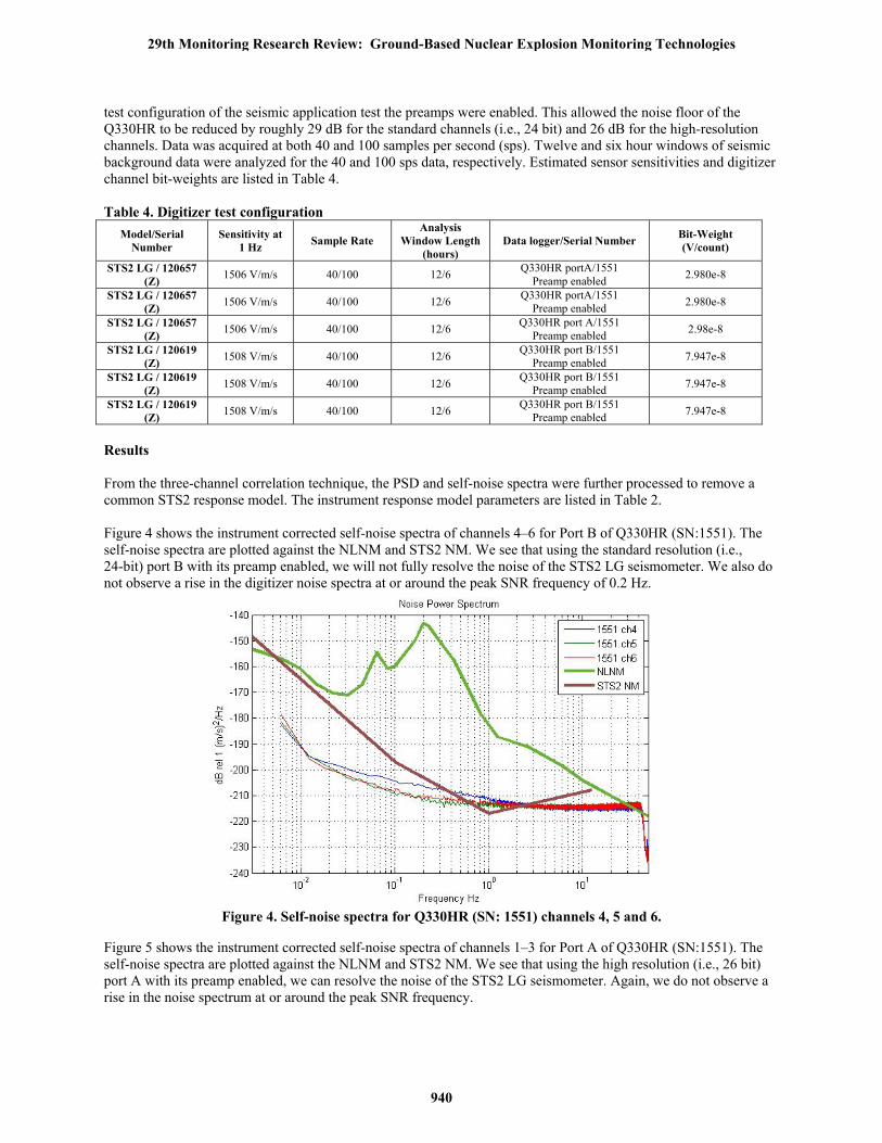
Results From the three-channel correlation technique, the PSD and self-noise spectra were further processed to remove a common STS2 response model. The instrument response model parameters are listed in Table 2. Figure 4 shows the instrument corrected self-noise spectra of channels 4–6 for Port B of Q330HR (SN:1551). The self-noise spectra are plotted against the NLNM and STS2 NM. We see that using the standard resolution (i.e., 24-bit) port B with its preamp enabled, we will not fully resolve the noise of the STS2 LG seismometer. We also do not observe a rise in the digitizer noise spectra at or around the peak SNR frequency of 0.2 Hz.

Figure 4. Self-noise spectra for Q330HR (SN: 1551) channels 4, 5 and 6.

Figure 5 shows the instrument corrected self-noise spectra of channels 1–3 for Port A of Q330HR (SN:1551). The self-noise spectra are plotted against the NLNM and STS2 NM. We see that using the high resolution (i.e., 26 bit) port A with its preamp enabled, we can resolve the noise of the STS2 LG seismometer. Again, we do not observe a rise in the noise spectrum at or around the peak SNR frequency.


940

Figure 5. Self-noise spectra for Q330HR (SN: 1551) channels 1, 2, and 3.

The RMS noise estimates, RMS full-scale and dynamic range of the six Q300HR channels tested are listed in Table 5. Using the STS2 low-gain noise model developed by Bob Hutt of the ASL, the MPDR was estimated to be –143.46 dB rel 1 (m/s)2/Hz. Comparing the dynamic range of the test sensors to the MPDR of the Hutt noise model shows the digitizer channels are –16.6 to–11.9 dB quieter than the STS2 low-gain theoretical noise model. Table 5. Results of DWR application test. RMS noise was computed between 0.01 and 16 Hz.

Serial Number Sample Rate RMS Noise (m/s)

RMS Full Scale (m/s)

Dynamic Range

Difference from MPDR of STS2 NM

120657-Z/1551 ch1 40 1.2618e-11 0.001274 –160.1 –16.6 120657-Z/1551 ch2 40 1.3035e-11 0.001274 –159.8 –16.3 120657-Z/1551 ch3 40 1.3381e-11 0.001274 –159.6 –16.1 120619-Z/1551 ch4 40/100 2.1774e-11 / 2.1880e-11 0.001274 –155.3 –11.9 120619-Z/1551 ch5 40/100 2.0389e-11 / 2.0434e-11 0.001274 –155.9 –12.5 120619-Z/1551 ch6 40/100 2.0489e-11 / 2.0490e-11 0.001274 –155.9 –12.4

Infrasound Application Test The goal of the infrasound application test was to determine the self-noise of three Chaparral Physics 2.5 (CP2.5) low-gain infrasound sensors and compare these noise estimates with an existing CP2.5 noise model developed by Whitaker and Kromer, 2003 and obtained through personal communication. One noteworthy point to make is the Whitaker and Kromer CP2.5 noise model may not be representative of the current Chaparral Physics product model 2.5, due to a change in manufacture location since 2003. This experiment was conducted in an underground testing vault at the Sandia FACT site, located near Albuquerque, NM. The data were acquired between 5/7/2007 and 5/8/2007 on a Geotech Smart24D data logger. Data were acquired at both 40 and 200 sps. Twelve and six hour windows were analyzed for the 40 and 200 sps data, respectively. More test configuration parameters are listed in Table 6. Two types of data were processed: white noise and acoustic background. A Wavetech 132-S817 signal generator was used to generate the white noise at approximately 40% of full-scale amplitude voltage. The white signal was input to a piston-phone, which converts the voltage signal to an acoustic signal. The generated acoustic signal has an equally distributed SNR, ~25–30 dB, across the application band of 0.1 to 8 Hz. The acoustic background data because of its variability were segmented into three groups based on increasing SNR levels low, medium, and high. The 12 hour total window was divided into three 3 hour windows for this comparison. By analysis of the data in this manner we can investigate sensor linearity in the presence of differing background signals.


941

Table 6. Infrasound application test configuration

Model/Serial Number

Sensitivity at 1 Hz

Sample Rate Analysis Window Length (hours)

Datalogger/Serial Number

RMS Full Scale (Pa)

Bit-Weight (V/count)

CP 2.5 – 061843 0.414 V/Pa 40/200 12/6 Smart24D/s1036 17.1 3.27e-7 CP 2.5 – 061845 0.409 V/Pa 40/200 12/6 Smart24D/s1036 17.3 3.27e-7 CP 2.5 - 061855 0.426 V/Pa 40/200 12/6 Smart24D/s1036 16.6 3.27e-7 Acoustic Background Test Results The three-sensor correlation technique was applied to acoustic background data of three differing levels. The resulting PSD and self-noise spectra were further processed to remove a common Chaparral 2.5 response model. The instrument response model parameters are listed in Table 7. Table 7. Infrasound application Chaparral 2.5 sensor response model Gain (V/Pa) 0.400 Zeros +/– 0.0 Poles (radian) –0.25 + j0.0 Figures 6a, b and c show the instrument corrected self-noise spectra of the three sensors tested for progressively increasing levels of acoustic background signal. For reference, the self-noise spectra are plotted against the Acoustic Low-Noise Model (ALNM), produced by Bowman et al, 2004 and the Chaparral 2.5 noise model of Whitaker and Kromer (personal communication). Figure 6a represents the low signal level, 6b the medium signal level, and 6c the high input signal level. The most notable feature between these results is the observation of an overall bias of the new Chaparral 2.5 sensors noise estimates versus the existing sensor noise model. The new sensor noise estimate appears to be 12–16 dB noisier than the existing model. The other notable observation is the sensor self-noise increases with increasing background signal level. Is this a non-linear effect of the sensor, or poor test design?

Figure 6a, b, c. Illustrations of infrasound sensors self-noise estimates with differing input signal levels for the

three sensors tested: SN 120619, 120621, and 80655. A nominal instrument response was removed from each spectrum, plotted against the SAIC ALNM and Chaparral 2.5 noise model of Whitaker and Kromer, 2003.


942

Using approximations of sensor sensitivities we compute the RMS full-scale pressure for each sensor. The RMS noise estimates were made for the frequency band of 0.1–8 Hz and the dynamic range was computed for each sensor and background signal level. The compiled results are in Table 8. For the three sensors tested the largest dynamic ranges were observed during low signal level background conditions. Table 8. Results of infrasound application test using acoustic background data. RMS noise was computed

between 0.1 and 8 Hz Serial Number Sample Rate RMS noise (Pa)

RMS Full Scale

(Pa) Dynamic Range

061843 – Low Noise 40 5.602e-4 17.1 -89.7 061843 – Med Noise 40 0.0020 17.1 -78.6 061843 – High Noise 40 0.0121 17.1 -63.0 061845 – Low Noise 40 3.406e-4 17.3 -94.1 061845 – Med Noise 40 0.0012 17.3 -83.2 061845 – High Noise 40 0.008 17.3 -66.7 061855 – Low Noise 40 4.409e-4 16.6 -91.5 061855 – Med Noise 40 0.0017 16.6 -79.8 061855 – High Noise 40 0.0120 16.6 -62.8

White Noise Test Results The three-sensor correlation technique was applied to acoustic white noise data. The resulting PSD and self-noise spectra were further processed to remove a common Chaparral 2.5 response model. The instrument response model parameters are listed in Table 6. Figure 7 shows the instrument corrected self-noise spectra of the three sensors tested using the white noise input signal. We again plot the self-noise spectra against the ALNM and the Chaparral 2.5 noise model of Whitaker and Kromer. We again observe an overall bias of the new Chaparral 2.5 sensor noise estimates versus the existing Chaparral 2.5 noise model. The sensor noise estimates appear to be 8–12 dB noisier than the existing model. Thus, we believe there might be a physical design change within the Chaparral 2.5 that warrants defining a new noise model for this specific sensor model.

Figure 7. Infrasound sensor self-noise spectra for white input signal.

Again, RMS noise estimates were made for the frequency band of 0.1–8 Hz and the dynamic range was computed for each sensor. The compiled results are in Table 9. For the three sensors tested the dynamic ranges were approximately the same as those observed for the low input signal level.


943

Table 9. Results of infrasound application test using white noise data. RMS noise was computed between 0.1 and 8 Hz

Serial Number Sample Rate

RMS Noise (Pa)

RMS Full Scale (m/s)

Dynamic Range

061843 40 4.130e-4 17.1 –92.3 061845 40 2.496e-4 17.3 –96.9 061855 40 4.607e-4 16.6 –91.1

CONCLUSIONS AND RECOMMENDATIONS

The new technique described by Sleeman, van Wettum, and Trampert (2006) for measuring the intrinsic noise spectra of seismic sensors relies on determining the mutual signal coherence among three similar, collocated instruments. Using this three sensor scheme, no assumptions must be made about individual sensor noise models. Testing this technique with synthetic data allowed us to explore several aspects of performance, most notably, correct extraction of coherent and incoherent noise levels. Secondly, this technique provides the ability to reliably estimate the internal noise spectra of similar sensors even in the presence of relatively high ambient background signals.

Proceeding into seismometer application testing, we noted close agreement with test sensor internal noise estimates and the STS2 NM, below 0.05 Hz and above 3 Hz. Between 0.05 and 3 Hz we believe that digitizer noise and non-linear sensor effects cause the differences observed between the STS2 NM and the internal seismometer noise estimates. Because of the observed microseism feature on the seismometer internal noise spectra, we explored using this technique to determine if the added noise was being added by the digitizer. Processing a common signal input recorded by three different digitizer channels allowed us to determine the digitizer self-noise for three channels. The results of this testing ruled out the digitizer as the cause of the microseism noise feature. Additional testing should allow us to fully resolve the STS2 low-gain noise model. We also recommend comparing these DWR channel noise estimates with Input Terminated Noise (ITN) Test data for these digitizers.

The technique was applied to three acoustic sensors, Chaparral model 2.5. Two types of acoustic data were processed: acoustic background and signal generated white noise. The acoustic background data allowed us to see how the sensors performed in the presence of differing input signal levels. We observed that the estimated internal sensor noise increased as the input signal level increased. Hence, the sensor’s dynamic range decreased as the input signal level increased. As a second point of comparison, white noise data produced RMS noise and dynamic range estimates that best matched those values obtained from the acoustic background test set with the lowest input signal level. We also observed that the existing Chaparral 2.5 noise model is 8–12 dB higher than current noise estimates and propose developing a new Chaparral 2.5 noise model based on current production line product. Further investigation should also be done to see if different input signal levels of white noise yield consistent noise estimates for sensors under test.

The other important results of the three-sensor correlation technique are the relative gain and phase estimates. Further work should also be done to explore the usefulness of the relative gain and phase for sensor response characterization or in basic sensor acceptance testing.

ACKNOWLEDGEMENTS

We would like to thank our colleagues at the USGS ASL for their cooperation in providing access to their test facility, and to C. R. Hutt at USGS ASL for the standard STS2 low-gain seismometer noise model.

REFERENCES

Bowman, R. J., G. E. Baker, and M. Bahavar (2004). Infrasound station ambient noise estimates, in Proceedings of the 26th Seismic Research Review: Trends in Nuclear Explosion Monitoring, LA-UR-04-5801, Vol. 1, pp. 608–617.

Holcomb, L.G. (1989). A direct method for calculating instrument noise levels in side-by-side seismometer evaluation, USGS Open-File Report 89-214.

Sleeman, R., A. van Wettum, and J. Trampert (2006). Three-channel correlation analysis: A new technique to measure instrumental noise of digitizers and seismic sensors, Bull. Seism. Soc Am. 96: 258–271.


944

seismic and infrasound sensor testing using three-channel

Documents