To appear in IPMI 2007.

Segmentation of Sub-Cortical Structures by theGraph-Shifts Algorithm

Jason J. Corso1, Zhuowen Tu1, Alan Yuille2, and Arthur Toga1

1 Center for Computational BiologyLaboratory of Neuro Imaging

2 Department of StatisticsUniversity of California, Los Angeles, USA

jcorso@ucla.edu

Abstract. We propose a novel algorithm called graph-shifts for performing im-age segmentation and labeling. This algorithm makes use of a dynamic hierar-chical representation of the image. This representation allows each iteration ofthe algorithm to make both small and large changes in the segmentation, similarto PDE and split-and-merge methods, respectively. In particular, at each iterationwe are able to rapidly compute and select the optimal change to be performed.We apply graph-shifts to the task of segmenting sub-cortical brain structures.First we formalize this task as energy function minimization where the energyterms are learned from a training set of labeled images. Then we apply the graph-shifts algorithm. We show that the labeling results are comparable in quantitativeaccuracy to other approaches but are obtained considerably faster: by orders ofmagnitude (roughly one minute). We also quantitatively demonstrate robustnessto initialization and avoidance of local minima in which conventional boundaryPDE methods fall.

1 IntroductionSegmenting an image into a number of labeled regions is a classic vision and medicalimaging problem, see [1,2,3,4,5,6] for an introduction to the enormous literature. Theproblem is typically formulated in terms of minimizing an energy function or, equiv-alently, maximizing a posterior probability distribution. In this paper, we deal with aspecial case where the number of labels is fixed. Our specific application is to segmentthe sub-cortical structures of the brain, see section (2). The contribution of this paper isto provide a novel algorithm called graph-shifts which is extremely fast and effectivefor sub-cortical segmentation.

A variety of algorithms, reviewed in section (2), have been proposed to solve theenergy minimization task for segmentation and labeling. For most of these algorithms,each iteration is restricted to small changes in the segmentation. For those methodswhich allow large changes, there is no procedure for rapidly calculating and selectingthe change that most decreases the energy.

Graph-shifts is a novel algorithm that builds a dynamic hierarchical representationof the image. This representation enables the algorithm to make large changes in thesegmentation which can be thought of as a combined split and merge (see [4] for recentwork on split and merge). Moreover, the graph-shifts algorithm is able to exploit thehierarchy to rapidly calculate and select the best change to make at each iteration. Thisgives an extremely fast algorithm which also has the ability to avoid local minima thatmight trap algorithms which rely on small local changes to the segmentation.

The hierarchy is structured as a set of nodes at a series of layers, see figure (1). Thenodes at the bottom layer form the image lattice. Each node is constrained to have asingle parent. All nodes are assigned a model label which is required to be the same as

m1

m1

m1 m1 m1

m1 m2

m2

m2

Initial State

m1

m1

m1

m2

m2

m2

m2

m2 m2

Shift 1

m1

m1

m1

m2

m2

m2

m2

m2m1

Shift 2

Fig. 1. Intuitive Graph-Shifts Example.

its parent’s label. There is a neighborhood structure defined atall layers of the graph. A graph shift alters the hierarchy bychanging the parent of a node, which alters the model label ofthe node and of all its descendants. This is illustrated in fig-ure (1), which shows three steps in a three layer graph coloringpotential shifts that would change the energy black and othersgray. The algorithm can be understood intuitively in terms ofcompeting crime families as portrayed in films like the Godfa-ther. There is a hierarchical organization where each node owesallegiance to its unique parent node (or boss) and, in turn, to itsboss’s boss. This gives families of nodes which share the sameallegiance (i.e. have the same model label). Each node has asubfamily of descendants. The top level nodes are the “bossesof all bosses” of the families. The graph-shifts algorithm pro-ceeds by selecting a node to switch allegiance (i.e. model label)to the boss of a neighboring node. This causes the subfamily ofthe node to also switch allegiance. The algorithm minimizes aglobal energy and at each iteration selects the change of alle-giance that maximally decreases the energy.

The structure of this paper is as follows. In section (2) wegive a brief background on segmentation. Section (3) describesthe graph-shifts algorithm for a general class of segmentationproblems. In section (4), we formulate the task of sub-corticallabeling in terms of energy function minimization and derive a graph-shifts algorithm.Section (5) gives experimental results and comparisons to other approaches.

2 BackgroundMany algorithms have been applied to segmentation, so we restrict our review to thosemethods most related to this paper. A common approach includes taking local gradientsof the energy function at the region boundaries and thereby moving the boundaries. Thisregion competition approach [2] can be successful when used with good initialization,but its local nature means that at each iteration step it can only make small changes tothe segmentation. This can cause slowness and also risks getting stuck in local min-ima. See [7] for similar types of partial differential equations (PDE) algorithms usinglevel sets and related methods. Graph cuts [3] is an alternative deterministic energyminimization algorithm that can take large leaps in the energy space, but it can onlybe applied to a restricted class of energy functions (and is only guaranteed to convergefor a subset of these) [8]. Simulated annealing [1] can in theory converge to the opti-mal solution of any energy function but, in practice, is extremely slow. The data-drivenMarkov chain Monte Carlo method [4] can combine classic methods, including splitand merge, to make large changes in the segmentation at each iteration, but remainscomparatively slow.

There have been surprisingly few attempts to define segmentation algorithms basedon dynamic hierarchical representations. But we are influenced by two recent papers.Segmentation by Weighted Aggregation (SWA) [9] is a remarkably fast algorithm thatbuilds a hierarchical representation of an image, but does not attempt to minimize aglobal energy function. Instead it outputs a hierarchy of segments which satisfy certainhomogeneity properties. Moreover, its hierarchy is fixed and not dynamic. The multi-

scale Swendson-Wang algorithm [10] does attempt to provide samples from a globalprobability distribution. But it has only limited hierarchy dynamics and its convergencerate is comparatively slow compared to SWA. A third related hierarchical segmentationapproach is proposed in [11], where a hyperstack, a Gaussian scale-space representationof the image, is used to perform a probabilistic linking (similar to region growing) ofvoxels and partial volumes in the scale-space. Finally, Tu [12] proposed a related seg-mentation algorithm that was similarly capable of making both small-scale boundaryadjustments and large-scale split-merge moves. In his approach, however, a fixed sizehierarchy is used, and the split-merge moves are attempted by a stochastic algorithm,which requires the evaluation of (often difficult to compute) proposal distributions.

Our application is the important task of sub-cortical segmentation from three-dimensional medical images. Recent work on this task includes [5,6,13,14,15,16]. Theseapproaches typically formulate the task in terms of probabilistic estimation or, equiva-lently, energy function minimization. The approaches differ by the form of the energyfunction that they use and the algorithm chosen to minimize it. The algorithms are usu-ally similar to those described above and suffer similar limitations in terms of conver-gence rates. In this paper, we will use a comparatively simple energy function similarto conditional random fields [17], where the energy terms are learned from trainingexamples by the probabilistic boosting tree (PBT) learning algorithm [18].

3 Graph-Shifts

This section describes the basic ideas of the graph-shifts algorithm. We first describethe class of energy models that it can be applied to in section (3.1). Next we describethe hierarchy in section (3.2), show how the energy can be computed recursively insection (3.3), and specify the general graph-shifts algorithm in section (3.4).

3.1 The Energy Models

The input image I is defined on a lattice D of pixels/voxels. For medical image ap-plications this is a three-dimensional lattice. The lattice has the standard neighborhoodstructure and we define the notation N(µ, ν) = 1 if µ ∈ D and ν ∈ D are neighborson the lattice, and N(µ, ν) = 0 otherwise. The task is to assign each voxel µ ∈ D toone of a fixed set of K models mµ ∈ {1, ...,K}. This assignment corresponds to asegmentation of the image into K, or more, connected regions.

We want the segmentation to minimize an energy function criterion:

E[{mω : ω ∈ D}] =∑ν∈D

E1(φ(I)(ν),mν) +12

∑ν∈D,µ∈D:N(ν,µ)=1

E2(I(ν), I(µ),mν ,mµ).

(1)In this paper, the second term E2 is chosen to be a boundary term that pays a penaltyonly for neighboring pixels/voxels which have different model labels (i.e.E2(I(ν), I(µ),mν ,mµ) = 0 if mν = mµ). This penalty can either be a penalty for thelength of the boundary, or may include a measure of the strength of local edge cues. Itincludes discretized versions of standard segmentation criteria such as boundary length∫

δRds and edge strength along boundary

∫δR|∇I|2ds. (Here s denotes arc length, R

denotes the regions with constant labels, and δR is their boundaries).

The first termE1 gives local evidence that the pixel µ takes modelmµ, where φ(I)(µ)denotes a nonlinear filter of the image evaluated at µ. In this paper, the nonlinear fil-ter will give local context information and will be learned from training samples, asdescribed in section (4.1). The model given in equation (1) includes a large class ofexisting models. It is restricted, however, by the requirement that the number of modelsis fixed and that the models have no unknown parameters.

3.2 The Hierarchy

We define a graph G to be a set of nodes µ ∈ U and a set of edges. The graph ishierarchical and composed of multiple layers. The nodes at the lowest layer are theelements of the lattice D and the edges are defined to link neighbors on the lattice. Thecoarser layers are computed recursively, as will be described in section (4.2). Two nodesat a coarse layer are joined by an edge if any of their children are joined by an edge.

The nodes are constrained to have a single parent (except for the nodes at the toplayer which have no parent) and every node has at least one child (except for nodes atthe bottom layer). We use the notation C(µ) for the children of µ, and A(µ) for theparent. A node µ on the bottom layer (i.e. on the lattice) has no children, and henceC(µ) = ∅. We use the notation N(µ, ν) = 1 to indicate that nodes µ, ν on the samelayer are neighbors, with N(µ, ν) = 0 otherwise.

At the top of the hierarchy, we define a special root layer of nodes comprised of asingle node for each of theK model labels. We write µk for these root nodes and use thenotation mµk

to denote the model variable associated with it. Each node is assigned alabel that is constrained to be the label of its parent. Since, by construction, all non-rootnodes can trace their ancestry back to a single root node, an instance of the graph G isequivalent to a labeled segmentation {mµ : µ ∈ D} of the image, see equation (1).

3.3 Recursive Computation of Energy

This section shows that we can decompose the energy into terms that can be assignedto each node of the hierarchy and computed recursively. This will be exploited in sec-tion (3.4) to enable us to rapidly compute the changes in energy caused by differentgraph shifts.

The energy function consists of regional and edge parts. These depend on the nodedescendants and, for the edge part, on the descendants of the neighbors. The regionalenergy E1 for assigning a model mµ to a node µ is defined recursively by:

E1(µ,mµ) =

E1 (φ(I)(µ),mµ) if C(µ) = ∅∑ν∈C(µ)

E1(ν,mµ) otherwise (2)

where E1 (φ(I)(µ),mµ) is the energy at the voxel from equation (1). The edge energyE2 between nodes µ1 and µ2, with models mµ1 and mµ2 is defined recursively by:

E2(µ1, µ2,mµ1 ,mµ2) =E2(I(µ1), I(µ2),mµ1 ,mµ2) if C(µ1) = C(µ2) = ∅∑ν1∈C(µ1), ν2∈C(µ2) :

N(ν1,ν2)=1

E2(ν1, ν2,mµ1 ,mµ2) otherwise (3)

where E2(I(µ1), I(µ2),mµ1 ,mµ2) is the edge energy for pixels/voxels in equation (1).The overall energy (1) was specified at the voxel layer, but it can be computed at any

layer of the hierarchy. For example, it can be computed at the top layer by:

E({mµk

: k = 1, ...,K})

=K∑

k=1

E1(µk,mµk) +

12

∑i,j:1,..,K

N(µi,µj)=1

E2(µi, µj ,mµi,mµj

).

(4)3.4 Graph-Shifts

The basic idea of the graph-shifts algorithm is to allow a node µ to change its parent tothe parent A(ν) of a neighboring node ν, as shown in figure (1). We will represent thisshift as µ→ ν.

This shift not have any effect on the labeling of nodes unless the new parent has adifferent label than the old one (i.e. when mA(µ) 6= mA(ν), or equivalently, mµ 6= mν).In this case, the change in parents will cause the node and its descendants to changetheir labels to that of the new parent. This will alter the labeling of the nodes on theimage lattice and hence will change the energy.

Consequently, we only need consider shifts between neighbors which have differentlabels. We can compute the changes in energy, or shift-gradient caused by these shiftsby using the energy functions assigned to the nodes, as described in section (3.3). Forexample, the shift from µ to ν corresponds to a shift-gradient ∆E(µ→ ν):

∆E(µ→ ν) = E1(µ,mν)− E1(µ,mµ) +∑η:N(µ,η)=1

[E2(µ, η,mν ,mη)− E2(µ, η,mµ,mη)] . (5)

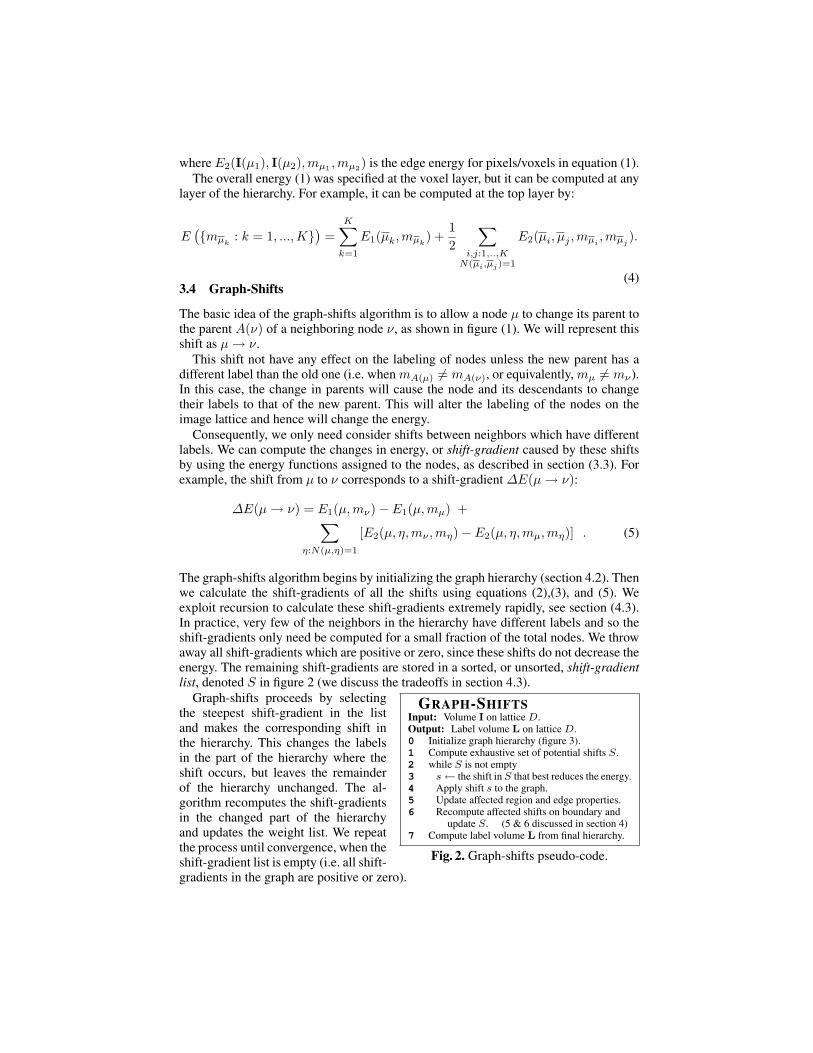
The graph-shifts algorithm begins by initializing the graph hierarchy (section 4.2). Thenwe calculate the shift-gradients of all the shifts using equations (2),(3), and (5). Weexploit recursion to calculate these shift-gradients extremely rapidly, see section (4.3).In practice, very few of the neighbors in the hierarchy have different labels and so theshift-gradients only need be computed for a small fraction of the total nodes. We throwaway all shift-gradients which are positive or zero, since these shifts do not decrease theenergy. The remaining shift-gradients are stored in a sorted, or unsorted, shift-gradientlist, denoted S in figure 2 (we discuss the tradeoffs in section 4.3).

GRAPH-SHIFTSInput: Volume I on lattice D.Output: Label volume L on lattice D.0 Initialize graph hierarchy (figure 3).1 Compute exhaustive set of potential shifts S.2 while S is not empty3 s← the shift in S that best reduces the energy.4 Apply shift s to the graph.5 Update affected region and edge properties.6 Recompute affected shifts on boundary and

update S. (5 & 6 discussed in section 4)7 Compute label volume L from final hierarchy.

Fig. 2. Graph-shifts pseudo-code.

Graph-shifts proceeds by selectingthe steepest shift-gradient in the listand makes the corresponding shift inthe hierarchy. This changes the labelsin the part of the hierarchy where theshift occurs, but leaves the remainderof the hierarchy unchanged. The al-gorithm recomputes the shift-gradientsin the changed part of the hierarchyand updates the weight list. We repeatthe process until convergence, when theshift-gradient list is empty (i.e. all shift-gradients in the graph are positive or zero).

Each shift is chosen to maximally decrease the energy, and so the algorithm is guar-anteed to converge to, at least, a local minimum of the energy function. The algorithmprefers to select shifts at the coarser layers of the hierarchy, because these typically alterthe labels of many nodes on the lattice and cause large changes in energy. These largechanges can ensure that the algorithm can escape from some bad local minima.

4 Segmentation of 3D Medical Images

Now we describe the specific application to sub-cortical structures. The specific energyfunction is given in section (4.1). Sections (4.2) and (4.3) describe the initialization andhow the shifts are computed and selected for the graph-shifts algorithm.

4.1 The Energy

Our implementation uses eight models for sub-cortical structures together with a back-ground model for everything else. The regional terms E1(µ,mµ) in the energy func-tion (1) contain local evidence that a voxel µ is assigned a labelmµ. This local evidencewill depend on a small region surrounding the voxel and hence is influenced by the lo-cal image context. We learn this local evidence from training data where the labeling isgiven by an expert.

We apply the probabilistic boosting tree (PBT) algorithm [18] to output a probabilitydistribution P (mµ|φ(I)(µ)) for the label mµ at voxel µ ∈ D conditioned on the re-sponse of a nonlinear filter φ(I)(µ). This filter depends on voxels within an 11×11×11window centered on µ, and hence takes local image context into account. The non-linearfilter φ is learned by the PBT algorithm which is an extension of the AdaBoost algo-rithm [19], [20]. PBT builds the filter φ(.) by combining a large number of elementaryimage features. These are selected from a set of 5,000 features which include Haar ba-sis functions and histograms of the intensity gradient. The features are combined usingweights which are also learned by the training algorithm.

We define the regional energy term by:

E1(µ,mµ) = − logP (mµ|φ(I)(µ)), (6)

which can be thought of as a pseudolikelihood approximation [18].The edge energy term can take two forms. We can use it to either penalize the length

of the segmentation boundaries, or to penalize the intensity edge strength along thesegmentation boundaries. This gives two alternatives:

E2(I(ν), I(µ),mν ,mµ) = 1− δmν ,mµ , (7)E2(I(ν), I(µ),mν ,mµ) = {1− δmν ,mµ}ψ(I(µ), I(ν)), . (8)

where ψ(I(µ), I(ν)) is a statistical likelihood measure of an edge between µ and ν; asimple example of such a measure is given in equation (9).

4.2 Initializing the Hierarchy

We propose a stochastic algorithm to quickly initialize the graph hierarchy that will beused during the graph shifts process. The algorithm recursively coarsens the graph byactivating some edges according to the intensity gradient in the volume and groupingthe resulting connected components up to a single node in the coarser graph layer. Thecoarsening procedure begins by defining a binary edge activation variable eµν on each

edge in the current graph layer Gt between neighboring nodes µ and ν (i.e., N(µ, ν) =1). The edge activation variables are then sampled according to

eµν ∼ γU({0, 1}) + (1− γ) exp [−α |I(µ)− I(ν)|] (9)

where U is the uniform distribution on the binary set and γ is a relative weight betweenU and the conventional edge gradient affinity (right-hand side).

After the edge activation variables are sampled, a connected components algorithmis used to form node-groups based on the edge activation variables. The size of a con-nected component is constrained by a threshold τ , which governs the relative degreeof coarsening between two graph layers. On the next graph layer, a node is created foreach component. Following, edges in the new graph layer are induced by the connectiv-ity on the current layer; i.e., two nodes in the coarse graph are connected if any two oftheir children are connected. The algorithm recursively executes this coarsening proce-dure until the size of the coarsened graph is within the range of the number of models,specified by a scalar β. Complete pseudo-code for this hierarchy initialization is givenin figure 3.

Let GT be the top layer of the graph hierarchy after initialization (example in fig-ure 3(b)). Then, we append a model layer GM on the hierarchy that contains a singlenode per model. Each node in GT becomes the child of the node in GM to which it hasbest fit, which is determined by evaluating the model fit P (m|µ) defined in section 4.1.One necessary constraint is that each node in GM has at least one child in GT , whichis enforced by first linking each node in GM to the node in GT with highest probabilityto its model and the remaining links are created as described earlier.

HIERARCHY INITIALIZATIONInput: Volume I on lattice D.Output: Graph hierarchy with layers G0, . . . , GT .0 Initialize graph G0 from lattice D.1 t← 0.2 repeat3 Sample edge activation variables in Gt using (9).4 Label every node in Gt as OPEN.5 while OPEN nodes remain in Gt.6 Create new, empty connected component C.7 Put a random OPEN node into queue Q.8 while Q is not empty and |C| < 1/τ .9 µ← removed head of Q.10 Add ν to Q, s.t. N(µ, ν) = 1 and eµν = 1.11 Add µ to C, label µ as CLOSED.12 Create Gt+1 with a node for each C.13 Define I(C) as mean intensity of its children.14 Inherit connectivity in Gt+1 from Gt.15 t← t + 1.16 until

˛Gt

˛< β ∗K.

(b) Example initialization. Top-left is coronal,top-right is sagittal, bottom-left is axial, andbottom-right is a 3D view.

Fig. 3. Initialization pseudo-code (left) and example (right).

4.3 Computing and Selecting Graph-ShiftsThe efficiency of the graph-shifts algorithm relies on fast computation of potential shiftsand fast selection of the optimal shift every iteration. We now describe how to satisfythese two requirements. To quickly compute potential shifts, we use an energy cachingstrategy that evaluates the recursive energy formulas (2) and (3) for the entire graph hi-erarchy following its creation (section 4.2). At each node, we evaluate and store the en-

ergies, denoted E1(µ,mµ) .= E1(µ,mµ) and E2(µ, ν,mµ,mν) .= E2(µ, ν,mµ,mν)for all µ, ν : N(µ, ν) = 1. These are quickly calculated in a recursive fashion. Thecomputational cost of initializing the energy cache is O(n log n).

Subsequently, we apply the cached energy to evaluate the shift-gradient (5) in theentire hierarchy; this computation is O(1) with the cache. At each node, we store theshift with the steepest gradient (largest negative ∆E), and discard any shift with non-negative gradient. The remaining shifts are stored in the potential shift list, denoted Sin figure 2. In the volumes we have been studying, this list is quite small: typically onlyabout 2% of all edges numbering about 60, 000 for volumes with 4 million voxels. Theentire initialization including caching energies in the whole hierarchy takes 10 – 15seconds on these volumes, which amounts to about 30% of the total execution time.

At step 3 in the graph-shifts algorithm (figure 2), we must find the optimal shift in thepotential shift list. One can use a sorted or unsorted list to store the potential shifts, withtradeoffs to both; an unsorted list requires no initial computation, no extra computationto add to the list, but anO(n) search at each iteration to find the best shift. The sorted listcarries an initial O(n log n) cost, an O(log n) cost for adding, but is O(1) for selectingthe optimal shift. Since every shift will cause modifications to the potential shift list,and the size of the list decreases with time (as fewer potential shifts exist), we chooseto store an unsorted list and expend the linear search at each iteration.

As the graph shifts are applied, it is necessary to dynamically keep the hierarchy insynch with the energy landscape. Recomputing the entire energy cache and potentialshift set is prohibitively expensive. Fortunately, it is not necessary: by construction, ashift is a very local change to the solution and only affects nodes along the boundaryof the recently shifted subgraph. The number of affected nodes is dependent on thenode connectivity and the height of the graph (it is O(log n)); the node connectivity isrelatively small and constant since the coarsening is roughly isotropic, and the heightof the graph is logarithmic in the number of input voxels.

First, we update the energy cache associated with each affected node. This amountsto propagating the energy change up the graph to the roots. Let µ→ ν be the executedshift. The region energy update must remove the energy contribution to A(µ) and addit to A(ν), which is the new parent of µ after the shift. The update rule is

E1(A(µ),mµ))′ = E1(A(µ),mµ)− E1(µ,mµ) (10)

E1(A(ν),mν))′ = E1(A(ν),mν) + E1(µ,mν) , (11)

and it must be applied recursively to each parent until the root layer. Due to limitedspace, we do not discuss the details of the similar but more complicated procedure toupdate the edge energy cache terms E2. Both procedures are also O(log n).

Second, we update the potential shifts given the change in the hierarchy. All nodesalong the shift boundary both below and above the shift layer must be updated becausethe change in the energy could result in changes to the shift-gradients, new potentialshifts, and expired potential shifts (between two now nodes with the same model). Gen-erally, this remains a small set since the shifts are local moves. As before, at each ofthese nodes, we compute and store the shift with the steepest negative gradient usingthe cached energies and discard any shift with a non-negative gradient or between twonodes with the same model. There are O(log n) affected shifts.

Shift 5 Shift 50 Shift 500 Shift 5000Fig. 4. Example of the graph-shifts process sampled during the minimization. Coronal and sagittal planes areshown, top and bottom respectively.

0 1000 2000 3000 4000 50000

200

400

600

800

1000

1200

Shift Number

Shif

t Mas

s

0 1000 2000 3000 4000 50000

1

2

3

4

Shift Number

Shif

t Lay

er

0 1000 2000 3000 4000 50000

0.2

0.4

0.6

0.8

1

Shift Number

Cum

ulat

ive

Shif

t Gra

dien

t Fra

ctio

n

(a) (b) (c)

Fig. 5. (a) Graph shows the number of voxels (mass) that are moved per shift for 5000 shifts. (b) Graph showsthe level in the hierarchy at which at shift occurs. (c) Graph shows the cumulative fraction of the total energyreduction that each shift effects.

5 Experimental ResultsA dataset of 28 high-resolution 3D SPGR T1-weighted MR images was acquired ona GE Signa 1.5T scanner as series of 124 contiguous 1.5 mm coronal slices (256x256matrix; 20cm FOV). Brain volumes were roughly aligned and linearly scaled to perform9 parameter registration. Four control points were manually given to perform this globalregistration. Expert neuro-anatomists manually labeled each volume into the followingsub-cortical structures: hippocampus (LH, RH for left and right, resp. shown in greenin figures), caudate (LC, RC in blue), putamen (LP, RP in purple), and ventricles (LV,RV, in red). We arbitrarily split the dataset in half and use 14 subjects for training and14 for testing. The training volumes are used to learn the PBT region models and theboundary presence models. During the hierarchy initialization, we set the τ parameterto 0.15. We experimented with different values for τ , and found that varying it does notgreatly affect the segmentation result.

The graph-shifts algorithm is very fast. We show an example process in figure 4 (thisis the same volume as in figure 3(b)). Initialization, including the computation of theinitial potential shift set, takes about 15 seconds. The remaining part of the graph shiftsnormally takes another 35 seconds to converge on a standard Linux PC workstation(2GB memory, 3Ghz cpu). Convergence occurs when no potential energy-reducing shiftremains. Our speed is orders of magnitude faster than reported estimates on 3D medicalsegmentation: Yang et al. [13] is 120 minutes, FreeSurfer [5] is 30 minutes, RegionCompetition (PDE, obtained from a local implementation) is 5 minutes.

In figure 5-(c), we show the cumulative weight percentage of the same sequenceof graph-shifts as figure 4. Here, we see that about 75% of the total energy reductionoccurs within the first 1000 graph shifts. This large, early energy reduction corresponds

Table 1. Segmentation accuracy using volume and surface measurements. A comparison to theFreeSurfer method run on the same data is included for the volume measurements in table 2.

Training Set Testing SetLH RH LC RC LP RP LV RV LH RH LC RC LP RP LV RV

Prec. 82% 70% 86% 86% 77% 81% 86% 86% 80% 58% 82% 84% 74% 74% 85% 85%Rec. 60% 58% 82% 78% 72% 72% 88% 87% 61% 49% 81% 76% 67% 68% 87% 86%

Haus. 11.4 21.6 10.1 11.7 14.7 11.6 26.9 19.0 17.1 26.8 10.4 10.1 15.7 13.7 20.8 21.5Mean 1.6 4.0 1.1 1.1 2.3 1.8 1.0 0.8 1.8 7.6 1.2 1.2 2.7 2.5 0.9 0.9Med. 1.1 3.1 1.0 1.0 1.4 1.2 0.4 0.3 1.1 6.9 1.0 1.0 1.6 1.6 0.4 0.5

to the shifts that occur at high layers in the hierarchy and have large masses as depictedin figure 5-(a) and (b). The mass of a shift is the number of voxels that are relabeledas a result of the operation. Yet, it is also clear from the plots that the graph-shiftsat all levels at considered throughout the minimization process; recall, at any giventime the potential shift list stores all energy reducing shifts and chooses the best one.Considering the majority of the energy reduction happens in the early stages of thegraph-shift process, it is possible to stop the algorithm early when the shift gradientdrops below a certain threshold.

0 2000 4000 6000 8000 10000Shift Number

Tot

al E

nerg

y

Graph−ShiftsPDE

Fig. 6. Total energy reduction comparison ofgraph-shifts to a PDE method.

In figure 6, we compare the total energy re-duction of the dynamic hierarchical graph-shiftsalgorithm to the more conventional PDE-typeenergy minimization approach. To keep a faircomparison, we use the same structure and ini-tial conditions in both cases. However, to ap-proximate a PDE-type approach, we restrict thegraph shifts to occur across single voxel bound-aries (at the lowest layer in the hierarchy) only.As expected, the large-mass moves effect an ex-ponential decrease in energy while the decreasefrom the single voxel moves is roughly linear.

To quantify the accuracy of the segmentation, we use the standard volume (precisionand recall), and surface distance (Hausdorff, mean and median) measurements. Theseare presented in table 1; in each case, the average over the set is given. In these exper-iments, we weighted the unary term four times as strong as the binary term; the powerof the discriminative, context-sensitive models takes the majority of the energy whilethe binary term enforces local continuity and smoothness. Our accuracy is comparable

Table 2. FreeSurfer [5] accuracy.LH RH LC RC LP RP LV RV

Prec. 48% 51% 77% 78% 70% 76% 81% 69%Rec. 67% 75% 78% 76% 83% 83% 76% 71%

Haus. 25.3 11.5 23.0 26.1 13.1 10.8 31.9 51.8Mean 3.9 2.1 1.9 2.0 1.8 1.4 1.8 9.6Med. 2.1 1.5 1.0 1.0 1.3 1.0 0.9 3.9

or superior to the current state of theart in sub-cortical segmentation. To makea quantitative comparison, we computedthe same scores using the FreeSurfer [5]method on the same data (results in ta-ble 2). We show a visual example of thesegmentation in figure 7.

Next, we show the graph-shifts algorithm is robust to initialization. We systemati-cally perturbed the initial hierarchy by taking random shifts with positive gradient toincrease the energy by 50%. Then, we started the graph-shifts from the degraded ini-tial condition. In all cases, graph-shifts converged to (roughly) the same minimum; toquantify it, we calculated the standard deviation (SD) of the precision + recall score

Graph-Shifts Manual

Fig. 7. An example of the sub-cortical structure segmentation result using the graph-shifts algorithm.

for over 100 instances. For all structures the SD is very small: LH: 0.0040, RH: 0.0011,LC: 0.0009, RC: 0.0013, LP: 0.0014, RP: 0.0013, LV: 0.0009, RV: 0.0014.

1

2Truth Init GS PDE

Fig. 8. Graph-shifts (GS) can avoid local min-ima. See text for details.

We now show that the large shifts providedby the hierarchical representation help avoid lo-cal minima in which PDE methods fall. We cre-ated a synthetic test image containing three sep-arate i.i.d. Gaussian-distributed brightness mod-els (depicted as red, green, and blue regions infigure 8). Following a similar perturbation as de-scribed above, we ran the graph-shifts algorithmas well as a PDE algorithm to compute the seg-

mentation and reach a minimum. As expected, the graph-shifts method successfullyavoids local minima that the PDE method falls into; in figure 8, we show two suchcases. In the figure, the left column shows the input image and true labeling; the nextthree columns show the initial state, the graph-shifts result and the PDE result for twocases (rows 1 and 2).

6 ConclusionWe proposed graph-shifts, a novel energy minimization algorithm that manipulates adynamic hierarchical decomposition of the image volume to rapidly and robustly mini-mize an energy function. We defined the class of energy functions it can minimize, andderived the recursive energy on the hierarchy. We discussed how the energy functionscan include terms that are learned from labeled training data. The dynamic hierarchicalrepresentation makes it possible to make both large and small changes to the segmen-tation in a single operation, and the energy caching approach provides a deterministicway to rapidly compute and select the optimal move at each iteration.

We applied graph-shifts to the segmentation of sub-cortical brain structures in high-resolution MR 3D volumes. The quantified accuracy for both volume and surface dis-tances is comparable or superior to the state-of-the-art for this problem, and the algo-rithm converges orders of magnitude faster than conventional minimization methods(about a minute). We demonstrated quantitative robustness to initialization and avoid-ance of local minima in which local boundary methods (e.g., PDE) fell.

In this paper, we considered the class of energies which used fixed model terms thatwere learned from training data. We are currently exploring extensions to the graph-

shifts algorithm that would update the model parameters during the minimization. Tofurther improve sub-cortical segmentation, we are investigating a more sophisticatedshape model as well as additional sub-cortical structures. Finally, we are conductingmore comprehensive experiments using a larger dataset and cross-validation.

AcknowledgementsThis work was funded by the National Institutes of Health through the NIH Roadmapfor Medical Research, Grant U54 RR021813 entitled Center for Computational Biology(CCB). Information on the National Centers for Biomedical Computing can be obtainedfrom http://nihroadmap.nih.gov/bioinformatics.

References1. Geman, S., Geman, D.: Stochastic Relaxation, Gibbs Distributions, and Bayesian Restora-

tion of Images. IEEE Trans. on Pattern Analysis and Machine Intelligence 6 (1984) 721–7412. Zhu, S.C., Yuille, A.: Region Competition. IEEE Trans. on Pattern Analysis and Machine

Intelligence 18(9) (1996) 884–9003. Boykov, Y., Veksler, O., Zabih, R.: Fast Approximate Energy Minimization via Graph Cuts.

IEEE Trans. on Pattern Analysis and Machine Intelligence 23(11) (2001) 1222–12394. Tu, Z., Zhu, S.C.: Image Segmentation by Data-Driven Markov Chain Monte Carlo. IEEE

Trans. on Pattern Analysis and Machine Intelligence 24(5) (2002) 657–6735. Fischl, B., Salat, D.H., et al.: Whole brain segmentation: Automated labeling of neu-

roanatomical structures in the human brain. Neuron 33 (2002) 341–3556. Pohl, K.M., Fisher, J., Kikinis, R., Grimson, W.E.L., Wells, W.M.: A Bayesian Model for

Joint Segmentation and Registration. NeuroImage 31 (2006) 228–2397. Chan, T.F., Shen, J.: Image Processing and Analysis: Variational, PDE, Wavelet, and

Stochastic Methods. Soc. for Industrial and Applied Mathematics (SIAM), Phil., PA (2005)8. Kolmogorov, V., Zabih, R.: What Energy Functions Can Be Minimized via Graph Cuts? In:

European Conference on Computer Vision. Volume 3. (2002) 65–819. Sharon, E., Brandt, A., Basri, R.: Fast Multiscale Image Segmentation. In: IEEE Conf. on

Computer Vision and Pattern Recognition. Volume I. (2000) 70–7710. Barbu, A., Zhu, S.C.: Multigrid and Multi-level Swendsen-Wang Cuts for Hierarchic Graph

Partitions. In: IEEE Computer Vision and Pattern Recognition. Volume 2. (2004) 731–73811. Vincken, K., Koster, A., Viergever, M.A.: Probabilistic Multiscale Image Segmentation.

IEEE Trans. on Pattern Analysis and Machine Intelligence 19(2) (1997) 109–12012. Tu, Z.: An Integrated Framework for Image Segmentation and Perceptual Grouping. In:

International Conference on Computer Vision. (2005)13. Yang, J., Staib, L.H., Duncan, J.S.: Neighbor-Constrained Segmentation with Level Set

Based 3D Deformable Models. IEEE Trans. on Medical Imaging 23(8) (2004)14. Pizer, S.M., Fletcher, P.T., et al.: Deformable m-reps for 3d medical image segmentation.

International Journal of Computer Vision 55 (2003) 85–10615. Cocosco, C., Zijdenbos, A., Evans, A.: A Fully Automatic and Robust Brain MRI Tissue

Classification Method. Medical Image Analysis 7 (2003) 513–52716. Wyatt, P.P., Noble, J.A.: MAP MRF joint segmentation and registration. In: Conference on

Medical Image Computing and Computer-Assisted Intervention. (2002) 580–58717. Lafferty, J., McCallum, A., Pereira, F.: Conditional Random Fields: Probabilistic Models for

Segmenting and Labeling Sequence Data. In: Int. Conference on Machine Learning. (2001)18. Tu, Z.: Probabilistic Boosting-Tree: Learning Discriminative Models for Classification,

Recognition, and Clustering. In: International Conference on Computer Vision. (2005)19. Freund, Y., Schapire, R.E.: A Decision-Theoretic Generalization of On-line Learning and an

Application to Boosting. Journal of Computer and System Science 55(1) (1997) 119–13920. Schapire, R.E., Singer, Y.: Improved Boosting Algorithms Using Confidence-Rated Predic-

tions. Machine Learning 37(3) (1999) 297–336