sector magnets or transverse electromagnetic fields in
TRANSCRIPT

Sector magnets or transverse electromagnetic fieldsin cylindrical coordinates
T. Zolkin*
Fermilab, P.O. Box 500, Batavia, Illinois 60510-5011, USA(Received 9 March 2016; published 10 April 2017)
Laplace’s equation is considered for scalar and vector potentials describing electric or magnetic fields incylindrical coordinates, with invariance along the azimuthal coordinate. A series of special functions arefound which, when expanded to lowest order in power series in radial and vertical coordinates, replicateharmonic polynomials in two variables. These functions are based on radial harmonics found by Edwin M.McMillan forty years ago. In addition to McMillan’s harmonics, a second family of radial harmonics isintroduced to provide a symmetric description between electric and magnetic fields and to describe fieldsand potentials in terms of the same functions. Formulas are provided which relate any transverse fieldsspecified by the coefficients in the power series expansion in radial or vertical planes in cylindricalcoordinates with the set of new functions. This result is important for potential theory and for theoreticalstudy, design and proper modeling of sector dipoles, combined function dipoles and any general sectorelement for accelerator physics. All results are presented in connection with these problems.
DOI: 10.1103/PhysRevAccelBeams.20.043501
I. INTRODUCTION
The description of sector magnets, any curved magnetsymmetric along its azimuthal cylindrical coordinate (longi-tudinal coordinate in accelerator physics) is an importantissue. Every modern accelerator code includes such ele-ments, themost important being combined function dipoles.A widely used method, which goes back to Karl Brown’s1968 paper [1], is based on a solution of Laplace’s equationfor a scalar potential using a power series in cylindricalcoordinates. A similar approach applied to Laplace’s equa-tion for the longitudinal component of a vector potentialcan be found for example in [2]. The same approach appearsin more recent books, e.g. in great detail in [3].Two major bottlenecks should be noticed. First, if one
looks for a solution in the form of a series, then these seriesmust be truncated. In our case truncation means thatpotentials no longer satisfy Laplace’s equation. (Of coursepotentials can “satisfy” Laplace’s equation up to anydesired order by keeping more and more terms in theexpansion.) More importantly, the recurrence equation isundetermined. In every new order of recurrence one has toassign an arbitrary constant, which will affect all otherhigher order terms. This ambiguity leads to the fact thatthere is no preferred, unique choice of basis functions; itmakes it difficult to compare accelerator codes, since
different assumptions might be used for representationsof basis functions.This indeterminacy has a simple geometrical illustration.
Looking for a field with a pure normal dipole componenton a circular equilibrium orbit in lowest order, one cancome up with an almost arbitrary shape of the magnet’snorth pole if its south pole is symmetric with respect to themidplane. In the case of a dipole, the series can be truncatedby keeping only its dipole component. For higher ordermultipoles in cylindrical coordinates truncation withoutviolation of Laplace’s equation is not possible.While working on an implementation of sector magnets
for Synergia, I found assumptions which let me sum seriesfor pure electric and magnetic skew and normal multipoles.Looking further for symmetry in the description allowedme to generate a family of solutions in which all the seriescould be summed, so that no truncation was required.While discussing my results with Sergei Nagaitsev, hebrought my attention to an article by McMillan written in1975 [4]. As I found later, the same result was independ-ently obtained by Mane and published in the same journalabout 20 years later [5] without citing McMillan’s originalwork. It made me want to write this article in order to bringattention back to these forgotten results.Joiningmy results toMcMillan’s, I would like to present a
new representation for multipole expansions in cylindricalcoordinates. Any transverse field can be expanded in termsof these functions and related to power series expansionsin horizontal or vertical planes. The new approach does notcontradict previous results but embraces them. The ambi-guity in choice of coefficients and the problem of truncationare resolved. Thus it can be employed for theoretical studies,design and simulation of sector magnets.
Published by the American Physical Society under the terms ofthe Creative Commons Attribution 4.0 International license.Further distribution of this work must maintain attribution tothe author(s) and the published article’s title, journal citation,and DOI.
PHYSICAL REVIEW ACCELERATORS AND BEAMS 20, 043501 (2017)
2469-9888=17=20(4)=043501(18) 043501-1 Published by the American Physical Society

The paper is structured as follows. Section II providesthe expansion of fields in multipoles for cases with zero andconstant curvatures. The connection between this approachand Taylor expansion is provided at the end of this section.Appendices A and B describe global and curvilinearFrenet-Serret coordinate systems including general equa-tions of motion for a particle in it. The case of puretransverse electric or magnetic fields is described inSecs. B 1 and B 2. Appendix C contains the main differ-ential relations used in this article. Finally, Appendixes D–Fare supplementary materials with harmonics, fields, poten-tials and Taylor series.
II. EXPANSION OF TRANSVERSEELECTROMAGNETIC FIELDS
In appendixes A and B we provided dynamical equationsof motion without specifying how to represent electromag-netic fields. In the next two subsections we will discuss themultipole field expansion for the two most important typesof elements: R-element for κ ¼ 0 and S-element defined forκ ¼ const ¼ 1=R0, see Fig. 1.“R-” stands for “rectangular.” This element is the one
with ðq1; q2; q3Þ simply being a right-handed Cartesiancoordinate system, which we will denote as ðx; y; zÞ. Fieldsin such elements are invariant along the z axis, and theelements usually serve as quadrupoles, sextupoles, octu-poles or combined function correctors. In addition one candesign pure R-dipoles, while combined function bending
magnets are exotic and very complicated since the equi-librium orbit will not coincide with the axis of symmetry.S-element is the element defined with the natural sector
coordinate system. Defining the set of normalized coor-dinates (x ¼ q1=R0, y ¼ q2=R0, z ¼ q3=R0), one can seethat it simply can be related to normalized right-handedcylindrical coordinates (ρ ¼ 1þ x, y, θ ¼ z=R0) and thusall fields are invariant along azimuthal coordinate θ.S-elements are suitable for the design of combined functionbending magnets, since in contrast to R-elements, theequilibrium orbit follows along θ.
A. Multipoles in Cartesian coordinates
In Cartesian coordinates, Laplace’s equations for trans-verse electro- and magnetostatic fields are in the same formwhich significantly simplifies the problem:
Δ⊥Φ ¼ ∂2Φ∂x2 þ ∂2Φ
∂y2 ¼ 0;
Δ⊥A ¼�∂2Az
∂x2 þ ∂2Az
∂y2�ez ¼ 0:
Introduction of complex variables allows a very compactdescription of this problem with a unified description ofelectric and magnetic fields [6]. Suppose we have a hol-omorphic function of complex variable Z ¼ xþ iy, whichwe will call a complex scalar potential, whose real part isdefined to be the longitudinal component of avector potentialand whose imaginary part is the electric scalar potential,
ΩðZÞ ¼ Azðx; yÞ þ iΦðx; yÞ:Since the real and imaginary parts of any holomorphicfunction are harmonic functions, Az and Φ automaticallysatisfy Laplace’s equation. Indeed, supposewe have a vectorfield F ¼ ðFx; FyÞ. Introducing the Wirtinger derivatives,
∂∂Z ¼ 1
2
� ∂∂x − i
∂∂y
�and
∂∂Z ¼ 1
2
� ∂∂xþ i
∂∂y
�;
one can write
∂Ω∂Z ¼ 0;
∂Ω∂Z ¼ FðZÞ;
where the first equation is the Cauchy-Riemann conditionfor Ω, which guarantees that this field can be implementedvia either magnetic or electric potentials:
Fx ¼ −∂Φ∂x ¼ ∂Az
∂y ;
Fy ¼ −∂Φ∂y ¼ −
∂Az
∂x :
q2= y R0
q1= x R0
q3= z R0
q2= y
q1= x
q3= z
n
tbFrenet−Serretframe
Equilibriumorbit
coordinatesGlobal
Cylindricalcoordinates
R ,0ρ = 1,x = 0
θ = z
y
bt
ρ = 1 + x
nS−element
R−element
FIG. 1. Illustration of R- and S-elements. Elements are shownin brown. Global curvilinear coordinates with associated gridlines are shown in black. Black dashed line represents anequilibrium orbit. An example of the Frenet-Serret frame attachedto an equilibrium orbit is drawn in blue colors. For S-element, anadditional right-handed normalized cylindrical system is addedand shown in cyan.
T. ZOLKIN PHYS. REV. ACCEL. BEAMS 20, 043501 (2017)
043501-2

The second equation defines the complex function of fieldcomponents such that
Fx ¼ −ℑFðZÞ and Fy ¼ −ℜFðZÞ;which all together are equivalent to F ¼ −∇Φ ¼ ∇ ×A.The complex function FðZÞ is the holomorphic functionagain and the Cauchy-Riemann equation gives
∂F∂Z ¼ 0;
which asserts that field F is irrotational and divergence freewhich is equivalent to time-independent free of electriccharge and current density Maxwell’s equations
∇ · F ¼ 0 and ∇ × F ¼ 0:
For accelerator physics purposes the expansion of fieldsusually represented in terms of homogeneous harmonicpolynomials of two variables, which are defined throughthe complex power function,
Anðx; yÞ ¼ ℜZn ¼ 1
2½ðxþ iyÞn þ ðx − iyÞn�
¼Xnk¼0
�n
k
�xn−kyk cos
kπ2;
Bnðx; yÞ ¼ ℑZn ¼ 1
2i½ðxþ iyÞn − ðx − iyÞn�
¼Xnk¼0
�n
k
�xn−kyk sin
kπ2:
Explicit expressions are well known and up to tenth orderare listed in Table VII of Appendix D. These functionssatisfy the transverse Laplace’s equation and are related toeach other through the Cauchy-Riemann equation as
∂An
∂x ¼ ∂Bn
∂y and∂An
∂y ¼ −∂Bn
∂x :
In addition one can introduce “ladder-like” lowering andraising integro-differential operators which relate functionsof different order to each other:
nðA;BÞn−1 ¼∂∂x ðA;BÞn ¼ � ∂
∂y ðB;AÞn
and
ðA;BÞn ¼ nZ
x
0
dxðA;BÞn−1 þ ynðcos; sinÞ nπ2
with A0 ¼ 1 and B0 ¼ 0.Thus one can define two independent sets of solutions:
normal (sometimes called upright or straight) and skewpure multipoles, which we will denote with overline ð…Þ
TABLE I. Formulas for the scalar potential, longitudinalcomponent of the vector potential and field components for purenormal and skew 2n-poles in Cartesian coordinates.
Normal Skew
ΦðnÞ ¼ −CnBnn! ΦðnÞ ¼ −Cn
Ann!
AðnÞz ¼ −Cn
Ann! AðnÞ
z ¼ CnBnn!
FðnÞx ¼ Cn
Bn−1ðn−1Þ! FðnÞ
x ¼ CnAn−1ðn−1Þ!
FðnÞy ¼ Cn
An−1ðn−1Þ! FðnÞ
y ¼ −CnBn−1ðn−1Þ!
FIG. 2. Normal and skew 2n-pole magnets in Cartesian coordinates. Each figure shows magnetic (electric) field streamlines and poles’shape in transverse cross section. North (positive electrostatic potential) and south (negative electrostatic potential) poles are shown inred and blue and are given by ðB;AÞn ¼∓ Rn
p respectively, where Rp is the distance to the pole’s tip.
SECTOR MAGNETS OR TRANSVERSE … PHYS. REV. ACCEL. BEAMS 20, 043501 (2017)
043501-3

and underline ð…Þ respectively. The complex scalar poten-tials of pure multipoles are
ΩðnÞ ¼ −CnZn
n!and ΩðnÞ ¼ −iCn
Zn
n!;
where Cn and Cn are coefficients determining the strengthof magnets. Corresponding vector fields are defined to haveodd and even midplane symmetries:
FðnÞy ðx; yÞ ¼ FðnÞ
y ðx;−yÞ and FðnÞx ðx; 0Þ ¼ 0;
FðnÞx ðx; yÞ ¼ FðnÞ
x ðx;−yÞ and FðnÞy ðx; 0Þ ¼ 0:
Formulas for potentials and fields are listed in Table I andexact expressions are provided in Appendix E. Figure 2shows the cross section of idealized multipole magnets.
B. Multipoles in cylindrical coordinates
In the normalized right-handed cylindrical coordinatesystem, when cylindrical symmetry (∂=∂θ ¼ 0) isimposed, the Laplace’s equations reduce to
Δ↷Φ ¼ Δ⊥Φþ 1
ρ
∂Φ∂ρ
¼ ∂2Φ∂ρ2 þ 1
ρ
∂Φ∂ρ þ ∂2Φ
∂y2 ¼ 0;
Δ↷A ¼�Δ↷Aθ −
Aθ
ρ2
�eθ
¼�∂2Aθ
∂ρ2 þ 1
ρ
∂Aθ
∂ρ þ ∂2Aθ
∂y2 −Aθ
ρ2
�eθ ¼ 0:
Compared to the case with Cartesian coordinates theseequations look quite different from each other. In order toretain the symmetry one can note that
ðΔ↷AÞθ ¼1
ρ
� ∂2
∂ρ2 −1
ρ
∂∂ρþ
∂2
∂y2�ðρAθÞ:
Thus looking for the solution in a form similar to harmonichomogeneous polynomials
Φ ¼ −Xnk¼0
F n−kðρÞðn − kÞ!
yk
k!
�Cn sin
kπ2þ Cn cos
kπ2
�;
Aθ ¼ −Xnk¼0
1
ρ
Gn−kðρÞðn − kÞ!
yk
k!
�Cn cos
kπ2− Cn sin
kπ2
�;
where F nðρÞ and GnðρÞ are the functions to be determined,one can find two recurrence equations:
∂2F nðρÞ∂ρ2 þ 1
ρ
∂F nðρÞ∂ρ ¼ nðn − 1ÞF n−2ðρÞ;
∂2GnðρÞ∂ρ2 −
1
ρ
∂GnðρÞ∂ρ ¼ nðn − 1ÞGn−2ðρÞ:
F n and Gn are related to each other through
Gn−1 ¼1
nρ∂F n
∂ρ and F n−1 ¼1
n1
ρ
∂Gn
∂ρ :
This allows us to construct lowering operators,
F n ¼1
ðnþ 1Þðnþ 2Þ�1
ρ
∂∂ρ
�ρ∂∂ρ
��F nþ2;
Gn ¼1
ðnþ 1Þðnþ 2Þ�ρ∂∂ρ
�1
ρ
∂∂ρ
��Gnþ2;
and corresponding raising operators
F n ¼ nðn − 1ÞZ
ρ
1
1
ρ
Zρ
1
ρF n−2dρdρ;
Gn ¼ nðn − 1ÞZ
ρ
1
ρ
Zρ
1
1
ρGn−2dρdρ;
where the lower limits take care of two arbitrary constantsof integration. These operators can be used to recursivelycalculate all members of F - and G-functions. An additionalconstraint to terminate recurrences defines lowest ordersn ¼ 0, 1 as
F 0¼ 1; F 1¼ lnρ; G0¼ 1; G1¼ðρ2−1Þ=2:The first ten members of F n and Gn are listed in Tables II
and III and are shown in Fig. 3; in Appendix F one can findTaylor series of these functions at ρ ¼ 1. The differencerelation for F n including first members has been found byEdwin M. McMillan and I would like to acknowledge hisresult by giving them a name ofMcMillan radial harmonics.In addition to his results, adjoint McMillan radial harmon-ics, Gn, are introduced in order to provide the symmetry inthe description between electric and magnetic fields.Finally, in order to define the set of functions for pure
S-multipoles (Table IV) we will define sector harmonics:
AðeÞn ðρ; yÞ ¼
Xnk¼0
�n
k
�F n−kðρÞyk cos
kπ2;
AðmÞn ðρ; yÞ ¼
Xnk¼0
�n
k
�Gn−kðρÞ
ρyk cos
kπ2;
BðeÞn ðρ; yÞ ¼
Xnk¼0
�n
k
�F n−kðρÞyk sin
kπ2;
BðmÞn ðρ; yÞ ¼
Xnk¼0
�n
k
�Gn−kðρÞ
ρyk sin
kπ2;
obeying the differential relations
nðA;BÞðeÞn−1 ¼ � ∂ðB;AÞðeÞn
∂y ¼ 1
ρ
∂ðρðA;BÞðmÞn Þ
∂ρ ;
nðA;BÞðmÞn−1 ¼ � 1
ρ
∂ðρ ðB;AÞðmÞn Þ
∂y ¼ ∂ðA;BÞðeÞn
∂ρ :
Figure 4 shows the cross section of idealized magneticmultipoles poles and their corresponding fields. The first
T. ZOLKIN PHYS. REV. ACCEL. BEAMS 20, 043501 (2017)
043501-4

FIG. 3. First five even (top row) and odd (bottom row) members of regular polynomials Pn ¼ ρn, F nðρÞ, GnðρÞρ and GnðρÞ functions
from the left to the right, respectively.
TABLE II. First ten members of F -functions.
n F nðρÞ0 11 ln ρ2 1
2ðρ2 − 1Þ − ln ρ
3 32½−ðρ2 − 1Þ þ ðρ2 þ 1Þ ln ρ�
4 3½18ðρ4 − 1Þ þ 1
2ðρ2 − 1Þ − ðρ2 þ 1
2Þ ln ρ�
5 152½− 3
8ðρ4 − 1Þ þ ð1
4ρ4 þ ρ2 þ 1
4Þ ln ρ�
6 454½ 136ðρ6 − 1Þ þ 1
2ðρ4 − 1Þ − 1
4ðρ2 − 1Þ − ð1
2ρ4 þ ρ2 þ 1
6Þ ln ρ�
7 31516
½− 1154ðρ6 − 1Þ − 1
2ρ2ðρ2 − 1Þ þ f1
9ðρ6 þ 1Þ þ ρ2ðρ2 þ 1Þg ln ρ�
8 1054½ 196ðρ8 − 1Þ þ 4
9ðρ6 − 1Þ þ 3
8ðρ4 − 1Þ − 2
3ðρ2 − 1Þ − ð1
3ρ6 þ 3
2ρ4 þ ρ2 þ 1
12Þ ln ρ�
9 3158½− 25
192ðρ8 − 1Þ − 5
6ρ2ðρ4 − 1Þ þ f 1
16þ ρ2ðρ2
2þ 1Þð1
8ρ4 þ 7
4ρ2 þ 1Þg ln ρ�
TABLE III. First ten members of G-functions.
n GnðρÞ0 11 1
2ðρ2 − 1Þ
2 1½− 12ðρ2 − 1Þ þ ρ2 ln ρ�
3 32½14ðρ4 − 1Þ − ρ2 ln ρ�
4 3½− 58ðρ4 − 1Þ þ 1
2ðρ2 − 1Þ þ ρ2ðρ2
2þ 1Þ ln ρ�
5 154½ 112ðρ6 − 1Þ þ 3
4ρ2ðρ2 − 1Þ − ρ2ðρ2 þ 1Þ ln ρ�
6 458½− 5
9ðρ6 − 1Þ − 1
2ðρ4 − 1Þ þ ðρ2 − 1Þ þ ρ2ð1
3ρ4 þ 2ρ2 þ 1Þ ln ρ�
7 10516
½ 124ðρ8 − 1Þ þ 7
6ρ2ðρ4 − 1Þ − ðρ6 þ 3ρ4 þ ρ2Þ ln ρ�
8 354½− 47
96ðρ8 − 1Þ − 2ðρ6 − 1Þ þ 9
8ðρ4 − 1Þ þ 4
3ðρ2 − 1Þ þ ρ2ð1
4ρ6 þ 3ρ4 þ 9
2ρ2 þ 1Þ ln ρ�
9 31532
½ 140ðρ10 − 1Þ þ 35
24ρ2ðρ6 − 1Þ þ 5
2ρ4ðρ2 − 1Þ − ðρ8 þ 6ρ6 þ 6ρ4 þ ρ2Þ ln ρ�
SECTOR MAGNETS OR TRANSVERSE … PHYS. REV. ACCEL. BEAMS 20, 043501 (2017)
043501-5

FIG. 4. Normal and skew 2n-pole magnets in cylindrical coordinates. Each figure shows magnetic (electric) field streamlinesand poles’ shape in the transverse cross section. North (positive electrostatic potential) and south (negative electrostatic potential)
poles are shown in red and blue and given by constant levels of ðB;AÞðeÞn ¼∓ const respectively, const ¼ 1 for this example.The bottom plot shows 3D models of sector magnets with θ ¼ 3π=2: normal and skew S-dipoles, normal and skew S-quadrupoles and skew S-sextupole from the left to the right and the top to the bottom respectively. The equilibrium orbit isshown in green color.
T. ZOLKIN PHYS. REV. ACCEL. BEAMS 20, 043501 (2017)
043501-6

six members of sector harmonics are listed in Table VIII ofAppendix D and exact expressions for potentials and fieldsin Appendix E.Finally, one can relate experimental data on the power
series expansions of the fields at the reference orbit:
Fx;yjx¼0¼ Fx;yjeq þ
y1!
∂Fx;y
∂y����eqþ y2
2!
∂2Fx;y
∂y2����eqþ � � �
or
Fx;yjy¼0¼ Fx;yjeq þ
x1!
∂Fx;y
∂x����eqþ x2
2!
∂2Fx;y
∂x2����eqþ � � �
to strength coefficients, which allows the expansion of ageneral S-element in terms of harmonics (see Table V).
C. Recurrence equations in sector coordinates
An alternative approach to finding expansions forpotentials is to use a power series ansatz. In Cartesiancoordinates the use of
Φ ¼ −X∞m;n≥0
Vm;nxm
m!
yn
n!
gives the recurrence relation
Vmþ2;n þ Vm;nþ2 ¼ 0:
This equation immediately defines all coefficients. It is easyto see that, up to a common factor, the solutions coincidewith harmonic homogeneous polynomials ðA;BÞn.In sector coordinates, the same substitution forΦ and the
substitution
Aθ ¼ −X∞m;n≥0
1
1þ xVm;n
xm
m!
yn
n!
for the longitudinal component of the vector potential givestwo new recurrences, respectively:
TABLE IV. Formulas for the scalar potential, azimuthal com-ponent of the vector potential and field components for “pure”normal and skew 2n-poles in cylindrical coordinates.
Normal Skew
ΦðnÞ ¼ −CnBðeÞnn! ΦðnÞ ¼ −Cn
AðeÞnn!
AðnÞθ ¼ −Cn
AðmÞnn! AðnÞ
θ ¼ CnBðmÞnn!
FðnÞρ ¼ Cn
BðmÞn−1
ðn−1Þ! FðnÞρ ¼ Cn
AðmÞn−1
ðn−1Þ!
FðnÞy ¼ Cn
AðeÞn−1
ðn−1Þ! FðnÞy ¼ −Cn
BðeÞn−1
ðn−1Þ!
TABLE V. Relationship between coefficients determining the strength of pure normal and skew S-multipoles and power seriesexpansion of field in radial and vertical planes on equilibrium orbit.
n x ¼ 0 y ¼ 0
Cn 1 Fy Fy
2 ∂yFx ∂xFy
3 −∂2yFy ∂2
xFy þ ∂xFy
4 −∂3yFx ∂3
xFy þ ∂2xFy − ∂xFy
5 ∂4yFy ∂4
xFy þ 2∂3xFy − ∂2
xFy þ ∂xFy
6 ∂5yFx ∂5
xFy þ 2∂4xFy − 3∂3
xFy þ 3∂2xFy − 3∂xFy
7 −∂6yFy ∂6
xFy þ 3∂5xFy − 3∂4
xFy þ 6∂3xFy − 9∂2
xFy þ 9∂xFy
8 −∂7yFx ∂7
xFy þ 3∂6xFy − 6∂5
xFy þ 12∂4xFy − 27∂3
xFy þ 45∂2xFy − 45∂xFy
9 ∂8yFy ∂8
xFy þ 4∂7xFy − 6∂6
xFy þ 18∂5xFy − 51∂4
xFy þ 126∂3xFy − 225∂2
xFy þ 225∂xFy
Cn 1 Fx Fx
2 −∂yFy ∂xFx þ Fx
3 −∂2yFx ∂2
xFx þ ∂xFx − Fx
4 ∂3yFy ∂3
xFx þ 2∂2xFx − ∂xFx þ Fx
5 ∂4yFx ∂4
xFx þ 2∂3xFx − 3∂2
xFx þ 3∂xFx − 3Fx
6 −∂5yFy ∂5
xFx þ 3∂4xFx − 3∂3
xFx þ 6∂2xFx − 9∂xFx þ 9Fx
7 −∂6yFx ∂6
xFx þ 3∂5xFx − 6∂4
xFx þ 12∂3xFx − 27∂2
xFx þ 45∂xFx − 45Fx
8 ∂7yFy ∂7
xFx þ 4∂6xFx − 6∂5
xFx þ 18∂4xFx − 51∂3
xFx þ 126∂2xFx − 225∂xFx þ 225Fx
9 ∂8yFx ∂8
xFx þ 4∂7xFx − 10∂6
xFx þ 30∂5xFx − 105∂4
xFx þ 330∂3xFx − 855∂2
xFx þ 1575∂xFx − 1575Fx
SECTOR MAGNETS OR TRANSVERSE … PHYS. REV. ACCEL. BEAMS 20, 043501 (2017)
043501-7

Vmþ2;n þ Vm;nþ2 ¼ −ðm� 1ÞVmþ1.n −mVm−1;nþ2:
The detailed approach on how to treat these equationscan be found for example in [3]. In order to solve theserecurrences, one can look for a solution where each termcan be expressed in the form
Vi;j ¼ V�i;j þ Vðiþj−1Þ
i;j þ Vðiþj−2Þi;j þ Vðiþj−3Þ
i;j þ � � � ;
where starred variables are the “design” terms given bypure multipole fields and thus satisfying
V�mþ2;n þ V�
m;nþ2 ≡ 0:
Other coefficients VðkÞi;j are terms induced by lower kth order
pure multipoles due to recurrence. Thus, in order to findan expression for a particular 2n-pole we will start therecurrence from the nth order assuming that
Vn;0 ¼ −Vn−2;2 ¼ � � � or Vn−1;1 ¼ −Vn−3;3 ¼ � � �
for normal and skew elements. Then wewill start exploiting
the recurrence where all terms in the form VðnÞi;j for
iþ j > n are subject to be determined.This approach has two major disadvantages. First, in
order to use the result, one will have to truncate arecurrence. As a result the potentials representing magnetsno longer satisfy Laplace’s equation. This violates the“physics” and should be avoided. While potentials can beapproximated with any precision by keeping an appro-priate number of terms, there is another issue. Whensolving the recurrence, at each new order one will findthat an arbitrary constant αi ∈ ð0; 1Þ should be introducedsince the system is undetermined. An additionalassumption, ðAs;ΦÞjx¼0 ∝ yn, allows us to terminate orsum the series. The resulting solutions would then coincidewith the ones obtained above.
III. SUMMARY
The scalar and vector Laplace’s equations for statictransverse electromagnetic fields in curvilinear orthogo-nal coordinates with zero and constant curvature aresolved. In Cartesian coordinates these solutions are well-known harmonic polynomials in two variables. The setof solutions in cylindrical coordinates, named sectorharmonics, should not be confused with cylindricalharmonics where ρ-dependent terms are given byBessel functions (which occasionally are also calledcylindrical harmonics). In contrast, the radial part isgiven by a set of harmonics, independently introducedby Edwin M. McMillan in a “forgotten” article, andadjoint radial harmonics described in this work (in
addition it was rediscovered by Mane in the beginningof the 1990s). When expanded around a circular designorbit, the sector harmonics resemble the solutions inCartesian geometry. This set of functions has two majoradvantages over the traditional approach, widely used inthe accelerator community, of using recurrences based ona power series ansatz. They do not require truncation andsatisfy Laplace’s equation exactly, and they provide awell-defined full basis of functions which can be relatedto any field by expansion in radial or vertical planes, seeTable V. Including the model Hamiltonians for t- and s-representations, where no assumptions but the fieldsymmetry has been used, one can construct a numericalscheme to integrate the equations of motion. Thus, Iwould like to suggest the set of sector harmonics as anew basis for the description and design of sectormagnets with translational symmetry along the azimuthalcoordinate.
ACKNOWLEDGMENTS
The author would like to thank Leo Michelotti, EricStern and James Amundson for their discussions andvaluable input, Alexey Burov for encouraging me to finda full family of solutions, Valeri Lebedev whose solutionfor electrostatic quadrupole led me to a generalization,just as was the case with Edwin M. McMillan and F.Krienen, and Sergei Nagaitsev who introduced me toMcMillan’s article, which helped me with the symmetricdescription of electromagnetic fields. FermiLab is operatedby Fermi Research Alliance, LLC under Contract No. De-AC02-07CH11359 with the U.S. Department of Energy.
APPENDIX A: GENERAL EQUATIONSOF MOTION IN GLOBAL LAB FRAME
The Lagrangian of a relativistic particle of mass m withan electric charge e in most general static electromagneticfield is given by
L½R; _R; t� ¼ −mc2
γðVÞ − eΦðRÞ þ e(V ·AðRÞ);
where R ¼ ðQ1; Q2; Q3Þ is a position vector in the con-figuration space of coordinates spanned by a right-handedCartesian coordinate system, fE1; E2; E3g, V ¼ dR=dt≡_R is a vector of matching generalized velocities, ΦðRÞ andAðRÞ are the electric scalar and magnetic vector potentialsrespectively, and
γðVÞ ¼ 1ffiffiffiffiffiffiffiffiffiffiffiffiffiffiffiffiffiffiffiffi1 − βðVÞ2
pis the relativistic Lorentz factor, with βðVÞ ¼ jVj=c.Substituting the Lagrangian into the Euler-Lagrange
equations (Lagrange’s equations of the second kind)
T. ZOLKIN PHYS. REV. ACCEL. BEAMS 20, 043501 (2017)
043501-8

ddt
∂L∂ _R
−∂L∂R ¼ 0
with shorthand notation
∂∂a ¼
� ∂∂a1 ;
∂∂a2 ;
∂∂a3
�
representing a vector of partial derivatives with respect tothe indicated variables, gives the equation of motion whichis the relativistic form of the Lorentz force
F ¼ e½Eþ ðV × BÞ�
or explicitly
ddtðγm _QiÞ ¼ eðEi þ ϵijk _QjBkÞ:
Electric and magnetic fields are related to the scalar electricand vector magnetic potentials through the usual gradientand curl operators:
E ¼ ðE1; E2; E3Þ≡ −∇Φ;
B ¼ ðB1; B2; B3Þ≡∇ ×A:
The corresponding Hamiltonian formulation employsphase space coordinates ðP;QÞ, where P is the particle’scanonical (total) momentum,
P≡ ∂L∂ _R
¼ Πþ eA
with Π ¼ γmV being the particle’s kinematic momentum.The Hamiltonian might be constructed using the Legendretransformation of L:
H½P;Q; t� ¼ V · P − L ¼X3i¼1
_QiPi − L
¼ cffiffiffiffiffiffiffiffiffiffiffiffiffiffiffiffiffiffiffiffiffiffiffiffiffiffiffiffiffiffiffiffiffiffiffiffim2c2 þ ðP − eAÞ2
qþ eΦ:
The time evolution of the system is given by Hamilton’sequations
dPdt
¼ −∂H∂Q and
dQdt
¼ ∂H∂P
or equivalently
_Q ¼ cP − eAffiffiffiffiffiffiffiffiffiffiffiffiffiffiffiffiffiffiffiffiffiffiffiffiffiffiffiffiffiffiffiffiffiffiffiffi
m2c2 þ ðP − eAÞ2p ;
_P ¼ eð∇AÞ · _Q − e∇Φ:
APPENDIX B: GLOBAL COORDINATESASSOCIATED WITH FRENET-SERRET FRAME
The model of accelerator assumes the specification of areference orbit designed for a particle with certain equi-librium energy and assignment of beam line elementsplaced along it. In the case of a circular accelerator theclosed orbit of a machine with alignment errors in generalwill not coincide with reference orbit. For most acceleratorneeds (except e.g. helical orbits for muon cooling) thedesigned orbit is piecewise flat function, which means thatit consists of a series of curves with zero torsion; moreover,usually, these curves are straight lines and circular arcs. Inorder to better exploit the geometry of beam motion andsymmetry of electromagnetic fields we will introduce thelocal Frenet-Serret frame attached to the equilibrium orbitand new global coordinates associated with it (see Fig. 5).
Q1
Q1 Q
1
Q3
Q2
Q2
Q3
Q3
Q2
Q1
Q2
Q3
t
n
b
t
b
b
n
t
n
nb
t
FIG. 5. Schematic plot of a reference orbit for an acceleratorconsisting of five straight and five 72° curved sections. Lab frameand local Frenet-Serret frames are shown in black and blue colorsrespectively. The test particle winding the equilibrium orbit isshown in red.
t
Q
Q1
Q
R(s)
b
r(s)
3
2 R (s)0
n
FIG. 6. Illustration of a test particle’s position vectorexpressed as a transverse, i.e. for fixed q3, displacement fromequilibrium orbit.
SECTOR MAGNETS OR TRANSVERSE … PHYS. REV. ACCEL. BEAMS 20, 043501 (2017)
043501-9

We identify a particular curve segment in space asthe local “reference path” (See Fig. 6). A particle whoseorbit would follow that curve perfectly is a “referenceparticle” and its orbit, the “reference orbit.” LetR0ðtÞ be itsposition vector as a function of time. Arclength along thepath can be expressed as
sðtÞ ¼Z
t
0
j _R0ðtÞjdt;
andR0 can be parametrized as a function of s rather than t.The local Frenet-Serret coordinate frame with origin at R0
has right-handed orthonormal basis vectors, fn; b; tg (orTNB frame), defined as follows: (i) tangent unit vector
t ¼ dR0ðsÞds
;
(ii) outward-pointing normal unit vector
n ¼ −1
κðsÞdtds
;
(iii) and binormal unit vector
b ¼ t × n;
where κ ¼ jdt=dsj defines the local curvature of theequilibrium orbit. Using the Frenet-Serret formulasdescribing the derivatives of unit vectors in terms of eachother,
d
264t
n
b
375 ¼
2640 −κ 0
κ 0 τ
0 −τ 0
375264t
n
b
375ds;
where τðsÞ is the torsion of an equilibrium orbit whichmeasures the failure of a curve to be planar, the positionvector of a test particle and its infinitesimal can beexpressed as a displacement from an equilibrium orbit,
R ¼ R0ðsÞ þ rðsÞ ¼ R0ðsÞ þ q1nþ q2b
dR ¼ ndq1 þ bdq2 þ ð1þ κq1Þtdq3 þ τðq1b − q2nÞdq3;where ðq1; q2; q3Þ are local curvilinear coordinates spannedon ðn; b; tÞ. One can see that in the case of flat orbit, i.e.τ ¼ 0, the local Frenet-Serret frame can be associated withglobal orthogonal coordinate system with a line element ina form
dl ¼ h1e1dq1 þ h1e1dq1 þ h1e1dq1;
where scale factors are h1¼ h2¼ 1 and h≡ h3 ¼ 1þ κq1.The use of global coordinates with the metric provided
by the local Frenet-Serret frame allows one to write theLagrangian as
L½r; _r; t� ¼ −mc2
ffiffiffiffiffiffiffiffiffiffiffiffiffi1 −
v2
c2
s− eΦþ ev ·A;
where v ¼ ð _q1; _q2; h _q3Þ is the particle’s velocity expressedin new coordinates. Thus the equation of motion is
ddtðγmvÞ ¼ eðEþ ϵijkeivjBkÞ þ γm _q23K;
where the vector in the right-hand side of the equation isdefined as
K ¼ ðκh; 0; κ0q1Þ;
and κ0 ≡ dκ=dq3 is the derivative of κ with respect to thelongitudinal coordinate. Derivatives of potentials usingexpressions for differential operators in curvilinear orthogo-nal coordinates form Table VI. Calculating components ofthe new canonical momenta
pi
hi≡ 1
hi
∂L∂ _qi ¼ γmvi þ eAiðrÞ
allows one to rewrite the Hamiltonian
H½p;q; t� ¼ c
ffiffiffiffiffiffiffiffiffiffiffiffiffiffiffiffiffiffiffiffiffiffiffiffiffiffiffiffiffiffiffiffiffiffiffiffiffiffiffiffiffiffiffiffiffiffiffiffiffiffiffiffiffim2c2 þ
X3i¼1
�pi − ehiAi
hi
�2
vuut þ eΦ
and equations of motion
_qi×hi¼c2
H−eΦpi−ehiAi
hi;
_pi=hi¼c2
H−eΦ
�eϵijk
pj
hjBkþ
Ki
h2
�p3−ehA3
h
�2�þeEi:
Further simplifications can be made by specifying atype of the field or a certain symmetry. We will restrictourself to the case of transverse electromagnetic fields.In orthogonal curvilinear coordinate system associatedwith Serret-Frenet frame these are the fields with trans-lation symmetry along longitudinal coordinate q3. Thus,the scalar and vector potentials are a function of trans-verse coordinates only and we shall assume the vectorpotential has only one nonvanishing component which isA3. Taken together, these imply the gauge condition,∇ ·A ¼ 0. Both scalar and vector potentials satisfyLaplace’s equation,
ΔΦ ¼ 1
h
� ∂∂q1
�h∂Φ∂q1
�þ ∂∂q2
�h∂Φ∂q2
��¼ 0;
ΔA ¼ ∂∂q1
�1
h∂ðhA3Þ∂q1
�þ ∂∂q2
�1
h∂ðhA3Þ∂q2
�¼ 0:
T. ZOLKIN PHYS. REV. ACCEL. BEAMS 20, 043501 (2017)
043501-10

The corresponding fields are given by Maxwell equations
E ¼ −∇Φ; B ¼ ∇ ×A; ri
E1 ¼ −∂Φ∂q1 ; B1 ¼
1
h∂ðhA3Þ∂q2 ;
E2 ¼ −∂Φ∂q2 ; B2 ¼ −
1
h∂ðhA3Þ∂q1 ;
with differential operators defined for the orthogonal curvi-linear coordinate system (see Table VI in Appendix C).In the case of pure electric or magnetic fields further
simplifications can be applied. For numerical integrationpurposes, it is convenient to have a Hamiltonian in theform of a sum of “kinetic” and “potential” energies, so thatpotentials will be separated from momentum coordinates.In this case, one can easily construct a symplectic integratorconsisting of “drifts” and “kicks” associated with kineticand potential terms respectively (e.g. [7]). Depending onthe field type two models can be employed.
1. t-representation
For a pure electric field, when the curvature is constant(dκ=ds ¼ 0), not only the Hamiltonian but also p3 is aninvariant of motion, and the problem is essentially twodimensional. Measuring time in units of ct and normalizingthe transverse momenta by the longitudinal component,~p1;2 ¼ p1;2=p3, one has
H½ ~p;q; ct� ¼ 1
h
ffiffiffiffiffiffiffiffiffiffiffiffiffiffiffiffiffiffiffiffiffiffiffiffiffiffiffiffiffiffiffiffiffiffiffiffiffiffiffiffiffiffiffiffiffiffiffiffiffiffiffiffiffiffiffip23 þ h2m2c2
p23
þ h2ð ~p21 þ ~p2
2Þs
þ ep3c
Φ:
We will call this model Hamiltonian the t-representation;with no assumptions made, but the field symmetry, wederived general equations of motion which can be used forthe basis for the construction of the symplectic integrator.In a paraxial approximation, ~p1;2 ≪ 1, and for p1;2 ≫ mcthe form is significantly simpler, and a limit of straightcoordinates when h ¼ 1 is obvious:
H½ ~p;q; ct� ≈ h
�~p21
2þ ~p2
2
2
�þ 1
hþ ep3c
Φ:
2. s-representation
For a pure magnetic field the Hamiltonian is harder toexploit since it has only a square root and thus no terms tosplit. Introducing an extended Hamiltonian with a newfictitious orbit (“time”) parameter, τ, where the old inde-pendent variable and old Hamiltonian with a negative signwill be treated as an additional pair of canonically con-jugated coordinates, ð−H; tÞ, one has
0≡O½p1; p2; p3;−H;q1; q2; q3; t; τ�
¼ c
ffiffiffiffiffiffiffiffiffiffiffiffiffiffiffiffiffiffiffiffiffiffiffiffiffiffiffiffiffiffiffiffiffiffiffiffiffiffiffiffiffiffiffiffiffiffiffiffiffiffiffiffiffiffiffiffiffiffiffiffiffiffiffiffiffiffiffim2c2 þ p2
1 þ p22 þ
�p3 − ehA3
h
�2
s−H:
Integration of the additional equations of motion gives
H is invariant; and t ¼ τ þ C0:
We can set the arbitrary constant of integration, C0 ¼ 0.Continuing to assume that the curvature is constant, as
was done in the case of an electric field, the longitudinalcomponent of momentum is conserved. We shall use −p3
as a new Hamiltonian, reducing the number of degrees offreedom back to 3 by using q3 as a new independentvariable:
−p3 ≡K½p1; p2;−H;q1; q2; t; q3�
¼ −h
ffiffiffiffiffiffiffiffiffiffiffiffiffiffiffiffiffiffiffiffiffiffiffiffiffiffiffiffiffiffiffiffiffiffiffiffiffiffiffiffiffiffiffiffiffiffiffiffiffi�Hc
�2
−m2c2 − p21 − p2
2
s− ehA3:
The use of generating function
G2ðt;−ΠÞ ¼ −tffiffiffiffiffiffiffiffiffiffiffiffiffiffiffiffiffiffiffiffiffiffiffiffiffiffiffiffiffiffiΠ2c2 þ ðmc2Þ2
qwill allow one to use the full kinetic momentum −Π of aparticle instead of −H as one of canonical momentums:
K½p1; p2;−Π; q1; q2; l; q3� ¼ −hffiffiffiffiffiffiffiffiffiffiffiffiffiffiffiffiffiffiffiffiffiffiffiffiffiffiΠ2 − p2
1 − p22
q− ehA3;
where corresponding canonical coordinate is a particle’straversed path l ¼ −∂G2=∂Π ¼ βct.Since the Hamiltonian does not explicitly depend on l,
the full momentum Π is conserved and we can excludeassociated degrees of freedom using the further renormal-ization of the Hamiltonian K → K≡K=Π, which canbe achieved by renormalizing transverse components ofcanonical momentums p1;2 → ~p1;2 ¼ p1;2=Π:
−p3
Π≡ K½ ~p1; ~p2; q1; q2; q3�
¼ −hffiffiffiffiffiffiffiffiffiffiffiffiffiffiffiffiffiffiffiffiffiffiffi1 − ~p2
1 − ~p22
q−
eΠhA3:
We will call this model Hamiltonian s-representationsince the longitudinal coordinate (sometimes referred toas the natural parameter along equilibrium orbit, s) isused as a time parameter. This representation is conven-ient to use for the numerical integrator construction fortransverse magnetic fields. The paraxial approximation,~p1;2 ≪ 1, gives
K½ ~p;q; q3� ≈ h
�~p21
2þ ~p2
2
2
�− h −
eΠhA3:
SECTOR MAGNETS OR TRANSVERSE … PHYS. REV. ACCEL. BEAMS 20, 043501 (2017)
043501-11

APPENDIX C: DIFFERENTIAL OPERATORS IN ORTHOGONAL COORDINATES
Differential operators in orthogonal curvilinear coordinates are listed in Table VI.
APPENDIX D: HOMOGENEOUS AND SECTOR HARMONICS
Harmonic homogeneous polynomials and sector harmonics are listed below in Tables VII and VIII respectively.
TABLE VI. Differential operators in general orthogonal coordinates ðq1; q2; q3Þ whereH ¼ h1h2h3, and its expressions in orthogonalcoordinates associated with Serret-Frenet frame.
Operation Notation Expression
Gradient ∇ϕP
3k¼1
1hk
∂ϕ∂qk ek
∂ϕ∂q1 e1 þ
∂ϕ∂q2 e2 þ 1
h∂ϕ∂q3 e3
Divergence ∇ · FP
3k¼1
1H
∂∂qk ðHhk FkÞ
1h ½∂ðhF1Þ∂q1 þ ∂ðhF2Þ∂q2 þ ∂F3∂q3 �
Curl ∇ × F P3k¼1
hk ekH ϵijk
∂∂qi ðhjFjÞ
1h ½∂ðhF3Þ∂q2 − ∂F2∂q3 �e1 þ 1
h ½∂F1∂q3 −∂ðhF3Þ∂q1 �e2 þ ½∂F2∂q1 −
∂F1∂q2 �e3Scalar Laplacian Δϕ ¼ ∇ · ð∇ϕÞ P
3k¼1
1H
∂∂qk ðHh2k
∂ϕ∂qkÞ
1h ½ ∂
∂q1 ðh∂ϕ∂q1Þ þ ∂
∂q2 ðh∂ϕ∂q2Þ þ ∂
∂q3 ð1h∂ϕ∂q3Þ�
Vector Laplacian △F ¼ ∇ð∇ · FÞ −∇ × ð∇ × FÞ P3k¼1 f 1
hk∂∂qk ½ 1H ∂
∂qi ðHhi FiÞ� − hkH ϵijk
∂∂qi ½
h2jH ϵlmj
∂∂ql ðhmFmÞ�gek
TABLE VII. Harmonic homogeneous polynomials in two variables.
n An Bn
0 1 01 x y2 x2 − y2 2xy
3 x3 − 3xy2 3x2y − y3
4 x4 − 6x2y2 þ y4 4x3y − 4xy3
5 x5 − 10x3y2 þ 5xy4 5x4y − 10x2y3 þ y5
6 x6 − 15x4y2 þ 15x2y4 − y6 6x5y − 20x3y3 þ 6xy5
7 x7 − 21x5y2 þ 35x3y4 − 7xy6 7x6y − 35x4y3 þ 21x2y5 − y7
8 x8 − 28x6y2 þ 70x5y4 − 84x3y6 þ 9xy8 8x7y − 56x5y3 þ 56x3y5 − 8xy7
9 x9 − 36x7y2 þ 126x5y4 − 84x3y6 þ 9xy8 9x8y − 84x6y3 þ 126x4y5 − 36x2y7 þ y9
T. ZOLKIN PHYS. REV. ACCEL. BEAMS 20, 043501 (2017)
043501-12
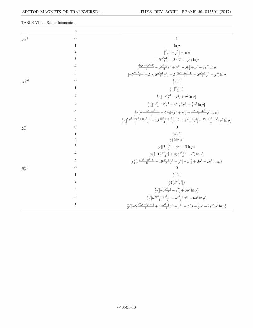
TABLE VIII. Sector harmonics.
n
AðeÞn
0 1
1 ln ρ
2 ½ρ2−12
− y2� − ln ρ
3 ½−3 ρ2−12� þ 3ðρ2þ1
2− y2Þ ln ρ
4 ½3ðρ4þ4ρ2−5Þ8
− 6 ρ2−12
y2 þ y4� − 3ð12þ ρ2 − 2y2Þ ln ρ
5 ½−5 9ðρ4−1Þ16
þ 5 × 6 ρ2−12
y2� þ 5ð3ðρ4þ4ρ2þ1Þ8
− 6 ρ2þ12
y2 þ y4Þ ln ρAðmÞ
n0 1
ρ f1g1 1
ρ f½ρ2−12�g
2 1ρ f½− ρ2−1
2− y2� þ ρ2 ln ρg
3 1ρ f½3ðρ
2þ1Þ4
ρ2−12
− 3 ρ2−12
y2� − 32ρ2 ln ρg
4 1ρ f½− 3ð5ρ4−4ρ2−1Þ
8þ 6 ρ2−1
2y2 þ y4� þ 3ð2þρ2−4y2Þ
2ρ2 ln ρg
5 1ρ f½5ðρ
4þ10ρ2þ1Þ8
ρ2−12
− 103ðρ2þ1Þ
4ρ2−12
y2 þ 5 ρ2−12
y4� − 15ð1þρ2−4y2Þ4
ρ2 ln ρgBðeÞn
0 0
1 yf1g2 yf2 ln ρg3 yf½3 ρ2−1
2− y2� − 3 ln ρg
4 yf½−12 ρ2−12� þ 4ð3 ρ2þ1
2− y2Þ ln ρg
5 yf½5 3ðρ4þ4ρ2−5Þ8
− 10 ρ2−12
y2 þ y4� − 5ð32þ 3ρ2 − 2y2Þ ln ρg
BðmÞn
0 0
1 yρ f1g
2 yρ f½2 ρ2−1
2�g
3 yρ f½−3 ρ2−1
2− y2� þ 3ρ2 ln ρg
4 yρ f½4 3ðρ2þ1Þ
4ρ2−12
− 4 ρ2−12
y2� − 6ρ2 ln ρg5 y
ρ f½−5 3ð5ρ4−4ρ2−1Þ8
þ 10 ρ2−12
y2 þ y4� þ 5ð3þ 32ρ2 − 2y2Þρ2 ln ρg
SECTOR MAGNETS OR TRANSVERSE … PHYS. REV. ACCEL. BEAMS 20, 043501 (2017)
043501-13

APPENDIX E: R- AND S-MULTIPOLES—EXACT EXPRESSIONS
The scalar potentials, longitudinal component of vector potential, and field components for pure R- and S-multipoles upto fifth order are listed in Tables IX and X and Tables XI and XII, respectively.
TABLE X. Horizontal and vertical components of pure normal and skew R-multipole magnets’ field.
n Fx Fy
0 Calibration � � � � � �1 Normal dipole 0 C1
2 Normal quadrupole 11!ðyÞC2
11!ðxÞC2
3 Normal sextupole 12!ð2xyÞC3
12!ðx2 − y2ÞC3
4 Normal octupole 13!ð3x2y − y3ÞC4
13!ðx3 − 3xy2ÞC4
5 Normal decapole 14!ð4x3y − 4xy3ÞC5
14!ðx4 − 6x2y2 þ y4ÞC5
0 Calibration � � � � � �1 Skew dipole C1 0
2 Skew quadrupole 11!ðxÞC2 − 1
1!ðyÞC2
3 Skew sextupole 12!ðx2 − y2ÞC3 − 1
2!ð2xyÞC3
4 Skew octupole 13!ðx3 − 3xy2ÞC4 − 1
3!ð3x2y − y3ÞC4
5 Skew decapole 14!ðx4 − 6x2y2 þ y4ÞC5 − 1
4!ð4x3y − 4xy3ÞC5
TABLE IX. Longitudinal component of the vector potential and scalar potential for pure normal and skew R-multipoles.
n Az Φ
0 Calibration −C0 0
1 Normal dipole − 11!ðxÞC1 − 1
1!ðyÞC1
2 Normal quadrupole − 12!ðx2 − y2ÞC2 − 1
2!ð2xyÞC2
3 Normal sextupole − 13!ðx3 − 3xy2ÞC3 − 1
3!ð3x2y − y3ÞC3
4 Normal octupole − 14!ðx4 − 6x2y2 þ y4ÞC4 − 1
4!ð4x3y − 4xy3ÞC4
5 Normal decapole − 15!ðx5 − 10x3y2 þ 5xy4ÞC5 − 1
5!ð5x4y − 10x2y3 þ y5ÞC5
0 Calibration 0 C0
1 Skew dipole 11!ðyÞC1 − 1
1!ðxÞC1
2 Skew quadrupole 12!ð2xyÞC2 − 1
2!ðx2 − y2ÞC2
3 Skew sextupole 13!ð3x2y − y3ÞC3 − 1
3!ðx3 − 3xy2ÞC3
4 Skew octupole 14!ð4x3y − 4xy3ÞC4 − 1
4!ðx4 − 6x2y2 þ y4ÞC4
5 Skew decapole 15!ð5x4y − 10x2y3 þ y5ÞC5 − 1
5!ðx5 − 10x3y2 þ 5xy4ÞC5
T. ZOLKIN PHYS. REV. ACCEL. BEAMS 20, 043501 (2017)
043501-14

TABLE XI. Azimuthal component of the vector potential and scalar potential for pure normal and skew S-multipoles.
n
AðnÞθ
0 − 10!
1ρ f1gC0
1 − 11!
1ρ f½ρ
2−12�gC1
2 − 12!
1ρ f½− ρ2−1
2− y2� þ ρ2 ln ρgC2
3 − 13!
1ρ f½3ðρ
2þ1Þ4
ρ2−12
− 3 ρ2−12
y2� − 32ρ2 ln ρgC3
4 − 14!
1ρ f½− 3ð5ρ4−4ρ2−1Þ
8þ 6 ρ2−1
2y2 þ y4� þ 3ð2þρ2−4y2Þ
2ρ2 ln ρgC4
5 − 15!
1ρ f½5ðρ
4þ10ρ2þ1Þ8
ρ2−12
− 103ðρ2þ1Þ
4ρ2−12
y2 þ 5 ρ2−12
y4� − 15ð1þρ2−4y2Þ4
ρ2 ln ρgC5
ΦðnÞ 0 0
1 − 11!yf1gC1
2 − 12!yf2 ln ρgC2
3 − 13!yf½3 ρ2−1
2− y2� − 3 ln ρgC3
4 − 14!yf½−12 ρ2−1
2� þ 4ð3 ρ2þ1
2− y2Þ ln ρgC4
5 − 15!yf½5 3ðρ4þ4ρ2−5Þ
8− 10 ρ2−1
2y2 þ y4� − 5ð3
2þ 3ρ2 − 2y2Þ ln ρgC5
AðnÞθ
0 0
1 11!
yρ f1gC1
2 12!
yρ f½2 ρ2−1
2�gC2
3 13!
yρ f½−3 ρ2−1
2− y2� þ 3ρ2 ln ρgC3
4 14!
yρ f½4 3ðρ2þ1Þ
4ρ2−12
− 4 ρ2−12
y2� − 6ρ2 ln ρgC4
5 15!
yρ f½−5 3ð5ρ4−4ρ2−1Þ
8þ 10 ρ2−1
2y2 þ y4� þ 5ð3þ 3
2ρ2 − 2y2Þρ2 ln ρgC5
ΦðnÞ 0 − 10!f1gC0
1 − 11!fln ρgC1
2 − 12!f½ρ2−1
2− y2� − ln ρgC2
3 − 13!f½−3 ρ2−1
2� þ 3ðρ2þ1
2− y2Þ ln ρgC3
4 − 14!f½3ðρ4þ4ρ2−5Þ
8− 6 ρ2−1
2y2 þ y4� − 3ð1
2þ ρ2 − 2y2Þ ln ρgC4
5 − 15!f½−5 9ðρ4−1Þ
16þ 5 × 6 ρ2−1
2y2� þ 5ð3ðρ4þ4ρ2þ1Þ
8− 6 ρ2þ1
2y2 þ y4Þ ln ρgC5
SECTOR MAGNETS OR TRANSVERSE … PHYS. REV. ACCEL. BEAMS 20, 043501 (2017)
043501-15

TABLE XII. Radial and vertical components of pure normal and skew S-multipoles’ field.
n
FðnÞρ
0 Calibration � � �1 Normal dipole 0
2 Normal quadrupole − 11!
yρ f1gC2
3 Normal sextupole − 12!
yρ f½2 ρ2−1
2�gC3
4 Normal octupole − 13!
yρ f½−3 ρ2−1
2− y2� þ 3ρ2 ln ρgC4
5 Normal decapole − 14!
yρ f½4 3ðρ2þ1Þ
4ρ2−12
− 4 ρ2−12
y2� − 6ρ2 ln ρgC5
FðnÞy
0 Calibration � � �1 Normal dipole 1
0!f1gC1
2 Normal quadrupole 11!fln ρgC2
3 Normal sextupole 12!f½ρ2−1
2− y2� − ln ρgC3
4 Normal octupole 13!f½−3 ρ2−1
2� þ 3ðρ2þ1
2− y2Þ ln ρgC4
5 Normal decapole 14!f½3ðρ4þ4ρ2−5Þ
8− 6 ρ2−1
2y2 þ y4� − 3ð1
2þ ρ2 − 2y2Þ ln ρgC5
FðnÞρ
0 Calibration � � �1 Skew dipole 1
0!1ρ f1gC1
2 Skew quadrupole 11!
1ρ f½ρ
2−12�gC2
3 Skew sextupole 12!
1ρ f½− ρ2−1
2− y2� þ ρ2 ln ρgC3
4 Skew octupole 13!
1ρ f½3ðρ
2þ1Þ4
ρ2−12
− 3 ρ2−12
y2� − 32ρ2 ln ρgC4
5 Skew decapole 14!
1ρ f½− 3ð5ρ4−4ρ2−1Þ
8þ 6 ρ2−1
2y2 þ y4� þ 3ð2þρ2−4y2Þ
2ρ2 ln ρgC5
FðnÞy
0 Calibration � � �1 Skew dipole 0
2 Skew quadrupole 11!yf1gC2
3 Skew sextupole 12!yf2 ln ρgC3
4 Skew octupole 13!yf½3 ρ2−1
2− y2� − 3 ln ρgC4
5 Skew decapole 14!yf½−12 ρ2−1
2� þ 4ð3 ρ2þ1
2− y2Þ ln ρgC5
T. ZOLKIN PHYS. REV. ACCEL. BEAMS 20, 043501 (2017)
043501-16

APPENDIX F: TAYLOR POLYNOMIALS OF F n AND Gn
The first ten terms of the Maclaurin series of F nðxÞ, GnðxÞ and GnðxÞ1þx are listed in Table XIII.
TABLE XIII. Maclaurin series of F nðxÞ, GnðxÞ and GnðxÞ1þx ; they are also Taylor polynomials of F nðρÞ, GnðρÞ and GnðρÞ
ρ at ρ ¼ 1.
n TðF nÞ0 1
1 x − 12x2 þ 1
3x3 − 1
4x4 þ 1
5x5 − 1
6x6 þ 1
7x7 − 1
8x8 þ 1
9x9 − 1
10x10 þOðx11Þ
2 x2 − 13x3 þ 1
4x4 − 1
5x5 þ 1
6x6 − 1
7x7 þ 1
8x8 − 1
9x9 þ 1
10x10 − 1
11x11 þOðx12Þ
3 x3 − 12x4 þ 7
20x5 − 11
40x6 þ 8
35x7 − 11
56x8 þ 29
168x9 − 37
240x10 þ 23
165x11 − 7
55x12 þOðx13Þ
4 x4 − 25x5 þ 3
10x6 − 17
70x7 þ 23
112x8 − 5
28x9 þ 19
120x10 − 47
330x11 þ 57
440x12 − 17
143x13 þOðx14Þ
5 x5 − 12x6 þ 5
14x7 − 2
7x8 þ 27
112x9 − 47
224x10 þ 689
3696x11 − 355
2112x12 þ 263
1716x13 − 1129
8008x14 þOðx15Þ
6 x6 − 37x7 þ 9
28x8 − 11
42x9 þ 25
112x10 − 241
1232x11 þ 123
704x12 − 181
1144x13 þ 2319
16016x14 − 535
4004x15 þOðx16Þ
7 x7 − 12x8 þ 13
36x9 − 7
24x10 þ 131
528x11 − 689
3168x12 þ 5339
27456x13 − 9683
54912x14 þ 16
99x15 − 1367
9152x16 þOðx17Þ
8 x8 − 49x9 þ 1
3x10 − 3
11x11 þ 185
792x12 − 353
1716x13 þ 1267
6864x14 − 3457
20592x15 þ 5647
36608x16 − 855
5984x17 þOðx18Þ
9 x9 − 12x10 þ 4
11x11 − 13
44x12 þ 289
1144x13 − 509
2288x14 þ 457
2288x15 − 2
11x16 þ 9461
56576x17 − 192991
1244672x18 þOðx19Þ
n TðGnÞ0 1
1 xþ 12x2
2 x2 þ 13x3 − 1
12x4 þ 1
30x5 − 1
60x6 þ 1
105x7 − 1
168x8 þ 1
252x9 − 1
360x10 þ 1
495x11 þOðx12Þ
3 x3 þ 12x4 − 1
20x5 þ 1
40x6 − 1
70x7 þ 1
112x8 − 1
168x9 þ 1
240x10 − 1
330x11 þ 1
440x12 þOðx13Þ
4 x4 þ 25x5 − 1
10x6 þ 3
70x7 − 13
560x8 þ 1
70x9 − 1
105x10 þ 31
4620x11 − 13
2640x12 þ 8
2145x13 þOðx14Þ
5 x5 þ 12x6 − 1
14x7 þ 1
28x8 − 1
48x9 þ 3
224x10 − 17
1848x11 þ 7
1056x12 − 17
3432x13 þ 61
16016x14 þOðx15Þ
6 x6 þ 37x7 − 3
28x8 þ 1
21x9 − 3
112x10 þ 3
176x11 − 173
14784x12 þ 271
32032x13 − 37
5824x14 þ 59
12012x15 þOðx16Þ
7 x7 þ 12x8 − 1
12x9 þ 1
24x10 − 13
528x11 þ 17
1056x12 − 103
1952x13 þ 151
18304x14 − 43
6864x15 þ 179
36609x16 þOðx17Þ
8 x8 þ 49x9 − 1
9x10 þ 5
99x11 − 23
792x12 þ 97
5148x13 − 271
20592x14 þ 199
20592x15 − 2425
329472x16 þ 1009
175032x17 þOðx18Þ
9 x9 þ 12x10 − 1
11x11 þ 1
22x12 − 31
1144x13 þ 41
2288x14 − 29
2288x15 þ 43
4576x16 − 4489
622336x17 þ 7079
1244672x18 þOðx19Þ
n TðGn=ρÞ0 1 − xþ x2 − x3 þ x4 − x5 þ x6 − x7 þ x8 − x9 þOðx10Þ1 x − 1
2x2 þ 1
2x3 − 1
2x4 þ 1
2x5 − 1
2x6 þ 1
2x7 − 1
2x8 þ 1
2x9 − 1
2x10 þOðx11Þ
2 x2 − 23x3 þ 7
12x4 − 11
20x5 þ 8
15x6 − 11
21x7 þ 29
56x8 − 37
72x9 þ 23
45x10 − 28
55x11 þOðx12Þ
3 x3 − 12x4 þ 9
20x5 − 17
40x6 þ 23
56x7 − 45
112x8 þ 19
48x9 − 47
120x10 þ 171
440x11 − 17
44x12 þOðx13Þ
4 x4 − 35x5 þ 1
2x6 − 16
35x7 þ 243
560x8 − 47
112x9 þ 689
1680x10 − 71
176x11 þ 263
660x12 − 1129
2860x13 þOðx14Þ
5 x5 − 12x6 þ 3
7x7 − 11
28x8 þ 125
336x9 − 241
672x10 þ 123
352x11 − 181
528x12 þ 773
2288x13 − 2675
8008x14 þOðx15Þ
6 x6 − 47x7 þ 13
28x8 − 5
12x9 þ 131
336x10 − 689
1848x11 þ 5339
14784x12 − 9683
27456x13 þ 80
231x14 − 1367
4004x15 þOðx16Þ
7 x7 − 12x8 þ 5
12x9 − 3
8x10 þ 185
528x11 − 353
1056x12 þ 8869
27456x13 − 17285
54912x14 þ 5647
18304x15 − 855
2816x16 þOðx17Þ
8 x8 − 59x9 þ 4
9x10 − 13
33x11 þ 289
792x12 − 3563
10296x13 þ 2285
6864x14 − 32
99x15 þ 9461
29952x16 − 192991
622336x17 þOðx18Þ
9 x9 − 12x10 þ 9
22x11 − 4
11x12 þ 35
104x13 − 729
2288x14 þ 175
572x15 − 1357
4576x16 þ 13851
47872x17 − 353047
1244672x18 þOðx19Þ
SECTOR MAGNETS OR TRANSVERSE … PHYS. REV. ACCEL. BEAMS 20, 043501 (2017)
043501-17

[1] K. L. Brown, SLAC Report No. SLAC-75, 1972, http://cds.cern.ch/record/283218/files/SLAC‑75.pdf.
[2] E. Forest, Beam Dynamics (Harwood Academic Publishers,Amsterdam, 1998), Vol. 8.
[3] H. Wiedemann, Particle Accelerator Physics (Springer,New York, 2015).
[4] E. M. McMillan, Multipoles in cylindrical coordinates,Nucl. Instrum. Methods 127, 471 (1975).
[5] S. Mane, Solutions of Laplace’s equation in two dimensionswith a curved longitudinal axis, Nucl. Instrum. MethodsPhys. Res., Sect. A 321, 365 (1992).
[6] R. A. Beth, Complex representation and computation oftwo‐dimensional magnetic fields, J. Appl. Phys. 37, 2568(1966).
[7] H. Yoshida, Construction of higher order symplectic inte-grators, Phys. Lett. A 150, 262 (1990).
T. ZOLKIN PHYS. REV. ACCEL. BEAMS 20, 043501 (2017)
043501-18