section iv: methods and analysis - alaska

Section IV: Methods and

Analysis

Alaska Geographic Differential Study 2008 McDowell Group, Inc. • Page 51

Introduction

Governments, businesses, and social scientists use estimates of consumer prices and cost of living in a wide

variety of applications, including inequality studies, wage comparisons and poverty assessments. These

estimates address two basic cost parameters: changes over time and differences from place to place. The

federal Consumer Price Index (CPI), the most extensive price-measurement program in the U.S., is an

estimate of inflation. It measures changes in the cost of a specified “market basket” of goods over time in 87

urban areas based on analysis of approximately 80,000 individual prices collected monthly from more than

21,000 retail outlets. One of the best-known geographic differential methodologies is the ACCRA (American

Chamber of Commerce Researchers Association) Cost of Living Index. ACCRA measures differences in cost of

living among roughly 400 urban and suburban areas throughout the U.S.

Because the CPI and geographic-differentials research help determine how billions of dollars in public and

private services, salaries and other investments are allocated, the process of critiquing and refining these

methodologies is ongoing. Alaska, however, remains something of a special case. Whereas many of

methodological adjustments have been designed to address expanding consumer choices, much consumer

behavior in Alaska is driven, instead, by an absence of choices. Things regarded as common necessities in

parts of Alaska, a car for example, either can’t be had or are of limited use in other communities. Such radical

differences in local needs and options affect both the cost and quality of life.

This section of the report discusses some of the methodological considerations that have been addressed in

the past few years in the consumer-price and cost of living literature and how they relate, or fail to relate, to

Alaska.

• McDowell Group, Inc. Alaska Geographic Differential Study 2008

Designing Consumer-Price and Cost of Living Studies

A consumer-price study measures changes in the prices of identical products over time or from place to place.

A cost of living study is more complex. It measures changes in the cost of a defined standard of living over

time or from place to place.1 “Standard of living” means “identical utility” (in the economic sense) or, more

generally, an identical level of well-being. This means that, while consumer price studies are concerned only

with variations in the price of goods and services, cost of living studies include analysis of household

consumption patterns as well as consumer prices. The CPI methodology, while not aspiring to measure true

cost of living, combines methods to track pure price inflation with methods for consumption weighting to

produce a more accurate estimate of the impact of inflation on real families.

Consumer-price and cost of living studies share a number of challenges, including the following:

• For various reasons, different stores in the same community may charge different prices for the same

goods. Both consumer-price and cost of living studies must find ways of determining how much to

weight prices from one store compared to prices from another.

• Changes in product design, technology and availability mean that the set of goods and services to be

compared is not identical over time and often varies from place to place as well. In Alaska, for

example, sales of new outboard motors have evolved over the past few years from predominantly

two-stroke engines to predominantly four-stroke engines (with associated changes in price and

performance).

Regional cost of living studies must confront special challenges, including the following:

• Consumer spending is affected not just by market prices and consumer preferences, but by non-

market goods such as public infrastructure, climatic conditions, the crime rate, etc. For example, the

outboard engines described above are virtual necessities in many parts of the state and virtually

irrelevant in others. This variability affects both price and demand.

• Some sectors of consumer spending vary significantly from place to place, or are so complex that it

becomes difficult to identify comparable products and prices. One example is medical care, where

prices vary depending on what types of services and third-party payers are available.

In Alaska, differences in climate, transportation, service availability, and other factors can be so extreme as to

make it virtually impossible to define key components of a standard of living in diverse communities. An

example is housing. In most communities in rural Alaska, building and maintaining a house that is average for

Anchorage would be prohibitively expensive for all but the wealthiest families. The Alaska GDS approach

developed to address this and other challenges is described later in this section.

1 Hoffmeister, Onno. “Cost of Living and Real Income Differentials in Russia’s Provinces: Evidence from the Russia Longitudinal Monitoring Survey,” Institute for Eastern European Studies, Berlin, 2003.

Alaska Geographic Differential Study 2008 McDowell Group, Inc. • 3

Developing Cost of Living Indexes

Like many economic measures, cost-of-living indexes must be interpreted within a set of assumptions that

limits their application. If all consumers had the same preferences and income, price differentials would be

wholly sufficient. Since preferences and income are affected by demographics, location, ethnicity,

technology, access to information, and many other factors, even the most sophisticated cost of living

methodologies, such as the CPI, fall short of pinpoint accuracy. Following is a brief discussion of how the field

has tried to address three fundamental components of cost of living studies:

• Consumption weights

• Sampling

• Market basket

Consumption Weights

Price differentials, alone, can be a useful indicator of the cost of living. It is more accurate, however, to

“weight” prices using information about consumption: what people actually buy. Consumption is affected by

price, but also by need and preference. All three factors (price, need, and preference) vary from place to place

and over time. Determining which goods, services, and prices are most relevant and important –– and

therefore deserve the most weight –– is a key part of cost-of-living methodologies.

Two of the most common indexes for comparing cost of living are known as the Laspeyres Index and the

Paasche Index. The two methods differ principally in what set of circumstances is used for the base

calculation and what is used as the comparison. Each method leads to a slightly different mathematical result.

A third method computes a geometric mean of the Laspeyres and Paasche Indexes. This is also known as the

Fisher Ideal index.2

In practice, most cost of living studies use the Laspeyres Index because it relies on consumption patterns from

the base region or base time period. Typically, base consumption patterns are known or represent the least

cost to obtain. The Paasche Index requires consumption patterns from each new comparison region or time

period, and the Fisher Index requires both. This means that, the Paasche and Fisher indexes require new

consumption data for each new computation, while the Laspeyres Index may be computed for multiple time

periods or locations using a single set of (base) consumption data.

Sampling

The ideal data for establishing geographic cost of living differentials would be a record of all household

purchases (including all prices and all quantities) for all households in all regions of interest. It is clearly

impractical to obtain data for all households, nor is it practical to obtain all prices and quantities. Cost of

living indexes address these data shortcomings by sampling in a variety of ways, and an extensive body of

literature has developed that evaluates the pros and cons of different methods.3 All the sampling methods

must address three basic parameters for both the base region and comparison region:

2 Ibid. pages 23-24. 3 Many of the basic issues involved in constructing and updating price indexes are summarized in the book, At What Price, by the National Research Council’s Panel on Conceptual, Measurement, and Other Statistical Issues in Developing Cost-of-Living Indexes (2002, National Academy Press).


1. How does a representative household distribute its expenditures across all possible purchases?

2. What subset of items provides the best proxy for the range of actual items purchased?

3. What subset of local prices provides the best proxy for the range actual prices paid?

Typical methodologies include data collection from a sample of households (regarding purchases) and a

sample of retail outlets (regarding prices and sales). In all cases, sampling plans must address the weighting

considerations described above.

Market Basket

The concept of pricing comparable market baskets to measure price differences from time to time or place to

place is deceptively simple. In practice, it is impossible to price a broad enough set of precisely the same

items to obtain a wholly accurate comparison of overall living costs. Following is a brief discussion of some of

the more material adjustments that may need to be considered in market basket methodologies.

SUBSTITUTION

Substitution refers to the fact that, over time or from place to place, consumers may purchase certain goods

and services in lieu of others. For example, Delicious apples may substitute for Gala apples depending on

season or location. This means that it is seldom possible to recreate in the comparison time period or region

precisely the same market basket as was priced in the base. As a result, the BLS began using geometric

instead of arithmetic averaging to combine individual prices in approximately 60 percent of the market

basket strata used in the CPI.4

Substitution occurs over time, but is even more of a challenge from place to place. There are more

substitution possibilities in urban areas than in rural areas.5 Also, Curran et al (2006) argued that the set of

choices available to different consumers is not the same. For example, wealthier households can afford to

exercise greater choice not just because they can spend more, but because they are more mobile. Low-

income households cannot respond as quickly to geographic price differences because they tend to have less

money to cover moving costs, less information about work opportunities, less human capital (for example,

less developed networks), and generally less capacity to explore options.

QUALITY

The effect of quality differences in similar goods and services is related to that of substitution. When two

items are similar but one is of higher quality, the price premium for that quality reflects delivery of greater

benefits to the consumer. If the benefits realized by the consumer are different, then the increase in price

cannot, at least entirely, be attributed to inflation or an increased cost of living. Quality of life also increases as

a result of the new benefits. For example, differences in the cost of cable television service may reflect

increases in the amount of and quality of programming, high-definition picture, pay-per-view options, etc.

4 Schultze and Mackie, Editors, At What Price, Panel on Conceptual, Measurement, and Other Statistical Issues in Developing Cost-of-Living Indexes, National Academy Press, 2002. 5 Ravallion, Martin and Dominique van de Walle, “Urban-Rural Cost-of-Living Differentials in a Developing Economy,” Journal of Urban Economics 29, 113-127, 1991.


CHOICE OF RETAIL OUTLET

Cost-of-living methodologies must try to estimate the effects on pricing of the types of retail outlets where

people actually shop. To the extent possible, sample prices should be weighted to reflect the proportion of

consumers who shop at, for example, box stores (lower prices) versus full-service specialty stores (higher

prices). Ideally, a COLI methodology should also account for the decline in “utility” (increase in cost of living)

for consumers who prefer to shop in a full-service outlet, but who have found those stores driven out of

business by the new outlets. However, the BLS has found the latter type of adjustment to be impractical and

of minor impact.6

AGGREGATING DATA FROM INDIVIDUAL HOUSEHOLDS

Every household faces a unique cost of living (and, arguably, a unique rate of inflation). That is, no two

households make precisely the same set of purchases, and, in theory, one could create an individual cost of

living index for each household.7 To produce an aggregated index requires averaging across households, and

this may be done either with a simple average (equal weight to each household) or a weighted average (with

households that spend more given more weight. The former is known as a “democratic” index, the latter as

“plutocratic.”

The practical limitation to either democratic or plutocratic aggregation across all households is simply the task

of collecting individual data from all households. Schultze and Mackie suggest that the BLS consider an

intermediate approach for the CPI, namely aggregating sub-indexes for defined groups, such as the poor and

the elderly. They also point out, however, that there is not yet conclusive evidence such groups experience

significantly different inflation rates over extended time periods.

HOUSING

Housing is a heterogeneous good. That means there is no single measure that represents the quantity

consumed. Instead, observed market prices more accurately represent expenditures on a bundle of diverse

housing attributes such as age of structure, climate, location (for example, roaded vs. non-roaded, distance to

markets, or distance to green space), quality (of windows, toilet, kitchen, water, laundry, etc.), size, cultural

attributes (traditional vs. modern building methods), etc. Housing is also a matter of consumer choice and

income. Ravallion and van de Walle use a hedonic rent model to deal with some of the problems posed by

heterogeneity.8 In practice, however, a hedonic housing-cost-index would be time-intensive, difficult to

calculate, and expensive.

Unlike other consumer goods, housing is not traded spatially (cannot be moved from place to place), which

can greatly amplify price differentials.

MEDICAL CARE

Schultze and Mackie describe the issues associated with developing the medical care component of the CPI

as more difficult than those of any other component. Technological progress and institutional evolution result

in changing quality of care. Further complexity is introduced by the fact that many factors besides type and

6 Schultze and Mackie, op. cit. page 251. 7 “The Boskin Commission Report: Toward a More Accurate Measure of the Cost of Living,” Report to the Senate Finance Committee, 1996:5. 8 Hedonic pricing varies according to the qualities or attributes associated with individual purchases.


quality of care determine an individual’s health. This leads to the question whether cost-of-living measures

should be associated with inputs (a prescription, a physician visit, or a day in the hospital) or outputs, namely

changes in health. Other questions abound, for example how an index should treat a relatively inexpensive

condition that many people face, such as conjunctivitis, versus a more rare, but much more expensive

condition such as heart disease. Finally, the issues are compounded by the different ways in which consumers

pay for medical care, including variations in insurance coverage and cost and who pays the premiums. Even

for a study of the scale of the CPI, substantial uncertainty exists about the precision of current methods.

However, recommendations in Schultze and Mackie for potential improvements would require extensive

analysis of medical outcomes under multiple treatment scenarios.9

Differentials Research in Alaska

As noted above, computing regional cost of living differentials requires generalizing about a variety of

communities using sample data from households and retail outlets. The Alaska GDS methodology includes

many design elements to address the special challenges of conducting this research in Alaska to the extent

practical. However, extraordinary time and resources would be needed to overcome all of them completely,

for example:

• The challenge of obtaining price data on site in far-flung, isolated communities.

• The challenge of supplementing telephone survey data about household expenditures with more

detailed information from, for example, expenditure diaries, and lengthy personal interviews. Both of

these supplementary methods are employed in CPI research.

• The fact that many items considered essential in some communities are either not available or not

needed in other communities, due to differences in geography and lifestyle.

• The large impact that transportation, shipping, climate, and other factors can have on prices and

consumption in specific areas of the state. For example, recent research by the Institute for Social and

Economic Research (ISER) demonstrated that shipping anomalies, storage capacity, and other factors

can result in large differences in fuel costs between communities that are located relatively close to

one another.

9 Schultze and Mackie, op. cit. pages 188 – 190.


Alaska GDS 2008 Methodology

Introduction

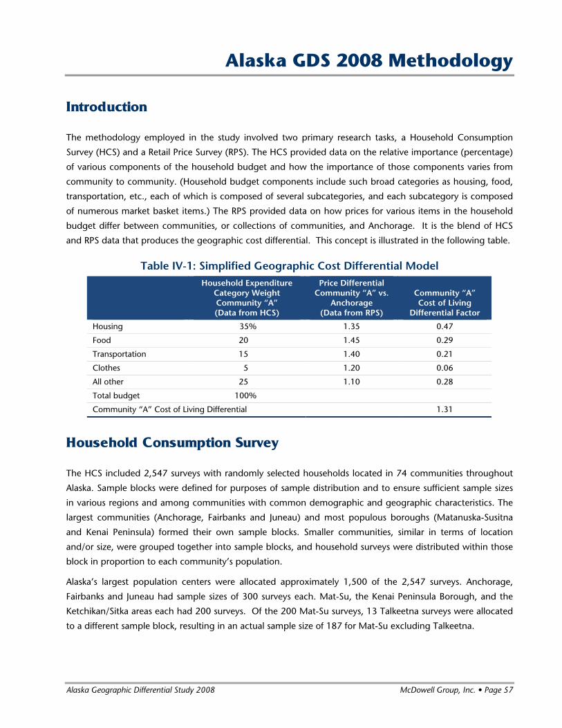
The methodology employed in the study involved two primary research tasks, a Household Consumption

Survey (HCS) and a Retail Price Survey (RPS). The HCS provided data on the relative importance (percentage)

of various components of the household budget and how the importance of those components varies from

community to community. (Household budget components include such broad categories as housing, food,

transportation, etc., each of which is composed of several subcategories, and each subcategory is composed

of numerous market basket items.) The RPS provided data on how prices for various items in the household

budget differ between communities, or collections of communities, and Anchorage. It is the blend of HCS

and RPS data that produces the geographic cost differential. This concept is illustrated in the following table.

Table IV-1: Simplified Geographic Cost Differential Model

Household Expenditure Category Weight Community “A” (Data from HCS)

Price Differential Community “A” vs.

Anchorage (Data from RPS)

Community “A” Cost of Living

Differential Factor

Housing 35% 1.35 0.47

Food 20 1.45 0.29

Transportation 15 1.40 0.21

Clothes 5 1.20 0.06

All other 25 1.10 0.28

Total budget 100%

Community “A” Cost of Living Differential 1.31

Household Consumption Survey

The HCS included 2,547 surveys with randomly selected households located in 74 communities throughout

Alaska. Sample blocks were defined for purposes of sample distribution and to ensure sufficient sample sizes

in various regions and among communities with common demographic and geographic characteristics. The

largest communities (Anchorage, Fairbanks and Juneau) and most populous boroughs (Matanuska-Susitna

and Kenai Peninsula) formed their own sample blocks. Smaller communities, similar in terms of location

and/or size, were grouped together into sample blocks, and household surveys were distributed within those

block in proportion to each community’s population.

Alaska’s largest population centers were allocated approximately 1,500 of the 2,547 surveys. Anchorage,

Fairbanks and Juneau had sample sizes of 300 surveys each. Mat-Su, the Kenai Peninsula Borough, and the

Ketchikan/Sitka areas each had 200 surveys. Of the 200 Mat-Su surveys, 13 Talkeetna surveys were allocated

to a different sample block, resulting in an actual sample size of 187 for Mat-Su excluding Talkeetna.


Table IV-2: Household Consumption Survey Sample Sizes Sample Block Sample Size

1: Anchorage 300

2: Fairbanks 300

3: Parks/Elliott/Steese Highways 65

4: Glennallen Region 50

5: Delta Junction/Tok Region 76

6: Roadless Interior 51

7: Juneau 300

8: Ketchikan/Sitka 200

9: Southeast Mid-Size Communities 104

10: Southeast Small Communities 52

11: Mat-Su 187

12: Kenai Peninsula 200

13: Prince William Sound 100

14: Kodiak 104

15: Arctic Region 153

16: Bethel/Dillingham 151

17: Aleutian Region 77

18: Southwest Small Communities 77

The 50-question HCS collected data on household spending related to housing (including mortgage and rent

payment, property taxes, insurance and all utilities), food, transportation, health care, and clothing. The

survey also collected data on household size and income. The survey was fielded during October and

November 2008.

HCS data management was handled in the statistical software package SPSS. An extensive data cleaning

process removed outlier or other irregular values from the analysis. The data management process and SPSS

syntax are described in detail in the Statistical Analysis section of this report.

Perhaps the most important data management tool employed was weighting the HCS data so that it

represented the demographics of communities more accurately than through a strictly random sample

telephone survey data collection effort. For example, telephone survey research is likely to produce

disproportionate representation of older, higher income, home-owning households. Younger households are

typically more active and therefore less likely to be at home when a surveyor calls. As another example of

potential age bias, approximately 12 to 13 percent of Alaska households have only cell phone service, with no

conventional land-line phone service. These households (typically urban) would not be captured in a random

sample survey (because lists of cell phone numbers are not available for purposes of survey research). These

cell-phone-only households are likely to be younger, less likely to own a home, and probably somewhat

lower-income than their older neighbors.

To adjust for these potential biases in the survey data, community-level data was weighted using 2000 census

information on the proportion of homeowners versus renters. For example, 77 percent of the Anchorage

household survey sample were homeowners, while 23 percent were renters. However, the 2000 census

found that 60 percent of the occupied housing units in Anchorage are owner-occupied and 40 percent


renter-occupied. (More recently, the 2006 American Community Survey found a 61 percent home ownership

rate in Anchorage.) Therefore Anchorage survey data was weighted so that household spending patterns of

owners and renters were accurately reflected in the analysis.

Retail Price Survey

The Retail Price Survey (RPS) included 634 retail outlets in 58 communities throughout Alaska, plus numerous

providers of various services, including health care, transportation, communications, insurance, and others. A

market basket of approximately 200 goods and services was priced in each community where they were

available. Data was collected in person and by telephone in the communities listed in the following table.

Table IV-3: Communities included in Retail Price Survey (RPS) Community In Person Phone/Fax Community In Person Phone/Fax

Anchor Point X Kotzebue X

Anchorage X Manley Hot Springs X

Aniak X McGrath X

Barrow X Metlakatla X

Bethel X Nenana X

Cantwell X Ninilchik X

Central X Nome X

Chitina X Palmer X

Cordova X Pelican X

Craig X Petersburg X

Delta Junction X Saint Mary's X

Dillingham X Sand Point X

Eagle X Seldovia X

Emmonak X Seward X

Fairbanks/North Pole X Sitka X

Fort Yukon X Skagway X

Galena X Soldotna X

Glennallen X Talkeetna X

Gustavus X Teller X

Haines X Tenakee Springs X

Healy X Tok X

Homer X Unalakleet X

Hoonah X Unalaska/Dutch Harbor X

Juneau X Valdez X

Kenai X Wasilla X

Ketchikan X Whittier X

King Cove X Willow X

Klawock X Wrangell X

Kodiak X Yakutat X

Multiple retail outlets were surveyed for each category of retail items. Using groceries as an example, eight

stores were surveyed in Anchorage, six in Juneau and six in Fairbanks. In other communities, depending on


the size of the community (and number of local retail outlets), as many as four grocery outlets were surveyed,

though in the smallest communities, the survey was necessarily limited to one or two local stores.

All RPS pricing data was compiled and managed in Excel. This data also underwent an extensive cleaning

process in which outlier values were removed prior to calculating average prices among specific items.

Average prices for a particular item in each community were compared to the average price for the same

item in Anchorage to produce a price differential. These individual item price differentials were then

averaged with price differentials for other items in the same subcategory of items. For example, the price

differential for hot dogs was averaged with the price differential for boneless chicken breasts and several other

meat products to determine a subcategory “meats, poultry and fish” average-price differential.

When communities were grouped together to produce sample block or district differentials, all pricing data

was weighted according to community population. Where applicable, sales taxes were applied to all retail

items. Detailed information regarding the RPS methodology is provided in the Data Collection Methodology

section.


Methods and Analysis by Budget Component

Housing

Calculation of housing cost differentials differs from other components of the household budget in that all

supporting data was derived from the HCS. Extensive data related to housing costs was collected, including

electric power costs, home heating oil costs, etc., but this information was used only as a tool to cross-

reference the results of the HCS, which collected detailed housing cost data. In the HCS, households were

asked:

• If they own or rent their home.

• The amount of their monthly mortgage or rental payment.

• If their mortgage payment includes property taxes and insurance, and if not, the amount of those

annual payments.

• The size of their home, in terms of square feet and number of bedrooms.

• Total monthly or annual payments for electricity, heating oil, natural gas, propane, water, sewer, and

garbage disposal.

With this information, sample block and community-level averages were calculated for monthly shelter costs,

including mortgage (with property taxes and insurance, when applicable) and rent, and total monthly utilities

costs. Community and sample block averages are weighted according to the percentage of owners and

renters.

Average monthly shelter costs, monthly heat/utilities costs, and total monthly housing costs are provided in

the following table for each sample block and for selected individual communities. Table IV-4 also provides

the average total cost per square foot of living space for each sample block and community.

HCS sample sizes are also provided for each sample block and community. Readers should refer to the HCS

methodology discussion in Section V for information on the margin of error associated with various sample

sizes.


Table IV-4: Average Total Monthly Housing Costs and Average Monthly Cost Per Square Foot

Sample Block/Community HCS Sample

Size Shelter Cost Heat/

Utilities Cost Total

Housing Cost

Sample Blocks 1 Anchorage 300 $1,303 $242 $1,545 2 Fairbanks 300 1,097 422 1,519 3 Parks/Elliott/Steese Highways 65 578 415 993 4 Glennallen Region 50 590 546 1,136 5 Delta Junction/Tok Region 76 712 434 1,146 6 Roadless Interior 51 352 545 897 7 Juneau 300 1,263 386 1,649 8 Ketchikan/Sitka 200 1,033 389 1,422 9 Southeast Mid-Size

Communities 105 689 443 1,132

10 Southeast Small Communities 51 579 433 1,012 11 Mat-Su 187 1,047 279 1,326 12 Kenai Peninsula 200 719 301 1,020 13 Prince William Sound 100 892 528 1,421 14 Kodiak 104 1,019 478 1,497 15 Arctic Region 153 942 452 1,394 16 Bethel/Dillingham 151 995 661 1,656 17 Aleutian Region 77 1,006 639 1,645 18 Southwest Small Communities 77 402 606 1,008 Communities

Barrow 66 $1,022 $295 $1,317 Bethel 106 1,073 667 1,740 Cordova 37 733 497 1,230 Dillingham 45 805 646 1,450 Homer 26 799 449 1,248 Ketchikan 107 1,044 391 1,435 Kotzebue 44 815 536 1,351 Nome 48 1,049 550 1,599 Petersburg 30 815 354 1,169 Sitka 80 1,015 387 1,402 Unalaska/Dutch Harbor 51 1,235 597 1,832 Valdez 60 995 555 1,549

Total monthly housing costs were used to calculate the percentage of the total household budget that is

spent on housing. To calculate the contribution of housing costs to the overall sample block/community

geographic cost differential, housing’s share of the total household budget was multiplied by the housing

cost differential.

The housing cost differential was calculated as:

(Sample block or community monthly housing costs per square foot) / (Anchorage monthly housing costs per square foot) = Sample block or community housing cost differential


For example, the average per-square-foot cost of housing in Anchorage was measured at $1.09. The average

cost in Juneau was $1.24. Dividing the Juneau average cost by the Anchorage average cost produced a cost

differential of 1.14. The calculations are the same for an area with lower housing costs than Anchorage. For

example, the average cost of housing in the Mat-Su Borough was measured at $0.86 per square foot.

Dividing that figure by the Anchorage average cost produced a cost differential of 0.79.

Table IV-5: Average Monthly Housing Costs Per Square Foot and Housing Cost Differential

Sample Block/Community

Ave. Housing

Square Foot

Average Cost per

Square Foot Housing Cost Differential

Sample Blocks 1 Anchorage 1,651 $1.09 1.00 2 Fairbanks 1,597 1.06 0.98 3 Parks/Elliott/Steese Highways 1,444 0.81 0.74 4 Glennallen Region 1,511 0.79 0.72 5 Delta Junction/Tok Region 1,614 0.99 0.91 6 Roadless Interior 1,102 0.88 0.81 7 Juneau 1,493 1.24 1.14 8 Ketchikan/Sitka 1,581 1.10 1.01 9 Southeast Mid-Size Communities 1,609 0.80 0.74 10 Southeast Small Communities 1,558 0.73 0.67 11 Mat-Su 1,726 0.86 0.79 12 Kenai Peninsula 1,561 0.85 0.78 13 Prince William Sound 1,725 0.98 0.90 14 Kodiak 1,594 1.12 1.03 15 Arctic Region 1,208 1.32 1.22 16 Bethel/Dillingham 1,276 1.68 1.54 17 Aleutian Region 1,296 1.54 1.42 18 Southwest Small Communities 1,327 0.82 0.75 Communities

Barrow 1,360 $1.17 1.08 Bethel 1,242 1.88 1.73 Cordova 1,741 0.87 0.80 Dillingham 1,357 1.16 1.06 Homer 1,673 0.86 0.79 Ketchikan 1,639 0.97 0.89 Kotzebue 1,053 1.55 1.42 Nome 1,200 1.34 1.24 Petersburg 1,673 0.80 0.74 Sitka 1,496 1.27 1.17 Unalaska/Dutch Harbor 1,182 1.80 1.65 Valdez 1,738 1.06 0.97

Note: The average cost-per-square foot data presented in this table cannot be generated from other data provided in this and the preceding tables. In the housing cost differential model, all of the various calculations are performed separately for homeowners and renters until a weighted average cost per square foot is calculated.


A range of housing-related data was collected to support the analysis of housing cost differentials, including

electric power rates, home heating fuel prices, and natural gas prices. This information is included in the

appendices.

Food

Calculation of the food portion of geographic cost differentials involved collecting data on weekly or monthly

household food expenditures in seven subcategories and retail price data for a market basket of 80 individual

food items. These two sets of data were modeled to produce cost differentials in six food subcategories:

• Meats, poultry, and fish

• Cereals and breads

• Dairy products

• Fruits and vegetables

• Other food items

• Food away from home.

The HCS queried households on their weekly spending in the following food categories:

• Meats, poultry, and fish

• Cereals and breads

• Dairy products

• Fruits and vegetables

• Soups, frozen meals, and snacks

• Nonalcoholic beverages other than milk.

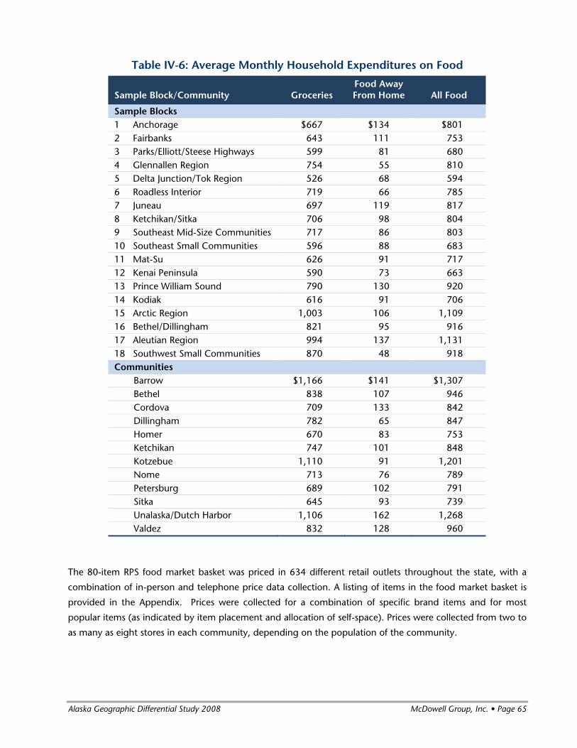
The HCS also collected data on households’ monthly spending at restaurants and on take-out food. HCS

data was not collected on household expenditures on alcohol or tobacco. The following table provides total

monthly spending on food for each sample block and selected communities. Total monthly food costs range

from a low of approximately $600 to a high of approximately $1,300. These costs reflect the price of food in

each sample block or community, as well as average household incomes (higher-income households are likely

to spend more on food than lower income households, all other factors being equal).

See table next page


Table IV-6: Average Monthly Household Expenditures on Food

Sample Block/Community Groceries Food Away From Home All Food

Sample Blocks 1 Anchorage $667 $134 $801 2 Fairbanks 643 111 753 3 Parks/Elliott/Steese Highways 599 81 680 4 Glennallen Region 754 55 810 5 Delta Junction/Tok Region 526 68 594 6 Roadless Interior 719 66 785 7 Juneau 697 119 817 8 Ketchikan/Sitka 706 98 804 9 Southeast Mid-Size Communities 717 86 803 10 Southeast Small Communities 596 88 683 11 Mat-Su 626 91 717 12 Kenai Peninsula 590 73 663 13 Prince William Sound 790 130 920 14 Kodiak 616 91 706 15 Arctic Region 1,003 106 1,109 16 Bethel/Dillingham 821 95 916 17 Aleutian Region 994 137 1,131 18 Southwest Small Communities 870 48 918 Communities

Barrow $1,166 $141 $1,307 Bethel 838 107 946 Cordova 709 133 842 Dillingham 782 65 847 Homer 670 83 753 Ketchikan 747 101 848 Kotzebue 1,110 91 1,201 Nome 713 76 789 Petersburg 689 102 791 Sitka 645 93 739 Unalaska/Dutch Harbor 1,106 162 1,268 Valdez 832 128 960

The 80-item RPS food market basket was priced in 634 different retail outlets throughout the state, with a

combination of in-person and telephone price data collection. A listing of items in the food market basket is

provided in the Appendix. Prices were collected for a combination of specific brand items and for most

popular items (as indicated by item placement and allocation of self-space). Prices were collected from two to

as many as eight stores in each community, depending on the population of the community.


The following steps were taken to develop geographic price differentials for each of the six food

subcategories:

• Collect price data from multiple stores for each of the 80 items in the market basket.

• Clean data to ensure comparability of prices for specific items. In some instances, price data for

specific items was excluded from the analysis if the price was an obvious outlier (the price was far

below or far above prices for the same item in other stores in that community). Sale prices were not

included in the sample.

• Calculate a weighted average price for each item, with prices weighted according to the results of

question 25 in the HCS, which asked respondents where they did a majority of their grocery

shopping. This step was necessary to ensure that the price of an item at a small convenience store

did not have the same affect on average pricing as does the price of the same item from a store

where many more people shop and the item is sold in much greater quantities.

• Apply sales tax in locations where such taxes are levied. This increased the price of each item by the

sales tax rate and produced the actual price paid by the consumer.

• Calculate price differentials for each item by dividing each item’s weighted average price by the

weighted average price of the same item in Anchorage.

• Calculate the average price differential for all items in each subcategory.

• Minimize the potential for an unrepresentative price or set of prices for a particular item to skew the

overall differential for a food subcategory. This was accomplished by removing the highest and

lowest average prices for specific food items from the calculation of the average price differential for

each subcategory. In a majority of cases (but not all), the average differential without the high and

low weighted average prices was nearly identical to the average differential including all items in the

subcategory.

Summary data for food cost geographic differentials are presented in the following table. The table presents

the total expenditure weight for the food portion of the household budget (ranging between 14 percent and

20 percent) and the overall average price differential for all food items (ranging from 1.00 to 1.84).

See table next page


Table IV-7: Food Cost Expenditure Weights and Price Differentials

Sample Block/Community Expenditure

Weights Price

Differential

Sample Blocks 1 Anchorage 0.17 1.00 2 Fairbanks 0.16 1.03 3 Parks/Elliott/Steese Highways 0.16 1.10 4 Glennallen Region 0.20 1.09 5 Delta Junction/Tok Region 0.14 1.09 6 Roadless Interior 0.17 1.55 7 Juneau 0.15 1.03 8 Ketchikan/Sitka 0.17 1.17 9 Southeast Mid-Size Communities 0.18 1.22 10 Southeast Small Communities 0.18 1.22 11 Mat-Su 0.16 1.03 12 Kenai Peninsula 0.19 1.15 13 Prince William Sound 0.17 1.31 14 Kodiak 0.17 1.33 15 Arctic Region 0.18 1.69 16 Bethel/Dillingham 0.15 1.70 17 Aleutian Region 0.18 1.46 18 Southwest Small Communities 0.19 1.79 Communities

Barrow 0.18 1.78 Bethel 0.15 1.72 Cordova 0.15 1.42 Dillingham 0.16 1.64 Homer 0.18 1.13 Ketchikan 0.17 1.18 Kotzebue 0.19 1.84 Nome 0.17 1.51 Petersburg 0.14 1.25 Sitka 0.17 1.15 Unalaska/Dutch Harbor 0.17 1.43 Valdez 0.18 1.26


Transportation

The transportation category includes seven subcategories:

• Fuel for all vehicles

• Car/truck ownership

• All other vehicle ownership

• Auto insurance

• Vehicle maintenance

• Interstate air travel

• Instate air/ferry travel

In the HCS, households were asked for:

• Monthly spending on fuel for all vehicles

• Monthly payments for vehicles of all types (by type of vehicle)

• Total spending in the last 12 months on maintenance for all vehicles

• Total spending in the last 12 months on insurance for all vehicles

• Total spending in the last 12 months on plane tickets for destinations outside of Alaska, not including

business travel

• Total spending in the last 12 months on plane tickets for destinations within Alaska, not including

business travel. (Average total annual household spending on ferry travel was compiled directly from

AMHS data.)

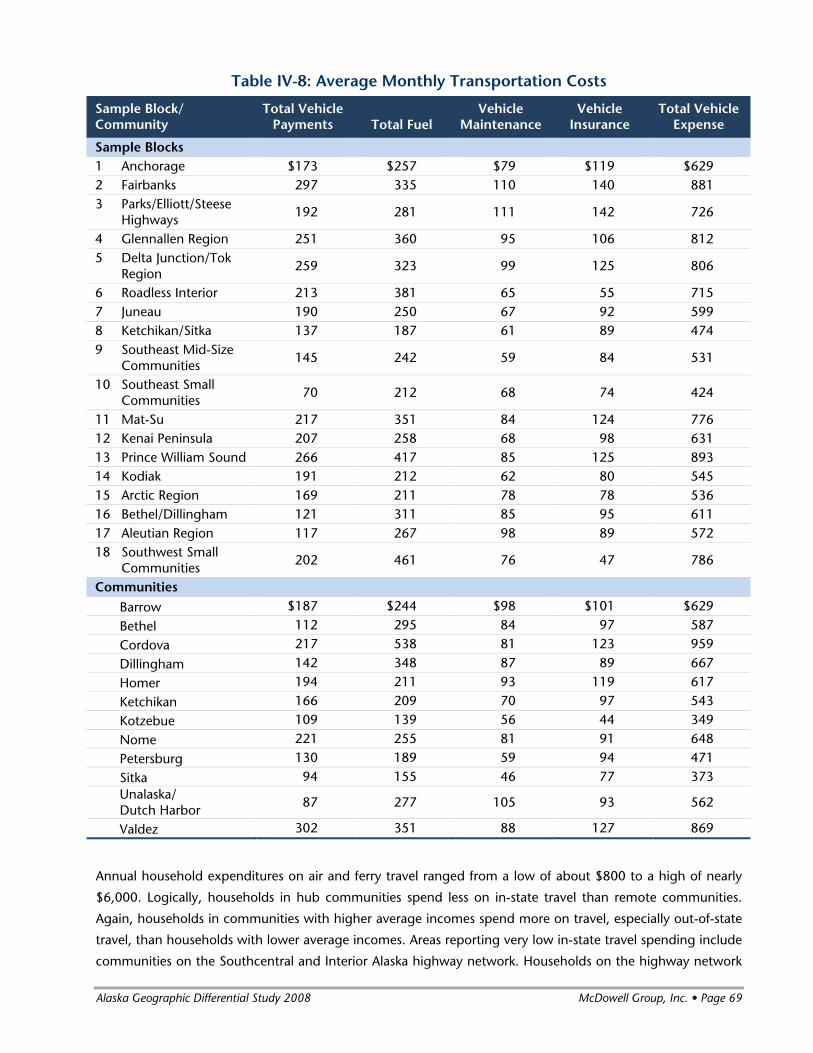
Total vehicle expense (including vehicle payments on loans, fuel, maintenance, and insurance) ranged from a

low of $424 a month to a high of $959. A variety of factors influence vehicle-related spending, including the

extent of road infrastructure in and around each community, cost of fuel, geographic setting (with boats

more prevalent in some areas, and snowmachines and four-wheelers more prevalent in others), average

household income (with higher income households likely to own more vehicles), and other factors. It is

important to note that record high fuel prices in 2008 are reflected in this data and that differences in costs

between urban and rural areas are likely exaggerated relative to previous years (or future years) when prices

are more moderate.

See table next page


Table IV-8: Average Monthly Transportation Costs

Sample Block/ Community

Total Vehicle Payments Total Fuel

Vehicle Maintenance

Vehicle Insurance

Total Vehicle Expense

Sample Blocks 1 Anchorage $173 $257 $79 $119 $629 2 Fairbanks 297 335 110 140 881 3 Parks/Elliott/Steese

Highways 192 281 111 142 726

4 Glennallen Region 251 360 95 106 812 5 Delta Junction/Tok

Region 259 323 99 125 806

6 Roadless Interior 213 381 65 55 715 7 Juneau 190 250 67 92 599 8 Ketchikan/Sitka 137 187 61 89 474 9 Southeast Mid-Size

Communities 145 242 59 84 531

10 Southeast Small Communities 70 212 68 74 424

11 Mat-Su 217 351 84 124 776 12 Kenai Peninsula 207 258 68 98 631 13 Prince William Sound 266 417 85 125 893 14 Kodiak 191 212 62 80 545 15 Arctic Region 169 211 78 78 536 16 Bethel/Dillingham 121 311 85 95 611 17 Aleutian Region 117 267 98 89 572 18 Southwest Small

Communities 202 461 76 47 786

Communities Barrow $187 $244 $98 $101 $629 Bethel 112 295 84 97 587 Cordova 217 538 81 123 959 Dillingham 142 348 87 89 667 Homer 194 211 93 119 617 Ketchikan 166 209 70 97 543 Kotzebue 109 139 56 44 349 Nome 221 255 81 91 648 Petersburg 130 189 59 94 471 Sitka 94 155 46 77 373 Unalaska/ Dutch Harbor 87 277 105 93 562

Valdez 302 351 88 127 869

Annual household expenditures on air and ferry travel ranged from a low of about $800 to a high of nearly

$6,000. Logically, households in hub communities spend less on in-state travel than remote communities.

Again, households in communities with higher average incomes spend more on travel, especially out-of-state

travel, than households with lower average incomes. Areas reporting very low in-state travel spending include

communities on the Southcentral and Interior Alaska highway network. Households on the highway network


probably travel to hub communities more often than households off the highway network, but their travel

costs are captured in the vehicle expense data presented above.

Table IV-9: Average Annual Household Expenditures on Air/Ferry Travel


In-State Air/Ferry

Travel Out-of-State

Air Travel Total Travel Sample Blocks 1 Anchorage $156 $1,639 $1,794 2 Fairbanks 255 1,831 2,086 3 Parks/Elliott/Steese Highways 395 1,694 2,089 4 Glennallen Region 12 815 827 5 Delta Junction/Tok Region 276 697 973 6 Roadless Interior 2,903 887 3,790 7 Juneau 430 1,760 2,190 8 Ketchikan/Sitka 367 1,536 1,903 9 Southeast Mid-Size Communities 509 1,055 1,565 10 Southeast Small Communities 1,009 1,056 2,065 11 Mat-Su 92 926 1,018 12 Kenai Peninsula 384 982 1,366 13 Prince William Sound 680 2,006 2,686 14 Kodiak 596 1,578 2,173 15 Arctic Region 2,233 2,170 4,403 16 Bethel/Dillingham 1,941 1,342 3,283 17 Aleutian Region 2,398 1,984 4,382 18 Southwest Small Communities 2,142 1,319 3,461 Communities

Barrow $3,219 $2,759 $5,978 Bethel 2,160 1,501 3,660 Cordova 755 2,255 3,010 Dillingham 1,432 974 2,407 Homer 327 877 1,204 Ketchikan 224 1,463 1,686 Kotzebue 2,469 2,823 5,292 Nome 1,099 1,145 2,244 Petersburg 475 1,506 1,981 Sitka 583 1,647 2,229 Unalaska/Dutch Harbor 2,711 2,391 5,103 Valdez 649 1,893 2,542

The RPS produced the following transportation-related price data, which was used to calculate cost

differentials in each of the six transportation sub-categories:

• Regular unleaded gasoline and diesel fuel from service stations in 80 communities

• Purchase prices for a new truck, passenger car, snow machine, and four-wheeler

• Cost of an oil and filter change at a service station and the purchase price of motor oil, antifreeze,

and a car battery


• Six-month premium for auto insurance (estimates from GEICO, Progressive and Allstate)

• Cost of a round-trip flight from each community to Seattle, including in-state air travel to a hub

airport, if necessary

• Cost of a round-trip flight from each community to the nearest major hub (Anchorage, Fairbanks or

Juneau). Price differentials for Juneau and Fairbanks were set at 1.0, equal to that of Anchorage.

Summary data for transportation cost geographic differentials are presented in the following table. The table

presents the total expenditure weight for the transportation portion of the household budget (ranging

between 12 percent and 24 percent) and the overall average price differential for all transportation goods

and services (ranging from 1.00 to 2.35).

Table IV-10: Transportation Expenditure Weights and Price Differentials


Weights Price

Differential




Clothing

The HCS collected data on average monthly household spending on clothing, and the percentage spent

locally versus outside the local area (including Internet and catalogue purchases). Clothing expenditure data

for sample blocks and selected communities is presented in the following table. Average annual expenditures

on clothing ranged from approximately $700 to more than $2,000.

Table IV-11: Clothing Expenditures, Percent Local and Nonlocal


Average Annual

Expenditures Percent Local

Purchases

Percent Nonlocal Purchases

Sample Blocks 1 Anchorage $973 77% 23% 2 Fairbanks 1,062 69 31 3 Parks/Elliott/Steese Highways 774 6 94 4 Glennallen Region 933 3 97 5 Delta Junction/Tok Region 685 4 96 6 Roadless Interior 1,535 1 99 7 Juneau 951 53 47 8 Ketchikan/Sitka 872 46 54 9 Southeast Mid-Size

Communities 844 27 73 10 Southeast Small Communities 400 21 79 11 Mat-Su 732 56 44 12 Kenai Peninsula 706 44 56 13 Prince William Sound 1,033 16 84 14 Kodiak 697 50 50 15 Arctic Region 1,437 11 89 16 Bethel/Dillingham 971 24 76 17 Aleutian Region 1,431 6 94 18 Southwest Small Communities 1,580 7 93 Communities

Barrow $2,057 10% 90% Bethel 961 23 77 Cordova 899 5 95 Dillingham 992 26 74 Homer 601 36 64 Ketchikan 844 53 47 Kotzebue 1,198 12 88 Nome 989 13 87 Petersburg 785 41 59 Sitka 913 38 62 Unalaska/Dutch Harbor 1,439 8 92 Valdez 1,128 22 78


The RPS included 23 clothing items. Not all items were available in all communities, but all items are

available to all residents through mail order or Internet purchases. In cases where items were not available

locally, a mail order or Internet price was identified and appropriate shipping costs applied to that price.

Depending on the retailer, shipping costs ranged from free to 32 percent of the item’s retail cost, with an

average of about 10 percent on most items in most communities.

One outcome of this approach is that some mid-size communities, where all the items in the clothing market

basket are available locally, are shown to have higher clothing cost differentials than more remote

communities where some of the items are unavailable. This is because items may be available through mail

order at a lower cost than prices in mid-size communities.

The challenge with developing price differentials for clothing is the tendency to buy clothing while traveling

or via mail order/Internet, even among urban residents. Clothing prices for small communities on the

highway system, in particular, have price differentials that match nearby hub communities because that is

where most of the clothing shopping occurs. In any case, survey research suggests that clothing is a

comparatively small part of the household budget (relative to housing, food and transportation) and

therefore applying significantly higher (or lower) clothing price differentials would have negligible effects on a

community’s overall geographic cost differential.

See table next page


Table IV-12: Clothing Expenditure Weights and Price Differentials


Weight Price

Differential



Medical

The HCS collected household medical-related expenditure data in two subcategories:

• Monthly spending on medical insurance, not including payments covered by employers

• Spending in the last 12 months on medical expenses not covered by insurance, not including travel

costs.

Table IV-13 provides annual medical-related spending for each sample block and selected communities.

Total reported spending ranges widely, from approximately $1,700 to nearly $5,700 annually. Access to


medical care, insurance coverage and household income are factors affecting medical-related household

spending averages.

Table IV-13: Annual Medical Expenditures

Sample Block/Community Medical

Insurance

Medical Expenses

Not Covered by Insurance

Total Medical

Expenditures

Sample Blocks 1 Anchorage $1,796 $1,465 $3,260 2 Fairbanks 2,033 1,371 3,404 3 Parks/Elliott/Steese Highways 3,010 2,657 5,667 4 Glennallen Region 866 1,116 1,982 5 Delta Junction/Tok Region 1,940 1,090 3,030 6 Roadless Interior 1,407 1,136 2,543 7 Juneau 1,826 1,262 3,088 8 Ketchikan/Sitka 1,876 1,567 3,443 9 Southeast Mid-Size

Communities 2,221 1,916 4,137 10 Southeast Small Communities 1,545 859 2,404 11 Mat-Su 1,749 1,979 3,729 12 Kenai Peninsula 1,524 1,520 3,044 13 Prince William Sound 2,584 2,219 4,803 14 Kodiak 1,523 1,085 2,608 15 Arctic Region 872 856 1,728 16 Bethel/Dillingham 1,717 1,340 3,057 17 Aleutian Region 1,590 1,747 3,336 18 Southwest Small Communities 1,047 985 2,032 Communities

Barrow $737 $996 $1,733 Bethel 1,668 1,254 2,922 Cordova 2,789 2,572 5,361 Dillingham 1,837 1,553 3,390 Homer 1,475 2,347 3,822 Ketchikan 2,166 1,936 4,102 Kotzebue 827 948 1,775 Nome 1,081 645 1,726 Petersburg 2,818 1,448 4,267 Sitka 1,423 1,036 2,459 Unalaska/Dutch Harbor 1,888 1,838 3,726 Valdez 2,487 2,057 4,544

The medical-related RPS market basket was composed of 14 services and goods. Health care providers were

asked for billing rates by service and billing code, including the following:

• Adult physical exam (age 18-39, age 40-64, age 65+)

• Well-child physical (age 0-11 months, age 1-4, age 5-11, age 12-17)

• Physician office visit


• Hospital, one-bed day (Medical/surgical)

• Dental exam

• Dental cleaning (adult, child), filling

• Eye exam

• Eyeglasses, lens/frame.

To calculate price differentials, prices were averaged in four categories: adult exams, well-child exams, other

medical (physician office visit, hospital stay, eye), and dental care. Averages in these categories were divided

by Anchorage prices in the same categories to produce differentials. From these differentials, an average

medical differential was calculated, as was an average dental differential. These were then averaged

(weighted 75 percent medical and 25 percent dental) to produce one overall medical services differential.

Data to support calculation of price differentials for health insurance was not collected, as geography

generally is not a factor in the cost of insurance premiums. As such, all sample blocks were given an insurance

cost differential of 1.00.

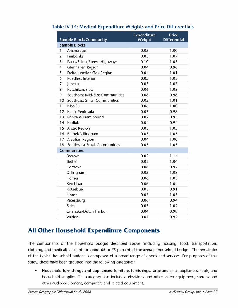
Table IV-14 provides expenditure weights and price differentials for each sample block and selected

community. The price differential for the medical category is the average of the medical services differential

and the medical insurance differential (1.00 for all sample blocks).

See table next page


Table IV-14: Medical Expenditure Weights and Price Differentials


Weight Price

Differential Sample Blocks 1 Anchorage 0.05 1.00 2 Fairbanks 0.05 1.07 3 Parks/Elliott/Steese Highways 0.10 1.05 4 Glennallen Region 0.04 0.96 5 Delta Junction/Tok Region 0.04 1.01 6 Roadless Interior 0.05 1.03 7 Juneau 0.05 1.03 8 Ketchikan/Sitka 0.06 1.03 9 Southeast Mid-Size Communities 0.08 0.98 10 Southeast Small Communities 0.05 1.01 11 Mat-Su 0.06 1.00 12 Kenai Peninsula 0.07 0.98 13 Prince William Sound 0.07 0.93 14 Kodiak 0.04 0.94 15 Arctic Region 0.03 1.05 16 Bethel/Dillingham 0.03 1.05 17 Aleutian Region 0.04 1.00 18 Southwest Small Communities 0.03 1.03 Communities


All Other Household Expenditure Components

The components of the household budget described above (including housing, food, transportation,

clothing, and medical) account for about 65 to 75 percent of the average household budget. The remainder

of the typical household budget is composed of a broad range of goods and services. For purposes of this

study, these have been grouped into the following categories:

• Household furnishings and appliances: furniture, furnishings, large and small appliances, tools, and

household supplies. The category also includes televisions and other video equipment, stereos and

other audio equipment, computers and related equipment.


• Communications: telephones/cell phones and related services, Internet services, cable TV, postage

and delivery services.

• Recreation and education: sporting goods, toys, reading materials (newspapers and magazines),

photography. Also includes pet food and supplies, tuition and related fees, and child-care services.

• Personal care and other: personal-care products and services, laundry services, legal and financial

services. Other includes tobacco and alcohol.

The HCS did not collect data relevant to these spending categories and limited RPS data was collected to

support the analysis of cost differentials.

Weighting (to reflect relative importance in the household budget) of various components within this

category was accomplished by weighting each component in the same proportion as those components

occur in the Anchorage Consumer Price Index (CPI). For example, CPI data indicates that this category

accounts for approximately 22 percent of the after-tax household budget in Anchorage. Within the category,

about one-third (32 percent) of the budget is for household furnishings and appliances, 13 percent for

communication, 33 percent for recreation and education, and 22 percent for personal care and other.

Regardless of how much of a community’s average household budget was captured by the HCS, the un-

captured portion was distributed among the “all other” subcategories according to these percentages. Table

IV-15 illustrates this methodology.

Table IV-15: Estimation of Expenditure Weights in Spending Categories not Measured in the HCS

(Hypothetical Sample Block where 30 percent of Household Budget was not captured in HCS)

Relative Importance from CPI Anchorage

Data

Relative Importance within “All Other”

Category

“All Other” Subcategory Expenditure Weights for

Sample Block

Household furnishings/ appliances 7% 32% 9.6%

Communication 3 13 4.0

Recreation/education 7 33 9.8

Personal care/other 5 22 6.7

Total all other 21% 100% 30%

For calculation of price differentials in the “all other” category, the RPS collected prices for 23 items in the

household furnishings and appliances category, seven communications services, and nine personal care

items. The RPS also collected prices for one brand of cigarettes, seven different drinks at a bar and six alcohol

items for consumption at home.

The communication price differential was calculated as the average of the monthly cost of basic and preferred

cable (or satellite), Internet dial-up, Internet-DSL, phone, long distance rate per minute (in-state), and

monthly wireless. If a particular service was not available in a community, that service was not included in

the average.

Calculating the price differential for the recreation/education category was a two-step process. First, a

recreation price differential was calculated as the average (unweighted) of price differentials for food (to

account for pet food), clothing (proxy for toys, reading material, small sporting goods) and appliances (proxy

for larger sporting good items). The price differential for education was set at 1.00 for all sample blocks and


communities, as identifying a meaningful education market basket suitable for Alaska communities was

considered by the study team to be impractical.

The second step in calculating the price differential for the recreation/education category was to calculate the

average of the recreation component and the education component, with recreation weighted at two-thirds

and education at one-third.

The price differential of the personal care/other subcategory is the weighted average of the personal care

market basket in the RPS (excluding tobacco), tobacco, and alcohol, weighted personal care 60 percent,

alcohol 25 percent, and tobacco 15 percent. In dry communities, alcohol was not included in the average.

Table IV-16 provides expenditure weights and price differentials for the “all other” category.

Table IV-16: All Other Expenditure Weights and Price Differentials


Weight Price

Differential Sample Blocks 1 Anchorage 0.28 1.00 2 Fairbanks 0.25 1.05 3 Parks/Elliott/Steese Highways 0.29 1.06 4 Glennallen Region 0.23 1.02 5 Delta Junction/Tok Region 0.31 1.09 6 Roadless Interior 0.33 1.43 7 Juneau 0.32 1.14 8 Ketchikan/Sitka 0.29 1.15 9 Southeast Mid-Size Communities 0.30 1.21 10 Southeast Small Communities 0.34 1.20 11 Mat-Su 0.27 1.01 12 Kenai Peninsula 0.28 1.05 13 Prince William Sound 0.28 1.11 14 Kodiak 0.27 1.06 15 Arctic Region 0.34 1.50 16 Bethel/Dillingham 0.34 1.38 17 Aleutian Region 0.29 1.40 18 Southwest Small Communities 0.34 1.53 Communities



Note on Subsistence-Related Activity

Subsistence harvests are a critically important part of many households’ budgets. Within the framework of

this study, the cost of subsistence activity is captured in the categories of transportation (vehicles and fuel),

furnishings and appliances (outdoor equipment and supplies), and recreation (which includes “sporting

goods”). The HCS asked for the percentage of household food supply obtained from activities such as

hunting, fishing, gardening or berry-picking. The results of that question for each sample block are provided

in the following table.

While subsistence activity was not factored into the differentials for each GDP, it reinforces the wide variations

in expenditures related to food, transportation and recreation activities.

Table IV-17: Importance of Hunting, Fishing, Gardening, and Gathering in Household Food Supply

Sample Block None Less than

25% 25% to

50% 51% to

75% More

than 75% 1 Anchorage 37% 41% 18% 3% 1% 2 Fairbanks 30 44 19 4 1 3 Parks/Elliott/Steese Highways 26 40 17 15 2 4 Glennallen Region 10 28 28 20 14 5 Delta Junction/Tok Region 12 41 24 17 5 6 Roadless Interior 2 18 31 35 12 7 Juneau 37 45 13 3 2 8 Ketchikan/Sitka 27 46 21 5 2 9 Southeast Mid-Size

Communities 9 48 22 13 2

10 Southeast Small Communities 12 27 31 21 6 11 Mat-Su 27 34 28 7 4 12 Kenai Peninsula 15 46 31 7 2 13 Prince William Sound 13 37 33 12 3 14 Kodiak 13 32 39 10 3 15 Arctic Region 14 32 27 19 7 16 Bethel/Dillingham 12 30 28 21 7 17 Aleutian Region 25 39 30 5 1 18 Southwest Small Communities - 17 32 31 18

section iv: methods and analysis - alaska

Documents