1

Section 7.3 Nested Design for Models with Fixed Effects, Mixed Effects and Random Effects

1052 Part Five MII/li-FlIclor SUIl/il's

23.3

presentation of the variance-covariance matrix in Table 25.4b. In this presentation t rows and four columns are represented by a block matrix. Because of the symmetry ~f ~ur blocks, only two dillerent block matrices are required. These are shown in Table 25.4~ Note the correlations between pairs of observations on the block main diagonal and the uncorrelatedness elsewhere.

Comment

The reason why the restricted mixed model in (25.42) is somewhat more general than the unrestricted model is that two observation~ from the same random factor B level can be positively or negatively correlated for the restricted model according to (25.46b) but cannot be negatively correlated for the unrestricted model. •

Two-Fac10r StlLdies-A~OVA Tf'sts for Models II aud III For both the mixed and random AN OVA models for two-factor studies, the analysis of variance calculations for sums of squares are identical to those for the fixed ANOVA model. Thus, formulas (19.37) and (19.39) are entirely applicable for two-factor ANOVA models II and III. Similarly, the degrees of freedom and mean squares are exactly the same as those shown in Table 19.8 for the fixed two-factor ANOVA model. The random and mixed ANOYA models depart from the fixed ANOYA model only in the expected mean squares and the consequent choice of the appropriate test statistic.

Expected Mean Squares

TABLE 25.5

Mean Square

MSA

MSB

The expected mean squares for the random and mixed ANOYA models for balanced two­factor studies can be worked out by utilizing the properties of the model and applying the usual expectation theorems. They are shown in Table 25.5, together with those for the fixed ANOVA model. The derivations are tedious, but simple rules have been developed for finding the expected mean squares. These rules are described in Appendix D.

Expected Mean Squares for Balanced Two-Factor ANOVA Models.

Fixed AN OVA Model Random ANOVA Model Mixed ANOVA Model df (A and B fixed) (A and B random) (A fixed, B random) .

LIX2 a 2 + nba; + na;fJ

2 LIXl 2 0-1 a 2+nb--; a + nb--

1 + naaP 0- 0-

L{3? b-1 2 J

a +nob

_1

a 2 + noaJ + na;fJ a 2 + noaJ

L L(IX{3)li a 2 + na;fJ a 2 + na;fJ MSAB (0-1)(b-1) a 2 +n

(0-1)(b-1)

MSE (n-1)ob a 2 a 2 a 2

Chapter

---Nested Designs, Subsarnpling, and Partially Nested Designs

In this chapter, we take up the basic elements of nested designs, including the Use of subsampling. We begin by considering the general concept of nested designs and describe how these designs differ froln crossed designs. We then take up in detail two-factor nested designs and their analysis. We conclude by considering subsampling designs and partially nested designs.

26.1 Distinction between Nested and Crossed Factors

Example 1

1088

In the factorial studies considered so far, where every level of one factor appears with each level of every other factor, the factors are said to be crossed. A different situation occurs when factors are nested. The distinction between nested and crossed factors will now be illustrated by some examples involving two-factor studies.

A large manufacturing company operates three regional training schools for mechanics, one in each of its operating districts. The schools have two instructors each, who teach classes of about 15 mechanics in three-week sessions. The company was concerned about the effect of school (factor A) and instructor (factor B) on the learning achieved. To investigate these effects, classes in each district were formed in the usual way and then randomly assigned to one of the two instructorf> in the school. This was done for two sessions, and at the end of each session a suitable summary measure of learning for the class was obtained. The results are presented in Table 26.1.

The layout of Table 26.1 appears identical to an ordinary two-factor investigation, with two observations per cell (see, e.g., Table 19.7). In fact, however, the study is not an ordinary two-factor study. The reason is that the instructors in the Atlanta school did not also teach in the other two schools, and similarly for the other instructors. Thus, six different instructors were involved. An ordinary two-factor investigation with six different instructors would have consisted of 18 treatments, as shown in Figure 26.1 a. In the training school example, however, only six treatments were included, as shown in Figure 26.1 b, where

.'BLE 26.1 Ii : ii¢tple Data ":'Nested ~.,

" o:Factor

ludy­"iliDing

SChool ~ple(class

'lelll1liDg scores, coded).

,:::-.~ . '

SEIGURE 26.1 ·:~inustration \6t:Crossed '~1II1d Nested .---;/,

, Factors­iTraining

::.<School ; i!:xample.

.~,-

Factor A (school)

Atlanta

Average

Chicago

Average "\

r":"~

San fran,ci~co

Average

School (factor A)

Atlanta

Chicago

San Francisco

School (factor A)

Atlanta

Chicago

San Francisco

Chapter 26 Nested Designs, Subsampling, and Partially Nested Designs 1089

~actor B' (inStructor) ( ','

1 2

2~ 14 29 11

Y,1' = 27 Y,2. = 12.5'

11 22 Is ~, .18

Y21' = 8.5 Y22. =20

17 5, 20 2

)131' = 18;5 ~2.=3;5

AVerage

(a) Crossed Factors

Instructor (factor 8)

1 2 3 4 5 6

(b) Nested Factors

Instructor (factor 8)

2 3 4 5 6

Average

)12" =14.25

Yj .. = 11.00

Y." •• =,15

the crossed-out cells represent treatments not studied. Figure 26.2 contains an alternative graphic representation of the nested design for the training school example, including the two replications ofthe study.

It is clear from Figure 26.1 b that the experimental design for the training school example involves an incomplete factorial arrangement of a special type, where each level of factor B (instructor) occurs with only one level offactor A (school). Specifically here, each instructor

1090 Part Six

FIGURE 26.2

School (i)

Instructor (j)

Class (k) (k

Example 2

Specillli:"d SUIlI." [)esiglls

1

Graphic Representation of Two-Factor Nested Design-Training School Example.

12 3 (i = 1) (i = 2) (i = 3)

1 2 3 4 5 (j = 1) (j = 2) (j = 1) (j = 2) (j = 1)

6 (j = 2)

2 3 4 5 6 7 8 9 10 11 = 1) (k = 2) (k = 1) (k = 2) (k = 1) (k = 2) (k = 1) (k = 2) (k = 1) (k = 2)

12 (k = 1) (k= 2)

"- '-'

teaches in only one school. Factor B is therefore said to be nested within factor A. As noted earlier, in an ordinary factorial study where every factor level of A appears with every factor level of B, factors A and B are said to be cmssed.

There is another way to look at the distinction between nested and c!"Ossed designs. Let flij denote the mean response when factor A is at the ith level and factor B is at the jth level. If the factors are cmssed. the jth level of B is the ~ame for all levels of A. If, On the other hand, factor B is nested within factor A. the jth level of B when A is at level I has nothing

in common with the jth level of B when A is at level 2. and so on. For instance, in a crossed factorial study of the effects of price ($1.99, $2.49) and advertising level (high, low), a particular advertising level is the saine no matter with which price it appears, and similarly for the price levels. On the other hand, in the nested design for the training school example, the first instructor in school I is not the saine as the first instructor in school 2, and so On.

An analyst was interested in the effects of community (factor A) and neighborhood (factor B)

on the spread of information about new pmducts. Information was obtained f!"Om samples offamilies in various neighborhoods within selected communities. Since the neighborhood designated I in a given community is not the same as the neighborhoods designated I in the other communitie~. and similarly for the other neighborhoods. neighborhoods here are nested within COllllnUnities.

Comments

I. The distinction between crossed and nested factors is often a fine one. In Example 2, if the neighborhoods of each tommunity represented specilied average income levels so that, say, the firsl neighborhood~ in each community had an average income of $5,000-$9.999. the second neighbor­hoods an average income of$1 0,000-$19.999, and so on for the other neighborhoods. one could view the design as a crossed one. The factors would be community and economic level of neighborhood, Hnd these would be crossed since a given economic level is the same for all communities, and vice . versa.

2. Nested factors are frequently encountered in observational studies where the researcher cannot manipUlate the factors under study. or in experiments where only some factors can be manipulated. Factors that cannot be manipulated. it will be recalled. arc designated observational ti.lctorS, in dis­tinction to experimental factors that can be assigned at will to the experimental units. Example 2 is an observational study wbere both community and neighborhood arc observational factors since f,unilies (the study units) were not randomly assigned to either community or neighborhood. [n Example I, school is an observational factor because the classes of a school (the experimentHI units) are made

1092 Part Six S/Jecialb'd Stud\- Oesigl/s

It follows from (26.4) and (26.1) that:

L!Jj(i) =0

j

1=1. ... ,a (26.5)

The meaning of (3 jlil can be seen 1110st clearly from (26.4). With reference to the tl" . h I I R . . I h d'ff' . hi' allllllg sc 00 exatnp e, f' j(il IS sllnp y tel erence 111 t e mean earning score forthe jth inst

of school i and the average of the mean learning scores for all instructors in that scr:tor

Thus. the effect of the jth instructor in the ith school is measured with respect to the 001 I · . h hi' h' h h . h overall mean earnll1g score for t esc 00 In W IC t e Instructor teac es. We shall call f3_. h

.Ipec(fic efFect of the jth level of factor B nested within the ith level of factor A. J(I) t e We have now expressed the mean respon,;e fJ-iJ in term~ of the overall mean, the mai

effect of the ith level of factor A, and the specific effect of the jth level offactor B neste: within the ith level of factor A, as can be seen from (26.4a):

fJ-;j == fJ- •. + ai + {3jlil == fJ- .. + (fJ-i· - fJ- .. ) + (fJ-lj - fJ-i.) (26.6)

For the training school example. the mean learning score for the jth instructor in school i has been expressed in terms of the overall mean, the main effect of school i, and the specific effect of instructor j within school i.

To complete the model, we need only add a random error term C;Jk.

Nested Design Model Let Y;jk denote the response for the kth trial when factor A is at the ith level and factor B is at the jth level. We assume that there are n replications for each factor level combination, i.e., k = L ... , /7, and that i = I, ... , a and j = I, ... , h. Such a study is said to be balanced because the same number of factor B levels is nested within each factor A level and the number of replications is the same throughout.

When both factors A and B have fixed effects, an appropriate nested design model is:

where:

fJ- .. is a constant

a; are constants subject to the restriction La; = 0

{3j(i1 are constants subject to the restrictions Lj (3j(i) = 0 for all i

Cijk are independent N (0. a 2)

i= I, ... ,a;j= I, ... ,b;k= 1,,, .. /7

(26.7)

The expected value and variance of observation Yijk for nested design model (26.7) with fixed factor effects are:

E {Yi.id = fJ- .. + ai + (3j(i)

a2 {Y;jd = a

2

(26.8a)

(26.8b)

Thus, all observations have a constant variance. Further, the observations YiJk are indepen­dent and norl11all y distributed for this model.

.<

Chapter 26 Nested Designs, Subsampling, and Partially Nested Designs 1093

Comments 1. It is not necessary, as in model (26.7), that the study be balanced, that is, that the number of

replications be,equal for all factor combinations and that the number of levels of nested factor B (number of instructors in the training school example) be the same for each level of factor A (school in this example). We shall discuss the removal of some of these restrictions in Section 26.6. We only point out now that the computations become more complex when the study is unbalanced.

2. There is no interaction term in nested design model (26.7). There is no need for it since factor B is nested within factor A, not crossed with it. To put this somewhat differently, with reference to the training school example, it is not possible to estimate a school-instructor interaction when each instructor teaches in only one school. The teacher effect {3J(i), since it is specific to a given school i, in a sense incorporates the interaction effect between the particular teacher j (in the ith school) and the ith school, but it is not possible in a nested design to disentangle this interaction effect.

3. The factor level means Mi. in a nested design are not generally the same as the corresponding means in a crossed design. Remember that in a nested design, the Mi' are obtained by averaging over only some of the distinctive levels of factor B. With reference to the training school example, the Mi. are obtained by averaging over only those teachers who instruct in the ith school. In a crossed design, on the other hand, the Mi' would be obtained by averaging over all instructors included in the study .

• JSandom Factor Effects

If both factors A and B have random factor levels, nested design model (26.7) is modified

with ai, fJj(i), and Cijk being independent normal random variables with expectations 0 and variances a~, ai, and 0'2, respectively. Thus, it is assumed that all fJj(i) have the same variance al- The assumption that all fJj(i) have the same variance also is made if only factor B is random. It is important to check whether this assumption is appropriate, since it may well be that the mean responses Mil, Mi2, ... , in one factor A level (plant, school, city,

etc.) differ in variability from those in other factor A levels (other plants, schools, cities,

etc.). Tests for equality of variances are discussed in Section 18.2.

26.3 Analysis of Variance for Two-Factor Nested Designs

;Fitting of Model The least squares and maximum likelihood estimators of the parameters in nested design

model (26.7) are obtained in the usual fashion. Employing our customary notation for

sample data in factorial studies, the estimators are:

Parameter Estimator

M·· fL .. = Y. ..

D!; a; = Y; .. - Y. ..

{3j(i) ~j(i) = Y;j. - Y; ..

The fitted values therefore are:

Yjjk = Y .. + (li·. -'Y .. ) + (f;j. - li .. ) = lij· and the residuals are:

(26.9a) (26.9b) (26.9c)

(26.10)

(26.11)

1094 Part Six Specialized Sflldy Designs

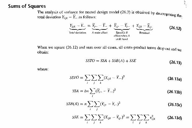
Sums of Squares The analysis of variance for nested design model (26.7) is obtained by decom '

tal d .. v -Y. 'Ii II " POSIng the' to eVIauon 1 ijk - ... as 0 ows.

Yijk - Y. .. = Y; .. - P. .. + Y;j. - Y; .. + Yijk - Y; .. '--v--' '--v---" '--v--' ~ Total deviation A main ctTccl Specific B

effect when A al ilh level

Residual

(26.12)

When we square (26.12) and slim over all cases, all cross-product terms drop out and w obtain: e

where:

SSTO = SSA + SSB(A) + SSE

SSTO = LLL(Y;jk - y' .. )2 j

" - - 2 SSA = bn LUi .. - Y...)

SSB(A) = n L L(Y;]' - Y; .. )2 j

j k

(26.13)

(26.13a)

(26.13b)

(26.13c)

(26.13d) j

SSTO is the usual total slim of squares, and SSA is the ordinary factor A sum of squares, reflecting the variability of the estimated factor level means Y; .. ,

SSB(A) is the factor B sum of squares, with the notation reflecting that factor B is nested within factor A. SSB(A) is made up of terms such as:

n L(Y;j' - Y; .. )2 j

(26.14)

The tenp. in (26.14) is simply the ordinary factor B sum of squares when factor A is at level i. These terms are then summed over all levels of factor A.

Finally, the error sum of squares SSE is, as lIsual, the slim of the squared residuals and reflects the variability of each observation Yijk around the corresponding estimated treatment mean Y;j .. Alternatively, we can view SSE as being made up of terms such a<;:

L L(Y(ik - Y;j.)2

j

(26.15)

The term in (26.15) is simply the ordinary error sum of squares within the ith level of factor A. These terms are then slimmed over all levels of factor A.

Thus, a nested two-factor design can be viewed as a seties of single-factor investigations at the successive levels of the other factor. In terms of the training school example, a study of the effects of instructors (B) within any given school (Ai) leads to the usual sums of squares for instructors and errors in a single-factor analysis of variance within school A,

1096 Part Six Spec;ali:::ed Stl/dy Desigl/s

TABLE 26.3 ANOVA Table for Nested Balanced Two-Factor Fixed Effects Model (26.7) (B nested within A).

Source of Variation 55 elf M5 ~

Factor A SSA = bnL(Y;-- - y' __ )2 0-1 MSA 2 La? a +bn~_

0-1

Factor B (within A) SSB(A) = nLL(Y;j- - Y;-Y 0(b-1) MSB(A) LL{32.\

2 j(b~' a + n----:-:-------.'

Error

Total

FIGURE 26.3 Dot Plots of Class Learning Scores­Training School Example.

SSE = LLL(Yjjk - Y;iY

ssm = LLL (Yijk - y' __ )2

San Francisco (i = 3) o 0

o ~ Chicago (i = 2) u Vl

o o

Atlanta (i = 1)

ob(n-1)

obn-1

o 0

o 10 20 30 Learning Score

MSE

o Instructor j = 1

.. Instructor i = 2

a(b-l~

a 2

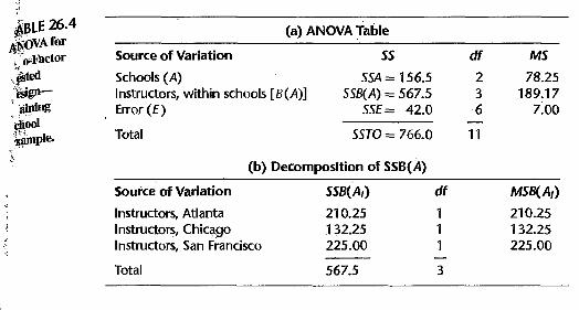
To analyze the instructor and school effects formally, we begin by obtaining the analysis of variance_ The sums of squares were obtained as follows using formulas (26_13):

SSTO = (25 - 15)2 + (29 - 15)2 + ---+ (2 - 15f = 766

SSA = 2(2)[(19-75 - 15)2 + (14_25 - 15)2 + (11.00 - 15)2] = 156_5

SSB(A) = 2[(27 - 19_75)2 + (12-5 - 19_75)2 + ---+ (3_5 - 11.00)2] = 567_5

SSE = (25 - 27)2 + (29 - 27)2 + ---+ (2 - 3_5)2 = 42

Table 26.4a contains the analysis of variance_

Comment

Most analysis of vru-iance computer packages provide an option for obtaining the ANOVA.rfor nested designs_ Should this option be unavailable, the ordinary ANOVA for crossed factors can be used with only slight inconvenience when the nested study is balanced_ SSTO, SSA, and SSE with the crossed-factor analysis will be the same, and SSB(A) is obtained fi-om the relation:

SSB(A) = SSB + SSAB '--v---' '---,....-'

Nested Crossed

The same relation holds for the associated degrees of freedom_

(26.16)

•

,

!j3LE 26.4 ~OVAfor ~'(,.;Factor ~;ted ,es :;~gn­, aiDing "diool ~ple.

~ .

. :-

Chapter 26 Nested Designs, Subsampling, and Partially Nested Designs 1097

(a) ANOVA Table

Source of Variation

Schools (A) Instructors, within schools [B(A)] Error (E)

Total

SS

SSA = 156.5 SSB(A),= 567.5

SSE= 42.0

SSTO= 766.0

(b) Decomposition of SSB(A)

Source of Variation

Instructors, Atlanta Instructors, Chicago Instructors, Scm Francisco

Total

210.25 132.25 225.00

567.5

df MS

2 78.25 3 189.17 6 7.00

11

df MSB(AJ)

1 210.25 1 132.25 1 225.00

3

: Tests for Factor Effects , ..

Tests for factor effects in a nested two-factor study are straightforward. The appropriate test statistics are determined, as for a crossed two-factor study, by comparing the expected values of the ANOVA mean squares. The expected mean squares for nested fixed effects model (26.7) are shown in Table 26.3. They can be obtained by somewhat tedious derivations. We do not illustrate these derivations because Appendix D describes a relatively simple method of finding expected mean squares for any balanced nested design. Also, many computer packages provide the expected mean squares for nested models.

The E{MS} column in Table 26.3 indicates that for fixed effects model (26.7), the test for factor A main effects:

is based on the test statistic:

Ho: all exi = 0

Ha: not all exi equal zero

F* = MSA MSE

and the decision rule to control the level of significance at ex is:

If F* .:::: F[1 - ex; a - 1, (n -1)ab], conclude Ho

If F* > F[1 - ex;a - 1, (n - l)ab], conclude Ha

Similarly, to test for factor B specific effects:

the appropriate test statistic is:

Ho: all {3j(i) = 0

Ha: not all {3 j(i) equal zero

F* = _M_SB_(_A_) MSE

(26.17a)

(26.17b)

(26.17c)

(26.18a)

(26. 18b)

rABLE 26.5 ;j;;gpected Mean isguares for Nested Balanced lwo-Factor IJ)esigns with l{audom FacfOC Effects (Bnested mtbinA).

Mean Square

MSA

MSB(A)

MSE

Test for

Factor A Factor B(A)

Chapter 26 Nested Designs. Subsampling. and Partially Nested Designs 1099

Expected Mean Square

A Fixed, B Random

2:)x? (52 +bn--' + na2

0-1 , fJ

(52 + nai fJ

A Random, B Random

Appropriate Test Statistic

A Fixed, B Random

MSA/MSB(A) MSB(A)/MSE

A Random, B Random

MSA/MSB(A) MSB(A)/MSE

Random Factor Effects Test statistic (26.17b) for factor A main effects is not appropriate if either or both factor effects are random. Table 26.5 gives the expected mean squares for these cases and also the appropriate test statistics.

26.4 Evaluation of Appropriateness of Nested Design Model

Example

The diagnostic procedures described earlier are entirely applicable for examining whether nested design model (26.7) is appropriate. The residuals in (26.11):

(26.20)

may be examined as usual for normality, constancy of the error variance, and independence of the error terms. In particular, aligned dot pi ots of the residuals for each factor A level may be helpful in examining whether the variance of the error terms is constant for the different factor A levels within which factor B is nested.

Figure 26.4a contains MINITAB aligned dot plots of the residuals for each school for the training school example. These plots are affected by the rounded nature of the data, but they support the appropriateness of the assumption of constancy of the error variance. Fig­ure 26.4b presents a normal probability plot of the residuals. This plot is also affected by the rounded nature of the observations, but does not indicate any gross departure from nor­mality. This conclusion is supported by the coefficient of correlation between the ordered residuals and their expected values under normality, which is .927. These and other diag­nostics (not shown here) support the appropriateness of nested design model (26.7) for the training school example.

Comment

Since there are numerous ties among the residuals in the training school example, the normal probability plot in Figure 26.4b is obtained by plotting each of the tied residuals against the ex­pected value for the mean of the tied order positions and showing the number of tied residuals at that position. •

1100 Part Six Specialized Study Designs

FIGURE 26.4 MINITAB • • Diagnostic I Residual • • Plots- I Training

• School • Example. I I

-2.0 -1.0

1.6

""iij ~

0.0 "0 .;;; OJ a::

-1.6

* -3.2

2

(a) Residual Dot Plots

•

• • I I

0.0 1.0

(b) Normal Probability Plot

-1.6

3

0.0 Expvalue

3

1.6

• I I ATLANTA

• • I I CHICAGO

I I SANFRAN 2.0 3.0

* 2

3.2

26.5 Analysis of Factor Effects in Two-Factor Nested Designs

When factor effects are present in a nested design, estimates and/or comparisons of these effects are usually desired.

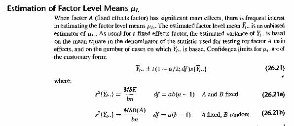
Estimation of Factor Level Means Mi. When factor A (fixed effects factor) has significant main effects, there is frequent interest in estimating the factor level means !Li .. The estimated factor level mean f; .. is an unbiased estimator of !Li .. As usual for a fixed effects factor, the estimated variance of f; .. is based on the mean square in the denominator of the statistic used for testing for factor A main effects, and on the number of cases on which f; .. is based. Confidence limits for p+ are of the customary form:

f; .. ± t(l - a12; df)s{f; .. } (26.21)

where:

2 - MSE s {Yi .. } = -- df = ab(n - 1) A and B fixed

bn (26.21 a)

2 - MSB(A) s {l/ .. } = df = a(b - 1) A fixed, B random

bn (26.21 b)

Confidence limits for contrasts L = LCi!Li., where LCI = 0, are set up in the usual way, utilizing the estimator i = LCi F; .. and the t distribution with degrees of freedom

1102 Part Six Specia/i:ed Study Designs

line plot:

San Francisco Chicago I III GI I

10 ------------- 15 Learning Score

Atlanta lSI

20

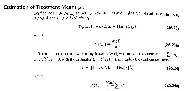
Estimation of Treatment Means {tij

Example

Confidence limits for Ji,ij are set up in the usual fashion using the t distribution when both factors A and B have fixed effects:

1;;. ± tll - a/2; (/1 - l)abls{Y;j.} (26.23)

where:

(26.23a)

To make a comparison within any factor A level, we estimate the contrast L = '" C .11 .. " _ 6 jrlJ'

where Lei = 0, with the estimator L = LcjYij . and employ the confidence limits:

i ± t[l - a/2; (11 - l)ab]s{i} (26.24)

where:

7 ~ MSEL

7 s-{L} = -- C~

n J (26.24a)

The Bonferroni procedure may be used when several comparisons are to be made and the family confidence level is to be controlled. The Tukey procedure is also applicable for paired comparisons and the Schetfe procedure for contrasts, but these procedures often will not be efficient since ordinarily only comparisons within each factor level are of interest, whereas the Tukey and Schetfe families are based on compatisons among all ab treatments.

[n the training school example, we are to compare the mean scores for the two instructors in each school, using the Bonferroni procedure with a 90 percent family confidence coefficient. For g = 3 comparisons, we require B = t[ I - .10/2(3); 6] = t (.983; 6) = 2.748. The estimated variance in each case is:

7 ~ 7.00 s-{L} = -2-(2) = 7.0

Hence, Bs{i} = 2.748.J7.Q = 7.27. Obtaining the estimated treatment means Y;j. from . Table 26.1, we find:

7.2 = (27 - 12.5) - 7.27 .::: Ji,11 - Ji,12 .::: (27 - 12.5) + 7.27 = 21.8

-18.8 = (8.5 - 20) - 7.27 .::: fJ.21 - fJ.22 .::: (8.5 - 20) + 7.27 = -4.2

7.7 = (18.5 - 3.5) -7.27 .::: Ji,31 - Ji,n .::: (18.5 - 3.5) + 7.27 = 22.3

It is evident that substantial differences between the two instructors exist at each school.

,

, '. Chapter 26 Nested Designs, Subsampling, and Partially Nested Designs 1103 ~

~imation of Overall Mean M .. , Sometimes there is interest in estimating the overall mean Ji, •• , For the training school " example, Ji, •• is the overall mean learning score for all training schools and all instructors

in these schools. The point estimator is Y. ... The confidence limits are constructed utilizing ,1 the t distribution as follows:

Y. .. ± t(l - a12; df)s{Y. .. } (26.25)

where:

..,. MSE s2{y. .. } =--

abn df = ab(n -1) A and B fixed (26.25a)

, MSA

s2{y. .. } abn

df=a-l A and B random (26.25b)

s2{y. .. } MSB(A)

df = a(b -1) A fixed, B random (26.25c) abn

~~xample ~ ".

For the training school example, we wish to estimate the overall mean Ji, .. with a 95 percent confidence interval. The estimated variance (26.25a) is appropriate here since the model involves fixed factor effects. Hence, we obtain:

2 - 7.00 s {f. .. } = U = .583 s{Y. .. } = .764

For confidence coefficient .95, we require t(.975; 6) = 2.447. From Table 26.1, we find y. .. = 15. The desired confidence interval therefore is:

13.1 = 15 - 2.447(.764) S Ji, .• S 15 + 2.447(.764) = L6.9

Estimation of Variance Components With random factor effects, estimates of the variance components may be of interest. No new problems arise for balanced nested designs. For instance, we see from Table 26.5 that when both factors A and B are random factors, the variance component a; can be expressed as follows:

2 E{MSA} - E{MSB(A)} a = ---------

ex bn (26.26)

Hence, an unbiased estimator of a; is: 2 MSA - MSB(A)

s =------CI bn

(26.27)

Approximate confidence intervals for variance components a; or a# can be obtained using the MLS interval (25.34). For example, to estimate a; when both A and B are random factors, we see from (26.26) that the correspondences to (25.32) are:

1 c,=­

bn 1

C2=-­bn

MS, =MSA

MS2 = MSB(A)