section 6.3: discrete random variable applications · section 6.3: discrete random variable...

Section 6.3: Discrete Random Variable

Applications

Discrete-Event Simulation: A First Course

c©2006 Pearson Ed., Inc. 0-13-142917-5

Discrete-Event Simulation: A First Course Section 6.3: Discrete Random Variable Applications 1/ 22

Section 6.3: Discrete Random Variable Applications

Example 6.3.1: The inventory demand model in program sis2

The demand per time interval is an Equilikely(10,50) randomvariate

µ = 30, σ =√

140 ∼= 11.8, and the demand pdf is flat

10 20 30 40 500

0.05

0.10

f(d)

d

This model is not very realistic (see Chapter 9)


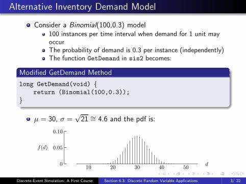
Alternative Inventory Demand Model

Consider a Binomial(100,0.3) model100 instances per time interval when demand for 1 unit mayoccurThe probability of demand is 0.3 per instance (independently)The function GetDemand in sis2 becomes:

Modified GetDemand Method

long GetDemand(void) {return (Binomial(100,0.3));

}

µ = 30, σ =√

21 ∼= 4.6 and the pdf is:

10 20 30 40 500

0.05

0.10

f(d)

d


Example 6.3.2: A Poisson(30) Model

Recall that Binomial(n, p) ≈ Poisson(np) for large n

If Binomial(100, 0.3) is realistic, should also consider Poisson(30)

The function GetDemand in program sis2 would be


long GetDemand(void) {return (Poisson(30.0));

}

µ = 30, σ =√

30 ∼= 5.5 and the pdf has slightly ”heavier” tails

10 20 30 40 500

0.05

0.10

f(d)

d

Poisson(λ) is the inventory demand model used in sis3 with λ = 30


Example 6.3.3: A Pascal(50,0.375) Model

50 instances per time interval

The demand per instance is Geometric(p) with p = 0.375

The function GetDemand in program sis2 would be


long GetDemand(void) {return return (Pascal(50,0.375));

}

µ = 30, σ =√

48 ∼= 6.9 and the pdf has heavier tails than thePoisson(30) pdf

10 20 30 40 500

0.05

0.10

f(d)

d


Example 6.3.4

The number of demand instances per time interval isPoisson(50)

The demand per instance is Geometric(p) with p = 0.375


long GetDemand(void) {long instances = Poisson(50.0); /* avoid 0 */

return (Pascal(instances, 0.375));

}

µ = 30, σ =√

66 ∼= 8.1 and the pdf has heavier tails

10 20 30 40 500

0.05

0.10

f(d)

d


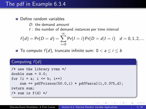
The pdf in Example 6.3.4

Define random variables

D: the demand amountI : the number of demand instances per time interval

f (d) = Pr(D = d) =

∞∑

i=0

Pr(I = i) Pr(D = d |I = i) d = 0, 1, 2, ...

To compute f (d), truncate infinite sum: 0 < a ≤ i ≤ b

Computing f (d)

/* use the library rvms */

double sum = 0.0;

for (i = a; i <= b; i++)

sum += pdfPoisson(50.0,i) * pdfPascal(i,0.375,d);

return sum;

/* sum is f(d) */


Program sis4

Based on sis3 but with a more realistic inventory demandmodel

The inter-demand time is an Exponential(1/λ) random variate

Whether or not a demand occurs at demand instances israndom with probability p

To allow for the possibility of more than 1 unit of demand, thedemand amount is a Geometric(p) random variate

Expected demand per time interval is

λp

(1 − p)


Example 6.3.5: The Auto Dealership

The inventory demand model for sis4 corresponds toλ customers per week on average

Each customer will buy

0 autos with probability 1 − p1 auto with probability (1 − p)p2 autos with probability (1 − p)p2, etc.

With λ = 120.0 and p = 0.2, average demand is 30.0

30.0 =λp

1 − p= λ

∞X

x=0

x(1−p)px = λ(1 − p)p| {z }

19.2000

+2λ(1 − p)p2

| {z }

7.680

+ 3λ(1 − p)p3

| {z }

2.304

+ · · ·

λ(1 − p) = 96.0 customers buy 0 autos

λ(1 − p)p = 19.200 customers buy 1 auto

λ(1 − p)p2 = 3.840 customers buy 2 autos

λ(1 − p)p3 = 0.768 customers buy 3 autos, etc.


Truncation

In the previous example, no bound on number of autospurchased

Can be made more realistic by truncating possible values

Start with random variable X with possible valuesX = {0, 1, 2, . . .} and cdf F (x) = Pr(X ≤ x)

Want to restrict X to the finite range 0 ≤ a ≤ x ≤ b < ∞If a > 0, α = Pr(X < a) = Pr(X ≤ a − 1) = F (a − 1)

β = Pr(X > b) = 1 − Pr(X ≤ b) = 1 − F (b)

Pr(a ≤ X ≤ b) = Pr(X ≤ b) − Pr(X < a) = F (b) − F (a − 1)

Essentially, always true iff F (b) ∼= 1.0 and F (a − 1) ∼= 0.0


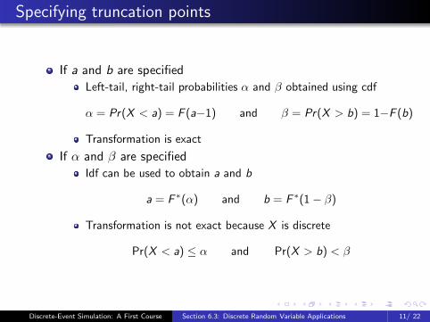
Specifying truncation points

If a and b are specified

Left-tail, right-tail probabilities α and β obtained using cdf

α = Pr(X < a) = F (a−1) and β = Pr(X > b) = 1−F (b)

Transformation is exact

If α and β are specified

Idf can be used to obtain a and b

a = F ∗(α) and b = F ∗(1 − β)

Transformation is not exact because X is discrete

Pr(X < a) ≤ α and Pr(X > b) < β


Example 6.3.6

For the Poisson(50) random variable I , determine a, b so that

Pr(a ≤ I ≤ b) ∼= 1.0

Use α = β = 10−6

Use rvms to compute

Determining a, b

a = idfPoisson(50.0,α); /*α = 10−6*/

b = idfPoisson(50.0,1.0 - β); /*β = 10−6*/

Results: a = 20 and b = 87

Consistent with the bounds produced by the conversion:

Pr(I < 20) = cdfPoisson(50.0, 19) ∼= 0.48 × 10−6 < α

Pr(I > 87) = 1.0 − cdfPoisson(50.0, 87) ∼= 0.75 × 10−6 < β


Effects of Truncation

Truncating Poisson(50) to the range {20, . . . , 87} isinsignificant: truncated and un-truncated random variableshave (essentially) the same distribution

Truncation is useful for efficiency:

When idf is complex, inversion requires cdf searchcdf values are typically stored in an arraySmall range gives improved space/time efficiency

Truncation is useful for realism:

Prevents arbitrarily large values possible from some variates

In some applications, truncation is significant

Produces a new random variableMust be done correctly


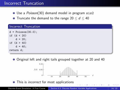
Incorrect Truncation

Use a Poisson(30) demand model in program sis2

Truncate the demand to the range 20 ≤ d ≤ 40

Incorrect Truncation

d = Poisson(30.0);

if (d < 20)

d = 20;

if (d > 40)

d = 40;

return d;

Original left and right tails grouped together at 20 and 40

10 20 30 40 500

0.05

0.10

f(d)

d

This is incorrect for most applications


Truncation by cdf Modification (1)

Example 6.3.8: Truncate Poisson(30) demands to range20 ≤ d ≤ 40

The Poisson(30) pdf is (before truncation)

f (d) = exp(−30)30d

d !d = 0, 1, 2, ...

Pr(20 ≤ D ≤ 40) = F (40) − F (19) =40∑

d=20

f (d) ∼= 0.945817

Compute a new truncated random variable Dt with pdf ft(d)

ft(d) =f (d)

F (40) − F (19)d = 20, 21, ..., 40



The corresponding truncated cdf is

Ft(d) =d∑

t=20

ft(t) =F (d) − F (19)

F (40) − F (19)d = 20, 21, ..., 40

Mean and standard deviation of Dt

µt =40X

d=20

dft(d) ∼= 29.841 and σt =

vuut

40X

d=20

(d − µt)2ft(d) ∼= 4.720

Mean and standard deviation of Poisson(30)

µ = 30.0 and σ =√

30 ∼= 5.477



A random variate truncated to 20 ≤ d ≤ 40 can be generatedby inversion, using the truncated cdf Ft(·) and Alg.6.2.2

Truncation by cdf Modification

u = Random();

d = 30;

if (Ft(d) <= u)

while (Ft(d) <= u)

d++;

else if (Ft(20) <= u)

while (Ft(d-1) > u)

d--;

else

d = 20;

return d;


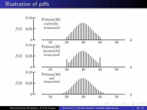
Illustration of pdfs

10 20 30 40 500

0.05

0.10

f(d)

d

Poisson(30)correctlytruncated

10 20 30 40 500

0.05

0.10

f(d)

d

Poisson(30)incorrectlytruncated

10 20 30 40 500

0.05

0.10

f(d)

d

Poisson(30)not

truncated


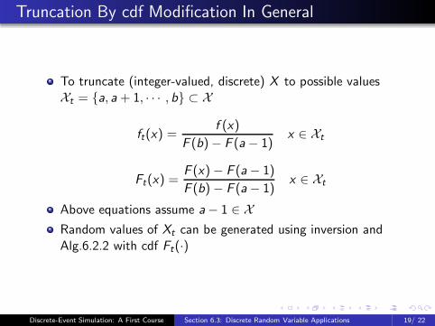
Truncation By cdf Modification In General

To truncate (integer-valued, discrete) X to possible valuesXt = {a, a + 1, · · · , b} ⊂ X

ft(x) =f (x)

F (b) − F (a − 1)x ∈ Xt

Ft(x) =F (x) − F (a − 1)

F (b) − F (a − 1)x ∈ Xt

Above equations assume a − 1 ∈ XRandom values of Xt can be generated using inversion andAlg.6.2.2 with cdf Ft(·)


Truncation by Constrained Inversion

Use the idf of X to generate Xt truncated to a ≤ x ≤ b

Truncation by Constrained Inversion

/* assumes a - 1 is a possible value of X */

α = F(a-1);β = 1.0 - F(b);u = Uniform(α, 1.0 - β);x = F ∗(u); /* F ∗(·) is the idf of X */

return x;

The key is that u is constrained to a subrange(α, 1 − β) ⊂ (0, 1)

Truncation is automatically enforced prior to inversion


Example 6.3.9

Generate a Poisson(30) random demand truncated to20 ≤ d ≤ 40

Example 6.3.9

α = cdfPoisson(30.0, 19); /*set-up*/

β = 1.0 - cdfPoisson(30.0, 40); /*set-up*/

u = Uniform(α, 1.0 - β);d = idfPoisson(30.0, u);return d;

Uses library rvms

α and β are static variables that are computed once only


Truncation By Acceptance-Rejection

Truncate Poisson(30) by using acceptance-rejection

Truncation By Acceptance-Rejection

d = Poisson(30.0);

while ((d < 20) or ( d > 40))

d = Poisson(30.0);

return d;

Acceptance-rejection is not synchronized or monotone even ifthe un-truncated generator has these properties

Truncation by cdf modification or constrained inversion ispreferable


section 6.3: discrete random variable applications · section 6.3: discrete random variable...

Documents