Section 4.1 - Exponential Functions(Part I – Growth) “The number of cars in this city is growing exponentially every year”. You may have heard quotes such as this. Let’s take a look at some other exponential quotes: http://www.brainyquote.com/quotes/keywords/exponentially.html Many of these quotes are not accurate in a mathematical sense. We now investigate the meaning of an Exponential Function in math.

An example of an exponential function is . Notice that the exponent is the variable whereas in a power function, such

as , the base is the variable. Let’s take a look at the

graph of using an x-y table of values.

As x goes up by one, what happens to the y-value?

f (x) 2x

f (x) x2

f (x) 2x

It doubles each time. If we continued the table, we see that the y-value is going up very fast. How does this compare to the growth of other functions we are familiar with? Look at the y-values from left to right in this table.

x 1 2 3 4 5 6 7 8 9 10 11

y = 2x 2 4 6 8 10 12 14 16 18 20 22

y = x 1 4 9 16 25 36 49 64 81 100 121

y= 2 2 4 8 16 32 64 128 256 512 1024 2048

We can see the behavior of the functions on the graph of the 3 functions below. Error:*The red graph is not y=2x It is y=½ x.

So, from the table and graph, we see that an exponential function grows much faster than other functions we have seen.

2

x

x 4 5 6 7

y 16 32 64 128

Definition: An exponential function is a function of the form

. The value b is the base of the exponential function. Why can’t a = 0 in the function? To examine exponential functions further, let’s allow a = 1. We

now have the exponential . Why can’t b = 1? We could let b = 1, but it would just be the useless constant

function , which is not an exponential function at all. Why can’t we have a negative number for b? For example, what happens if we let b = -1?

x 1 2 3 4 5 6 7 8 9 10 11

y = -1 1 -1 1 -1 1 -1 1 -1 1 -1

How useful would this exponential function be to us? What physical quantity could this possible model? In addition, this function is undefined for many x-values in between the integers shown in the table above. Let’s take a look at the graphs of some examples of our

simplified exponential function .

f (x) bx

1 x

f (x) 1

f (x) bx

f (x) abx , a 0, b 0 and b 1

What is the domain and range for each of these functions? Domain: All real numbers Range: y > 0 Are there any asymptotes on the graph? One - horizontal asymptote at y = 0. This is due to the end-

behavior of these functions. As . Remember: Horizontal asymptotes can be derived from examining the end-behavior of a function. What point do all of these graphs have in common? The point ( 0, 1 ). Does this make sense? What does any base to the zeroth power equal to? One.

x or x , f (x) 0

Now, let’s put the a back into the function rule, . Let’s stay with b = 2 and let a = 3. What will happen to the graph of

? The new function would be written as, . How about with b = 2 and let a = -1. What will happen to the

graph of ? The transformed function would be written

as, or . What do you think the graphs of the following functions would

look like compared to ?

If the last function seems difficult to figure out, think about what some other functions that you already know would look like:

How do and change in relation to

their parent functions of , ?

The graph of looks identical to a graph we have

already seen,

.

Exponential Growth - .

When a > 0 and b > 1, the exponential function is often referred to as an exponential “growth” function. What this

f (x) abx

f (x) abx , a 0 , b 1

f (x) 1

2

x

f (x) 2x f (x) 2 1x

f (x) 21 x

f (x) 2x

f (x) x2f (x) x

f (x) (3x 3)2f (x) 3x 3

f (x) 23x3f (x) 3(2)x3 4f (x) 2xf (x) 2x3

f (x) 2x

f (x) 2xf (x) (2)xf (x) 2x

f (x) 3(2)xf (x) 2x

f (x) abx

means, graphically, is that as we look at the function from left to right, the function(the y-value that is) is increasing(or growing) quickly at an exponential rate(the y’s are multiplied by the same number). We already saw an example of an exponential growth

function namely . If we look at an x-y table that demonstrates exponential growth, the y-value is always multiplied by the same number when the x-value increases by the same amount. For example, the table to the right is an exponential function with b = 2 and a = 6. An increasing exponential function gets this special “growth” name because it is used to model many real-life situations. Some of the many examples of situations that we can model using an exponential growth function are: 1.) Bacteria growth in an organism 2.) Compound interest in banking 3.) Spread of disease, flu, etc. 4.) Moore’s Law - the number of transistors on integrated circuits(used in computer chips) doubles approximately every two years. 5.) Inflation of the price of goods in an economy 6.) Nuclear fission/chain reaction

Note(Important): Notice in the function rule , if we let x = 0, then f(x) = a. In many exponential functions( or models ) we will investigate, the x will often be changed to “t” which represents the time elapsed since you started

f (x) abx

f (x) 2x

x 0 2 4 6

y 6 24 96 384

something - like measuring the spread of a disease or the time since you initially deposit money in a savings account. We should be able to look at the rule for an exponential function and determine whether it is a growth example and then graph it using an x-y table. *Don’t forget to have negative values for x in your table. If the variable is time( t ), then you probably will not need negative values. Now, you try to do this with the following functions:

and . 1.) Fill out an x-y table going from -3 to 3. *You can use a calculator to fill out your x-y tables. Hint: To get from one y-value to the next one on the table, just multiply by the b in

. 2.) Use your x-y table to get a graph of the function. Solutions:

1.)

f (x) 3(1.5)xf (x) 0.5(2)x

f (x) abx

f (x) 3(1.5)xf (x) 0.5(2)x

x -3 -2 -1 0 1 2 3 4

y 0.06 0.13 0.25 0.5 1 2 4 8

x -4 -3 -2 -1 0 1 2 3

y 0.6 0.9 1.3 2 3 4.5 6.8 10.1

2.)

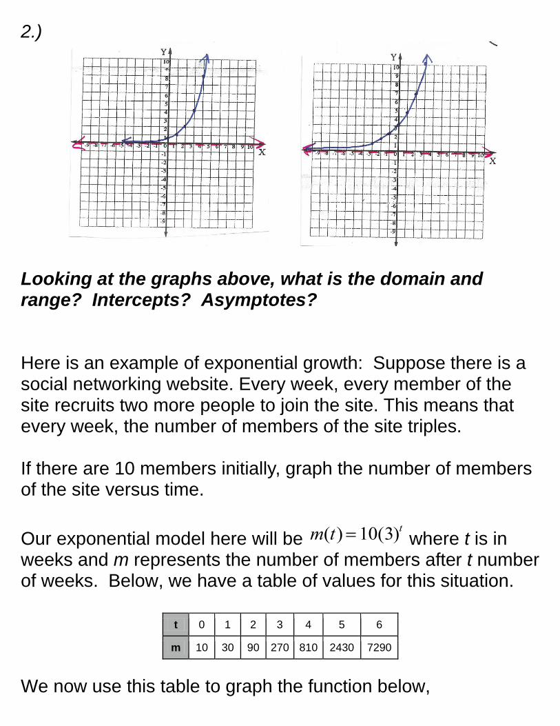
Looking at the graphs above, what is the domain and range? Intercepts? Asymptotes? Here is an example of exponential growth: Suppose there is a social networking website. Every week, every member of the site recruits two more people to join the site. This means that every week, the number of members of the site triples. If there are 10 members initially, graph the number of members of the site versus time.

Our exponential model here will be where t is in weeks and m represents the number of members after t number of weeks. Below, we have a table of values for this situation. We now use this table to graph the function below,

t 0 1 2 3 4 5 6

m 10 30 90 270 810 2430 7290

m(t) 10(3)t

*Calculator Note: When graphing exponential functions, make sure to adjust your window settings( x-min/x-max/y-min/y-max ) in such a way so that you can see the graph. Sometimes the graphs of these functions will not fit the usual scaling. A common way to use exponential growth functions is to speak of how many percent a quantity increases in a given time interval such as a second, minute, month, year, etc. When we use exponential growth in this way, we write the function rule in a slightly different way: Exponential Growth Function(when growth is a percent):

where a is the initial amount of some quantity, 1 + r is the growth factor(or growth rate), and t is the time since you started observing the data. Note: We usually let the beginning time be t = 0, which is when the amount of the quantity will be equal to “a”.

f (t) a(1 r)t

Let’s take a look at some real-world applications problems that use exponential growth as a percent. Example A: In 1980 about 2,180,000 people worked at home in the U.S. During the next ten years, the number of people who worked at home increased by 5% every year. 1.) Write an exponential function which models this situation by giving the number of people working at home t years after 1980. Let w = number of people working at home(in millions).

. *Notice how we can just use 2.18 for a if we let the scaling on the graph be 1. 2.) Use the graph of this function to predict when there will be about 3.22 million people working at home. What scaling should we use for this graph? The scaling looks like it should be x-min = 0, x-max = 12, x-scl = 1; y-min = 0, y-max = 5, y-scl = 1. Let’s do this graph on the graphing calculator. From the graph, we estimate that there will be about 3.22 million people working at home 8 years after the beginning of our data or 1988. Example B : In January 1993 there were about 1,313,000 internet web hosts. An internet web host is a company that provides space on a server they own for use by their clients as well as providing Internet connectivity, typically in a data center.

w(t) 2.18(1 .05)t w(t) 2.18(1.05)t

During the next 5 years, the number of web hosts increased by about 100% per year. 1.) Write an exponential function which models this situation by giving the number of web hosts t years after 1993. Let h = the number of web hosts(in millions).

. Notice how we can just use 1.313 for a if we let the scaling be 1. 2.) Use the model to predict how many hosts there will by the year 1996. From the model, we estimate that there will be about 10.5 million web hosts 3 years after the beginning of our data or 1993 in the year 1996. 3.) Use the graph of this function to predict when there will be about 30 million web hosts. What scaling should we use for this graph? The scaling looks like it should be x-min = 0, x-max = 6, x-scl = 1; y-min = 0, y-max = 40, y-scl = 5. Let’s do this graph on the graphing calculator. From the graph, we estimate that there will be about 30 million web hosts approximately 4.5 years after the beginning of our data or July 1, 1997. Now, you try to do the following problem:

h(t) 1.313(11.0)t h(t) 1.313(2)t

In January 2010, the cost of tuition at a state university was $7,300 per year. During the next 8 years, the tuition is projected to rise 4% each year.

1.) Using , write an exponential function which models this situation. Let c = cost of tuition t years after 2010. 2.) Use the graph of this function to predict when the tuition will reach $8,000.

Answers: 1.) 2.) Using scaling of x-min = 0, x-max = 10, x-scl = 1 and y-min = 0, y-max = 10, y-scl = 1. It looks like the graph is linear, not exponential. Using the trace function, we find that when y = 8, x ≈ 2.34 which means that around ( 0.34 x 12 = 4.08 ) the beginning of April 2012, the tuition will reach $8,000. Another common example of exponential growth is Compound Interest. Compound Interest is used when calculating the interest on loans from banks, interest accrued from borrowing using a credit card, interest accrued on a savings account among other situations. Compound Interest Formula: where A = the amount of interest

A(t) p 1

r

n

nt

c(t) 7.3(1 .04)t c(t) 7.3(1.04)t

c(t) a(1 r)t

accrued, p = the principal(amount of money initially invested or borrowed), r = the annual interest rate usually given in the problems as a percent, n = the number of times interest is compounded per year, t = the number of years that interest has been compounded. Let’s look at a typical compound interest problem, You deposit $1,000 in a savings account that pays 8% interest. Find the balance after 1 year if the interest is compounded: Compound Interest Formula:

a.) annually --> = $1,080

b.) quarterly --> = $1,082.43

c.) monthly --> = $1,083

d.) daily --> = $1,083.28 How much difference did changing the compounding period make?

A(t) p 1r

n

nt

A(t) 1000 1.08

365

3651

A(t) 1000 1.08

12

121

A(t) 1000 1.08

4

41

A(t) 1000 1.08

1

11

*Hmwk: From the problems below, do 2-24 all, 35-41 odd, 43-45 all, 49-51 all, 56-58 all. *For problems 4-9, make sure you have the correct scaling on the y-axis. *For problems 44, 45, 50, 51 you may use a graphing calculator, you do not need to actually show the graph in your homework. *For problems 56-58 use the DESCRIPTIVE variables given in the problem when you are writing your function/model. *You may use a graphing calculator to check any problem that involves graphing.

Below are some answers to some of the odd numbered problems in this assignment.