section 2 chapter 2 - ohio epaepa.ohio.gov/portals/27/atu/section2chapter2.pdf · section 2,...

Section 2, Chapter 2 CHARACTERIZATION OF PM2.5 IN CENTRAL AND SOUTHEAST OHIO

INTRODUCTION

The research presented in this section was conducted to provide a comprehensive study of the chemical and transport characteristics of PM2.5 in urban, suburban, and rural areas of Central and Southeastern Ohio. The main objectives of this research study are:

To determine the levels of PM2.5 in the three counties

representing urban, suburban, and rural areas of Central and Southeastern Ohio;

To chemically characterize PM2.5 in the study areas; To study indoor and outdoor PM2.5 characteristics in the study

areas; To study the relationship of PM2.5 with ozone and various

meteorological parameters; To study the transport characteristics of PM2.5 in these areas.

Measurements in several urban atmospheric environments have shown an

increasing trend in the concentration of highly dispersed fine aerosols (i.e. aerosols with particle diameters less than 2 µm), and a decrease in the concentration of coarse particles (diameter less than 10 µm).1 Total emissions from transportation, and fuel combustion, etc. make up most of the anthropogenic fine aerosols (size under 2µm) in the ambient atmosphere. The coarse particulates in industrial emissions are efficiently separated by air cleaning equipments. Fine aerosols can be dispersed in the atmosphere homogeneously, can be transported for long distances, and, because of their relatively high residence times in the atmosphere, can accumulate there.

62 PM Characterization

Fine aerosol particles are formed by condensation of hot vapors during the

combustion process and from gas-to-particle conversion in the atmosphere. Because of the small size of PM2.5, they can penetrate deeply into the lungs and result in adverse human health effects. Several studies indicate that increases in human mortality and morbidity are associated with levels of air particulate significantly lower than previously thought.2

In July 1997, the USEPA made changes to the PM National Ambient Air Quality Standards (NAAQS) by adding two new primary PM2.5 standards set at 15 µg/m3 (annual arithmetic mean) and 65 µg/m3 (24-hour average). This change was to provide increased protection against PM-related health effects. Areas will be in compliance with the new annual PM2.5 standard when the 3-year average of the annual arithmetic mean PM2.5 concentrations, from single or multiple community-oriented monitors, is less than or equal to 15 µg/m3. For the new 24-hour PM2.5 standard, the form is based on the 98th percentile of PM2.5 concentrations in one year (averaged over 3 years), at the population-oriented monitoring site with the highest measured values in an area.3

PM2.5 Monitoring

Ambient air monitoring was conducted at the three locations noted in Chapter 1 of this section. A teacher was trained to operate and collect the samples, and calibrate the personal sampling pumps at each of the sites. The School of Health Sciences at Ohio University was in charge of training the teachers as well as measuring the mass of the filters before and after sampling. Ohio University was also responsible for the maintenance and flow calibrations of the monitors.

CHEMICAL CHARACTERIZATION

This section provides background information about the chemical characterization of PM2.5 and the methodology used in the characterization. It documents information about the analytical equipment used for the chemical characterization and the quality assurance and quality control procedures utilized in this study.

Chemical Analysis

The ambient and indoor PM2.5 samples collected on teflon filters were analyzed using X-Ray Fluorescence (XRF) and Ion Chromatography (IC) techniques. Elemental analysis was conducted on the filter samples using a Kevex 771-EDX Spectrometer (Energy Dispersive X-ray Fluorescence) instrument. The PM2.5 mass was analyzed for Silicon, Phosphorus, Sulfur, Chlorine, Potassium, Calcium, Titanium, Vanadium, Chromium, Mangenese, Iron, Cobalt, Nickel, Copper, Zinc, Arsenic, Cadmium and Tin. The filters were subsquently extracted with deionized water by ultrasonic treatment, and

PM Characterization 63

the anions (F-, Cl-, NO3 -, SO4

-2, PO4-3) and cations (LI+, Na+, NH4

+, K+, Mg+2, Ca+2) present were determined using the Dionex DX-500 IC (ion chromatography) system.

Analytical Equipments and Methodology

Continuous ambient PM2.5 measurements were carried out using TEOM Series 1400a monitors manufactured by Ruprecht and Patashnick Co. Inc. The TEOMs were set to run 24–hours, seven days a week. Filter-based ambient PM2.5 measurements were made with an Automatic Cartridge Collection Unit (ACCU) System, which was connected to the TEOMs. The 24-hour averaged filter samples were collected daily during weekdays.

Indoor monitors were operated at 10 L/min using flow-controlled indoor sampling pumps (Model 3000-02Q, URG). Measurements of indoor PM2.5 concentrations were made using 2.5 µm cyclones (URG-2000-30EH). Indoor monitors were timed to run from 8:00 a.m. to 3:00 p.m. Monday through Friday throughout the school year. The ambient outdoor and indoor PM2.5 measurements and monitoring scheme is discussed in detail earlier in this report.

The indoor and outdoor samples were collected on 37 mm and 47 mm Whatman Teflon filters (2-µm pores size), respectively. After the sampling, the filters were placed in Petri dishes, double bagged and kept at 4°C until analysis. Samples were then sent to the Department of Environmental Engineering at Texas A & M University - Kingsville to perform chemical speciation and analysis.

The analysis of trace elements was performed using the Kevex 771-EDX Spectrometer (Energy Dispersive X-ray Fluorescence) instrument. X-Ray Fluorescence is a non-destructive technique that can analyze elements from Fluorine to Uranium in the periodic table. The instrument consists of a spectrometer, secondary targets, Rhodium target x-ray tube and high resolution Si(Li) solid state x-ray detector.4 All filters were run with Germanium as the secondary target with the tube voltage set to 50 kV and the tube current to 2.9 mA. Air was used in the chamber and the counting time was set to 100 seconds. Elements found in the samples included Silicon, Phosphorus, Sulfur, Chlorine, Potassium, Calcium, Titanium, Vanadium, Cromium, Mangenese, Iron, Cobalt, Nickel, Copper, Zinc, Arsenic, Cadmium and Tin.

The particles sampled on the filters were then extracted with deionized

water for 10 minutes using the Fisher Scientific FS9 ultrasonic, and the anions (F-, Cl-, NO3

-, SO4-2, PO4

-3) and the cations (Li+, Na+ , NH4+, K+, Mg+2, Ca+2)

present were determined using the Dionex DX-500 IC (ion chromatography) system. The system included an electrochemical detector, chromatography oven, gradient pump, and an autosampler. This method of analysis is


destructive in nature as the filter samples are dissolved in deionized water and hence lost. The anion guard, column and suppressor assembly is used for the anion analysis and cation guard, column and a suppressor is used to measure the cation concentration in the filter samples. Peaknet 5.0 software is used for the calibration curve generation, post-run data processing, and the report generation.5

Quality Assurance

Quality control (QC) and quality auditing establish the precision, accuracy, and validity of measured values. Quality assurance integrates quality control, quality auditing, measurement method validation, and sample validation into the measurement process. The results of quality assurance are data values with specified precision, accuracy, and validity.6

Quality control is intended to prevent, identify, correct, and define the consequences of difficulties that might affect the precision and accuracy, and or validity of measurements.7 QC activities for Texas A&M- University Kingsville included modifying standard operating procedures followed during ambient sampling/ source sampling, chemical analysis, data processing, and quality auditing.

The quality auditing function consisted of systems and performance audits. The systems audit included a review of the operational and QC procedures to assess whether they were adequate to assure valid data that they met the specified levels of accuracy and precision. It also examined all phases of the measurement activity to determine that procedures were followed and that operators were properly trained. Performance audits established whether the predetermined specifications were achieved in practice. Both system and performance audits were performed at Texas A&M University – Kingsville and Ohio University on an annual basis to assure data quality. In addition, proper maintenance procedures were followed for the equipments in this study for sampling and chemical analysis.

AMBIENT OUTDOOR ANALYSIS

The chemical speciation and analysis of the filter samples was performed at Department of Environmental Engineering at Texas A & M University – Kingsville. The results of ambient outdoor analysis are assembled in this section. First, the data tables provide PM2.5 mass and chemical composition measurements. Then, data is validated and spatial variations of the PM2.5 concentrations and temporal variations of PM2.5 sulfate concentrations are examined.


PM2.5 Mass and Chemical Composition Data Summary

Tables II.2.1 to II.2.3 depict the PM2.5 mass and chemical composition data summary for the three outdoor sites in Ohio for the study period from February 1999 to August 2000. The average PM2.5 mass concentrations considered here are the arithmetic averages of the filter mass collected at each site during the entire period of study.

Sulfate ion was the largest component present in the samples. The average sulfate concentrations were highest at Koebel and lowest at New Albany. Other abundant components present in the samples were silicon, chlorine ion, and sodium ion. The concentrations of these components varied from site to site.

Data Validation The data acquired from field monitoring and laboratory analysis were

compared for consistency. The data was validated by checking the sum of the chemical species concentrations against the total PM2.5 mass. Regression plots were run to examine the relationships between parameters such as the chemical the species concentration and sum of chemical species. Outliers were reexamined to determine the cause of discrepancy. Results from the data validation for the period of May through August 2000 are presented in Figures II.2.1 to II.2.3.

Sum of Chemical Species Versus PM2.5 Mass Concentrations

The measured and monitored mass data were compared by plotting the scatter graphs for the sum of species against mass concentrations. Correlation between these two parameters was studied by plotting the mass concentration (independent variable X) against the sum of species (dependent Y).

Many of the species remain unidentified in the chemical analysis and hence

the sum of the species should always be less than or equal to the gravimetrically measured mass.8 In order to avoid the double counting, total sulfur (S), soluble potassium (K+) and chloride (Cl-) were excluded from the sum of species.

Figures II.2.1 to II.2.3 show a relationship between the measured mass

concentration and the sum of chemically analyzed species. Also, it is clear that the sum of species is always less than the gravimetrically measured PM2.5 mass concentrations.


Table II.2.1. Statistical summary of PM2.5 mass and its chemical compositions at Athens (February 1999-August 2000)

Species Range (µg/m3)

Average Standard Deviation Median

Minimum Maximum PM2.5 Mass 13.66 8.91 11.494 0.50 61.12

Si 0.1124 0.1979 0.0473 0.0005 1.5285 P 0.0018 0.0012 0.0015 0.0001 0.0050 S 0.7130 1.2759 0.3278 0.0022 10.9926 Cl 0.0116 0.0202 0.0046 0.0001 0.1675 K 0.0180 0.0099 0.0161 0.0002 0.0399 Ca 0.0100 0.0215 0.0047 0.0000 0.2529 Ti 0.0010 0.0022 0.0003 0.0000 0.0209 V 0.0002 0.0003 0.0001 0.0000 0.0031 Cr 0.0015 0.0011 0.0010 0.0001 0.0046 Mn 0.0006 0.0009 0.0002 0.0000 0.0041 Fe 0.0062 0.0128 0.0032 0.0000 0.1190 Co 0.0016 0.0014 0.0012 0.0001 0.0050 Ni 0.0007 0.0005 0.0006 0.0001 0.0022 Cu 0.0008 0.0021 0.0001 0.0000 0.0139 Zn 0.0012 0.0023 0.0005 0.0000 0.0209 As 0.0037 0.0026 0.0029 0.0003 0.0118 Cd 0.0001 0.0001 0.0001 0.0000 0.0002 Sn 0.0010 0.0008 0.0008 0.0001 0.0035 Li+ 0.0016 0.0018 0.0005 0.0001 0.0053 Na+ 0.1569 0.3045 0.0631 0.0010 2.7660

NH4+ 0.4824 0.6069 0.1473 0.0000 2.4876 K+ 0.1755 0.2302 0.0562 0.0024 0.9903

Mg+2 0.0765 0.1171 0.0191 0.0012 0.4721 Ca+2 0.1074 0.2369 0.0436 0.0001 1.2395

F- 0.0071 0.0033 0.0053 0.0040 0.0146 Cl- 0.1399 0.1702 0.0438 0.0030 0.7112

NO3- 0.5618 0.6207 0.1911 0.0059 2.2013 PO4

-3 - - - - - SO4

-2 2.5831 2.2836 1.8627 0.0207 9.3761 Sum of Species 5.1777 6.1288 2.8454 0.0421 33.4600

Unidentified 7.7035 2.0095 8.4288 0.4294 27.6557


Table II.2.2. Statistical summary of PM2.5 mass and its chemical compositions at New Albany (February 1999-August 2000)





NH4+ 0.5162 0.5930 0.2472 0.0012 2.6985 K+ 0.1336 0.2113 0.0432 0.0001 1.4805

Mg+2 0.0260 0.0356 0.0231 0.0004 0.3135 Ca+2 0.0818 0.1438 0.0309 0.0001 1.1321

F- 0.0047 0.0010 0.0048 0.0037 0.0059 Cl- 0.2237 0.2607 0.1893 0.0028 1.6247

NO3- 0.2020 0.2772 0.0893 0.0048 1.3209 PO4

-3 0.2265 0.1735 0.1686 0.0340 0.5688 SO4

-2 2.1201 2.0044 1.5139 0.0092 13.7594 Sum of Species 4.5060 4.9841 2.8479 0.0637 31.5071

Unidentified 8.6687 3.4865 8.5798 -0.0115 29.8298


Table II.2.3. Statistical summary of PM2.5 mass and its chemical compositions at Koebel (February 1999-August 2000)





NH4+ 0.5264 0.5332 0.3113 0.0003 2.5725 K+ 0.0997 0.1201 0.0643 0.0006 0.8591

Mg+2 0.0313 0.0850 0.0177 0.0003 0.7842 Ca+2 0.1237 0.1255 0.0794 0.0004 0.6981

F- 0.0518 0.0760 0.0184 0.0044 0.2000 Cl- 0.2401 0.2560 0.2118 0.0104 1.9171

NO3- 0.2591 0.3284 0.0965 0.0080 1.4070 PO4

-3 0.3252 0.4785 0.0928 0.0332 1.6907 SO4

-2 2.7139 2.4591 2.0275 0.0152 13.7931 Sum of Species 5.6608 6.7151 3.5630 0.0864 45.3192

Unidentified 7.8843 1.2591 7.9480 1.4237 13.9203


Figure II.2.1. Scatter plot of sum of species versus mass outdoor concentrations for Athens (May- August 2000)

Figure II.2.2. Scatter plot of sum of species versus mass outdoor concentrations for New Albany (May-August 2000)

y = 0.3078x + 0.8263R = 0.85

02468

10121416

0 10 20 30 40 50

PM2.5 Mass (ug/m3)

Sum

of S

peci

es (u

g/m

3 )

y = 0.2827x + 1.0284R = 0.84

02468

10121416

0 10 20 30 40

PM2.5 Mass (ug/m3)

Sum

of S

peci

es (u

g/m

3 )


Figure II.2.3. Scatter plot of sum of species versus mass outdoor concentrations for Koebel (May-August 2000)

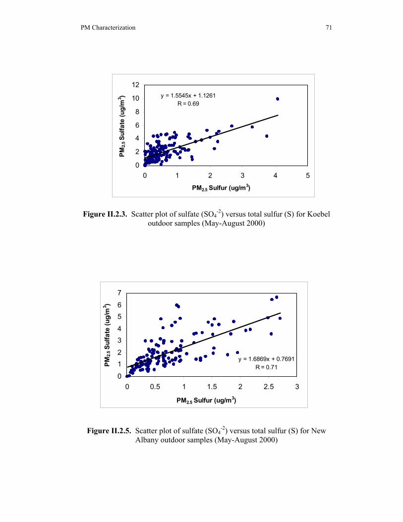
Sulfate versus Total Sulfur

Sulfate (SO4-2) ion concentration was obtained by ion chromatography (IC)

analysis and the total sulfur (S) concentration was obtained from x-ray fluorescence (XRF) analysis on Teflon-membrane filters. Figures II.2.4 to II. 2.6 show scatter plots of sulfate versus sulfur of the PM2.5 measurements. The ratio of sulfate to sulfur should equal three if all of the sulfur were present as soluble sulfate. A reasonably good correlation (R = 0.69, 0.71, and 0.79 at Koebel, New Albany and Athens respectively) and a good average ratio of 2.2 was found for these measurements, which indicates that the most of the PM2.5 sulfur was present as sulfate.9

y = 0.2985x + 0.8183R = 0.75

0246

8101214

0 10 20 30 40

PM2.5 Mass (ug/m3)

Sum

of S

peci

es (u

g/m

3 )


Figure II.2.3. Scatter plot of sulfate (SO4

-2) versus total sulfur (S) for Koebel outdoor samples (May-August 2000)

Figure II.2.5. Scatter plot of sulfate (SO4-2) versus total sulfur (S) for New

Albany outdoor samples (May-August 2000)

y = 1.5545x + 1.1261R = 0.69

0

2

4

6

8

10

12

0 1 2 3 4 5

PM2.5 Sulfur (ug/m3)

PM2.

5 Sul

fate

(ug/

m3 )

y = 1.6869x + 0.7691R = 0.71

01234567

0 0.5 1 1.5 2 2.5 3


PM2.

5 Sul

fate

(ug/

m3 )



-2) versus total sulfur (S) for Athens outdoor samples (May-August 2000)

Anion and Cation Balance

Ion chromatography was used to determine the concentrations of various ions present in the filter samples. Samples were analyzed for cations, lithium, sodium, ammonium, potassium, magnesium and calcium and anions, fluoride, chloride, nitrate, phosphate and sulfate. The anion and cation concentrations of the PM2.5 samples were obtained and correlated.

Regression plots for anion and cation (Figures II.2.7 to II.2.9) clearly show

that these ionic measurements are highly correlated with regression coefficients of 0.88, 0.87, and 0.86 for Athens, New Albany, and Koebel outdoor sites, respectively.

y = 1.4535x + 1.125R = 0.79

0

2

4

6

8

10

12

0 2 4 6 8


PM2.

5 Sul

fate

(ug/

m3 )


Figure II.2.7. Scatter plot of cation and anion balance for Athens outdoor samples (May-August 2000)

Figure II.2.8. Scatter plot of cation and anion balance for New Albany outdoor samples (May-August 2000)

y = 2.4619x + 0.537R = 0.88

0

2

4

6

8

10

12

0 0.5 1 1.5 2 2.5 3

PM 2.5 Cation (ug/m3)

PM 2.

5 Ani

on (u

g/m

3 )

y = 3.0434x + 0.4181R = 0.87

0

2

4

6

8

10

12

14

16

0 0.5 1 1.5 2 2.5 3 3.5

PM2.5 Cation (ug/m3)

PM2.

5 Ani

on (u

g/m

3 )


Figure II.2.9. Scatter plot of cation and anion balance for Koebel outdoor samples (May-August 2000)

RESULTS AND DISCUSSION

PM2.5 Chemical Species Concentrations

Chemical analysis of samples collected from February 1999 through August 2000 at the three monitoring sites were analyzed with ion chromatography and X-ray fluorescence techniques. Daily values of each component were obtained at all the sites. The results were statistically analyzed using Statistica software10 and box plots were obtained. The box plots show the median value along with the minimum and maximum concentrations for each component (Figures II.2.10 to II.2.12).

Concentrations of Cl-, NO3

-, SO4-2, PO4

-3, Li+, Na+, NH4+, K+, Mg+2, Ca+2,

Si, P, S, Cl, K, Ca, Ti, V, Cr, Co, Ni, Mn, Fe, Cu, Zn, As, Cd and Sn are shown in the figures below. They were determined for each site and then compared. The result shows that sulfate is the major component present in all PM2.5 samples. Other abundant components included nitrate and ammonium ions and silicon.

The anion and cation average concentrations most of the times followed the

pattern SO4-2 >NO3 >PO4 –3> Cl- and Na+ > NH4

+ > Ca+2 > K+ > Mg+2. Heavy metals such as titanium, vanadium, manganese, iron, copper, and zinc were found in all the samples, and iron was the most abundant species.

y = 2.1724x + 1.1172R = 0.86

0

1

2

3

4

5

6

7

8

0 0.5 1 1.5 2 2.5 3PM 2.5 Cation (ug/m3)

PM 2.

5 A

nion

(ug/

m3 )


Figure II.2.10. Concentrations of the chemical components present in the

samples at the Athens outdoor site (February 1999-August 2000)


samples at the New Albany outdoor site (February 1999-August 2000)



samples at the Koebel outdoor site (February 1999-August 2000)

Major Chemical Components of PM2.5

Most fine sulfates are the results of oxidation of sulfur dioxide gas to sulfate particles. In humid atmospheres, oxidation typically occurs in clouds where sulfuric acid is formed within water droplets. If there is inadequate ammonia in the atmosphere to fully neutralize the sulfuric acid, then the resulting aerosols are acidic. The mass associated with dry ammonium sulfate can be estimated from independent measurements of sulfate and ammonium ions.11 For this study, it is assumed that all particulate sulfur is ammonium sulfate and equation 3 below is used to calculate the mass of the ammonium sulfate ion. Also, assuming that the collected nitrate ion is associated with fully neutralized nitrate aerosol, (NH4NO3), the ammonium nitrate mass is estimated from the nitrate ion mass concentration by using a multiplication factor of 1.29 as shown in equation 4 below.12

Soil mass concentration is estimated by summing the elements

predominantly associated with soil, plus oxygen for the common compounds (SiO2, CaO, FeO, Fe2O3, TiO2).13 Figures II.2.13 to II.2.15 show pie charts of various chemical components of collected particulates for each site and are calculated using following equations:


1. Unidentified = measured mass – sum of 2,3,4,5,6 and 7 2. Soil = 1.62(Ca) + 2.42(Fe) + 1.94 (Ti) + 2.49 (Si) 3. Ammonium sulfate = 1.37 (soluble sulfate) 4. Nitrate = 1.29 (soluble nitrate) 5. Phosphates = Phosphates 6. Salt = 1.65 (Cl), XRF 7. Trace elements = sum of XRF measured species – (Si + Ca + Fe + S +

Cl + Ti )

It was assumed that the ammonium nitrate is the main form of secondary nitrates. However, since the hydrogen content in NH4NO3 is not well retained on the teflon filters, only the measured mass of soluble nitrate is included in the reconstructed chemical composition and will subsequently be referred to as nitrate.14

Figure II.2.13. PM2.5 components of outdoor ambient air (February 1999–August 2000) at Athens

63.98%

0.15%

0.00%

0.24%2.43%

5.63%

27.57%

Sulfate Ammonium NitrateSoil SaltsTrace Elements PhophateUnidentified


Figure II.2.14. PM2.5 components for outdoor ambient air (February 1999–

August 2000) at New Albany

Figure II.2.15. PM2.5 components for outdoor ambient air (February 1999–August 2000) at Koebel

64.47%

0.18%

2.40%

0.40% 2.54%

2.47%

27.55%


71.24%

0.18%1.72% 0.27%

2.48%

1.98%

22.13%



The figures above show that an average 35 percent of the total particulate (PM2.5) mass was successfully analyzed at the outdoor sites. Ammonium sulfate percentage ranged from 22 to 28 percent of the total particulate matter mass. Sulfate was highest at Athens. The percentage range of soil was in the range of 2 to 2.5 percent with Koebel showing the highest. The rural site, Athens, showed higher percentage (~ 6 percent) of nitrates than the other two sites. Organic matter and elemental carbon were not analyzed as a part of this study.

Monthly Variations in Sulfate Concentration

Levels of sulfate and ammonium ions present in samples give an insight into the acidity of the fine particulate fraction. Investigators have generally assumed that sulfate is present in tropospheric aerosol particles as ammonium salts and sulfuric acid.15 Figures II.2.16 to II.2.18 show variations in monthly sulfate ion levels for outdoor sites during the entire period of study. As the figures show, sulfate concentrations increased from winter to summer at all three sites.

Figure II.2.16. Temporal variations in sulfate concentrations for Athens outdoor samples for the study period (February 1999-August 2000)


Figure II.2.17. Temporal variations in sulfate concentrations for New Albany

outdoor samples (February 1999-August 2000)

Figure II.2.18 Temporal variations in sulfate concentrations for Koebel

outdoor samples (February 1999-August 2000)


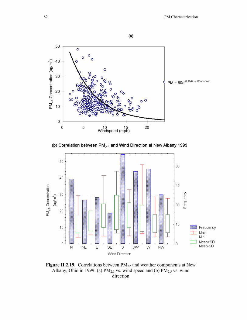
PM2.5 and Meteorological Parameters For evaluating strategies to control PM concentrations, it is important to

determine the meteorological factors that influence PM level. Correlations between PM2.5 and weather components, such as temperature, wind speed, wind direction, and relative humidity, at New Albany, Koebel, and Athens are plotted in Figures II.2.19 through Figure II.2.24. The correlation plot between PM2.5 and wind speed shows that PM concentrations decrease with increasing wind speed and vice versa. At the suburban site the PM2.5 concentration was highest when the winds were blowing from the southeast despite the low frequency of occurrence of this particular wind direction. A similar pattern was observed at the urban site in Columbus. The rural site exhibits a different pattern in that the PM2.5 concentration was highest when the winds were blowing from the south and the southeast directions.

Temperature, another important meteorological parameter, significantly affects the PM2.5 concentration and this fact is shown in the correlation plot between PM2.5 and temperature. Although temperature is related to PM2.5 at New Albany and Koebel, correlation was weak at the Athens. High PM2.5 concentration levels were generally observed when wind speed was lower than 8 mph and temperature was higher than 70°F. No significant relation was found between PM2.5 and relative humidity.


(a)

PM = 60e-0.1644 * Windspeed

0

10

20

30

40

50

0 5 10 15 20Windspeed (mph)

PM2.

5 Con

cent

ratio

n (u

g/m

3 )

Figure II.2.19. Correlations between PM2.5 and weather components at New Albany, Ohio in 1999: (a) PM2.5 vs. wind speed and (b) PM2.5 vs. wind

direction


(c)

PM = e0.0427 * Temperature

0

10

20

30

40

50

0 10 20 30 40 50 60 70 80 90Temperature (F)

PM2.

5 Con

cent

ratio

n (u

g/m

3 )

(d)

PM = -0.1055 * R.H. + 22.025R2 = 0.0216

0

10

20

30

40

50

60

40 50 60 70 80 90 100Relative Humidity

PM2.

5 Con

cent

ratio

n (u

g/m3 )

Figure II.2.20. Correlations between PM2.5 and weather components at New

Albany, Ohio in 1999: (c) PM2.5 vs. temperature and (d) PM2.5 vs. relative humidity


(a)

PM = 70e-0.1557 * Windspeed

0

10

20

30

40

50

60

70

80

0 4 8 12 16 20Windspeed (mph)

PM2.

5 Con

cent

ratio

n (u

g/m

3 )

Figure II.2.21. Correlations between PM2.5 and weather components

at Koebel, Columbus, Ohio in 1999: (a) PM2.5 vs. wind speed and (b) PM2.5 vs. wind direction


(c)


0

10

20

30

40

50

60

70

80

0 10 20 30 40 50 60 70 80 90Temperature (F)

PM2.

5 Con

cent

ratio

n (u

g/m

3 )

(d)

PM = -0.2394 * R.H. + 35.996R2 = 0.0533

0

10

20

30

40

50

60

70

80

40 50 60 70 80 90 100

Relative Humidity

PM2.

5 Con

cent

ratio

n (u

g/m

3 )

Figure II.2.22. Correlations between PM2.5 and weather components at Koebel, Columbus, Ohio in 1999: (c) PM2.5 vs. temperature and (d) PM2.5 vs.

relative humidity


(a)

PM2.5 = 60e-0.1509*wind speed

0

10

20

30

40

0 4 8 12 16 20 24Windspeed (mph)

PM2.

5 Con

cent

ratio

n (u

g/m

3 )

Figure II.2.23. Correlations between PM2.5 and weather components at Athens in 1999: (a) PM2.5 vs. wind speed and (b) PM2.5 vs. wind direction


(c)


0

10

20

30

40

20 40 60 80 100Temperature (F)

PM2.

5 Con

cent

ratio

n (u

g/m3 )

(d)

PM = 0.0559 * R.H. + 11.421R2 = 0.0052

0

10

20

30

40

40 50 60 70 80 90 100Relative Humidity

PM2.

5 Con

cent

ratio

n (u

g/m

3 )

Figure II.2.24. Correlations between PM2.5 and weather components

at Athens in 1999: (c) PM2.5 vs. temperature and (d) PM2.5 vs. relative humidity


LONG-RANGE TRANSPORT ON FINE PM2.5 DISTRIBUTION IN CENTRAL OHIO

Air quality problems related to fine particulate matter (PM2.5) in Ohio is associated with both local emission sources and pollutants transported from great distances. Industrial and urban activities in Ohio contribute to the local and regional air pollution problems. Most of the major industrial sources of fine particulate matter are located along the Ohio River valley. Significant PM sources in the neighboring states surrounding Ohio also contribute to the air quality problems in the state. Favorable meteorological situations have a major impact on the formation and transport of PM2.5 from within and outside of Ohio. A detailed understanding of the sources of pollutants and meteorological conditions affecting air quality is therefore required for any meaningful air quality planning in Ohio. The characteristics of fine particulate matter distribution are evaluated for the three monitoring sites. Particular emphasis is placed on the study of long-range transport characteristics of PM2.5 and its precursors into the central Ohio region.

The meteorological dynamics that cause air to rise or fall, and that determine its path can affect air quality by carrying air pollutants many miles from their sources.16 Therefore, the trajectory analysis technique is useful to study the movement of air parcels carrying pollutants from sources situated long distances. Cluster analysis, another technique used in this study is a multivariate statistical approach. Recent studies have used cluster analysis for various purposes. Dorling et al. applied cluster analysis of trajectories to find out the relationships between large-scale surface pressure patterns and the pollution climatology of a site.17 Also, they used cluster analysis as a tool for examining the influence of synoptic weather patterns on air and precipitation chemistry.18 Brankov et al. examined the relationship between synoptic-scale atmospheric transport patterns and concentration levels of several toxic trace elements with cluster analysis.19 Another study by Rao et al. addressed the influence of a finite number of synoptic patterns associated with pollutant transport from a different source region.20

This section presents the results of detailed analyses of the air quality issues pertaining to fine particulate matter affecting the urban, suburban and rural areas in Ohio from data monitored by the School of Health Sciences at Ohio University during 1999-2000.

Trajectory and Cluster Analysis

Trajectories are used to aid in complex decisions regarding atmospheric transport pathways.21 This study applied the hybrid single-particle lagrangian integrated trajectory (HYSPLIT4) model from National Oceanic and Atmospheric Administration (NOAA)’s Air Resource Laboratory (ARL) to


estimate backward trajectories.22 The HYSPLIT4 model is used for atmospheric emergencies, diagnostic case studies, or climatological analyses. It should be noted that the accuracy of upper air data acquired from the HYSPLIT4 model is not ideal because of the lack of extensive upper air monitoring sites in Ohio. However, if a large amount of trajectories are averaged, the errors are decreased. For this study, 24-hour back trajectories at 500 meter, which is generally in the middle of the mixed layer, on high PM days with values over 30 µg/m3 were computed. This study adapted a start time of 16 UTC, same as noon in local time, corresponding to high PM values.

Cluster analysis of backward trajectories allows for the identification of the regional source of pollutants. This analysis consists of splitting a data set into several dominant groups that are homogeneous and peculiarly different from each other as possible. In this study, the clustering approach proposed by Dorling et al.23 was chosen and modified. For each one-day (24-hour) back trajectory 6 four-hourly x-y coordinates, which are end points of the trajectory location at every four-hour interval, are used as input variables for the clustering algorithm. The original clustering algorithm generated a large number of clusters specified as the seed trajectories and assigned each of the three-day real trajectories to the seed that is closest in terms of the distance between their corresponding six-hourly coordinates. Then the seed or average trajectory of each cluster is recalculated with each real trajectory and the number of clusters is reduced by the same process that merges the two clusters whose average trajectories are closest.24 This algorithm, however, was modified in this study. Each trajectory was assigned to several clusters in terms of directions of original source regions that are x-y coordinates of starting points of 24-hour back trajectory. Main clusters in this study were divided into eight directional components, which were North, Northwest, West, Southwest, South, Southeast, East, and Northeast. In addition, an additional cluster category called “Close” was added to highlight trajectories from close proximities. The transport path was calculated by averaging trajectories assigned to each cluster. Mercator projection was selected as a plotting projection of each cluster because this study treated a small region and this projection was more convenient to plot clusters than polar stereographic projection.

Back trajectories can show the impact of upstream emissions and integrate different information including winds in the upstream layer over time, moving distances, and source location. For the study period between 1999 and 2000, 24-hour back trajectories at 500 meters for high PM days with values over 30 µg/m3 were applied using the HYSPLIT4 model from NOAA’s Air Resource Laboratory (ARL) and are presented in Figures II.2.25 a-c. The three plots of these trajectories show that the air parcel came from all around Ohio during high PM days with very few trajectories from the east. These back trajectories for the high PM days reveal that major air parcels came from the west to south direction during the study period.


Meteorological analysis can be performed using local surface wind and computed back trajectories for each area. For a detailed analysis of the PM 2.5 distribution, the path of the air parcel causing the high concentration is more important than the hourly local surface wind directions that do not account for the effect of long-range movement in the upper atmosphere. Back trajectories can show the impact of upstream emissions and integrate different information including winds in the upstream layer over time, moving distances, and source location.

Cluster analysis is an advanced method from trajectory analysis as it segregates and merges each trajectory based on its direction and/or similarity. It is a useful method to trace the original regional source of the pollutant. The clusters, their percentiles, their frequencies, and their average concentrations for the three monitoring sites during 1999-2000 are presented in Figures II.2.26 through II.2.28.

At New Albany the highest frequency of high PM days, was associated with the southwest cluster. Also the second and third highest frequencies of high PM days were observed in the south cluster and the southeast cluster passing over the Ohio River valley. The highest average PM concentration was noted along the west cluster. For Koebel the highest frequency of high PM days occurred with the southwest cluster. Other frequent high PM days were associated with clusters from the north, northwest, and south. The highest average PM concentration occurred with the north cluster, which also had the second highest frequency of high PM days. For Athens, high PM days occurred more frequently when the trajectories were from the southwest. The highest average PM concentration appeared along the west cluster.

In summary these results reveal that high PM days occurred most often along the southwest cluster, but the highest average PM concentrations appeared along the west or north clusters. Most clusters’ source regions correspond with major cities in neighboring states and major cities in Ohio. This suggests that local industrial complexes and adjoining urban areas affect PM levels in most cities in Ohio. Also, since a large amount of clusters pass over the Ohio River valley, the analysis indicate that the Ohio River valley acts as one of the main source regions of PM precursors in Ohio.


(a) New Albany, 1999-2000

35

40

45

50

-95 -90 -85 -80 -75

Cluster from WCluster from SWCluster from SCluster from SECluster from E

(b) Koebel, 1999-2000

35

40

45

50

-95 -90 -85 -80 -75

Cluster from NCluster from NWCluster from WCluster from SWCluster from SCluster from SECluster from E

Figure II.2.25. Back trajectories for high PM days at the monitoring sites selected in Ohio, 1999-2000: (a) New Albany and (b) Koebel


Figure II.2.25 (contd). Back trajectories for high PM days at the monitoring

sites selected in Ohio, 1999-2000: (c) Athens

© Athens, 1999-2000

35

40

45

50

-95 -90 -85 -80 -75

Cluster from NCluster from NWCluster from WCluster from SWCluster from SECluster from ECluster from NE


(a) New Albany, 1999-2000

35

40

45

50

-95 -90 -85 -80 -75

Cluster from WCluster from SWCluster from SCluster from SECluster from E

E (10.5%)

SE (15.8%)

S (26.3%)

SW (42.1%)

W (5.3%)

(b) New Albany, 1999-2000

0

2

4

6

8

10

W SW S SE EDirection

Freq

uenc

y

30

32

34

36

38

PM2.

5 Con

cent

ratio

n(u

g/m

3 )

Frequency Average PM2.5 Concentration

Figure II.2.26. (a) Cluster plot at New Albany, 1999-2000 (b) Frequencies and

average PM2.5 concentrations by cluster at New Albany, 1999-2000


(a) Koebel, 1999-2000

35

40

45

50

-95 -90 -85 -80 -75

Cluster from NCluster from NWCluster from WCluster from SWCluster from SCluster from SECluster from EE (3.6%)

SE (3.6%)

S (17.9%)

SW (32.1%)

W (10.7%)

NW (14.3%)N (17.9%)

(b) Koebel, 1999-2000

0

2

4

6

8

10

N NW W SW S SE EDirection

Freq

uenc

y

40

50

60

70

80

PM2.

5 Con

cent

ratio

n(u

g/m

3 )


Figure II.2.27. (a) Cluster plot at Koebel, 1999-2000 (b) Frequencies and

average PM2.5 concentrations by cluster at Koebel, 1999-2000


(a) Athens, 1999-2000

35

40

45

50

-95 -90 -85 -80 -75

Cluster from NCluster from NWCluster from WCluster from SWCluster from SECluster from ECluster from NE

NE (7.4%)

E (3.7%)

SE (3.7%)

SW (40.7%)

W (29.6%)

NW (11.1%) N (3.7%)

(b) Athens, 1999-2000

0

2

4

6

8

10

12

N NW W SW SE E NE

Direction

Freq

uenc

y

30

32

34

36

PM2.

5 Con

cent

ratio

n

(ug/

m3 )


Figure II.2.28. (a) Cluster plot at Athens, 1999-2000 (b) Frequencies and average PM2.5 concentrations by cluster at Athens, 1999-2000


RELATIONSHIP BETWEEN PM2.5 AND OZONE

The correlation between PM2.5 and ozone at New Albany and Koebel is plotted in Figure II.2.29. Data for ozone concentrations was obtained from the Ohio EPA monitoring site located at Maple Canyon, Columbus OH. This plot between PM2.5 and ozone concentration shows no significant relation between them.


(a)

PM = 0.0537 * O3 + 13.957R2 = 0.0558

0

40

80

120

160

200

240

0 40 80 120 160 200 240Ozone Concentration (ug/m3)

PM2.

5 Con

cent

ratio

n (u

g/m

3 )

(b)

PM = 0.026 * O3 + 21.761R2 = 0.0055

0

40

80

120

160

200

240

0 40 80 120 160 200 240

Ozone Concentration (ug/m3)

PM2.

5 Con

cent

ratio

n (u

g/m

3 )

Figure II.2.29. Correlations between PM2.5 and ozone in 1999: (a) New

Albany and (b) Koebel


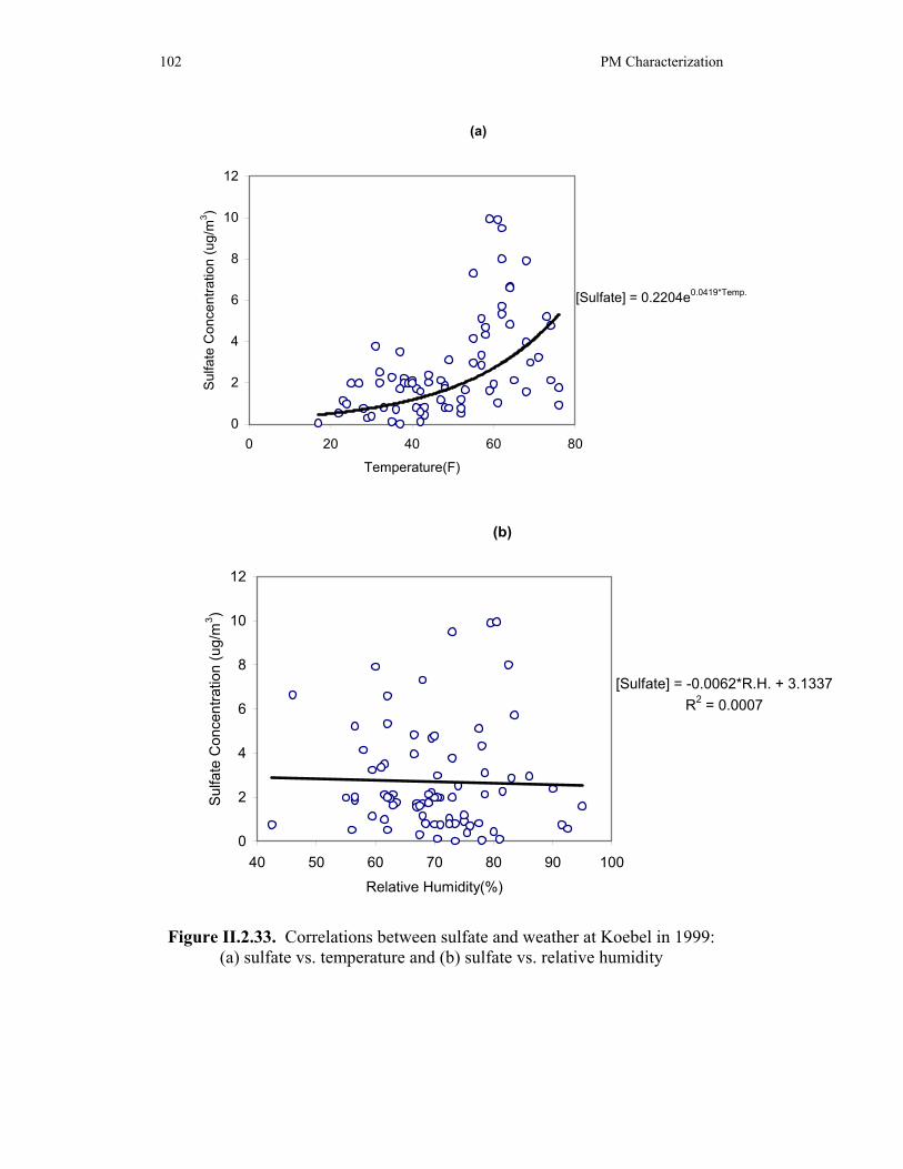
EFFECT OF WEATHER ON SULFATE AND SULFUR

Sulfate is formed from an atmospheric reaction of SO2 and can be transported far from the sources of the SO2. To evaluate strategies to control sulfate concentrations, it is important to determine the meteorological factors that influence sulfate levels. Correlations between sulfate and weather components, such as temperature, wind speed, wind direction, and relative humidity at New Albany, Koebel, and Athens are plotted in Figures II.2.30 to II.2.34 for the period from February 1999 to December 1999.

Correlation plots between sulfate and wind speed show that sulfate

concentrations decrease with increasing wind speed suggesting significant influence of wind speed on sulfate concentrations. Correlation of wind direction with sulfate reveals that the sulfate concentrations at all three sites were highest when the winds were blowing from the southeast. This indicates that there are sources of SO2 southeast of all the three sites.

Temperature, one of the important meteorological parameters, significantly

affects the sulfate concentration and this is emphasized in the correlation plot between sulfate and temperature. This correlation pattern is noted at all the three sites. High sulfate concentration levels were generally observed when the wind speed was lower than 8 mph and temperature was higher than 70°F. No significant relation could be found between sulfate and relative humidity.


(a)

[Sulfate] = 4.231e-0.1446*windspeed

0

1

2

3

4

5

6

0 5 10 15 20 25

Windspeed (mph)

Sulfa

te C

once

ntra

tion

(ug/

m3 )

Figure II.2.30. Correlations between sulfate and weather at New Albany in 1999: (a) sulfate vs. wind speed and (b) sulfate vs. wind direction


(a)

[SO4-2] = 0.1348e0.0369*Temp.

0

1

2

3

4

5

6

0 20 40 60 80Temperature(F)

Sulfa

te C

once

ntra

tion

(ug/

m3 )

(b)

[Sulfate] = 0.0207*R.H.

0

1

2

3

4

5

6

40 50 60 70 80 90 100Relative Humidity(%)

Sulfa

te C

once

ntra

tion

(ug/

m3 )

Figure II.2.31. Correlations between Sulfate and weather at New Albany in 1999: (a) sulfate vs. temperature and (b) sulfate vs. relative humidity


(a)

[Sulfate] = 6.342e-0.1489*Windspeed

0

2

4

6

8

10

12

0 5 10 15 20 25Windspeed(mph)

Sulfa

te C

once

ntra

tion

(ug/

m3 )

Figure II.2.32. Correlations between sulfate and weather at Koebel in 1999:

(a) sulfate vs. wind speed and (b) sulfate vs. wind direction


(a)

[Sulfate] = 0.2204e0.0419*Temp.

0

2

4

6

8

10

12

0 20 40 60 80

Temperature(F)

Sulfa

te C

once

ntra

tion

(ug/

m3 )

(b)

[Sulfate] = -0.0062*R.H. + 3.1337R2 = 0.0007

0

2

4

6

8

10

12

40 50 60 70 80 90 100Relative Humidity(%)

Sulfa

te C

once

ntra

tion

(ug/

m3 )

Figure II.2.33. Correlations between sulfate and weather at Koebel in 1999:

(a) sulfate vs. temperature and (b) sulfate vs. relative humidity


(a)

[Sulfate] = 9.626e-0.1829*Windspeed

0

2

4

6

8

10

0 5 10 15 20 25 30

Wind Speed (mph)

Sulfa

te C

once

ntra

tion(

ug/m

3 )

Figure II.2.34. Correlations between sulfate and weather at Athens in 1999-

2000: (a) sulfate vs. wind speed and (b) sulfate vs. wind direction


(a)

[Sulfate]= 0.024e0.0592*windspeed

0

2

4

6

8

10

0 20 40 60 80 100

Temperature(F)

Sulfa

te C

once

ntra

tion

(ug/

m3 )

(b)

[SO4-2] = 0.0059*R.H. + 1.7862

R2 = 0.0041

0

2

4

6

8

10

40 50 60 70 80 90 100

Relative Humidity(%)

Sulfa

te C

once

ntra

tion

(ug/

m3 )

Figure II.2.35. Correlations between sulfate and weather at Athens in 1999:

(c) sulfate vs. temperature and (d) sulfate vs. relative humidity


INDOOR ANALYSIS

The results of indoor analysis are assembled and presented here in the same order as the ambient outdoor results. The data tables provide PM2.5 mass and chemical composition measurements. The results are validated and spatial variations of the PM2.5 concentrations and temporal variations of PM2.5 sulfate concentrations are discussed.

PM2.5 Mass and Chemical Composition Data Summary

Tables II.2.8 to II.2.10 depict the PM2.5 mass and chemical composition data summary for the three indoor sites from February 1999 to August 2000. The average PM2.5 concentrations considered here are the arithmetic averages of the filter mass collected at each site during the period of study.

Similar to the results of ambient outdoor analysis, sulfate ion was found to be the greatest component present in the indoor filter samples. The average sulfate concentrations were highest at Koebel and lowest at New Albany. Other important components present in the samples were silicon, chlorine ion, and sodium ion. The concentrations of these components varied from site to site. Compared to concentrations at outdoor sites, very low or no concentrations of phosphates were found.


Table II.2.4. Statistical summary of PM2.5 mass and its chemical compositions at Athens (February 1999-August 2000)





NH4+ 0.7834 0.6504 0.6793 0.0024 3.8057 K+ 0.1302 0.1181 0.0940 0.0040 0.5535

Mg+2 0.1551 0.2601 0.0450 0.0101 1.0034 Ca+2 0.3068 0.4422 0.0633 0.0007 2.9486

F- 0.1836 0.1111 0.1318 0.0138 0.3867 Cl- 0.4237 0.7091 0.1689 0.0118 3.5760

NO3- 0.4594 0.6223 0.1599 0.0249 2.8292 PO4

-3 - - - - - SO4

-2 2.3260 2.1373 1.5875 0.0761 11.1147 Sum of Species 6.8907 7.9695 4.0141 0.1768 49.3184

Unidentified 9.2942 4.7509 7.7098 0.8287 17.0025


Table II.2.5. Statistical summary of PM2.5 mass and its chemical compositions at New Albany (February 1999-August 2000)





NH4+ 0.7067 0.5624 0.7085 0.0002 2.7191 K+ 0.3594 0.7186 0.1107 0.0018 4.5500

Mg+2 0.0471 0.0310 0.0355 0.0077 0.1554 Ca+2 0.3655 0.5549 0.0880 0.0009 2.8095

F- 0.1245 0.0737 0.1103 0.0176 0.3042 Cl- 0.2522 0.4167 0.1251 0.0005 4.3577

NO3- 0.4817 0.5089 0.2553 0.0242 4.2353 PO4

-3 - - - - - SO4

-2 1.9735 2.5875 1.1675 0.0649 16.5942 Sum of Species 5.8844 7.6984 3.3687 0.1280 49.8513

Unidentified 11.4110 6.5307 8.3718 0.1120 19.6551


Table II.2.6. Statistical summary of PM2.5 mass and its chemical compositions at Koebel (February 1999-August 2000)





NH4+ 0.6819 0.5772 0.6878 0.0008 2.7389 K+ 0.4823 1.2061 0.1018 0.0002 7.1066

Mg+2 0.0890 0.1603 0.0271 0.0055 1.0088 Ca+2 0.3701 0.5113 0.1403 0.0049 4.2503

F- 0.3094 0.5963 0.2431 0.1183 4.6465 Cl- 0.5002 1.0616 0.1372 0.0267 6.5299

NO3- 0.7232 0.6995 0.3732 0.0282 3.9965 PO4

-3 0.3235 - 0.3235 0.3235 0.3235 SO4

-2 2.3522 3.1596 1.3140 0.0418 24.5160 Sum of Species 7.7258 11.0526 4.1715 0.5797 78.4355

Unidentified 7.8318 2.0887 6.6805 0.4726 -10.0267


Data Validation

Similar to the outdoor data validation, the indoor data validation was conducted for (1) sum of chemical species versus PM2.5 mass concentrations, and (2) sulfate versus total sulfur, and (3) anion and cation balance.

Sum of Chemical Species Versus PM2.5 Mass Concentrations

Measured and monitored mass data were compared by plotting the scatter graphs for the sum of species against mass concentrations shown in Figures II.2.36 to II.2.38. The relationship between these two parameters was examined by plotting the mass concentration (independent variable X) against the sum of species (dependent Y).

Many of the species remain unidentified in the chemical analysis; hence, the sum of the species should always be less than or equal to the gravimetrically measured mass.25 In order to avoid double count, total sulfur (S), soluble potassium (K+) and chloride (Cl-) were excluded from the sum of species.

Figure II.2.36. Scatter plot of sum of species versus mass concentrations at Athens indoor samples (May-August 2000)

y = 0.4145x + 0.7956R = 0.80

0

2

4

6

8

10

12

14

0 5 10 15 20 25

PM2.5 Mass (ug/m3)

Sum

of S

peci

es (u

g/m

3 )


Figure II.2.37. Scatter plot of sum of species versus mass concentrations at

New Albany indoor samples for May to August 2000

Figure II.2.38. Scatter plot of sum of species versus mass

concentrations at Koebel indoor samples for May to August 2000

y = 0.4523x + 0.22R = 0.85

0

5

10

15

20

25

30

0 10 20 30 40 50

PM2.5 Mass (ug/m3)

Sum

of S

peci

es (u

g/m

3 )

y = 0.447x + 0.1808R = 0.79

0

5

10

15

20

25

0 10 20 30 40 50

PM2.5 Mass (ug/m3)

Sum

of S

peci

es (u

g/m

3 )


As the previous figures show, there is a relationship between the measured mass concentration and the sum of chemically analyzed species. Also, it is clear that the sum of species is always less than the gravimetrically measured PM2.5 mass concentrations.

Sulfate versus Total Sulfur

Sulfate (SO4-2) ion concentration was obtained by ion chromatography (IC)

analysis and the total sulfur (S) concentration was obtained from x-ray fluorescence (XRF) analysis on Teflon-membrane filters. Figures II.2.39 to II.2.41 are scatter plots of sulfate versus sulfur of the PM2.5 measurements.


-2) versus total sulfur (S) for Athens indoor samples (May to August 2000)

y = 2.6479xR = 0.68

0246

8101214

0 1 2 3 4 5PM2.5 Sulfur (ug/m3)

PM2.

5 Sul

fate

(ug/

m3 )


Figure II.2.40. Scatter plot of sulfate (SO4-2) versus total sulfur (S) for New

Albany indoor samples (May to August 2000)


-2) versus total sulfur (S) for Koebel indoor samples (May to August 2000)

y = 1.4062x + 0.7266R = 0.82

0

2

4

6

8

10

12

14

0 2 4 6 8PM2.5 Sulfur (ug/m3)

PM2.

5 Sul

fate

(ug/

m3 )

y = 1.713x + 0.5228R = 0.88

02468

10121416

0 2 4 6 8 10


PM2.

5 Sul

fate

(ug/

m3 )


A strong correlation (R = 0.68, 0.82, 0.88 for Athens, New Albany and Koebel respectively) were found for these measurements, which indicates that the majority of the PM2.5 sulfur was present as sulfate.26

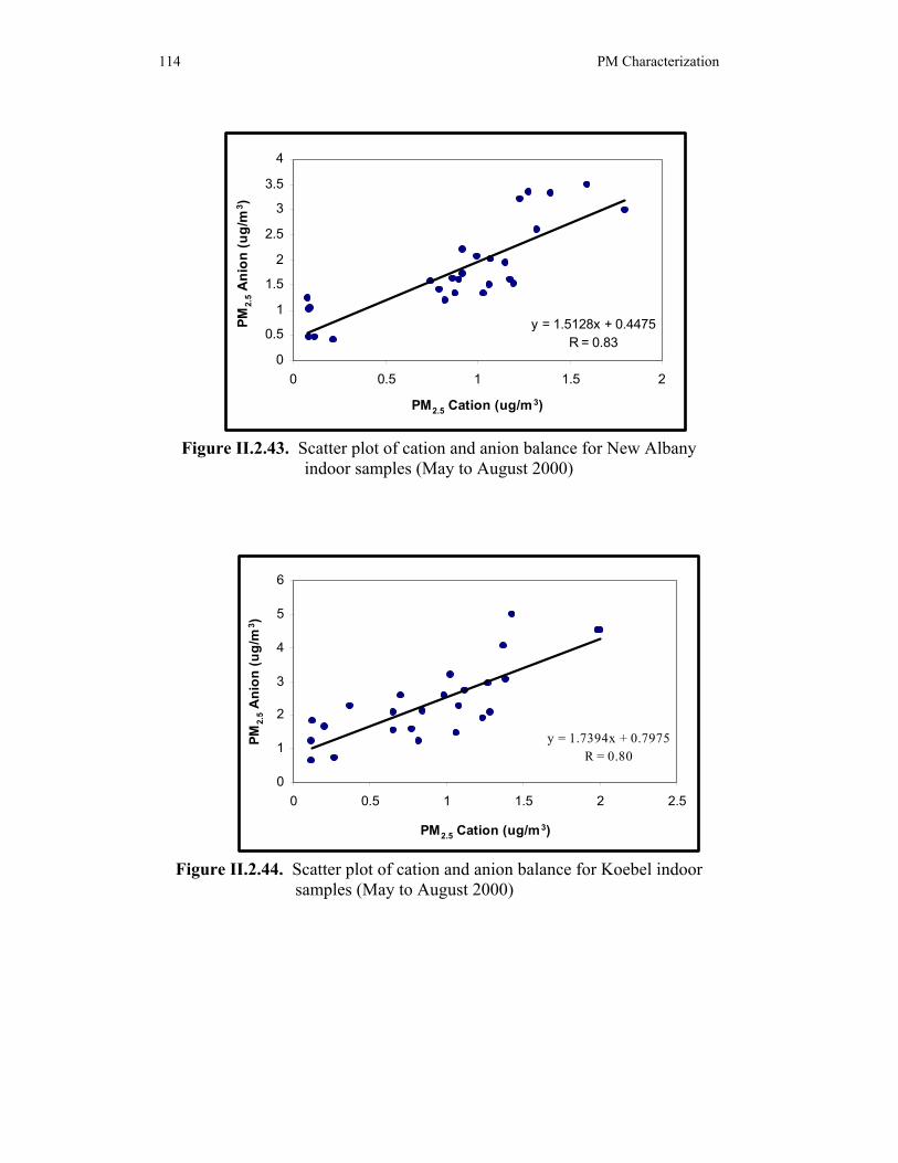
Anion and Cation balance

Ion chromatography was used to determine the concentrations of various ions present in the filter samples. Samples were analyzed for cations, lithium, sodium, ammonium, potassium, magnesium and calcium and anions, fluoride, chloride, nitrate, phosphate and sulfate. The anion and cation concentration of the PM2.5 indoor samples were obtained and correlated.

The regression plots used for anion and cation balance, shown below in

Figures II.2.42 to II.2.44, clearly show that these ionic measurements are highly correlated, with the regression coefficients of 0.69, 0.83, 0.80 for Athens, New Albany and Koebel indoor sites, respectively.

Figure II.2.42. Scatter plot of cation and anion balance for Athens indoor samples (May to August 2000)

y = 1.2548x + 1.0063R = 0.69

0

1

2

3

4

5

6

0 0.5 1 1.5 2 2.5 3 3.5


PM 2.

5 Ani

on (u

g/m

3 )


Figure II.2.43. Scatter plot of cation and anion balance for New Albany indoor samples (May to August 2000)

Figure II.2.44. Scatter plot of cation and anion balance for Koebel indoor samples (May to August 2000)

y = 1.5128x + 0.4475R = 0.83

0

0.5

1

1.5

2

2.5

3

3.5

4

0 0.5 1 1.5 2


PM2.

5 Ani

on (u

g/m

3 )

y = 1.7394x + 0.7975R = 0.80

0

1

2

3

4

5

6

0 0.5 1 1.5 2 2.5


PM2.

5 Ani

on (u

g/m

3 )


Results and Discussion

PM2.5 Chemical Species Concentration

The indoor filter samples collected from February 1999–August 2000 at the three monitoring sites in Ohio were analyzed with the ion chromatography and X-ray fluorescence techniques. Daily values of each of the components were obtained at all the sites. The results were statistically analyzed using Statistica software and box plots were obtained. The box plots show the median value along with the minimum and maximum concentrations for each of the components (Figures II.2.45 to II.2.247).

Concentrations of Cl-, NO3

-, SO4-2, PO4

-3, Li+, Na+, NH4+, K+, Mg+2,

Ca+2, Si, P, S, Cl, K, Ca, Ti, V, Cr, Co, Ni, Mn, Fe, Cu, Zn, As, Cd and Sn are shown in Figure II.2.45. They were determined for each site and then compared. The results show that sulfates are the major component present in all of the PM2.5 samples. Other abundant components included nitrate ion, ammonium ion, and silicon. High concentrations of silica were found in the indoor samples compared to the outdoor samples. Significant levels of sodium, chloride and potassium were found in the rural (Athens) samples as compared to the urban (Koebel) samples. The concentrations of each of these components varied from site to site during the period of February 1999 to August 2000.

The anion and cation average concentrations generally followed the pattern

SO4-2 >NO3 > Cl- and Na+ > NH4

+ > Ca+2 > K+ > Mg+2. Heavy metals such as titanium, vanadium, manganese, iron, copper, and zinc were found in all the samples, and iron was the most abundant species.



indoor samples at Athens for February 1999 to August 2000

Figure II.2.46. Concentrations of the chemical components present in

the indoor samples at New Albany for February 1999 to August 2000


Figure II.2.47. Concentrations of the chemical components present in the indoor samples at Koebel for February 1999 to August 2000

Major Chemical Components of PM 2.5

Similar to the previous discussion about major components of outdoor PM2.5 samples, the figures below show various chemical components of collected particulates for each site and are calculated using following equations. 1. Unidentified = measured mass – sum of 2,3,4,5,6 and 7 2. Soil = 1.62(Ca) + 2.42(Fe) + 1.94 (Ti) + 2.49 (Si) 3. Ammonium Sulfate = 1.37 (soluble sulfate) 4. Nitrate = 1.29 (soluble nitrate) 5. Phosphates = Phosphates 6. Salt = 1.65 (Cl), XRF 7. Trace elements = sum of XRF measured species – (Si + Ca + Fe + S + Cl +

Ti )

It was assumed that all particulate sulfur is ammonium sulfate. Ammonium nitrate is the main form of secondary nitrates.


Figures II.2.48 to II.2.50 show that the soil concentration at all indoor sites was higher than the outdoor soil concentrations. The soil percentage ranged from 6 percent to 10 percent at the Koebel and the Athens indoor site, respectively. Sulfate concentration was highest at Koebel and ranged from 16 percent to 21 percent of the total particulate matter mass. There was little or no phosphate found at the indoor sites. Organic matter and elemental carbon were not analyzed as a part of this study.

Figure II.2.48. Indoor PM2.5 chemical composition for Athens during February 1999 – August 2000

65.82%

0.44%

0.00%

0.56% 9.75%3.66%

19.76%



Figure II.2.49. Indoor PM2.5 chemical composition for New Albany (February 1999–August 2000)

Figure II.2.50. Indoor PM2.5 chemical composition for Koebel (February

1999–August 2000)

73.34%

0.35%0.00%

0.43%

6.60%

3.59%

15.69%


63.67%

0.43%

2.08%

1.01% 6.03%

6.00%

20.79%



Monthly Variations in Sulfate Concentration

The values of sulfate and ammonium ion found from the analyzed samples give an insight into acidity of the fine particulate fraction. Investigators have generally assumed that sulfate is present in tropospheric aerosol particles as ammonium salts and sulfuric acid.27 Figures II.2.51 to II.2.53 show the monthly sulfate ion variations for indoor sites during the period of study.

The figures show that the sulfate concentrations increased from the winter to summer at Athens. Koebel and New Albany also followed the same trend. Sulfate concentrations in general were higher in summer 1999 than the summer 2000. Indoor sites in general show a decrease in sulfate concentrations during period between months of October to March and high concentrations in summer. The average PM2.5 sulfate concentration for Athens, Koebel and New Albany for the period of study were 2.32, 1.97, 2.35 µg/m3, respectively. The average sulfate concentrations were highest at Koebel followed by Athens and with the lowest at New Albany.

The concentrations of water-soluble ions could be lower at Texas A&M University- Kingsville than the actual concentrations at the monitoring stations in Ohio due to the volatilization of the nitrates and sulfates from the Teflon filters.

Figure II.2.51. Temporal variations in indoor sulfate concentrations for Athens samples from February 1999 to August 2000


Figure II.2.52. Temporal variations in indoor sulfate concentrations for New

Albany samples from February 1999 to August 2000

Figure II.2.53. Temporal variations in indoor sulfate concentrations for

Koebel samples from February 1999 to August 2000


COMPARISON OF INDOOR AND OUTDOOR ANALYSIS

The results of the PM2.5 monitoring and the outdoor and indoor analysis for each of the chemical components were statistically analyzed and the average, standard deviation, minimum and maximum values were determined using the Statistica software.

The box-whisker distribution of concentration for the parameters,

ammonium, sulfate and nitrate for the entire period of study is shown in II.2.54 to II.2.56, respectively.

Figure II.2.54 shows the plot for ammonium ion concentration at the three sites in Ohio during the entire period of study. Ammonium ions are generally present in nature in the compound form as ammonium nitrate, ammonium chloride, and ammonium sulfate. The Athens indoor and the New Albany outdoor sites showed the highest average concentrations of ammonium ions during the period of this study.

Box-whisker plots for the anions as NO3- and SO4

-2 are shown in Figures II.2.55 and II.2.56. Figure II.2.55 represents nitrate ion distribution where the overall average concentration at the Athens outdoor and the Koebel indoor site was the highest. The main sources for increased levels of nitrate ion in the ambient air are from combustion sources. Figure II.2.57 shows sulfate ion variation among all the sites during the period of study. The average concentration was highest at the Athens indoor site and the average sulfate concentration for outdoor air was almost equal at all the three sites. The sources of sulfate ion concentration in PM2.5 are mainly from SO2 emissions from coal-fired plants, vehicular emissions and other combustion sources.


Figure II.2.54. Ammonium ion distribution in Ohio (Feb. 1999 – Aug. 2000)

Figure II.2.55. Sulfate ion distribution in Ohio (Feb. 1999 – Aug. 2000)

∗ EO = Athens Outdoor; NO = New Albany Outdoor; KO = Koebel Outdoor; EI = Athens Indoor; NI = New Albany Indoor; and KI = Koebel Indoor.


Figure II.2.56. Nitrate ion distribution in Ohio (Feb. 1999 – Aug. 2000) SUMMARY

The monitoring of fine particulate matter was carried out at three elementary schools (Koebel, New Albany and Athens) typifying an urban, suburban and rural location in Ohio from February 1999 through August 2000. Indoor and outdoor air samples were collected at each site.

On an average, 35 percent of the total particulate (PM2.5) mass was

successfully analyzed at the indoor and outdoor sites. The components determined by the chemical analysis included: F-, Cl-, NO3

-, SO4-2, PO4

-3, Li+, Na+, NH4

+, K+, Mg+2, Ca+2, Si, P, S, Cl, K, Ca, Ti, Co, Ni, V, Cr, Mn, Fe, Cu, Zn, As and Cd. The greatest percentage in the samples was sulfate. Other abundant components included phosphate, nitrate, ammonium, chloride, sodium, calcium, silicon, and iron. Soil concentrations at the indoor sites were found to be higher compared to the outdoor sites soil concentrations. The soil percentage ranged from 7 percent to 10 percent at the New Albany and the Athens indoor site respectively.

Correlation analysis between PM2.5 and weather components showed

that the PM2.5 concentrations tended to increase with rising temperatures, and decreased with increasing wind speeds. In general, PM2.5 concentration was


highest when the winds were blowing from the south and the southeast direction at all three three sites. ____________________________ NOTES

1. Spurny, K. R. 2000 and D. Hochrainer, eds. 2000. Aerosol Chemical Processes in the Environment. Boca Raton, FL: Lewis Publishers.

2. Painuly P. 2001. An Evaluation of Fine Particulate Matter in Ohio: Chemical and Transport Characteristics, Master’s thesis, Texas A&M University-Kingsville; Arya, S.P. 1999. Air Pollution Meteorology and Dispersión. New York: Oxford University Press.

3. Alvarado M. 2000. Chemical Characterization of Fine Particulate Matter in Ohio, Master’s thesis, Texas A&M University-Kingsville.

4. Kevex Instruments, Inc, 1999. Kevex 771-EDX Spectrometer User’s Guide and Tutorial.

5. Dionex Corp., 1996. Introduction to the Dionex DX 500 Chromatography Systems. 6. Tropp, R.J., S.D. Kohl, J.C. Chow, and C.A. Frazier. 1998. Final Report for the Texas

PM2.5 Sampling and Analysis Study. DRI Document No. 6570-685-7770.1F. Prepared for the City of Houston, Bureau of Air Quality Control, Houston, TX, by Desert Research Institute, Reno, NV, and TRC Environmental Corp., Chapel Hill, NC. December 15, 1998.

7. Ibid 8. Ibid 9. Ibid 10. Statistica Software, Version 5.1, StatSoft, 2300 East 144 Street, Tulsa, OK 74104 11. Malm, W. C., M. L. Pitchford, M. Scruggs, J. F. Sisler, R. Ames, S. Copeland, K. A.

Gebhart, and D. E. Day. 2000. Spatial and Seasonal patterns and temporal varabilty of haze and it’s constituents in United States: Report III. Fort Collins, CO: Cooperative Institute for Research in the Atmosphere.

12. Ibid 13. Tropp et al., Final Report. 14. Painuly, An Evaluation of Fine Particulate Matter; Hays, S.M., R. V.Gobbell, and N.

R. Ganick. 1995. Indoor Air Quality. New York: McGraw-Hill; Air & Waste Management Association. 2002. Indoor Air—A Fact Sheet for Homeowners. [cited 5 November 2002]. Available from World Wide Web: <www.awma.org/resources/education/indoorair.htm >; Plog, B.A., J. Niland, and P. J. Quinlan. 1999. Fundamentals of Industrial Hygiene. Chicago, IL: National Safety Council; Environmental Protection Agency. 1997. Revised Particulate Matter Standards. [cited 5 November 2002]. Available from World Wide Web: <http://www.epa.gov/ttn/caaa/t1/fact_sheets/pmfact.pdf >; Iiabaca, M., I. Oleata, E. Campos, J. Villaire, M. Tellez-Rojo, and I. Romieu.1999. Association between Levels of Fine Particulate and Emergency Visits for Pneumonia and other Respiratory Illnesses among Children in Santiago, Chile. J. Air & Waste Manage. Assoc. 49: 154-163; National Energy Technology Laboratory: U.S. Department of Energy. 2001. Ambient Monitoring Upper Ohio River Valley Project. [cited 5 November 2002]. Available from World Wide Web: <www.netl. doe.gov/coalpower/environment/air_q/index.html>.

15. Alavarado, Chemical Characterization of Fine Particulate Matter. 16. TNRCC Web Page. [cited 5 November 2002]. Available from World Wide Web:

http://www.tnrcc.state.tx.us/updated/air/monops/data/trajectories/maintraj.html /maintraj.html.


17. Dorling, S.R., T.D. Davies, and C.E. Pierce. 1992. Cluster analysis: a technique for estimating the synoptic meteorological controls on air and precipitation chemistry. Atmospheric Environment. 26A(14): 2583-2602.

18. Ibid. 19. Brankov, E., S.T. Rao, and P.S. Porter, P.S. 1999. Identifying pollution source regions

using multiply censored data. Environmental Science and Technology. 33(13): 2273-2277. 20 Rao, S.T., E.B. Brankov, and P.S. Porter. 1998. A trajectory-clustering-correlation

methodology for examining the long-range transport of air pollutants. Atmospheric Environment. 32(9), 1525-1534.

21. Draxler, R. R. 1996. Trajectory Optimization for Balloon Flight Planning. Weather and Forecasting. 11: 111-114.

22. Draxler, R.R. and G.D. Hess. 1997. Description of the HYSPLIT4 Modeling System. [cited 5 November 2002]. Available from World Wide Web: <http://www.arl.noaa.gov/data/ models/hysplit4/win95/arl-224.pdf>.

23. Dorling et al., Cluster analysis. 24. Dorling et al., Cluster analysis; Rao et al., A trajectory-clustering-correlation

methodology . 25. Tropp et al., Final Report. 26. Ibid. 27. Ibid.

section 2 chapter 2 - ohio epaepa.ohio.gov/portals/27/atu/section2chapter2.pdf · section 2,...

Documents