second-order differential equations ... the basic ideas of differential equations were explained in...

1110

The basic ideas of differential equations were explained in Chapter 9; there we concen-

trated on first-order equations. In this chapter we study second-order linear differential

equations and learn how they can be applied to solve problems concerning the vibrations

of springs and the analysis of electric circuits. We will also see how infinite series can be

used to solve differential equations.

Most of the solutions of the differential equation resemble sine functions when is negative but they all look like exponential functions when is large.x

x

y � � 4y � e3x

SECOND-ORDER DIFFERENTIAL EQUATIONS

17

x

y

SECOND-ORDER LINEAR EQUATIONS

A second-order linear differential equation has the form

where , , , and are continuous functions. We saw in Section 9.1 that equations ofthis type arise in the study of the motion of a spring. In Section 17.3 we will further pur-sue this application as well as the application to electric circuits.

In this section we study the case where , for all , in Equation 1. Such equa-tions are called homogeneous linear equations. Thus the form of a second-order linear homo-geneous differential equation is

If for some , Equation 1 is nonhomogeneous and is discussed in Section 17.2.Two basic facts enable us to solve homogeneous linear equations. The first of these says

that if we know two solutions and of such an equation, then the linear combinationis also a solution.

THEOREM If and are both solutions of the linear homogeneousequation (2) and and are any constants, then the function

is also a solution of Equation 2.

PROOF Since and are solutions of Equation 2, we have

and

Therefore, using the basic rules for differentiation, we have

Thus is a solution of Equation 2. My � c1y1 � c2y2

� c1�0� � c2�0� � 0

� c1�P�x�y1� � Q�x�y1� � R�x�y1� � c2 �P�x�y2� � Q�x�y2� � R�x�y2�

� P�x��c1y1� � c2y2�� Q�x��c1y1� � c2y2�� R�x��c1y1 � c2y2�

� P�x��c1y1 � c2y2�� Q�x��c1y1 � c2y2�� R�x��c1y1 � c2y2�

P�x�y� � Q�x�y� � R�x�y

P�x�y2� � Q�x�y2� � R�x�y2 � 0

P�x�y1� � Q�x�y1� � R�x�y1 � 0

y2y1

y�x� � c1y1�x� � c2y2�x�

c2c1

y2�x�y1�x�3

y � c1y1 � c2y2

y2y1

xG�x� � 0

P�x� d 2y

dx 2 � Q�x� dy

dx� R�x�y � 02

xG�x� � 0

GRQP

P�x� d 2y

dx 2 � Q�x� dy

dx� R�x�y � G�x�1

17.1

1111

The other fact we need is given by the following theorem, which is proved in moreadvanced courses. It says that the general solution is a linear combination of two linearlyindependent solutions and This means that neither nor is a constant multipleof the other. For instance, the functions and are linearly dependent,but and are linearly independent.

THEOREM If and are linearly independent solutions of Equation 2, andis never 0, then the general solution is given by

where and are arbitrary constants.

Theorem 4 is very useful because it says that if we know two particular linearly inde-pendent solutions, then we know every solution.

In general, it is not easy to discover particular solutions to a second-order linear equa-tion. But it is always possible to do so if the coefficient functions , , and are constantfunctions, that is, if the differential equation has the form

where , , and are constants and .It’s not hard to think of some likely candidates for particular solutions of Equation 5 if

we state the equation verbally. We are looking for a function such that a constant timesits second derivative plus another constant times plus a third constant times is equalto 0. We know that the exponential function (where is a constant) has the prop-erty that its derivative is a constant multiple of itself: . Furthermore, .If we substitute these expressions into Equation 5, we see that is a solution if

or

But is never 0. Thus is a solution of Equation 5 if is a root of the equation

Equation 6 is called the auxiliary equation (or characteristic equation) of the differen-tial equation . Notice that it is an algebraic equation that is obtainedfrom the differential equation by replacing by , by , and by .

Sometimes the roots and of the auxiliary equation can be found by factoring. Inother cases they are found by using the quadratic formula:

We distinguish three cases according to the sign of the discriminant .b 2 � 4ac

r2 ��b � sb 2 � 4ac

2ar1 �

�b � sb 2 � 4ac

2a7

r2r1

1yry�r 2y�ay� � by� � cy � 0

ar 2 � br � c � 06

ry � erxe rx

�ar 2 � br � c�erx � 0

ar 2erx � brerx � cerx � 0

y � erxy� � r 2erxy� � re rx

ry � erxyy�y�

y

a � 0cba

ay� � by� � cy � 05

RQP

c2c1

y�x� � c1y1�x� � c2y2�x�

P�x�y2y14

t�x� � xexf �x� � ext�x� � 5x 2f �x� � x 2

y2y1y2.y1

1112 | | | | CHAPTER 17 SECOND-ORDER DIFFERENTIAL EQUATIONS

N CASE IIn this case the roots and of the auxiliary equation are real and distinct, so and are two linearly independent solutions of Equation 5. (Note that is not aconstant multiple of .) Therefore, by Theorem 4, we have the following fact.

If the roots and of the auxiliary equation are real andunequal, then the general solution of is

EXAMPLE 1 Solve the equation .

SOLUTION The auxiliary equation is

whose roots are , . Therefore, by (8), the general solution of the given differen-tial equation is

We could verify that this is indeed a solution by differentiating and substituting into thedifferential equation. M

EXAMPLE 2 Solve .

SOLUTION To solve the auxiliary equation , we use the quadratic formula:

Since the roots are real and distinct, the general solution is

M

N CASE IIIn this case ; that is, the roots of the auxiliary equation are real and equal. Let’sdenote by the common value of and Then, from Equations 7, we have

We know that is one solution of Equation 5. We now verify that is alsoa solution:

� 0�erx � � 0�xerx� � 0

� �2ar � b�erx � �ar 2 � br � c�xerx

ay2� � by2� � cy2 � a�2re rx � r 2xerx� � b�erx � rxe rx � � cxerx

y2 � xerxy1 � erx

2ar � b � 0sor � �b

2a9

r2.r1rr1 � r2

b 2 � 4ac � 0

y � c1e (�1�s13 )x�6 � c2e (�1�s13 )x�6

r ��1 � s13

6

3r 2 � r � 1 � 0

3 d 2y

dx 2 �dy

dx� y � 0

y � c1e 2x � c2e�3x

�3r � 2

r 2 � r � 6 � �r � 2��r � 3� � 0

y� � y� � 6y � 0

y � c1er1x � c2er2 x

ay� � by� � cy � 0ar 2 � br � c � 0r2r18

er1xe r2 xy2 � er2 x

y1 � er1xr2r1

b2 � 4ac � 0

SECTION 17.1 SECOND-ORDER LINEAR EQUATIONS | | | | 1113

8

_5

_1 1

5f+gf+5g

f g

f-gg-f

f+g

FIGURE 1

N In Figure 1 the graphs of the basic solutionsand of the differential

equation in Example 1 are shown in blue andred, respectively. Some of the other solutions, linear combinations of and , are shown in black.

tf

t�x� � e�3xf �x� � e 2x

The first term is 0 by Equations 9; the second term is 0 because is a root of the auxiliaryequation. Since and are linearly independent solutions, Theorem 4 pro-vides us with the general solution.

If the auxiliary equation has only one real root , then thegeneral solution of is


SOLUTION The auxiliary equation can be factored as

so the only root is . By (10), the general solution is

M

N CASE IIIIn this case the roots and of the auxiliary equation are complex numbers. (See Appen-dix H for information about complex numbers.) We can write

where and are real numbers. [In fact, , .] Then,using Euler’s equation

from Appendix H, we write the solution of the differential equation as

where , . This gives all solutions (real or complex) of the dif-ferential equation. The solutions are real when the constants and are real. We summa-rize the discussion as follows.

If the roots of the auxiliary equation are the complex num-bers , , then the general solution of is

y � e � x�c1 cos x � c2 sin x�

ay� � by� � cy � 0r2 � � � ir1 � � � iar 2 � br � c � 011

c2c1

c2 � i�C1 � C2�c1 � C1 � C2

� e � x�c1 cos x � c2 sin x�

� e � x��C1 � C2 � cos x � i�C1 � C2 � sin x�

� C1e � x�cos x � i sin x� � C2e � x�cos x � i sin x�

y � C1er1x � C2er2 x � C1e ��i�x � C2e ��i�x

e i � cos � i sin

� s4ac � b 2 ��2a�� b��2a��

r2 � � � ir1 � � � i

r2r1

b 2 � 4ac � 0

y � c1e�3x�2 � c2 xe�3x�2

r � �32

�2r � 3�2 � 0

4r 2 � 12r � 9 � 0

4y� � 12y� � 9y � 0V

y � c1erx � c2 xerx

ay� � by� � cy � 0rar 2 � br � c � 010

y2 � xerxy1 � erxr


N Figure 2 shows the basic solutionsand in

Example 3 and some other members of the family of solutions. Notice that all of themapproach 0 as .x l �

t�x� � xe�3x�2f �x� � e�3x�2

FIGURE 2

8

_5

_2 2

5f+gf+5g

f

g

f-g

g-ff+g


SOLUTION The auxiliary equation is . By the quadratic formula, the rootsare

By (11), the general solution of the differential equation is

M

INITIAL-VALUE AND BOUNDARY-VALUE PROBLEMS

An initial-value problem for the second-order Equation 1 or 2 consists of finding a solu-tion of the differential equation that also satisfies initial conditions of the form

where and are given constants. If , , , and are continuous on an interval andthere, then a theorem found in more advanced books guarantees the existence

and uniqueness of a solution to this initial-value problem. Examples 5 and 6 illustrate thetechnique for solving such a problem.

EXAMPLE 5 Solve the initial-value problem

SOLUTION From Example 1 we know that the general solution of the differential equa-tion is

Differentiating this solution, we get

To satisfy the initial conditions we require that

From (13), we have and so (12) gives

Thus the required solution of the initial-value problem is

M

EXAMPLE 6 Solve the initial-value problem

SOLUTION The auxiliary equation is , or , whose roots are . Thus, , and since , the general solution is

Since y��x� � �c1 sin x � c2 cos x

y�x� � c1 cos x � c2 sin x

e 0x � 1 � 1� � 0�ir 2 � �1r 2 � 1 � 0

y��0� � 3y�0� � 2y� � y � 0

y � 35 e 2x �

25 e�3x

c2 � 25 c1 � 3

5c1 �23 c1 � 1

c2 � 23 c1

y��0� � 2c1 � 3c2 � 013

y�0� � c1 � c2 � 112

y��x� � 2c1e 2x � 3c2e�3x

y�x� � c1e 2x � c2e�3x

y��0� � 0y�0� � 1y� � y� � 6y � 0

P�x� � 0GRQPy1y0

y��x0 � � y1y�x0 � � y0

y

y � e 3x�c1 cos 2x � c2 sin 2x�

r �6 � s36 � 52

2�

6 � s�16

2� 3 � 2i

r 2 � 6r � 13 � 0

y� � 6y� � 13y � 0V

SECTION 17.1 SECOND-ORDER LINEAR EQUATIONS | | | | 1115

N Figure 3 shows the graphs of the solu-tions in Example 4, and

, together with some linearcombinations. All solutions approach 0 as .x l ��

t�x� � e 3x sin 2xf �x� � e 3x cos 2x

FIGURE 3

3

_3

_3 2

f

g

f-g

f+g

N Figure 4 shows the graph of the solution of theinitial-value problem in Example 5. Compare withFigure 1.

FIGURE 4

20

0_2 2

the initial conditions become

Therefore the solution of the initial-value problem is

M

A boundary-value problem for Equation 1 or 2 consists of finding a solution of thedifferential equation that also satisfies boundary conditions of the form

In contrast with the situation for initial-value problems, a boundary-value problem doesnot always have a solution. The method is illustrated in Example 7.

EXAMPLE 7 Solve the boundary-value problem

SOLUTION The auxiliary equation is

whose only root is . Therefore the general solution is

The boundary conditions are satisfied if

The first condition gives , so the second condition becomes

Solving this equation for by first multiplying through by , we get

so

Thus the solution of the boundary-value problem is

M

SUMMARY: SOLUTIONS OF ay�� by�� c 0

y � e�x � �3e � 1�xe�x

c2 � 3e � 11 � c2 � 3e

ec2

e�1 � c2e�1 � 3

c1 � 1

y�1� � c1e�1 � c2e�1 � 3

y�0� � c1 � 1

y�x� � c1e�x � c2 xe�x

r � �1

�r � 1�2 � 0orr 2 � 2r � 1 � 0

y�1� � 3y�0� � 1y� � 2y� � y � 0

V

y�x1 � � y1y�x0 � � y0

y

y�x� � 2 cos x � 3 sin x

y��0� � c2 � 3y�0� � c1 � 2


Roots of General solution

y � e� x�c1 cos x � c2 sin x�r1, r2 complex: � � i

y � c1erx � c2 xerxr1 � r2 � r

y � c1er1x � c2er2 xr1, r2 real and distinct

ar 2 � br � c � 0

N The solution to Example 6 is graphed in Figure 5. It appears to be a shifted sine curveand, indeed, you can verify that another way ofwriting the solution is

where tan � � 23y � s13 sin�x � ��

FIGURE 5

5

_5

_2π 2π

N Figure 6 shows the graph of the solution of the boundary-value problem in Example 7.

FIGURE 6

5

_5

_1 5

SECTION 17.2 NONHOMOGENEOUS LINEAR EQUATIONS | | | | 1117

19. , ,

20. , ,

, ,

22. , ,

, ,

24. , ,

25–32 Solve the boundary-value problem, if possible.

25. , ,

26. , ,

27. , ,

28. , ,

29. , ,

, ,

31. , ,

32. , ,

33. Let be a nonzero real number.(a) Show that the boundary-value problem ,

, has only the trivial solution forthe cases and .

(b) For the case , find the values of for which thisproblem has a nontrivial solution and give the corre-sponding solution.

34. If , , and are all positive constants and is a solution of the differential equation , show that

.lim x l � y�x� � 0ay� � by� � cy � 0

y�x�cba

�� 0� � 0� � 0

y � 0y�L� � 0y�0� � 0y� � �y � 0

L

y�� 1y�0� � 09y� � 18y� � 10y � 0

y��2� � 1y�0� � 2y� � 4y� � 13y � 0

y�1� � 0y�0� � 1y� � 6y� � 9y � 030.

y�� 2y�0� � 1y� � 6y� � 25y � 0

y�� 5y�0� � 2y� � 100y � 0

y�3� � 0y�0� � 1y� � 3y� � 2y � 0

y�1� � 2y�0� � 1y� � 2y� � 0

y�� 4y�0� � 34y� � y � 0

y��1� � 1y�1� � 0y� � 12y� � 36y � 0

y��0� � 1y�0� � 2y� � 2y� � 2y � 023.

y�� 2y�� 0y� � 2y� � 5y � 0

y��4� � 4y��4� � �3y� � 16y � 021.

y��0� � 4y�0� � 12y� � 5y� � 3y � 0

y��0� � �1.5y�0� � 14y� � 4y� � y � 01–13 Solve the differential equation.

2.

3. 4.

5. 6.

7. 8.

10.

12.

13.

; 14–16 Graph the two basic solutions of the differential equationand several other solutions. What features do the solutions have incommon?

14.

15.

16.

17–24 Solve the initial-value problem.

, ,

18. , , y��0� � 3y�0� � 1y� � 3y � 0

y��0� � �4y�0� � 32y� � 5y� � 3y � 017.

9 d 2y

dx 2 � 6 dy

dx� y � 0

5 d 2y

dx 2 � 2 dy

dx� 3y � 0

d 2y

dx 2 � 4 dy

dx� 20y � 0

100 d 2P

dt 2 � 200 dP

dt� 101P � 0

8 d 2y

dt 2 � 12 dy

dt� 5y � 0

2 d 2y

dt 2 � 2 dy

dt� y � 011.

y� � 3y� � 0y� � 4y� � 13y � 09.

y� � 4y� � y � 0y� � 2y�

25y� � 9y � 09y� � 12y� � 4y � 0

y� � 8y� � 12y � 0y� � 16y � 0

y� � 4y� � 4y � 0y� � y� � 6y � 01.

EXERCISES17.1

NONHOMOGENEOUS LINEAR EQUATIONS

In this section we learn how to solve second-order nonhomogeneous linear differential equa-tions with constant coefficients, that is, equations of the form

where , , and are constants and is a continuous function. The related homogeneousequation

is called the complementary equation and plays an important role in the solution of theoriginal nonhomogeneous equation (1).

ay� � by� � cy � 02

Gcba

ay� � by� � cy � G�x�1

17.2

Jimmy Hasugian

Highlight

THEOREM The general solution of the nonhomogeneous differential equation(1) can be written as

where is a particular solution of Equation 1 and is the general solution of thecomplementary Equation 2.

PROOF All we have to do is verify that if is any solution of Equation 1, then is asolution of the complementary Equation 2. Indeed

M

We know from Section 17.1 how to solve the complementary equation. (Recall that thesolution is , where and are linearly independent solutions of Equa-tion 2.) Therefore Theorem 3 says that we know the general solution of the nonhomoge-neous equation as soon as we know a particular solution . There are two methods forfinding a particular solution: The method of undetermined coefficients is straightforwardbut works only for a restricted class of functions . The method of variation of parametersworks for every function but is usually more difficult to apply in practice.

THE METHOD OF UNDETERMINED COEFFICIENTS

We first illustrate the method of undetermined coefficients for the equation

where ) is a polynomial. It is reasonable to guess that there is a particular solution that is a polynomial of the same degree as because if is a polynomial, then

is also a polynomial. We therefore substitute a polynomial (of thesame degree as ) into the differential equation and determine the coefficients.


SOLUTION The auxiliary equation of is

with roots , . So the solution of the complementary equation is

Since is a polynomial of degree 2, we seek a particular solution of the form

Then and so, substituting into the given differential equation, wehave

�2A� � �2Ax � B� � 2�Ax 2 � Bx � C � � x 2

yp� � 2Ayp� � 2Ax � B

yp�x� � Ax 2 � Bx � C

G�x� � x 2

yc � c1ex � c2e�2x

�2r � 1

r 2 � r � 2 � �r � 1��r � 2� � 0

y� � y� � 2y � 0

y� � y� � 2y � x 2V

Gyp�x� �ay� � by� � cy

yGyp

G�x

ay� � by� � cy � G�x�

GG

yp

y2y1yc � c1y1 � c2y2

� t�x� � t�x� � 0

� �ay� � by� � cy� � �ayp� � byp� � cyp �

a�y � yp �� b�y � yp �� c�y � yp � � ay� � ayp� � by� � byp� � cy � cyp

y � ypy

ycyp

y�x� � yp�x� � yc�x�

3


Jimmy Hasugian

Highlight

Jimmy Hasugian

Highlight

or

Polynomials are equal when their coefficients are equal. Thus

The solution of this system of equations is

A particular solution is therefore

and, by Theorem 3, the general solution is

M

If (the right side of Equation 1) is of the form , where and are constants,then we take as a trial solution a function of the same form, , because thederivatives of are constant multiples of .

EXAMPLE 2 Solve .

SOLUTION The auxiliary equation is with roots , so the solution of the com-plementary equation is

For a particular solution we try . Then and . Substi-tuting into the differential equation, we have

so and . Thus a particular solution is

and the general solution is

M

If is either or , then, because of the rules for differentiating thesine and cosine functions, we take as a trial particular solution a function of the form

EXAMPLE 3 Solve .

SOLUTION We try a particular solution

Then yp� � �A cos x � B sin xyp� � �A sin x � B cos x

yp�x� � A cos x � B sin x

y� � y� � 2y � sin xV

yp�x� � A cos kx � B sin kx

C sin kxC cos kxG�x�

y�x� � c1 cos 2x � c2 sin 2x �113 e 3x

yp�x� � 113 e 3x

A � 11313Ae 3x � e 3x

9Ae 3x � 4�Ae 3x � � e 3x

yp� � 9Ae 3xyp� � 3Ae 3xyp�x� � Ae 3x

yc�x� � c1 cos 2x � c2 sin 2x

�2ir 2 � 4 � 0

y� � 4y � e 3x

e k xe k xyp�x� � Aek x

kCCek xG�x�

y � yc � yp � c1ex � c2e�2x �12 x 2 �

12 x �

34

yp�x� � �12 x 2 �

12 x �

34

C � �34B � �

12A � �

12

2A � B � 2C � 02A � 2B � 0�2A � 1

�2Ax 2 � �2A � 2B�x � �2A � B � 2C � � x 2


N Figure 1 shows four solutions of the differen-tial equation in Example 1 in terms of the partic-ular solution and the functions and .t�x� � e�2x

f �x� � e xyp

FIGURE 1

8

_5

_3 3yp

yp+3gyp+2f

yp+2f+3g

N Figure 2 shows solutions of the differentialequation in Example 2 in terms of and thefunctions and .Notice that all solutions approach as and all solutions (except ) resemble sine functions when is negative.x

yp

x l ��

t�x� � sin 2xf �x� � cos 2xyp

FIGURE 2

4

_2

_4 2yp

yp+g

yp+f

yp+f+g

so substitution in the differential equation gives

or

This is true if

The solution of this system is

so a particular solution is

In Example 1 we determined that the solution of the complementary equation is. Thus the general solution of the given equation is

M

If is a product of functions of the preceding types, then we take the trial solu-tion to be a product of functions of the same type. For instance, in solving the differentialequation

we would try

If is a sum of functions of these types, we use the easily verified principle of super-position, which says that if and are solutions of

respectively, then is a solution of

EXAMPLE 4 Solve .

SOLUTION The auxiliary equation is with roots , so the solution of the com-plementary equation is . For the equation we try

Then , , so substitution in the equationgives

or ��3Ax � 2A � 3B�ex � xex

�Ax � 2A � B�ex � 4�Ax � B�ex � xex

yp1� � �Ax � 2A � B�exyp1� � �Ax � A � B�ex

yp1�x� � �Ax � B�ex

y� � 4y � xexyc�x� � c1e 2x � c2e�2x�2r 2 � 4 � 0

y� � 4y � xex � cos 2xV

ay� � by� � cy � G1�x� � G2�x�

yp1� yp2

ay� � by� � cy � G2�x�ay� � by� � cy � G1�x�

yp2yp1

G�x�

yp�x� � �Ax � B� cos 3x � �Cx � D� sin 3x

y� � 2y� � 4y � x cos 3x

G�x�

y�x� � c1ex � c2e�2x �110 �cos x � 3 sin x�

yc � c1ex � c2e�2x

yp�x� � �110 cos x �

310 sin x

B � �310A � �

110

�A � 3B � 1and�3A � B � 0

��3A � B� cos x � ��A � 3B� sin x � sin x

��A cos x � B sin x� � ��A sin x � B cos x� � 2�A cos x � B sin x� � sin x


Thus and , so , , and

For the equation , we try

Substitution gives

or

Therefore , , and

By the superposition principle, the general solution is

M

Finally we note that the recommended trial solution sometimes turns out to be a solu-tion of the complementary equation and therefore can’t be a solution of the nonhomoge-neous equation. In such cases we multiply the recommended trial solution by (or by if necessary) so that no term in is a solution of the complementary equation.

EXAMPLE 5 Solve .

SOLUTION The auxiliary equation is with roots , so the solution of the com-plementary equation is

Ordinarily, we would use the trial solution

but we observe that it is a solution of the complementary equation, so instead we try

Then

Substitution in the differential equation gives

yp� � yp � �2A sin x � 2B cos x � sin x

yp��x� � �2A sin x � Ax cos x � 2B cos x � Bx sin x

yp��x� � A cos x � Ax sin x � B sin x � Bx cos x

yp�x� � Ax cos x � Bx sin x

yp�x� � A cos x � B sin x

yc�x� � c1 cos x � c2 sin x

�ir 2 � 1 � 0

y� � y � sin x

yp�x�x 2x

yp

y � yc � yp1 � yp2 � c1e 2x � c2e�2x � ( 13 x �

29 )ex �

18 cos 2x

yp2�x� � �

18 cos 2x

�8D � 0�8C � 1

�8C cos 2x � 8D sin 2x � cos 2x

�4C cos 2x � 4D sin 2x � 4�C cos 2x � D sin 2x� � cos 2x

yp2�x� � C cos 2x � D sin 2x

y� � 4y � cos 2x

yp1�x� � (� 1

3 x �29 )ex

B � �29A � �

132A � 3B � 0�3A � 1


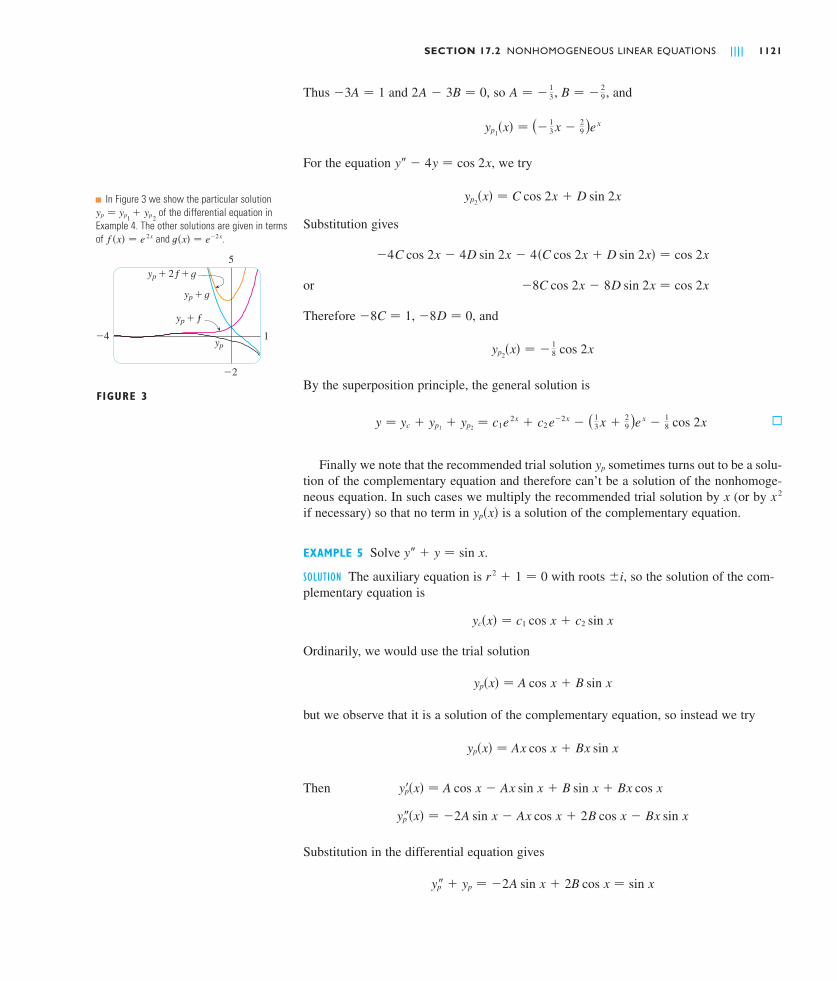
N In Figure 3 we show the particular solutionof the differential equation in

Example 4. The other solutions are given in termsof and .t�x� � e�2xf �x� � e 2x

yp � yp1� yp2

FIGURE 3

5

_2

_4 1yp

yp+g

yp+f

yp+2f+g

so , , and

The general solution is

M

We summarize the method of undetermined coefficients as follows:

SUMMARY OF THE METHOD OF UNDETERMINED COEFFICIENTS

1. If , where is a polynomial of degree , then try ,where is an th-degree polynomial (whose coefficients are determined by substituting in the differential equation).

2. If or , where is an th-degreepolynomial, then try

where and are th-degree polynomials.

Modification: If any term of is a solution of the complementary equation, multiply by (or by if necessary).

EXAMPLE 6 Determine the form of the trial solution for the differential equation.

SOLUTION Here has the form of part 2 of the summary, where , , and. So, at first glance, the form of the trial solution would be

But the auxiliary equation is , with roots , so the solutionof the complementary equation is

This means that we have to multiply the suggested trial solution by . So, instead, weuse

M

THE METHOD OF VARIATION OF PARAMETERS

Suppose we have already solved the homogeneous equation and writ-ten the solution as

where and are linearly independent solutions. Let’s replace the constants (or parame-ters) and in Equation 4 by arbitrary functions and . We look for a particu-u2�x�u1�x�c2c1

y2y1

y�x� � c1y1�x� � c2y2�x�4

ay� � by� � cy � 0

yp�x� � xe 2x�A cos 3x � B sin 3x�

x

yc�x� � e 2x�c1 cos 3x � c2 sin 3x�

r � 2 � 3ir 2 � 4r � 13 � 0

yp�x� � e 2x�A cos 3x � B sin 3x�

P�x� � 1m � 3k � 2G�x�

y� � 4y� � 13y � e 2x cos 3x

x 2xyp

yp

nRQ

yp�x� � ekxQ�x� cos mx � ekxR�x� sin mx

nPG�x� � ekxP�x� sin mxG�x� � ekxP�x� cos mx

nQ�x�yp�x� � ekxQ�x�nPG�x� � ekxP�x�

y�x� � c1 cos x � c2 sin x �12 x cos x

yp�x� � �12 x cos x

B � 0A � �12


FIGURE 4

4

_4

_2π 2π

yp

N The graphs of four solutions of the differentialequation in Example 5 are shown in Figure 4.

Jimmy Hasugian

Highlight

Jimmy Hasugian

Highlight

lar solution of the nonhomogeneous equation of the form

(This method is called variation of parameters because we have varied the parameters and to make them functions.) Differentiating Equation 5, we get

Since and are arbitrary functions, we can impose two conditions on them. One con-dition is that is a solution of the differential equation; we can choose the other conditionso as to simplify our calculations. In view of the expression in Equation 6, let’s impose thecondition that

Then

Substituting in the differential equation, we get

or

But and are solutions of the complementary equation, so

and Equation 8 simplifies to

Equations 7 and 9 form a system of two equations in the unknown functions and .After solving this system we may be able to integrate to find and and then the partic-ular solution is given by Equation 5.

EXAMPLE 7 Solve the equation , .

SOLUTION The auxiliary equation is with roots , so the solution ofis . Using variation of parameters, we seek a solution

of the form

Then

Set

u1� sin x � u2� cos x � 010

yp� � �u1� sin x � u2� cos x� � �u1 cos x � u2 sin x�

yp�x� � u1�x� sin x � u2�x� cos x

c1 sin x � c2 cos xy� � y � 0�ir 2 � 1 � 0

0 � x � ��2y� � y � tan x

u2u1

u2�u1�

a�u1�y1� � u2�y2�� G9

ay2� � by2� � cy2 � 0anday1� � by1� � cy1 � 0

y2y1

u1�ay1� � by1� � cy1� � u2�ay2� � by2� � cy2 � � a�u1�y1� � u2�y2�� G8

a�u1�y1� � u2�y2� � u1y1� � u2y2�� b�u1y1� � u2y2�� c�u1y1 � u2y2 � � G

yp� � u1�y1� � u2�y2� � u1y1� � u2y2�

u1�y1 � u2�y2 � 07

yp

u2u1

yp� � �u1�y1 � u2�y2 � � �u1y1� � u2y2��6

c2

c1

yp�x� � u1�x� y1�x� � u2�x� y2�x�5

ay� � by� � cy � G�x�


Then

For to be a solution we must have

Solving Equations 10 and 11, we get

(We seek a particular solution, so we don’t need a constant of integration here.) Then,from Equation 10, we obtain

So

(Note that for .) Therefore


My�x� � c1 sin x � c2 cos x � cos x ln�sec x � tan x�

� �cos x ln�sec x � tan x�

yp�x� � �cos x sin x � �sin x � ln�sec x � tan x�� cos x

0 � x � ��2sec x � tan x 0

u2�x� � sin x � ln�sec x � tan x�

u2� � �sin x

cos x u1� � �

sin2x

cos x�

cos2x � 1

cos x� cos x � sec x

u1�x� � �cos xu1� � sin x

u1��sin2x � cos2x� � cos x tan x

yp� � yp � u1� cos x � u2� sin x � tan x11

yp

yp� � u1� cos x � u2� sin x � u1 sin x � u2 cos x


; 11–12 Graph the particular solution and several other solutions.What characteristics do these solutions have in common?

11. 12.

13–18 Write a trial solution for the method of undeterminedcoefficients. Do not determine the coefficients.

13.

14.

15.

17.

y� � 4y � e 3x � x sin 2x18.

y� � 2y� � 10y � x 2e�x cos 3x

y� � 3y� � 4y � �x 3 � x�e x16.

y� � 9y� � 1 � xe 9x

y� � 9y� � xe�x cos �x

y� � 9y � e 2x � x 2 sin x

y� � 4y � e�xy� � 3y� � 2y � cos x

1–10 Solve the differential equation or initial-value problemusing the method of undetermined coefficients.

1.

2.

3.

4.

6.

7. , ,

8. , ,

, ,

10. , , y��0� � 0y �0� � 1y� � y� � 2y � x � sin 2x

y��0� � 1y�0� � 2y� � y� � xe x9.

y��0� � 2y�0� � 1y� � 4y � e x cos x

y��0� � 0y�0� � 2y� � y � e x � x 3

y� � 2y� � y � xe�x

y� � 4y� � 5y � e�x5.

y� � 6y� � 9y � 1 � x

y� � 2y� � sin 4x

y� � 9y � e 3x

y� � 3y� � 2y � x 2

EXERCISES17.2

FIGURE 5

π2

2.5

_1

0yp

N Figure 5 shows four solutions of the differential equation in Example 7.

SECTION 17.3 APPLICATIONS OF SECOND-ORDER DIFFERENTIAL EQUATIONS | | | | 1125

24. ,

26.

27.

28. y� � 4y� � 4y �e�2x

x 3

y� � 2y� � y �e x

1 � x 2

y� � 3y� � 2y � sin�e x �

y� � 3y� � 2y �1

1 � e�x25.

0 � x � ��2y� � y � sec3x19–22 Solve the differential equation using (a) undetermined coef-ficients and (b) variation of parameters.

19. 20.

22.

23–28 Solve the differential equation using the method ofvariation of parameters.

23. , 0 � x � ��2y� � y � sec2x

y� � y� � e x

y� � 2y� � y � e2x21.

y� � 2y� � 3y � x � 24y� � y � cos x

APPLICATIONS OF SECOND-ORDER DIFFERENTIAL EQUATIONS

Second-order linear differential equations have a variety of applications in science andengineering. In this section we explore two of them: the vibration of springs and electriccircuits.

VIBRATING SPRINGS

We consider the motion of an object with mass at the end of a spring that is either ver-tical (as in Figure 1) or horizontal on a level surface (as in Figure 2).

In Section 6.4 we discussed Hooke’s Law, which says that if the spring is stretched (orcompressed) units from its natural length, then it exerts a force that is proportional to :

where is a positive constant (called the spring constant). If we ignore any external resist-ing forces (due to air resistance or friction) then, by Newton’s Second Law (force equalsmass times acceleration), we have

This is a second-order linear differential equation. Its auxiliary equation is with roots , where . Thus the general solution is

which can also be written as

where (frequency)

(amplitude)

(See Exercise 17.) This type of motion is called simple harmonic motion.

� is the phase angle�sin � �c2

Acos �

c1

A

A � sc12 � c2

2

� � sk�m

x�t� � A cos��t � �

x�t� � c1 cos �t � c2 sin �t

� � sk�m r � ��imr 2 � k � 0

m d 2x

dt 2 � kx � 0orm d 2x

dt 2 � �kx1

k

restoring force � �kx

xx

m

17.3

FIGURE 2

FIGURE 1

x0 x

equilibrium position

m

m

x

0

x m

equilibriumposition

EXAMPLE 1 A spring with a mass of 2 kg has natural length m. A force of Nis required to maintain it stretched to a length of m. If the spring is stretched to alength of m and then released with initial velocity 0, find the position of the mass atany time .

SOLUTION From Hooke’s Law, the force required to stretch the spring is

so . Using this value of the spring constant , together with in Equation 1, we have

As in the earlier general discussion, the solution of this equation is

We are given the initial condition that . But, from Equation 2, Therefore . Differentiating Equation 2, we get

Since the initial velocity is given as , we have and so the solution is

M

DAMPED VIBRATIONS

We next consider the motion of a spring that is subject to a frictional force (in the case ofthe horizontal spring of Figure 2) or a damping force (in the case where a vertical springmoves through a fluid as in Figure 3). An example is the damping force supplied by ashock absorber in a car or a bicycle.

We assume that the damping force is proportional to the velocity of the mass and actsin the direction opposite to the motion. (This has been confirmed, at least approximately,by some physical experiments.) Thus

where is a positive constant, called the damping constant. Thus, in this case, Newton’sSecond Law gives

or

m d 2x

dt 2 � c dx

dt� kx � 03

m d 2x

dt 2 � restoring force � damping force � �kx � c dx

dt

c

damping force � �c dx

dt

x�t� � 15 cos 8t

c2 � 0x��0� � 0

x��t� � �8c1 sin 8t � 8c2 cos 8t

c1 � 0.2x�0� � c1.x�0� � 0.2

x�t� � c1 cos 8t � c2 sin 8t2

2 d 2x

dt 2 � 128x � 0

m � 2kk � 25.6�0.2 � 128

k�0.2� � 25.6

t0.7

0.725.60.5V

1126 | | | | CHAPTER 17 SECOND-ORDER DIFFERENTIAL EQUATIONSSc

hwin

n Cy

clin

g an

d Fi

tnes

s

FIGURE 3

m

Equation 3 is a second-order linear differential equation and its auxiliary equation is. The roots are

According to Section 17.1 we need to discuss three cases.

N CASE I (overdamping)In this case and are distinct real roots and

Since , , and are all positive, we have , so the roots and given byEquations 4 must both be negative. This shows that as . Typical graphs of

as a function of are shown in Figure 4. Notice that oscillations do not occur. (It’s pos-sible for the mass to pass through the equilibrium position once, but only once.) This isbecause means that there is a strong damping force (high-viscosity oil or grease)compared with a weak spring or small mass.

N CASE II (critical damping)This case corresponds to equal roots

and the solution is given by

It is similar to Case I, and typical graphs resemble those in Figure 4 (see Exercise 12), butthe damping is just sufficient to suppress vibrations. Any decrease in the viscosity of thefluid leads to the vibrations of the following case.

N CASE III (underdamping)Here the roots are complex:

where

The solution is given by

We see that there are oscillations that are damped by the factor . Since and, we have so as . This implies that as

that is, the motion decays to 0 as time increases. A typical graph is shown in Figure 5.t l �;x l 0t l �e��c�2m�t l 0��c�2m� � 0m 0

c 0e��c�2m�t

x � e��c�2m�t�c1 cos �t � c2 sin �t�

� �s4mk � c 2

2m

r1

r2� � �

c

2m� �i

c2 � 4mk � 0

x � �c1 � c2t�e��c�2m�t

r1 � r2 � �c

2m

c2 � 4mk � 0

c 2 4mk

txt l �x l 0

r2r1sc 2 � 4mk � ckmc

x � c1er1t � c2er2t

r2r1

c2 � 4mk 0

r2 ��c � sc 2 � 4mk

2mr1 �

�c � sc 2 � 4mk

2m4

mr 2 � cr � k � 0


FIGURE 4Overdamping

x

t0

x

t0

FIGURE 5 Underdamping

x

t0

x=Ae–(c/2m)t

x=_Ae–(c/2m)t

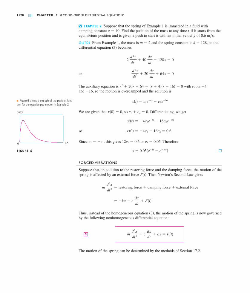
EXAMPLE 2 Suppose that the spring of Example 1 is immersed in a fluid with damping constant . Find the position of the mass at any time if it starts from theequilibrium position and is given a push to start it with an initial velocity of m�s.

SOLUTION From Example 1, the mass is and the spring constant is , so thedifferential equation (3) becomes

or

The auxiliary equation is with roots and , so the motion is overdamped and the solution is

We are given that , so . Differentiating, we get

so

Since , this gives or . Therefore

M

FORCED VIBRATIONS

Suppose that, in addition to the restoring force and the damping force, the motion of thespring is affected by an external force . Then Newton’s Second Law gives

Thus, instead of the homogeneous equation (3), the motion of the spring is now governedby the following nonhomogeneous differential equation:

The motion of the spring can be determined by the methods of Section 17.2.

m d 2x

dt 2 � c dx

dt� kx � F�t�5

� �kx � c dx

dt� F�t�

m d 2x

dt 2 � restoring force � damping force � external force

F�t�

x � 0.05�e�4t � e�16t �

c1 � 0.0512c1 � 0.6c2 � �c1

x��0� � �4c1 � 16c2 � 0.6

x��t� � �4c1e�4t � 16c2e�16t

c1 � c2 � 0x�0� � 0

x�t� � c1e�4t � c2e�16t

�16�4r 2 � 20r � 64 � �r � 4��r � 16� � 0

d 2x

dt 2 � 20 dx

dt� 64x � 0

2 d 2x

dt 2 � 40 dx

dt� 128x � 0

k � 128m � 2

0.6tc � 40

V


N Figure 6 shows the graph of the position func-tion for the overdamped motion in Example 2.

FIGURE 6

0.03

0 1.5

A commonly occurring type of external force is a periodic force function

In this case, and in the absence of a damping force ( ), you are asked in Exercise 9 touse the method of undetermined coefficients to show that

If , then the applied frequency reinforces the natural frequency and the result isvibrations of large amplitude. This is the phenomenon of resonance (see Exercise 10).

ELECTRIC CIRCUITS

In Sections 9.3 and 9.5 we were able to use first-order separable and linear equations toanalyze electric circuits that contain a resistor and inductor (see Figure 5 on page 582 orFigure 4 on page 605) or a resistor and capacitor (see Exercise 29 on page 607). Now thatwe know how to solve second-order linear equations, we are in a position to analyze thecircuit shown in Figure 7. It contains an electromotive force (supplied by a battery orgenerator), a resistor , an inductor , and a capacitor , in series. If the charge on thecapacitor at time is , then the current is the rate of change of with respect to : . As in Section 9.5, it is known from physics that the voltage drops acrossthe resistor, inductor, and capacitor are

respectively. Kirchhoff’s voltage law says that the sum of these voltage drops is equal tothe supplied voltage:

Since , this equation becomes

which is a second-order linear differential equation with constant coefficients. If the chargeand the current are known at time 0, then we have the initial conditions

and the initial-value problem can be solved by the methods of Section 17.2.

Q��0� � I�0� � I0Q�0� � Q0

I0Q0

L d 2Q

dt 2 � R dQ

dt�

1

C Q � E�t�7

I � dQ�dt

L dI

dt� RI �

Q

C� E�t�

Q

CL

dI

dtRI

I � dQ�dttQQ � Q�t�t

CLRE

�0 � �

x�t� � c1 cos �t � c2 sin �t �F0

m��2 � � 02 �

cos �0t 6

c � 0

where �0 � � � sk�m F�t� � F0 cos �0t


FIGURE 7

C

E

R

L

switch

A differential equation for the current can be obtained by differentiating Equation 7with respect to and remembering that :

EXAMPLE 3 Find the charge and current at time in the circuit of Figure 7 if, H, F, , and the initial charge and

current are both 0.

SOLUTION With the given values of , , , and , Equation 7 becomes

The auxiliary equation is with roots

so the solution of the complementary equation is

For the method of undetermined coefficients we try the particular solution

Then

Substituting into Equation 8, we have

or

Equating coefficients, we have

oror

The solution of this system is and , so a particular solution is


� e�20t�c1 cos 15t � c2 sin 15t� �4

697 �21 cos 10t � 16 sin 10t�

Q�t� � Qc�t� � Qp�t�

Qp�t� � 1697 �84 cos 10t � 64 sin 10t�

B � 64697A � 84

697

�16A � 21B � 0 �400A � 525B � 0

21A � 16B � 4 525A � 400B � 100

�525A � 400B� cos 10t � ��400A � 525B� sin 10t � 100 cos 10t

� 625�A cos 10t � B sin 10t� � 100 cos 10t

��100A cos 10t � 100B sin 10t� � 40��10A sin 10t � 10B cos 10t�

Qp��t� � �100A cos 10t � 100B sin 10t

Qp��t� � �10A sin 10t � 10B cos 10t

Qp�t� � A cos 10t � B sin 10t

Qc�t� � e�20t�c1 cos 15t � c2 sin 15t�

r ��40 � s�900

2� �20 � 15i

r 2 � 40r � 625 � 0

d 2Q

dt 2 � 40 dQ

dt� 625Q � 100 cos 10t8

E�t�CRL

E�t� � 100 cos 10tC � 16 � 10�4L � 1R � 40 �tV

L d 2I

dt 2 � R dI

dt�

1

C I � E��t�

I � dQ�dtt


Imposing the initial condition , we get

To impose the other initial condition, we first differentiate to find the current:

Thus the formula for the charge is

and the expression for the current is

M

In Example 3 the solution for consists of two parts. Since asand both and are bounded functions,

So, for large values of ,

and, for this reason, is called the steady state solution. Figure 8 shows how the graphof the steady state solution compares with the graph of in this case.

Comparing Equations 5 and 7, we see that mathematically they are identical.This suggests the analogies given in the following chart between physical situations that,at first glance, are very different.

We can also transfer other ideas from one situation to the other. For instance, the steadystate solution discussed in Note 1 makes sense in the spring system. And the phenomenonof resonance in the spring system can be usefully carried over to electric circuits as elec-trical resonance.

NOTE 2

QQp�t�

Q�t� � Qp�t� � 4697 �21 cos 10t � 16 sin 10t�

t

as t l Qc�t� � 42091 e�20t��63 cos 15t � 116 sin 15t� l 0

sin 15tcos 15tt l e�20t l 0Q�t�NOTE 1

I�t� � 12091 �e�20t��1920 cos 15t � 13,060 sin 15t� � 120��21 sin 10t � 16 cos 10t��

Q�t� �4

697 � e�20t

3 ��63 cos 15t � 116 sin 15t� � �21 cos 10t � 16 sin 10t�

c2 � �4642091 I�0� � �20c1 � 15c2 �

640697 � 0

� 40697 ��21 sin 10t � 16 cos 10t�

I �dQ

dt� e�20t ��20c1 � 15c2 � cos 15t � ��15c1 � 20c2 � sin 15t�

c1 � �84697Q�0� � c1 �

84697 � 0

Q�0� � 0


FIGURE 8

0.2

_0.2

0 1.2

Qp

Q

L d 2Q

dt 2 � R dQ

dt�

1

C Q � E�t�7

m d 2x

dt 2 � c dx

dt� kx � F�t�5

Spring system Electric circuit

x displacement Q chargevelocity current

m mass L inductancec damping constant R resistancek spring constant elastance

external force electromotive forceE�t�F�t�1�C

I � dQ�dtdx�dt


12. Consider a spring subject to a frictional or damping force.(a) In the critically damped case, the motion is given by

. Show that the graph of crosses the -axis whenever and have opposite signs.

(b) In the overdamped case, the motion is given by, where . Determine a condition

on the relative magnitudes of and under which thegraph of crosses the -axis at a positive value of .

A series circuit consists of a resistor with , aninductor with H, a capacitor with F, and a12-V battery. If the initial charge and current are both 0, findthe charge and current at time t.

14. A series circuit contains a resistor with , an induc-tor with H, a capacitor with F, and a 12-Vbattery. The initial charge is C and the initial cur-rent is 0.(a) Find the charge and current at time t.

; (b) Graph the charge and current functions.

15. The battery in Exercise 13 is replaced by a generator produc-ing a voltage of . Find the charge at time t.

16. The battery in Exercise 14 is replaced by a generator pro-ducing a voltage of .(a) Find the charge at time t.

; (b) Graph the charge function.

Verify that the solution to Equation 1 can be written in theform .

18. The figure shows a pendulum with length L and the angle from the vertical to the pendulum. It can be shown that , as afunction of time, satisfies the nonlinear differential equation

where is the acceleration due to gravity. For small values of we can use the linear approximation and then the

differential equation becomes linear.(a) Find the equation of motion of a pendulum with length

1 m if is initially 0.2 rad and the initial angular velocityis .

(b) What is the maximum angle from the vertical?(c) What is the period of the pendulum (that is, the time to

complete one back-and-forth swing)?(d) When will the pendulum first be vertical?(e) What is the angular velocity when the pendulum is

vertical?

¨L

d�dt � 1 rad�s

sin � t

d 2

dt 2 �t

L sin � 0

x�t� � A cos��t � ��17.

E�t� � 12 sin 10t

E�t� � 12 sin 10t

Q � 0.001C � 0.005L � 2

�R � 24

C � 0.002L � 1�R � 2013.

ttxc2c1

r1 r2x � c1er 1 t � c2er 2 t

c2c1txx � c1ert � c2tert

1. A spring has natural length and a mass. A force ofis needed to keep the spring stretched to a length of .

If the spring is stretched to a length of and then releasedwith velocity , find the position of the mass after seconds.

2. A spring with an mass is kept stretched beyond itsnatural length by a force of . The spring starts at its equi-librium position and is given an initial velocity of . Findthe position of the mass at any time .

A spring with a mass of 2 kg has damping constant 14, and a force of 6 N is required to keep the spring stretched mbeyond its natural length. The spring is stretched 1 m beyondits natural length and then released with zero velocity. Find theposition of the mass at any time t.

4. A force of 13 N is needed to keep a spring with a 2-kg massstretched 0.25 m beyond its natural length. The damping con-stant of the spring is .(a) If the mass starts at the equilibrium position with a

velocity of , find its position at time .

; (b) Graph the position function of the mass.

5. For the spring in Exercise 3, find the mass that would producecritical damping.

6. For the spring in Exercise 4, find the damping constant thatwould produce critical damping.

; 7. A spring has a mass of 1 kg and its spring constant is .The spring is released at a point 0.1 m above its equilibriumposition. Graph the position function for the following valuesof the damping constant c: 10, 15, 20, 25, 30. What type ofdamping occurs in each case?

; 8. A spring has a mass of 1 kg and its damping constant isThe spring starts from its equilibrium position with a

velocity of 1 m�s. Graph the position function for the follow-ing values of the spring constant k: 10, 20, 25, 30, 40. Whattype of damping occurs in each case?

Suppose a spring has mass and spring constant and let. Suppose that the damping constant is so small

that the damping force is negligible. If an external forceis applied, where , use the method

of undetermined coefficients to show that the motion of themass is described by Equation 6.

10. As in Exercise 9, consider a spring with mass , spring con-stant , and damping constant , and let . If an external force is applied (the applied frequency equals the natural frequency), use the method ofundetermined coefficients to show that the motion of the massis given by .

11. Show that if , but is a rational number, then themotion described by Equation 6 is periodic.

��0�0 � �

x�t� � c1 cos �t � c2 sin �t � �F0 ��2m��t sin �t

F�t� � F0 cos �t� � sk�m c � 0k

m

�0 � �F�t� � F0 cos �0t

� � sk�m km9.

c � 10.

k � 100

t0.5 m�s

c � 8

0.53.

t1 m�s

32 N0.4 m8-kg

t01.1 m

1 m25 N5-kg0.75 m

EXERCISES17.3

SERIES SOLUTIONS

Many differential equations can’t be solved explicitly in terms of finite combinations ofsimple familiar functions. This is true even for a simple-looking equation like

But it is important to be able to solve equations such as Equation 1 because they arise fromphysical problems and, in particular, in connection with the Schrödinger equation in quan-tum mechanics. In such a case we use the method of power series; that is, we look for asolution of the form

The method is to substitute this expression into the differential equation and determine thevalues of the coefficients This technique resembles the method of undeter-mined coefficients discussed in Section 17.2.

Before using power series to solve Equation 1, we illustrate the method on the simplerequation in Example 1. It’s true that we already know how to solve this equa-tion by the techniques of Section 17.1, but it’s easier to understand the power seriesmethod when it is applied to this simpler equation.

EXAMPLE 1 Use power series to solve the equation .

SOLUTION We assume there is a solution of the form

We can differentiate power series term by term, so

In order to compare the expressions for and more easily, we rewrite as follows:

Substituting the expressions in Equations 2 and 4 into the differential equation, weobtain

or

n�0 ��n � 2��n � 1�cn�2 � cn �xn � 05

n�0 �n � 2��n � 1�cn�2 xn �

n�0 cn xn � 0

y� �

n�0 �n � 2��n � 1�cn�2 xn4

y�y�y

y� � 2c2 � 2 � 3c3 x � � � � �

n�2 n�n � 1�cn xn�23

y� � c1 � 2c2 x � 3c3 x 2 � � � � �

n�1 ncn xn�1

y � c0 � c1 x � c2 x 2 � c3 x 3 � � � � �

n�0 cn xn2

y� � y � 0V

y� � y � 0

c0, c1, c2, . . . .

y � f �x� �

n�0 cn xn � c0 � c1 x � c2 x 2 � c3 x 3 � � � �

y� � 2xy� � y � 01

17.4

SECTION 17.4 SERIES SOLUTIONS | | | | 1133

N By writing out the first few terms of (4), youcan see that it is the same as (3). To obtain (4),we replaced by and began the sum-mation at 0 instead of 2.

n � 2n

If two power series are equal, then the corresponding coefficients must be equal. There-fore the coefficients of in Equation 5 must be 0:

Equation 6 is called a recursion relation. If and are known, this equation allows us to determine the remaining coefficients recursively by putting in succession.

By now we see the pattern:

Putting these values back into Equation 2, we write the solution as

Notice that there are two arbitrary constants, and Mc1.c0

� c0

n�0 ��1�n

x 2n

�2n�!� c1

n�0 ��1�n

x 2n�1

�2n � 1�!

� � c1�x �x 3

3!�

x 5

5!�

x 7

7!� � � � � ��1�n

x 2n�1

�2n � 1�!� � � ��

� c0�1 �x 2

2!�

x 4

4!�

x 6

6!� � � � � ��1�n

x 2n

�2n�!� � � ��

y � c0 � c1x � c2x 2 � c3x 3 � c4x 4 � c5x 5 � � � �

For the odd coefficients, c2n�1 � ��1�n c1

�2n � 1�!

For the even coefficients, c2n � ��1�n c0

�2n�!

Put n � 5: c7 � �c5

6 � 7� �

c1

5! 6 � 7� �

c1

7!

Put n � 4: c6 � �c4

5 � 6� �

c0

4! 5 � 6� �

c0

6!

Put n � 3: c5 � �c3

4 � 5�

c1

2 � 3 � 4 � 5�

c1

5!

Put n � 2: c4 � �c2

3 � 4�

c0

1 � 2 � 3 � 4�

c0

4!

Put n � 1: c3 � �c1

2 � 3

Put n � 0: c2 � �c0

1 � 2

n � 0, 1, 2, 3, . . .c1c0

n � 0, 1, 2, 3, . . .cn�2 � �cn

�n � 1��n � 2�6

�n � 2��n � 1�cn�2 � cn � 0

xn


We recognize the series obtained in Example 1 as being the Maclaurin seriesfor and . (See Equations 11.10.16 and 11.10.15.) Therefore we could write thesolution as

But we are not usually able to express power series solutions of differential equations interms of known functions.

EXAMPLE 2 Solve .

SOLUTION We assume there is a solution of the form

Then

and

as in Example 1. Substituting in the differential equation, we get

This equation is true if the coefficient of is 0:

We solve this recursion relation by putting successively in Equation 7:

Put n � 3: c5 �5

4 � 5 c3 �

1 � 5

2 � 3 � 4 � 5 c1 �

1 � 5

5! c1

Put n � 2: c4 �3

3 � 4 c2 � �

3

1 � 2 � 3 � 4 c0 � �

3

4! c0

Put n � 1: c3 �1

2 � 3 c1

Put n � 0: c2 ��1

1 � 2 c0

n � 0, 1, 2, 3, . . .

n � 0, 1, 2, 3, . . .cn�2 �2n � 1

�n � 1��n � 2� cn7

�n � 2��n � 1�cn�2 � �2n � 1�cn � 0

xn

n�0 ��n � 2��n � 1�cn�2 � �2n � 1�cn �xn � 0

n�0 �n � 2��n � 1�cn�2 xn �

n�1 2ncn xn �

n�0 cn xn � 0

n�0 �n � 2��n � 1�cn�2 xn � 2x

n�1 ncn xn�1 �

n�0 cn xn � 0

y� �

n�2 n�n � 1�cn xn�2 �

n�0 �n � 2��n � 1�cn�2 xn

y� �

n�1 ncn xn�1

y �

n�0 cn xn

y� � 2xy� � y � 0V

y�x� � c0 cos x � c1 sin x

sin xcos xNOTE 1

SECTION 17.4 SERIES SOLUTIONS | | | | 1135

n�1 2ncn x n �

n�0 2ncn x n

In general, the even coefficients are given by

and the odd coefficients are given by

The solution is

or

M

In Example 2 we had to assume that the differential equation had a series solu-tion. But now we could verify directly that the function given by Equation 8 is indeed asolution.

Unlike the situation of Example 1, the power series that arise in the solution ofExample 2 do not define elementary functions. The functions

and y2�x� � x �

n�1 1 � 5 � 9 � � � � � �4n � 3�

�2n � 1�! x 2n�1

y1�x� � 1 �1

2! x 2 �

n�2 3 � 7 � � � � � �4n � 5�

�2n�! x 2n

NOTE 3

NOTE 2

� � c1�x �

n�1 1 � 5 � 9 � � � � � �4n � 3�

�2n � 1�! x 2n�1�

y � c0�1 �1

2! x 2 �

n�2 3 � 7 � � � � � �4n � 5�

�2n�! x 2n�8

� � c1�x �1

3! x 3 �

1 � 5

5! x 5 �

1 � 5 � 9

7! x 7 �

1 � 5 � 9 � 13

9! x 9 � � � ��

� c0�1 �1

2! x 2 �

3

4! x 4 �

3 � 7

6! x 6 �

3 � 7 � 11

8! x 8 � � � ��

y � c0 � c1 x � c2 x 2 � c3 x 3 � c4 x 4 � � � �

c2n�1 �1 � 5 � 9 � � � � � �4n � 3�

�2n � 1�! c1

c2n � �3 � 7 � 11 � � � � � �4n � 5�

�2n�! c0

Put n � 7: c9 �13

8 � 9 c7 �

1 � 5 � 9 � 13

9! c1

Put n � 6: c8 �11

7 � 8 c6 � �

3 � 7 � 11

8! c0

Put n � 5: c7 �9

6 � 7 c5 �

1 � 5 � 9

5! 6 � 7 c1 �

1 � 5 � 9

7! c1

Put n � 4: c6 �7

5 � 6 c4 � �

3 � 7

4! 5 � 6 c0 � �

3 � 7

6! c0


are perfectly good functions but they can’t be expressed in terms of familiar functions. Wecan use these power series expressions for and to compute approximate values of thefunctions and even to graph them. Figure 1 shows the first few partial sums (Taylor polynomials) for , and we see how they converge to . In this way we cangraph both and in Figure 2.

If we were asked to solve the initial-value problem

we would observe from Theorem 11.10.5 that

This would simplify the calculations in Example 2, since all of the even coefficients wouldbe 0. The solution to the initial-value problem is

y�x� � x �

n�1 1 � 5 � 9 � � � � � �4n � 3�

�2n � 1�! x 2n�1

c1 � y��0� � 1c0 � y�0� � 0

y��0� � 1y�0� � 0y� � 2xy� � y � 0

NOTE 4

y2y1

y1y1�x�T0, T2, T4, . . .

y2y1

CHAPTER 17 REVIEW | | | | 1137

11. , ,

12. The solution of the initial-value problem

is called a Bessel function of order 0.(a) Solve the initial-value problem to find a power series

expansion for the Bessel function.

; (b) Graph several Taylor polynomials until you reach one thatlooks like a good approximation to the Bessel function onthe interval .��5, 5�

y��0� � 0y�0� � 1x 2 y� � xy� � x 2 y � 0

y��0� � 1y�0� � 0y� � x 2 y� � xy � 01–11 Use power series to solve the differential equation.

1. 2.

4.

5. 6.

7.

8.

, ,

10. , , y��0� � 0y�0� � 1y� � x 2 y � 0

y��0� � 0y�0� � 1y� � xy� � y � 09.

y� � xy

�x � 1�y� � y� � 0

y� � yy� � xy� � y � 0

�x � 3�y� � 2y � 0y� � x 2 y3.

y� � xyy� � y � 0

EXERCISES17.4

15

_15

_2.5 2.5

›

fi

FIGURE 1

2

_8

_2 2

T¸

T¡¸

FIGURE 2

REVIEW

C O N C E P T C H E C K

17

(b) What is the complementary equation? How does it helpsolve the original differential equation?

(c) Explain how the method of undetermined coefficientsworks.

(d) Explain how the method of variation of parameters works.

4. Discuss two applications of second-order linear differentialequations.

5. How do you use power series to solve a differential equation?

1. (a) Write the general form of a second-order homogeneous linear differential equation with constant coefficients.

(b) Write the auxiliary equation.(c) How do you use the roots of the auxiliary equation to solve

the differential equation? Write the form of the solution foreach of the three cases that can occur.

2. (a) What is an initial-value problem for a second-order differ-ential equation?

(b) What is a boundary-value problem for such an equation?

3. (a) Write the general form of a second-order nonhomogeneouslinear differential equation with constant coefficients.

Determine whether the statement is true or false. If it is true, explain why.If it is false, explain why or give an example that disproves the statement.

1. If and are solutions of , then is also a solution of the equation.

2. If and are solutions of , thenis also a solution of the equation.c1 y1 � c2 y2

y� � 6y� � 5y � xy2y1

y1 � y2y� � y � 0y2y1

3. The general solution of can be written as

4. The equation has a particular solution of the form

yp � Ae x

y� � y � e x

y � c1 cosh x � c2 sinh x

y� � y � 0

T R U E - F A L S E Q U I Z

1–10 Solve the differential equation.

1.

2.

3.

4.

5.

6.

7.

8.

9.

10. ,

11–14 Solve the initial-value problem.

11. , ,

12. , ,

13. , ,

14. , ,

15. Use power series to solve the initial-value problem

y��0� � 1y�0� � 0y� � xy� � y � 0

y��0� � 2y�0� � 19y� � y � 3x � e �x

y��0� � 1y�0� � 0y� � 5y� � 4y � 0

y��0� � 1y�0� � 2y� � 6y� � 25y � 0

y��1� � 12y�1� � 3y� � 6y� � 0

0 � x � ��2d 2y

dx 2 � y � csc x

d 2y

dx 2 �dy

dx� 6y � 1 � e�2x

d 2y

dx 2 � 4y � sin 2x

d 2y

dx 2 � 2 dy

dx� y � x cos x

d 2y

dx 2 �dy

dx� 2y � x 2

d 2y

dx 2 � 4 dy

dx� 5y � e 2x

4y� � 4y� � y � 0

y� � 3y � 0

y� � 4y� � 13y � 0

y� � 2y� � 15y � 0

16. Use power series to solve the equation

17. A series circuit contains a resistor with , an inductorwith H, a capacitor with F, and a 12-V bat-tery. The initial charge is C and the initial current is 0. Find the charge at time t.

18. A spring with a mass of 2 kg has damping constant 16, and aforce of N keeps the spring stretched m beyond its natural length. Find the position of the mass at time if it starts at the equilibrium position with a velocity of m�s.

19. Assume that the earth is a solid sphere of uniform density withmass and radius mi. For a particle of mass within the earth at a distance from the earth’s center, thegravitational force attracting the particle to the center is

where is the gravitational constant and is the mass of theearth within the sphere of radius .

(a) Show that .

(b) Suppose a hole is drilled through the earth along a diame-ter. Show that if a particle of mass is dropped from restat the surface, into the hole, then the distance ofthe particle from the center of the earth at time is given by

where .(c) Conclude from part (b) that the particle undergoes simple

harmonic motion. Find the period T.(d) With what speed does the particle pass through the center

of the earth?

k 2 � GM�R3 � t�R

y��t� � �k 2 y�t�

ty � y�t�

m

Fr ��GMm

R3 r

rMrG

Fr ��GMr m

r 2

rmR � 3960M

2.4t

0.212.8

Q � 0.01C � 0.0025L � 2

�R � 40

y� � xy� � 2y � 0

E X E R C I S E S


second-order differential equations ... the basic ideas of differential equations were explained in...

Documents