secaucus living shoreline project monitoring plan ... in red indicate techniques that ... rtk gps...

1

Hurricane Sandy Coastal Resiliency Competitive Grants Program #42279 DOI/NFWF Building Ecological Solutions to Coastal Community Hazards

Secaucus Living Shoreline Project Monitoring Plan

Partnership for the Delaware Estuary and Barnegat Bay Partnership

Site: NJDEP-NFWF Secaucus Tidal Stream Restoration and Enhancement

Dates Active: March 1, 2015 – March 2018

Project Lead: Brian Thumpayil, RVA Engineers

Partners: NJDEP, NWF, Barnegat Bay Partnership (BBP), Partnership for the Delaware Estuary (PDE), Township of Secaucus, Remington, Vernick and Arango Engineers

Project Design Team: Township of Secaucus, Remington, Vernick and Arango Engineers

Monitoring Plan Design Team: Barnegat Bay Partnership (BBP), Partnership for the Delaware Estuary (PDE) Point of Contact: LeeAnn Haaf (PDE), Erin Reilly (BBP), Joshua Moody (PDE), Martha Maxwell Doyle (BBP), Danielle Kreeger (PDE) Monitoring Implementation Team: LeeAnn Haaf lead, Erin Reilly co-lead Project Type Description of the overall project including the type of living shoreline being installed (bio-based, hybrid, etc...) or restoration technique being employed that requires a structured monitoring program. Tidal stream restoration and enhancement Project Goal and Objectives List project goal and provide reasoning for this goal being selected (e.g.: erosion control as goal due to value of infrastructure behind shoreline or value of habitat, etc...). State project objectives as monitoring actions that will assess the ability of the project to meet its defined goal. See PDE monitoring framework for a listing and description of restoration types and goals. This project aims to protect valuable infrastructure and low lying areas from minor tidal surges and periodic flooding by enhancing drainage capacity of pre-existing tidal ditches. Objectives:

1. Monitor topography of drainage channels 2. Monitor extent of biological (vegetative) community 3. Monitor stream volume

Project Location Provide GPS coordinates of project centroid and short description of the project area/location. Provide map as Figure 1. The project is located along the Hackensack River in Secaucus, NJ in two pre-existing drainage ditches. Ditch 1, the northern ditch, is located on the northern border of the Secaucus Meadowlands Extended Stay America, and north of

2

Route 3. Ditch 2, the southern ditch, is located just south of Route 3, between a small marina owned and operated by the town of Secaucus and the Secaucus/Meadowlands Red Roof Plus. Ditch 1: Riverward Extent: 40.801, -74.065 Inland Extent: 40.800, -74.064 Ditch 2: Riverward Extent: 40.799, -74.066 Inland Extent: 40.799, -74.065 Treatment Description Description of treatment and control (if applicable) designs including: relationships to existing structures on site; replications; and components. Detail should be reflective of the current stage of project and should be updated throughout the course of the project to reflect any, and all, changes or adaptive management activities. Previous entries should not be altered, but a new section should be added by date. This section will serve as a journal of the conception and evolution of treatments/installations.

The tidal stream restoration treatments for each ditch are as follows:

Ditch 1: Ditch 1 will be dredged to a depth of -2.5' at the landward end (i.e. check valve) and a depth of -5.5' at the Hackensack River end. Three planting areas have been selected, two on the southwest side and one on the northeast side. These areas are located ~25'-70' from the landward end.

Ditch 2: Ditch 2 will be dredged to a depth of -4.2’ at the landward end (i.e. check valve) and a depth of -4.2’ at the Hackensack River end. One planting area has been selected on the northeast side located ~40'-55' from the landward end.

Both ditches will receive new check valves. See engineering specs for details.

Endpoints Description of the parametric value or temporal scale that will dictate the completion of the project according to permit(s). This project does not have specific end point goals, but aims to track the changes to the physical and biological conditions of interest as listed in the monitoring tasks until 3/2018. Monitoring Tasks Metrics of interest required by monitoring plan and associated methods used for data collection. Provide monitoring table from Monitoring Framework including reasoning for methodologies chosen. Methods in red indicate techniques that require specialized equipment, knowledge, permitting, or training. Methods in green indicate techniques that do not require and specialized, equipment, knowledge, permitting, or training besides on-site instruction for from trained staff. Photo documentation is a mandatory monitoring task at ALL visits to a project site as well as a monitoring task on all monitoring dates.

Table 1 Monitoring metric and method table

Restoration

Type and Goal

Class of

Metrics Metric Method Reasoning

Sampling

Type

(See Sampling

Design Type)

Tidal

Stream Photo Appearance

Fixed Photo

Points

Provides visual documentation

of project and site over the

course of the monitoring

Photo

3

Restorati

on and

Enhance

ment

timeline

Physical

Stream Volume

Crest-Stage

Gage/ Measure

water depth

Estimates of water volume in

channel, possibly provide info

on highest volume since last

reading

Readings

from

gage/

Stratified

Physical

Sampling

Creek/Channel

Morphometry

RTK GPS Survey

Measure changes in

morphometry of channels as a

result of changes in flow and

channel depth along cross

sections

Targeted

Point

Sampling

Position of

Contiguous

Vegetated Shoreline

(Horizontal Change)

RTK GPS Survey

Fixed Photo

Points

Measure changes in the

horizontal extent of the

vegetative community over

time as a result of the

treatment

Targeted

Point

Sampling

Biological

Vegetation:

Survivorship of

Planted Plugs

Counts Logged

on Data Sheets

Measure persistence of

planted vegetation within the

treatments

Targeted

Biological

Sample

Vegetation: Growth

Measurement

of Blade Height

with Meter Stick

Measure above ground

growth of vegetation within

the treatments

Targeted

Biological

Sample

Vegetation:

Robustness- Light

Attenuation

Measurement

with light meter

logged on data

sheet

Measure above ground

growth of vegetation to

determine canopy robustness

of vegetation within the

treatments

Targeted

Biological

Sample

Chemical Water Salinity

YSI or other

Acceptable

Equipment

Measure local conditions

within which to frame the

results of other data collected

Site Level

Sampling

Sampling Frame Description of the area within which data will be collected, referenced to existing structures, relative position within the local tidal spectrum, and three-dimensional features of interest (e.g: tops of structural components). GPS coordinates (4 minimum) demarcating the bounds of the sampling frame are to be listed. These coordinates are to be collected during the first survey (see Table 2 below). Include a map of the sampling frame as Figure 2.

4

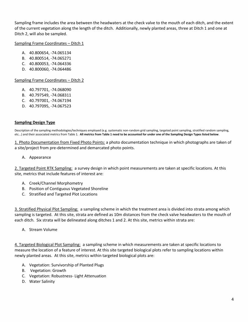
Sampling frame includes the area between the headwaters at the check valve to the mouth of each ditch, and the extent of the current vegetation along the length of the ditch. Additionally, newly planted areas, three at Ditch 1 and one at Ditch 2, will also be sampled.

Sampling Frame Coordinates – Ditch 1

A. 40.800654, -74.065134 B. 40.800514, -74.065271 C. 40.800053, -74.064336 D. 40.800060, -74.064486

Sampling Frame Coordinates – Ditch 2

A. 40.797701, -74.068090 B. 40.797549, -74.068311 C. 40.797001, -74.067194 D. 40.797095, -74.067523

Sampling Design Type

Description of the sampling methodologies/techniques employed (e.g. systematic non-random grid sampling, targeted point sampling, stratified random sampling, etc...) and their associated metrics from Table 1. All metrics from Table 1 need to be accounted for under one of the Sampling Design Types listed below.

1. Photo Documentation from Fixed Photo Points: a photo documentation technique in which photographs are taken of a site/project from pre-determined and demarcated photo points.

A. Appearance 2. Targeted Point RTK Sampling: a survey design in which point measurements are taken at specific locations. At this site, metrics that include features of interest are:

A. Creek/Channel Morphometry B. Position of Contiguous Vegetated Shoreline C. Stratified and Targeted Plot Locations

3. Stratified Physical Plot Sampling: a sampling scheme in which the treatment area is divided into strata among which sampling is targeted. At this site, strata are defined as 10m distances from the check valve headwaters to the mouth of each ditch. Six strata will be delineated along ditches 1 and 2. At this site, metrics within strata are:

A. Stream Volume

4. Targeted Biological Plot Sampling: a sampling scheme in which measurements are taken at specific locations to measure the location of a feature of interest. At this site targeted biological plots refer to sampling locations within newly planted areas. At this site, metrics within targeted biological plots are:

A. Vegetation: Survivorship of Planted Plugs B. Vegetation: Growth C. Vegetation: Robustness- Light Attenuation D. Water Salinity

5

5. Site Level Sampling (Measured or Observational): a sampling scheme in which either data will likely not vary across the AOI (e.g. water temperature, etc..) and sub-sampling is not required, or it is not advisable to limit the scope of monitoring within treatment area (e.g. stratified sampling locals) as the data of interest may be aggregated and thus not captured by targeted sampling (e.g. shellfish aggregates).

A. Water Salinity Sampling Spatial Resolution For each Sampling Design Type, describe the spatial resolution at which the methodologies will be employed, including targeted or delineated (strata) physical or zonated locals. Provide a map (Figure 3) of the spatial resolution of the data collection (e.g. quadrat location, sample well locations, grid system resolution, structural locations, etc...).

1. Photo Documentation from Fixed Photo Points: Fixed photo points will be located, at minimum, at each end of a project site. Any other angles of interest can be added to the photo documentation series. Exact locations of fixed photo points will be provided after the first visit to the site (see Table 2).

2. Targeted Point RTK Sampling: An RTK point will capture the latitude, longitude and elevation and points will be taken at 1-meter intervals along the continuous vegetation line, along each stream bed transect, and within each of the targeted biological and stratified physical sampling plots within the sampling frame.

A. Stream Bed Transects B. Contiguous Vegetation Line C. Stratified Physical/Biological Sampling Plots

3. Stratified Physical Plot Sampling: At each ditch, six transects will be placed perpendicular to the ditches, numbering 1-6 moving from the headwaters to the mouth. On each transect there will be one 1m2 sampling plot located approximately 10m apart in the ditches center. (Figure 3).

4. Targeted Biological Plot Sampling: At this site targeted biological plots refer to sampling locations within newly planted areas. Within each newly planted area, two 1m2 assessment plots will be positioned 0.5m from each river/landward extents towards the center.

Sampling Temporal Resolution Description and table of planned sampling events including large scale factor level events such as site characterization, baseline data collection, as-built surveying and annual monitoring, as well as seasonally focused monitoring such as vegetation monitoring occurring during maximum growth seasons and aerial survey during leaf-off seasons. Sample data is characterized as being collected "Before and After Installation" which refers to the dredging and installation of check valve for use in statistical analysis. As of now there is no additional annual monitoring planned for this site.

6

Table 2 Example Data collection schedule

Date Temporal Factor Level Data Collected by Collected On

April 18th,

2016

Before Installation Targeted Point Sampling PDE/BBP 5/31/2016; 6/1/2016

April 18th,

2016

Before Installation Stratified Physical Plot Sampling PDE/BBP 5/31/2016; 6/1/2016

TBD After Installation Targeted Point Sampling PDE/BBP

TBD After Installation Stratified Physical Plot Sampling PDE/BBP

TBD After Installation Targeted Biological Plot Sampling PDE/BBP

Recommended Minimum Long-Term Monitoring Description of the recommended monitoring past the duration of the stated monitoring timeline It is recommended that all metrics with associated methods that do not require and specialized, equipment, knowledge, permitting, or training besides on-site instruction for from trained staff (indicated in green in the Monitoring Tasks Table (1) above) continue to be collected annually subsequent to the end date of the project with the following exception:

● Photo Documentation from Fixed Photo Points: This metric should be collected twice annually A. Early Spring: before the plants emerge from senescence B. Late Summer: When maximum vegetative growth is visible

Statistical Methodology Description of the statistical methods that will be used to evaluate data (e.g. BACI design, 2-way ANOVA, multiple-regression, etc...) A before-after statistical analysis will be conducted as a one way ANOVA to detect changes in metrics as a result of the installation. Factor levels will be: Before Installation; and After Installation. Additionally, changes in metrics of interest will be evaluated for coincidences with changes in other metrics and correlative relationships. Sampling Methodologies

See Metrics and Methods

7

Figure 1 Location

8

Figure 2. Sampling frame for Secaucus tidal stream restoration and enhancement project

9

Figure 3 Stratified Biological Sampling Plot locations and Targeted Biological Plots

Transects Stratified Physical Plot

T 1

T 2

T 3

T 4

T 5

T 6

Targeted Biological Plot

Stratified Physical Plot

T 1

T 2

T 3

T 4

T 5

T 6

Transects Targeted Biological Plot

10

Metrics and Methods for Secaucus

Fixed Photo Points

Standard Operating Procedure No. SOP-XX Date Prepared: 8/23/16 (v2) Prepared By: __ ______________________

Description

This Standard Operating Procedure (SOP) describes the collection of fixed photo points at restoration projects. Photo

documentation of a site will be taken from predetermined and demarcated photo points to assess the changes over

time of the area. Because locational positioning of restoration structures and relevant areas of interest (e.g. current

vegetation line, location of outfalls etc.) is being measured in other ways, it is not critical that photo-point photographs

are an exact replicate of previous photos, but rather capture the entire area of interest.

Summary of Approach

Changes over time are critical to document, whether it be for a permit or educational use. By taking pictures at fixed

locations, more exact changes can be documented over time. Importantly, when taking fixed photo points, it is crucial

to find the location of the fixed position and to identify the features that you are supposed to capture in the

photograph. To ensure that this occurs, detailed descriptions of location, direction, and features should be documented

so that all photos capture the same area. In addition to fixed photo points, supplementary photographs should be taken

at the discretion of the photographers to document other interesting conditions at the site.

Equipment and Materials

Camera

Photo Journal/Station Location Guide

Topographic and/or site map with photo point locations

Extra batteries for camera (if applicable)

GPS unit (if applicable) Optional:

Aerial photos and previous photos if available • GoPro with Telescoping Pole for overhead images

Ruler (for scale on close up views of streams and vegetation)

Posts for dedicating fixed photo points if the site plan allows for installation

Procedures

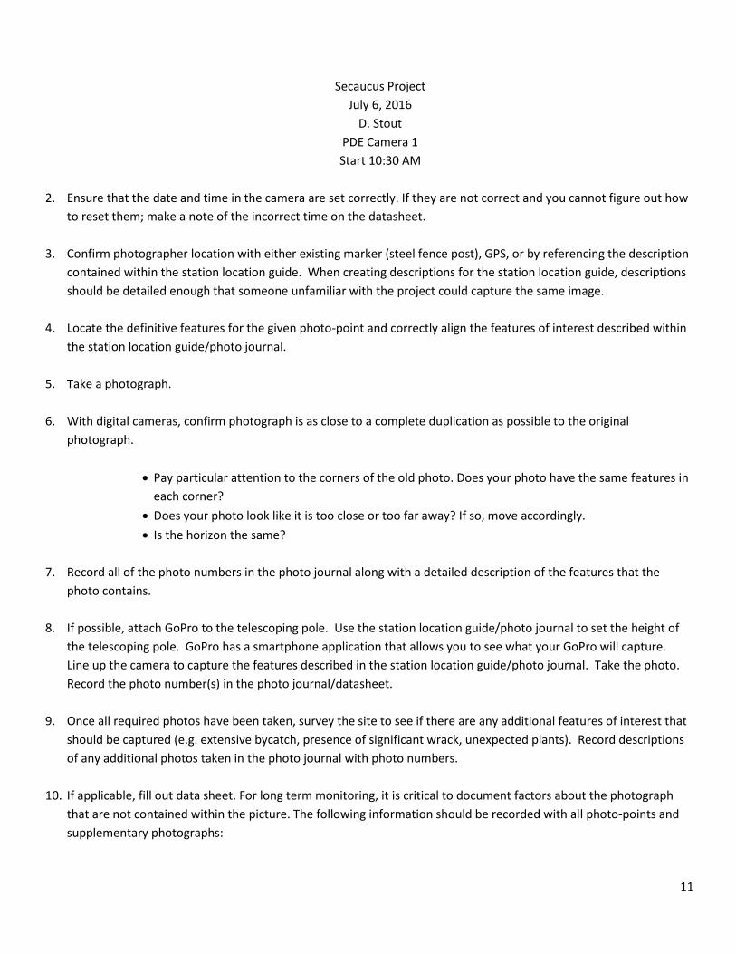
1. In the photo journal, record information about the site including site ID, date, photographer name, camera being

used and start time. An example can be seen below:

11

Secaucus Project

July 6, 2016

D. Stout

PDE Camera 1

Start 10:30 AM

2. Ensure that the date and time in the camera are set correctly. If they are not correct and you cannot figure out how

to reset them; make a note of the incorrect time on the datasheet.

3. Confirm photographer location with either existing marker (steel fence post), GPS, or by referencing the description

contained within the station location guide. When creating descriptions for the station location guide, descriptions

should be detailed enough that someone unfamiliar with the project could capture the same image.

4. Locate the definitive features for the given photo-point and correctly align the features of interest described within

the station location guide/photo journal.

5. Take a photograph.

6. With digital cameras, confirm photograph is as close to a complete duplication as possible to the original

photograph.

Pay particular attention to the corners of the old photo. Does your photo have the same features in

each corner?

Does your photo look like it is too close or too far away? If so, move accordingly.

Is the horizon the same?

7. Record all of the photo numbers in the photo journal along with a detailed description of the features that the

photo contains.

8. If possible, attach GoPro to the telescoping pole. Use the station location guide/photo journal to set the height of

the telescoping pole. GoPro has a smartphone application that allows you to see what your GoPro will capture.

Line up the camera to capture the features described in the station location guide/photo journal. Take the photo.

Record the photo number(s) in the photo journal/datasheet.

9. Once all required photos have been taken, survey the site to see if there are any additional features of interest that

should be captured (e.g. extensive bycatch, presence of significant wrack, unexpected plants). Record descriptions

of any additional photos taken in the photo journal with photo numbers.

10. If applicable, fill out data sheet. For long term monitoring, it is critical to document factors about the photograph

that are not contained within the picture. The following information should be recorded with all photo-points and

supplementary photographs:

12

Photo file name

Date the photograph was taken

Name of photographer

Location (site and stream)

Description of photograph

11. Photos are to be transferred off of the camera shortly after they are collected.

12. It is important to have file and data management of pictures. Follow appropriate project specific protocols for

archiving photos (i.e., PDE-Best Practice #2 Procedure for Archiving Photo Data)

Best Practice #14 Set-Up and Use of the Trimble RTK GPS

9/18/14 Created By: Kurt Cheng, Priscilla Cole, Jessie Buckner

Materials

Data Logger (Controller)

Antenna (Receiver)

Pole (2 sections inside case)

Mifi

Battery Pack (2) – for Antenna

Controller handle (clip) – attaches data logger to the pole

Case for mifi (waterproof)

Tape measure/Measuring stick

Charging device (1), Charging cords (2)

Pelican Hard Case

Protocols

Day Before 1. Charge three parts:

a. Battery pack(s) for Antenna - removable packs fit into charger which has cord to plug into electrical

outlet

b. Mifi – cord connects device to electrical outlet (USB)

c. Data Logger – cord connects device to electrical outlet

13

Survey Day

Assembly & Setup

1. Turn on mifi and place into waterproof case

2. Assemble the pole by screwing 2 parts together

3. Place charged battery pack into Antenna

4. Turn on Antenna

5. Screw Antenna onto top of pole

6. Measure distance from the base of antenna to the bottom of the pole (typical 1.94m)

7. Turn on Data Controller

Data Controller Settings

1. Main Menu Setup Internetwifi

2. Main MenuMeasureCreate New JobGive the job a name

3. Main MenuMeasureMeasure PointsVRS RoverVRS-CMRX

Logging Points

Point density of sampling will be determined on a site by site basis. At some sites constructed structures may be GPSed,

at others transects may run though the project area, and at others shoreline or creek morphology might be captured.

See each projects Monitoring Plan.

1. You should now be on the data capture screen

2. Insert “height to antenna” measurement in height field (#6 under assembly)

3. Naming Scheme – All points need to have a name, but the code-field is optional

a. Point names will auto-advance in sequential order (numbers or alphabetical), unless otherwise

modified.

b. Code field is just another attribute field to capture additional data. PDE staff often use the code to

capture vegetation or sediment types.

4. Press “Enter” (bottom right)

5. Press “Capture Observation” (bottom right)

Error Handling

1. Errors will occur if Mifi is moved too far away from the device.

2. Mifi can get too hot if left in its case for too long on sunny days. Keep the case cool and remove the device from

its case if needed.

3. High RMS – Points will not log if movement is too high. In this case, abandon the point and recapture.

4. Cannot connect with satellites – reconnect

Day After

Uploading Files

1. Plug RTK handset into computer using USB cord

2. Power handset ON (green button on bottom left-hand corner)

3. On your computer, when the window pops up click Connect without setting up your device

14

a. ClickFile Management

i. Browse the Contents of your Device

1. Trimble data

a. Living Shorelines

i. Export

1. Select Site Files

2. Copy (Ctrl-c)

3. Open T:\Science Stuff\GIS\Living Shorelines\SITE

Name\RTK_Data

4. Paste Site Files (Ctrl-v)

5. DO NOT DELETE FROM HANDSET

4. On the handset screen, click “X” in the top-right corner to exit

5. Hold power button down for 5 seconds and follow prompts to Shutdown

6. Return handset to library and make sure that the RTK is signed in.

7. Email Data Specialist to alert about new data creation

Best Practice # 18 Field Protocol for Vegetation: Survivorship

3/17/16

Description: Collect data at 1 m2 vegetation plots to assess vegetation survivorship of planted plugs at

restoration sites.

Materials

Required for sampling

1.0 m2 PVC quadrat

2 meter stick

GPS unit-with sites

Camera

Writing utensil

Clip board

Maps of sites in plastic sheet covers

Datasheets

Plant field guide

15

Protocols

A stratified random sampling technique to determine the location of permanent survey plots will be used. The

number of sampling plots depends on the vegetation community, final number of plantings, number and size

of planting areas and spacing of plantings. Data should be collected at 3 or more sampling plots to allow for

statistical analysis, when possible. Since some of the habitat types that are being re-vegetated could be very

narrow bands, it is possible that the plots will not fall within each habitat type.

1. Plots should be marked with at least one PVC stake 2. Maps of the site may be useful if vegetation is thick or cloud cover limits GPS accuracy 3. Lay 1.0 m2 quadrat over permanent PVC markers or with middle of quadrant at GPS point 4. Record presence or absence of each live plug including each species 5. Record observations regarding plant health (e.g., vigor, evidence of herbivory, evidence of dieback

shoots, severe insect infestation, etc.) on data sheet

Best Practice # 19 Field Protocol for Vegetation: Growth

3/17/16

Description: Collect data at 1 m2 vegetation plots to assess vegetation growth, by linking the blade height to

the growth of the plant layer.

Materials


1.0 m2 PVC quadrat

2 meter stick

GPS unit-with sites

Camera

Writing utensil

Clip board


Datasheets

Plant field guide

Protocols

Locating Plots

1. Coordinates of plots should be loaded into GPS before work begins 2. Plots should be marked with at least one PVC stake 3. Maps of the site may be useful if vegetation is thick or cloud cover limits GPS accuracy 4. Proceed with data collection as described below

Data collection

16

1. Lay 1.0 m2 quadrat over permanent PVC markers or with middle of quadrant at GPS point a. Avoid disturbing canopy structure by reassembling quadrat in place

2. Record: Location and its respective plot number; initials of crew on datasheet 3. Use plant guide to correctly identify plants in the plot

i. If plant is unknown, take sample & photo (note photo # on data sheet), identified within 48 hr of sampling

4. Measure blade heights – on blade height datasheet a. Measure the height, in centimeters, of the first 25 stems of individual plants

i. Do not use multiple leaves from the same plant ii. Start with a corner closest to the water’s edge, working diagonally towards opposite

corner iii. Stems and species are recorded in the order they occur

b. Make any notes if measurements capture average height of all plants in the plot

Best Practice # 20 Field Protocols for Robustness-Light Attenuation

3/17/16

Description: Collect data at 1 m2 vegetation plots to assess vegetation robustness, by linking the diminished light passing

through the canopy cover to the robustness of the plant layer.

Materials


1.0 m2 PVC quadrat

Digital light meter

1 meter stick

GPS unit-with sites

Camera

Writing utensil

Clip board


2 extra pvc markers

Datasheets

Plant field guide

Protocols Locating Plots

1. Coordinates of plots should be loaded into GPS before work begins 2. Plots should be marked with at least one PVC stake 3. Maps of the site may be useful if vegetation is thick or cloud cover limits GPS accuracy 4. Proceed with data collection as described below

Data collection

1. Lay 1.0 m2 quadrat over permanent PVC markers or with middle of quadrant at GPS point

17

a. Avoid disturbing canopy structure by reassembling quadrat in place 2. Record: Location and its respective plot number; initials of crew on datasheet 3. Take light measurements

c. Ensure that field crew shadows are not cast into plot, as they will interfere with light readings d. Record sky conditions for each plot, and attempt to take readings under consistent conditions e. Keep light sensor (white dome) clean of dirt, dust, or debris f. Visually average readings, look for consistency g. Take 5 readings at the top; 4 at quadrat corners, and 1 in the middle h. Ensure top readings are ABOVE the plot canopy i. Take 5 readings at the bottom; 4 at quadrat corners, and 1 in the middle

i. Ensure readings are at ground level ii. Light meter is not waterproof, so avoid contact with mud or water

4. Estimate plant coverage j. Use plant guide to correctly identify plants in the plot


k. Estimate cover visually and agree on approximate covers amongst field crew i. Percent cover should reflect one species at a time; overlap may occur, so percentages may not

add to 100%— avoid doing arithmetic in the field; only use “total” cover anecdotally to prevent confusion

5. Measure blade heights – on separate blade height datasheet a. Measure the height, in centimeters, of the first 25 stems of individual plants

i. Do not use multiple leaves from the same plant ii. Start with a corner closest to the water’s edge, working diagonally towards opposite corner

iii. Stems and species are recorded in the order they occur b. Make any notes if measurements capture average height of all plants in the plot

SOP #42 Field Protocol for Vegetation Assessment at Marsh Futures Bio-Assessment Plots

Joshua Moody 4/30/2015 Adapted from L. Haaf Best Practice #5

Estimate Plant Coverage c. Use plant guide to correctly identify plants in the plot


d. Estimate cover visually and agree on approximate covers amongst field crew i. Percent cover should reflect one species at a time; overlap may occur, so percentages may not

add to 100%

18

PARTNERSHIP FOR THE DELAWARE ESTUARY Science Group

Operation of YSI Professional Plus Instrument

Procedure No. PDE-SOP-#44 3/25/16 Prepared By: Kurt M. Cheng Spencer A. Roberts Description This SOP describes the YSI Professional Plus (Pro Plus) water quality instrument and the proper materials and methods

for its calibration, field operation, long-term storage and data extraction.

Terminology and Orientation

The YSI Pro Plus consists of a data logger (handheld computer) that provides real-time measurements and storage of

water quality data. A cable connects the data logger to the sonde which contains water quality probes and is designed to

be equipped with a sampling guard for use in the field. The YSI Pro Plus is currently equipped to measure and record

water quality parameters including water temperature (°C), specific conductivity/conductivity (mS/cm), salinity (ppt),

pH, and dissolved oxygen (% and mg/L) where C = Celsius, mS = millisiemens, cm = centimeters, ppt = parts per

thousand, mg = milligrams, and L = liters.

Equipment

YSI Pro Plus handheld data logger

YSI quatro cable and sonde

Probe guard

Guard cover

O-rings

O-ring grease

Size “C” batteries (2)

USB connector

USB cable

YSI data manager software

Conductivity/temperature sensor

pH sensor

DO sensor

pH 4 buffer standard



Conductivity 1 mS calibration standard

Conductivity 10 mS calibration standard

19

De-ionized (DI) water

Spring water

pH sensor storage container

Sampling cup

Small sponge

Cleaning brush

Circle wrench

DO membrane caps

DO electrolyte solution Procedure 1. Calibration

1.1 Temperature 1.1.1 There is no calibration required for temperature

1.2 Conductivity 1.2.1 Power on data logger and connect to sonde with cable 1.2.2 Rinse the calibration cup and sonde with DI water and fill calibration cup with desired conductivity

standard. For freshwater applications, a 1 mS/cm standard should be used. For brackish water applications, a 10 mS/cm standard should be used

1.2.3 Place sonde into calibration cup and ensure probes are completely submerged adjusting probe to remove any air bubbles

1.2.4 Press CAL and select Conductivity, then select Specific Conductivity 1.2.5 Enter the calibration value of the standard (e.g. 1 mS/cm or 10 mS/cm) 1.2.6 Let specific conductivity value stabilize and then select Enter 1.2.7 Select Enter again to continue 1.2.8 Calibrate conductivity sensor monthly

1.3 pH 1.3.1 Power on data logger and connect to sonde with cable 1.3.2 Rinse the calibration cup and sonde with DI water prior to calibration 1.3.3 Rinse calibration cup and sonde with desired pH buffer standard 1.3.4 Fill calibration cup with desired pH buffer standard and place sonde into calibration cup so probe is

completely submerged adjusting to remove any air bubbles 1.3.5 Note the temperature (put the sonde in read mode) for pH calibration 1.3.6 Press CAL then select ISE1 (pH) 1.3.7 Then select ISE1 (pH) 1.3.8 Enter the solution value in accordance with ambient temperature (temperature specific pH values are

listed on buffer solution bottle) 1.3.9 Wait for pH reading to stabilize and then select Enter to finish calibration 1.3.10 Repeat steps 1.3.3 through 1.3.9 to calibrate for each pH value (i.e. 4, 7, 10) desired for the expected

environment 1.3.11 Calibrate the pH sensor before each day in the field

1.4 Dissolved Oxygen 1.4.1 Power on data logger and connect to sonde with cable 1.4.2 Allow 10 minutes for warm up 1.4.3 Rinse calibration cup and sonde with DI water 1.4.4 Partially fill calibration cup with spring water (one half inch above cup base) 1.4.5 Place the sonde in the calibration cup and screw cup on 1 or 2 turns, leaving room for air flow. 1.4.6 Wait 5-15 minutes for sensor to stabilize. 1.4.7 If DO measurements do not stabilize (e.g. continual decline), service DO probe according to 4.3. 1.4.8 Press CAL and select DO then select DO%

20

1.4.9 Press Enter to continue 1.4.10 Calibrate DO sensor before each day in the field 1.4.11

2. Field Use and Short-term storage 2.1 Field Sampling

2.1.1 Power on data logger and connect to sonde with cable 2.1.2 Remove calibration cup and screw on probe guard 2.1.3 Submerge sonde into water and continually swirl sonde to maintain adequate water flow over probes. If

sampling in swift water, orient sonde perpendicular to flow to avoid damaging probes. 2.1.4 Record data onto datasheet or notebook, or follow 2.2 for storing data 2.1.5 If multiple sites are visited during one day, cover the probe guard with the guard cover to prevent drying

out probes throughout the day 2.2 Storing data

2.2.1 To store water quality data press ENTER 2.2.2 Either log data into existing Folder and Site or create a new Folder for that sampling effort 2.2.3 To create a new folder select FOLDER 2.2.4 Scroll to the end of the list to ADD NEW 2.2.5 For adding a new Site select SITE and select ADD NEW 2.2.6 Once satisfied with the storage location select LOG NOW 2.2.7 To view logged data press FILE and select VIEW DATA

2.3 Short-term Storage 2.3.1 After field use rinse sonde with DI water 2.3.2 Keep small amount of DI water in calibration cup with clean sponge 2.3.3 The sensors should not be submerged but kept in a humid environment

3. Long-Term Storage (for storage 30 days or longer) 3.1 pH sensor

3.1.1 Unscrew pH sensor from sonde 3.1.2 Seal sensor port with plug 3.1.3 Fill pH storage container with pH 4 buffer solution 3.1.4 Make sure the sensor is submerged and sealed in container so it does not dry out during storage

3.2 DO sensor 3.2.1 Remove DO sensor from sonde 3.2.2 Seal sensor port with plug 3.2.3 Remove membrane cap and rinse DO probe to clean 3.2.4 Allow to air dry and store dry

3.3 Temperature/Conductivity sensor 3.3.1 Unscrew from sonde and replace with port plug 3.3.2 Clean with conductivity cleaning brush

4. Probe installation 4.1 O-rings

4.1.1 When setting up the YSI Pro Plus after short or long-term storage, check the conditions of o-rings for proper sealing.

4.1.2 If an o-ring appears worn-out or cracked, replace and apply a small amount of o-ring grease 4.2 pH sensor

4.2.1 Remove pH sensor from stage container and solution 4.2.2 Rinse sensor with distilled water 4.2.3 Remove port plug and insert pH sensor into sonde

4.3 DO sensor 4.3.1 Clean sensor with cleaning brush and rinse sensor tip with DI water 4.3.2 Fill a new membrane cap with sensor electrolyte solution

21

4.3.3 Thread and screw on new membrane cap while removing air bubbles 4.3.4 Remove port plug and insert DO sensor into sonde 4.3.5

4.4 Conductivity sensor 4.4.1 Remove port plug and insert conductivity sensor into sonde using circle wrench 4.4.2 Use cleaning brush if necessary to clean sensor

5. Digital Data Management 5.1 Extracting stored data from data logger

5.1.1 Attach USB connector to the back of the data logger and plug USB cable from connector into a personal computer

5.1.2 Launch YSI Pro Series Data Manager Software and select instrument 5.1.3 Explore and transfer desired data files from the data logger

Sensor Type Range Accuracy Resolution Units

Dissolved Oxygen (%)

(temp range -5 to 45 °C)

Polarographic 0 to 500% 0 to 200% (±2% of

reading or 2% air

saturation, whichever is

greater) 200% - 500% (±

6% of reading)

1% or 0.1% air

saturation

(user

selectable)

%

Dissolved Oxygen (mg/L)

(temp range -5 to 45 °C)

Polarographic 0 to 50 mg/L 0 to 20 mg/L(±2% of the

reading or 0.2mg/L,

whichever is greater) 20

to 50 mg/L (±6% of the

reading)

0.1 or 0.01

mg/L; 0.1% air

saturation

mg/L,

ppm

Temperature - -5 to 70°C ±0.2°C 0.1°C °C

Conductivity (derived

parameters include

resistivity, salinity,

specific conductance, and

total dissolved solids)

Four electrode

cell

0 to 200

mS/cm

±1% of reading or 0.001

mS/cm (whichever is

greater)

0.001 mS (0 to

500 mS); 0.01

mS (0.501 to

50.00 mS);

0.1mS (50.01

to 200 mS)

µS,mS

Salinity Calculated from conductivity and temperature

0 to 70 ppt ±1.0% of reading or 0.1

ppt, whichever is greater

0.01 ppt ppt,

PSU

pH Glass

Combination

Electrode

0 to 14 units ±0.2 units 0.01 units mV, pH

units

Barometer Piezoresistive 375 to 825 ±1.5 mmHg from 0 to 0.1 mmHg mmHg,

inHg,

22

mmHg 50°C mbar,

psi,

kPa,

ATM

Datasheets for Secaucus- Ditch 1

23

Location Secaucus Transect #______

Site Name ______________

Time of Start& Finish____:____ ____:____

Comments: Land

P LAT Plant Species % Total Cover #Live Plugs Top Bottom

L

O LONG

T

Camera ID

1

Photo #

Comments:


L

O LONG

T

Camera ID

2

Photo #

Comments:


L

O LONG

T

Camera ID

3

Photo #

Comments:


L

O LONG

T

Camera ID

4 Water

Photo #

Page 1

NFWF Monitoring

Date___________

Vegetation Robustness and Survivorship Light Attenuation




24

Comments:


L

O LONG

T

Camera ID

5

Photo #

Comments:


L

O LONG

T

Camera ID

6

Photo #

Water

Page 2



Land

25

Site Level Observations:

Site-level Fixed Photo Point Identification Numbers and Description:

Photo ID #

1

2

3

4

5

6

7

8

Salinity _______________________ppt Method Used: YSI_______ Refractometer_______

Are invasive plant species present? Yes_______ No_______

If Yes, which ones? __________________________________

Is debris present? Wrack_______ Trash_______ Other_______ None_______

If Yes, what is the abundance of the debris? High_______ Moderate_______ Low_______

What structures are present? Riprap_______ Coir Log_______ Berm_______ Other______________

Has the structure/site been impacted by ice? Yes______ No_______

What is the condition of the structure? Excellent______ Fair_______ Poor_______

Are shellfish present? Yes_______ No_______

If yes, what type of shellfish? Oysters_______ Mussels_______

Crest Gage Reading or Water Level Height: ______________

Tide Stage: Rising___________ Falling___________

Tide Level: High___________ Low___________

Other comments or observations:

Page 3

Description Comments

26

NFW

F Mo

nito

ring V

ege

tation

Gro

wth

Date

:___________

Locatio

n:_

_______

Site

#:_

_________

T#

Plo

tS

PP

12

34

56

78

910

11

12

13

14

15

16

17

18

19

20

21

22

23

24

25

Ste

m H

eig

hts

(cm

)

27

Datasheets for Secaucus- Ditch 2

28

Location Secaucus Transect #______

Site Name ______________

Time of Start& Finish____:____ ____:____

Comments: Land


L

O LONG

T

Camera ID

1

Photo #

Comments:


L

O LONG

T

Camera ID

2

Photo # Water

Site Level Observations

Salinity and Water Temperature:

Gage Reading/Water Level Measurement:

Structural Integrity/Other Comments:

Page 1

NFWF Monitoring

Date___________



29

Site Level Observations:

Site-level Fixed Photo Point Identification Numbers and Description:

Photo ID #

1

2

3

4

5

6

7

8

Salinity _______________________ppt Method Used: YSI_______ Refractometer_______

Are invasive plant species present? Yes_______ No_______

If Yes, which ones? __________________________________

Is debris present? Wrack_______ Trash_______ Other_______ None_______

If Yes, what is the abundance of the debris? High_______ Moderate_______ Low_______

What structures are present? Riprap_______ Coir Log_______ Berm_______ Other______________

Has the structure/site been impacted by ice? Yes______ No_______

What is the condition of the structure? Excellent______ Fair_______ Poor_______

Are shellfish present? Yes_______ No_______

If yes, what type of shellfish? Oysters_______ Mussels_______

Crest Gage Reading or Water Level Height: ______________

Tide Level: Rising___________ Falling___________

High___________ Low___________

Other comments or observations:

Page 2

Description Comments

30

NFW

F Mo

nito

ring V

ege

tation

Gro

wth

Date

:___________

Locatio

n:_

_______

Site

#:_

_________

T#

Plo

tS

PP

12

34

56

78

910

11

12

13

14

15

16

17

18

19

20

21

22

23

24

25

Ste

m H

eig

hts

(cm

)

secaucus living shoreline project monitoring plan ... in red indicate techniques that ... rtk gps...

Documents