seasonal variations in residential and commercial sector electricity consumption in hong kong

ARTICLE IN PRESS

0360-5442/$ - se

doi:10.1016/j.en

�CorrespondE-mail addr

Energy 33 (2008) 513–523

www.elsevier.com/locate/energy

Seasonal variations in residential and commercial sector electricityconsumption in Hong Kong

Joseph C. Lam�, H.L. Tang, Danny H.W. Li

Building Energy Research Group, Department of Building and Construction, City University of Hong Kong, Tat Chee Avenue,

Kowloon, Hong Kong SAR, China

Received 20 June 2007

Abstract

We present the energy use situation in Hong Kong from 1979 to 2006. The primary energy requirement (PER) nearly tripled during the

28-year period, rising from 195,405 to 566,685TJ, about two-third of which was used for electricity generation. The residential and

commercial sectors are the two largest electricity end-users with an average annual growth rate of 5.9% and 7.4%, respectively. The

monthly consumption in these two sectors shows distinct seasonal variations mainly due to changes in the air-conditioning requirements,

which are affected by the prevailing weather conditions. Principal component analysis of five major climatic variables—dry-bulb

temperature, wet-bulb temperature, global solar radiation, clearness index and wind speed—was conducted. Measured sector-wide

electricity consumption was correlated with the corresponding two principal components determined using multiple regression technique.

The regression models could give a very good indication of the annual electricity use (largely within a few percents), but individual

monthly estimation could differ by up to 24%. It was also found that the climatic indicators determined appeared to show a slight

increasing trend during the 28-year period indicating a subtle, but gradual change of climatic conditions that might affect future air-

conditioning requirements.

r 2007 Elsevier Ltd. All rights reserved.

Keywords: Electricity use; Residential and commercial; Principal component analysis

1. Introduction

Buildings, energy and the environment are key issuesfacing the building industry worldwide. In subtropicalHong Kong, there is a growing concern about energy use inbuildings and its likely adverse effect on the environment.Hong Kong has no indigenous fuels of her own and has torely on imported fossil fuels such as coal, natural gas andoil products. Hong Kong has seen significant increase inenergy consumption, especially during economic expansionin the 1980s and early 1990s. Primary energy requirements(PER) rose from 195,405TJ in 1979 to 566,685TJ in 2006,representing an average annual growth rate of just over 4%[1]. Most of the PER (imported coal and oil products) wasused for electricity generation, which accounted for 66% ofthe total PER in 2006. Commercial (including electrified

e front matter r 2007 Elsevier Ltd. All rights reserved.

ergy.2007.10.002

ing author. Tel.: +852 2788 7606; fax: +852 2788 7612.

ess: [email protected] (J.C. Lam).

trains) and residential sectors were the two major electricityend-users, accounting for 59% and 22% of the totalelectricity consumption in 2006, respectively [2]. Inother words, the local building stocks accounted for about80% of the total electricity use and over half of theimported PER.Monthly electricity consumption in these two sectors

during the 28-year period from 1979 to 2006 were gatheredand analysed, and a summary is shown in Fig. 1 [2]. Twovariations can be observed—yearly and seasonal. Annualelectricity consumption in the commercial sector rose from3823GWh in 1979 to 26,491GWh in 2006, representing anaverage rate of increase of about 7.4% per year, a fewpercents higher than the PER growth rate. Likewise, theresidential sector recorded an average annual growth rateof 5.9% from 2099 to 9841GWh. Rising demands forelectricity in these two sectors continued unabated, evenduring the economic downturn (the Asian financial crisis)in the late 1990s and early 2000s. A significant proportion

www.elsevier.com/locate/energy

dx.doi.org/10.1016/j.energy.2007.10.002

mailto:[email protected]

ARTICLE IN PRESS

0

200

400

600

800

1000

1200

1400

1600

1800

2000

2200

2400

2600

2800

Mon

thly

ele

ctri

city

use

(G

Wh)

Year

Commercial

Residential

79 80 81 82 83 84 85 86 87 88 89 90 91 92 93 94 95 96 97 98 99 00 01 02 03 04 05 06

Fig. 1. Monthly electricity consumption in the commercial and residential sectors from 1979 to 2006.

J.C. Lam et al. / Energy 33 (2008) 513–523514

of this consumption was for air-conditioning in residentialbuildings and commercial premises (mainly offices, shopsand restaurants) during the hot, humid summer months.The recent report by the Inter-Governmental Panel onClimate Change (IPCC) has helped raise public awarenessof energy use and the environmental implications [3]. Thereis a growing interest in having a better understanding of theseasonal variations in energy use in the commercial andresidential sectors in Hong Kong, especially their correla-tions with the prevailing weather conditions. There hadbeen a number of studies on the sensitivity of sector-wideenergy use to climates at regional scales using mainly meanoutdoor temperature and/or degree-days data (e.g. for gasand electricity consumption in the US [4–7] and forelectricity demand forecast in Greece [8]). Earlier workson residential sector electricity use in Hong Kong alsoconcentrated largely on the mean monthly outdoor dry-bulb temperature and degree-days data using simpleregression analysis techniques [9,10]. While these empiricalor regression-based models show good correlations be-tween energy use and the prevailing weather conditions,most of them either consider only one weather variable(dry-bulb temperature), or do not adequately remove thebias in the weather variables during the multiple linearregression analysis [11]. Recent work on office buildings insubtropical climates using principal component analysis(PCA) technique has proved useful in understanding thecorrelation between seasonal variations in electricityuse and major climatic variables [12]. PCA enables ana-lysts to get a better understanding of the dependenciesexisting among a set of inter-correlated variables,and is used to identify patterns of simultaneous variations.Its purpose is to reduce a data set containing a largenumber of inter-correlated variables to a data set contain-ing fewer hypothetical and uncorrelated components, andis particularly suited for dealing with large numbers of

simultaneously changing weather variables. The primaryaim of this study is, therefore, to investigate correlationsbetween the seasonal variations in electricity consumptionin the commercial and residential sectors and majorclimatic variables in Hong Kong using a multivariatestatistical technique called the PCA. Yearly variations inthe local climates will also be investigated.

2. Principal component analysis of major climatic variables

PCA is a multivariate statistical technique, which enablesanalysts to get a better understanding of the dependenciesexisting among a set of inter-correlated variables [13,14].PCA is conducted on centred data or anomalies, and isused to identify patterns of simultaneous variations. Itspurpose is to reduce a data set containing a large numberof inter-correlated variables to a data set containing fewerhypothetical and uncorrelated components, which never-theless represent a large fraction of the variabilitycontained in the original data. These components aresimply linear combinations of the original variables withcoefficients given by the eigenvector. A property of thecomponents is that each contributes to the total explainedvariance of the original variables. The analysis schemerequires that the component contributions occur indescending order of magnitude, such that the largestamount of variance of the first component explains thelargest amount of variance of the original variables, thesecond the next largest, and so on.A total of five climatic variables were considered, namely

dry-bulb temperature (DBT; in 1C), wet-bulb temperature(WBT; in 1C), global solar radiation (GSR; in MJ/m2),clearness index (Kt; dimensionless) and wind speed (WSP;in m/s). DBT affects the thermal response of a building andthe amount of heat gain/loss through its envelope andhence energy use for the corresponding sensible cooling/

ARTICLE IN PRESSJ.C. Lam et al. / Energy 33 (2008) 513–523 515

heating requirements, whereas WBT dictates the amount ofhumidification required during dry winter days and latentcooling under humid summer conditions. Information onsolar radiation is crucial to cooling load determination andthe corresponding design and analysis of air-conditioningsystems, especially in tropical and sub-tropical climateswhere solar heat gain through fenestrations is often thelargest component of the building envelope cooling load[15]. In addition to global solar radiation, Kt (defined as theratio of global solar radiation to the correspondingextraterrestrial radiation) helps identify the prevailing skyconditions. Wind data, in terms of speed and prevailingdirection during different seasons, are important in naturalventilation design and analysis. These data would also, tosome extent, affect the external surface resistance andhence U-values of the building envelope [16]. The longerthe period of records and the more recent the weather dataare, the more representative the analysis will be (sinceshorter periods may exhibit variations from the long-termaverage and considering only very early period of data maynot reflect the present weather condition). Twenty-eight-year long-term (1979–2006) weather data from the localobservatory were gathered for the analysis. To keep theanalysis manageable, only daily values (a total of10,227� 5 data) were considered in the PCA.

Table 1 shows a summary of the coefficients of the fiveprincipal components and the relevant statistics from thePCA. The eigenvalue is a measure of the varianceaccounted for by the corresponding principal component.The first and the largest eigenvalue accounts for most ofthe variance, and the second, the second largest, amountsof variance, and so on. The percentage is given by the ratioof the individual eigenvalue to the trace of the correlationmatrix, and calculation of all possible eigenvalues(i.e. considering all principal components) would accountfor all of the variance of the original variables. Principalcomponents can be ranked according to their ability toexplain variance in the original data set. A commonapproach is to select only those with eigenvalues equal toor greater than one (eigenvalues greater than oneimplies that the new principal components contain at leastas much information as any one of the original climatic

Table 1

Coefficients of the five principle components and relevant statistics (1979–200

Princip

1

Climatic variable Dry-bulb temperature 0.851

Wet-bulb temperature 0.763

Global solar radiation 0.855

Clearness index 0.678

Wind speed �0.169

Relevant statistics Eigenvalue 2.53

Explained variance 50.5

Cumulative explained variance 50.5

variables [17]) or with at least 80% cumulative explainedvariance [18]. In this study, a principal component wasconsidered to be significant if the eigenvalue was greaterthan one or the cumulative explained variance reached80%. It can be seen that the first two principal componentshave eigenvalues greater than one with a cumulativeexplained variance of 80% (i.e. this two-componentsolution accounts for 80% of the variance in the originalclimatic variables). These two principal components were,therefore, retained. A new set of daily variables (Z1 and Z2)for each of the two significant principal components wasthen calculated as linear combinations of the original fiveclimatic variables as follows:

Z1 ¼ 0:851�DBTþ 0:763�WBTþ 0:855�GSR

þ 0:678� K t � 0:169�WSP; ð1Þ

Z2 ¼ 0:516�DBTþ 0:639�WBT� 0:48�GSR

� 0:708� K t þ 0:213�WSP: ð2Þ

Measured data for the five climatic variables wereanalysed and the daily values of Z1 and Z2 determinedusing Eqs. (1) and (2). These daily Z1 and Z2 were averagedinto monthly values. Fig. 2 shows the monthly average dailyvalues of the two principal components for the 28-yearperiod (1979–2006). Distinct seasonal variations can beobserved in the Z1 and Z2 monthly profiles showing peakvalues during the hot summer months from June to August.It is interesting to note that the values of Z1 were about twoand a half times Z2. A rather large spread of Z1 and Z2

values for all 12 calendar months indicate discerniblevariations in climatic conditions from one year to another.To quantify these characteristics, the 28-mean monthlyaverage daily Z1 and Z2 and their standard deviation weredetermined and a summary is shown in Table 2. Z1 variedfrom 32.8 in February to a peak of 58.7 in July, and Z2 from12.9 in January to 24.2 in June and August. Summer monthstended to have smaller spread than the winter months. Thisindicates that there were larger year-to-year variations in theclimatic conditions during the winter than in the summerover the last 28-year period.

6 weather data)

le component coefficient

2 3 4 5

0.516 �0.024 0.050 �0.084

0.639 �0.038 �0.007 0.086

�0.480 0.132 �0.146 �0.012

�0.708 0.147 0.129 0.024

0.213 0.962 0.001 �0.001

1.45 0.97 0.04 0.02

29.1 19.3 0.8 0.3

79.6 98.9 99.7 100.0

ARTICLE IN PRESS

Jan Feb Mar Apr May Jun Jul Aug Sep Oct Nov Dec

25

30

35

40

45

50

55

60

65

Mon

thly

ave

rage

dai

ly Z

1

Month

Jan Feb Mar Apr May Jun Jul Aug Sep Oct Nov Dec8

10

12

14

16

18

20

22

24

26

28

Mon

thly

ave

rage

dai

ly Z

2

Month

Fig. 2. Monthly average daily Z1 and Z2 (1979–2006).

Table 2

Mean and S.D. of monthly average daily Z1 and Z2 for the 28 years

Month Z1 Z2

Mean S.D. Mean S.D.

January 32.89 2.12 12.85 1.32

February 32.76 3.58 13.85 1.42

March 37.08 3.01 16.61 1.59

April 44.52 3.08 19.78 1.12

May 51.62 2.30 22.18 0.96

June 55.39 2.17 24.19 1.08

July 58.66 2.49 23.75 1.09

August 57.16 1.88 24.24 0.60

September 54.37 1.50 23.42 0.78

October 50.27 1.32 20.69 1.65

November 42.71 1.92 17.58 1.59

December 35.61 1.61 13.70 1.75


3. Seasonal variations in electricity use and principal

components correlations

3.1. Individual year regression models

Seasonal variations in the monthly average dailyelectricity consumption in the commercial and residentialsectors (Fig. 1) and those shown by the Z1 and Z2 monthlyprofiles (Fig. 2) are rather similar. Attempts were, there-fore, made to correlate the consumption (E) with the twoprincipal components (Z1 and Z2) using multiple regressiontechnique as follows:

E ðGWh=dayÞ ¼ aþ b1Z1 þ b2Z2. (3)

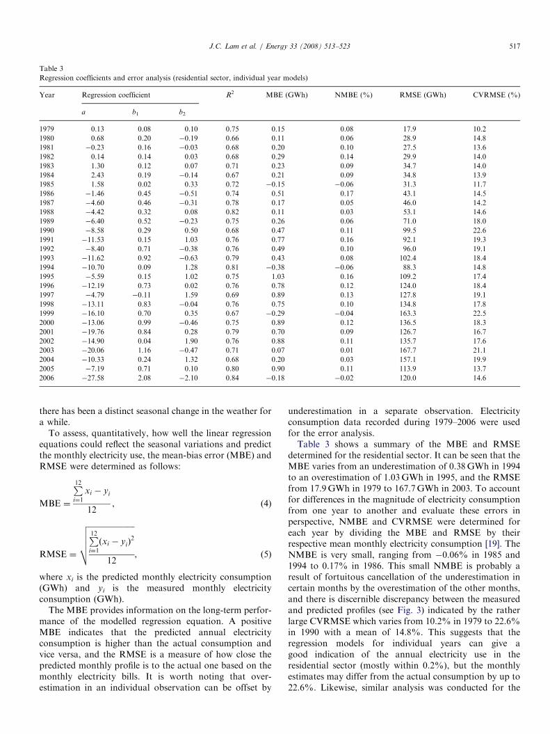
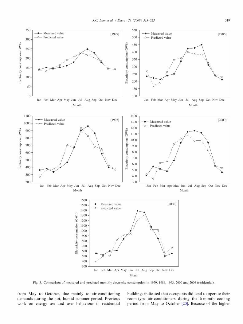
To account for the difference in the number of days in acalendar month, the monthly electricity use in the entiresector was divided by the number of days in that month.Tables 3 and 4 show a summary of the regressioncoefficients (a, b1 and b2) and the coefficients of determina-tion (R2) for the residential and commercial sectors,respectively. It can be seen from Table 3 that R2 variesfrom 0.66 in 1980 to 0.84 in 2006 with a 28-year mean of0.74, and the correlations are considered reasonably strongfor the residential sector. All but the early years (1979, 1980and 1982–1985) have negative intersections when Z1 andZ2 are zero (i.e. negative coefficient ‘‘a’’). There is nodistinct pattern indicating that yearly models with negativeintersections would have better or worse correlation(in terms of larger/smaller R2, normalised mean-bias error(NMBE) and coefficient of variation of the root-mean-square error (CVRMSE)). There seems to be no particularsignificance, physical and otherwise except that in general,negative intersections tend to have comparatively largercoefficients b1 and b2 so, when multiplied by thecorresponding Z1 and Z2, the resulting monthly electricityuse would be positive. There appears to be significantimprovements in the R2 for the commercial sector positiveintersections in all the 28 years (Table 4). R2 varies from0.78 in 1987 to 0.96 in 2006 with a mean of 0.87. FromEq. (3), predicted monthly electricity consumption wasdetermined and compared with the corresponding mea-sured data. Figs. 3 and 4 show the measured and predictedmonthly electricity use profiles in 1979, 1986, 1993, 2000and 2006 for the residential and commercial sectors,respectively. It can be seen that, in general, the predictedconsumption profiles tend to follow the measured onesquite well in terms of the seasonal trends. Not surprisingly,the commercial sector with its larger R2 appears to havebetter agreement between the measured and predicted data.There seems to be a slight phase shift between the twomonthly profiles and the regression models tend tooverestimate for the first half of the year and underestimatefor the second half. We believe that this time lag could havesomething to do with building thermal mass and userbehaviour, in that occupants (especially in the residentialsector) tend to operate their air-conditioning systems after

ARTICLE IN PRESS

Table 3

Regression coefficients and error analysis (residential sector, individual year models)

Year Regression coefficient R2 MBE (GWh) NMBE (%) RMSE (GWh) CVRMSE (%)

a b1 b2

1979 0.13 0.08 0.10 0.75 0.15 0.08 17.9 10.2

1980 0.68 0.20 �0.19 0.66 0.11 0.06 28.9 14.8

1981 �0.23 0.16 �0.03 0.68 0.20 0.10 27.5 13.6

1982 0.14 0.14 0.03 0.68 0.29 0.14 29.9 14.0

1983 1.30 0.12 0.07 0.71 0.23 0.09 34.7 14.0

1984 2.43 0.19 �0.14 0.67 0.21 0.09 34.8 13.9

1985 1.58 0.02 0.33 0.72 �0.15 �0.06 31.3 11.7

1986 �1.46 0.45 �0.51 0.74 0.51 0.17 43.1 14.5

1987 �4.60 0.46 �0.31 0.78 0.17 0.05 46.0 14.2

1988 �4.42 0.32 0.08 0.82 0.11 0.03 53.1 14.6

1989 �6.40 0.52 �0.23 0.75 0.26 0.06 71.0 18.0

1990 �8.58 0.29 0.50 0.68 0.47 0.11 99.5 22.6

1991 �11.53 0.15 1.03 0.76 0.77 0.16 92.1 19.3

1992 �8.40 0.71 �0.38 0.76 0.49 0.10 96.0 19.1

1993 �11.62 0.92 �0.63 0.79 0.43 0.08 102.4 18.4

1994 �10.70 0.09 1.28 0.81 �0.38 �0.06 88.3 14.8

1995 �5.59 0.15 1.02 0.75 1.03 0.16 109.2 17.4

1996 �12.19 0.73 0.02 0.76 0.78 0.12 124.0 18.4

1997 �4.79 �0.11 1.59 0.69 0.89 0.13 127.8 19.1

1998 �13.11 0.83 �0.04 0.76 0.75 0.10 134.8 17.8

1999 �16.10 0.70 0.35 0.67 �0.29 �0.04 163.3 22.5

2000 �13.06 0.99 �0.46 0.75 0.89 0.12 136.5 18.3

2001 �19.76 0.84 0.28 0.79 0.70 0.09 126.7 16.7

2002 �14.90 0.04 1.90 0.76 0.88 0.11 135.7 17.6

2003 �20.06 1.16 �0.47 0.71 0.07 0.01 167.7 21.1

2004 �10.33 0.24 1.32 0.68 0.20 0.03 157.1 19.9

2005 �7.19 0.71 0.10 0.80 0.90 0.11 113.9 13.7

2006 �27.58 2.08 �2.10 0.84 �0.18 �0.02 120.0 14.6

J.C. Lam et al. / Energy 33 (2008) 513–523 517

there has been a distinct seasonal change in the weather fora while.

To assess, quantitatively, how well the linear regressionequations could reflect the seasonal variations and predictthe monthly electricity use, the mean-bias error (MBE) andRMSE were determined as follows:

MBE ¼

P12i¼1

xi � yi

12, (4)

RMSE ¼

ffiffiffiffiffiffiffiffiffiffiffiffiffiffiffiffiffiffiffiffiffiffiffiffiP12i¼1

ðxi � yiÞ2

12

vuuut, (5)

where xi is the predicted monthly electricity consumption(GWh) and yi is the measured monthly electricityconsumption (GWh).

The MBE provides information on the long-term perfor-mance of the modelled regression equation. A positiveMBE indicates that the predicted annual electricityconsumption is higher than the actual consumption andvice versa, and the RMSE is a measure of how close thepredicted monthly profile is to the actual one based on themonthly electricity bills. It is worth noting that over-estimation in an individual observation can be offset by

underestimation in a separate observation. Electricityconsumption data recorded during 1979–2006 were usedfor the error analysis.Table 3 shows a summary of the MBE and RMSE

determined for the residential sector. It can be seen that theMBE varies from an underestimation of 0.38GWh in 1994to an overestimation of 1.03GWh in 1995, and the RMSEfrom 17.9GWh in 1979 to 167.7GWh in 2003. To accountfor differences in the magnitude of electricity consumptionfrom one year to another and evaluate these errors inperspective, NMBE and CVRMSE were determined foreach year by dividing the MBE and RMSE by theirrespective mean monthly electricity consumption [19]. TheNMBE is very small, ranging from �0.06% in 1985 and1994 to 0.17% in 1986. This small NMBE is probably aresult of fortuitous cancellation of the underestimation incertain months by the overestimation of the other months,and there is discernible discrepancy between the measuredand predicted profiles (see Fig. 3) indicated by the ratherlarge CVRMSE which varies from 10.2% in 1979 to 22.6%in 1990 with a mean of 14.8%. This suggests that theregression models for individual years can give agood indication of the annual electricity use in theresidential sector (mostly within 0.2%), but the monthlyestimates may differ from the actual consumption by up to22.6%. Likewise, similar analysis was conducted for the

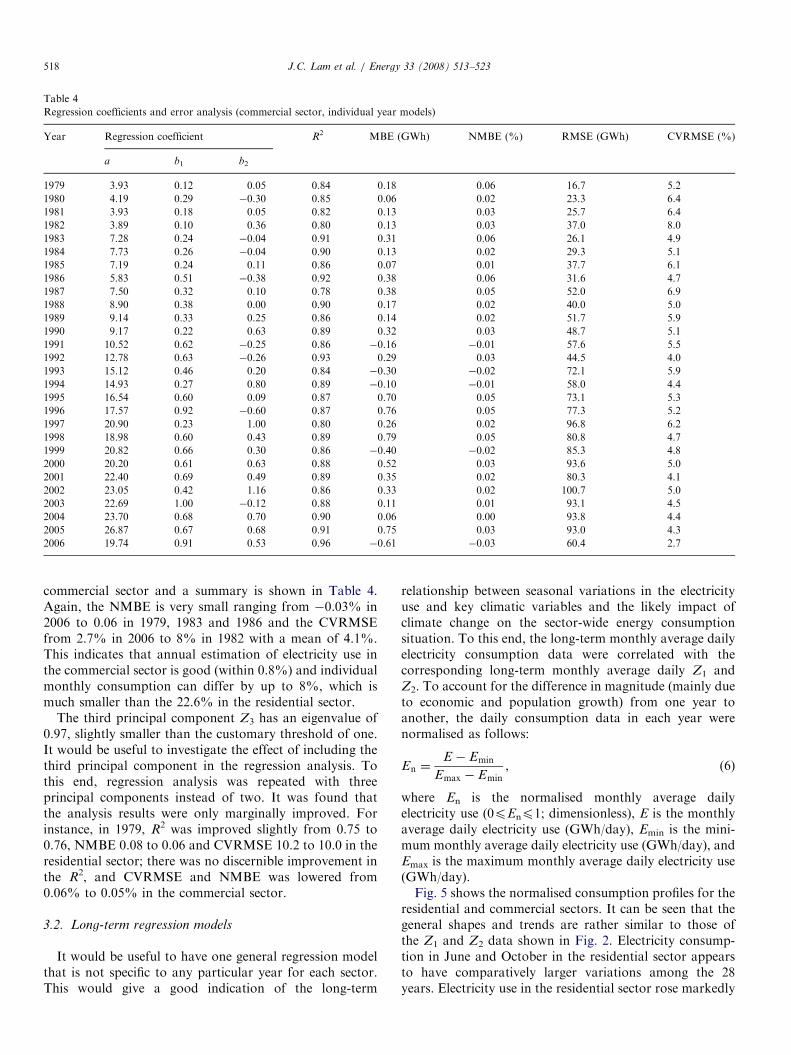
ARTICLE IN PRESS

Table 4

Regression coefficients and error analysis (commercial sector, individual year models)

Year Regression coefficient R2 MBE (GWh) NMBE (%) RMSE (GWh) CVRMSE (%)

a b1 b2

1979 3.93 0.12 0.05 0.84 0.18 0.06 16.7 5.2

1980 4.19 0.29 �0.30 0.85 0.06 0.02 23.3 6.4

1981 3.93 0.18 0.05 0.82 0.13 0.03 25.7 6.4

1982 3.89 0.10 0.36 0.80 0.13 0.03 37.0 8.0

1983 7.28 0.24 �0.04 0.91 0.31 0.06 26.1 4.9

1984 7.73 0.26 �0.04 0.90 0.13 0.02 29.3 5.1

1985 7.19 0.24 0.11 0.86 0.07 0.01 37.7 6.1

1986 5.83 0.51 �0.38 0.92 0.38 0.06 31.6 4.7

1987 7.50 0.32 0.10 0.78 0.38 0.05 52.0 6.9

1988 8.90 0.38 0.00 0.90 0.17 0.02 40.0 5.0

1989 9.14 0.33 0.25 0.86 0.14 0.02 51.7 5.9

1990 9.17 0.22 0.63 0.89 0.32 0.03 48.7 5.1

1991 10.52 0.62 �0.25 0.86 �0.16 �0.01 57.6 5.5

1992 12.78 0.63 �0.26 0.93 0.29 0.03 44.5 4.0

1993 15.12 0.46 0.20 0.84 �0.30 �0.02 72.1 5.9

1994 14.93 0.27 0.80 0.89 �0.10 �0.01 58.0 4.4

1995 16.54 0.60 0.09 0.87 0.70 0.05 73.1 5.3

1996 17.57 0.92 �0.60 0.87 0.76 0.05 77.3 5.2

1997 20.90 0.23 1.00 0.80 0.26 0.02 96.8 6.2

1998 18.98 0.60 0.43 0.89 0.79 0.05 80.8 4.7

1999 20.82 0.66 0.30 0.86 �0.40 �0.02 85.3 4.8

2000 20.20 0.61 0.63 0.88 0.52 0.03 93.6 5.0

2001 22.40 0.69 0.49 0.89 0.35 0.02 80.3 4.1

2002 23.05 0.42 1.16 0.86 0.33 0.02 100.7 5.0

2003 22.69 1.00 �0.12 0.88 0.11 0.01 93.1 4.5

2004 23.70 0.68 0.70 0.90 0.06 0.00 93.8 4.4

2005 26.87 0.67 0.68 0.91 0.75 0.03 93.0 4.3

2006 19.74 0.91 0.53 0.96 �0.61 �0.03 60.4 2.7


commercial sector and a summary is shown in Table 4.Again, the NMBE is very small ranging from �0.03% in2006 to 0.06 in 1979, 1983 and 1986 and the CVRMSEfrom 2.7% in 2006 to 8% in 1982 with a mean of 4.1%.This indicates that annual estimation of electricity use inthe commercial sector is good (within 0.8%) and individualmonthly consumption can differ by up to 8%, which ismuch smaller than the 22.6% in the residential sector.

The third principal component Z3 has an eigenvalue of0.97, slightly smaller than the customary threshold of one.It would be useful to investigate the effect of including thethird principal component in the regression analysis. Tothis end, regression analysis was repeated with threeprincipal components instead of two. It was found thatthe analysis results were only marginally improved. Forinstance, in 1979, R2 was improved slightly from 0.75 to0.76, NMBE 0.08 to 0.06 and CVRMSE 10.2 to 10.0 in theresidential sector; there was no discernible improvement inthe R2, and CVRMSE and NMBE was lowered from0.06% to 0.05% in the commercial sector.

3.2. Long-term regression models

It would be useful to have one general regression modelthat is not specific to any particular year for each sector.This would give a good indication of the long-term

relationship between seasonal variations in the electricityuse and key climatic variables and the likely impact ofclimate change on the sector-wide energy consumptionsituation. To this end, the long-term monthly average dailyelectricity consumption data were correlated with thecorresponding long-term monthly average daily Z1 andZ2. To account for the difference in magnitude (mainly dueto economic and population growth) from one year toanother, the daily consumption data in each year werenormalised as follows:

En ¼E � Emin

Emax � Emin, (6)

where En is the normalised monthly average dailyelectricity use (0pEnp1; dimensionless), E is the monthlyaverage daily electricity use (GWh/day), Emin is the mini-mum monthly average daily electricity use (GWh/day), andEmax is the maximum monthly average daily electricity use(GWh/day).Fig. 5 shows the normalised consumption profiles for the

residential and commercial sectors. It can be seen that thegeneral shapes and trends are rather similar to those ofthe Z1 and Z2 data shown in Fig. 2. Electricity consump-tion in June and October in the residential sector appearsto have comparatively larger variations among the 28years. Electricity use in the residential sector rose markedly

ARTICLE IN PRESS


50

100

150

200

250

300

350[1979] [1986]

[1993]

[2006]

[2000]

Ele

ctri

city

con

sum

ptio

n (G

Wh)

Month

Measured valuePredicted value






150

200

250

300

350

400

450

500

550

Ele

ctri

city

con

sum

ptio

n (G

Wh)

Month


300

400

500

600

700

800

900

1000

1100

Ele

ctri

city

con

sum

ptio

n (G

Wh)

Month


400

500

600

700

800

900

1000

1100

1200

1300

1400

Ele

ctri

city

con

sum

ptio

n (G

Wh)

Month


400

300

500

600

700

800

900

1000

1100

1200

1300

1400

1500

1600

Ele

ctri

city

con

sum

ptio

n (G

Wh)

Month

Fig. 3. Comparison of measured and predicted monthly electricity consumption in 1979, 1986, 1993, 2000 and 2006 (residential).


from May to October, due mainly to air-conditioningdemands during the hot, humid summer period. Previouswork on energy use and user behaviour in residential

buildings indicated that occupants did tend to operate theirroom-type air-conditioners during the 6-month coolingperiod from May to October [20]. Because of the higher

ARTICLE IN PRESS


250

300

350

400

450

500

Ele

ctri

city

con

sum

ptio

n (G

Wh)

Month

Measured valuePredictedvalue






450

500

550

600

650

700

750

800

850

900

Ele

ctri

city

con

sum

ptio

n (G

Wh)

Month


900

800

1000

1100

1200

1300

1400

1500

1600

Ele

ctri

city

con

sum

ptio

n (G

Wh)

Month


1400

1500

1600

1700

1800

1900

2000

2100

2200

2300

2400

Ele

ctri

city

con

sum

ptio

n (G

Wh)

Month


1600

1700

1800

1900

2000

2100

2200

2300

2400

2500

2600

2700

2800

2900

Ele

ctri

city

con

sum

ptio

n (G

Wh)

Month

[1979] [1986]

[1993]

[2006]

[2000]

Fig. 4. Comparison of measured and predicted monthly electricity consumption in 1979, 1986, 1993, 2000 and 2006 (commercial).


internal loads such as people, electric lighting andequipment, the commercial sector tends to have a widermonthly spread indicating a longer cooling season than the

residential sector. Electricity use rose from April toNovember, the 8-month cooling season for commercialbuildings (offices and shopping complexes) in subtropical

ARTICLE IN PRESS


0.0

0.2

0.4

0.6

0.8

1.0[Residential]

[Commercial]

Nor

mal

ised

mon

thly

ave

rage

daily

ele

ctri

city

use

Month


0.0

0.2

0.4

0.6

0.8

1.0

Nor

mal

ised

mon

thly

ave

rage

daily

ele

ctri

city

use

Month

Fig. 5. Normalised monthly average daily electricity use (1979–2006).

Table 5

Summary of error analysis (residential sector, long-term model)

Year MBE (GWh) NMBE (%) RMSE (GWh) CVRMSE (%)

2000 �52.20 �7.00 150.9 20.2

2001 �9.84 �1.30 137.3 18.1

2002 18.81 2.43 153.3 19.8

2003 �30.91 �3.89 177.6 22.3

2004 11.61 1.47 164.1 20.8

2005 �38.56 �4.65 122.3 14.8

2006 33.54 4.09 158.0 19.3

Table 6

Summary of error analysis (commercial sector, long-term model)

Year MBE (GWh) NMBE (%) RMSE (GWh) CVRMSE (%)

2000 6.29 0.34 101.6 5.5

2001 23.01 1.18 105.5 5.4

2002 4.33 0.21 113.5 5.6

2003 22.30 1.08 106.1 5.2

2004 16.53 0.78 101.7 4.8

2005 �16.21 �0.75 96.4 4.5

2006 �5.82 �0.26 74.3 3.4


Hong Kong [21,22]. Multiple regression analysis of thenormalised electricity consumption and the correspondingZ1 and Z2 were conducted for the commercial andresidential sectors. In order to test the predictive capabilityof the long-term models, a limited data set (21-year,1919–1999) was used in the regression, and the remaining7-year data set (2000–2006) for the model evaluation anderror analysis. The resulting regression models are asfollows:

EnðResidentialÞ ¼ �1:0208þ 0:0251� Z1 þ 0:0128� Z2,

(7)

EnðCommercialÞ ¼ �0:9732þ 0:0279� Z1 þ 0:0105� Z2.

(8)

The R2 is 0.69 and 0.84 for the residential andcommercial sectors, respectively, slightly smaller than the0.74 and 0.87 mean R2 for the individual year models.Nevertheless, reasonably strong correlations can still beobserved. Eqs. (7) and (8) were used to predict monthlyelectricity use for the residential and commercial sectorsduring the 7-year period from 2000 to 2006 and an erroranalysis was conducted comparing predictions withthe measured consumption, and a summary is shown in

Tables 5 and 6, respectively. It can be seen that the MBEsare much larger than those of the individual year models(see Tables 3 and 4) indicating less cancellation betweenoverestimation and underestimation. The RMSEs, how-ever, are only slightly larger than those of the individualyear models suggesting that long-term and individual yearmodels show rather similar correlations of the overalltrends of seasonal variation in electricity use. In theresidential sector, NMBE varies from �7% in 2000 to4.09% in 2006 and CVRMSE from 14.8% in 2005 to22.3% in 2003 with a mean CVRMSE of 19.3%. Thissuggests that errors in the estimation of annual andindividual monthly consumption can be up to about 7%and 22%, respectively. Again, the commercial sector showsbetter prediction results with the NMBE ranging from�0.75% in 2005 to 1.18% in 2001 and the CVRMSE from3.4% in 2006 to 5.6% in 2002, indicating, respectively, upto 98% and 94% accuracy in the annual and monthlyconsumption estimation. It should be pointed out thatEqs. (7) and (8) could only estimate the monthly variationswith different climatic indicators not the actual consump-tion forecast for future years.

4. Periods of record and yearly variations in the local

climates

It had been shown that the periods of record could affectthe selection of prevailing weather conditions for air-conditioning requirement analysis and helped detect anyunderlying trend of changing climatic characteristics [23].Earlier work on long-term (1961–2000) ambient tempe-rature in Hong Kong revealed a slight increase in theannual cooling degree-days and suggested that cooling

ARTICLE IN PRESSJ.C. Lam et al. / Energy 33 (2008) 513–523522

requirements, hence energy use for air-conditioning couldbe significantly affected if such trend persisted [24]. In thisstudy, an attempt was made to ascertain any variations inthe climatic indicators (i.e. the principal components Z1

and Z2) during the 1979–2006. Four periods wereconsidered, namely 1979–1985, 1986–1992, 1993–2000and 2000–2006, and a summary of the mean values duringthose periods is shown in Fig. 6. The first principalcomponent Z1 rose slightly from 45.4 during 1979–1985 to46.8 during 2000–2006, and Z2 from 19.1 to 19.6. When theannual mean Z1 and Z2 were considered an increasingtrend (though rather small and gradual) could be detected.Fig. 7 shows the yearly variations of Z1 and Z2 during1979–2006. Z1 varied from 44.8 in 1984 to 47.4 in 2002 witha mean of 46.1, and Z2 from 18.5 in 1986 to 20.6 in 1998with mean of 19.4. Variations from one year to anotherwere small. Z1 and Z2 had a standard deviation of 0.74and 0.51 representing, respectively, 2% and 3% of thecorresponding mean values. The slightly increasing trend

1979-1985 1986-1992 1993-1999 2000-20060

10

20

30

40

50

60

Z1,

Z2

Period of record

Z1 Z2

Fig. 6. Mean Z1 and Z2 during four periods of record.

1980 1985 1990 1995 2000 20051617181920212223

4243

4445

4647

4849

Z2

Z1,

Z2

Year

Z1

Fig. 7. Variations of the annual average Z1 and Z2 during 1979–2006.

had a slope of 0.053 and 0.031 for Z1 and Z2, respectively.Although the increase was small, if this trend persists itcould affect future air-conditioning requirements andhence energy use. Given the growing concern about climatechange, this could have serious energy and environmentalimplications.

5. Conclusions

There has been substantial growth in energy use in HongKong, especially electricity consumption for air-condition-ing in the residential and commercial sectors during thehot, humid summer months. PCA of five climaticvariables—DBT, WBT, global solar radiation, clearnessindex and wind speed—was conducted and two principalcomponents (climatic indicators) were identified, whichrepresent the variations in the prevailing weather condi-tions. Measured sector-wide electricity consumption wascorrelated with the corresponding two principal compo-nents determined using multiple regression technique.Seasonal variations in the monthly electricity consumptionin the commercial sector tended to follow those of theprincipal components more closely than the residentialsector. In general, the regression models tend to showreasonably strong correlation with R2 ranging from 0.66 to0.84 for the residential sector and from 0.78 to 0.96 for thecommercial sector. The regression models could give a verygood indication of the annual electricity use (largely withina few percents), but individual monthly estimation coulddiffer by up to 24%. It was also found that the climaticindicators determined appeared to show a slight increasingtrend during the 28-year period indicating a subtle,but gradual change of climatic conditions that mightaffect future air-conditioning requirements. If this trendpersists, it could have serious energy and environmentalimplications.

Acknowledgements

The work described in this paper was fully supported bya grant from City University of Hong Kong (Project no.7002024). H.L. Tang was supported by a City University ofHong Kong Studentship. Weather data was obtained fromthe Hong Kong Observatory of the Hong Kong SAR.

References

[1] Hong Kong energy statistics annual report. Hong Kong SAR, China:

Census and Statistics Department, 1979–2006. See also: /http://

www.censtatd.gov.hkS.

[2] Hong Kong monthly digest of statistics. Hong Kong SAR, China:

Census and Statistics Department, 1979–2006. See also: /http://

www.censtatd.gov.hkS.

[3] Intergovernmental Panel on Climate Change (IPCC) Working Group

I: The physical basis of climate change, /http://ipcc-wg1.ucar.edu/

wg1/wg1-report.html/S; 2007.

[4] Mayer LS, Benjamini Y. Modeling residential demand for natural gas

as a function of the coldness of the month. Energy Build 1977/

78;1(3):301–12.

http://www.censtatd.gov.hk




http://ipcc-wg1.ucar.edu/wg1/wg1-report.html/

http://ipcc-wg1.ucar.edu/wg1/wg1-report.html/

ARTICLE IN PRESSJ.C. Lam et al. / Energy 33 (2008) 513–523 523

[5] Le Comte DM, Warren HE. Modeling the impact of summer

temperatures on national electricity consumption. J Appl Meteorol

1981;20(12):1415–9.

[6] Sailor DJ, Munoz JR. Sensitivity of electricity and natural gas

consumption to climate in the USA—methodology and results for

eight states. Energy 1997;22(10):987–98.

[7] Sailor DJ, Rosen JN, Munoz JR. Natural gas consumption and

climate: a comprehensive set of predictive state-level models for the

United States. Energy 1998;23(2):91–103.

[8] Mirasgedis S, Sarafidis Y, Georgopoulou E, Lalas DP, Moschovits

M, Karagiannis F, et al. Models for mid-term electricity demand

forecasting incorporating weather influences. Energy 2006;31(3):

208–27.

[9] Lam JC. Climatic and economic influences on residential electricity

consumption. Energy Convers Manage 1998;39(7):623–9.

[10] Yan YY. Climate and residential electricity consumption in Hong

Kong. Energy 1998;23(1):17–20.

[11] Hadley DL. Daily variations in HVAC system electrical energy

consumption in response to different weather conditions. Energy

Build 1993;19(3):235–47.

[12] Lam JC, Wan KKW, Cheung KL, Yang L. Principal component

analysis of electricity use in office buildings. Energy Build, 2007, in

press, doi:10.1016/j.enbuild.2007.06.001.

[13] Wilks DS. Statistical method in the atmospheric sciences: an

introduction. San Diego: Academic Press; 1995.

[14] Storch HV, Zwiers FW. Statistical analysis in climate research.

Cambridge: Cambridge University Press; 1999.

[15] Lam JC. Energy analysis of commercial buildings in subtropical

climates. Build Environ 2000;35(1):19–26.

[16] Lam JC, Lun IYF, Li DHW. Long-term wind speed statistics and

implications for outside surface thermal resistance. Archit Sci Rev

2000;43(2):95–100.

[17] Kalkstein LS, Tan G, Skindlov JA. An evaluation of three clustering

procedures for use in synoptic climatological classification. J Climate

Appl Meteorol 1987;26(6):717–30.

[18] Ladd JW, Driscoll DM. A comparison of objective and subjective

means of weather typing: an example from West Texas. J Appl

Meteorol 1980;19(6):691–704.

[19] M&V guidelines: measurement and verification for federal projects.

Version 2.2. Calibrated computer simulation analysis. Washington,

DC: Department of Energy, 2000 [Chapter 25].

[20] Lam JC. A survey of electricity consumption and user behaviour in

some government staff quarters. Build Res Inf 1993;21(2):109–16.

[21] Lam JC, Li DHW. Electricity consumption characteristics in shopping

malls in subtropical climates. Energy Convers Manage 2003;44(9):1391–8.

[22] Lam JC, Chan RYC, Tsang CL, Li DHW. Electricity use

characteristics of purpose-built office buildings in subtropical

climates. Energy Convers Manage 2004;45(6):829–44.

[23] Colliver DG, Gates RS. Effect of data period-of-record on estimation

of HVAC&R design temperatures. ASHRAE Trans 2000;106(2):

466–74.

[24] Lam JC, Tsang CL, Li DHW. Long-term ambient temperature

analysis and energy use implications in Hong Kong. Energy Convers

Manage 2004;45(3):315–27.

dx.doi.org/10.1016/j.enbuild.2007.06.001

seasonal variations in residential and commercial sector electricity consumption in hong kong

Documents