Submitted 21 March 2017Accepted 16 January 2018Published 27 February 2018

Corresponding authorJacqueline S. Silva-Cavalcanti,jacque_ss@hotmail.com

Academic editorRudiger Bieler

Additional Information andDeclarations can be found onpage 19

DOI 10.7717/peerj.4332

Copyright2018 Silva-Cavalcanti et al.

Distributed underCreative Commons CC-BY 4.0

OPEN ACCESS

Seasonal variation in the abundance anddistribution of Anomalocardia flexuosa(Mollusca, Bivalvia, Veneridae) in anestuarine intertidal plainJacqueline S. Silva-Cavalcanti1,2, Monica F. Costa2 and Luis H.B. Alves2

1Unidade Academica do Cabo de Santo Agostinho (UACSA), Universidade Federal Rural de Pernambuco,Cabo de Santo Agostinho, Pernambuco, Brazil, Pernambuco, Brazil

2Departamento de Oceanografia, Universidade Federal de Pernambuco, Recife, Pernambuco, Brasil,Pernambuco, Brazil

ABSTRACTSpatial and temporal density and biomass of the infaunal mollusk Anomalocardiaflexuosa (Linnaeus, 1767) evaluated a tidal plain at Goiana estuary (Northeast Brazil).Three hundred and sixty core samples were taken during an annual cycle from threeintertidal habitats (A, B andC). Shell ranged from 2.20 to 28.48mm (15.08± 4.08mm).Recruitment occurred more intensely from January to March. Total (0–1,129 g m−2)differed seasons (rainy and dry), with highest values in the early rainy season(221.0 ± 231.44 g m−2); and lowest values in the late dry season (57.34 ± 97 g m−2).The lowest occurred during the late rainy (319± 259 indm−2) and early dry (496± 607indm−2) seasons. Extreme environmental situations (e.g., river flow, salinity and watertemperature) at the end of each season also affected density ranges (late dry: 0–5,798ind m−2; late rainy: 0–1,170 ind m−2). A. flexuosa in the Goiana estuary presented adominance of juvenile individuals (shell length < 20 mm), with high biomass main therecruitment period. Average shell length, density and biomass values suggest overfishingof the stock unit. A. flexuosa is an important food and income resource along its wholedistribution range. The species was previously also known as Anomalocardia brasiliana(Gmelin, 1791).

Subjects Ecology, Environmental Sciences, Marine Biology, Biological OceanographyKeywords Traditional fisheries, Population dynamics, Size classes, Anomalocardia brasiliana,Estuarine ecology

INTRODUCTIONEstuarine intertidal areas support a large number of clam species of varying ecologicguilds, and therefore have been used by humans as important fishing grounds for millenia.Edible bivalves are widely collected around the World and became the basis of manycoastal communities’ livelihoods (Silva-Cavalcanti & Costa, 2011). On the tropical andsub-tropical littoral of the Eastern South America and Caribbean, Anomalocardia flexuosa(Linnaeus, 1767), an infaunal clam distributed from the Western Indies to Uruguay (Rios,1985), is one of the main shellfish fisheries product, especially from the 19th century.A. flexuosa is an important food and income resource along its whole distribution range.

How to cite this article Silva-Cavalcanti et al. (2018), Seasonal variation in the abundance and distribution of Anomalocardia flexuosa(Mollusca, Bivalvia, Veneridae) in an estuarine intertidal plain. PeerJ 6:e4332; DOI 10.7717/peerj.4332

The species was previously also known as Anomalocardia brasiliana (Gmelin, 1791), ajunior synonym. Anomalocardia brasiliana was recognized as a synonym of a A. flexuosaby Fischer-Piette & Vukadinovic (1977: 45ff). The synonymy was followed by subsequentauthors such as Huber (2010: 719).

Biology, ecology and ethnobiology studies aboutAnomalocardia flexuosa started in 1970s.Important ecological studies were published for São Paulo (Narchi, 1976; Schaeffer-Novelli,1976; Arruda-Soares, Schaeffer-Novelli & Mandelli, 1982; Leonel, Magalhães & Lunneta,1983; Corte et al., 2015), Santa Catarina (Pezzuto & Echternacht, 1999; Boehs & Magalhães,2004; Boehs, Absher & Cruz-Kaled, 2008), Paraíba (Grotta & Lunetta, 1980), Ceará (Araújo& Rocha-Barreira, 2004; Barreira & Araújo, 2005), Pernambuco (Oliveira et al., 2013) andRioGrande doNorte (Rodrigues et al., 2008), covering a climate regimes. Living populationsofA. flexuosa from the Caribbean were also (Monti, Frenkiel & Möueza, 1991;Mouëza, Gros& Frenkiel, 1999). All these studies described the reproductive biology of A. flexuosa, andexplored the biotic and abiotic variables that control the spatio-temporal of size, densityand biomass.

Species living in intertidal habitats present spatio-temporal resulting from interactionsbetween physical (tidal amplitude, sub-aereal exposure, water salinity and substratum)and biological (predation, competition, fisheries and other) factors (Rodil et al., 2008;Magalhães, Freitas & Montaudouin, 2016; Gerwing et al., 2016). Moreover, other variablescan influence the distribution of these organisms, as reproductive behaviour, foodavailability, hydrodynamics, organicmatter in the sediments and a number of combinationsamong them (Araújo & Rocha-Barreira, 2004; Gerwing et al., 2016). In addition, humaninterventions (fisheries) are also a factor that deeply influences the population dynamicsof edible benthic bivalves. In some cases, a population might be exploited for long periods(centuries) and, occasionally, become over-exploited, which will compromise its resilience.This is probably the case of A. flexuosa at many sites (Rodrigues et al., 2008).

Knowledge of spatio-temporal distribution and ecology of these bivalves are basis for theestablishment ofmanaged fisheries (including traditional) and environmentalmanagementactions; therefore, can favour the maintenance of natural stocks and contribute for thesustainable exploitation of this resource (Araújo, 2001). Often, studies are published basedon the dynamics of higly-disturbed population, without comparisons with control-sites.This might make the interpretation and of ecological data more difficult for use inmanagement decisions.

The present study aimed to evaluating the spatio-temporal distribution ofAnomalocardiaflexuosa at Goiana estuary (Northeast Brazil) during an annual cycle. We considering shelllength, density and total biomass in this evaluation. Our hypothesis is that fluctuation ofenvironmental parameters (e.g., salinity, grain size) affects a heavily exploited populationof Anomalocardia flexuosa distribution and other biological variables at different spatialand time (seasons).

Silva-Cavalcanti et al. (2018), PeerJ, DOI 10.7717/peerj.4332 2/23

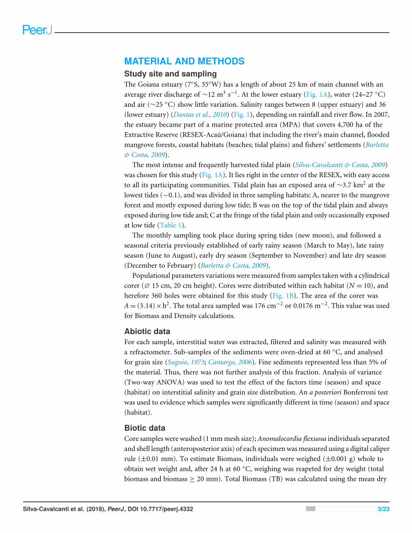
MATERIAL AND METHODSStudy site and samplingThe Goiana estuary (7◦S, 35◦W) has a length of about 25 km of main channel with anaverage river discharge of ∼12 m3 s−1. At the lower estuary (Fig. 1A), water (24–27 ◦C)and air (∼25 ◦C) show little variation. Salinity ranges between 8 (upper estuary) and 36(lower estuary) (Dantas et al., 2010) (Fig. 1), depending on rainfall and river flow. In 2007,the estuary became part of a marine protected area (MPA) that covers 4,700 ha of theExtractive Reserve (RESEX-Acaú/Goiana) that including the river’s main channel, floodedmangrove forests, coastal habitats (beaches; tidal plains) and fishers’ settlements (Barletta& Costa, 2009).

The most intense and frequently harvested tidal plain (Silva-Cavalcanti & Costa, 2009)was chosen for this study (Fig. 1A). It lies right in the center of the RESEX, with easy accessto all its participating communities. Tidal plain has an exposed area of ∼3.7 km2 at thelowest tides (−0.1), and was divided in three sampling habitats: A, nearer to the mangroveforest and mostly exposed during low tide; B was on the top of the tidal plain and alwaysexposed during low tide and; C at the fringe of the tidal plain and only occasionally exposedat low tide (Table 1).

The monthly sampling took place during spring tides (new moon), and followed aseasonal criteria previously established of early rainy season (March to May), late rainyseason (June to August), early dry season (September to November) and late dry season(December to February) (Barletta & Costa, 2009).

Populational parameters variations weremeasured from samples taken with a cylindricalcorer (∅ 15 cm, 20 cm height). Cores were distributed within each habitat (N = 10), andherefore 360 holes were obtained for this study (Fig. 1B). The area of the corer wasA= (3.14)×h2. The total area sampled was 176 cm−2 or 0.0176 m−2. This value was usedfor Biomass and Density calculations.

Abiotic dataFor each sample, interstitial water was extracted, filtered and salinity was measured witha refractometer. Sub-samples of the sediments were oven-dried at 60 ◦C, and analysedfor grain size (Suguio, 1973; Camargo, 2006). Fine sediments represented less than 5% ofthe material. Thus, there was not further analysis of this fraction. Analysis of variance(Two-way ANOVA) was used to test the effect of the factors time (season) and space(habitat) on interstitial salinity and grain size distribution. An a posteriori Bonferroni testwas used to evidence which samples were significantly different in time (season) and space(habitat).

Biotic dataCore samples were washed (1mmmesh size);Anomalocardia flexuosa individuals separatedand shell length (anteroposterior axis) of each specimenwasmeasured using a digital caliperrule (±0.01 mm). To estimate Biomass, individuals were weighed (±0.001 g) whole toobtain wet weight and, after 24 h at 60 ◦C, weighing was reapeted for dry weight (totalbiomass and biomass ≥ 20 mm). Total Biomass (TB) was calculated using the mean dry

Silva-Cavalcanti et al. (2018), PeerJ, DOI 10.7717/peerj.4332 3/23

Figure 1 Study area. (A) Location of the Goiana estuary and position of the tidal plain within the estu-ary. (B–E) Distribution of cores (N = 360) according to season ((B) Late Rainy; (C) Early Dry; (D) LateDry and (E) Early Rainy) and habitats (habitats A, B and C).

Full-size DOI: 10.7717/peerj.4332/fig-1

Silva-Cavalcanti et al. (2018), PeerJ, DOI 10.7717/peerj.4332 4/23

Table 1 Characteristics of each habitat sampled on the tidal plain of the Goiana estuary most used bymussel fishers.

Habitat Main characteristics

A Nearer to the mangrove forest and mostly exposed atlow tide; average altitude 12 m (7 to 16 m) and 750 mwide; Crassostrea rhizhopharae shells buried in sand; LittleAnomaocardia flexuosa fisheries.

B Intermediate area and always exposed during low tide;Average 13 m (10 to 16 m) and 900 m wide; Presence ofHalodule wrightii (seagrass); Intense Anomalocardia flexuosafisheries.

C Fringe of the tidal plain and only occasionally exposedduring low tide; average altitude 11 m (3 to 16 m) and600 m wide; Crassostrea rhizhopharae shells buried in sand;Some Anomalocardia flexuosa fisheries;

weight of the total sampled population. For the purposes of this study, adult individualswere considered those with shell length ≥20 mm (Barreira & Araújo, 2005). Meat dryweight for individuals with shell length > 10 mm was used to calculate the condition Index(CI) and Meat Yield (MY) (Boehs, Absher & Cruz-Kaled, 2008). Field experiments wereapproved by the Federal University of Pernambuco and Enviroment Ministry of Brazil(MMA-IBAMA), IBAMA/Licenca no 21096-1 (2008–2011).

The ANOVA tested for significant differences of shell length and biomass along space(habits A, B and C) and time (seasons). Where ANOVA showed a significant difference,an a posteriori Tukey’s HDS test was used to determine which means were significantlydifferent at the 0.05 level of probability. The Kruskal-Wallis non-parametric analysis ofvariance was used for density analysis. All analyses used STATISTICA (version 8, 2008;StatSoft, Tulsa, OK, USA).

RESULTSAbiotic dataInterstitial salinity was lower during the late rainy season (24.9 ± 0.71), when there isintense rainfall and greater volumes of riverwater reach the low estuary (Table 2). The laterainy season (June –August) presented significant differences (p< 0.05) (Fig. 2). Averagewater salinity was 32.5, 33.2 and 32.7 for the early dry, late dry and early rainy seasons,respectively. Interstitial water salinity did not present significant differences (p≥ 0.05)when the three different are considered.

Significant differences in relation to spatial grain size distribution were not observed.However, there were significant spatial differences among seasons. The late rainy seasonwasdifferent (p< 0.05) from the others. The interaction habitat vs. season was not significant(p≥ 0.05). All habitats (A, B and C) presented dominance of sand, except int the earlyrainy season (Table 3).

Silva-Cavalcanti et al. (2018), PeerJ, DOI 10.7717/peerj.4332 5/23

Figure 2 Salinity of sediments interstitial water. Average and standard deviations salinity of sedimentsinterstitial water on the tidal plain of the Goiana estuary during different seasons (LR, Late Rainy; ED,Early Dry; LD, Late Dry, ER, Early Rainy) and habitats (+= A; • = B; ♦=C). Interaction between seasonvs. habitat: F(6,96)= 0.47035, p= 0.82878.

Full-size DOI: 10.7717/peerj.4332/fig-2

Table 2 Salinity of interstitial water of tidal plain sediments at Goiana estuary at the different habitats(A, B and C) and seasons (n= 9).

Season Average± stdev.

A B C

Late rainy 24.5± 3.13 (n= 9) 25.0± 3.39 (n= 9) 25.3± 2.12 (n= 9)Early dry 31.2± 2.68 (n= 9) 33.7± 1.99 (n= 9) 32.6± 2.00 (n= 9)Late dry 32.1± 1.45 (n= 9) 33.7± 1.48 (n= 9) 33.6± 2.06 (n= 9)Early rainy 31.3± 2.30 (n= 9) 32.8± 2.37 (n= 9) 33.5± 1.58 (n= 9)

Biotic DataA total of 6,770 specimens of A. flexuosa were analysed and had shell between 2.20 and28.48 mm (15.08 ± 4.08 mm). Recruitment was probably continuous, however highernumbers of recruits were registered in the late dry season (January –March) and in earlyrainy season as pointed below (Fig. 3). In respect to size, 1,303 organisms were collectedfrom A, 1,163 were <20 mm of shell length. Adults (shell length > 20 mm) represented9% (2,518) of the individuals in B; and 11.5% in C. Large number of recruits (shelllength < 20 mm) were present in the late dry and early rainy seasons. Two-way ANOVAfound significant differences (p< 0.05) were observed in the interaction between habitatand season vs. size.

Silva-Cavalcanti et al. (2018), PeerJ, DOI 10.7717/peerj.4332 6/23

Table 3 Tidal plain Goiana estuary average sediment characteristics during the different seasons.

Season Area Grain size (%) Sorting Size scale 8

Gravel Sand Silt / clay

1.57 93.68 4.74 Poorly sorted Fine sand 2.350.31 95.4 4.29 Moderately sorted Fine sand 2.900.67 92.95 6.38 Moderately sorted Fine sand 3.022.26 96.73 1.00 Moderately sorted Medium sand 1.706.00 90.12 3.87 Poorly sorted Medium sand 1.752.06 96.18 1.76 Moderately sorted Medium sand 1.911.42 92.56 6.02 Moderately sorted Fine sand 2.743.09 95.68 1.23 Poorly sorted Medium sand 1.23

A

1.60 95.97 2.43 Moderately sorted Medium sand 1.892.69 92.98 4.32 Poorly sorted Medium sand 1.951.49 94.84 3.66 Poorly sorted Fine sand 2.281.87 95.99 2.13 Poorly sorted Fine sand 2.033.60 94.25 2.14 Poorly sorted Medium sand 1.941.89 93.09 5.01 Poorly sorted Fine sand 2.273.09 93.55 3.36 Poorly sorted Fine sand 2.242.34 92.65 4.99 Poorly sorted Fine sand 2.312.35 97.35 0.295 Moderately sorted Medium sand 1.66

B

1.34 94.87 3.788 Poorly sorted Fine sand 2.102.34 95.66 2.00 Poorly sorted Fine sand 2.021.34 93.70 4.95 Poorly sorted Fine sand 2.652.12 93.85 4.02 Poorly sorted Fine sand 2.332.50 91.70 5.84 Poorly sorted Fine sand 2.490.48 95.50 4.03 Poorly sorted Fine sand 1.501.93 90.73 7.34 Poorly sorted Fine sand 2.850.80 96.32 2.87 Moderately sorted Fine sand 2.310.20 95.23 4.57 Moderately sorted Fine sand 2.88

LateRainy

C

2.56 96.51 0.92 Moderately sorted Medium sand 1.873.10 95.11 1.79 Poorly sorted Fine sand 2.166.42 88.02 5.56 Poorly sorted Fine sand 2.195.84 92.26 1.89 Poorly sorted Medium sand 1.481.56 95.5 2.94 Poorly sorted Medium sand 1.771.36 94.3 4.38 Poorly sorted Fine sand 2.275.95 92.6 1.43 Poorly sorted Medium sand 1.081.88 97.83 0.28 Moderately sorted Medium sand 1.691.46 94.84 3.69 Poorly sorted Fine sand 2.22

A

3.68 92.50 3.82 Poorly sorted Medium sand 1.881.84 94.43 3.72 Poorly sorted Fine sand 2.093.41 93.71 2.86 Poorly sorted Medium sand 1.882.33 96.28 1.39 Poorly sorted Medium sand 1.704.71 93.24 2.04 Poorly sorted Medium sand 1.65

(continued on next page)

Silva-Cavalcanti et al. (2018), PeerJ, DOI 10.7717/peerj.4332 7/23

Table 3 (continued)

Season Area Grain size (%) Sorting Size scale 8

Gravel Sand Silt / clay

0.84 94.20 4.96 Poorly sorted Fine sand 2.210.18 94.35 6.36 Poorly sorted Fine sand 2.470.02 99.90 0.01 Well sorted Coarse sand 0.504.91 94.13 0.96 Poorly sorted Medium sand 1.52

B

3.68 95.09 1.23 Poorly sorted Medium sand 1.675.40 93.14 1.45 Poorly sorted Medium sand 1.271.72 98.13 0.14 Moderately sorted Medium sand 1.611.60 96.09 2.30 Poorly sorted Fine sand 2.081.26 97.72 1.01 Poorly sorted Medium sand 1.641.72 95.26 3.02 Poorly sorted Fine sand 2.082.69 95.74 1.56 Poorly sorted Medium sand 1.886.36 92.14 1.50 Poorly sorted Medium sand 1.561.12 95.1 3.80 Poorly sorted Medium sand 2.47

EarlyDry

C

3.25 95.37 1.38 Poorly sorted Fine sand 2.052.46 93.91 3.62 Poorly sorted Fine sand 2.071.32 96.82 1.85 Poorly sorted Medium sand 1.613.24 93.1 3.66 Poorly sorted Fine sand 2.194.77 92.02 3.20 Poorly sorted Medium sand 1.764.39 94.17 1.43 Poorly sorted Medium sand 1.455.22 94.14 0.63 Poorly sorted Medium sand 1.217.24 91.55 1.20 Poorly sorted Coarse sand 0.982.77 95.24 1.98 Poorly sorted Medium sand 1.28

A

2.04 96.59 1.37 Poorly sorted Medium sand 1.4523.2 75.7 1.09 Poorly sorted Coarse sand 0.738.08 89.14 2.77 Poorly sorted Medium sand 1.563.74 92.37 3.88 Poorly sorted Medium sand 1.9210.71 88.16 1.13 Poorly sorted Medium sand 1.314.46 93.77 1.76 Poorly sorted Medium sand 1.675.13 92.48 2.39 Poorly sorted Medium sand 1.603.70 93.48 2.81 Poorly sorted Medium sand 1.51

B

4.70 93.39 1.90 Poorly sorted Medium sand 1.369.07 89.04 1.88 Poorly sorted Medium sand 1.692.85 93.49 3.65 Poorly sorted Fine sand 2.141.97 95.58 2.44 Poorly sorted Fine sand 2.351.45 95.85 2.70 Poorly sorted Fine sand 2.363.52 94.19 2.29 Poorly sorted Medium sand 1.922.98 95.03 1.98 Poorly sorted Fine sand 2.114.63 94.37 0.99 Poorly sorted Medium sand 1.485.06 93.18 1.75 Poorly sorted Medium sand 1.79

LateDry

C

2.82 95.44 1.73 Poorly sorted Fine sand 2.12

(continued on next page)

Silva-Cavalcanti et al. (2018), PeerJ, DOI 10.7717/peerj.4332 8/23

Table 3 (continued)

Season Area Grain size (%) Sorting Size scale 8

Gravel Sand Silt / clay

0 17 83 Very poorly sorted Fine silt 7.320 15.85 84.15 Very poorly sorted Clay 9.320 10.06 89.94 Very poorly sorted Clay 10.580 13.73 86.27 Moderately sorted Clay 12.010 6.84 93.16 Very poorly sorted Clay 10.070 17.7 82.31 Unsorted Coarse clay 8.450 6.74 93.26 Very poorly sorted Clay 11.270 9.27 90.73 Well sorted Clay 12.48

A

0 7.03 15.76 Very poorly sorted Clay 10.530 13.12 86.88 Very poorly sorted Clay 9.260 7.46 92.54 Unsorted Coarse clay 8.620 6.76 93.24 Very poorly sorted Clay 10.580 8.59 91.41 Very poorly sorted Clay 9.660 10.27 89.73 Very poorly sorted Clay 9.730 2.88 97.11 Very poorly sorted Clay 11.010 7.67 92.63 Poorly sorted Clay 11.73

B

0 11.81 88.19 Moderately sorted Clay 11.760 13.13 86.87 Very poorly sorted Clay 9.830 12.74 87.26 Very poorly sorted Clay 10.250 13.28 86.72 Very poorly sorted Clay 11.210 20.67 92.34 Very poorly sorted Clay 10.960 7.66 88.63 Very poorly sorted Clay 10.810 11.36 84.97 Very poorly sorted Clay 10.280 15.03 93.69 Poorly sorted Clay 11.78

EarlyRainy

C

0 6.30 92.40 Very poorly sorted Clay 12.14

Mean density (ind m−2) was 1,600 ± 1,555 in late dry, 1,525 ± 1,389 in early rainy,319 ± 259 in late rainy, and 496 ± 607 in early dry season. The maximum density valuewas lower in the late rainy season (0–1,170 ind m−2) and higher in late dry season (0–5,798ind m−2) (Fig. 4).

The density habitats was lower in C (284 ± 70 ind m−2), A (305 ± 77 ind m−2) andB (369 ± 104 ind m−2) in the late rainy season (Fig. 5). In the early dry season, higherdensity values were found in habitats B (706 ± 525 ind m−2), C (471 ± 376 ind m−2) andA (314 ± 169 ind m−2). Density increased in the late dry season when there were a highnumber of recruits settling on the tidal plain (Fig. 5). Recruitment increased density inhabitats C (2,170 ± 971 ind m−2) and B (1,777 ± 961 ind m−2) (Fig. 5). In the early rainyseason, C (2,060 ind m−2) remained as the most densely populated habitat followed byhabitats B (1,800 ind m−2) and A (706 ind m−2).

Total biomass was higher in early rainy season (221.0 ± 231.44 g m−2) (Fig. 6) inall habitats of the tidal plain (A, B and C). Seasonal Biomass means were 75.6 ± 90.9;57.34 ± 97; 221 ± 231.4 and 23.46 ± 34.39 g m−2 for late rainy, late dry, early rainy and

Silva-Cavalcanti et al. (2018), PeerJ, DOI 10.7717/peerj.4332 9/23

Figure 3 Shell length. Frequency distribution (number of individuals) of shell length (mm) of Anoma-locardia flexuosa at three different habitats (habitat A (A, D, G and J); habitat B (B, E, H and L); habitat C(C, F, I and M)) on a tidal plain of the Goiana estuary during different seasons ((A–C) Late Rainy; (D–F)Early Dry; (G–I) Late Dry; (J–L) Early Rainy).

Full-size DOI: 10.7717/peerj.4332/fig-3

early dry season. The highest Biomass was observed in habitats B (95.5 g m−2) and C(133.25 g m−2) (Fig. 6).

Seven hundred and ninety individuals of A. flexuosa had shell lenght >20 mm. However,adult biomass was lower (0 to 308.5 g m−2) than total biomass (Fig. 7). Adult Biomass(shell length > 20 mm) did not present significant differences among habitats (p> 0.05).Seasonal adult Biomass (shell length > 20 mm) peaked in the late rainy season (43.4 g m−2)when it was responsible for most of TB (90.8, 29.3 and 75.4%) in A, B and C, respectively

Silva-Cavalcanti et al. (2018), PeerJ, DOI 10.7717/peerj.4332 10/23

Figure 4 Density of A. flexuosa. Average and standard deviations density of Anomalocardia flexuosa (indm−1) at a three different habitats (habitats A, B, C) of the tidal plain of the Goiana estuary along differentseasons. (A) Late Rainy; (B) Early Dry; (C) Late Dry; (D) Early Rainy.

Full-size DOI: 10.7717/peerj.4332/fig-4

(Fig. 7). Early rainy season adult Biomass represented between 56 to 78% for estimated TB.Late dry season was when the lowest mean adult Biomass (shell length > 20 mm) occurred(10.8 g m−2 ± 4.32). The adult biomass (shell length > 20 mm) showed differences inrelation to season (p< 0.01), when early and late dry seasons. The interaction betweenseason and habitat showed significant differences (p< 0.05): habitat B during early drywas different from all other habitats and seasons.

There was found spatio-temporal variation in Condition index (CI) and Meat Yield(MY) of A. flexuosa along the year. CI showed significant differences (p< 0.05) for seasonand (Fig. 8A; Table 4). MY were 16.9 ± 10.5% in habitat A, 15.7 ± 10.8% in habitat Band 16.6 ± 13.6% in C (Fig. 8B). Meat yield was significantly correlated to the habitat vs.season interaction (p< 0.05).

DISCUSSIONRainfall patterns determine the occurrence of well-defined seasons (Barletta & Costa,2009). Salinity decreases in the early rainy at Goiana Estuary, ranging from 8 to 36 (Dantaset al., 2010). Water temperature showed the same seasonal trend, with lower temperaturesoccurring in the late rainy (26 ◦C) (Dantas et al., 2010). Rainfall is also responsible for thevariation of interstitial water salinity along different seasons. An increase in the relativeabundance of A. flexuosa was evidenced in the three habitats during the early rainy season.

Silva-Cavalcanti et al. (2018), PeerJ, DOI 10.7717/peerj.4332 11/23

Figure 5 Map of density.Density (ind m−1) of Anomalocardia flexuosa at a tidal plain of the Goiana estu-ary along different seasons (A) Late Rainy; (B) Early Dry; (C) Late Dry; (D) Early Rainy.

Full-size DOI: 10.7717/peerj.4332/fig-5

Silva-Cavalcanti et al. (2018), PeerJ, DOI 10.7717/peerj.4332 12/23

Figure 6 Map of biomass. Total biomass (g m−2) of Anomalocardia flexuosa at a tidal plain in the Goianaestuary along different seasons. (A) Late Rainy; (B) Early Dry; (C) Late Dry; (D) Early Rainy.

Full-size DOI: 10.7717/peerj.4332/fig-6

The grain size changes (sand to clay/silt) can explain the abundance of Anomalocardiaflexuosa during this period. The fine grain predominance favored the A. flexuosa settlingin the different habitats. These results corroborate Rodrigues et al. (2008) that showed anincrease of abundance in this tidal plain where the fine grain size (clay/silt) was dominant.

Silva-Cavalcanti et al. (2018), PeerJ, DOI 10.7717/peerj.4332 13/23

Figure 7 Average and deviations biomass. Average and deviations biomass (shell length > 20 mm) (gm−2) of Anomalocardia flexuosa at three habitats of a tidal of the Goiana estuary along different seasons.(A) Late Rainy; (B) Early Dry; (C) Late Dry; (D) Early Rainy.

Full-size DOI: 10.7717/peerj.4332/fig-7

In this tidal studied in the Goiana estuary there were two cohorts of 3–16 mm and17–23 mm in shell length. This is probably the shell size fishers select either by hand orwith rudimentary tools. The adult organism’s ocurrence was lower along seasons. Thesize distribution shows the presence of more than one cohort, as demonstrated in studiesof species elsewhere. Anomalocardia flexuosa recruitment was probably a reproductivepeak and recruitment phases during early dry and late dry seasons, respectively. Adultbiomass values (shell length > 20 mm) were lower during late dry season and higher inlate rain season (90% total biomass). Similar results were found for Ceará State (Araújo &Rocha-Barreira, 2004). The occurrence of a young cohort (shell length < 20 mm) indicatescontinuous reproduction and a short life cycle. Population dynamics works showed that A.flexuosa longevity ranges between 1.5 to 4.6 years (Monti, Frenkiel & Möueza, 1991; Souza,2007; Rodrigues et al., 2008). Therefore, five years can be considered as the recovered timefor overfished areas, after pressure by capture of this species is diminished or has ceased.Current economic and ecological models proposed that the reduction of fishing effort(e.g., elimination of overfishing and reduced habitat disturbance) could positively affectthe ecosystem and allow economic and social welfare gains (Wang et al., 2016). This wouldbe the case here, since a collapse of the mollusc population might entail grave social risk ofincome reduction for more than 500 families.

Silva-Cavalcanti et al. (2018), PeerJ, DOI 10.7717/peerj.4332 14/23

Figure 8 Meat Yield and Condition Index.Meat Yield (A) and Condition Index (B) average and stan-dard deviations of Anomalocardia flexuosa > 10 mm at the tidal plain (� = A; • = B;� = C) at Goianaestuary along different seasons (LR: Late Rainy; ED: Early Dry; LD: Late Dry and ER; Early Rainy). N =4736 ind. (A: 883; B: 1880; C: 1733), p ≤ 0.05. Interaction season vs. habitat for MY (F(6,4,724) = 2.7116,p= 0.01248) and CI (F(6,4,724)= 3.9232, p= 0.00065).

Full-size DOI: 10.7717/peerj.4332/fig-8

Silva-Cavalcanti et al. (2018), PeerJ, DOI 10.7717/peerj.4332 15/23

Table 4 Kruskal–Wallis analysis for density (ind m−2), Total Biomass, total and adult Biomass (>20mm) (g m−2). ANOVA multifactorial was used for other variables. Differences between habitats vs. seasonwere determined by a post hoc Bonferroni test. NS, Non significant; LR: Late Rainy; ED: Early Dry; LD:Late Dry and ER; Early Rainy; A; B and C are habitats of a tidal plain at Goiana estuary.

Variation Source

Variable Season (1) Habitat (2) Interations

Shell lenght (mm) ** LR ED LD ER ** A B C 1×2**

Total biomass (g m−2) ** LR ED LD IC ER NS NSAdult biomass (shell length >20 mm) (g m−2) ** LR ED LD ER NS 1×2**

Density (ind m−2) * LR ED LD ER NS 1×2**

Condition index (CI) ** LR ED LD ER * A B C 1×2**

Meat yield (MY) * LR ED LD ER NS 1×2*

Notes.*P < 0.05.**P < 0.01.

The settling phase was concentrated during austral summer (September to January),when fishers exert the greater pressure on A. flexuosa stocks, reducing the mature adultpopulation (Silva-Cavalcanti & Costa, 2009). This could help settling by increasing availablespace for recruits, but also sediments turbation by hands and tools can bury recruits andkill them by suffocation, since they would not gain easy access to sediment surface duringhigh tide to filter and feed. According to Boehs, Absher & Cruz-Kaled (2008), more availablespace for recruits can only favour settlers in the late dry season, when reduction of rainfalland reduced predation allow time and space for them to grow.

Abundance in an exploited bivalve population depends on the balance between inputs(reproduction/recruitment and growth) and outputs (mortality and fishery removals)of adult/mature individuals. Reproduction and subsequent succesful recruitment arecrucial for population sustainability (Magalhães, Freitas & Montaudouin, 2016). However,water temperature is only one of the myriad components determining recruitmentsuccess (Magalhães, Freitas & Montaudouin, 2016). In the case of the Goiana estuary,early maturation due to more constant water temperature, even through the rainy season,can also be playing an important role.

Adults (shell length > 20 mm) are preferred by fishers during summer due to meatyield and processing speed (Silva-Cavalcanti & Costa, 2009). In addition, mussel fishingand consumption increases during austral summer, adding non-traditional workers tothe fishing effort, which results in unsustaintable scenarios (Silva-Cavalcanti & Costa,2009). Population mean size (shell length ∼15 mm) at Goiana estuary and other sitessuggests excessive harvesting and catch of individuals bellow maturation size (Araújo,2001; Arruda-Soares, Schaeffer-Novelli & Mandelli, 1982; Boehs et al., 2003). Long-termassessments (∼10 to 20 years) suggest that unsustainable practices in the fisheries of A.flexuosa affect life quality of traditional coastal populations (Silva-Cavalcanti & Costa,2009). Management polices can help reduce overfishing, detain decreases of the populationaverage shell size and finally help increase the abundance of reproductive individuals andrecruitment.

Silva-Cavalcanti et al. (2018), PeerJ, DOI 10.7717/peerj.4332 16/23

The performance of MPAs aimed at traditional fisheries activities depends on severalbiological and ecological factors related to the target species, such as substrate availability,quantity and quality of food resources (i.e., microalgal films) and the degree of overlapwith other species from the same ecological and trophic guilds (Riera et al., 2016). Afactor of utmost importance is regulations enforcement to prevent unplanned harvesting,too common in intertidal areas because of the readly available target species and thelack of refuge (Riera et al., 2016). Tidal plain living resources may reflect an erroneousimpression of commons, as described in community succession models (Gerwing etal., 2016). Optimum size (shell length) to haverst A. flexuosa is suggested at 20 mm(Arruda-Soares, Schaeffer-Novelli & Mandelli, 1982;Barreira & Araújo, 2005)when gonadaldevelopment is reached. However, there are no A. flexuosa above 20 mm (shell length) inAcupe (Bahia State) (Martins & Souto, 2006), for example. Survival of human populationsovercomes ecological concerns (Martins & Souto, 2006) at Goiana estuary, where mostfamilies are below the poverty line, as reflected in very low Human Development Index(IDH) and Education Development Index (IDE) (CPRH, 2003). Thus, A. flexuosa, finfish,mangrove firewood, mangrove crabs and lobsters are exploited without any short orlong-term concerns (Guebert-Bartholo et al., 2011). Shell size of Anomalocardia flexuosa inthe Goiana estuary (mean 15.08 mm ± 4.08 of shell length) was lower than in other areaswith fishing activity (Monti, Frenkiel & Möueza, 1991;Mouëza, Gros & Frenkiel, 1999; Schio,Souza & Pezzuto, 2007; Figueredo & Lavrado, 2007;Mattos, Cardoso & Caetano, 2008; Lima,Barbosa & Correia, 2007; Rodrigues et al., 2013;Morsan, 2007; Boehs et al., 2003). Thus, it ispossible that the population will soon collapse and no longer be able to sustain its fisheriesproduction chain.

TB at Goiana estuary changed along seasons. However, the population structure canbe relatively coupled from the structuring influences of biotic and abiotic factors inthis system. High concentration of resources sustain high density of infauna, and limitexploitative competition reflecting particulary events as namely a ‘‘first come, first served’’process (Gerwing et al., 2016; Magalhães, Freitas & Montaudouin, 2016). The design of theMPA should consider the connectivity among biomass exchanges sites and surroundingareas (Riera et al., 2016).

Density data was compatible with areas considered in expansion or overfishing phases(Castilla & Defeo, 2001; Souza, 2007; Schio, Souza & Pezzuto, 2007). Pirajubaé MarineProtected Area—MPA density values of A. flexuosa ranged from 97 to 203 ind m−2 for shelllength of 19–27 mm and biomass 795 g m−2 (Schio, Souza & Pezzuto, 2007). In the presentwork, biomass ranged from 19 to 338 g m−2, well bellow Pirajubaé and thus, according tothese authors, problaby in the overfishing phase.

Shell size, total wheight and CI were different along the three sampling habitats. Abioticdata were not spatially different. However, capture was different among sampling habitats,A and B being the most used. It is possible that sexually mature individuals from lessernon-exploited areas (ex. C and sub-tidal reaches), kept stocks throughout the Goianaestuary.

The primary effects of size-selective harvesting are the overall reduction in body sizeand an increased mortality rate of harvested species, but other concomitant factors are

Silva-Cavalcanti et al. (2018), PeerJ, DOI 10.7717/peerj.4332 17/23

associated, such as reproductive investment and changes in growth rate and relativefecundity (Riera et al., 2016). Thus, population changes from human intervation aredifficult to assess because there is no information about any unexploited site or controlsite to use as reference. To prevent these processes, it is necessary to develop effectivemanagement strategies to recover limpet populations, such as regulations and the creationof no-take zones.

Condition Index (CI) and Meat Yield (MY) values indicate conversion of glycogen ingametes, sexual maturation and spawning, as well as reflecting the stress and nutritionalstate of A. flexuosa (Absher & Christo, 1993; Aswani et al., 2004; Christo, 2006). Highertemperature and interstitial water salinity, during early and late dry season, stimulatedspawning (Christo, 2006). In this time, in Goiana estuary, gonadal development was over orpartial, thus magnifying the weight of the individual and these two indexes. However, MYwas higher than CI during late rainy season when lower salinity values stressed animals. MYand CI were lowest during early rainy season probably due to spawning. These values weresignificatly different (p≤ 0.05) and suggest that interstitial water salinity and temperatureinfluencied MY and CI. Fisher perceived MY changes along the year and try to profit fromoccasions when it is favourable due to gonadal maturation, thus upsetting the populationright at its reproductive peak (Silva-Cavalcanti & Costa, 2009).

CONCLUSIONThe Goiana estuary has an Anomalocardia flexuosa stock composed mainly of juveniles(<20 mm shell lenght) that its highest biomass during the main recruitment season.Spawning occurs in the late rainy season and might extend up to the late dry season.Interstitial water sanility, temperature and grain size influenced A. flexuosa abundance,and are thus important variables for determining abundance and distribution of thisspecies in the region. Therefore, regulating fisheries might help this overfished populationin different ways, not only by reducing adult/mature biomass removal, but also leavingsediments undisturbed at no-take zones and for longer periods.

Seasonal differences were observed for biomass and density, with the early rainyseason presenting higher values. Theses values suggest that A. flexuosa is overfished. Thereprodution peak was in the late rainy season (June to August). Reproductive cycle anddensity data are important variables for the evaluation of the fishing stocks as well as forthe design and assessment of resource management plans and instruments. Interannualand interdecadal studies about variations in population parameters at control sites willbe important to create standards to compare with sites under anthropogenic interference.These investigations can better estimate, in a medium term (3–5 years), the potentialrecovered of well-managed stocks. This information can then help in deciding aboutlocation and habilitation of new MPAs.

ACKNOWLEDGEMENTSAuthors thank Mr. Antonio dos Santos Alves for his help during the entire fieldwork,companionship and for sharing his knowledge about estuarine ecology and management.

Silva-Cavalcanti et al. (2018), PeerJ, DOI 10.7717/peerj.4332 18/23

Dr. MCB Araújo, MSc. SCT Barbosa-Cintra and E Cavalcanti are aknowledged for theirhelp during field and lab work.

ADDITIONAL INFORMATION AND DECLARATIONS

FundingJacqueline Santos Silva-Cavalcanti was supported by CAPES-Brasil for a PhD scholarshipfrom 2007–2008 and CNPq for the pos-doctoral grant Proc. No. 157563/2015-4. MonicaFerreira da Costa is a CNPq Fellow. The funders had no role in study design, data collectionand analysis, decision to publish, or preparation of the manuscript.

Grant DisclosuresThe following grant information was disclosed by the authors:CAPES-Brasil.CNPq: 157563/2015-4.

Competing InterestsThe authors declare there are no competing interests.

Author Contributions• Jacqueline S. Silva-Cavalcanti conceived and designed the experiments, performed theexperiments, analyzed the data, contributed reagents/materials/analysis tools, wrote thepaper, prepared figures and/or tables.• Monica F. Costa conceived and designed the experiments, performed the experiments,wrote the paper, reviewed drafts of the paper, english corrections.• Luis H.B. Alves performed the experiments, prepared figures and/or tables.

Field Study PermissionsThe following information was supplied relating to field study approvals (i.e., approvingbody and any reference numbers):

Field experiments were approved by the Federal University of Pernambuco andEnviroment Ministry of Brazil (MMA-IBAMA).

Data AvailabilityThe following information was supplied regarding data availability:

The raw data has been supplied as a Supplementary File.

Supplemental InformationSupplemental information for this article can be found online at http://dx.doi.org/10.7717/peerj.4332#supplemental-information.

REFERENCESAbsher TM, Christo SW. 1993. Índice de Condicão de ostras da região entre-marés da

Baía de Paranaguá, Paraná. Arquivos de Biologia e Tecnologia or Brazilian Archives ofBiology and Technology 36(2):253–261.

Silva-Cavalcanti et al. (2018), PeerJ, DOI 10.7717/peerj.4332 19/23

Araújo CMM. 2001. Biologia reprodutiva do berbigão Anomalocardia brasiliana (Gmelin,1791) (Mollusca, Bivalvia, Veneridae) na Reserva Extrativista Marinha de Pirajubaé.Tese de Doutorado, Universidade de São Paulo - Ciências Biológicas (BiologiaGenética.

AraújoMLR, Rocha-Barreira CA. 2004. Distribuicão espacial de Anomalocardiabrasiliana (Gmelin 1791) (Mollusca, Bivalvia, Veneridae) na praia do Canto daBarra, Fortim, Ceará, Brasil. Boletim Técnico do CEPENE 12(1):11–21.

Arruda-Soares H, Schaeffer-Novelli Y, Mandelli J. 1982. Anomalocardia brasiliana(Gmelin, 1791) bivalve comestível da região do Cardoso, Estado de São Paulo:aspectos biológicos de interesse para a pesca comercial. Boletim do Instituto de Pesca9:21–38.

Aswani K, Volety S, Tolley G, Savarese M,Winstead JT. 2004. Role of anthropogenicand environmental variability on the physiological and ecological responses ofoysters in southwest Florida estuaries. Journal of Shellfish Research 23(1):315–316.

Barletta M, Costa M. 2009. Living and non-living resources exploitation in tropical semi-arid estuaries. Journal of Coastal Research 56:371–375.

Barreira CA, AraújoMLR. 2005. Ciclo reprodutivo de Anomalocardia brasiliana (Gmelin1791) (Mollusca, Bivalvia, Veneridae) na praia do canto da Barra, Fortim, Ceará,Brasil. Boletim do Instituto de Pesca 31(1):9–20.

Boehs G, Absher TM, Cruz-Kaled AC. 2008. Ecologia populacional de Anomalocardiabrasiliana (Gmelin, 1791) (Bivalvia, Veneridae) na baia de Paranaguá, Paraná. BrasilBoletim do Instituto de Pesca, São Paulo 34(2):259–270.

Boehs G, Blankeinsteyn A, Alves R, Sabry RC, Carvalho FG, Omingos JAS, Filho JWC.2003.Macrofauna Bêntica de Uma Planície de Maré da Enseada de Ratones, Ilha deSanta Catarina, SC, Brasil. Biotemas 16(2):45–65.

Boehs G, Magalhães ARM. 2004. Simbiontes associados com Anomalocardia brasil-iana (Gmelin, 1791) (Mollusca, Bivalvia, Veneridae) na ilha de Santa Catarina eregião continental adjacente, Santa Catarina, Brasil. Revista Brasileira de Zoologia21(4):865–869 DOI 10.1590/S0101-81752004000400021.

CamargoM. 2006. SYSGRAN: um sistema de código aberto para análises granulométri-cas de sediemento. Revista Brasileira de Geociências 36(2):371–378.

Castilla JC, Defeo O. 2001. Latin American benthic shellfisheries: emphasis on co-management and experimental practices. Reviews in Fish Biology and Fisheries11(1):1–30.

Christo SW. 2006. Biologia Reprodutiva e Ecologia de Ostras do gênero CrassostreaSacco, 1897, na Baía de Guaratuba (Paraná - Brasil): Um Subsídio ao Cultivo.Theses, Universidade Federal do Paraná, Paraná, 146 p.

Companhia Pernambucana doMeio Ambiente (CPRH). 2003.Diagnóstico sócio-ambiental do litoral Norte de Pernambuco. CPRH Publicacões, Recife, 214 pp.Available at http://www.cprh.pe.gov.br/downloads/Folha_de_Rosto_e_Ficha_Catalografica.pdf .

Corte GN, Yokoyama LQ, Coleman RA, Amaral CZ. 2015. Population dynamics of theharvested clam Anomalocardia brasiliana (Bivalvia: Veneridae) in Cidade Beach,

Silva-Cavalcanti et al. (2018), PeerJ, DOI 10.7717/peerj.4332 20/23

south-east Brazil. Journal of the Marine Biologial Association of the United Kingdom95(6):1183–1191 DOI 10.1017/S0025315415000156.

Dantas DV, Barletta M, Costa MF, Barbosa-Cintra SCT, Possatto FE, Ramos JAA, LimaARA, Saint-Paul U. 2010.Movement patterns of catfishes in a tropical semi-arid es-tuary. Journal of Fish Biology 76:2540–2557 DOI 10.1111/j.1095-8649.2010.02646.x.

FigueredoMIS, Lavrado HP. 2007. Estrutura populacional de Anomalocardia brasiliana(Gmelin, 1791) (Mollusca Bivalvia) em uma lagoa hipersalina (Lagoa de Araruama,RJ). In: XII Congresso Latino-Americano de Ciências do Mar. XII COLACMAR,Florianópolis, 15 a 19 de abril de 2007. CD-ROM.

Fischer-Piette É, Vukadinovic D. 1977. Suite des révisions des Veneridae (Moll. Lamel-libr.) Chioninae, Samaranginae et complément aux Vénus.Mémoires du MuséumNational d’Histoire Naturelle (NS), Série A (Zoologie) 106:1–186.

Gerwing TG, Drolet D, Hamilton DJ, BarbeauMA. 2016. Relative importance of bioticand abiotic forces on the composition and dynamics of a soft-sediment intertidalcommunity. PLOS ONE 11(1):e0147098 DOI 10.1371/journal.pone.0147098.

Grotta M, Lunetta JE. 1980. Ciclo sexual de Anomalocardia brasiliana (Gmelin, 1791) dolitoral de Estado de Paraíba. Revista Nordestina de Biologia 3:5–55.

Guebert-Bartholo FM, Barletta M, Costa MF, Lucena LR, Pereira da Silva C. 2011.Fishery and the use of space in a tropical semi-arid estuarine region of NortheastBrazil: subsistence and overexploitation. Journal of Coastal Research 64:398–402.

HuberM. 2010. Compendium of bivalves. A full-color guide to 3,300 of the world’smarine bivalves. In: A status on Bivalvia after 250 years of research. Hackenheim:ConchBooks, 1 CD-ROM, 901 pp.

Leonel RMV,Magalhães ARM, Lunneta JE. 1983. Sobrevivência de Anomalocardiabrasiliana (Gmelin, 1791) (Mollusca: Bivalvia), em diferentes salinidades. Boletimde Fisiologia da Universidade de São Paulo 7:63–72.

Lima HC, Barbosa JM, Correia DS. 2007. Extracão de marisco por moradores dacomunidade de Baira-Mar 2, Igarassu-PE. In: VII Jornada de Ensino, Pesquisa eExtensão. Recife: JEPEX, SP, Adaltech.

Magalhães L, Freitas R, Montaudouin X. 2016. Cockle population dynamics: re-cruitment predicts adult biomass, not the inverse.Marine Biology 163(16)DOI 10.1007/s00227-015-2809-.

Martins VS, Souto FJB. 2006. Uma análise biométrica de bivalves coletados pormarisqueiras no manguezal de Acupe, Santo Amaro, Bahia: uma abordagemetnoconservacionista. Sitienbus Série Ciência Biológicas 6:98–105.

Mattos G, Cardoso RS, Caetano CHS. 2008. Dinâmica populacional de Anomalocardiabrasiliana (Gmelin, 1791) (Bivalvia: Veneridae) na praia das Fleixeiras, Ilha deItacuruca, Rio de Janeiro—Resultados preliminares. In: III Congresso Brasileiro deOceanografia-CBO, I Congresso Ibéro-Americano de Oceanografia, Fortaleza (CE).

Monti D, Frenkiel L, MöuezaM. 1991. Demography and growth of Anomalocardiabrasiliana (Gmelin) Bivalvia: Veneridae in a mangrove in Guadalupe (French WestIndies). Journal of Molluscan Studies 57:249–257 DOI 10.1093/mollus/57.2.249.

Silva-Cavalcanti et al. (2018), PeerJ, DOI 10.7717/peerj.4332 21/23

Morsan E. 2007. Spatial pattern, harvesting and management of artisanal fishery forpurple clam (Amiantis purpurata) in Patagonia (Argentina). Ocean and CoastalManagement 50:481–497 DOI 10.1016/j.ocecoaman.2006.10.001.

MouëzaM, Gros O, Frenkiel L. 1999. Embryonic, larval and postlarval developmentof the tropical clam, Anomalocardia brasiliana (Bivalvia, Veneridae). Journal ofMolluscan Studies 65:73–88 DOI 10.1093/mollus/65.1.73.

NarchiW. 1976. Ciclo anual da gametogênese de Anomalocardia brasiliana (Gmelin,1791) (Mollusca: Bivalvia). Boletim de Zoologia da Universidade de São Paulo1:331–350.

Oliveira L, Lavander H, Rodrigues S, Brito LO, Gálvez O. 2013. Crescimento doberbigão Anomalocardia brasiliana (BIVALVIA:VENERIDAE) na praia de MangueSeco, Pernambuco, Brasil. Arquivos de Ciências do Mar 46(1):22–28.

Pezzuto PR, Echternacht AM. 1999. Avaliacão de impactos da construcão da via expressaSC-Sul sobre o berbigão Anomalocardia brasiliana (Gmelin, 1791) (Mollusca:Pelecypoda) na Reserva Extrativista Marinha do Pirajubaé (Florianópolis, SantaCatarina, Brasil). Atlântica 21:105–119.

Riera R, Perez O, Alvarez O, Simon D, Díaz D, Monterroso O, Nunez J. 2016. Clear re-gression of harvested intertidal mollusks. A 20-year (1994–2014) comparative study.Marine Environmental Research 113:56–61 DOI 10.1016/j.marenvres.2015.11.003.

Rios EC. 1985. Seashells of Brasil. Rio Grande: Fundacao Cidade do Rio Grande,Fundagao Universidade do Rio Grande, Museu Oceanografico, 329 pp., 102 p.

Rodil IF, Cividanes S, Lastra M, López J. 2008. Seasonal variability in the verti-cal 324 distribution of benthic macrofauna and sedimentary organic mat-ter in an estuarine 325 beach (NW Spain). Estuaries and Coasts 31:382–395DOI 10.1007/s12237-007-9017-4.

Rodrigues AML, Borges-Azevedo CM, Costa RS, Henry-Silva GG. 2013. Populationstructure of the bivalve Anomalocardia brasiliana (Gmelin, 1791) in the semi-aridestuarine region of northeastern Brazil. Brazilian Journal of Biology 73:819–833DOI 10.1590/S1519-69842013000400019.

Rodrigues AM,Marques AO, Fernandes RTV, Henry-Silva GH. 2008. Distribuicãoe abundancia do molusco bivalve Anomalocardia brasiliana (Gmelin, 1791) naspraias da região estuarina do rio Apodi/Mossoró/RN. In: III Congresso Brasileiro deOceanografia-CBO 2008, I Congresso Ibéro-Americano de Oceanografia, Fortaleza.

Schaeffer-Novelli Y. 1976. Alguns aspectos ecológicos e análise da populacão de Anoma-locardia brasiliana (Gmelin, 1791) Molusca-Bivalvia na praia do Saco da Ribeira.Ubatuba, Estado de São Paulo. Tese de Doutorado: Instituto de Biociências,Universidade de São Paulo.

Schio C, Souza DS, Pezzuto PR. 2007. Dinâmica populacional do berbigão Anomalo-cardia brasiliana (Gmelin, 1791) (Mollusca: Pelecypoda) na Reserva ExtrativistaMarinha de Pirajubaé-SC, Brasil. In: XII Congresso Latino Americano de Ciências doMar (COLACMAR), 15 a 19 de abril de 2007 (cd-rom).

Silva-Cavalcanti et al. (2018), PeerJ, DOI 10.7717/peerj.4332 22/23

Silva-Cavalcanti JS, Costa M. 2009. Fisheries in Protected and Non-Protected areas:what is the difference? The case of Anomalocardia brasiliana (Gmelin, 1971) (Mol-lusca: Bivalvia) at tropical estuaries of Northeast Brazil. Jounal of Coastal Research56:1454–1458.

Silva-Cavalcanti JS, Costa M. 2011. Fisheries of Anomalocardia brasiliana in tropicalestuaries. Pan-American Journal of Aquatic Sciences 6(2):86–99.

Souza DS. 2007. Caracterizacão da pescaria do berbigão Anomalocardia brasiliana(Gmelin, 1791) (Mollusca: Bivalvia) na Reserva Extrativista Marinha do Pirajubaé(Florianopólis-SC): Subsídios para o manejo. Master’s dissertation, Universidade doVale do Itajaí.

Suguio K. 1973. Introducão à sedimentologia. São Paulo: Edgard Blucher/EDUSP, 317 p.Wang Y, Hu J, Pan H, Li S, Failler P. 2016. An integrated model for marine fishery

management in the Pearl River Estuary: linking socio-economic systems andecosystems.Marine Policy 64:135–147 DOI 10.1016/j.marpol.2015.11.014.

Silva-Cavalcanti et al. (2018), PeerJ, DOI 10.7717/peerj.4332 23/23