SEASONAL STORAGE OF SOLAR ENERGY IN BOREHOLE HEAT EXCHANGERS

Simon Chapuis and Michel Bernier

Département de génie mécanique École Polytechnique de Montréal

Montréal, Québec, Canada

ABSTRACT Seasonal storage of solar energy in geothermal boreholes has resurfaced as a means of heating housing communities. Typically, these systems operate at relatively high temperatures leading to high heat losses from the ground storage volume and to low solar collector efficiencies. In this paper, a new seasonal storage strategy is proposed. First, the storage temperature is kept relatively low in order to limit heat losses and improve solar collector efficiencies. Secondly, the seasonal borehole storage is designed in such a way as to enable simultaneous charging and discharging of the ground using four pipe boreholes with two independent counter-current circuits. Finally, the temperature level is raised using heat pumps to supply heat at an acceptable temperature for space heating. The proposed configuration is simulated with TRNSYS using a modified version of the DST model. Results from simulations indicate that it is possible to keep the seasonal storage temperature at an annual average slightly above the annual mean ambient temperature using a relatively small solar collector area (about 11 m2 per house) leading to relatively high solar collector efficiencies. Combined with a heat pump, it is shown that this system can reach a solar fraction of 78 %.

INTRODUCTION Seasonal storage of solar energy in the ground using multiple boreholes, often referred to as a BTES (Borehole Thermal Energy Storage), has resurfaced as a mean of heating housing communities. Some examples are included in a literature review presented recently in a related study (Chapuis and Bernier, 2008). Such a system has been implemented in a northern climate to heat 52 homes in the town of Okotoks, Alberta, Canada (Sibbitt et al., 2007). This BTES is designed such that the fluid circulation in the boreholes induces a radial thermal stratification in the ground. With this approach the hottest zone is in the center and it can be used directly for space heating.

The BTES is composed of 24 parallel circuits of 6 boreholes in series for a total of 144 boreholes. In charging mode, the fluid is heated by a 2293 m2 solar collector array (about 44 m2 per house). It enters the BTES near the center and it then progresses towards the periphery. In discharging mode, the same pipes are used but the flow direction is reversed. Thus, the fluid enters at the periphery and exists at the center of the BTES. Above ground fluid tanks are also used to provide short-term thermal storage. Early results indicate that the system at Okotoks will reach close to a 100% solar fraction for space heating after an initial 5 years charging period (McDowell & Thornton, 2008). The predicted end of summer BTES temperature is around 80oC. Such a high storage temperature has two drawbacks. First, the return temperature to the solar collectors is relatively high which leads to relatively low solar collector efficiencies. Second, heat losses from the borehole storage are relatively high as they represent 60% of the injected heat (Sibbitt et al., 2007). In this paper a new seasonal storage strategy is proposed. The basic concept used above is retained, i.e. the energy collected by solar collectors is used to charge a seasonal BTES. However, the strategy is to keep the storage temperature at a lower level in order to reduce heat losses and improve solar collector efficiencies.

Figure 1 Schematic representation of the system proposed in this study

As shown in Figure 1, the proposed seasonal BTES is designed in such a way that it enables simultaneous charging and discharging of the ground using two

Eleventh International IBPSA Conference Glasgow, Scotland

July 27-30, 2009

- 599 -

counter-current pipe networks based on 4 pipes boreholes (2 independent U-tubes per borehole). No short-term thermal storage tanks are required. The solar charging network circulates a fluid from the center to the periphery of the BTES while the house heating discharging network circulates a fluid in the opposite direction. Finally, a boiler or a heat pump is used if the supply temperature level is insufficient for space heating. In this study, a modified version of the DST model is proposed to model the counter-current 4 pipe boreholes. Before presenting these modifications, the DST model is reviewed and documented. In the last part of this paper, two case studies, which use the proposed charging/discharging scheme, are presented.

DST MODEL In the present work, the well-known DST model (Duct Ground Heat Storage Model) (Claesson et al., (1981), Hellström (1989), Mazzarella (1989) and Pahud (1996) is modified (it will be referred to as the “modified DST model” in this paper) to accommodate simultaneous charging and discharging in the same borehole. The basis for the DST model used here is TYPE557a (vertical U-tubes/without known borehole thermal resistance) from the TESS libraries (TESS, 2004) used in TRNSYS (Klein, 2004). The following paragraphs illustrate the computational procedure that takes place in the DST model. The DST model is able to predict the amount of heat transferred from a fluid circulating in a borehole to the ground. In all cases, the boreholes are assumed to be uniformly placed in the BTES volume. The heat transfer problem is solved by splitting the problem into simpler problems. Then, using the linearity of the heat conduction equation, various solutions are superposed to obtain the final solution. Central to the DST model is the superposition of two numerical solutions: the so-called Local and Global solutions, both of which are linked by Subregions. Heat transfer between the circulating fluid and the ground is given by an analytical solution applied over borehole segments which is then used as a boundary condition in the Local problem. Finally, a Steady Flux analytical solution redistributes the energy into the BTES ground volume. Mesh networks As shown in Figure 2, the DST model uses three mesh networks referred to as: Subregion, Local and Global. In this example, 19 boreholes are shown with 15 Subregions (3 radial and 5 axial). The DST model can handle a unique number of boreholes connected in series per parallel loop (i.e. all parallel loops have the same number of boreholes connected in series).

The BTES volume, VBTES , has a cylindrical shape. Its radius, RBTES is obtained using Eq.1:

2BTES BTESV R H (1)

where H is the borehole height. The BTES volume is divided into Subregions, using a 2D (r,z) axisymmetric mesh network with respect to the BTES central axis. The number of Subregions (NLOC) equals the number of radial regions times the number of vertical regions, both specified by the user. The vertical heights of the Subregions are defined by an algorithm imposing shorter height meshes on the top and bottom of the BTES where there are steep gradients. So-called Radial regions include one or more Subregions. For example in Figure 2, the radial region closest to the BTES center includes Subregions #1 to #5. The radial length of a radial region is set such that the related surface area it covers has an area proportional to the total number of boreholes assigned by the code in that radial region. Boreholes connected in series per parallel loop are distributed one after the other to the radial regions starting from the BTES center towards the BTES periphery. If there are less radial regions than boreholes connected in series, the distribution resumes from the BTES center. From there, the total number of boreholes per radial region is proportional to the ratio of boreholes connected in series per radial regions. For example, if the user specified a total of 15 boreholes with 5 boreholes connected in series per parallel loop and 3 radial regions, the code will do the following assignments: 2

5 15 boreholes in radial region no.1;

25 15 boreholes in radial region no.2;

15 15 boreholes in radial region no.3.

Then radial region no.3 will cover half the surface area of the other two radial regions. A borehole length, LSub, is assigned to each Subregion. Its value is equal to the number of boreholes in the radial region from which the Subregion belongs times the height of the Subregion. As shown in Figure 2, the Subregions are numbered successively from 1 to NLOC starting from the Subregion located at the bottom left corner of the Subregions network. The fluid circulates into the BTES from Subregions 1 to NLOC if the user specified that the fluid circulates from the center to the border of the BTES or from Subregion NLOC to 1 if the user specified a fluid circulation from the border to the center of the BTES. The Subregion mesh network is used to build a

- 600 -

refined and extended mesh called the Global mesh network (bottom right in Figure 2). This mesh is used to calculate heat transfer occurring inside the BTES as well as between the BTES and its surroundings. The Global network radial and vertical meshes are generated by an algorithm taking into account the ground thermal properties and the number of simulation years as specified by the user. The positions of the Global meshes inside the BTES are defined in such a way that they correspond to Subregion limits. However, the Global mesh can be finer than the Subregion mesh. For example, in Figure 2, there are 2 Global meshes that belong to Subregion no.8. The Global mesh network also extends beyond the BTES volume as follows: i) the length of the first two meshes outside the BTES volume (both in r and z) are equal to twice the penetration depth (Hellström, 1991) for a time period

t; 2 t , where α is the ground thermal diffusivity and t is fixed to 72 hours; ii) the length of the next meshes increases successively by a factor 2 until they reach a distance

greater then 2 t from the BTES radius or bottom, where, in this case, t is the number of simulated years specified by the user; iii) The very last mesh, in r or z direction, is then positioned 100 meters further (fixed value). To each Subregion is also associated a so-called Local mesh network (middle right in Figure 2) that models the heat transfer effects from the fluid circulating in the borehole to the surrounding ground.

Figure 2 Mesh networks used in the DST model (not to scale)

- 601 -

Each Local problem uses a radial mesh network. All Local mesh networks cover a ground region from the borehole radius, R0 (which is user specified), to the radius R1. The radius R1 is obtained from:

2tot1 NBH BTESR H V (2)

where NBHtot is the total number of boreholes. Local mesh networks have all the same dimensions except for the borehole length over which the fluid circulates. The related volume of any Subregion is exactly the same as the one of its Local problem and is defined as:

2 2 2, , , ,1 Sub Sub ext Sub int Sub ext Sub intR L r r z z (3)

Fluid to ground heat transfer Whatever the number of U-tubes per borehole, DST models the fluid circulation in the borehole pipes as if there was only one pipe located in its center. The total user specified fluid flow rate runs over LSub. The thermal effects related to the presence of multiple pipes in a borehole are taken into account by an equivalent thermal resistance, Rb. The resistance Rb covers the domain which includes the fluid, the pipe material and the gap between the borehole and the ground. It is computed by representing each pipe (1 U-tube = 2 pipes) in the borehole as a line source. The assumptions leading to the calculation of Rb are an equal temperature for all line sources and a uniform temperature at the borehole wall, Tb. Rb is calculated once during the initialization process and it remains constant throughout the simulations. Boundary/initial conditions The Local mesh networks boundary conditions are: known heat transfer rate at R0, qLoc,R0 ; zero heat flux at R1.

The Global mesh networks boundary conditions are: user specified (constant or variable) ground

surface temperature; zero heat flux at the BTES center; zero heat flux for the last radial and vertical

meshes.

The Local meshes initial condition is a temperature equal to 0 °C. The Global meshes initial condition is a temperature equal to the initial surface temperature unless the user specifies a period of preheating and a temperature gradient in the ground (caused by the geothermal heat flux). Time steps definitions The heat transfer processes in the Local mesh

networks are computed at each "short" time step dtr (more precisely it is calculated X times during a TRNSYS time step, where X is the rounded up integer value of the TRNSYS time step divided by dtr). The value of dtr is based on the ground thermal properties, the borehole thermal resistance and the dimensions of the Local mesh networks. The heat transfer calculations in the Global mesh network are initiated after a time corresponding to a Fourier number (where Fo = αt/R12) equal to 0.2 (denoted here by tFo=0.2). Then, the calculations are performed at each "long" time step dt (more precisely, at the first TRNSYS time step after dt). Explanations on the rational for the Fo=0.2 selection can be found in Hellström (1991). In a nutshell, it is based on the one-dimensional ground temperature evolution around a borehole for which the boundary conditions are: a constant heat flux at the borehole radius, R0 and a zero heat flux at a radial distance R1 from the borehole. For times prior to tFo=0.2, the ground temperature profile shape between R0 and R1 is variable but becomes constant for times greater than tFo=0.2. After tFo=0.2, the ground temperature at any point in the domain of interest evolves linearly with time. As an indication, the values of dtr and dt are respectively 6 minutes and about 59 hours for Case B (presented later). Numerical method Both Local and Global mesh networks use the explicit forward finite difference numerical method to solve the heat transfer problem in the ground. Overall calculation steps For each time step dtr, the fluid temperature at the "exit" of each Subregion is computed and given by:

, , 1fluid out fluid in bT T T (4)

with : ,2

Sub

f f Loc

L

C Q Re

,2

,2

,2

2

ln Loc

Loc

Loc brr

R R

,2 (superposition)b Loc SubT T T

In Eq.4, the Subregion inlet fluid temperature is the outlet fluid temperature of the previous Subregion. TSub is the average temperature of the Global meshes and TLoc,2 is the temperature of Local mesh no.2 (see Figure 2) which belongs to the same Subregion. Note that Eq.4 is similar to the classic heat transfer equation for a fluid in a circular pipe maintained at a constant surface temperature (Pitts & Sissom, 1997). The heat flux generated by the fluid circulation in a Subregion is set as the boundary condition at R0, qLoc,R0 in the corresponding Local mesh network:

- 602 -

, 0 , ,Loc R f f fluid in fluid outq Q C T T (5)

The thermal effects on the Local meshes are then computed. Up to tFo=0.2, no heat transfer occurs between the BTES and its surrounding. After tFo=0.2, for each time step dt, heat is transferred from the Local mesh networks to the Global mesh network to account for the heat transfer between the BTES and its surrounding. This heat transfer occurs between the Local mesh networks and the Global meshes belonging to the same Subregion. The amount of heat transferred, Edt , corresponds to the energy exchanged between the fluid and the Local mesh network during a time period dt which ended at a time tFo=0.2 before. As illustrated in Figure 3 for a particular Local mesh network, the energy exchanged between the fluid and the Local mesh network during dt1 is transferred to the Global meshes which belong to the same Subregion after the time corresponding to dt + tFo=0.2.

Figure 3 Illustration of the energy exchange between the Local and the Global problems (with dt = tFo/5)

The Local and Global meshes which belong to the same Subregion, work on the same ground volume and the energy exchanged will result in a uniform and opposed temperature variation between the Local and Global meshes. The thermal effects on the Global meshes are then computed. The calculation of the BTES thermal losses and internal energy variation also occurs at these dt time steps after tFo=0.2. Steady Flux problem The code adjusts the Global mesh temperature (inside the BTES only) according to the Steady Flux problem at each time step dt, after tFo=0.2. However, this adjustment is relatively small and is usually of the order of 10-1 °C. Hexagonal duct pattern Depending on the total number of boreholes, the number of boreholes connected in series per parallel loop and the number of radial regions and according to the boundary condition used at R1 in the Local problem, the DST model can be compared in some cases to the modelling of a bore field in a hexagonal pattern. A good example of a hexagonal pattern is shown in Figure 2. The hexagonal representation looses its significance when the total number of boreholes is relatively low or when the number of radial regions is less than the number of boreholes connected in series per parallel loop.

MODIFIED DST MODEL Modifications were made to the DST code to meet the proposed requirements (2 independent U-tubes networks instead of one). The major modifications are relative to the heat transfer calculations in the Local problems. The modified code computes two (instead of one) heat transfer rates at the borehole radius R0 (i.e. one from each U-tubes network) per Local mesh network. Then, these two values are superposed with their proper sign (recall that one circuit is charging and the other is discharging). The result is then established as the new Local boundary condition at R0. The code then proceeds without other modifications. Note that in the modified code, there are two calculated resistances Rb, one for each U-tube network. However, the thermal short-circuit effects between each set of pipes in the borehole are not taken into account by this new model. Also, this new model does not compute the ground temperature variation due to a second Steady Flux problem associated with the presence of a second U-tube network in the BTES as it would have required major code modifications. These effects are assumed to be negligible over the BTES temperature distribution since the total effect over the Global meshes which belong to a Subregion is zero and that its order of magnitude for each Global meshes covering the BTES is generally of the order of 10-1 °C. Finally, the modified code allows the user to specify the fluid circulation direction in the BTES for each independent U-tube network.

SYSTEM UNDER STUDY

The proposed system has been schematically presented in Figure 1. The house heating system consists of a BTES, with two independent networks of U-tubes. One U-tube is dedicated to a solar charging network and the other to the house heating system through a discharging circuit. The system is simulated using TRNSYS. Aside from the modified DST model presented above, standard TRNSYS components (solar collector, weather file, pump, differential controller, etc.) are used. The main characteristics of the BTES of the Okotoks project (Sibbitt et al., 2007) are used. Simulations are also performed for the Okotoks climate using the neighbouring climate of Calgary (Alberta, Canada). Assumptions The main assumptions used here are: houses do not need to be cooled; thermal losses and pumping energy in the

- 603 -

distribution piping network (to and from the BTES) are neglected;

heat pump capacity in each individual house is sufficient to satisfy all space heating needs;

an antifreeze fluid with properties similar to water is used;

groundwater flow is negligible so that heat transfer in the ground is only by conduction which is a prerequisite for using the DST model.

BTES The studied BTES includes 144 boreholes distributed in 24 parallel loops of 6 boreholes connected in series. Table 1 summarizes the principal characteristics of the BTES. The ground initial temperature represents the average annual ambient air temperature for Calgary.

Table 1

Principal characteristics of the BTES Parameter Ground Thermal conductivity (W m-1 K-1) Thermal capacity (kJ m-3 K-1) Initial temperature (°C)

2.11 2000 6.4

Top insulation over the BTES Thickness (cm) Radius (m) Thermal conductivity (W m-1 K-1)

20 7.0 0.043

Borehole Height (m) Diameter (cm) Header depth (m) Thermal resistance, Rb (m K W-1)

35 15 1 0.223

Buildings The BTES is used to provide space heating to 52 single family houses. In order to simplify the analysis, the house heating load, qheating, is assumed to depend only on the ambient temperature, Text, according to (Sibbitt et al., 2007):

0.1334 13.88 52heating extq T (7)

Equation 7 reveals that no space heating is required when the ambient temperature is above 13.88°C. On an annual basis, the total space heating needs for the 52 houses are 2328 GJ (646 MWh). The total flow rate in the discharging network is 85 000 kg/hr which corresponds approximately to a 3°C fluid temperature drop for design conditions. Solar collectors The solar charging network uses commercially available flat plate solar collectors whose thermal efficiency, ηColl, is given by:

0.693 3.835( ) /Coll in extT T G (8)

where Tin is the inlet temperature to the collectors and G is the global incident solar radiation striking the

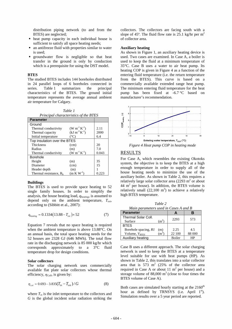
collectors. The collectors are facing south with a slope of 45º. The fluid flow rate is 25.1 kg/hr per m2 of collector area. Auxiliary heating As shown in Figure 1, an auxiliary heating device is used. Two cases are examined. In Case A, a boiler is used to keep the fluid at a minimum temperature of 35°C. Case B uses a water to air heat pump. Its heating COP is given in Figure 4 as a function of the entering fluid temperature (i.e. the return temperature from the BTES). This curve is based on a commercially available extended range heat pump. The minimum entering fluid temperature for the heat pump has been fixed at -6.7 °C based on manufacturer’s recommendation.

Figure 4 Heat pump COP in heating mode

RESULTS For Case A, which resembles the existing Okotoks system, the objective is to keep the BTES at a high enough temperature in order to supply all of the house heating needs to minimize the use of the auxiliary boiler. As shown in Table 2, this requires a relatively large solar collector area (2293 m2 or about 44 m2 per house). In addition, the BTES volume is relatively small (22,100 m3) to achieve a relatively high BTES temperature.

Table 2 Main parameters used in Cases A and B

Parameter A B Thermal Solar Coll. Surface (m2)

2293 573

BTES Borehole spacing, R1 (m) Volume, VBTES (m3)

2.25

22 100

4.5

88 000 Auxiliary heating Boiler HP

Case B uses a different approach. The solar charging network is used to keep the BTES at a temperature level suitable for use with heat pumps (HP). As shown in Table 2, this translates into a solar collector area that is 573 m2 (25% of the collector area required in Case A or about 11 m2 per house) and a storage volume of 88,000 m3 (close to four times the BTES volume of Case A). Both cases are simulated hourly starting at the 2160th hour as defined by TRNSYS (i.e. April 1st). Simulation results over a 5 year period are reported.

- 604 -

Figure 5 BTES temperatures for Cases A and B over 5 years

Figure 5 shows the evolution of the average BTES temperature over the simulation period for Cases A and B. The first thing to note in Figure 5 is that the average BTES temperature reaches a quasi steady-state behaviour after 5 years with small temperature variations from year to year for both cases. During the fifth year, the average BTES temperature ranges from about 44°C to a little over 70°C. However, in the winter, local temperatures near the boreholes (not shown in Figure 5) are below 35°C, the minimum temperature required for space heating. For Case B, the BTES average temperature ranges from 10 to 16oC during the fifth year, thus slightly above the annual mean ambient temperature. The entering fluid temperature to the heat pump (not shown in Figure 5) varies from -5.5°C to 21°C. Note that for both cases, the results presented in Figure 5 are similar to those obtained in an earlier study (Chapuis and Bernier, 2008) with a different approach to model the counter-current borehole heat exchanger. For the 5th year of operation, the monthly energy flows for Cases A and B are shown respectively in Figure 6 and 7 and an annual results summary for the two cases is presented in Table 3.

Figure 6 - Case A - 5th year energy flows

As expected in case A, solar energy collection peaks in the summer (close to 125 MWh in July) and the heating load is maximum (also near 125 MWh) in December. Since the BTES is at a relatively high temperature, heat losses are significant, particularly in the summer months. On a annual basis, the BTES heat losses (312 MWh) represent 33% of a the total collected solar energy. The average yearly solar collector efficiency is 23%. This value is relatively low and is due to the high temperature level achieved in the BTES. As indicated in Figure 6, auxiliary heating is required in February and March. This is due to the fact that the exit fluid temperature is lower than the minimum required for space heating (35°C). However, the total amount of auxiliary heating required is small at 11 MWh. Thus, on an annual basis, solar energy supplies 98% of the space heating needs.

Table 3 5th year – Annual results summary

Result from simulation A B Solar coll. efficiency (-) 0.23 0.58 Solar collected energy (MWh) 946 598 Heat pump compressor (MWh) - 144 Auxiliary boiler (MWh) 11 - BTES thermal losses (MWh) 312 82 Solar fraction (-) 0.98 0.78

In case B, the thermal losses are relatively small at 82 MWh due to low BTES temperatures (Figure 5). They represent 14% of the total amount of solar energy collected. This value is much lower than in Case A. The average solar collector efficiency is relatively high at 58%. Finally, the amount of energy input to the heat pump compressor is 144 MWh which represents 22% of the space heating needs. In other words, the solar-BTES system supplies 78% of the space heating needs during the 5th year.

Figure 7 - Case B - 5th year energy flows

- 605 -

Figure 8 shows the energy flows and temperature level for a particular hour where there is simultaneous charging and discharging for Case B. In this particular case, there is 333 kW of solar energy incident on the solar collector. Out of this amount, 210 kW is transferred to the BTES. On the discharge side, the space heating requirements are 30 kW. This load is met using 24 kW of stored energy in the BTES and 6 kW of compressor power. Finally, the BTES losses heat at a rate of 2.03 kW for that particular hour.

Figure 8 – Case B - Energy flows 20579th hour, Text=9.6°C

CONCLUSION A novel counter-current borehole heat exchanger model using two independent U-tube networks has been implemented in TRNSYS. The original DST model (type 557a of the TESS libraries) has been modified to handle simultaneous charging and discharging in the same borehole. The first part of the paper is devoted to a thorough description of the original DST model followed by details on the modifications made to handle the two independent circuits. In the second part of the paper, the modified DST model is used to model a BTES system linked to solar collectors on the charging side and to a series of 52 homes on the discharge side. Hourly simulations over a period of 5 year are reported for the Calgary (Alberta, Canada) climate. Results show that it is possible to have a solar fraction of 98% for space heating with 2293 m2 of flat plate solar collectors. However, in order to accomplish such a high solar fraction, the BTES temperature has to be kept relatively high. This leads to BTES losses which represent 33% of the collected solar energy and to relatively small solar collector efficiency (23%). In a second scenario, the solar collector area is reduced by a factor of 4 accompanied with a four fold increase of the BTES volume. With this configuration, BTES thermal losses are reduced but the BTES temperature is too low to provide direct space heating. However, by using a heat pump, this temperature level can be increased for space heating. With this scenario, the solar fraction reaches 78% with an average solar collector efficiency of 58%.

NOMENCLATURE

pc Ground vol. specific heat [kJ m -3 K-1]

fC Fluid volumetric specific heat [kJ m -3 K-1]

H Borehole height [m]

totNBH Total number of boreholes [-]

qheating House heating load [kW]

fQ Fluid flow vol. [m3 s-1]

bR Borehole thermal resistance [m K W-1]

,2LocR Thermal resistance between the

fluid and the midpoint of Local mesh no.2 [m K W-1]

,2Locr Inner radius of Local mesh no.2 [m]

,2Locr Midpoint radius of Local mesh

no.2 [m]

bT Temperature at borehole wall [°C]

,2LocT Temperature of Local mesh no.2 [°C]

V Volume [m3] Ground thermal diffusivity [m2 s-1] Ground thermal conductivity [W m-1 K-1]

REFERENCES

Chapuis, S., Bernier, M. 2008. Étude préliminaire sur le stockage solaire saisonnier par puits géothermiques. Proceedings of the 3rd Canadian Solar Buildings Conference, Fredericton (N.-B.), Canada, pp. 14-23.

Claesson, Eftring, Hellström, Johansson. 1981. Duct storage model, Dept. of mathematical physics, Lund institute of technology, Sweden.

Hellström, G., 1991. Ground Heat Storage – Thermal Analyses of Duct Storage Systems- I. Theory, Dept. of Mathematical Physics, Univ. of Lund, Sweden.

Hellström, G., 1989. Duct Ground Heat Storage Model: Manual for Computer Code, Dept. of Mathematical Physics, Univ. of Lund, Sweden.

Klein, S. A., et al. 2004. TRNSYS 16 – A TRaNsient SYstem Simulation program, Solar Energy Laboratory. Univ. of Wisconsin. USA.

Mazzarella, L., 1989. Duct storage model for TRNSYS 1989 version, ITW, Stuttgart Univ., Dipartimento di Energetica, Politechnico di Milano, Italy.

McDowell, T.P., Thornton J.W. 2008. Simulation and model calibration of a large-scale solar seasonal storage system, 3rd National conference of IBPSA-USA, Berkeley (California), USA.

Pahud.D, 1996. Duct storage model for TRNSYS 1996 version, LASEN-EPFL, Lausanne, Switzerland.

Pitts, D., Sissom, L. 1997. Heat Transfer, 2nd Edition, Schaum’s Outlines Series, McGraw-Hill, NY, USA.

Sibbitt, B., Onno, T., McClenahan, D., Thornton, J., Brunger, A., Kokko J., Wong. B. 2007. The Drake Landing Solar Community Project – Early Results, 2nd Canadian Solar Buildings Conference, Calgary (Alberta), Canada.

TESS, 2004. TESS Libraries V. 2, User manual. Thermal Energy Systems Specialists, Madison, WI, USA.

- 606 -