Searching and Sorting

Search

One of the most common problems for an algorithm to solve is to search for some data in some data structure.

We will discuss the (time) complexity of search in

• a list

• a binary search tree

Simplifying assumptions

• Search can be defined so long as the underlying data type is in Eq. But (==) might be an expensive operation• However this is not relevant for the complexity analysis of the ad hoc

polymorphic search algorithm on its own

• We assume that the data structure we are searching in is completely computed before we start searching• Not necessarily true due to laziness, but again, not relevant to the search

algorithm on its own

Search in a list

elem :: Eq a => a -> [a] -> Bool

elem x list = case list of

[] -> False

y:ys | x == y -> True

| otherwise -> elem x ys

(This is not identical to the definition of elem in the Prelude, but it gives the idea)

Best case analysis

Given a finite list of length n, what is the best case scenario for elem?• We can assume n is large, and so not empty

Best case – the searched-for element is the head of the list

• Check if the list is empty

• Check if its main constructor is cons

• Check if x == y

• Return True

Best case analysis

These operations take time• maybe a lot of time if (x == y) is expensive

But the time does not depend on the length of the list.

Therefore in the best case elem is constant – O(1)

Worst case analysis

The worst case – the searched-for element is not in the list at all

• n+1 checks if the list is empty

• n checks if main constructor is cons

• n checks if x == y

• n recursive calls

• Return False

Worst case analysis

Remember that anything that increases as the input size increases will eventually dominate anything that is constant, so remove all constants

• n+1 checks if the list is empty

• n checks if main constructor is cons

• n checks if x == y

• n recursive calls

• Return False

Worst case analysis

Remember that anything that increases as the input size increases will eventually dominate anything that is constant, so remove all constants

• O(n) checks if the list is empty

• n checks if main constructor is cons

• n checks if x == y

• n recursive calls

Worst case analysis

The function describing the time spent searching the list will then be

n * (cost of empty check + cost of cons check + cost of (==) + cost of recursive call) + some constant

But complexity analysis asks us to ignore constants, whether they are multiplied or added, so…

In the worst case, elem is linear – O(n).

Note that the case where the element is at the end of the list is also O(n).

Average case analysis

Average cases can be tricky – on average, how likely is it that an element will be in a list?

But across the cases that the element is in the list, we can obviously define an average case – where the element is halfway through.

But if searching the whole list takes time O(n), then searching half a list takes time proportional to n/2 – and this is also O(n)

Search in a binary search tree

Data BSTree a = Null | Node (BSTree a) a (BSTree a)

BSElem :: Ord a => a -> BSTree a -> Bool

BSElem x tree = case tree of

Null -> False

Node left node right

| x < node -> BSElem x left

| x == node -> True

| otherwise -> BSElem x right

Search in a binary search tree

In the best case, we are again in O(1). What about worst case?

Simplifying assumptions:

• The BSTree really is a binary search tree – all operations on it have kept it correctly ordered

• The tree is balanced – Node Null 1 (Node Null 2 (Node Null 3 (Node Null 4)))

is technically a BSTree, but it is not any faster to search than a list!

Logarithms

Logarithms are the inverse of exponentiation:

If bc = a then logba = c

• log21 = 0 because 20 = 1

• Log22 = 1 because 21 = 2

• log24 = 2 because 22 = 4

• log28 = 3 because 23 = 8

• log216 = 4 …

Height of a binary search tree

In a balanced BStree the height h as a function of its size n is approximately

h = log2(n + 1)

e.g. a tree of height 4 contains (at most) 15 elements.

We can ignore the ‘+1’, and, for large n, log2n will dominate the number of any missing elements at the bottom layer.

In fact the base 2 is also irrelevant for big O analysis – we can say that his in O(log n).

Worst and average case analyses of BSElem

In the worst case BSElem looks at one element for every layer of the tree, so it is in O(log n).

The average height of an element in a tree can be approximated as log2(n-1), so the average case analysis for search is again O(log n).

Comparison

n log2n multiplier2 1 2

16 4 4128 7 18

1,024 10 1028,192 13 630

65,536 16 4,096524,288 19 27,594

Sorting

Data that is unorganised is a pain to use

It is hence important to know how to sort (put things in order)

We will look at sorting lists, with a focus on complexity

Insertion Sort

Problem: sort a list of numbers into ascending order.

Given a list [7,3,9,2]

1. Suppose the tail is sorted somehow to get [2,3,9]

2. Insert the head element 7 at the proper position in the sorted tail to get [2,3,7,9]

The tail is sorted ‘somehow’ by recursion, of course!

Insertion

insert :: Ord a => a -> [a] -> [a]

insert x list = case list of

[] -> [x]

y:ys

| x <= y -> x : y : ys

| otherwise -> y : insert x ys

If the input list is sorted, the output list will be also

Complexity of Insertion

Best case: compare only to the head and insert immediately – O(1)

Worst case: look through the whole list and insert at the end – O(n)

Average case: insert after half the list – O(n)

Insertion Sort

iSort :: Ord a => [a] -> [a]

iSort = foldr insert []

Make sure that you understand this definition• What are the types of its components?• What does it do on the base case?• What does it do on the step case?

Most importantly, halfway through the algorithm, which part of the list is sorted, and which is not?

Complexity of Insertion Sort

Best case: the list is already sorted, so each element is put onto the head of the list immediately – O(n)

Worst case: the list is sorted in reverse order!

Each element needs to be compared to the tail of the list.

What is the cost of this?

Worst Case Complexity of Insertion Sort

Say sorting the last element of the list takes 1 step

Then sorting the next element takes 2 steps, and so on, with n steps for the first element of the list

So we have the sum 1 + 2 + 3 + … + (n-2) + (n-1) + n

= (n/2) * (n + 1)

Delete the constants and dominated parts of the expression…

= O(n2)

Average Case Complexity of Insertion Sort

The average case complexity of insert was the same (with respect to big-O notation) as the worst case.

So we again have 1 + 2 + 3 + … + (n-2) + (n-1) + n

= O(n2)

Merge Sort

Merge Sort is a ‘divide and conquer’ algorithm.

Intuition: sorting a list is hard…

But sorting a list of half the size would be easier (Divide)

But it is easy to combine two sorted lists into one sorted list (Conquer)

Merge

merge :: Ord a => [a] -> [a] -> [a]merge list1 list2 = case (list1,list2) of(list,[]) -> list([],list) -> list(x:xs,y:ys)

| x <= y -> x : merge xs (y:ys)| otherwise -> y : merge (x:xs) ys

If we have two lists sorted somehow, their merge is also sortedSomehow = recursion, again!

Complexity of Merge

Assuming that the two lists are of equal length, let n be the list of the two combined.

Best case: one list contains elements all smaller than the other. Only need roughly n/2 comparisons – O(n)

Worst case: Every element gets looked at, but we are always ‘dealing with’ one element per step – O(n)

Average case: Where best case = worst case, this is obvious!

Merge Sort

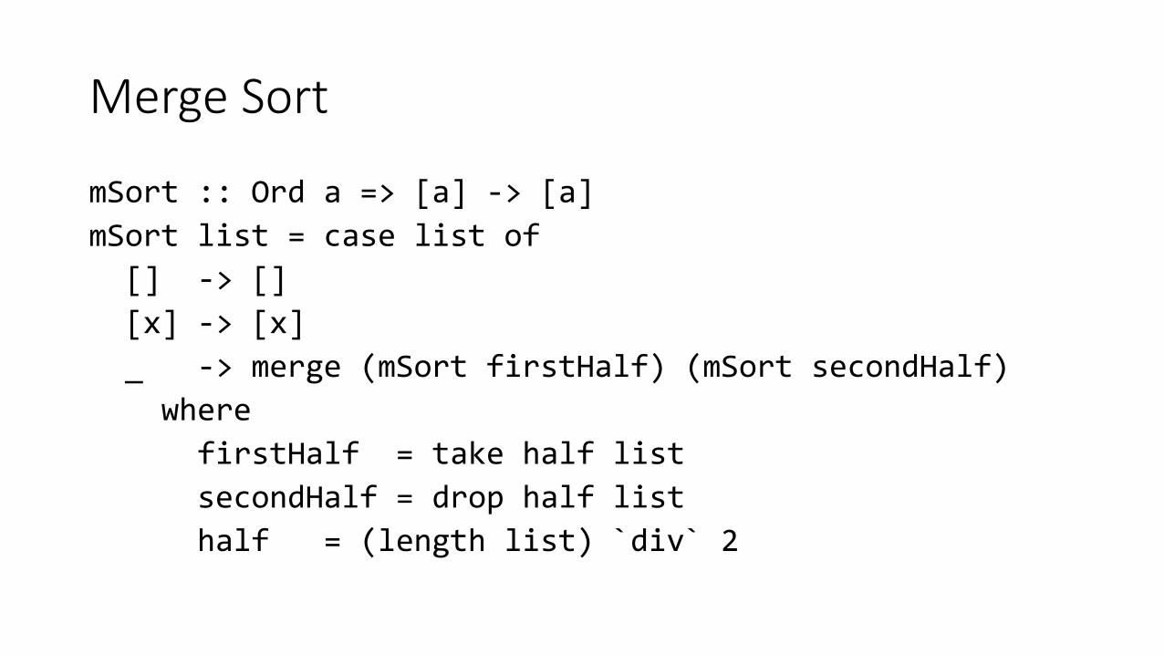
mSort :: Ord a => [a] -> [a]

mSort list = case list of

[] -> []

[x] -> [x]

_ -> merge (mSort firstHalf) (mSort secondHalf)

where

firstHalf = take half list

secondHalf = drop half list

half = (length list) `div` 2

Complexity of Merge Sort

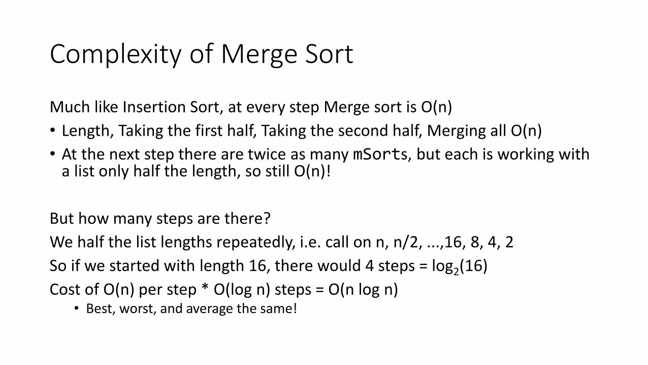
Much like Insertion Sort, at every step Merge sort is O(n)

• Length, Taking the first half, Taking the second half, Merging all O(n)

• At the next step there are twice as many mSorts, but each is working with a list only half the length, so still O(n)!

But how many steps are there?

We half the list lengths repeatedly, i.e. call on n, n/2, ...,16, 8, 4, 2

So if we started with length 16, there would 4 steps = log2(16)

Cost of O(n) per step * O(log n) steps = O(n log n)• Best, worst, and average the same!

Comparison

n n log2n n2 multiplier2 2 4 2

16 64 256 4128 896 16,384 18

1,024 10,240 1,048,576 1028,192 106,496 67,108,864 630

65,536 1,048,576 4,294,967,296 4,096

Comparison of Sorting Algorithms

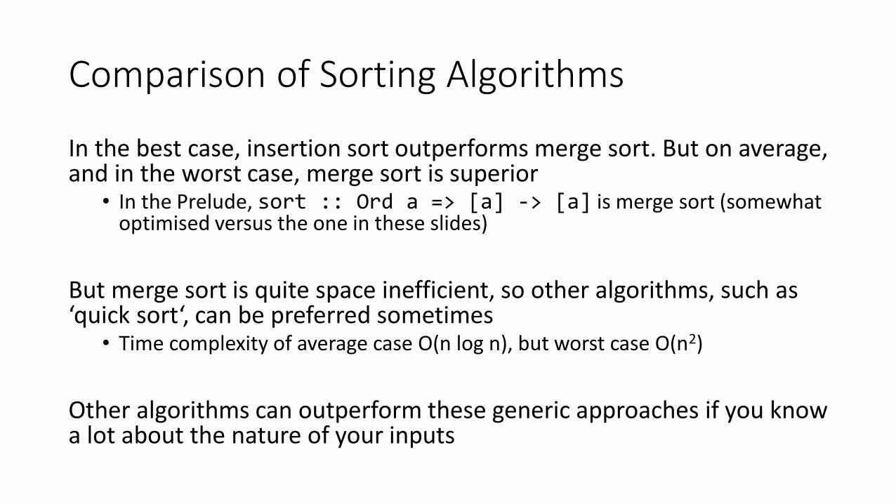
In the best case, insertion sort outperforms merge sort. But on average, and in the worst case, merge sort is superior

• In the Prelude, sort :: Ord a => [a] -> [a] is merge sort (somewhat optimised versus the one in these slides)

But merge sort is quite space inefficient, so other algorithms, such as ‘quick sort‘, can be preferred sometimes

• Time complexity of average case O(n log n), but worst case O(n2)

Other algorithms can outperform these generic approaches if you know a lot about the nature of your inputs