search in mixed-integer linear...
TRANSCRIPT

JOHN W. CHINNECKS Y S T E M S A N D C O M P U T E R E N G I N E E R I N G
C A R L E T O N U N I V E R S I T Y
O T T A W A , C A N A D A
Search in Mixed-Integer Linear Programming

B R A N C H A N D B O U N D B A S I C S
W H A T I S M I X E D - I N T E G E R P R O G R A M M I N G ( M I P ) ?
B R A N C H A N D B O U N D F O R M I P
O B S E R V A T I O N S
I. Fundamentals2
Chinneck: Search in MIP

Branch and Bound Basics
Application: searching a discrete space
Node: represents subsets of possible solutions.
Branch: generate child nodes from current node.
3
Chinneck: Search in MIP
Root node
Leaf nodes
AH Land, A Doig (1960). An Automatic Method of Solving Discrete Programming Problems, Econometrica 28.

The Bounding Function
Chinneck: Search in MIP
4
Bound: optimistic bound on the best possible solution at descendent of current node.
As accurate as possible, but... Underestimate for minimization; Overestimate for maximization
Incumbent: best complete feasible solution yet found. Updated as solution proceeds.
Prune: remove node under certain conditions Descendent cannot be optimum: bounding function value worse
than incumbent objective function value. Node and descendents cannot be feasible: decisions thus far
prevent one or more constraints from ever being satisfied.
Stop: when incumbent objective function value is better than (or equal to) the best bound on any node.
Optimistic bounding function guarantees optimality. “Better than or equal to” finds alternative optima

What is Mixed-Integer Programming?
Chinneck: Search in MIP
5
Linear objective function (Z) and constraints
Variables: continuous / integer / binary At least one integer or binary variable
Hereafter: “integer” includes “binary”
MILP (or MIP) includes: Mixed problems (at least one continuous variable)
Pure integer problems
Pure binary problems
Integer variables make it a discrete search problem
Goal: best solution that also satisfies all integralityconditions

Branch and Bound for MIP
Chinneck: Search in MIP
6
Bounding function at a node: linear program (LP) solution ignoring integer restrictions.
Called the LP-relaxation.
Integer-feasible solution: All integer variables have integer values.
Leaf nodes are either: Integer-feasible (no descendent will be better)
Infeasible (and no descendent will be feasible)
Intermediate node: solution satisfies all linear constraints and bounds (original or
added), but not all integrality constraints.
Designing a MIP B&B Algorithm
Chinneck: Search in MIP
7
3 major search rule design decisions: Branching variable selection Branching direction selection Node selection: which node to explore next?
Numerous other heuristics: Local search Root node heuristics Etc.
MIP: B&B framework (guarantees optimum), plus numerous heuristics

Branching Variable and Direction Selection
Chinneck: Search in MIP
8
Candidate variable: integer variable having non-integer value in current LP relaxation solution.
E.g. x3 =5.7 in LP solution. Branching on x3 creates two child nodes:
Down branch: parent LP + revised bound x3 ≤ 5
Up branch: parent LP + revised bound x3 ≥ 6
Search design issues:
How to choose the branching variable?
How to choose the branching direction (up or down)?
The other child node may be visited later...

Branching on a Variable
Chinneck: Search in MIP
9
LP at parent node Branch on x1:
two child node LPs
x1 integer in child solns
Z(3.75, 2.25) = 41.25x1 ≥ 4
x1 ≤ 3
Down child
Up child
x1
x2

Node Selection
Chinneck: Search in MIP
10
Search issue: which node to explore next?
Depth-first:
Choose next node from among last nodes created
Common choice for MIP
Big advantage:
Next LP identical to last one solved, except for one bound
Next solution very quick due to advanced LP start
Many other options (more later...)

Simple Example
Chinneck: Search in MIP
11
Maximize Z = 8x1 + 5x2
s.t. x1 + x2 6
9x1 + 5x2 45
x1, x2 are integer and nonnegative
Search rules:
Node selection: depth first. Simple backtrack at leaf.
Branching variable selection: natural order.
Branching direction: down.

1. Root Node
Chinneck: Search in MIP
12
Root node LP solution: Z(3.75, 2.25)=41.25
Both variables are candidates: choose x1, branch down.
Z(3.75,2.25) = 41.25

2. Add Bound: x1 ≤ 3
Chinneck: Search in MIP
13
Integer-feasible!
First incumbent: Z(3,3)=39
Still active nodes with bound > incumbent so continue.
Next: backtrack and branch on x1, up.
Z(3,3) = 39
added bound x1 ≤ 31. Root nodeZ(3.75,2.25)=41.25
2. Z(3,3)=39
add x1≤3

3. Add bound: x1 ≥ 4
Chinneck: Search in MIP
14
Not integer-feasible, bound > incumbent.
Still active nodes with bound > incumbent so continue.
Next: continue depth-first, branch on x2, down.
Z(4,1.8)=41
added bound x1≥4
1. Root nodeZ(3.75,2.25)=41.25
2. Z(3,3)=39
add x1≤3
3. Z(4,1.8)=41
add x1≥4
4. Branch Down on x2
Chinneck: Search in MIP
15
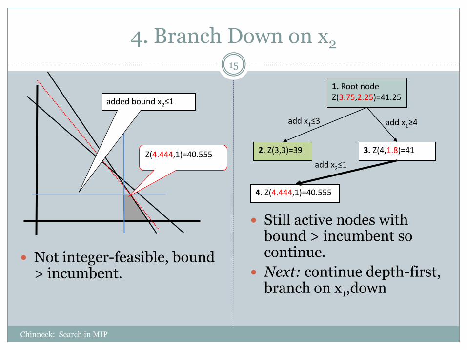
Not integer-feasible, bound > incumbent.
Still active nodes with bound > incumbent so continue.
Next: continue depth-first, branch on x1,down
Z(4.444,1)=40.555
added bound x2≤1
1. Root nodeZ(3.75,2.25)=41.25
2. Z(3,3)=39
add x1≤3
3. Z(4,1.8)=41
add x1≥4
4. Z(4.444,1)=40.555
add x2≤1

5. Branch Down on x1
Chinneck: Search in MIP
16
Integer-feasible, but worse than incumbent: prune.
Still active nodes with bound > incumbent so continue.
Next: backtrack, branch on x1, up.
Z(4,1)=37
added bound x1≤4 Note: x1≥4 added previously
feasible
1. Root nodeZ(3.75,2.25)=41.25
2. Z(3,3)=39
add x1≤3
3. Z(4,1.8)=41
add x1≥4
4. Z(4.444,1)=40.555
add x2≤1
5. Z(4,1)=37
add x1≤4

6. Backtrack, add x1≥5
Chinneck: Search in MIP
17
Feasible, replaces incumbent. Still active nodes with bound > incumbent so continue.
Next: backtrack, branch on x2, up.
Z(5,0)=40
single feasible point
added bound x1≥5
1. Root nodeZ(3.75,2.25)=41.25
2. Z(3,3)=39
add x1≤3
3. Z(4,1.8)=41
add x1≥4
4. Z(4.444,1)=40.555
add x2≤1
5. Z(4,1)=37
add x1≤4
6. Z(5,0)=40
add x1≥5

7. Backtrack, Add x2≥2
Chinneck: Search in MIP
18
Infeasible! Nowhere to backtrack: exit.
Solution: Z(5,0)=40.
added bound x2≥2
1. Root nodeZ(3.75,2.25)=41.25
2. Z(3,3)=39
add x1≤3
3. Z(4,1.8)=41
add x1≥4
4. Z(4.444,1)=40.555
add x2≤1
5. Z(4,1)=37
add x1≤4
6. Z(5,0)=40
add x1≥5
7. Infeasible
add x2≥2

General B&B Algorithm for MIP
Chinneck: Search in MIP
19
N: list of unexplored nodes, initially empty. No incumbent at start.1. Solve root node LP relaxation. Add it to N.2. Choose node from N for exploration.3. Solve LP relaxation for current node.
If LP solution infeasible: go to Step 7. If LP solution is integer-feasible:
Worse than incumbent, then go to Step 7. Better than incumbent, replace it, go to Step 7.
4. Choose candidate variable in current node for exploration.5. Create two child nodes using branching variable, add to N.6. Go to Step 2.7. If N is empty then:
1. If no incumbent, exit with infeasible outcome.2. Else exit with incumbent as optimum solution.
8. Go to Step 2.

Observations: Squaring-off
Chinneck: Search in MIP
20
Adding bounds “squares off” the feasible region
Objective function eventually “catches” on a squared-off cornerpoint
Number of candidates generally decreases deeper in tree

Depth and Bounding Function Value
Chinneck: Search in MIP
21
Bounding function values get worse (or stay the same) as you descend
Each new level removes part of parent feasible region: LP relaxation solution can
only get worse (or stay the same)
Solution stalls when bounds do not change much between levels
1. Root nodeZ(3.75,2.25)=41.25
2. Z(3,3)=39
add x1≤3
3. Z(4,1.8)=41
add x1≥4
4. Z(4.444,1)=40.555
add x2≤1
5. Z(4,1)=37
add x1≤4
6. Z(5,0)=40
add x1≥5
7. Infeasible
add x2≥2

Observations
Chinneck: Search in MIP
22
Any set of tree rules (node selection, branching variable selection and direction) will solve the MIP correctly. Different sets of rules generate different trees Some trees are much more efficient!
Simplex method preferred for LP solutions because of ease of advanced start in child nodes.
Some MIPs do not terminate (rare).
Good early incumbent helps prune the search tree. Nodes with worse values of bounding function are removed.

Converging Bounds
Chinneck: Search in MIP
23
MIP solved when the upper and lower bounds converge: incumbent objective
function value
best bounding function value
To speed the process: Better incumbents
early
Tighter bounding function values
Incumbent objective functionvalue
Best bounding function value
Nodes explored
Converging bounds when minimizing

Measuring Solution Speed
Chinneck: Search in MIP
24
Total solution time: the gold standard.
Total simplex iterations Approximates total time
Ignores non-LP time (e.g. choosing node, variable, etc.)
Useful if running on heterogeneous machines
Total number of nodes May not correlate with time at all
E.g. Depth-first search may have many more nodes but take much less time due to simplex advanced starts.
Example: pk1 Depth-first: 4058 s; 9,778,734 iterations; 1,965,503 nodes
Best-projection: 12,623 s; 4,329,434 iterations; 820,924 nodes

N O D E S E L E C T I O N
B R A N C H I N G V A R I A B L E S E L E C T I O N
B R A N C H I N G D I R E C T I O N S E L E C T I O N
O T H E R C O N C E P T S
Chinneck: Search in MIP
25
State of the Art

Node Selection
Chinneck: Search in MIP
26
General goal (unrealistic): always choose a node that is an ancestor of an optimum node.
i.e. Avoid superfluous search
How much difference does it make?
Mas76: depth-first 1,307 s, best-projection 20,610 s
Philosophies:
Pattern-based: breadth-first, depth-first
Forecasting: best-first, best-estimate, best-projection

Depth-First Node Selection
Chinneck: Search in MIP
27
Choose next node from among last nodes created
Also need rule for branching direction: branch up or down?
Backtrack at leaf node:
Choose last created active node.
Speed advantage for MIP:
Next LP identical to last one solved, except for one bound
Next solution very quick due to advanced LP start
Often finds first incumbent early

Breadth-First Node Selection
Chinneck: Search in MIP
28
Add nodes to bottom of a list as they are created
Choose next node from top of list
1
2 3
4 5 6 7 8
9 10

Best-First Node Selection
Chinneck: Search in MIP
29
Forecasting method, but with limited lookahead Just a bound on how well you might do
Choose unexplored node with best bounding function value anywhere in tree Unexplored nodes initially given bounding function value from
parent node.
Disadvantage for MIP: Frequent re-starts of simplex solution without having the
factorized basis from the parent node.

Best-Projection Node Selection
Chinneck: Search in MIP
30
Forecasting, with lookahead:
Project objective function value at a feasible descendent of current node.
Assume constant rate of worsening of Z per unit integer infeasibility at the root node solution.
For minimization, Zincumbent > Zroot:
For min: choose node that gives smallest estimate.
i
root
rootincumbentii Inf
Inf
ZZZestimate

An Aside: Pseudo-Costs
Chinneck: Search in MIP
31
Estimate effect on Z due to change in value of variable
Minimizing: Zchild ≥ Zparent , so Z = Zchild– Zparent
fj = fractional part of variable, e.g. 0.7 if x =9.7
Calculate separately for up and down branches on every integer variable,
Many different estimating and updating schemes
)1/(
/
j
up
j
up
j
j
down
j
down
j
fZP
fZP

Best-Estimate Node Selection
Chinneck: Search in MIP
32
Forecasting, with lookahead based on pseudo-costs Estimate Z at a feasible descendent of current node using pseudo-
costs for each candidate variable
For minimization:
j j
up
jj
down
jii fPfPZestimate )1(,min

Other Node Selection Variants
Chinneck: Search in MIP
33
Most feasible node selection: choose node having smallest sum of fractional values over all candidate variables
Combinations:
Depth-first to first incumbent, then best-first
Interleave best-estimate with occasional best-first
Etc.

Triggering Backtrack or Jumpback
Chinneck: Search in MIP
34
Assuming depth-first node selection:backtrack at a leaf (LP-infeasible or integer-feasible)
Any other reasons to backtrack or jumpback?
Jumpback: select a node other than the backtrack node
Trigger using aspiration value:
User-selected limit on objective function value:
Bounding function value must be at least this good to explore node
Backtrack or jumpback if node bound is worse than the aspiration value

Branching Variable Selection
Chinneck: Search in MIP
35
How much difference does it make?
Momentum1: time to first incumbent
Cplex 9.0 default: time out at 28,800 s. Method B: 75 s.
Most common idea:
Choose variable that worsens Z the most in child node
Gives a tighter bound on descendent nodes
Some methods choose variable and direction

Simple Variable Selection
Chinneck: Search in MIP
36
Choose variable that is closest to feasibility
Choose variable that is farthest from feasibility (closest to fj = 0.5)

Pseudo-Cost Variable Selection
Chinneck: Search in MIP
37
Choose variable whose pseudo-cost worsens Z the mostin one of the child nodes:
Maxj{Pjup×(1-fj), Pj
down×fj}
Alternatively choose variable that has:
Maximum sum of degradations: Maxj{Pj
up×(1-fj) + Pjdown×fj}
Maximum minimum degradation:Maxj{min(Pj
up×(1-fj), Pjdown×fj)}
Maximum product of degradations:Maxj{Pj
up×(1-fj) × Pjdown×fj}

Strong Branching and Variants
Chinneck: Search in MIP
38
Full strong branching:
Solve LP for up and down direction for every candidate varb.
Choose variable and direction that degrade Z the most
Computationally very expensive!
Approximations to full strong branching:
Limit the number of simplex iterations in each LP
Limit which candidate variables are tested (e.g. based on pseudo-costs)

Driebeek and Tomlin
Chinneck: Search in MIP
39
1. Approximate strong branching:
Just one dual simplex pivot for each LP[can actually just be estimated, not performed]
2. Choose variable that has largest degradation in either direction
3. Choose direction that gives smallest degradation
Default branching method in GLPK

Many Variants:
Chinneck: Search in MIP
40
Hybrid strong/pseudo-cost branching
Strong branching high in tree
Pseudo-cost branching below a certain level
Reliability branching:
Pseudo-cost branching, except...
Strong branching on varbs with uninitialized pseudo-costs and unreliable pseudo-costs
Etc.
Branching Direction Selection
Chinneck: Search in MIP
41
Common rules:
Branch up always
Generally best in practice.
Branch down always
Branch to closest bound
Branch to farthest bound
Direction that forces branching variable away from its value at the root node
Solver-proprietary rules
Other Concepts
Chinneck: Search in MIP
42
Branch and Cut Branch and Price Preprocessing and Probing Neighbourhood search:
Limited B&B search in the “neighbourhood” of promising node
Special Ordered Sets: Enforce specified order of variable selection under certain conditions
Specialized feasibility-seeking algorithms: OCTANE for binary problems Pivot-and-complement, pivot-and-shift The feasibility pump prior to B&B
No-good learning General disjunctions:
Linear disjunctions that are not axis-parallel
Parallel processing Etc.!

A C T I V E - C O N S T R A I N T V A R I A B L E S E L E C T I O N
N E W N O D E S E L E C T I O N M E T H O D S
B R A N C H I N G T O F O R C E C H A N G E
G E N E R A L D I S J U N C T I O N S
Chinneck: Search in MIP
43
New Directions

Active-Constraint Variable Selection
Chinneck: Search in MIP
44
Concept:
LP-relaxation optimum is fixed by active constraints
For different child optima, must impact the active constraints
Choose candidate variable that has most impact on active constraints in current LP-relaxation solution
Constraint-oriented approach vs. usual objective-function-oriented approaches
Focus on reaching first incumbent quickly

Illustration
Chinneck: Search in MIP
45
y
x
LP relaxation before branching
Branch on x Branch on y
Feasible Region

Estimating Impact on Active Constraints
Chinneck: Search in MIP
46
1. Calculate “weight” Wik of each candidate i in each active constraint k
0 if the candidate does not appear in constraint
2. For each candidate, total the weights over all of the active constraints.
3. Choose candidate having largest total weight.
Dynamic variable ordering: changes at each node
Many variants: A through P

Overview of Weighting Methods
Chinneck: Search in MIP
47
Is candidate variable in active constraint or not?
Relative importance of active constraint: Smaller weight if more candidate or integer variables: changes in
other variables can compensate for changes in selected variable.
Normalize by absolute sum of coefficients.
Relative importance of candidate variable within active constraint: Greater weight if coefficient size is larger: candidate variable has
more impact.
Sum weights over all active constraints? Look at biggest impact on single constraint?
Etc.

Some of the Better Weighting Schemes
Chinneck: Search in MIP
48
A: Wik=1.
B: Wik = 1/ [Σ(|coeff of all variables|].
L: Wik = 1/(no. integer variables)
O: Wik = |coeffi|/(no. of integer variables)
P: Wik = |coeffi|/(no. of candidate variables)
H methods: choose largest individual value of Wik
HM: Wik = 1/[no. candidate variables]
HO: Wik = |coeffi|/(no. of integer variables)
Variants: voting, multiply by dual costs, etc.

Test Models
Chinneck: Search in MIP
49
MIPLIB 2003 set
60 models (58 used: 2 time out on all methods)
Range of difficulties
Rows: 6–159,488
Variables: 62–204,880
Integer variables: 1–3,303
Binary variables: 18–204,880
Continuous variables: 1–13,321
Nonzeroes: 312–1,024,059
Experiments
Chinneck: Search in MIP
50
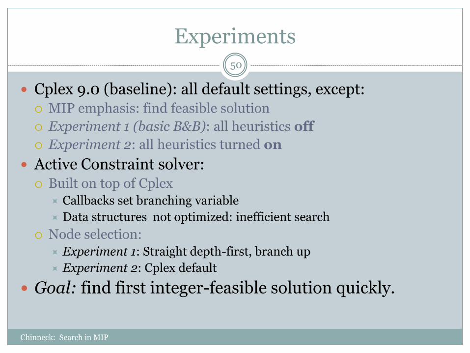
Cplex 9.0 (baseline): all default settings, except: MIP emphasis: find feasible solution
Experiment 1 (basic B&B): all heuristics off
Experiment 2: all heuristics turned on
Active Constraint solver: Built on top of Cplex
Callbacks set branching variable
Data structures not optimized: inefficient search
Node selection:
Experiment 1: Straight depth-first, branch up
Experiment 2: Cplex default
Goal: find first integer-feasible solution quickly.
Experiment 1: Heuristics Off
Chinneck: Search in MIP
51
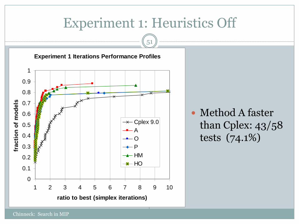
Method A faster than Cplex: 43/58 tests (74.1%)
Experiment 1 Iterations Performance Profiles
0
0.1
0.2
0.3
0.4
0.5
0.6
0.7
0.8
0.9
1
1 2 3 4 5 6 7 8 9 10
ratio to best (simplex iterations)
fracti
on
of
mo
dels
Cplex 9.0
A
O
P
HM
HO

Experiment 2: Heuristics On
Chinneck: Search in MIP
52
25 models used: 32 solved at root node
3 failed on all methods
Method B faster than Cplex: 14/25 models (56%)
Cplex heuristics on: Half of models solve
faster than before
Half of models solve slower than before
Experiment 2 Iterations Performance Profiles
0
0.1
0.2
0.3
0.4
0.5
0.6
0.7
0.8
0.9
1
1 2 3 4 5 6 7 8 9 10
ratio to best (iterations)
fracti
on
of
mo
dels
Cplex 9.0
B
L
P
HM
HO

First Incumbent Better than Cplex
Chinneck: Search in MIP
53
Optimality Gap measures “distance” of solution from (unknown) optimum solution
For minimization: Zlow: lowest bound on an active node
Optimality gap: [|Zlow – Zincumbent|]/[ε+|Zlow|]
Experimental Results: Exp. 1: active constraint methods have smaller gaps than Cplex
(53% for A, 78% for method P)
Exp. 2: active constraint methods have smaller gaps than Cplex(75% for B, 50% for HM)

New Node Selection Methods
Chinneck: Search in MIP
54
Triggering Backtrack Feasibility Depth ExtrapolationModified Best Projection Aspiration
Choosing Node When BacktrackingModified Best ProjectionDistribution-based Backtracking Active Node Search Threshold: Changing Methods
Goal: optimum solution as quickly as possible

Triggering Backtrack or Jumpback
Chinneck: Search in MIP
55
Try to trigger when all node descendents:
Unlikely to be optimal, or
Unlikely to be feasible.
Potential improvement:
Suppose perfect aspiration
Geometric mean of ratio to best simplex iterations:
no asp = 1.49
perfect = 1.003
Set Aspiration by Estimating Z*
Chinneck: Search in MIP
56
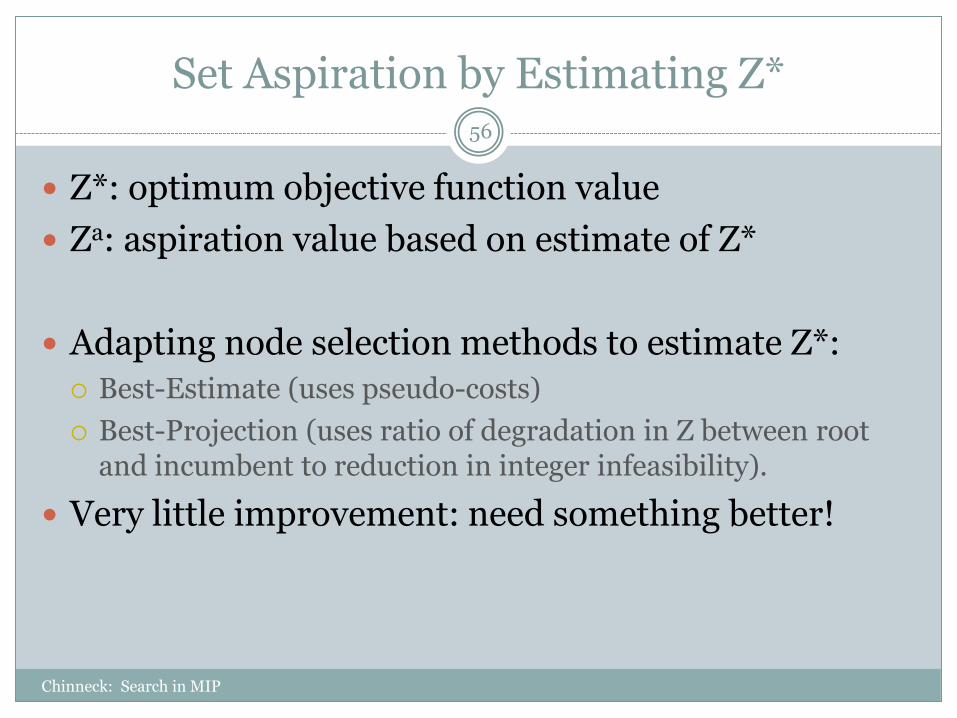
Z*: optimum objective function value
Za: aspiration value based on estimate of Z*
Adapting node selection methods to estimate Z*:
Best-Estimate (uses pseudo-costs)
Best-Projection (uses ratio of degradation in Z between root and incumbent to reduction in integer infeasibility).
Very little improvement: need something better!

New: Projection Based on Depth of Z*
Chinneck: Search in MIP
57
Observation: nodes at depth of Z* have similar value

Frequent Pattern
Chinneck: Search in MIP
58
Zero candidates = feasible solution
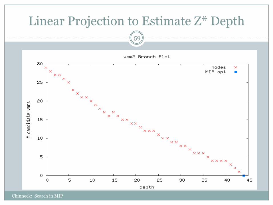
Linear Projection to Estimate Z* Depth
Chinneck: Search in MIP
59

Reconciling Multiple Active Nodes
Chinneck: Search in MIP
60
Each active node has its own projection of Z* depth
Which one should we use?
Frequent pattern of optima: use the shallowest projection!

Method: Linear Extrapolation to Estimate Z*
Chinneck: Search in MIP
61
For every active node with depth ≥ 20 Fit least-squares line to number of candidates vs. depth using
all ancestor nodes
Project depth of closest feasible solution (zero candidates)
k = smallest extrapolated depth over all nodes
Za = max of Zi over all nodes at depth (conservative)
Notes
Za is the aspiration value that is set (minimization)
20 chosen empirically: enough data to extrapolate

Example
Chinneck: Search in MIP
62
Usually close, not perfect...
New: Modified Best Projection Aspiration
Chinneck: Search in MIP
63
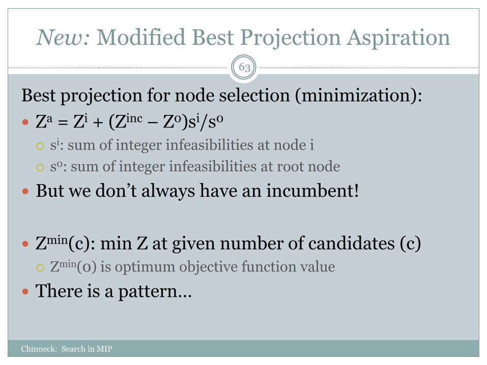
Best projection for node selection (minimization):
Za = Zi + (Zinc – Z0)si/s0
si: sum of integer infeasibilities at node i
s0: sum of integer infeasibilities at root node
But we don’t always have an incumbent!
Zmin(c): min Z at given number of candidates (c)
Zmin(0) is optimum objective function value
There is a pattern…

Projecting Zmin(c)
Chinneck: Search in MIP
64
Modified Best Projection Aspiration
Chinneck: Search in MIP
65
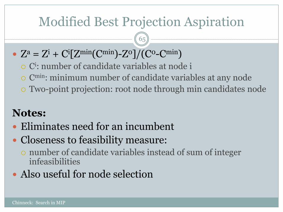
Za = Zi + Ci[Zmin(Cmin)-Z0]/(C0-Cmin) Ci: number of candidate variables at node i
Cmin: minimum number of candidate variables at any node
Two-point projection: root node through min candidates node
Notes:
Eliminates need for an incumbent
Closeness to feasibility measure: number of candidate variables instead of sum of integer
infeasibilities
Also useful for node selection

New: Distribution-based Jumpback
Chinneck: Search in MIP
66
Balance pursuit of both feasibility and optimality
Minimizing: smaller Zi and Ci both desirable
Zi tends to be large where Ci is small, and vice versa
Ranges quite different: how to balance?
Assume independent normal probability distribns
Normalize ranges of Zi and Ci
P(Z ≤ Zi, C ≤ Ci) = FZ(Zi) F
C(Ci)
Choose node n where n = arg miniP(Z ≤ Zi, C ≤ Ci)
i.e. node n has lowest prob. of being “beaten”

Distributions: Gaussian-like
Chinneck: Search in MIP
67

New: Active Node Search Threshold
Chinneck: Search in MIP
68
Advanced node selection can be time-consuming
ANST: switch to simple depth-first backtracking under certain conditions
Rt = (cum. time for node selection)/(cum. time for all else)
If Rt > 0.1, then switch to simple depth-first node selection

Testing Numerous Combinations
Chinneck: Search in MIP
69
Top to Bottom:Node selection | Jumpback | ANST?Mod Best Proj | Mod Best Proj Asp | ANSTDist Node Sel | Mod Best Proj Asp| ANSTDef Best Proj | Def Best Proj AspGLPK defaults

Branching to Force Change
Chinneck: Search in MIP
70
Question: What is the best branching strategy to reach first incumbent quickly?
Force more candidates to integrality at each branch.

Basic Question
Chinneck: Search in MIP
71
You can either:
a) Branch to have largest probability of satisfying constraints in a MIP, or
b) Branch to have smallest probability of satisfying constraints in a MIP.
Which policy leads to the first feasible solution more quickly?

Clue: Active Constraints Variable Selection
Chinneck: Search in MIP
72
Choose candidate variable having greatest impact on the active constraints in current LP relaxation
All other methods look at impact on objective fcn
Reaches integer-feasibility very quickly
Method A:
choose candidate variable appearing in largest number of active constraints, branch up

Clue: “Multiple Choice” Constraints
Chinneck: Search in MIP
73
x1 + x2 + x3 + ... xn {≤,=} 1, where xi are binary
Branch down: other xi can take real values
Branch up: all xi forced to integer values
E.g.: x1 + x2 + x3 + x4 = 1 at (0.25, 0.25, 0.25, 0.25)
Branching on x1 :
Branch down: (0, 0.333, 0.333, 0.333) or others
Branch up: (1, 0, 0, 0) is only solution

New Principle
Chinneck: Search in MIP
74
Branch to Force Change
E.g. branch up on multiple choice constraints
E.g. active constraint branching variable selecn
In general:
Branch to cause change that will propagate to as many candidate variables as possible.
Hope that many will take integer values.

Branching Direction
Chinneck: Search in MIP
75
UP is best. Why?
0
0.1
0.2
0.3
0.4
0.5
0.6
0.7
0.8
0.9
1
1 2 3 4 5 6 7 8 9 10
Fr
ac
tio
n o
f M
od
els
Ratio to Fewest Simplex Iterations
Up vs. Down vs. Closest Integer: All Models
GLPK Default
Up
Down
Closest Integer

New: Probability-Based Branching
Chinneck: Search in MIP
76
Counting integer solutions (Pesant and Quimper 2008)
l ≤ cx ≤ u : l, c, u are integer values, x integer
Example: x1 + 5x2 ≤ 10 where x1, x2 ≥ 0Value of x2 Range for x1 Soln count Soln density
x2=0 [0,10] 11 11/18 = 0.61
x2=1 [0,5] 6 6/18 = 0.33
x2=2 [0] 1 1/18 = 0.06
Total solutions 18
Choose x2 =0 for max prob of satisfying constraint
Is this the best thing to do?

Generalization
Assume:
All variables bounded, real-valued
Uniform distribution within range
Result:
linear combination of variables yields approx. normal distribution for function value
Example: g(x) = 3x1 + 2x2 + 5x3, 0 ≤ x ≤ 5has mean 25, variance 110.83
Plot.... look at g(x) ≤ 12
Chinneck: Search in MIP
77

g(x) = 3x1 + 2x2 + 5x3 ≤ 12, 0 ≤ x ≤ 5
Chinneck: Search in MIP
78
Probability density plot• Cumulative prob of satisfying function in blue

Use for Branching
Chinneck: Search in MIP
79
• Different distributions for DOWN and UP branches due to changed variable ranges
• Different cumulative probabilities of satisfying constraint in each direction
Example:
• Branch on x1=1.5
• Down: x1 range [0,1], p=0.23
• Up: x1 range [2,5], p=0.05
Handling Equality Constraints
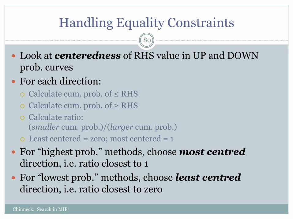
Look at centeredness of RHS value in UP and DOWN prob. curves
For each direction:
Calculate cum. prob. of ≤ RHS
Calculate cum. prob. of ≥ RHS
Calculate ratio: (smaller cum. prob.)/(larger cum. prob.)
Least centered = zero; most centered = 1
For “highest prob.” methods, choose most centreddirection, i.e. ratio closest to 1
For “lowest prob.” methods, choose least centreddirection, i.e. ratio closest to zero
Chinneck: Search in MIP
80

New Branching Direction Methods
Given branching variable, choose direction:
Try UP and DOWN for each active constraint branching variable is in. Choose direction:
LCP: lowest cum. prob. in any active constraint
HCP: highest cum. prob. in any active constraint
LCPV: direction most often having lowest cum. prob.
HCPV: direction most often having highest cum. prob.
Chinneck: Search in MIP
81

Choose Both Variable and Direction
VDS-LCP: choose varb and direction having lowest cum. prob. among all candidate varbs and all active constraints containing them
VDS-HCP: choose varb and direction having highest cum. prob. among all candidate varbs and all active constraints containing them
Chinneck: Search in MIP
82
New: Violation-Based Methods
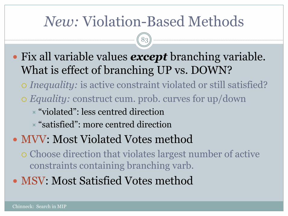
Fix all variable values except branching variable. What is effect of branching UP vs. DOWN?
Inequality: is active constraint violated or still satisfied?
Equality: construct cum. prob. curves for up/down
“violated”: less centred direction
“satisfied”: more centred direction
MVV: Most Violated Votes method
Choose direction that violates largest number of active constraints containing branching varb.
MSV: Most Satisfied Votes method
Chinneck: Search in MIP
83

Experiments
Compare methods in pairs:
Branching to high vs. low prob. of satisfying active constraints
GLPK default included in all comparisons
Branching variable selection: GLPK default
Except for variable-and-direction methods
Chinneck: Search in MIP
84

Chinneck: Search in MIP 85
0
0.1
0.2
0.3
0.4
0.5
0.6
0.7
0.8
0.9
1
1 2 3 4 5 6 7 8 9 10
Fr
ac
tio
n o
f M
od
els
Ratio to Fewest Simplex Iterations
LCP vs. HCP; LCPV vs. HCPV: All Models
GLPK Default
LCP
HCP
LCPV
HCPV
Chinneck: Search in MIP 86
0
0.1
0.2
0.3
0.4
0.5
0.6
0.7
0.8
0.9
1
1 2 3 4 5 6 7 8 9 10
Fr
ac
tio
n o
f M
od
els
Ratio to Fewest Simplex Iterations
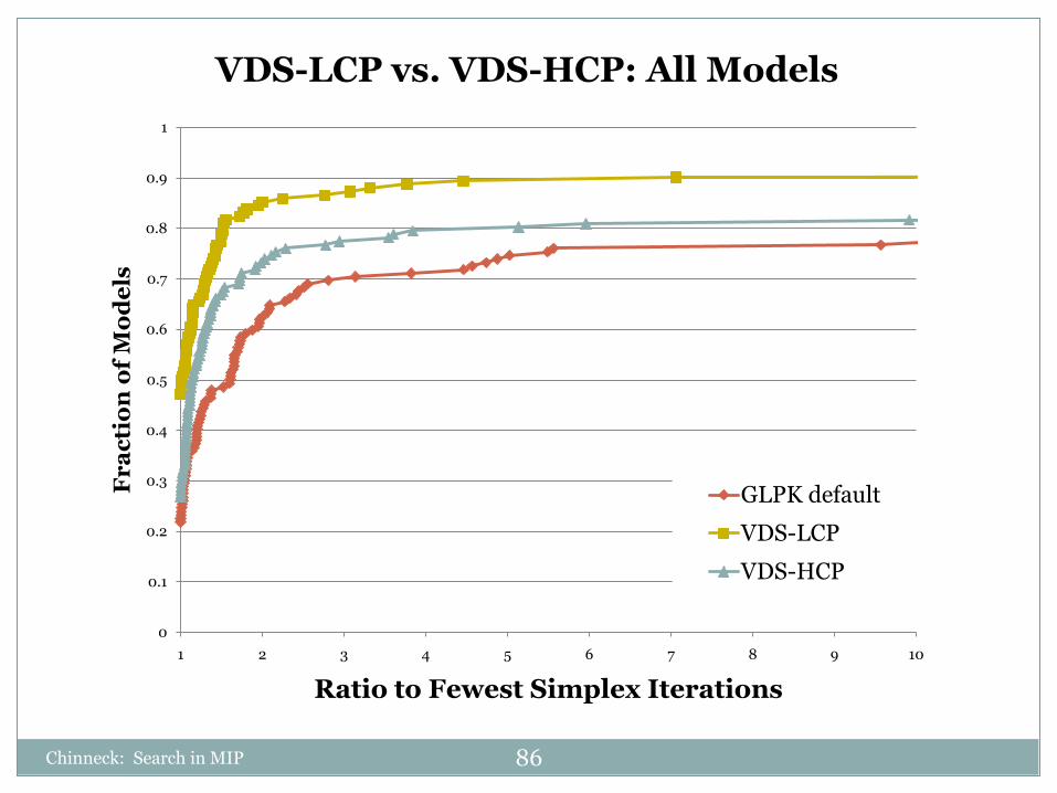
VDS-LCP vs. VDS-HCP: All Models
GLPK default
VDS-LCP
VDS-HCP

VDS Methods With Equality Constraints
Chinneck: Search in MIP
87
0
0.1
0.2
0.3
0.4
0.5
0.6
0.7
0.8
0.9
1
1 2 3 4 5 6 7 8 9 10
Fr
ac
tio
n o
f M
od
els
Ratio Fewest Simplex Iterations
VDS-LCP vs. VDS-HCP: At Least One Equality
GLPK Default
VDS-LCP
VDS-HCP
• VDS-LCP even more dominant
• The centering strategy is effective

Chinneck: Search in MIP 88
0
0.1
0.2
0.3
0.4
0.5
0.6
0.7
0.8
0.9
1
1 2 3 4 5 6 7 8 9 10
Fr
ac
tio
n o
f M
od
els
Ratio to Fewest Simplex Iterations
MVV vs. MSV: All Models
GLPK Default
MSV
MVV
Chinneck: Search in MIP 89
0
0.1
0.2
0.3
0.4
0.5
0.6
0.7
0.8
0.9
1
1 2 3 4 5 6 7 8 9 10
Fr
ac
tio
n o
f M
od
els
Ratio to Fewest Simplex Iterations
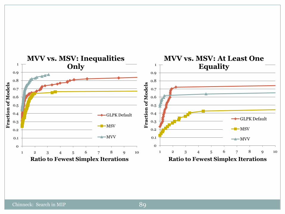
MVV vs. MSV: Inequalities Only
GLPK Default
MSV
MVV
0
0.1
0.2
0.3
0.4
0.5
0.6
0.7
0.8
0.9
1
1 2 3 4 5 6 7 8 9 10
Fr
ac
tio
n o
f M
od
els
Ratio to Fewest Simplex Iterations
MVV vs. MSV: At Least One Equality
GLPK Default
MSV
MVV

Best Methods: A-UP vs. VDS-LCP
Chinneck: Search in MIP
90
0
0.1
0.2
0.3
0.4
0.5
0.6
0.7
0.8
0.9
1
1 2 3 4 5 6 7 8 9 10
Fr
ac
tio
n o
f M
od
els
Ratio to Fewest Simplex Iterations
A-UP vs. VDS-LCP: All Models
GLPK Default
A-UP
VDS-LCP

Branching Up Revisited
UP is good because many models have multiple choice constraints!
104 of 142 (73%) models have at least one
Chinneck: Search in MIP
91
0
0.1
0.2
0.3
0.4
0.5
0.6
0.7
0.8
0.9
1
1 2 3 4 5 6 7 8 9 10
Fr
ac
tio
n o
f M
od
els
Ratio to Fewest Simplex Iterations
At Least One Multiple Choice Constraint
GLPK Default
A-UP
VDS-LCP
A-LCP
A-LCPV
A-MVV
0
0.1
0.2
0.3
0.4
0.5
0.6
0.7
0.8
0.9
1
1 2 3 4 5 6 7 8 9 10
Ratio to Fewest Simplex Iterations
No Multiple Choice Constraints
GLPK Default
A-UP
VDS-LCP
A-LCP
A-LCPV
A-MVV
Conclusions
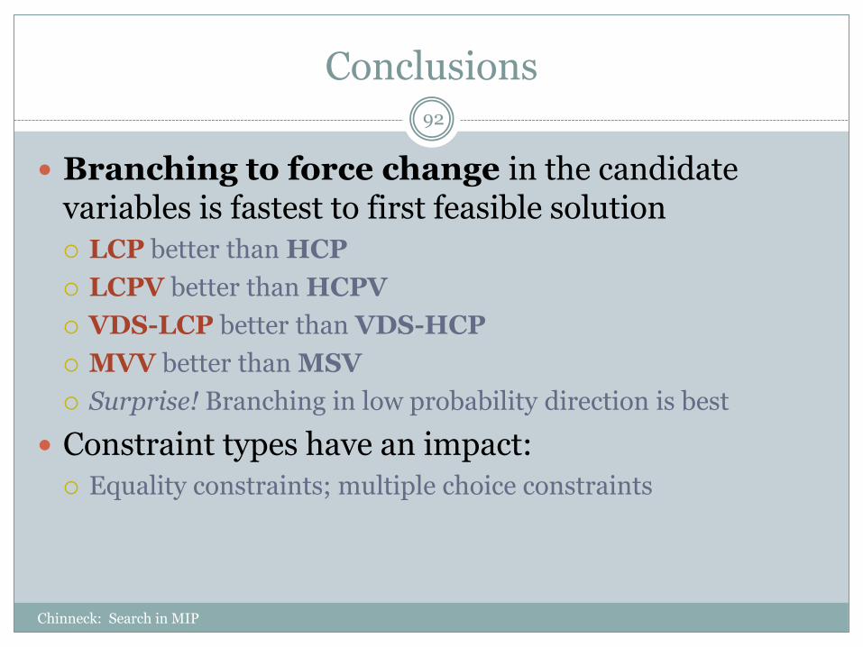
Branching to force change in the candidate variables is fastest to first feasible solution
LCP better than HCP
LCPV better than HCPV
VDS-LCP better than VDS-HCP
MVV better than MSV
Surprise! Branching in low probability direction is best
Constraint types have an impact:
Equality constraints; multiple choice constraints
Chinneck: Search in MIP
92

Observations
Chinneck: Search in MIP
93
MIP:
Linear constraints always satisfied, integrality more difficult
Branch to force integrality as much as possible
Constraint programming:
Integrality always satisfied, constraints more difficult
Branch to satisfy constraints as much as possible

General Disjunctions
Chinneck: Search in MIP
94
Faster integer-feasibility in MIPs by using general disjunctions
Observation: “45 degree” general disjunctions leave no integer solutions in their “interior”

Method
Chinneck: Search in MIP
95
Find 45 degree general disjunction that is: as parallel as possible or
as perpendicular as possible
to active constraint having the most candidate varbs: Active inequality chosen: as parallel as possible
Active equality chosen: as perpendicular as possible
All coefficients must be +1, -1 or 0 for 45 degree Many possibilities
Simple rules try to match/reverse signs in chosen constraint
Branch in the direction that forces change
45 degree general disjunction only when “stuck”

Results
Chinneck: Search in MIP
96
References
Chinneck: Search in MIP
97
J. Pryor and J.W. Chinneck (2011), “Faster Integer-Feasibility in Mixed-Integer Linear Programs by Branching to Force Change", Computers and Operations Research, vol. 38, no. 8, pp. 1143-1152.
D.T. Wojtaszek and J.W. Chinneck (2010), “Faster MIP Solutions via New Node Selection Rules”, Computers and Operations Research, vol. 37, no. 9, pp. 1544-1556.
J. Patel and J.W. Chinneck (2007), "Active-Constraint Variable Ordering for Faster Feasibility of Mixed Integer Linear Programs", Mathematical Programming Series A, vol. 110, pp. 445-474.

A C T I V E C O N S T R A I N T S B R A N C H I N G V A R I A B L E S E L E C T I O N
B R A N C H I N G T O F O R C E C H A N G E
N O G O O D B R A N C H I N G
S T R O N G B R A N C H I N G
Chinneck: Search in MIP
98
Cross-Fertilization

Active Constraints Branching Variable Selection
Chinneck: Search in MIP
99
Constraint Programming
Backdoor variable:
Assigning a value to a backdoor variable simplifies the problem as much as possible
Is the active constraints branching variable selection method choosing a “backdoor” variable?

Branching to Force Change
Constraint Programming:
Fail-first: select varb having fewest remaining legal values
Degree heuristic: select variable appearing in most constraints on other varbs whose values are not yet set
Satisfiability:
MAXO: select literal that appears most often
MOMS: select literal appearing most often in clauses of minimum size
MAMS: combine MAXO and MOMS
Jeroslaw-Wang: weights small clauses more heavily
Chinneck: Search in MIP
100

Nogood Branching
Chinneck: Search in MIP
101
Constraint Programming
Intelligent backtracking
Backtrack on members of the conflict set
Conflict-directed backtracking
The backtrack set is minimal [same as an Irreducible Infeasible Subset of an infeasibility]
Constraint Learning / Nogood Learning
Add constraints based on the minimal infeasible set

Strong Branching
Chinneck: Search in MIP
102
Satisfiability
UP (unit propagation):
Make test assignment for each unassigned literal; count the number of unit propagations triggered
SUP (selective unit propagation):
Reduce testing of literals by first running MAXO, MOMS, MAMS, Jeroslaw-Wang to identify at most 4 candidates