sean mcnamara hans j. herrmann geometrical derivation · pdf filehans j. herrmann geometrical...
TRANSCRIPT

Acta Mech 205, 171–183 (2009)DOI 10.1007/s00707-009-0172-5
Andrés A. Peña · Pedro G. Lind · Sean McNamara ·Hans J. Herrmann
Geometrical derivation of frictional forces for granularmedia under slow shearing
Received: 23 September 2007 / Revised: 5 May 2008 / Published online: 4 April 2009© Springer-Verlag 2009
Abstract We present an alternative way to determine the frictional forces at the contact between two particles.This alternative approach has its motivation in a detailed analysis of the bounds on the time integration step inthe discrete element method for simulating collisions and shearing of granular assemblies. We show that, instandard numerical schemes, the upper limit for the time integration step, usually taken from the average timetc of one contact, is in fact not sufficiently small to guarantee numerical convergence of the system duringrelaxation. In particular, we study in detail how the kinetic energy decays during the relaxation stage andcompute the correct upper limits for the time integration step, which are significantly smaller than the onescommonly used. In addition, we introduce an alternative approach based on simple relations to compute thefrictional forces that converges even for time integration steps above the upper limit.
1 Introduction
One of the standard approaches to model the dynamics of granular media is to use the discrete element method(DEM) [1–3], e.g., to study shear [4–8]. Some problems may arise due to the need to use large time integrationsteps to perform numerical simulations with reasonable computational effort without compromising the overallconvergence of the numerical scheme chosen.
An efficient method for the numerical integration of systems of coupled differential equations, particularlysuited for granular media [1] is the so-called Gear algorithm. One important feature of the Gear algorithm isits numerical stability, making it particularly suited for granular particle systems where short range interac-tions co-exist with strong gradients. This algorithm consists of two main steps, one where particle positionsand higher-order derivatives are predicted and another where they are corrected. A short description of this
A. A. Peña · P. G. Lind · S. McNamaraInstitute for Computational Physics, Universität Stuttgart, Pfaffenwaldring 27, 70569 Stuttgart, Germany
A. A. PeñaBilfinger Berger GmbH, Civil, Structural Design, 65189 Wiesbaden, Germany
P. G. LindCentro de Física Teórica e Computacional, Av. Prof. Gama Pinto 2, 1649-003 Lisbon, Portugal
H. J. HerrmannDepartamento de Física, Universidade Federal do Ceará, Fortaleza, Ceará 60451-970, Brazil
H. J. Herrmann (B)Computational Physics, IfB, HIF E12, ETH Hönggerberg, 8093 Zurich, SwitzerlandE-mail: [email protected]

172 A. A. Peña et al.
algorithm is given in the Appendix. Usually, one assumes an upper limit for the admissible integration stepsbased on empirical reasoning [9].
While such numerical schemes chosen to integrate the equations of motion are of importance, it is known[1] that a substantial part of the computation efforts is spent on the evaluation of the forces acting on eachparticle at each time step. For that reason, as we will see, the time integration step used for the computation ofthe forces is sometimes larger than the one of the integration scheme for the equations of motion. While sucha difference is not critical in some shear systems, for slow shearing it plays a non-negligible role.
For slow shearing, the convergence of numerical schemes is particularly important when studying forinstance the occurrence of avalanches [8] and the emergence of ratcheting in cyclic loading [10].
In this paper we show that the time integration step able to guarantee convergence of the numericalscheme, must in general be smaller than a specific upper limit, significantly below the commonly acceptedvalue [5,9,11]. This upper limit strongly depends on (i) the accuracy of the approach used to calculate frictionalforces between particles, (ii) on the corresponding duration of the contact and (iii) on the number of degrees offreedom. To illustrate this fact, we address the specific case of slow shearing, for which the above limit is toosmall to allow for reasonable computation time. Here, we concentrate on the accuracy of the total kinetic energyof the system in a stress-controlled test. The total kinetic energy is one of the important quantities in severalsystems under slow shearing, such as tectonic systems, for which the study and forecasting of avalanches andearthquakes rely significantly on the accurate computation of the kinetic energy released by the system.
Additionally, we show that the need of a small time integration step is related to the scheme used to computethe frictional forces, namely the Cundall spring model. To overcome the shortcoming present in the Cundallspring model, we propose an alternative approach that corrects the frictional contact forces, when large timeintegration steps are taken. In this way, we enable the use of considerably larger integration steps, assuring atthe same time the convergence of the integration scheme used for the equations of motion.
We start in Sect. 2 by presenting in some detail the DEM [1,9,12]. Sections 3 and 4 describe, respectively,the dependence on the time integration step and the improved algorithm. Discussions and conclusions aregiven in Sect. 5.
2 The model
We consider a two-dimensional system of polygonal particles, each one having two linear and one rotationaldegree of freedom. The evolution of the system is given by Newton’s equations of motion, where the resultingforces and moments acting on each particle i are given by the sum of all forces and moments applied on thatparticle:
mi r i =∑
c
Fci +
∑
cb
Fbi , (1a)
Ii θ i =∑
c
lci × Fc
i +∑
cb
lbi × Fb
i , (1b)
where mi denotes the mass of particle i , Ii its moment of inertia, and l the branch vector which connects thecenter of mass of the particle to the application point of the contact force Fc
i or boundary force Fbi . The sum
in c is over all the particles in contact with polygon i , and the sum in cb is over all the vertices of polygon i incontact with the boundary. One integrates Eq. (1) for all particles i = 1, . . . , N and obtains the evolution oftheir centers of mass r i and rotation angles θi .
Further, during loading, particles tend to deform each other. This deformation of the particles is usuallyreproduced by letting them overlap [1,12], as illustrated in Fig. 1. The overlap between each pair of particles isconsidered to fully characterize the contact. Namely, the normal contact force is assumed to be proportional tothe overlap area [13] and its direction perpendicular to the plane of contact, which is defined by the intersectionbetween the boundaries of the two particles.
All the dynamics is deduced from the contact forces acting on the particles. The contact forces, Fc, eitherbetween particles or with the boundary, are decomposed into their elastic and viscous contributions, Fe andFv , respectively, yielding Fc = Fe + Fv .
The viscous force is important for maintaining the numerical stability of the method and to take into accountdissipation at the contact. This force is calculated as [12]
Fv = −mrνvc, (2)
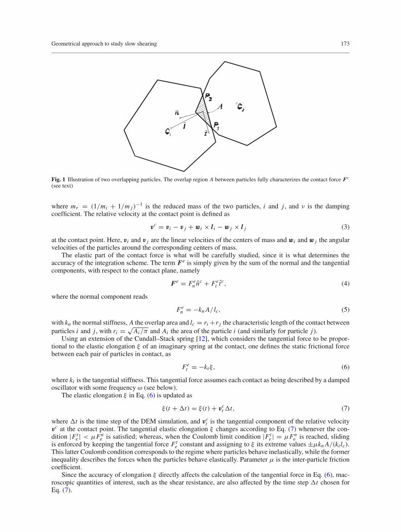
Geometrical approach to study slow shearing 173
Fig. 1 Illustration of two overlapping particles. The overlap region A between particles fully characterizes the contact force Fc
(see text)
where mr = (1/mi + 1/m j )−1 is the reduced mass of the two particles, i and j , and ν is the damping
coefficient. The relative velocity at the contact point is defined as
vc = vi − v j + wi × l i − w j × l j (3)
at the contact point. Here, vi and v j are the linear velocities of the centers of mass and wi and w j the angularvelocities of the particles around the corresponding centers of mass.
The elastic part of the contact force is what will be carefully studied, since it is what determines theaccuracy of the integration scheme. The term Fe is simply given by the sum of the normal and the tangentialcomponents, with respect to the contact plane, namely
Fe = Fen nc + Fe
t t c, (4)
where the normal component reads
Fen = −kn A/ lc, (5)
with kn the normal stiffness, A the overlap area and lc = ri +r j the characteristic length of the contact betweenparticles i and j , with ri = √
Ai/π and Ai the area of the particle i (and similarly for particle j).Using an extension of the Cundall–Stack spring [12], which considers the tangential force to be propor-
tional to the elastic elongation ξ of an imaginary spring at the contact, one defines the static frictional forcebetween each pair of particles in contact, as
Fet = −ktξ, (6)
where kt is the tangential stiffness. This tangential force assumes each contact as being described by a dampedoscillator with some frequency ω (see below).
The elastic elongation ξ in Eq. (6) is updated as
ξ(t + �t) = ξ(t) + vct �t, (7)
where �t is the time step of the DEM simulation, and vct is the tangential component of the relative velocity
vc at the contact point. The tangential elastic elongation ξ changes according to Eq. (7) whenever the con-dition |Ft
e | < µFne is satisfied; whereas, when the Coulomb limit condition |Ft
e | = µFne is reached, sliding
is enforced by keeping the tangential force Fte constant and assigning to ξ its extreme values ±µkn A/(kt lc).
This latter Coulomb condition corresponds to the regime where particles behave inelastically, while the formerinequality describes the forces when the particles behave elastically. Parameter µ is the inter-particle frictioncoefficient.
Since the accuracy of elongation ξ directly affects the calculation of the tangential force in Eq. (6), mac-roscopic quantities of interest, such as the shear resistance, are also affected by the time step �t chosen forEq. (7).

174 A. A. Peña et al.
As said above, in DEM, one of the numerical integration schemes usually used to solve the equations ofmotion above is the Gear’s predictor–corrector scheme [9]. This scheme consist of three main stages, namelyprediction, evaluation, and correction (see the Appendix for details). Using this numerical scheme we integrateequations of the form r = f (r, r), using a fifth order predictor–corrector algorithm that has a numerical errorproportional to (�t)6 for each time integration step [9]. However, as will be seen in Sect. 3, (�t)6 is not thenumerical error of the full integration scheme, since Eq. (6), used to calculate the frictional force, is of order(�t)2.
For a certain value of normal contact stiffness kn , almost any value for the normal damping coefficientνn might be selected. Their relation defines the restitution coefficient ε obtained experimentally for variousmaterials [14]. The restitution coefficient is given by the ratio between the relative velocities after and beforea collision. In particular, the normal restitution coefficient εn can be written as a function of kn and νn [15],namely
εn = exp (−πη/ω) = exp
(− π√
4mr kn/ν2n − 1
), (8)
where ω =√
ω20 − η2 is the frequency of the damped oscillator, with ω0 = √
kn/mr the frequency of theelastic oscillator, mr the reduced mass and η = νn/(2mr ) the effective viscosity. The tangential component εtof the restitution coefficient is defined similarly using kt and νt in Eq. (8).
Therefore, a suitable closed set of parameters for this model are the ratios kt/kn and εt/εn , νt/νn , togetherwith the normal stiffness kn and the interparticle friction µ. For simplicity we will always take νt/νn = kt/knwhich is assumed to be constant, as done in previous studies [6].
The entire algorithm above relies on a proper choice of the integration step �t , which should neither betoo large to avoid divergence of the integration nor too small avoiding unreasonably long computational time.The determination of the optimal time integration step varies from case to case and one usually assumes thepossible main criteria to estimate an upper bound for admissible time integration steps.
The first criterion is to use the characteristic period of oscillation [9], defined as
ts = 2π
√〈m〉kn
, (9)
where 〈m〉 is the smallest particle mass in the system. For a fifth order predictor–corrector integration scheme,it is usually accepted that a safe time integration step should be below a threshold of �t < ts/10 [9].
The second criterion is to extract the threshold from local contact events [5,11,15], namely from thecharacteristic duration of a contact:
tc = π√ω2
0 − η2. (10)
Both criteria can be assumed to be equivalent, since typically tc � ts/2, and therefore in such cases, oneconsiders as an admissible time integration steps such that �t < tc/5 [15,16].
In the next section we will study in detail the integration for different values of the model parameters.
3 The choice of the time integration step
We simulate the relative motion of two plates shearing against each other [7,8,13]. Considering a system of 256particles as illustrated in Fig. 2, where both top and bottom boundaries move in opposite directions with a con-stant shear rate γ . The top and bottom layer of the sample have fixed boundary conditions, while horizontallywe consider periodic boundary conditions. The volumetric strain is suppressed, i.e., the vertical position of thewalls is fixed and there is no dilation. The particles of the fixed boundary are not allowed to rotate or moveagainst each other. The shear rate is γ = 1.25×10⁻⁵s−1, the parameter values are kn = 400 N/m, εn = 0.9875,and µ = 0.5. The relation kt/kn is chosen such that kt < kn , similar to previous studies [12,15,17], namelykt/kn = νt/νn = 1/3, which when substituted in Eq. (8) yields εt/εn = 1.0053.

Geometrical approach to study slow shearing 175
Vx / 2
Vx / 2
hconst
Fig. 2 Sketch of the system of 256 particles (light particles, green in color) under shearing of top and bottom boundaries (darkparticles, blue in color). Horizontally periodic boundary conditions are considered and a constant low shear rate is chosen (seetext)
By integrating such a system of particles using the scheme described in the previous section, one can easilycompute the kinetic energy Ek of a given particle i ,
Ek(i) = 1
2
(mi r2
i + Iiω2i
), (11)
where the velocity r is computed from the predictor–corrector algorithm, Ii is the moment of inertia of thepolygon and ωi is the angular velocity. The total kinetic energy of the full system of particles is given just bythe sum of Ek(i) over all the particles.
In Fig. 3, we show the evolution of the total kinetic energy for two different �t/tc = 13/2,500tc and13/500tc. This kinetic energy is of the same order of magnitude as the corresponding elastic energy. As onesees, frictionless particles (Fig. 3a, c) have an Ek that does not change for different integration steps, whilewhen µ = 0.5 (Fig. 3b, d) the evolution of Ek strongly depends on �t . In Fig. 3e we plot the cumulativedifference �Ek between the values of Ek taken for each time integration step. Here, one sees that in the absenceof friction �Ek is significantly lower then when friction is present.
From Fig. 3, one concludes that the expected upper limit ∼ tc/5, usually assumed and mentioned inthe previous section, is still too large to guarantee convergence of the integration scheme when friction isconsidered.
To obtain a proper time integration step as function of the parameters of our model we next perform acareful analysis. If the commonly upper bound considered for the integration steps are valid in large systems,they must also be valid for single pairs of overlapping particles, even in the case when particles have a regularform, say discs. We will show that even in such small and simple systems lower bounds for the time integrationstep must be considered. In particular, at the usual bounds the kinetic energy of a stress-controlled test of twoparticles still does not decay at the proper rate.
As sketched in Fig. 4, we consider the simple situation of two circular particles and study the kinetic energyof one of them under external forcing, as sketched in Fig. 4. We start with two touching discs, i and j , whereone of them, say i , remains fixed, while the other is subject to a force F perpendicular to its surface (no externaltorque is induced) along the x-axis. As a result of this external force, the disc j undergoes rotation. The contactforce is obtained from the corresponding springs that are computed, as described in Sect. 2, and acts againstthe external force. This results in an oscillation of disc j till relaxation (dashed circle in Fig. 4) with a finalcenter of mass displacement of �R and a rotation around the center of mass of �θ . Since F is kept constant,the procedure is stress controlled.

176 A. A. Peña et al.
1e-08
1e-06
0.0001
0.01
Ek
1000 1100
t
1e-08
1e-06
0.0001
0.01
Ek
0 200 400 600 800 1000 1200
t1e-21
1e-181e-15
1e-12
1e-091e-06
∆Ek µ=0
µ=0.5
1000 1100 1200
t
(a) (b)
(c) (d)
(e)
Fig. 3 Dependence of the Gear’s numerical scheme on the time integration step �t and the friction coefficient µ, by plotting thekinetic energy Ek as a function of time, for a �t/tc = 13/2,500tc and µ = 0 (no friction), b �t/tc = 13/2,500tc and µ = 0.5,c �t/tc = 13/500tc and µ = 0, and d �t/tc = 13/500tc and µ = 0.5. In e we show the difference between the values of Ekobtained with the two values of �t . Here, kn = 400 and the parametric relations in Eq. (9) and (10) are used (see text)
r∆θ F
Y
X
a
a
r
rj
i
∆
Rij
i
j
F
−FV
V
Fig. 4 Sketch of the stress-controlled test of two particles (discs). The particle located at r i remains fixed, while the particle atr j is initially touching particle i . The vector Ri j connecting the center of mass of particles i and j is initially oriented 45o withrespect to the x-axis. After applying the constant force F to disc j , the system relaxes to a new position (dashed circumference).Between its initial and final position particle j undergoes a displacement �r and a rotation �θ (see text). Forces FV and −FVact on the upper and lower particle to balance the reaction from the wall. So the relaxation depends only on the force F
For the two discs sketched in Fig. 4, we plot in Fig. 5 the kinetic energy as a function of time, from thebeginning until relaxation, using different integration steps, namely �t/tc = 10−1, 2×10⁻², 10−2, 10−3, and10−4. As we see, the kinetic energy decays exponentially,
Ek(t) = E (0)k exp
(− t
tR(�t)
), (12)
where tR is a relaxation time whose value clearly depends on the time integration step �t . As illustrated in theinset of Fig. 5, this change in tR is not observed when friction is absent (µ = 0), since no tangential forces areconsidered (Ft
e = 0).Next, we will show that this dependence of tR on �t vanishes for
�t � Tt (µ)tc, (13)

Geometrical approach to study slow shearing 177
10000 20000 30000t
1e-15
1e-12
1e-09
1e-06
0.001
1
1000
Ek
∆t=1e-1∆t=2e-2∆t=1e-2∆t=1e-3∆t=1e-4
0 5000 10000 15000t
1e-151e-121e-091e-060.001
11000
Ek
Fig. 5 The relaxation of the system of two discs sketched in Fig. 4. Here, we plot the kinetic energy Ek as a function of time t(in units of tc) for different integration increments �t and using a stiffness kn = 4 × 10⁸ N/m and a friction coefficient µ = 500.The large µ value is chosen so that the system remains in the elastic regime. As one sees, the relaxation time tR converges to aconstant value when �t is sufficiently small (see text). This discrepancy between the values of tR when different time integrationsteps are used does not occur in the absence of friction (µ = 0), as illustrated in the inset. The slope of the straight lines is −1/tR(see Eq. 12)
0.0001 0.001 0.01 0.1
∆t/tc
1400
1450
1500
1550
1600
1650
1700
1750
t R /t
c kn=1
kn=50
kn=200
kn=4e4
kn=4e8
Tt
Fig. 6 The relaxation time tR (in units of tc) as a function of the normalized time integration step �t/tc, where the contact timetc is defined in Eq. (10). Here, the friction coefficient is kept fixed µ = 500 and different stiffnesses kn (in units of N/m) areconsidered. The quotient �t/tc collapses all the curves for different kn . As a final result one finds a constant Tt = 10−3 (dashedvertical line)
where Tt (µ) is a specific function that can only depend on µ, since from dimensional analysis it is clear thatit is independent of kn .
Figure 6 shows the relaxation time tR of the kinetic energy of the two-particle system for different valuesof stiffnesses, namely for kn = 1, 50, 200 × 104 and 108 N/m. For all kn values, one sees that, for decreasing�t , the relaxation time tR increases until it converges to a maximum. The stabilization of tR occurs when �t

178 A. A. Peña et al.
1e-05 0.0001 0.001 0.01 0.1
∆ t/tc
0
200
400
600
800
t R /t
c
kn=1
kn=50
kn=200
kn=4e4
kn=4e8
0.0001 0.001 0.01 0.1
∆ t/tc
µ=0.005µ=0.05µ=0.5µ=5µ=50µ=500
µ=0(a)
(b)Tt T
t
Fig. 7 The relaxation time tR (in units of tc) of the kinetic energy as a function of the normalized time integration step �t/tc,when rotation is suppressed. a µ = 500 and different values of kn and for b kn = 4 × 10⁸ and different values of µ. The dashedhorizontal line µ = 0 in b indicates the relaxation time of the kinetic energy in the absence of friction (see text)
is small compared to the natural period 1/ω0 of the system. We define Tt as the largest value of �t for whichwe have this maximal relaxation time.
Further, all curves can be collapsed by using the normalized time integration step �t/tc. From Eq. (10)we calculate the contact times corresponding to these kn values as tc = 1.969, 0.278, 0.139, 9.8 × 10⁻², and9.8 × 10−5 s, respectively. Notice from Eq. (10) that the relaxation time scales with the stiffness as tc ∼ k−1/2
n(see Eq. 10).
From Fig. 6 one can conclude that the relaxation time converges when the time integration step obeysEq. (13) with Tt = 10−3 (dashed vertical line). In Fig. 6 both translation and rotation of particles are con-sidered. The rotation of particles is usually of crucial interest, for instance to simulate rolling [7,18]. Butsuppressing rotation can also be of interest, for instance when simulating fault gouges: by hindering the rota-tion of particles, one can mimic young faults where a strong interlocking between the constituent rocks isexpected [7].
To study this scenario, we present in Fig. 7a the relaxation time for the same parameter values as in Fig. 6,now disabling rotation. Here, we obtain a constant Tt = 10−4 also, independent of kn , one order of magnitudesmaller than the previous value in Fig. 6. In other words, when rotation is suppressed, one must consider timeintegration steps typically one order of magnitude smaller than in the case when the discs are able to rotate.This can be explained as follows.
Though simulations do not require very small integration time steps when angular quantities are not takeninto account, when suppressing rotation, one restricts the system to have a single degree of freedom. This restric-tion is done by enforcing at each time step a zero angular displacement in the predictor–corrector scheme forthe particle under stress controlled test. Such a scenario is equivalent to the introduction of an additional forcein the moving particle, preventing it to rotate. Thus, while this force induces faster relaxation, it varies duringthe simulation making the system more sensitive to the time integration step, i.e., yielding a smaller bound Tt .By comparing Fig. 7a with Fig. 6, one sees that the relaxation time tR is smaller when rotation is suppressed.
From the bounds on the integration steps obtained above, one realizes that, in general, the correct timeintegration step must be significantly smaller than usually assumed.
While Fig. 7a clearly shows that tR does not depend on the stiffness kn , from Fig. 7b one sees that the sameis not true for the friction coefficient µ. Indeed, from Fig. 8a one sees that there is a change of the relaxationtime around µ = 1. Here, the values correspond to a normalized time integration step �t/tc = 10−5 for whichtR has already converged. This transition, which is not observed when rotation is considered (not shown),occurs since for larger values of µ > 1, one has Ft > Fn , and therefore the frictional force increases anddrives the system to relax faster. Further, with rotation one observes a larger tR because there is an additionaldegree of freedom that also relaxes.
We also check the dependence of the relaxation time on the stiffness ratio kt/kn and on the restitutioncoefficient ratio εt/εn . For the stiffness ratio, we find that the convergence to a stationary value of tR is faster

Geometrical approach to study slow shearing 179
0.01 1 100µ
720
740
760
780
800
t R /tc
0.1 1
kt /kn
0
1000
2000
3000
1 1.1 1.2 1.3 1.4 1.5
εt /en
20
40
60
80
100
(a) (b) (c)
Fig. 8 The relaxation time tR (in units of tc) as a function a of the friction coefficient µ when rotation is suppressed, withkn = 4 × 10⁸ N/m which corresponds to a contact time tc = 9.8 × 10⁻⁵ s, b of the stiffness ratio kt/kn with µ = 500 andεt/εn = 1.0053 and c of the restitution coefficients ratio εt/εn with µ = 500 and kt/kn = 1/3. The normalized time integrationstep is �t/tc = 10−5. Dotted line in a indicates the approximate maximum relevant value of µ in shearing systems
for large stiffness ratio as kt/kn → 1, yielding larger values of Tt . Further, the stationary value of tR log-arithmically decreases with the stiffness ratios (see Fig. 8b), which can be explained from direct inspectionof Eq. (8). Figure 8c, showing the relaxation time as a function of the ratio εt/εn for fixed µ = 500 andkt/kn = 1/3, can be explained similarly as in Fig. 8b. Here, the dependence of the stationary value of tR onεt/εn is approximately exponential.
All the correct relaxation times found above are obtained for the upper bound Tt = 10−3. Further, wealso notice that the results above were taken whenever the condition |Ft
e | < µFne is satisfied, since only in
that case Eq. (7) is used (see Sect. 2). This fact indicates that the improvements in the algorithm should beimplemented when computing the elastic component of the tangential contact force, in Eq. (7), as explainedin the next section.
4 Improved approach to integrate the contact force
In this section we will describe a technique to overcome the need of very small time integration steps. Asshown previously, when using Cundall’s spring [4], the relaxation time of the two particles only convergeswhen �t is a small fraction Tt of the contact time tc. This is due to the fact that the elastic elongation is assumedto be linear in �t , i.e., the finite difference scheme in Eq. (7) is of very low order, (�t)2, compromising theconvergence of the Gear’s numerical scheme that is of order (�t)6. Therefore, the most plausible way toimprove our algorithm is by choosing a different expression to compute the elastic tangential elongation ξwithout using Eq. (7). Recently, it was reported [10] that the elastic potential energy stored in the contact ispath-dependent. Consequently, an accurate computation of the frictional force would not be improved by anintegration scheme—that is also path dependent—but, instead, we must assure that the computation of thefrictional force does not depend on the time integration step.
We will introduce an expression for ξ that contains only the quantities computed in the predictor step. Inthis way we guarantee that ξ has errors of the order of (�t)6, instead of (�t)2, as it is the case of Eq. (7). Letus illustrate our approach on the simple system of two discs considered in the previous section (see Fig. 4).
On one side, if rotation is not allowed, the elastic elongation ξ depends only on the relative position of thetwo particles. In this case we substitute Eq. (7) by the expression
ξ(tr)j (t + �t) = ξ
(tr)j (t) + ai
ai + a j(R p
i j (t + �t) − R pi j (t)) × t c, (14)

180 A. A. Peña et al.
1e-05 0.0001 0.001 0.01 0.1
∆t/tc
800
1200
1600
2000
tR
Only RotationOnly TranslationRotation+Translation
Fig. 9 The relaxation time tR (in units of tc) using Eqs. (14) and (15) between two discs, as illustrated in Fig. 4. For the three caseswhen considering only rotation, only translation or both, the relaxation time remains constant independent of the time integrationstep
where ai and a j are the radii of the discs i and j , respectively, Ri j is the vector joining both centers of massand points in the direction i → j (see Fig. 4). The index p indicates quantities derived from the coordinatescomputed at the predictor step.
On the other side, if Ri j is kept constant and only rotation is possible, the particle j will have an elongationξ that depends only on its rotation between time t and the predictor step:
ξ(rot)j (t + �t) = ξ
(rot)j (t) + (θ
pj (t + �t) − θ
pj (t))a j , (15)
where θ p and θ(t) are the rotation angles of particle j till the predictor step and time step t , respectively.When both translation and rotation of particle j occur, then the elongation is the superposition of both
contributions, yielding ξ j = ξ(tr)j + ξ
(rot)j . Thus, using the expressions in Eqs. (14) and (15) one avoids the
truncation error, typically of the order of (�t)2, inherent to the Cundall spring model (see Eqs. 6 and 7).Figure 9 shows the relaxation time tR as a function of the time integration step for the three situations
above, namely when only rotation is considered, when only translation is considered and when both rotationand translation are allowed. As we see for all these cases, the relaxation time is independent on the time inte-gration step. This is due to the fact that all quantities in the expression for ξ above are computed at the predictorstep which has an error of the order of (�t)6, i.e., the error (�t)2 introduced in Eq. (7) is now eliminated.Therefore, with the expressions in Eqs. (14) and (15) one can use time integration steps significantly largerthan with the original Cundall spring.
When considering discs, one does not take into account the shape of the particles. Next, we consider themore realistic situation of irregular polygonal-shaped particles. Motion of rigid particles with polygonal shapeis more complicated than that of simple discs, since the contact point no longer lies on the vector connectingthe centers of mass. Further, for polygons, one must also be careful when decomposing the dynamics of eachparticle into translation and rotation around its center of mass. This implies recalculating each time the positionof the center of mass (only from translation) and the relative position of the vertices (only from rotation).
Therefore, for the translational contribution ξ (tr) in Eq. (14), we compute the overlap area between thetwo particles at t and at the predictor step. The overlap area is in general a polygon with a geometrical centerthat can be computed also at time t and the subsequent predictor step, yielding rc(t) and r p
c , respectively. Theincrement for the translational contribution will be just the tangential projection (rc(t) − r p
c ) × t c. Similarly,the contribution from the (polygonal) particle rotation is computed by determining branch vectors, rb(t) andr p
b , defined as the vectors joining the center of the particle and the center of the overlap area at time step tand the predictor step, respectively. Computing the branch vector at t and at the predictor step, one derivesthe angle defined by them, namely θ = arccos
(r p
b × rb(t)/(rpb rb(t))
), where r p
b and rb(t) is the norm of thecorresponding branch vectors and the average value (r p
b − rb(t))/2, yielding an increment in Eq. (15) givenby θ(r p
b − rb(t))/2.Figure 10 compares how the relaxation time varies with the normalized time step when the original Cundall
approach is used (squares) and when our improved approach is introduced (circles). Clearly, the dependence
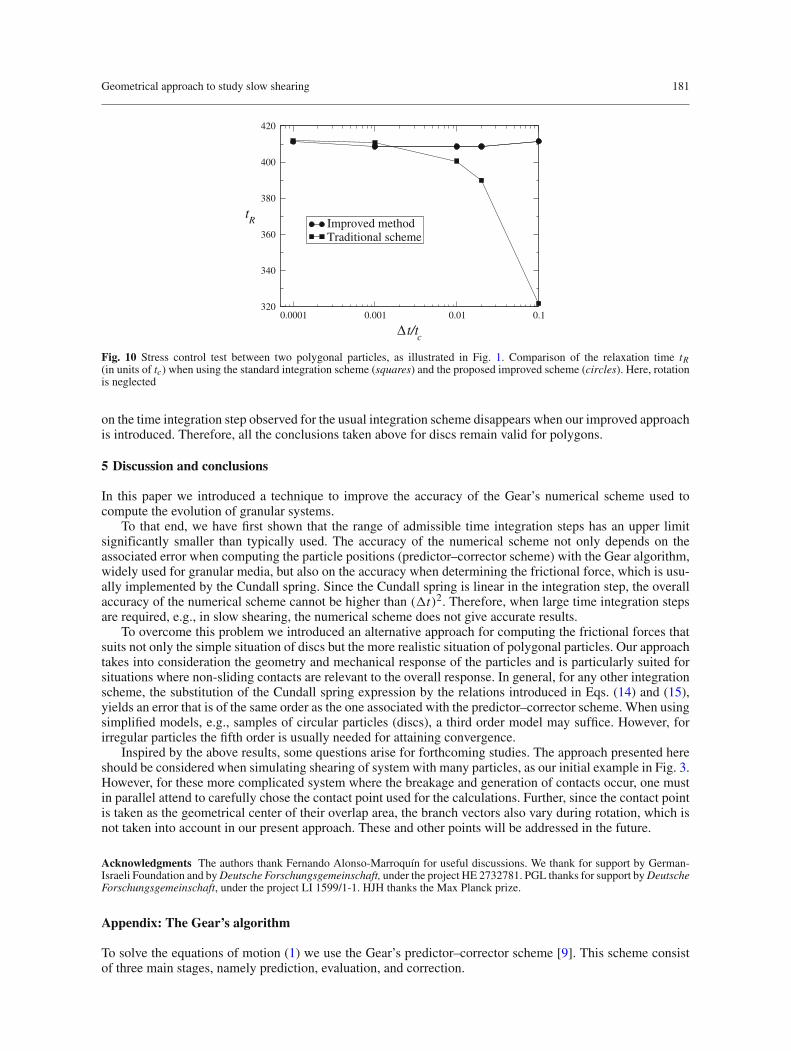
Geometrical approach to study slow shearing 181
0.0001 0.001 0.01 0.1
∆ t/tc
320
340
360
380
400
420
tR Improved method
Traditional scheme
Fig. 10 Stress control test between two polygonal particles, as illustrated in Fig. 1. Comparison of the relaxation time tR(in units of tc) when using the standard integration scheme (squares) and the proposed improved scheme (circles). Here, rotationis neglected
on the time integration step observed for the usual integration scheme disappears when our improved approachis introduced. Therefore, all the conclusions taken above for discs remain valid for polygons.
5 Discussion and conclusions
In this paper we introduced a technique to improve the accuracy of the Gear’s numerical scheme used tocompute the evolution of granular systems.
To that end, we have first shown that the range of admissible time integration steps has an upper limitsignificantly smaller than typically used. The accuracy of the numerical scheme not only depends on theassociated error when computing the particle positions (predictor–corrector scheme) with the Gear algorithm,widely used for granular media, but also on the accuracy when determining the frictional force, which is usu-ally implemented by the Cundall spring. Since the Cundall spring is linear in the integration step, the overallaccuracy of the numerical scheme cannot be higher than (�t)2. Therefore, when large time integration stepsare required, e.g., in slow shearing, the numerical scheme does not give accurate results.
To overcome this problem we introduced an alternative approach for computing the frictional forces thatsuits not only the simple situation of discs but the more realistic situation of polygonal particles. Our approachtakes into consideration the geometry and mechanical response of the particles and is particularly suited forsituations where non-sliding contacts are relevant to the overall response. In general, for any other integrationscheme, the substitution of the Cundall spring expression by the relations introduced in Eqs. (14) and (15),yields an error that is of the same order as the one associated with the predictor–corrector scheme. When usingsimplified models, e.g., samples of circular particles (discs), a third order model may suffice. However, forirregular particles the fifth order is usually needed for attaining convergence.
Inspired by the above results, some questions arise for forthcoming studies. The approach presented hereshould be considered when simulating shearing of system with many particles, as our initial example in Fig. 3.However, for these more complicated system where the breakage and generation of contacts occur, one mustin parallel attend to carefully chose the contact point used for the calculations. Further, since the contact pointis taken as the geometrical center of their overlap area, the branch vectors also vary during rotation, which isnot taken into account in our present approach. These and other points will be addressed in the future.
Acknowledgments The authors thank Fernando Alonso-Marroquín for useful discussions. We thank for support by German-Israeli Foundation and by Deutsche Forschungsgemeinschaft, under the project HE 2732781. PGL thanks for support by DeutscheForschungsgemeinschaft, under the project LI 1599/1-1. HJH thanks the Max Planck prize.
Appendix: The Gear’s algorithm
To solve the equations of motion (1) we use the Gear’s predictor–corrector scheme [9]. This scheme consistof three main stages, namely prediction, evaluation, and correction.

182 A. A. Peña et al.
In the prediction stage the position, velocities, and higher-order time derivatives are updated by expansions ofthe corresponding Taylor series using the current values of these quantities [9,19]. For the position r of thecenter of mass these equations read
r(t+�t),p = r(t) + r(t) �t + r(t)�t2
2! + r i i i(t)
�t3
3! + r iv(t)
�t4
4! + rv(t)
�t5
5! ,
r(t+�t),p = r(t) + r(t) �t + r i i i(t)
�t2
2! + r iv(t)
�t3
3! + rv(t)
�t4
4! ,
r(t+�t),p = r(t) + r i i i(t) �t + r iv
(t)�t2
2! + rv(t)
�t3
3! ,
r i i i(t+�t),p = r i i i
(t) + r iv(t) �t + rv
(t)�t2
2! ,
r iv(t+�t),p = r iv
(t) + rv(t) �t,
rv(t+�t),p = rv
(t).
From the equations above, one extracts a predicted position r(t+�t),p and acceleration r(t+�t),p for the cen-ter of mass of a given particle and the predicted angular displacement θ p(t + �t) and angular accelerationθ
p(t + �t) of that particle around its center of mass.An important point to stress here is that, since r is of the order of magnitude of the shear rate γ , situations
of low shear naturally lead to a very slow evolution of the system, which implies the choice of a significantlylarge integration step �t to achieve reasonable computational times. Consequently, if the admissible integra-tion steps are to small, one naturally appeals for further improvement in this standard algorithm, as discussedin Sect. 3.
During the evaluation stage, one uses the predicted coordinates to determine the contact force Fct+�t at
time t +�t . Since the method is not exact, there is a difference between the acceleration r(t +�t) = Fct+�t/m
and the value obtained in the prediction stage, namely
�r = r(t + �t) − r p(t + �t). (17)
The difference in Eq. (17) is used in the corrector step to correct the predicted position and time derivatives.This correction is performed using proper weights αi for each time derivative [9], as follows [19]
r(t+�t) = r(t+�t),p + α0r�t2
2! ,
r(t+�t) �t = r(t+�t),p �t + α1r�t2
2! ,
r(t+�t)�t2
2! = r(t+�t),p�t2
2! + α2r�t2
2! ,
r i i i(t+�t)
�t3
3! = r i i i(t+�t),p
�t3
3! + α3r�t2
2! ,
r iv(t+�t)
�t4
4! = r iv(t+�t),p
�t4
4! + α4r�t2
2! ,
rv(t+�t)
�t5
5! = rv(t+�t),p
�t5
5! + α5r�t2
2! .
These weights depend upon the order of the algorithm and the differential equation being solved. In our sim-ulations we integrate equations of the form r = f (r, r), and use a fifth order predictor–corrector algorithm[9]. The coefficients αi for this situation are [9]: α0 = 3/16, α1 = 251/360, α2 = 1, α3 = 11/18, α4 = 1/6and α5 = 1/60.
Finally, the corrected values are used for the next time step t +�t , and the procedure starts again from thesevalues to further integrate the system’s evolution. The resulting numerical error for the fifth order integrationscheme is proportional to (�t)6.
While the expansions above for r and corresponding time derivatives describe the dynamics of the centerof mass of the particles, the same procedure is equally applied for the rotation angles θi around the center ofmass as well as for their time derivatives.

Geometrical approach to study slow shearing 183
References
1. Pöschel, T., Schwager, T.: Computational Granular Dynamics. Springer, Berlin (2005)2. Ciamarra, M.P., Coniglio, A., Nicodemi, M.: Shear instabilities in granular mixtures. Phys. Rev. Lett. 94, 188001 (2005)3. da Cruz, F., Eman, S., Prochnow, M., Roux, J.N.: Rheophysics of dense granular materials: discrete simulation of plane
shear flows. Phys. Rev. E. 72, 021309 (2005)4. Cundall, P.A.: Numerical experiments on localization in frictional materials. Ingenieur-Archiv 59, 148 (1989)5. Thompson, P.A., Grest, G.S.: Lasting contacts in molecular dynamics simulations. Phys. Rev. Lett. 67, 1751 (1991)6. Peña, A.A., García-Rojo, R., Herrmann, H.J.: Influence of particle shape on sheared dense granular media. Granul. Matter
9, 279–291 (2007)7. Alonso-Marroquín, F., Vardoulakis, I., Herrmann, H.J., Weatherley, D., Mora, P.: Effect of rolling on dissipation in fault
gouges. Phys. Rev. E 74, 031306 (2006)8. Mora, P., Place, D.: The weakness of earthquake faults. Geophys. Res. Lett. 26, 123 (1999)9. Allen, M.P., Tildesley, D.J.: Computer Simulation of Liquids. Oxford University Press, Oxford (2003)
10. McNamara, S., Garía-Rojo, R., Herrmann, H.J.: Microscopic origin of granular ratcheting. Phys. Rev. E. 77, 031304 (2008)11. Luding, S., Clément, E., Blumen, A., Rajchenbach, J., Duran, J.: Anomalous energy dissipation in molecular-dynamics
simulations of grains: the detachment effect. Phys. Rev. E 50, 4113 (1994)12. Cundall, P.A., Strack, O.D.L.: A discrete numerical model for granular assemblies. Géotechnique 29, 47–65 (1979)13. Tillemans, H.J., Herrmann, H.J.: Simulating deformations of granular solids under shear. Physica A 217, 261–288 (1995)14. Foerster, S.F., Louge, M.Y., Chang, H., Allia, K.: Measurements of the collision properties of small spheres. Phys. Fluids 6(3),
1108 (1994)15. Luding, S.: Collisions and contacts between two particles. In: Herrmann, H.J., Hovi, J.-P., Luding, S. (eds.) Physics of Dry
Granular Media, pp. 285 Kluwer, Dordrecht (1998)16. Matuttis, H.-G.: Simulation of the pressure distribution under a two-dimensional heap of polygonal particles. Granul. Matter
1, 83 (1998)17. Alonso-Marroquín, F., Herrmann, H.J.: Ratcheting of granular materials. Phys. Rev. Lett. 92, 054301 (2004)18. Latham, S., Abe, S., Mora, P.: Parallel 3D simulation of a fault gouge. In: García-Rojo, R., Herrmann, H.J., McNamara, S.
(eds.) Powders and Grains 2005, p. 213. Balkema, Stuttgart (2005)19. Rougier, E., Munjiza, A., John, N.W.M.: Numerical comparison of some explicit time integration schemes used in DEM,
FEM/DEM and molecular dynamics. Int. J. Numer. Meth. Eng. 61, 856 (2004)