sea ice floe size: its impact on pan -arctic and local ice

1

Sea ice floe size: its impact on pan-Arctic and local ice mass, and

required model complexity

Adam W. Bateson1, Daniel L. Feltham1, David Schröder1,2, Yanan Wang3, Byongjun Hwang3, Jeff K.

Ridley4, Yevgeny Aksenov5

1Centre for Polar Observation and Modelling, Department of Meteorology, University of Reading, Reading, RG2 7PS, United 5

Kingdom 2British Antarctic Survey, Cambridge, CB3 0ET, United Kingdom 3School of Applied Sciences, University of Huddersfield, Huddersfield, United Kingdom, 4Hadley Centre for Climate Prediction and Research, Met Office, Exeter, EX1 3PB, United Kingdom 5National Oceanography Centre Southampton, Southampton, SO14 3ZH, United Kingdom 10

Correspondence to: Adam W. Bateson ([email protected])

Abstract

Sea ice is composed of discrete units called floes. The size of these floes can determine the nature and magnitude of interactions

between the sea ice, ocean, and atmosphere including lateral melt rate, momentum and heat exchange, and surface moisture

flux. Large-scale geophysical sea ice models employ a continuum approach and traditionally either assume floes adopt a 15

constant size or do not include an explicit treatment of floe size. Observations show that floes can adopt a range of sizes

spanning orders of magnitude, from metres to tens of kilometres. In this study we apply novel observations to analyse two

alternative approaches to modelling a floe size distribution (FSD) within the state-of-the-art CICE sea ice model. The first

model considered, the WIPoFSD (Waves-in-Ice module and Power law Floe Size Distribution) model, assumes floe size

follows a power law with a constant exponent. The second is a prognostic floe size-thickness distribution where the shape of 20

the distribution is an emergent feature of the model and is not assumed a priori. We demonstrate that a parameterisation of in-

plane brittle fracture processes should be included in the prognostic model. While neither FSD model results in a significant

improvement in the ability of CICE to simulate pan-Arctic metrics in a stand-alone sea ice configuration, larger impacts can

be seen over regional scales in sea ice concentration and thickness. We find that the prognostic model particularly enhances

sea ice melt in the early melt season, whereas for the WIPoFSD model this melt increase occurs primarily during the late melt 25

season. We then show that these differences between the two FSD models can be explained by considering the effective floe

size, a metric used to characterise a given FSD. Finally, we discuss the advantages and disadvantages to these different

approaches to modelling the FSD. We note that the WIPoFSD model is less computationally expensive than the prognostic

model and produces a better fit to novel FSD observations derived from 2-m resolution MEDEA imagery but is unable to

represent potentially important features of annual FSD evolution seen with the prognostic model. 30

1 Introduction

The Arctic sea ice cover consists of contiguous pieces of sea ice referred to as floes (WMO, 2014). Floe size has a direct impact

on several processes that are important to the evolution of the sea ice, including lateral melt rate (Steele, 1992; Bateson et al.,

2020); momentum exchange between the sea ice, ocean, and atmosphere (Lüpkes et al., 2012; Tsamados et al., 2014); surface

moisture flux over sea ice (Wenta and Herman, 2019); sea ice rheology i.e. the mechanical response of sea ice to stress 35

(Feltham, 2005; Rynders, 2017; Rynders et al., 2020; Wilchinsky and Feltham, 2006); and the clustering of sea ice into larger

agglomerates (Herman, 2012). Historically, continuum sea ice models such as CICE (Hunke et al., 2015) have assumed that

floes are of a uniform size or do not explicitly consider floe size at all when evaluating sea ice thermodynamics (Bateson et

al., 2020). In contrast, observations show that floe sizes can span a large range, from metres to tens of kilometres (Stern et al.,

2018a). Model studies suggest that floe size has a non-negligible impact on sea ice extent and volume through changing lateral 40

and total sea ice melt, particularly in areas where the sea ice cover largely consists of small floes (Bateson et al., 2020; Bateson,

2021a). Floe size has been found to be particularly important in the Marginal Ice Zone (MIZ); a province of sea ice cover

https://doi.org/10.5194/tc-2021-217Preprint. Discussion started: 8 September 2021c© Author(s) 2021. CC BY 4.0 License.

2

influenced by waves and swell penetrating from the open ocean (Aksenov et al., 2017; Bateson et al., 2020; Roach et al., 2019).

The MIZ is taken here as regions with sea ice concentration between 15 – 80 %, a definition commonly used due to an absence

of observations of ocean surface waves in sea ice over the necessary spatial scales and timescales (Horvat et al., 2020; Strong

et al., 2017).

Observations of the floe size distribution (FSD) are generally fitted to a truncated power law (Perovich and Jones, 2014; 5

Rothrock and Thorndike, 1984; Stern et al., 2018a; Toyota et al., 2006), though the extent to which a power law is a good

description of the FSD is disputed (Herman, 2010; Horvat et al., 2019; Herman et al., 2021). The exponents of power laws

fitted to observations of the FSD show a large amount of variability, from -1.9 to -3.5 (see summary of observations in Stern

et al., 2018a). Note that all power-law exponents stated in this study refer to the non-cumulative floe number density.

Observations show spatial and temporal variability of the FSD. Stern et al. (2018b) analysed satellite imagery collected over 10

the Beaufort and Chukchi seas and reported an approximately sinusoidal seasonal cycle in the exponent with a minimum

exponent of about -2.8 in August and a maximum exponent of about -1.9 in April in both 2013 and 2014 for floes larger than

2 km. Perovich and Jones (2014) also found evidence of seasonal variation in the exponent; aerial photographic imagery was

analysed from the Beaufort Sea over the period June to September 1998 for floes between 10 m to 10 km in size. They noted

a change in exponent from -3.0 over June and July to -3.2 in late August, coinciding with a high wind speed event driving 15

fragmentation of floes under wind and ocean stress. The exponent then increased to slightly above -3.1 by September due to

sea ice freeze-up and floe welding.

Modelling studies have been used to understand how the observed FSD shape and behaviours could emerge from relevant

processes. These FSD models can be roughly divided into two different classes: (i) models where the general shape of the FSD

is fixed (e.g. Bateson et al., 2020; Bennetts et al., 2017); (ii) models where the shape of the FSD emerges from the constituent 20

sea ice dynamical-thermodynamical processes (e.g. Roach et al., 2018, 2019; Zhang et al., 2016). Hybrid approaches have also

been proposed, e.g. Boutin et al. (2020) allows the shape of the FSD to evolve in response to processes such as lateral melting,

but resets the distribution to a power law after a wave break-up event. These modelling studies have incorporated one or several

processes that have been observed to influence floe size: lateral melting and growth at the edges of floes (e.g. Perovich and

Jones, 2014; Roach et al., 2018); break-up of sea ice floes into smaller pieces from ocean waves (e.g. Kohout et al., 2014); 25

floes welding together in ocean freeze-up conditions (Roach et al., 2018); the formation mechanism of new floes (Roach et al.,

2018); and rafting and ridging of floes during floe collisions (Horvat and Tziperman, 2015).

Satellite imagery of the Arctic sea ice cover, especially over the winter pack ice, shows linear features such as leads and

fractures referred to as slip lines or linear kinematic features (Kwok, 2001; Schulson, 2001). These linear features have been

found to intersect at acute angles, independent of the spatial scale, creating individual diamond shaped regions and floes over 30

the sea ice cover (Schulson, 2004; Weiss, 2001). The similarity of these linear features to fracture patterns formed in laboratory

studies of the shear rupture mechanism, where a crack forms once a large enough shear stress is imposed, has been used to

argue that the shear rupture mechanism is responsible for the linear features seen in the pack ice (Weiss and Schulson, 2009).

A discrete element model of the sea ice incorporating compressive, tensile, and shear rupture failure mechanisms acting under

wind stress has been shown to produce distributions of fractures that are comparable to the distribution of linear features seen 35

in the Arctic pack ice (Wilchinsky et al., 2010). Perovich et al. (2001) observed that summer floe break-up of sea ice in the

central Arctic in 1998 was driven by thermodynamic weakening of cracks and refrozen leads in the sea ice cover during a

period when the dynamic forcing and internal sea ice stress was expected to be small. Similarly, Kohout et al. (2016) noted

that at the onset of a wave break-up event in the Antarctic in September 2012, floes broke apart along ridges and existing

weaknesses in the sea ice cover. These observations and model studies collectively suggest that brittle fracture processes impact 40

floe size in winter and that the resulting pattern of linear features resulting from brittle fracture may also influence floe breakup

in the subsequent melt season. However, models that simulate the FSD as emerging from the interaction of physical processes

have not previously included in-plane brittle fracture, only wave-induced breakup of floes (Bateson, 2021a).


3

In this study we will consider the WIPoFSD model (Waves-in-Ice module and Power law Floe Size Distribution model) of

Bateson et al. (2020) and the prognostic FSTD (Floe-Size-Thickness distribution model) of Roach et al. (2018, 2019). The

WIPoFSD model represents the class of models where the shape of the FSD in the model is actively constrained according to

observations, in this case by approximating the FSD as a power law. The prognostic model represents the model class where

the shape of the distribution emerges primarily from parameterisations at the process level, though with some dependency on 5

model structure such as how the FSD is discretised over floe size categories. These models present useful case studies to

examine the advantages and disadvantages of different approaches to modelling the FSD and its impacts on sea ice. We

introduce a new quasi-restoring brittle fracture scheme into the prognostic model, which crudely accounts for in-plane fracture

processes in winter and melting of sea ice along existing cracks and other linear features over the subsequent melt season

(Bateson, 2021a). We compare the performance of the prognostic model both with and without the brittle fracture scheme in 10

simulating the shape of novel observations of the FSD and also assess the accuracy of a power-law fit to these observations.

By examining the impact of the two FSD models on the sea ice mass balance, we consider whether either FSD model can

improve the performance of CICE in our model configuration. The impact of both FSD models on key sea ice and MIZ metrics

is investigated, including their interannual variability and spatial differences. Finally, we explore how differences in the

impacts of the two models emerge and consider the implications of the results presented here for different strategies in 15

modelling the FSD.

This paper is structured as follows. Section 2 describes the CICE model setup used in this study, the two FSD models, and

new model components and modifications introduced in this study. Section 3 describes the methodology for this research,

including a description of novel observations of the FSD and an overview of model experiments. Section 4 presents the results

of the analysis and simulations, divided into 3 sub-sections: a comparison of the modelled FSD to observations; a comparison 20

of model output to the observed sea ice extent and volume reanalysis; and a pan-Arctic comparison of the impacts of the two

FSD models. Section 5 discusses the results and section 6 presents conclusions and summarises the study.

2 Model description

Here we will use the CPOM (Centre for Polar Observation and Modelling) version of the Los Alamos Sea Ice model v5.1.2,

known as CICE (Hunke et al., 2015). In section 2.1.1, we will outline key details of CICE that are pertinent to this study. 25

Within the CPOM-CICE setup, we use the prognostic mixed-layer model of Petty et al. (2014), and the form drag scheme of

Tsamados et al. (2014). An overview of each of these model components are provided in sections 2.1.2 and 2.1.3, respectively.

In section 2.1.4, we will outline how the standard CICE setup has been modified for use with FSD models. In section 2.2 and

2.3 we will provide an overview of the two FSD models considered here: a modified version of the prognostic FSD model of

Roach et al. (2018), and a modified version of the WIPoFSD model of Bateson et al. (2020). 30

2.1 Description of Standard Model Physics

2.1.1 Standard CICE model

CICE is a continuum numerical model of sea ice that has been designed for use within fully coupled climate models. The

model consists of several different components designed to simulate the evolution of sea ice on the geophysical scale including

sea ice and snow thermodynamics, sea ice dynamics, a sea ice thickness distribution, and advection. Sea ice melt is subdivided 35

into three separate components within CICE: melt from the upper surface of the sea ice floe (top melt), melt from the bottom

surface of the floe (basal melt), and melt from the sides of the floe (lateral melt). Full details of CICE can be found within

Hunke et al. (2015). An overview of lateral melt treatment within CICE is presented here.

The lateral melt volume is explicitly calculated within CICE:

1

𝐴

𝑑𝐴

𝑑𝑡=

𝜋

𝛼𝑠ℎ𝑎𝑝𝑒𝐿𝑤𝑙𝑎𝑡. (1) 40

𝐴 represents the sea ice area fraction, such that the term on the left-hand side, 1

𝐴

𝑑𝐴

𝑑𝑡, represents the fractional rate of sea ice area

loss due to lateral melt (units of 𝑠−1). The rate of sea ice volume loss from lateral melt is the product of 1

𝐴

𝑑𝐴

𝑑𝑡 with the sea ice


4

area and mean thickness. 𝛼𝑠ℎ𝑎𝑝𝑒 and 𝐿 are the constant floe shape and diameter parameters, set to 0.66 and 300 m in standard

CICE. 𝑤𝑙𝑎𝑡 is the lateral melt rate (units of 𝑚𝑠−1); it is a function of the elevation of the sea surface temperature above freezing

for standalone CICE. The lateral heat flux, 𝐹𝑙𝑎𝑡 , is calculated from the volume of lateral melt. The melting or freezing potential

at the surface ocean-sea ice interface, 𝐹𝑓𝑟𝑧𝑚𝑙𝑡 , is calculated in CICE as the product of the difference in sea surface temperature

from freezing, the specific heat capacity and density of the surface ocean, and the surface mixed-layer depth. The magnitude 5

of 𝐹𝑓𝑟𝑧𝑚𝑙𝑡 is capped at a fixed value. Following CICE sign conventions, a negative value for 𝐹𝑓𝑟𝑧𝑚𝑙𝑡 corresponds to melting of

sea ice. The following condition applies to the lateral and basal flux during periods of melt:

|𝐹𝑏𝑜𝑡 + 𝐹𝑙𝑎𝑡| ≤ |𝐹𝑓𝑟𝑧𝑚𝑙𝑡|. (2)

Here 𝐹𝑏𝑜𝑡 is the net downward heat flux from the sea ice to the ocean. Where the melting potential is exceeded, 𝐹𝑏𝑜𝑡 and 𝐹𝑙𝑎𝑡

are both reduced by a common factor such that the condition set by Eq. (2) is satisfied. 10

2.1.2 The mixed-layer model

A modified version of the prognostic mixed-layer model of Petty et al. (2014) is used rather than a constant prescribed mixed-

layer depth. This allows us to better account for ocean mixed-layer properties in determining lateral and basal melt rates, which

are both important for FSD evolution (e.g. Bateson et al., 2020). The mixed layer model is a bulk mixed-layer model and

avoids the complexity and computational expense of a full ocean model. In this model, the mixed-layer temperature, salinity, 15

and depth are all evaluated prognostically. The deep ocean below the mixed layer is restored to observations, and the model is

zero-dimensional i.e. defined for each model grid cell without lateral interactions between grid cells. Full details of the original

scheme are available in Petty et al. (2014). The original Petty et al. (2014) mixed-layer model was set-up and tested for the

Southern Ocean where the stronger winds and waves, weaker upper ocean stratification, and larger extent of the MIZ enables

a high wind power input leading to a much deeper mixed-layer when compared to the Arctic. Here we adopt several 20

adjustments to the mixed-layer model made by Tsamados et al. (2015) to ensure reasonable performance of the mixed-layer

model in the Arctic. The three-component model of surface layer, mixed layer, and deep ocean is replaced with a two-

component model, with just a mixed layer and deep ocean. In addition, the mixed-layer temperature and salinity are restored

to the 10 m depth temperature and sea surface salinity from a monthly climatology reanalysis dataset.

2.1.3 Form drag scheme 25

Recent versions of CICE include an implementation of the form drag scheme (Hunke et al., 2015) following Tsamados et al.

(2014), which aims to better describe the turbulent momentum and heat exchange between the sea ice, ocean, and atmosphere

by accounting for the topography of sea ice. The scheme of Tsamados et al. (2014) replaces the constant drag coefficients in

CICE with explicit representations of both form drag and skin drag terms. 𝑪𝒂, the updated expression for the atmospheric

neutral drag coefficient, can be calculated in terms of contributions from specific spatial features of the sea ice cover: 30

𝐶𝑎 = 𝐶𝑎𝑠𝑘𝑖𝑛 + 𝐶𝑎

𝑓,𝑟𝑑𝑔+ 𝐶𝑎

𝑓,𝑓𝑙𝑜𝑒+ 𝐶𝑎

𝑓,𝑝𝑜𝑛𝑑. (3)

𝐶𝑤, the updated expression for the ocean neutral drag coefficient, can similarly be calculated as:

𝐶𝑤 = 𝐶𝑤𝑠𝑘𝑖𝑛 + 𝐶𝑤

𝑓,𝑟𝑑𝑔+ 𝐶𝑤

𝑓,𝑓𝑙𝑜𝑒. (4)

Here 𝐶𝑠𝑘𝑖𝑛 refers to the skin drag term, and 𝐶𝑓,𝑟𝑑𝑔, 𝐶𝑓,𝑓𝑙𝑜𝑒 and 𝐶𝑓,𝑝𝑜𝑛𝑑 refer to form drag terms for ridges and keels, floe

edges, and melt pond edges respectively. Tsamados et al. (2014) outline the following expression for 𝐶𝑓,𝑓𝑙𝑜𝑒 in the case of 35

surface momentum exchange over the sea ice-atmosphere interface with a reference height of 10 m:

𝐶𝑎𝑓,𝑓𝑙𝑜𝑒

=1

2

𝑐𝑓𝑎

𝛼𝑠ℎ𝑎𝑝𝑒

𝑆𝑐2

𝐻𝑓

𝐿𝐴 [

ln (𝐻𝑓

𝑧0𝑤)

ln (10𝑧0𝑤

) ]

2

. (5)

Here 𝑐𝑓𝑎 is a local form drag coefficient, taken to be constant. 𝛼𝑠ℎ𝑎𝑝𝑒 is a geometrical parameter to account for the shape of

the floes. The ratio 𝑐𝑓𝑎

𝛼𝑠ℎ𝑎𝑝𝑒 takes the value 0.2. 𝐿 is the average floe diameter. 𝑧0𝑤 is the roughness length of water upstream of


5

the floe, given by 3.27 x 10-4 m (Hunke et al., 2015). 𝐻𝑓 is the freeboard of the floe i.e. the distance between the upper surface

of the floe and the sea surface. To calculate 𝐶𝑤𝑓,𝑓𝑙𝑜𝑒

, the form drag of sea ice floes at the sea ice-ocean interface, 𝐻𝑓 in Eq. (5)

is replaced with 𝐷, the draft. 𝐷 is defined as the distance between the lower surface of the floe and the sea surface. 𝑆𝑐 is the

sheltering function and is calculated as a function of sea ice area fraction, 𝐴, using an approximation from Lüpkes et al. (2012):

𝑆𝑐 = 1 − 𝑒−𝑠𝑙𝑓(1−𝐴). (6) 5

𝑠𝑙𝑓 is the floe sheltering attenuation coefficient, with 𝑠𝑙𝑓 = 11 as per Lüpkes et al. (2012).

2.1.4 Modifications to standard CICE to incorporate FSD effects

The CPOM-CICE setup has been adapted to represent the impact of the FSD on the sea ice cover via both the lateral melt rate

and floe edge contribution to form drag. Eq. (1), used to calculate the fraction of sea ice area lost due to lateral melting, is

modified to: 10

1

𝐴

𝑑𝐴

𝑑𝑡=

𝜋

𝛼𝑠ℎ𝑎𝑝𝑒𝑙𝑒𝑓𝑓

𝑤𝑙𝑎𝑡. (7)

𝐿, the constant floe diameter, has been replaced by 𝑙𝑒𝑓𝑓 , the effective floe size. 𝑙𝑒𝑓𝑓 is the floe diameter that has the same

perimeter per unit sea ice area as a given FSD (Bateson et al., 2020). Eq. (5), the expression for the floe edge contribution to

form drag at the sea ice-atmosphere interface, has also been modified:

𝐶𝑎𝑓,𝑓𝑙𝑜𝑒

=1

2

𝑐𝑓𝑎


𝑆𝑐2

𝐻𝑓

𝑙𝑒𝑓𝑓

𝐴 [ln (

𝐻𝑓

𝑧0𝑤)

ln (10𝑧0𝑤

) ]

2

. (8) 15

The equivalent expression at the sea ice-ocean interface is modified similarly. 𝑙𝑒𝑓𝑓 is used here since it characterises the

average floe length scale.

2.2 The prognostic FSD model

2.2.1 Prognostic model overview

The prognostic FSD model used here has been adapted from the version presented by Roach et al. (2018). At the core of the 20

prognostic FSD model is the joint floe size-thickness probability distribution (FSTD), 𝑓(𝑟, ℎ)𝑑𝑟𝑑ℎ. This describes the fraction

of a grid cell covered by floes with a radius between 𝑟 and 𝑟 + 𝑑𝑟 and thickness between ℎ and ℎ + 𝑑ℎ. Processes that change

floe size represented in this model include lateral melting and freezing, wave-induced breakup of floes, and welding together

of floes. The model also allows the formation of new floes, complete melt out of existing floes, and advects the FSTD between

grid cells. The parameterisation introduced in Roach et al. (2019) to determine the size of newly formed floes from the local 25

wave conditions has also been included in the setup used here. A full description of the original prognostic floe size-thickness

distribution model is presented in Roach et al. (2018) with details of the wave-dependent floe formation parameterisation

available in Roach et al. (2019). Note that the in-ice wave scheme used by Roach et al. (2018) has been adapted here to calculate

𝐻𝑚0, the spectral height parameter, and 𝜆𝑝, the wavelength corresponding to the peak wave energy, within the sea ice-covered

grid cells for use with the wave-dependent floe formation parameterisation. We also introduce a novel treatment of brittle 30

fracture to the prognostic model. This brittle fracture scheme is described in section 2.2.2.

For the prognostic FSD model 𝑙𝑒𝑓𝑓,𝑛, the effective floe size for the 𝑛𝑡ℎ sea ice thickness category, is calculated in terms of

𝐿(𝑟, ℎ) , the modified areal FSTD, where the integral of 𝐿(𝑟, 𝑛) over the range 𝑟𝑚𝑖𝑛 to 𝑟𝑚𝑎𝑥 is 1 i.e. the distribution is

normalised per thickness category:

𝑙𝑒𝑓𝑓.𝑛 =2

∫ 𝑟−1𝐿(𝑟, 𝑛) 𝑑𝑟𝑟𝑚𝑎𝑥

𝑟𝑚𝑖𝑛

. (9) 35

A representative 𝑙𝑒𝑓𝑓 for the full FSTD is then calculated as the area-weighted average of 𝑙𝑒𝑓𝑓,𝑛 across the thickness categories.

2.2.2 The brittle fracture scheme

In a brittle fracture event cracks can propagate and, where they exceed a critical speed, become unstable and branch. Individual


6

branches and fractures can also merge, with the lifetime of the fracture determining the size of the subsequent fragment that

forms. The branching results in a hierarchical process, with several levels of branches forming from the same central fissure

(Åstrom et al., 2004; Kekäläinen et al., 2007). Idealised models of brittle fracture show that the fragment size distribution

adopts a power law with an exponent of -2 and an upper cut-off determined by an exponential in the square of the fragment

size (Gherardi and Lagomarsino, 2015). 5

In order to investigate the potential impact of in-plane brittle fracture processes on the FSD, the prognostic model has been

modified to include a quasi-restoring brittle fracture scheme, which applies a conditional restoring to the FSD towards the

theoretical distribution produced by idealised models of brittle fracture i.e. a power law with an exponent of -2. In this scheme

brittle fracture can transfer sea ice area fraction from a larger floe size category to the adjacent smaller category. In addition,

the following condition must be fulfilled: 10

ln 𝑛𝑖 − ln 𝑛𝑖−1

ln 𝑑𝑖 − ln 𝑑𝑖−1

> −2. (10)

Here 𝑛 and 𝑑 refer to the floe number density and diameter at the midpoint of category 𝑖 respectively. This condition means

that the restoring scheme only applies where the slope between adjacent categories in log-log space is greater (more positive)

than -2. The sea ice area fraction transferred in a single timestep between two adjacent categories is 𝐶𝑏𝑓𝑎𝑖 where 𝑎𝑖 is the area

fraction of the larger category. 𝐶𝑏𝑓 the restoring constant, is calculated as: 15

𝐶𝑏𝑓 = 𝜏

∆𝑡. (11)

Here 𝜏 is the restoring timescale, and ∆𝑡 is the model timestep. Figure 1 provides a visual summary of the quasi-restoring

scheme. The motivation for this scheme is to impose a restoring tendency on the FSD to the predicted shape of the distribution

if it were acting only under brittle fracture. The transfer of sea ice area fraction is only allowed in one direction from larger to

adjacent smaller categories since floes cannot unfracture. This process is conservative in sea ice area i.e. the reduction in floe 20

area in the larger category will be matched by an increase in floe area in the smaller category.

A value for the restoring timescale, 𝜏, needs to be determined. There are two mechanisms through which brittle fracture can

impact the sea ice cover. Fracture events occur regularly through autumn, winter and spring within the pack ice to form linear

features like leads, which subsequently freeze up again. These linear features are then vulnerable to increased thinning and

melting, increasing the likelihood of break-up along these features during late spring and summer as the sea ice retreats. It is 25

this second mechanism that is of more relevance when considering the impacts of the FSD on the seasonal retreat of the Arctic

sea ice. The timescale for a crack or linear feature in the sea ice to fully melt through is taken to be of the order of 1 month.

For simplicity, τ is here set to 30 days.

There are limitations associated with this approach. The use of a constant restoring timescale means that the strength of the

impact of brittle fracture processes on the FSD is assumed to be the same everywhere and at all times. However, the brittle 30

fracture-derived mechanisms operate over different timescales and scale with different properties. In addition, the brittle

fracture approach assumes transfer of sea ice area fraction only between adjacent categories, whereas physically a larger floe

can break down into floes of any smaller size.

2.3 The WIPoFSD model

The WIPoFSD model used in this study has been adapted from the version presented Bateson et al. (2020), which in turn was 35

based on the coupled ocean–waves–in–ice model NEMO–CICE–WIM developed at the UK National Oceanography Centre

(NOC). The NEMO–CICE–WIM model approximates the shape of the FSD as a multiple-exponent truncated power law with

coefficients depending on ice fraction; in this study we use a constant exponent as per Bateson et al. (2020). The WIPoFSD

model fits the number-weighted FSD, 𝑁(𝑥), where 𝑥 is the floe diameter, to a power law distribution:

𝑁(𝑥|𝑑𝑚𝑖𝑛 ≤ 𝑥 ≤ 𝑙𝑣𝑎𝑟) = 𝐶𝑥𝛼 . (12) 40

𝑁 has units of reciprocal metres, all floe size variables have units of metres, and 𝛼, the power law exponent, is dimensionless.


7

𝑙𝑣𝑎𝑟 , the variable FSD tracer, evolves in each grid cell as a function of physical processes between the upper and lower floe

diameter cut-offs, 𝑑𝑚𝑎𝑥 and 𝑑𝑚𝑖𝑛 respectively. The model is initiated with 𝑙𝑣𝑎𝑟 set to 𝑑𝑚𝑎𝑥 in all grid cells where sea ice is

present. 𝐶 is calculated so that the total floe area is equal to the total sea ice area. The model parameterises the role of four

processes in the evolution of the FSD: lateral melting, wave-induced break-up, winter growth, and advection. A full description

of how these processes are represented within the WIPoFSD model is available in Bateson et al. (2020); a summary has also 5

been provided here in Appendix A.

The version of the WIPoFSD model used here includes a modified lateral melting scheme to that presented in Bateson et al.,

(2020). In the WIPoFSD model, processes are parameterised in terms of how they impact 𝑙𝑣𝑎𝑟 and useful properties such as

𝑙𝑒𝑓𝑓 can easily be calculated from 𝑙𝑣𝑎𝑟 . The appeal of this approach is its simplicity. The broader impacts of a power-law

distribution on the sea ice cover can be explored whilst also including spatial and temporal variability of the FSD within the 10

model. For mechanical processes such as wave break-up, the use of 𝑙𝑣𝑎𝑟 is particularly suitable. It marks a transition from a

regime where floes are being broken up to a regime where the number of floes is increasing due to the break-up of larger floes.

For thermodynamic processes it makes less intuitive sense. It is not possible to define two clear regimes; instead, floes across

the distribution reduce in diameter by the same magnitude in response to a lateral melting event. Here, we have modified the

lateral melting scheme to calculate the change in 𝑙𝑒𝑓𝑓 rather than 𝑙𝑣𝑎𝑟 , since it is possible to calculate exactly how 𝑙𝑒𝑓𝑓 would 15

change in response to a given perturbation of the FSD. Whilst it is not possible to capture cumulative changes to the FSD due

to the constraints of having a fixed exponent power-law distribution with a lower floe size limit, it is possible to approximate

how the effective floe size, 𝑙𝑒𝑓𝑓 , will change over one timestep by integrating across the exact updated FSD after a lateral

melting event. The updated effective floe size, 𝑙𝑒𝑓𝑓,𝑛𝑒𝑤, can then be calculated as follows:

𝑙𝑒𝑓𝑓,𝑛𝑒𝑤 = [𝑙𝑣𝑎𝑟

3+ 𝛼 − 𝑑𝑚𝑖𝑛3+ 𝛼]𝐴𝑛𝑒𝑤

(3 + 𝛼) 𝐴𝑜𝑙𝑑

([𝑙𝑣𝑎𝑟

2+𝛼 − 𝑑𝑚𝑖𝑛2+ 𝛼]

(2 + 𝛼)−

2𝛥𝑙[𝑙𝑣𝑎𝑟1+ 𝛼 − 𝑑𝑚𝑖𝑛

1+ 𝛼]

(1 + 𝛼))

−1

. (13) 20

Here 𝛥𝑙 is the length of lateral melting experienced by each floe edge and 𝐴𝑜𝑙𝑑 and 𝐴𝑛𝑒𝑤 refer to the sea ice area fraction

before and after the lateral melting event, respectively. 𝑙𝑣𝑎𝑟,𝑛𝑒𝑤 can then be calculated from 𝑙𝑒𝑓𝑓,𝑛𝑒𝑤 using a Newton-Raphson

iterative scheme. A full derivation of Eq. (13) and description of the iterative scheme can be found in Appendix B.

3 Methodology

3.1 Sea ice simulations 25

All simulations in this study are initiated with an ice-free Arctic on 1st January 1980 and evaluated over a 37-year period until

31st December 2016. The first ten years of these simulations are taken as spin-up, with timeseries presented over the period

1990-2016. Averages are calculated over the period 2000-2016, taken as representative of the current climatology. The CPOM

version of CICE is run over a pan-Arctic domain with a 1° tripolar (129×104) grid. Sections of the Hudson Bay and Canadian

Arctic Archipelago are not included within the model domain. Surface forcing is obtained from 6-hourly NCEP-2 reanalysis 30

fields (Kanamitsu et al., 2002). The mixed-layer properties are restored over a timescale of 5 days to a monthly climatology

reanalysis at 10 m depth taken from the MyOcean global ocean physical reanalysis product (MYO reanalysis; Ferry et al.,

2011). The deep ocean is restored after detrainment from the mixed layer over a timescale of 90 d to the winter climatology

(for this we take the mean conditions on 1 January from 1993 to 2010) from the MYO reanalysis. The minimum mixed-layer

depth is set to 10 m. 𝐻𝑠, the significant wave height (m), and 𝑇𝑝 the peak wave period (s), of ocean surface wave fields are 35

obtained from the ERA-Interim reanalysis dataset (Dee et al., 2011). The forcings are updated at 6 h intervals, but only for

locations where the sea ice is at less than 1 % sea ice concentration.

The general CPOM-CICE setup used for all simulations in this study has several further differences to CICE version 5.1.2, in

addition to those described in section 2, based on recent work by Schröder et al. (2019). The maximum meltwater added to

melt ponds is reduced from 100 % to 50 %. This produces a more realistic distribution of melt ponds (Rösel et al., 2012). Snow 40

erosion, to account for a redistribution of snow based on wind fields, snow density, and surface topography, is parameterised


8

based on Lecomte et al. (2015) with the additional assumptions described by Schröder et al. (2019). The “bubbly” conductivity

formulation of Pringle et al. (2007) is also included, which results in larger thermal conductivities for cooler ice. The longwave

emissivity is increased from 0.95 to 0.976. The following parameters are modified from the default values used in Tsamados

et al. (2014): atmospheric background drag coefficient, ocean background drag coefficient, ridge impact parameter, and keel

impact parameter of the form drag parameterisation. They are set to 0.001, 0.0005, 0.1 and 0.5 respectively. Schröder et al. 5

(2019) discuss how these changes increase ice drift over level ice and reduce it over ridged ice leading to more realistic ice

drift patterns.

A total of five different simulations are used here; a summary of these simulations is presented in Table 1. The reference

simulation, ref, sets 𝑙𝑒𝑓𝑓 to a fixed value of 300 m. The prognostic FSD setup, prog-best, uses the standard 12 floe size

categories outlined in Roach et al. (2018) and the 5 standard CICE thickness categories (Hunke et al., 2015). Apart from the 10

modifications outlined in section 2.2.2 – 2.2.4, prognostic model setup and parameter choices are identical to Roach et al.

(201). The simulation using the WIPoFSD model, WIPo-best, uses an identical setup to that in Bateson et al. (2020), but now

incorporating the updated lateral melting scheme described in section 2.3. For the WIPoFSD model parameters, 𝑑𝑚𝑎𝑥 is set

to the standard value used by Bateson et al. (2020) of 30 km. The minimum floe size that can be resolved in prog-best is 5.375

m and hence 𝑑𝑚𝑖𝑛 will be set to the same value. 𝛼 is set to -2.56, the average value across the three locations represented in 15

the novel FSD observations that will be discussed in Sect. 3.2. This means that parameter or model choices for both WIPo-

best and prog-best have been selected to produce a best fit to the same set of observations. Two additional simulations are

performed using the prognostic model to compare against observations of the FSD. These two simulations will include a total

of 16 floe size categories using Gaussian spacing rather than the standard 12. The prognostic model produces an unphysical

increase or ‘uptick’ in the largest few categories, at least partially a result of having a fixed maximum floe size in the model 20

(Roach et al., 2018). By using 16 floe size categories rather than 12, the largest 4 floe size categories that include this ‘uptick’

will fall outside the range of floe sizes included in the comparison to observations. The first of these additional prognostic

simulations, prog-16, is otherwise identical to prog-best. The second, prog-16-nobf, excludes the brittle fracture scheme

described in section 2.2.3. Figure 2 presents an example of the model output from prog-16-nobf, showing the perimeter density

distribution within the MIZ for April, June, and August, averaged over 2000-2016. Figure 2 demonstrates how the ‘uptick’ is 25

confined to the largest 3-4 floe size categories.

3.2 Novel observations of the FSD

To assess the performance of the two alternative FSD models, we consider a new observational dataset that has not been used

to motivate the development of either FSD model. These novel FSD observations have been produced by Byongjun Hwang

and Yanan Wang as part of the NERC funded project ‘Towards a marginal Arctic sea ice cover’ (NE/R000654/1). The 30

observations consist of 41 separate samples over the period 2000-2014, covering three months, May – July, and collected from

three regions: the Chukchi Sea (70 N, 170 W); the East Siberian Sea (82 N, 150 E); and the Fram Strait (84.9 N, 0.5 E). The

raw floe size data has been retrieved using the algorithm described in Hwang et al. (2017) from the GFL HRVI (Global

Fiducials Library high-resolution visible-band image) imagery that has been declassified by the MEDEA group (Kwok and

Untersteiner, 2011). This has been made available publicly as LIDPs (Literal Image Derived Products) at 1 m resolution 35

(available at http://gfl.usgs.gov/). The total image size varies between observations, but generally has length dimensions of 5

– 20 km. The resolution of the imagery was reduced from 1 m to 2 m prior to processing by the algorithm.

For the first step of processing the raw floe size data, consisting of a list of individual floe sizes, are sorted into the Gaussian-

distributed floe size categories used within the prognostic model for ease of comparison. Any floes that exceed the upper

diameter cut-off of the largest category, 1892 m, will be discarded from the analysis. This step is necessary because the 40

presence of a single large floe, comparable to the image size, can cause a large perturbation across the distribution reported for

that location. Instead, only floe size categories that are small enough to consistently be populated by multiple floes across all

sampled images are retained. A lower floe diameter cut-off of 104.8 m is also applied to this analysis, taken to be the smallest


9

floe size that can be reliably resolved by the methodology and resolution used. The limiting factor on the smallest resolved

floe size is the ability to resolve gaps between floes. Once floes outside the range of 104.8 m to 1892 m in diameter have been

discarded, the total area of remaining floes is calculated and taken to be the total sea ice area for normalising the reported

perimeter density (perimeter per unit sea ice area). The average normalised perimeter density for each floe size category is

then reported at the mid-point of that category. The floe perimeter density distribution, 𝜌𝐹𝑆𝐷(𝑥), is considered in this study 5

rather than the floe number or area distribution since it is the perimeter that has been identified as most relevant to the impact

of the FSD on sea ice when considering lateral melt (Bateson et al., 2020). It is defined here as:

𝑃𝐹𝑆𝐷 = ∫ 𝜌𝐹𝑆𝐷(𝑥) 𝑑𝑥𝑥𝑚𝑎𝑥

𝑥𝑚𝑖𝑛

(14)

Here 𝑥𝑚𝑖𝑛 and 𝑥𝑚𝑎𝑥 refer to the minimum and maximum floe diameters respectively within an FSD. 𝑃𝐹𝑆𝐷 is the perimeter

density across the whole distribution, calculated as the total perimeter divided by the total area of all floes in the distribution. 10

The concept of perimeter density is not novel to this study e.g. Roach et al. (2019), Bateson et al. (2020).

To compare model output to the observations of the FSD, two sample years will be selected for each location: Chukchi Sea,

May – June 2006 (4 LIDPs), May 2014 (4 LIDPs); East Siberian Sea, June 2001 (3 LIDPs), June – July 2013 (2 LIDPs); Fram

Strait, June 2001 (6 LIDPs), June 2013 (2 LIDPs). These specific years have been selected as they all include at least two

separate LIDP-derived floe size observations. Perimeter density distributions from the prognostic model are reported as an 15

average over one or two months for the relevant region. The months selected for this average are chosen to minimise the

difference between the mean day of collection for observations and median day of the model output. Figure 3 shows the

specific areas over which the FSD is averaged. Each case study area consists of a set of 5 x 5 grid cells that includes the

location where the observations were drawn from.

3.3 Observations of sea ice extent and volume 20

We use sea ice concentration products from the Bootstrap algorithm version 3 (Comiso, 1999) and NASA Team algorithm

version 1 (Cavalieri et al., 1996). Comparisons will focus on the pan-Arctic extent rather than the spatial distribution of sea

ice concentration due to the high uncertainty in summer and MIZ of satellite-derived concentration products (Meier and Notz,

2010). We use the sea ice volume product from PIOMAS, the Pan-Arctic Ice Ocean Modelling and Assimilation System

(Zhang and Rothrock, 2003). Whilst the PIOMAS volume product is a reanalysis and does not incorporate direct observations 25

of the sea ice thickness, this product is often used to test model performance in simulating the total Arctic sea ice volume due

to the challenges in estimating sea ice thickness from radar altimetry and limited availability of in-situ thickness measurements.

4. Results

4.1 A comparison to observations of the FSD

The observations described in section 3.2 can be used to test how well both the prognostic FSD model and a power-law fit 30

capture the shape of the observed FSD for mid-sized floes. Figure 4 compares FSD observations, a power-law fit, and

prognostic model output from both the prog-16 (with brittle fracture) and prog-16-nobf (without brittle fracture) simulations

for each selected case study region and time period described in section 3.2. The results in Fig. 4 show that prog-16-nobf

performs poorly in capturing the behaviour of the FSD for mid-sized floes. The perimeter density distribution predicted by the

prognostic model for each category is in general multiple orders of magnitude from the observed value. In particular, the slope 35

of the distribution is much steeper (more negative) for the model output than observations. Figure 4 also shows that prog-16

significantly improves the shape of the emergent perimeter density distribution for the floe size range considered compared to

prog-16-nobf. The updated model performs particularly well in the East Siberian Sea and Fram Strait but less well in the

Chukchi Sea, as shown in panels a and b in Fig. 4. Overall, the inclusion of the quasi-restoring brittle fracture scheme represents

a significant improvement in the ability of the prognostic model to capture the shape of the FSD for mid-sized floes. It should 40

be noted Fig. 4 does not include floes smaller than 100 m in the comparison, which are particularly important for determining

the impact of the FSD on the sea ice mass balance.


10

It is worth commenting briefly on how the brittle fracture scheme can improve model performance compared to observations,

given it is a counterintuitive result that increasing floe break-up would produce a shallower slope in perimeter density. As

discussed in section 3.2, the largest floe size categories in the prognostic model are excluded from the comparison to

observations to exclude the non-physical ‘uptick’ that forms (Fig. 2). Whilst a reduction in ice area fraction in the largest

category and an increase in the smallest category can be expected, the change in ice area fraction in the remaining categories 5

depends precisely on the balance between ice area fraction lost from that category and ice area fraction gained from the adjacent

larger category.

4.2 A comparison to observations of sea ice extent and volume

In this section the CICE simulations prog-best and WIPo-best, summarised in Table 1, will be compared against observations

or reanalysis of the sea ice cover. Both of these simulations have been optimised against the FSD observations presented in 10

section 4.1. The prog-best simulation includes the brittle fracture scheme described in section 2.2.2 and the exponent selected

for the WIPo-best simulation is the average fitted exponent across the FSD observations. These two simulations, alongside the

ref simulation that applies a constant floe size, will be tested against observations by considering the following metrics: the

performance of the simulations in capturing the annual and interannual variability of the sea ice extent and volume; the

performance of the simulations in capturing interannual trends in the sea ice extent and volume; and whether the inclusion of 15

either FSD model reduces known model bias in the sea ice area fraction.

Figure 5 shows timeseries for the total Arctic sea ice extent and volume in March and September over 1990 – 2016 for ref,

WIPo-best, prog-best alongside observations (extent) or reanalysis (volume) over the same period. These plots show that the

inclusion of either FSD model does not improve the ability of the CICE model to simulate either the annual or interannual

variability in sea ice extent and volume. The differences between the simulations are significantly smaller than the difference 20

between ref and the observations / reanalysis in both March and September. Figure 6 shows the percentage difference in the

March and September sea ice extent and volume over 1990 – 2014 relative to the climatological mean for each simulation over

the same period. This metric is also plotted for the observations and reanalysis. Clear negative trends in the March volume and

September volume and extent can be seen. Figure 6 shows that ref already performs well in capturing these observed trends,

particularly in September, without the addition of an FSD model. However, the addition of either FSD model does not improve 25

the ability of CICE in simulating these trends.

Previous studies, e.g. Bateson et al. (2020) and Roach et al. (2018), show that the largest impacts of including an FSD model

occur within the MIZ. Figure 7 compares timeseries from 1990 – 2016 for the MIZ and pack ice extent in both March and

September for each of ref, prog-best, and WIPo-best in addition to the satellite-derived observations. Figure 7 shows that all

three simulations generally simulate both the MIZ and pack ice extent within observational uncertainty, though this is partly 30

due to the large differences in MIZ and pack ice extent between the two observational products. The simulations are unable to

replicate a negative trend in March pack extent shown within both observations. prog-best produces both a higher MIZ extent

and variability on average in March compared to ref but a lower extent in September. In comparison, WIPo-best shows a

reduced MIZ extent throughout the year compared to ref. In September, all three simulations produce very similar pack extents,

but in March there is a moderate reduction for prog-best and a small reduction for WIPo-best relative to ref. Overall, inclusion 35

of FSD processes within CICE results in changes to extent metrics of order 1 x 105 𝑘𝑚2.

4.3 Comparing the two FSD models

In this section, the prog-best and WIPo-best simulations will be compared directly, considering several metrics including total

sea ice extent and volume, and spatial difference plots for area fraction, thickness, and 𝑙𝑒𝑓𝑓 . The aim of this comparison is to

understand the differences in the impacts of the two alternative FSD models and how these differences emerge. 40

4.3.1 Pan-Arctic extent and volume

Figure 8 shows the percentage difference in the sea ice extent and volume for both prog-best and WIPo-best relative to ref

averaged over 2000 to 2016, indicating the impact of each FSD scheme compared to assuming a constant floe size. The


11

prognostic model produces a mean reduction in sea ice extent of just under 2% in June, compared to less than a 1% reduction

with the WIPoFSD model; this reduction is just under 2% for both models in August. The average reduction in sea ice volume

in September is 2.5% and 4% for WIPo-best and prog-best respectively relative to ref. The minimum reduction for the

prognostic model is 1.5% in the spring months, compared to just 0.5% with the WIPoFSD model. The prognostic model also

shows a larger interannual variability (indicated by the width of the ribbon) compared to the WIPoFSD model. 5

Figure 8 considers differences in the mean behaviour only, however the mean behaviour may obscure important trends. Figure

9 shows the percentage difference in total Arctic sea ice extent and volume for both prog-best and WIPo-best compared to ref

from 1990 – 2016 in March and September. The differences are consistent with Fig. 8, with prog-best generally showing larger

reductions than WIPo-best relative to ref other than for September extent. There is a possible positive trend for the difference

in the March sea ice extent and a negative trend for the September sea ice extent for both prog-best and WIPo-best relative to 10

ref, but this is inconclusive due to high interannual variability relative to the strength of the trend. More robust trends can be

seen in the sea ice volume e.g. prog-best produces an average reduction in September volume of 2% compared to ref in the

1990s increasing to about a 5% reduction in the 2010s. A similar but weaker trend can be seen for WIPo-best relative to ref.

The reduction in the March sea changes from about 1.1% in the 1990s to about 1.5% in the 2010s for prog-best relative to ref,

whereas there is no evidence of any trend for WIPo-best relative to ref. Figure 8 shows that the interannual variability shown 15

in Fig. 7 can be partly explained by long term trends, particularly for prog-best relative to ref.

4.3.2 Sea ice melt components

In WIPo-best and prog-best, floe size impacts the sea ice via two model components: form drag and lateral melt volume.

Bateson et al. (2020) demonstrated that increases in the lateral melt with reductions in floe size were compensated by a

reduction in the basal melt. This compensation effect was shown to primarily be a result of the physical reduction of sea ice 20

area in locations of high basal melt. Figure 10 explores whether the same basal melt compensation effect is produced by the

prognostic model. Figure 10 shows annual timeseries of the difference in the cumulative top, basal, lateral, and total melt for

both prog-best and WIPo-best relative to ref averaged over 2000 – 2016. For both models a significant increase in lateral melt

is compensated by a reduction in basal melt of similar magnitude, leading to only a small net increase in total melt. Whilst the

increase in the lateral melt for prog-best is higher than for WIPo-best, both show an increase in the total melt of a small and 25

similar magnitude. This suggests that any feedbacks on the total melt resulting from the decrease in area from enhanced lateral

melt, such as the albedo feedback, are weak even for the prog-best simulation. The similar magnitude of change in the total

melt also means that the results shown in Figs 8 and 9, where the sea ice volume is lower in both September and March for

prog-best compared to WIPo-best, are unlikely to be driven by an increase in the total melt. Also shown in Fig. 10 is the

difference in melt components for prog-best compared to WIPo-best. The difference in cumulative total melt peaks in July and 30

then decreases and switches sign. This is consistent with Fig. 8, where prog-best shows a stronger reduction in sea ice extent

in the early melt season compared to WIPo-best, but the reduction in extent in August is comparable.

4.3.3 Spatial distribution of ice area fraction, thickness, and effective floe size

Previous studies e.g. Bateson et al. (2020) and Roach et al. (2018), have shown large FSD model impacts locally even where

pan-Arctic impacts are small. Figure 11 shows maps of differences in sea ice area fraction and thickness for both prog-best 35

and WIPo-best relative to ref, and spatial distribution plots of 𝑙𝑒𝑓𝑓 for both prog-best and WIPo-best. Results are presented for

March, June, and September. The spatial pattern of the reduction in area fraction is similar for both prog-best and WIPo-best

relative to ref but the magnitude is larger for the former in the early melt season. The region where 𝑙𝑒𝑓𝑓 drops significantly

below 280 m in WIPo-best is generally confined to the outer MIZ. For the prognostic model, 𝑙𝑒𝑓𝑓 is generally well under 100

m across the MIZ. The distribution in 𝑙𝑒𝑓𝑓 corresponds to the regions of largest reduction in sea ice area fraction for prog-best 40

relative to ref in the early melt season. The reduction in sea ice area fraction in the September MIZ is comparable in magnitude

for both prog-best and WIPo-best, which is consistent with the results presented in Figs 8 and 10. For prog-best, 𝑙𝑒𝑓𝑓 is shown

to increase within the MIZ over the course of the melt season from March to September, which can explain the different results


12

in the early and late melt season. prog-best shows an increase in the sea ice area fraction across much of the pack ice in

September, with a particularly strong response in the central Beaufort Sea. This response is not seen with WIPo-best because

the maximum 𝑙𝑒𝑓𝑓 is 300 m for the selected model parameters i.e. the same as the fixed floe size in ref, whereas for prog-best

it can be as high as 1700 m. For prog-best relative to ref, reductions in sea ice thickness persist through March and June across

the central Arctic, but for WIPo-best differences only persist in locations that become marginal for at least some of the year 5

and along the Canadian archipelago. In September, the reduction in thickness spans the full Arctic for prog-best, whereas

differences are mostly confined to the outer MIZ for WIPo-best.

Figure 11 shows much higher spatial variability in 𝑙𝑒𝑓𝑓 for prog-best compared to WIPo-best. Further analysis (not presented

here) indicates the high spatial variability in 𝑙𝑒𝑓𝑓 for the prognostic model cannot easily be attributed to a single process but is

particularly sensitive to the floe formation mechanism, brittle fracture scheme, and welding, all processes not explicitly 10

represented in the WIPoFSD model. Processes included in the WIPoFSD model, such as wave break up of floes and lateral

melt, are not found to have a large impact on the spatial distribution of 𝑙𝑒𝑓𝑓 within the prognostic model.

4.3.4 Standard deviation of sea ice area fraction, thickness, and effective floe size

Figure 11 is useful to understand the spatial distribution of the pan-Arctic changes in sea ice state shown in Fig. 8, but the

inclusion of an FSD model may not only act to change the mean state of the sea ice but also the interannual variability. Figure 15

12 shows the standard deviation in sea ice area fraction and thickness for ref, the difference in standard deviation for area

fraction, thickness, and 𝑙𝑒𝑓𝑓 for prog-best and WIPo-best relative to ref. Changes to the standard deviation in area fraction

have a low magnitude and are isolated rather than part of a more systematic change in behaviour. For the standard deviation

in thickness, differences are again small and isolated in March, but larger changes can be seen within the September MIZ of

up to 10 – 20%. These changes in thickness variability correspond to where the largest differences in sea ice thickness can be 20

seen in Fig. 11 and are consistent with the high interannual variability of the reduction in sea ice volume suggested in Fig. 9.

For WIPo-best, variability in 𝑙𝑒𝑓𝑓 is generally only seen within the MIZ as 𝑙𝑒𝑓𝑓 remains close to the maximum value within

the pack ice. For prog-best, the standard deviation in 𝑙𝑒𝑓𝑓 broadly correlates to the magnitude of 𝑙𝑒𝑓𝑓 seen in Fig. 11. High

interannual variability can be seen across the pack ice in both March and September for prog-best, suggesting that all locations

experience some differences in the contributing processes to the emergent FSD year on year. These distinct patterns in 25

interannual variability of 𝑙𝑒𝑓𝑓 for prog-best and WIPo-best may therefore be a useful metric to measure in the Arctic to

discriminates between the different approaches to modelling the FSD.

5. Discussion

5.1 Inclusion of brittle fracture in FSD models

Observations of the sea ice cover suggest brittle fracture processes have a role in the evolution of the FSD (e.g. Perovich et al., 30

2001; Kohout et al., 2016). The inclusion of the quasi-restoring brittle fracture scheme into the prognostic FSD model

significantly improved the simulated shape of the FSD for mid-sized floes of 100 m – 2000 m (Fig. 4). Considering the

distributions presented in Fig. 4 for the standard prognostic model without brittle fracture, it does not obviously follow that a

redistribution of sea ice area from larger categories to smaller categories would improve the shape of the distribution compared

to the observations given the gradient is already too negative. However, the largest floe size categories in the prognostic model 35

are excluded from the comparison to observations to exclude the non-physical ‘uptick’ that forms, as demonstrated in Fig. 2.

The inclusion of brittle fracture acts to reduce the size of the uptick and redistributes sea ice area to mid-sized floe categories.

There are two plausible factors that can produce this uptick: the truncation of the maximum possible floe size such that sea ice

area accumulates in the largest category that would otherwise be distributed over several larger categories; and missing floe

fragmentation processes in the prognostic model. The results presented in Fig. 4 provide evidence for the latter, but 40

observations of floes above the range included in the 16-category prognostic model suggest the truncation effect also

contributes.


13

Including brittle fracture leads to a better fit to observations in the Fram Strait and East Siberian Sea. However, improvements

are less impressive for the Chukchi Sea site. This an illustrative example of the limitations of the brittle fracture scheme used

here. To understand the difference in model performance at these sites, consider their locations shown in Fig. 3. Brittle fracture

acts on the FSD at two of the three sites throughout the year, but only for part of the year for the Chukchi Sea since it fully

transitions to an ice-free state over the melting season, unlike the other sites. 𝜏 is not a restoring timescale in the traditional 5

sense. 𝜏 here represents the timescale for two neighbouring categories to reach an equilibrium state, but the prognostic FSD

model consists of 16 categories for the simulations considered in Fig. 3. It would take several months for a starting state with

all sea ice area in the largest floe size category to reach equilibrium across all floe size categories, a long enough lag to explain

the different prognostic model performance for the Chukchi Sea.

Despite the limitations with the quasi-restoring brittle fracture scheme described here and in section 2.2.2, the results shown 10

in Fig. 4 strongly suggest that brittle fracture or related fragmentation processes are required to capture the shape of the FSD

for mid-sized floes, motivating the need to develop a physically derived brittle fracture parameterisation for FSD models.

5.2 Differences in the impacts of the FSD models and how they emerge

Focusing first on a pan-Arctic scale, Figures 5-7 do not provide any evidence that the inclusion of an FSD model improves the

performance of CICE in simulating the aggregated Arctic sea ice extent and volume behaviours and trends against observations 15

or reanalyses. This does not preclude either FSD model from being an important improvement to sea ice models; these

improvements may be at a regional scale rather than at a pan-Arctic scale. As previously discussed, it is a significant challenge

to obtain high accuracy observations of the sea ice concentration and thickness, and the use of the latter to validate models

requires a careful use of case studies such as demonstrated by Schröder et al. (2019). Nevertheless, significant biases have

been identified in coupled climate models in simulating the sea ice concentration (Ivanova et al., 2016) and CICE, in particular, 20

has been shown to overpredict the sea ice concentration at the sea ice edge and underpredict the concentration within the pack

ice (Schröder et al., 2019). In Bateson et al. (2020), the WIPoFSD model was found to provide a limited correction to this

model bias. Similarly, Fig. 10 shows that the prognostic model produces a stronger correction to this model bias, driving

reductions in sea ice area fraction in the MIZ and small increases in area fraction in the pack ice.

Figures 8-11, described in section 4.3, all highlight a key difference in the impact of the two FSD models. prog-best produces 25

a stronger reduction in sea ice area fraction relative to ref in the early melt season but a more comparable reduction by August

compared to WIPo-best. This difference can be attributed to the different treatment of floe formation and growth processes

between the two models. The WIPoFSD model uses a simple restoring approach that operates over a short timescale of 10

days, which is applied during conditions of freezing. This means that over winter 𝑙𝑒𝑓𝑓 will be at or close to its maximum value

uniformly across the sea ice, except in locations at the outer sea ice edge that are exposed to wave break-up, as shown in Fig. 30

11. In comparison, the prognostic model aims to represent physically floe formation and growth processes such that the

homogeneity produced after the freeze-up season with the WIPoFSD model is not seen with the prognostic model in Fig. 11.

In the early melt season 𝑙𝑒𝑓𝑓 is particularly low across the MIZ due to wave activity in this region causing existing floes to

fragment and new floes to form in the smallest size category. As the melting season proceeds, floes in the smallest floe size

categories preferentially lose surface area and melt out in response to lateral melting, a behaviour that is also visible in Fig. 11 35

e.g. 𝑙𝑒𝑓𝑓 increases in the Fram Strait between March and June. This behaviour is not possible with the WIPoFSD model since

it has a fixed exponent and minimum floe size. These results show the value of 𝑙𝑒𝑓𝑓 in being able to characterise and understand

how the inclusion of either FSD model impacts the sea ice cover and in understanding how differences in these impacts emerge.

These results also show the potential limitations of using a simplified FSD model such as the WIPoFSD model; even though

a power law might in general be a good fit to the FSD over the melt season, there could still be important mechanisms and 40

features of FSD impacts that it fails to properly capture.

In section 4.3.2 it was noted that the total cumulative melt is slightly higher for WIPo-best compared to prog-best despite the

larger reduction in volume for prog-best compared to WIPo-best relative to ref shown in Figs 8 and 9. Figure 10 also shows


14

the lateral to basal melt ratio is higher for prog-best compared to WIPo-best; the change in this ratio may present an alternative

explanation to explain the larger volume reduction produced by prog-best. Two floes of identical shape, diameter but different

thickness will, under identical conditions, contribute the same sea ice volume to the total basal melt (provided the thinner floe

does not melt out) whereas the thicker floe will contribute a greater volume to the total lateral melt, since lateral melt volume

is proportional to thickness. Therefore, increasing the lateral melt contribution to the total melt increases the loss of thick ice 5

in a given melt season, even if the total melt volume remains constant. Vertical sea ice growth rates are inversely proportional

to the sea ice thickness, and hence whilst a system with an increased proportion of thin ice would produce a faster increase in

sea ice volume during the early freeze-up season, the net vertical growth over the full Arctic winter season is relatively

insensitive to initial sea ice thickness for areas of either thin or no sea ice cover. Instead, the peak sea ice volume that can be

reached during a period of freeze-up is dependent on the area of thick sea ice, since thick ice can take several Arctic winters 10

to form. This result shows that the inclusion of an FSD model can have important mechanistic impacts on sea ice evolution,

even if the immediate change in pan-Arctic properties are small. Smith et al. (2021) recently demonstrated that the partitioning

between lateral and basal melt can also have a large impact on open water formation, with implications for albedo feedback.

5.3 Advantages and disadvantages of FSD models

We have examined examples of two broad categories of FSD models where either the FSD shape is imposed or where the FSD 15

shape emerges from parametrisations at process level. An important test for any FSD model is whether it simulates realistic

FSD shape and variability. Figure 4 shows a power law produces a strong fit to observations of floes over a mid-sized (100 m

– 2 km) range. The prognostic model with brittle fracture performed comparably to the power-law fit except in the Chukchi

Sea. However, this comparison only included observations covering one quarter of the year and excluded floes smaller than

about 100 m and larger than 2 km. Floes smaller than 100 m are particularly important for determining the impact of a given 20

FSD on sea ice evolution (Bateson et al. 2020) and there is growing evidence that the power law may not hold across all floe

sizes (Horvat et al., 2019) and that the power-law exponent changes significantly over an annual cycle (Stern et al., 2018b). In

Bateson et al. (2020), it was found that imposing the annual cycle reported by Stern et al. (2018b) on the exponent only had a

small impact on the sea ice state. The annual cycle imposed was taken as the mean from the Chukchi and Beaufort Seas only,

so it is not sufficient evidence to conclude that a fixed exponent is a reasonable assumption. 25

The WIPoFSD model is not computationally expensive; including the WIPoFSD model within CICE increases model run time

by 30%. In comparison, the prognostic model is computationally expensive and is data intensive. The use of 12 floe size

categories with the standard 5 thickness categories introduces a total of 60 floe size-thickness outputs to the model and

simulation times increase by a factor of 2.1. Extending this to 16 floe size categories leads to a total of 80 categories and a

further increase in simulation run time. The number of floe size-thickness categories can also make it difficult to diagnose and 30

understand how changes to the sea ice state emerge in response to prognostic model processes. Identifying the mechanisms

driving changes in sea ice state is more straightforward with the WIPoFSD model. Development of the prognostic model can

also be more time intensive since each process requires either observations or lab-based studies to determine a suitable

parameterisation to describe the physical process in the model.

A key advantage of the prognostic model approach is the shape of the FSD is an emergent feature of the model rather than 35

imposed, avoiding the need to make assumptions about FSD shape or variability, notwithstanding the newly introduced brittle

fracture scheme, which, as discussed above, requires further development. This also means the prognostic model can be used

to understand the role of individual processes in determining the emergent FSD and can respond to future changes in the

behaviour or strength of these processes. In section 5.2 it is shown how behaviours seen within the prognostic model such as

the preferential melt out of smaller floes from the distribution or explicit simulation of floe formation and growth processes 40

have impacts on the evolution of the sea ice cover. These impacts are not seen within the WIPoFSD model due to the

restrictions of assuming a fixed FSD shape. Furthermore, the WIPoFSD model effectively operates by tuning model parameters

to best capture observations of the FSD, however this tuning may not be appropriate over the full timescale of a simulation.


15

5.4 Limitations of these results

Whilst the parameters selected for the standard setup of the WIPoFSD model considered here were motivated as a best fit to

observations, Bateson et al. (2020) demonstrated high sensitivity in the model response within the observational uncertainty

of these parameters. For the prognostic model, the uncertainties are primarily associated with both the representation of existing

processes and important processes not yet represented in the model. For example, Roach et al. (2019) demonstrated that using 5

a full wave model coupled to CICE rather than the in-ice wave scheme used here approximately doubled the total lateral melt,

though this was compensated by a reduction in basal melt of comparable magnitude. The use of a standalone sea ice model

prevents the full representation of sea ice-ocean or atmosphere feedbacks. For example, Roach et al. (2019) found with a

coupled sea ice-ocean model that their prognostic FSD setup produced an increase in lateral melt in the Arctic about 3-4 times

higher than the reduction in basal melt, resulting in an approximately 20% increase in the total lateral and basal melt. Roach 10

et al. (2019) do not identify the mechanism responsible for this increase, so it is not clear whether the FSD model setups used

here would produce a similar response in a coupled CICE-NEMO setup. In addition, the role of the FSD is likely to be different

for sea ice in the Southern Ocean. Several observational studies e.g. Alberello et al. (2019) show the presence of FSDs

dominated by pancake ice floes smaller than 10 m. Sensitivity studies presented in Bateson et al. (2020) suggest that

distributions dominated by such small floes can dramatically reduce the sea ice mass balance. Roach et al. (2019) apply a 15

version of the prognostic model to both the Arctic and Antarctic (including a coupled wave model but not the brittle fracture

scheme) and demonstrate a pan-Antarctic reduction in sea ice volume whereas in the Arctic there are regions of volume

increase and decrease, with the latter found primarily in the MIZ.

6. Conclusion

We have compared two alternative methods to model the sea ice floe size distribution: a prognostic model where the shape of 20

the FSD emerges from the model physics (Roach et al., 2018, 2019), and the WIPoFSD model where the shape of the FSD is

constrained to a power law with a fixed exponent (Bateson et al., 2020). Observations of linear features in the winter pack ice

(Kwok, 2001; Schulson, 2001) and the break-up of sea ice along these existing features over the subsequent melt season

(Perovich et al., 2001; Kohout et al., 2016) motivated the inclusion of a quasi-restoring brittle fracture scheme within the

prognostic FSD model. The inclusion of the brittle fracture scheme dramatically improved the performance of the prognostic 25

model in simulating the shape of the perimeter density distribution of mid-sized floes compared to novel, high-resolution

observations of the FSD, particularly in the Fram Strait and East Siberian Sea.

Neither the inclusion of the WIPoFSD model or prognostic FSD model within CICE led to unequivocal improvement in

simulating the observed sea ice extent and volume, though changes to the spatial distribution in sea ice area fraction were

consistent with known model biases, particularly for the prognostic model. Clear differences were found between the models, 30

particularly in terms of the strength of the early melt season and long-term trends in the sea ice volume for both March and

September. The effective floe size, previously introduced as a useful way to characterise the FSD in Bateson et al. (2020), was

found to be a useful tool in understanding how differences between the two models emerge. The faster retreat of sea ice in the

early melt season for the prognostic model compared to the WIPoFSD model was attributed to the different model treatments

of floe formation and growth in winter. The slower retreat in extent during the later melt season for the prognostic model was 35

found to be a result of melt out of smaller floes, a feedback process not possible with the WIPoFSD model due to the restrictions

on FSD shape. The difference in the response in the sea ice volume despite only small changes in the total sea ice melt was

attributed to the impact of increased lateral to basal melt ratio on the sea ice thickness distribution and how that would influence

sea ice growth. We discussed the advantages and disadvantages of the two approaches to modelling the FSD. The WIPoFSD

model is more computationally efficient and a simple model to interpret. In addition, a power law fit using a single exponent 40

averaged across all FSD observations produced a good fit to the observed FSD across all locations in the dataset considered

here. However, some behaviours seen with the prognostic model could not be replicated by the WIPoFSD model due to

restrictions on FSD shape. Furthermore, the prognostic model is better able to respond to regime change of the processes that


16

determine the FSD shape.

Future work should focus on the development of a full physical treatment of the impact of brittle fracture on the FSD. Whilst

the quasi-restoring scheme presented here is a useful tool to improve prognostic model performance and based on idealised

models of brittle fracture, it makes use of significant assumptions that need to either be justified or improved upon. In addition,

the results presented here highlight the need to collect further observations of the FSD. 𝑙𝑒𝑓𝑓 has been shown to be a useful 5

metric to characterise the FSD and its impact on the sea ice mass balance (see also Bateson et al., 2020). Horvat et al. (2019)

demonstrated that it is possible to estimate the area-weighted floe size from satellite imagery, hence it is plausible that 𝑙𝑒𝑓𝑓

could also be estimated from satellite imagery in a similar manner. This would present a way to observationally establish the

spatial and temporal variability of the FSD. These observations can then provide further constraints for FSD models, which

have previously been demonstrated to have high sensitivity to FSD parameters (Bateson et al., 2020) and how individual 10

processes are represented or parameterised (Roach et al., 2019).

Appendices

Appendix A – Description of processes represented in the WIPoFSD model

The WIPoFSD model presented in Bateson et al. (2020) includes four mechanisms that can change 𝑙𝑣𝑎𝑟 and therefore the FSD.

The first of these, lateral melting, is treated by assuming the reduction in 𝑙𝑣𝑎𝑟2 from lateral melting is proportional to the 15

reduction in the sea ice area fraction from lateral melting, 𝛥𝐴𝑙𝑚:

𝑙𝑣𝑎𝑟,𝑓𝑖𝑛𝑎𝑙 = 𝑙𝑣𝑎𝑟,𝑖𝑛𝑖𝑡𝑖𝑎𝑙√1 −𝛥𝐴𝑙𝑚

𝐴. (A1)

The second mechanism is the break-up of floes by waves. If a wave break-up event is identified, 𝑙𝑣𝑎𝑟 is then updated according

to the following expression:

𝑙𝑣𝑎𝑟 = max (𝑑𝑚𝑖𝑛 ,𝜆𝑊

2). (A2) 20

Here 𝜆𝑊 is a representative wavelength, in units of metres. In order to calculate the value of 𝜆𝑊 and to identify where the

ocean surface conditions are sufficient to drive wave break-up, the WIPoFSD model uses a wave attenuation and floe breakup

scheme adapted from the waves-ice model of the Nansen Environmental and Remote Sensing Centre (NERSC) Norway, details

are given by Williams et al. (2013a, 2013b). The WIPoFSD model also uses a wave advection scheme developed by NOC in

the NEMO-CICE-WIM model. Further details of how these schemes have been incorporated into the WIPoFSD model, and 25

how break-up events are identified, are available in Bateson et al. (2020).

The WIPoFSD model treats floe growth using a simple floe restoring scheme. During periods where CICE identifies frazil ice

growth i.e. when the freezing / melting potential is positive, 𝑙𝑣𝑎𝑟 is restored to its maximum value:

𝑙𝑣𝑎𝑟,𝑓𝑖𝑛𝑎𝑙 = min (𝑑𝑚𝑎𝑥 , 𝑙𝑣𝑎𝑟,𝑖𝑛𝑖𝑡𝑖𝑎𝑙 +𝑑𝑚𝑎𝑥𝛥𝑡

𝑇𝑟𝑒𝑙

). (A3)

𝑇𝑟𝑒𝑙 is a relaxation timescale that represents how quickly floes would be expected to grow to cover the entire grid cell area. It 30

is set to 10 days, taken as representative of the rapid increase in sea ice concentration during the early freeze-up season. In grid

cells that newly transition to having a sea ice cover from an ice-free state, 𝑙𝑣𝑎𝑟 is initiated with the value 𝑑𝑚𝑖𝑛 .

The fourth and final mechanism treated by the WIPoFSD model is advection. 𝑙𝑣𝑎𝑟 is transported using the horizontal

remapping scheme with a conservative transport equation, the standard within CICE for ice area tracers (Hunke et al., 2015).

Since 𝑙𝑣𝑎𝑟 is not defined independently for each thickness category, the change in 𝑙𝑣𝑎𝑟 after advection and subsequent 35

mechanical redistribution is calculated independently for each thickness category, with the net change in 𝑙𝑣𝑎𝑟 taken as the

average across all the thickness categories.

Appendix B – The updated lateral melting scheme

A derivation is presented in this section of Eq. (13), the updated lateral melting scheme within the version of the WIPoFSD

model used in this study. The floe number distribution can be written explicitly according to Eq. (12) and by evaluating the 40


17

constant, 𝐶, according to its definition as described in section 2.3:

𝑁( 𝑥 |𝑑𝑚𝑖𝑛 ≤ 𝑥 ≤ 𝑙𝑣𝑎𝑟) = (3 + 𝛼)𝐴𝑙2


𝑥𝛼

[𝑙𝑣𝑎𝑟3+ 𝛼 − 𝑑𝑚𝑖𝑛

3+ 𝛼]. (B1)

Bateson et al. (2020) derives an expression of 𝑙𝑒𝑓𝑓 for this distribution:

𝑙𝑒𝑓𝑓 = (2 − 𝛼)[𝑙𝑣𝑎𝑟

3 − 𝛼 − 𝑑𝑚𝑖𝑛3 − 𝛼]

(3 − 𝛼) [𝑙𝑣𝑎𝑟2 − 𝛼 − 𝑑𝑚𝑖𝑛

2 − 𝛼]. (B2)

It is also possible to derive an expression for 𝑙𝑒𝑓𝑓 after lateral melting. If floes experience an amount 𝛥𝑙 of lateral melting on 5

each edge, the total diameter of each floe must decrease by 2𝛥𝑙. This changes the size of the floes but does not impact the

shape of the number distribution i.e. floes of diameter 𝐺 prior to lateral melting and floes of diameter 𝐺 − 2𝛥𝑙 after lateral

melting have the same number density, 𝑁(𝐺), where 𝑁(𝑥) is the number distribution prior to lateral melting. This description

is true provided 𝑑𝑚𝑖𝑛 > 2𝛥𝑙 i.e. no floes are completely lost from the distribution due to lateral melting. The total perimeter

after the lateral melting event, 𝑃𝑙𝑚, can therefore be calculated as: 10

𝑃𝑙𝑚 = ∫ 𝜋(𝑥 − 2𝛥𝑙)𝑁(𝑥) 𝑑𝑥𝑙𝑣𝑎𝑟

𝑑𝑚𝑖𝑛

. (B3)

𝑁(𝑥) in Eq. (B3) is the number FSD prior to lateral melting, and this equation holds provided 𝑑𝑚𝑖𝑛 > 2𝛥𝑙. This can then be

evaluated as:

𝑃𝑙𝑚 = 𝜋(3 + 𝛼)𝐴𝑜𝑙𝑑𝑙2

𝛼𝑠ℎ𝑎𝑝𝑒 [𝑙𝑣𝑎𝑟3+ 𝛼 − 𝑑𝑚𝑖𝑛

3+ 𝛼](

[𝑙𝑣𝑎𝑟2+ 𝛼 − 𝑑𝑚𝑖𝑛

2+𝛼]

(2 + 𝛼)−


1+ 𝛼]

(1 + 𝛼)). (B4)

The subscript for 𝐴𝑜𝑙𝑑 indicates that this is the sea ice area fraction before lateral melting. An expression for the total perimeter 15

in terms of the new effective floe size, 𝑙𝑒𝑓𝑓,𝑛𝑒𝑤, can also be written using the updated sea ice area fraction after lateral melting,

𝐴𝑛𝑒𝑤:

𝑃𝑙𝑒𝑓𝑓 = 𝐴𝑛𝑒𝑤𝑙2𝜋

𝛼𝑠ℎ𝑎𝑝𝑒𝑙𝑒𝑓𝑓,𝑛𝑒𝑤

. (B5)

The two expressions for total perimeter after lateral melting can then be equated to give the updated effective floe size, 𝑙𝑒𝑓𝑓,𝑛𝑒𝑤:

𝑙𝑒𝑓𝑓,𝑛𝑒𝑤 = [𝑙𝑣𝑎𝑟

3+ 𝛼 − 𝑑𝑚𝑖𝑛3+ 𝛼]𝐴𝑛𝑒𝑤

(3 + 𝛼) 𝐴𝑜𝑙𝑑

([𝑙𝑣𝑎𝑟

2+𝛼 − 𝑑𝑚𝑖𝑛2+ 𝛼]

(2 + 𝛼)−


1+ 𝛼]

(1 + 𝛼))

−1

. (B6) 20

It is possible to calculate an analytical result for 𝐴𝑛𝑒𝑤 as a result of lateral melting of floes across the distribution, however

CICE already accounts for changes to the sea ice area fraction. For internal model consistency, it is this internal CICE 𝐴𝑛𝑒𝑤

that will be used.

In order to parameterise processes in terms of 𝑙𝑒𝑓𝑓 , a method is needed to calculate 𝑙𝑣𝑎𝑟 from 𝑙𝑒𝑓𝑓 . There is no analytical

solution to this problem; instead a numerical approach must be used such as Newton-Raphson iteration: 25

𝑥𝑛+1 = 𝑥𝑛 −𝑓(𝑥𝑛)

𝑓′(𝑥𝑛). (B7)

Here 𝑥 is 𝑙𝑣𝑎𝑟 and the function to solve is derived from the expression to calculate 𝑙𝑒𝑓𝑓 for the power law distribution i.e.

𝑓(𝑙𝑣𝑎𝑟) = 0 = (2 + 𝛼)[𝑙𝑣𝑎𝑟

3+ 𝛼 − 𝑑𝑚𝑖𝑛3+ 𝛼]

(3 + 𝛼) [𝑙𝑣𝑎𝑟2+ 𝛼 − 𝑑𝑚𝑖𝑛

2+ 𝛼]− 𝑙𝑒𝑓𝑓 . (B8)

The iterative scheme can then be evaluated as:

𝑙𝑣𝑎𝑟,𝑛+1 = 𝑙𝑣𝑎𝑟,𝑛 −

([𝑙𝑣𝑎𝑟.𝑛

3+ 𝛼 − 𝑑𝑚𝑖𝑛3+ 𝛼]

(3 + 𝛼)−

𝑙𝑒𝑓𝑓[𝑙𝑣𝑎𝑟,𝑛2+ 𝛼 − 𝑑𝑚𝑖𝑛

2+ 𝛼](2 + 𝛼)

)

𝑙𝑣𝑎𝑟1+ 𝛼(𝑙𝑣𝑎𝑟.𝑛 − 𝑓(𝑙𝑣𝑎𝑟.𝑛))

. (B9) 30

Note that, for simplicity, where 𝛼 = -1, -2 or -3, a value of 0.001 will be taken off. Whilst an exact solution is possible for these

cases, this adds additional and unnecessary complexity to a scheme that is already an approximation. This scheme is evaluated

until either 𝑙𝑣𝑎𝑟,𝑛+1 - 𝑙𝑣𝑎𝑟,𝑛 is less than 0.01% of the change in 𝑙𝑒𝑓𝑓 over a timestep or until a maximum of 50 iterations are


18

complete. In general, the threshold for convergence is achieved within 10 iterations, however where 𝑙𝑒𝑓𝑓 and 𝑙𝑣𝑎𝑟 are close in

value i.e. where 𝑙𝑣𝑎𝑟 is within a few metres of 𝑑𝑚𝑖𝑛 , convergence can take longer than 50 iterations. These circumstances are

associated with conditions of very low sea ice concentration, where the net error in the lateral melt volume calculation

associated with the failure to reach the threshold condition for convergence is negligible.

Data Availability 5

Model output used in this paper is publicly available via the University of Reading research data archive

(http://dx.doi.org/10.17864/1947.300; Bateson, 2021b). Output for the simulation prog-16-nobf can be found listed under

chapter 6 as cice_cpom_prog_16cat_nobf. Output for the simulation prog-16 can be found listed under chapter 7 as

cice_cpom_prog_16cat. Output for the simulations ref, prog-best, and WIPo-best can be found listed under chapter 8 as

cice_cpom_ref, cice_cpom_prog_best, and cice_cpom_WIPo_best respectively. Mask files defining the regions described in 10

Fig. 3 can be found listed under chapter 6. Please contact the corresponding author to discuss access to model code.

Author Contributions

YW and BH produced the novel FSD observations from satellite imagery. AB completed the comparison of the novel FSD

observations to model output, with support from YW, BH, DF, and DS. DS adapted the prognostic FSTD model of Roach et

al. (2018) into the CPOM CICE stand-alone set-up. AB implemented the novel modifications described in this paper to the 15

original FSD model setups. AB completed simulations and analysis under the supervision of DF and DS and with further

support from YW, BH, JR, and YA. DS provided additional technical support. AB composed the paper with feedback and

contributions from all authors.

Competing interests

Daniel Feltham, David Schröder and Yevgeny Aksenov are members of the editorial board of the journal. 20

Acknowledgements

AB was funded through a NERC industrial CASE studentship with the UK Met Office (NE/M009637/1). DF, DS, YW, and

BH were supported by NERC grant (NE/R000654/1). DS was also supported under the NERC projects ACSIS

(NE/N018044/1) and UKESM. YW and BH were also supported through NERC grant (NE/S002545/1). JR was supported by

the Joint UK BEIS/Defra Met Office Hadley Centre Climate Programme (GA01 101). YA was supported by the NERC projects 25

ACSIS (NE/N018044/1), “Towards a marginal Arctic sea ice cover" (NE/R000085/1), the NERC Project “PRE-MELT”

(NE/T000546/1) and the NERC LTS-S Programme Climate-Linked Atlantic Sector Science (CLASS; NE/R015953/1). This

work was also supported by NERC through National Capability funding, undertaken by a partnership between the Centre for

Polar Observation Modelling and the British Antarctic Survey. We would like to express our gratitude to Lettie Roach

(University of Washington, USA) for her guidance and support in the use of the prognostic FSTD model. Similarly, we would 30

like to thank Lucia Hosekova (University of Reading, UK; Applied Physics Laboratory, University of Washington, USA) and

Stefanie Rynders (National Oceanography Centre, Southampton, UK) for their support in the use of the WIPoFSD model. We

would also like to thank the Isaac Newton Institute for Mathematical Sciences for support and hospitality during the

“Mathematics of Sea Ice Phenomena” programme when work on this paper was undertaken.

A brief note on WIPoFSD model development: The WIPoFSD model code has been derived and modified from a scheme used 35

within the coupled NEMO–CICE–WIM sea ice–ocean–waves interaction model developed by the L. Hosekova and Y.

Aksenov at the National Oceanography Centre (NOC) in the EC FP7 project ‘Ships and Waves Reaching Polar Regions’

(SWARP)’ in 2014-2017 (https://cordis.europa.eu/project/id/607476, grant agreement 607476). The physics of waves–ice

interactions in NOC–WIM model uses the framework of the waves–in–ice model of the Nansen Environmental and Remote

Sensing Center (NERSC, Norway) by Williams et al. (2013a, b). Given the differences between the NERSC Arctic regional 40

model setup (HYCOM ocean model with an early EVP sea ice rheology realisation and Semtner’s sea ice thermodynamics)

and the global NOC–NEMO–CICE setup, the coding of the NOC–WIM model and all coupling with ocean and sea ice modules

has been done completely from the start by NOC. During the course of the NOC–NEMO–CICE–WIM model development L.


19

Hosekova, advised by Y. Aksenov, has incorporated extra key processes in the model, including up-wind wave spectrum

advection in the ice-covered areas, floe sizes evolution due to lateral floes melting, including renormalization algorithm with

the Newton-Raphson method to compute mean from maximum floe sizes, freeze-up and floe sizes advection, and an optional

choice of the multiple power law exponents for the FSD (Rynders, 2017); for these we also acknowledge contributions from

G. Madec (IPSL) and A.J.G Nurser (NOC). The NOC–NEMO–CICE–WIM model includes the novel development of the 5

combined EVP-collisional rheology (EVCP) (Feltham, 2005) coded in CICE by S. Rynders and advised by Y. Aksenov and

D. Feltham (Rynders, 2017, Rynders et al., 2020). The NEMOv3.6–CICEv5.1–WIM model code (WIM – stands for waves in

ice model) had been shared with the Centre for Polar Observations and Modelling (CPOM) at the University of Reading for

the joint research under the UK Joint Marine Modelling Programme (the UK Joint Weather and Climate Research Programme

– JWCRP). 10

References

Aksenov, Y., Popova, E. E., Yool, A., Nurser, A. J. G., Williams, T. D., Bertino, L., and Bergh, J.: On the future navigabili ty

of Arctic sea routes: High-resolution projections of the Arctic Ocean and sea ice, Mar. Policy, 75, 300–317,

https://doi.org/10.1016/j.marpol.2015.12.027, 2017.

Alberello, A., Onorato, M., Bennetts, L., Vichi, M., Eayrs, C., MacHutchon, K., and Toffoli, A.: Brief communication: Pancake 15

ice floe size distribution during the winter expansion of the Antarctic marginal ice zone, The Cryosphere, 13, 41–48,

https://doi.org/10.5194/tc-13-41-2019, 2019.

Åstrom, J. A., Ouchterlony, F., Linna, R. P. and Timonen, J.: Universal dynamic fragmentation in D dimensions, Phys. Rev.

Lett., 92(24), 1–4, doi:10.1103/PhysRevLett.92.245506, 2004.

Bateson, A. W.: Fragmentation and melting of the seasonal sea ice cover, Ph.D. thesis, Department of Meteorology, University 20

of Reading, United Kingdom, 293 pp., 2021a.

Bateson, A. W.: Simulations of the Arctic sea ice comparing different approaches to modelling the floe size distribution and

their respective impacts on the sea ice cover, University of Reading [data set], doi:10.17864/1947.300, 2021b.

Bateson, A. W., Feltham, D. L., Schröder, D., Hosekova, L., Ridley, J. K. and Aksenov, Y.: Impact of sea ice floe size

distribution on seasonal fragmentation and melt of Arctic sea ice, Cryosphere, 14(2), 403–428, doi:10.5194/tc-14-403-2020, 25

2020.

Bennetts, L. G., O’Farrell, S. and Uotila, P.: Brief communication: Impacts of ocean-wave-induced breakup of Antarctic sea

ice via thermodynamics in a stand-alone version of the CICE sea-ice model, Cryosphere, 11(3), 1035–1040, doi:10.5194/tc-

11-1035-2017, 2017.

Boutin, G., Lique, C., Ardhuin, F., Rousset, C., Talandier, C., Accensi, M. and Girard-Ardhuin, F.: Towards a coupled model 30

to investigate wave-sea ice interactions in the Arctic marginal ice zone, Cryosphere, 14(2), 709–735, doi:10.5194/tc-14-709-

2020, 2020.

Cavalieri, D. J., C. L. Parkinson, P. Gloersen, and H. J. Zwally.: Sea Ice Concentrations from Nimbus-7 SMMR and DMSP

SSM/I-SSMIS Passive Microwave Data, Version 1, Natl. Snow and Ice Data Cent., Boulder, CO, available at: http://nsidc.org/

data/NSIDC-0051/versions/1.html (last access: 31 December 2016), 1996 (updated 2016). 35

Comiso, J.: Bootstrap Sea Ice Concentrations From NIMBUS-7 SMMR and DMSP SSM/I, Natl. Snow and Ice Data Cent.,

Boulder, CO, available at: http://nsidc.org/data/nsidc-0079.html (last access: 31 December 2017), 1999 (updated 2017).

Dee, D. P., Uppala, S. M., Simmons, A. J., Berrisford, P., Poli, P., Kobayashi, S., Andrae, U., Balmaseda, M. A., Balsamo, G.,

Bauer, P., Bechtold, P., Beljaars, A. C. M., van de Berg, L., Bidlot, J., Bormann, N., Delsol, C., Dragani, R., Fuentes, M.,

Geer, A. J., Haimberger, L., Healy, S. B., Hersbach, H., Hólm, E. V., Isaksen, L., Kållberg, P., Köhler, M., Matricardi, M., 40

Mcnally, A. P., Monge-Sanz, B. M., Morcrette, J. J., Park, B. K., Peubey, C., de Rosnay, P., Tavolato, C., Thépaut, J. N. and

Vitart, F.: The ERA-Interim reanalysis: Configuration and performance of the data assimilation system, Q. J. R. Meteorol.

Soc., doi:10.1002/qj.828, 2011.


20

Feltham, D. L.: Granular flow in the marginal ice zone, Philos. Trans. R. Soc. A Math. Phys. Eng. Sci., 363(1832), 1677–1700,

doi:10.1098/rsta.2005.1601, 2005.

Ferry, N., Masina, S., Storto, A., Haines, K., Valdivieso, M., Barnier, B. and Molines, J.-M.: Product user manual global-

reanalysis-phys-001-004-a and b, MyOcean, Eur. Comm., Brussels., 2011.

Gherardi, M. and Lagomarsino, M. C.: Characterizing the size and shape of sea ice floes, Sci. Rep., doi:10.1038/srep10226, 5

2015.

Herman, A.: Sea-ice floe-size distribution in the context of spontaneous scaling emergence in stochastic systems, Phys. Rev.

E - Stat. Nonlinear, Soft Matter Phys., 81(6), 1–5, doi:10.1103/PhysRevE.81.066123, 2010.

Herman, A.: Influence of ice concentration and floe-size distribution on cluster formation in sea-ice floes, Cent. Eur. J. Phys.,

10(3), 715–722, doi:10.2478/s11534-012-0071-6, 2012. 10

Herman, A., Wenta, M. and Cheng, S.: Sizes and Shapes of Sea Ice Floes Broken by Waves–A Case Study From the East

Antarctic Coast, Front. Earth Sci., 9(May), 1–14, doi:10.3389/feart.2021.655977, 2021.

Horvat, C. and Tziperman, E.: A prognostic model of the sea-ice floe size and thickness distribution, Cryosphere, 9(6), 2119–

2134, doi:10.5194/tc-9-2119-2015, 2015.

Horvat, C., Roach, L. A., Tilling, R., Bitz, C. M., Fox-Kemper, B., Guider, C., Hill, K., Ridout, A., and Shepherd, A.: 15

Estimating the sea ice floe size distribution using satellite altimetry: theory, climatology, and model comparison, The

Cryosphere, 13, 2869–2885, https://doi.org/10.5194/tc-13-2869-2019, 2019.

Horvat, C., Blanchard-Wrigglesworth, E. and Petty, A.: Observing Waves in Sea Ice With ICESat-2, Geophys. Res. Lett.,

47(10), 1–10, doi:10.1029/2020GL087629, 2020.

Hunke, E. C., Lipscomb, W. H., Turner, A. K., Jeffery, N. and Elliott, S.: CICE : the Los Alamos Sea Ice Model Documentation 20

and Software User’s Manual LA-CC-06-012., 2015.

Ivanova, D. P., Gleckler, P. J., Taylor, K. E., Durack, P. J. and Marvel, K. D.: Moving beyond the total sea ice extent in gauging

model biases, J. Clim., 29(24), 8965–8987, doi:10.1175/JCLI-D-16-0026.1, 2016.

Kanamitsu, M., Ebisuzaki, W., Woollen, J., Yang, S. K., Hnilo, J. J., Fiorino, M. and Potter, G. L.: NCEP-DOE AMIP-II

reanalysis (R-2), Bull. Am. Meteorol. Soc., 83(11), 1631–1644, doi:10.1175/BAMS-83-11-25

1631(2002)083<1631:NAR>2.3.CO;2, 2002.

Kekäläinen, P., Aström, J. A. and Timonen, J.: Solution for the fragment-size distribution in a crack-branching model of

fragmentation, Phys. Rev. E - Stat. Nonlinear, Soft Matter Phys., 76(2), 1–7, doi:10.1103/PhysRevE.76.026112, 2007.

Kohout, A. L., Williams, M. J. M., Dean, S. M. and Meylan, M. H.: Storm-induced sea-ice breakup and the implications for

ice extent, Nature, 509(7502), 604–607, doi:10.1038/nature13262, 2014. 30

Kohout, A. L., Williams, M. J. M., Toyota, T., Lieser, J. and Hutchings, J.: In situ observations of wave-induced sea ice

breakup, Deep. Res. Part II Top. Stud. Oceanogr., 131, 22–27, doi:10.1016/j.dsr2.2015.06.010, 2016.

Kwok, R.: IUTAM Symposium on Scaling Laws in Ice Mechanics and Ice Dynamics, IUTAM Symp. Scaling Laws Ice Mech.

Ice Dyn. SE - 26, 94(November 1996), 315–322, doi:10.1007/978-94-015-9735-7, 2001.

Kwok, R. and Untersteiner, N.: New high-resolution images of summer arctic Sea ice, Eos (Washington. DC)., 92(7), 53–54, 35

doi:10.1029/2011EO070002, 2011.

Lecomte, O., Fichefet, T., Flocco, D., Schroeder, D. and Vancoppenolle, M.: Interactions between wind-blown snow

redistribution and melt ponds in a coupled ocean-sea ice model, Ocean Model., 87, 67–80, doi:10.1016/j.ocemod.2014.12.003,

2015.

Lüpkes, C., Gryanik, V. M., Hartmann, J. and Andreas, E. L.: A parametrization, based on sea ice morphology, of the neutral 40

atmospheric drag coefficients for weather prediction and climate models, J. Geophys. Res. Atmos.,

doi:10.1029/2012JD017630, 2012.

Meier, W. and Notz, D.: A note on the accuracy and reliability of satellite-derived passive microwave estimates of sea-ice


21

extent, Climate and Cryosphere Sea Ice Working Group Consensus Document, World Climate Research Program,

http://www.arcus.org/files/page/documents/1707/GCW_CliC_Sea_ice_Reliability.pdf, 2010.

Perovich, D. K. and Jones, K. F.: The seasonal evolution of sea ice floe size distribution, J. Geophys. Res. Ocean., 119(12),

8767–8777, doi:10.1002/2014JC010136, 2014.

Perovich, D. K., Richter-Menge, J. A. and Tucker, W. B.: Seasonal changes in Arctic sea-ice morphology, Ann. Glaciol., 33, 5

171–176, doi:10.3189/172756401781818716, 2001.

Petty, A. A., Holland, P. R. and Feltham, D. L.: Sea ice and the ocean mixed layer over the Antarctic shelf seas, Cryosphere,

8(2), 761–783, doi:10.5194/tc-8-761-2014, 2014.

Pringle, D. J., Eicken, H., Trodahl, H. J. and Backstrom, L. G. E.: Thermal conductivity of landfast Antarctic and Arctic sea

ice, J. Geophys. Res. Ocean., 112(C4), doi:10.1029/2006JC003641, 2007. 10

Roach, L. A., Horvat, C., Dean, S. M. and Bitz, C. M.: An Emergent Sea Ice Floe Size Distribution in a Global Coupled Ocean-

Sea Ice Model, J. Geophys. Res. Ocean., doi:10.1029/2017JC013692, 2018.

Roach, L. A., Bitz, C. M., Horvat, C. and Dean, S. M.: Advances in Modeling Interactions Between Sea Ice and Ocean Surface

Waves, J. Adv. Model. Earth Syst., 11(12), 4167–4181, doi:10.1029/2019MS001836, 2019.

Rösel, A., Kaleschke, L. and Birnbaum, G.: Melt ponds on Arctic sea ice determined from MODIS satellite data using an 15

artificial neural network, Cryosphere, doi:10.5194/tc-6-431-2012, 2012.

Rothrock, D. A. and Thorndike, A. S.: Measuring the sea ice floe size distribution, J. Geophys. Res., 89, 6477–6486,

https://doi.org/10.1029/JC089iC04p06477, 1984.

Rynders, S.: Impact of surface waves on sea ice and ocean in the polar regions, University of Southampton, United Kingdom.,

2017. 20

Rynders, S., Aksenov, Y., Feltham, D. L., Nurser, A. J. G. and Madec, G.: Impact of granular behaviour of fragmented sea ice

on marginal ice zone dynamics, IUTAM Springer, (accepted), 2020.

Schröder, D., Feltham, D. L., Tsamados, M., Ridout, A., and Tilling, R.: New insight from CryoSat-2 sea ice thickness for sea

ice modelling, The Cryosphere, 13, 125–139, https://doi.org/10.5194/tc-13-125-2019, 2019.

Schulson, E. M.: Brittle failure of ice, Eng. Fract. Mech., doi:10.1016/S0013-7944(01)00037-6, 2001. 25

Schulson, E. M.: Compressive shear faults within arctic sea ice: Fracture on scales large and small, J. Geophys. Res. C Ocean.,

doi:10.1029/2003JC002108, 2004.

Smith, M., Holland, M. and Light, B.: Arctic sea ice sensitivity to lateral melting representation in a coupled climate model,

Cryosph. Discuss., (March), 1–21, doi:10.5194/tc-2021-67, 2021.

Steele, M.: Sea ice melting and floe geometry in a simple ice-ocean model, J. Geophys. Res. Ocean., 97(C11), 17729–17738, 30

doi:10.1029/92JC01755, 1992.

Stern, H. L., Schweiger, A. J., Zhang, J. and Steele, M.: On reconciling disparate studies of the sea-ice floe size distribution,

Elem Sci Anth, 6(1), doi:10.1525/elementa.304, 2018a.

Stern, H. L., Schweiger, A. J., Stark, M., Zhang, J., Steele, M. and Hwang, B.: Seasonal evolution of the sea-ice floe size

distribution in the Beaufort and Chukchi seas, Elem Sci Anth, 6(1), 48, doi:10.1525/elementa.305, 2018b. 35

Strong, C., Foster, D., Cherkaev, E., Eisenman, I., and Golden, K. M.: On the definition of marginal ice zone width, J. Atmos.

Ocean. Tech., 34, 1565–1584, https://doi.org/10.1175/JTECH-D-16-0171.1, 2017.

Toyota, T., Takatsuji, S., and Nakayama, M.: Characteristics of sea ice floe size distribution in the seasonal ice zone, Geophys.

Res. Lett., 33, 2–5, https://doi.org/10.1029/2005GL024556, 2006.

Tsamados, M., Feltham, D. L., Schroeder, D., Flocco, D., Farrell, S. L., Kurtz, N., Laxon, S. W. and Bacon, S.: Impact of 40

Variable Atmospheric and Oceanic Form Drag on Simulations of Arctic Sea Ice*, J. Phys. Oceanogr., 44(5), 1329–1353,

doi:10.1175/JPO-D-13-0215.1, 2014.

Tsamados, M., Feltham, D., Petty, A., Schroder, D. and Flocco, D.: Processes controlling surface, bottom and lateral melt of


22

Arctic sea ice in a state of the art sea ice model, Philos. T. Roy. Soc., A, 17, 10302, doi:10.1098/rsta.2014.0167, 2015.

Weiss, J.: Fracture and fragmentation of ice: A fractal analysis of scale invariance, Eng. Fract. Mech., doi:10.1016/S0013-

7944(01)00034-0, 2001.

Weiss, J. and Schulson, E. M.: Coulombic faulting from the grain scale to the geophysical scale: Lessons from ice, J. Phys. D.

Appl. Phys., doi:10.1088/0022-3727/42/21/214017, 2009. 5

Wenta, M. and Herman, A.: Area-averaged surface moisture flux over fragmented Sea Ice: Floe size distribution effects and

the associated convection structure within the atmospheric boundary layer, Atmosphere (Basel)., 10(11), 1–19,

doi:10.3390/atmos10110654, 2019.

Wilchinsky, A. V. and Feltham, D. L.: Modelling the rheology of sea ice as a collection of diamond-shaped floes, J.

Nonnewton. Fluid Mech., 138(1), 22–32, doi:10.1016/j.jnnfm.2006.05.001, 2006. 10

Wilchinsky, A. V., Feltham, D. L. and Hopkins, M. A.: Effect of shear rupture on aggregate scale formation in sea ice, J.

Geophys. Res. Ocean., 115(C10), doi:10.1029/2009JC006043, 2010.

Williams, T. D., Bennetts, L. G., Squire, V. A., Dumont, D. and Bertino, L.: Wave-ice interactions in the marginal ice zone.

Part 1: Theoretical foundations, Ocean Model., 71, 81–91, doi:10.1016/j.ocemod.2013.05.010, 2013a.

Williams, T. D., Bennetts, L. G., Squire, V. A., Dumont, D. and Bertino, L.: Wave-ice interactions in the marginal ice zone. 15

Part 2: Numerical implementation and sensitivity studies along 1D transects of the ocean surface, Ocean Model., 71, 92–101,

doi:10.1016/j.ocemod.2013.05.011, 2013b.

WMO: WMO Sea-Ice Nomenclature, Tech. Rep. 259, The Joint Technical Commission for Oceanography and Marine

Meteorology (JCOMM), available at: https://library.wmo.int/doc_num.php?explnum_id=4651 (last access: 14 July 2021),

2014. 20

Zhang, J. L. and Rothrock, D. A.: Modelling global sea ice with a thickness and enthalpy distribution model in generalized

curvilinear coordinates, Mon. Weather Rev., 131, 845–861, https://doi.org/10.1175/1520-

0493(2003)131<0845:MGSIWA>2.0.CO;2, 2003.

Zhang, J., Stern, H., Hwang, B., Schweiger, A., Steele, M., Stark, M. and Graber, H. C.: Modeling the seasonal evolution of

the Arctic sea ice floe size distribution, Elem. Sci. Anthr., 4, 000126, doi:10.12952/journal.elementa.000126, 2016. 25

30

35


23

5

10

15

Figure 1: Diagram of the quasi-restoring brittle fracture scheme introduced to the prognostic FSD model. The diagram

shows three adjacent pairs of floe size categories, where blue highlights the larger category and red the smaller category.

The brittle fracture scheme only transfers sea ice area fraction from a larger category to the adjacent smaller category and

only where the number density gradient between adjacent categories in log-log space is larger (more positive) than – 2.

The sea ice area fraction distributed is 𝐶𝑎𝑖 where 𝑎𝑖 is the total sea ice area fraction in the larger category and 𝐶 is the

restoring constant.


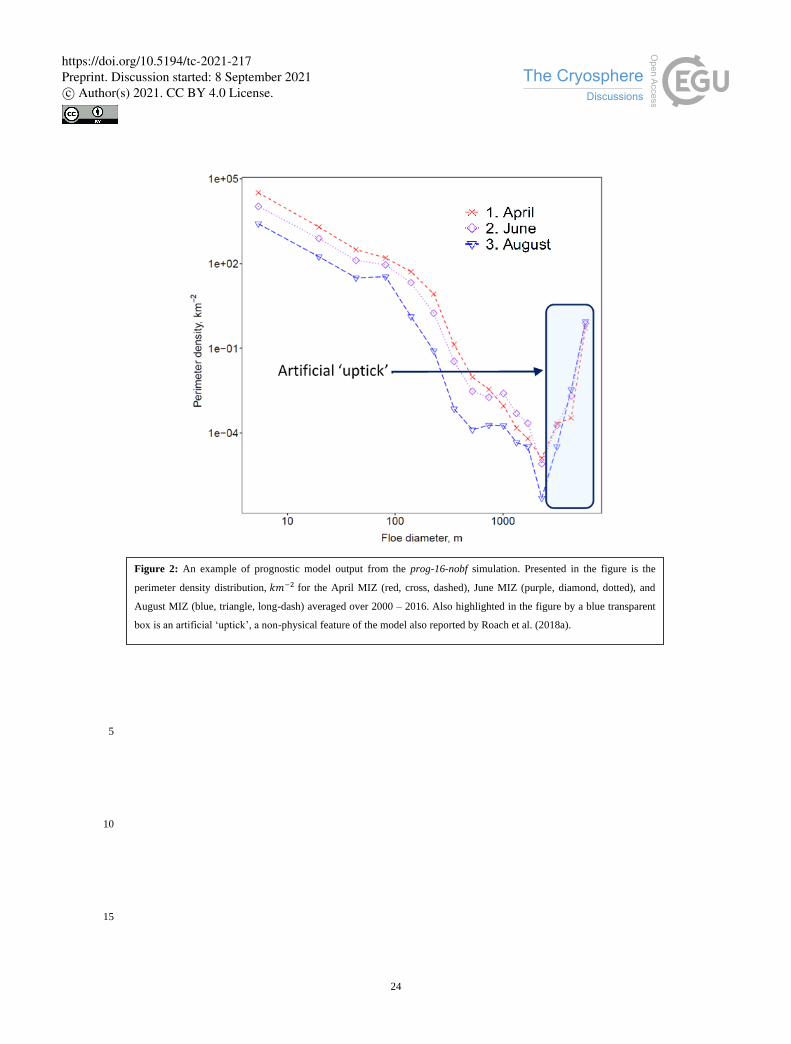
24

5

10

15

Figure 2: An example of prognostic model output from the prog-16-nobf simulation. Presented in the figure is the

perimeter density distribution, 𝑘𝑚−2 for the April MIZ (red, cross, dashed), June MIZ (purple, diamond, dotted), and

August MIZ (blue, triangle, long-dash) averaged over 2000 – 2016. Also highlighted in the figure by a blue transparent

box is an artificial ‘uptick’, a non-physical feature of the model also reported by Roach et al. (2018a).


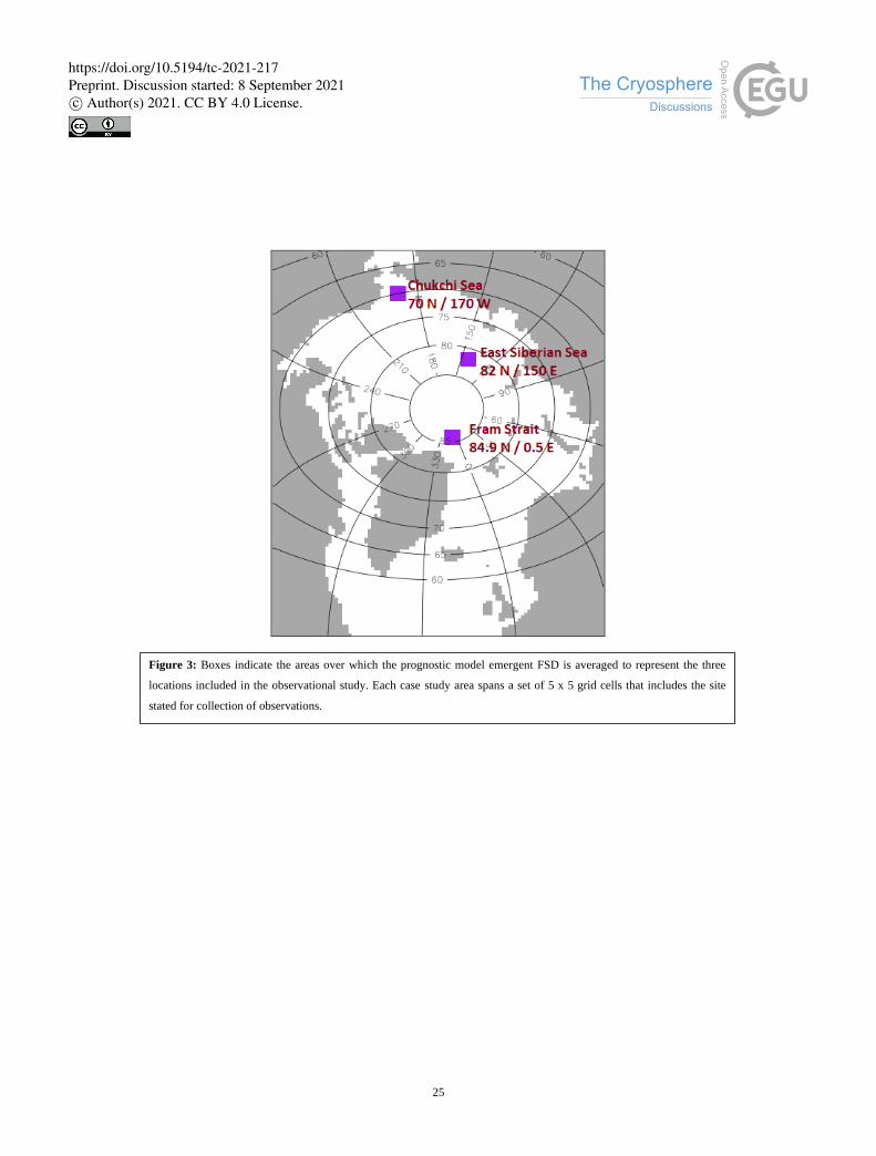
25

Figure 3: Boxes indicate the areas over which the prognostic model emergent FSD is averaged to represent the three

locations included in the observational study. Each case study area spans a set of 5 x 5 grid cells that includes the site

stated for collection of observations.


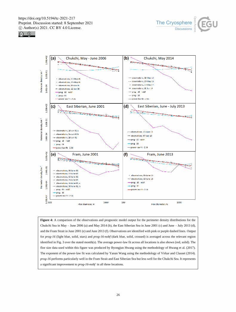
26

Figure 4: A comparison of the observations and prognostic model output for the perimeter density distributions for the

Chukchi Sea in May – June 2006 (a) and May 2014 (b), the East Siberian Sea in June 2001 (c) and June – July 2013 (d),

and the Fram Strait in June 2001 (e) and June 2013 (f). Observations are identified with pink or purple dashed lines. Output

for prog-16 (light blue, solid, stars) and prog-16-nobf (dark blue, solid, crossed) is averaged across the relevant region

identified in Fig. 3 over the stated month(s). The average power-law fit across all locations is also shown (red, solid). The

floe size data used within this figure was produced by Byongjun Hwang using the methodology of Hwang et al. (2017).

The exponent of the power-law fit was calculated by Yanan Wang using the methodology of Virkar and Clauset (2014).

prog-16 performs particularly well in the Fram Strait and East Siberian Sea but less well for the Chukchi Sea. It represents

a significant improvement to prog-16-nobf in all three locations.


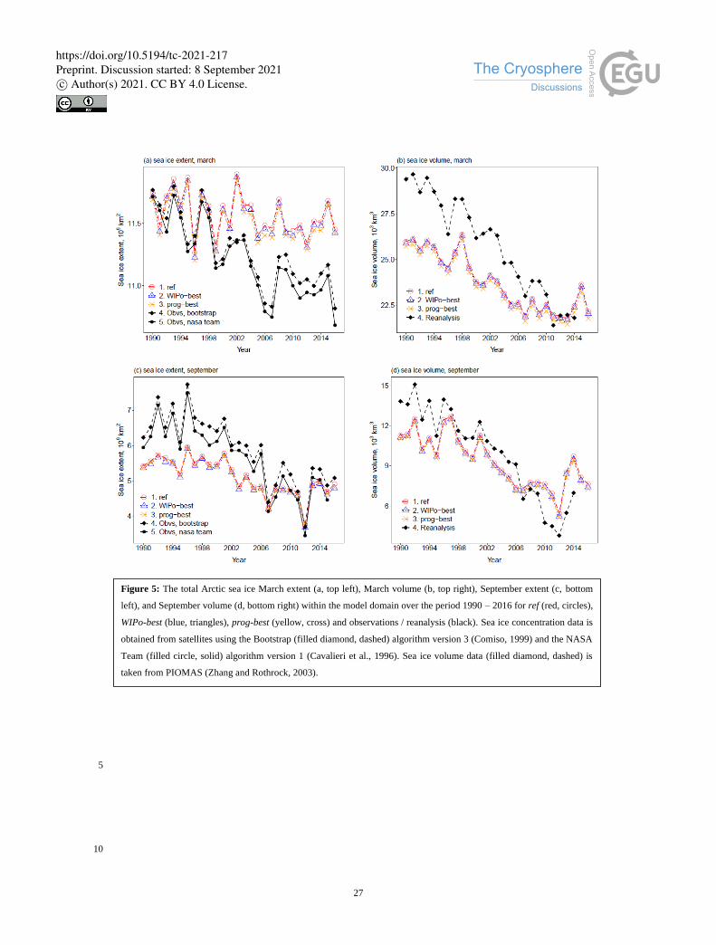
27

5

10

Figure 5: The total Arctic sea ice March extent (a, top left), March volume (b, top right), September extent (c, bottom

left), and September volume (d, bottom right) within the model domain over the period 1990 – 2016 for ref (red, circles),

WIPo-best (blue, triangles), prog-best (yellow, cross) and observations / reanalysis (black). Sea ice concentration data is

obtained from satellites using the Bootstrap (filled diamond, dashed) algorithm version 3 (Comiso, 1999) and the NASA

Team (filled circle, solid) algorithm version 1 (Cavalieri et al., 1996). Sea ice volume data (filled diamond, dashed) is

taken from PIOMAS (Zhang and Rothrock, 2003).


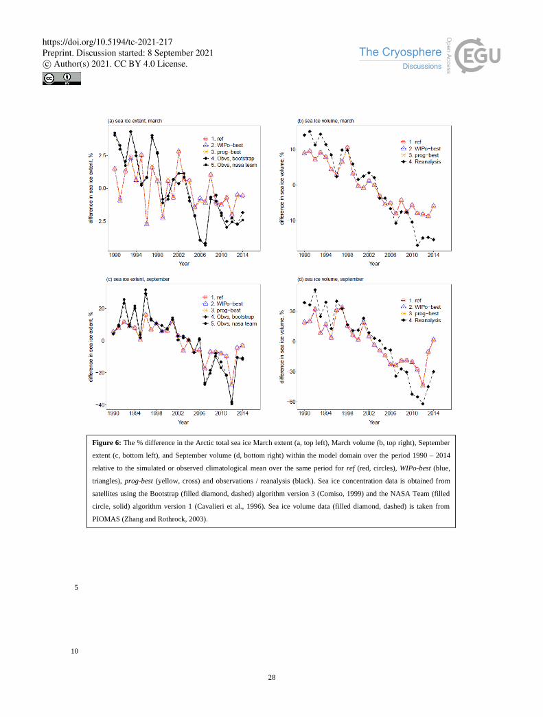
28

5

10

Figure 6: The % difference in the Arctic total sea ice March extent (a, top left), March volume (b, top right), September

extent (c, bottom left), and September volume (d, bottom right) within the model domain over the period 1990 – 2014

relative to the simulated or observed climatological mean over the same period for ref (red, circles), WIPo-best (blue,

triangles), prog-best (yellow, cross) and observations / reanalysis (black). Sea ice concentration data is obtained from

satellites using the Bootstrap (filled diamond, dashed) algorithm version 3 (Comiso, 1999) and the NASA Team (filled

circle, solid) algorithm version 1 (Cavalieri et al., 1996). Sea ice volume data (filled diamond, dashed) is taken from

PIOMAS (Zhang and Rothrock, 2003).


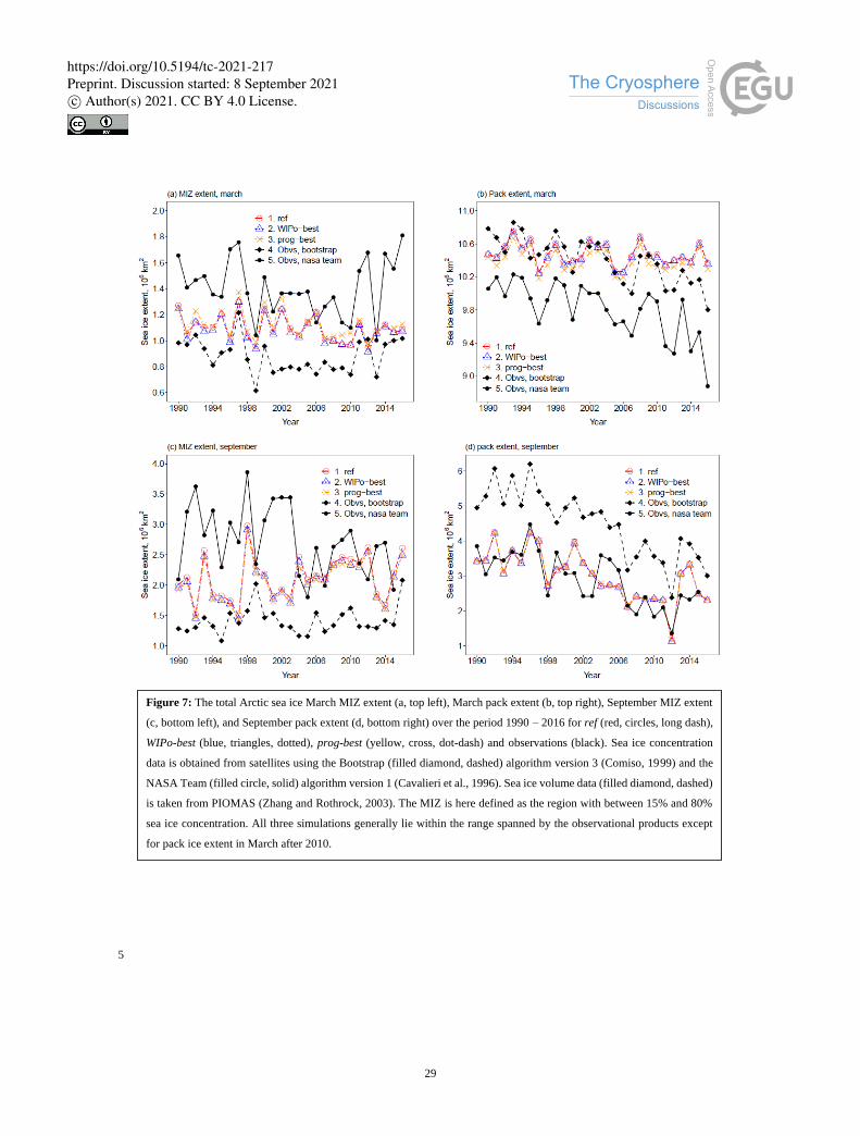
29

5

Figure 7: The total Arctic sea ice March MIZ extent (a, top left), March pack extent (b, top right), September MIZ extent

(c, bottom left), and September pack extent (d, bottom right) over the period 1990 – 2016 for ref (red, circles, long dash),

WIPo-best (blue, triangles, dotted), prog-best (yellow, cross, dot-dash) and observations (black). Sea ice concentration

data is obtained from satellites using the Bootstrap (filled diamond, dashed) algorithm version 3 (Comiso, 1999) and the

NASA Team (filled circle, solid) algorithm version 1 (Cavalieri et al., 1996). Sea ice volume data (filled diamond, dashed)

is taken from PIOMAS (Zhang and Rothrock, 2003). The MIZ is here defined as the region with between 15% and 80%

sea ice concentration. All three simulations generally lie within the range spanned by the observational products except

for pack ice extent in March after 2010.


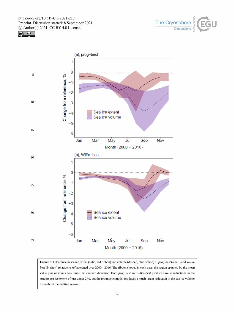
30

5

10

15

20

25

30

35

Figure 8: Difference in sea ice extent (solid, red ribbon) and volume (dashed, blue ribbon) of prog-best (a, left) and WIPo-

best (b, right) relative to ref averaged over 2000 - 2016. The ribbon shows, in each case, the region spanned by the mean

value plus or minus two times the standard deviation. Both prog-best and WIPo-best produce similar reductions in the

August sea ice extent of just under 2 %, but the prognostic model produces a much larger reduction in the sea ice volume

throughout the melting season.


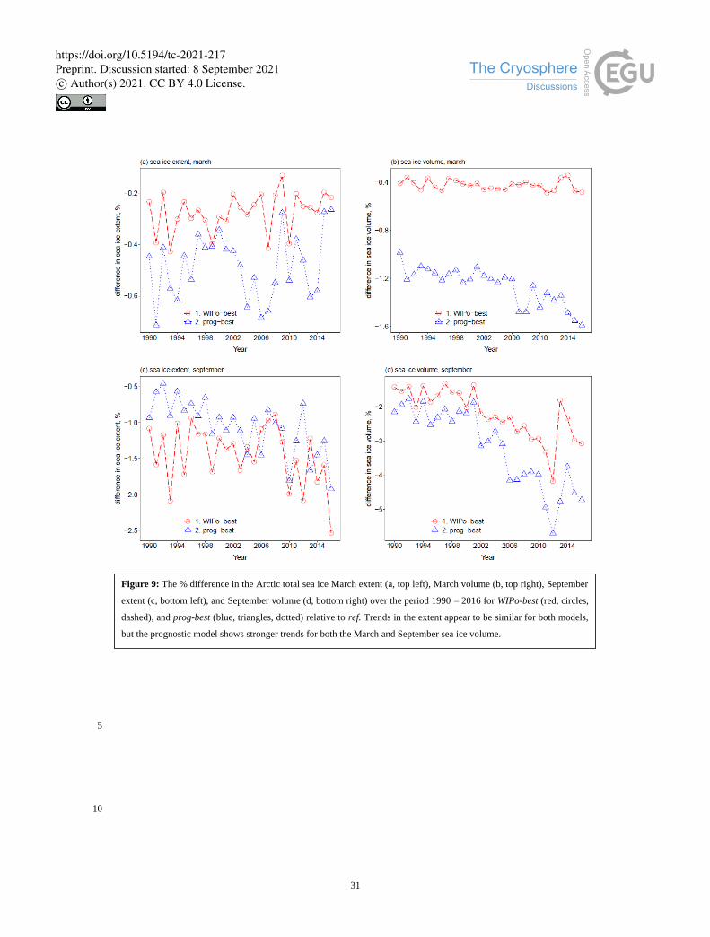
31

5

10

Figure 9: The % difference in the Arctic total sea ice March extent (a, top left), March volume (b, top right), September

extent (c, bottom left), and September volume (d, bottom right) over the period 1990 – 2016 for WIPo-best (red, circles,

dashed), and prog-best (blue, triangles, dotted) relative to ref. Trends in the extent appear to be similar for both models,

but the prognostic model shows stronger trends for both the March and September sea ice volume.


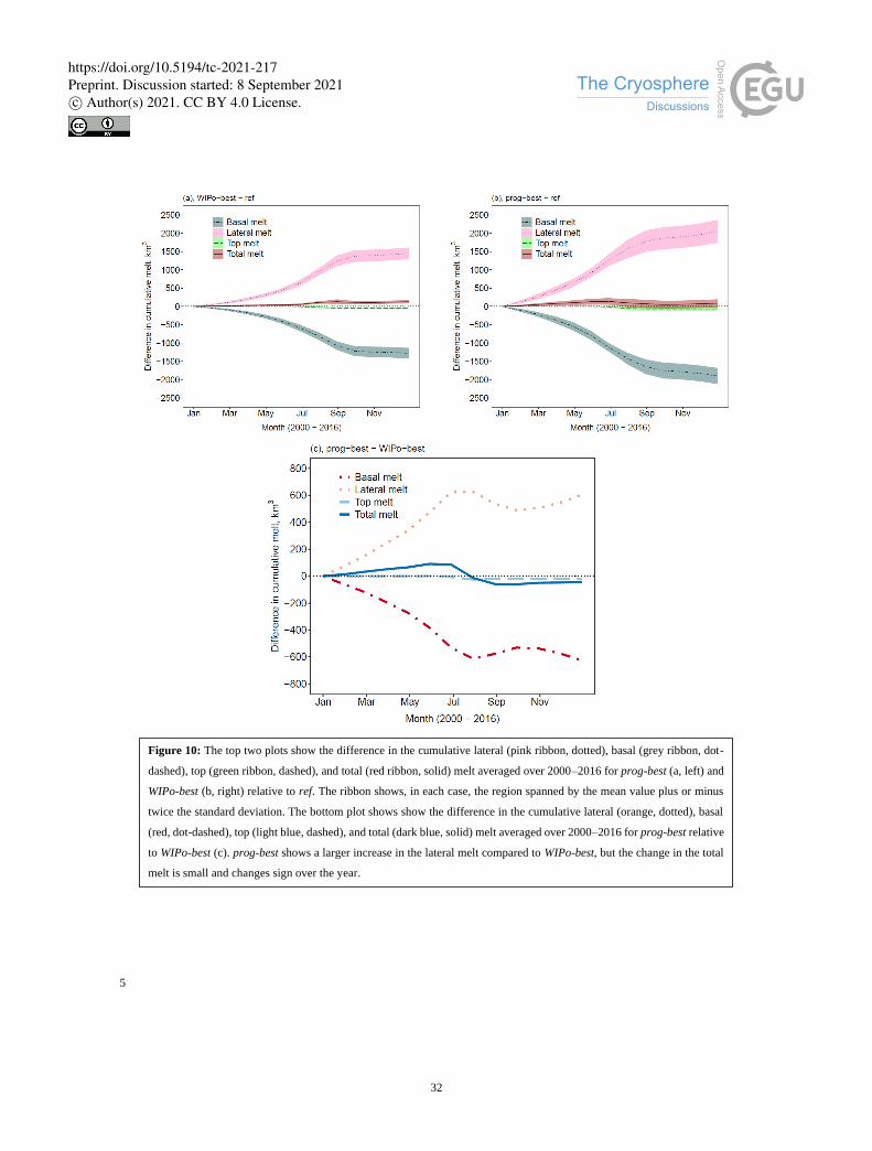
32

5

Figure 10: The top two plots show the difference in the cumulative lateral (pink ribbon, dotted), basal (grey ribbon, dot-

dashed), top (green ribbon, dashed), and total (red ribbon, solid) melt averaged over 2000–2016 for prog-best (a, left) and

WIPo-best (b, right) relative to ref. The ribbon shows, in each case, the region spanned by the mean value plus or minus

twice the standard deviation. The bottom plot shows show the difference in the cumulative lateral (orange, dotted), basal

(red, dot-dashed), top (light blue, dashed), and total (dark blue, solid) melt averaged over 2000–2016 for prog-best relative

to WIPo-best (c). prog-best shows a larger increase in the lateral melt compared to WIPo-best, but the change in the total

melt is small and changes sign over the year.


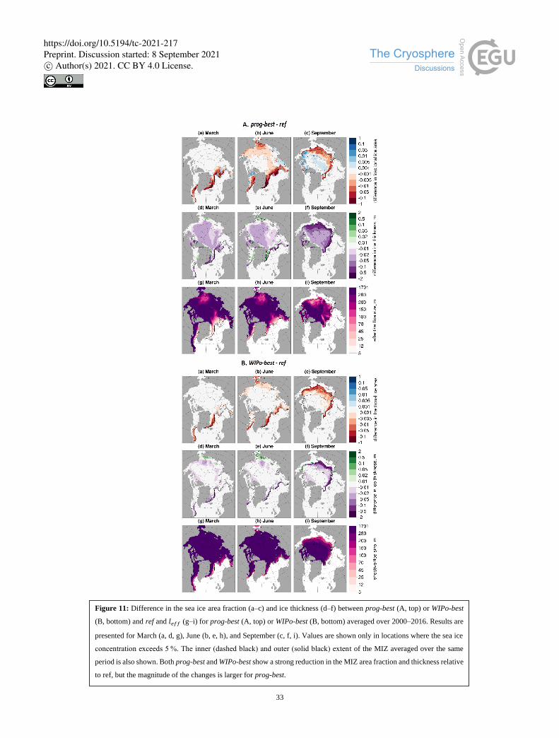
33

Figure 11: Difference in the sea ice area fraction (a–c) and ice thickness (d–f) between prog-best (A, top) or WIPo-best

(B, bottom) and ref and 𝑙𝑒𝑓𝑓 (g–i) for prog-best (A, top) or WIPo-best (B, bottom) averaged over 2000–2016. Results are

presented for March (a, d, g), June (b, e, h), and September (c, f, i). Values are shown only in locations where the sea ice

concentration exceeds 5 %. The inner (dashed black) and outer (solid black) extent of the MIZ averaged over the same

period is also shown. Both prog-best and WIPo-best show a strong reduction in the MIZ area fraction and thickness relative

to ref, but the magnitude of the changes is larger for prog-best.


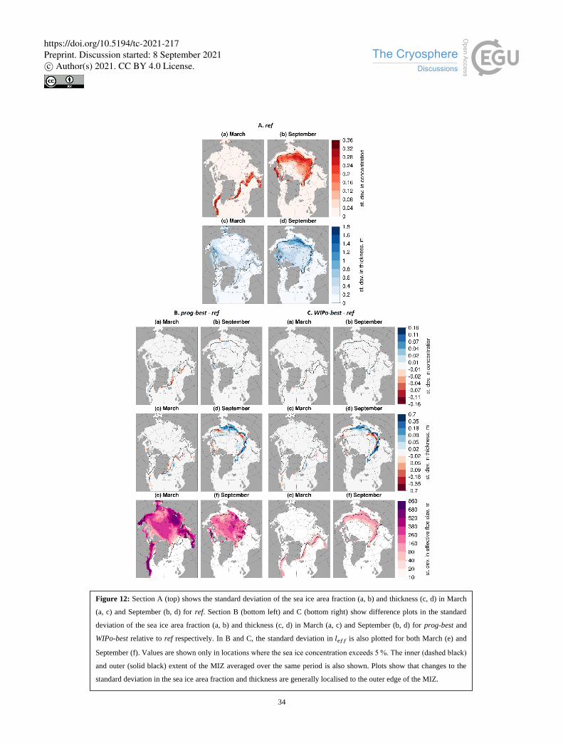
34

Figure 12: Section A (top) shows the standard deviation of the sea ice area fraction (a, b) and thickness (c, d) in March

(a, c) and September (b, d) for ref. Section B (bottom left) and C (bottom right) show difference plots in the standard

deviation of the sea ice area fraction (a, b) and thickness (c, d) in March (a, c) and September (b, d) for prog-best and

WIPo-best relative to ref respectively. In B and C, the standard deviation in 𝑙𝑒𝑓𝑓 is also plotted for both March (e) and

September (f). Values are shown only in locations where the sea ice concentration exceeds 5 %. The inner (dashed black)

and outer (solid black) extent of the MIZ averaged over the same period is also shown. Plots show that changes to the

standard deviation in the sea ice area fraction and thickness are generally localised to the outer edge of the MIZ.


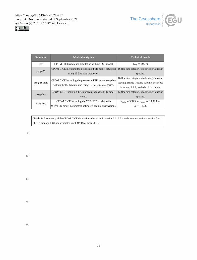
35

5

10

15

20

25

Simulation Model description Technical details

ref CPOM CICE reference simulation with no FSD model 𝑙𝑒𝑓𝑓 = 300 𝑚

prog-16 CPOM CICE including the prognostic FSD model setup but

using 16 floe size categories.

16 floe size categories following Gaussian

spacing.

prog-16-nobf CPOM CICE including the prognostic FSD model setup but

without brittle fracture and using 16 floe size categories.


spacing. Brittle fracture scheme, described

in section 2.2.2, excluded from model.

prog-best CPOM CICE including the standard prognostic FSD model

setup.


spacing.

WIPo-best CPOM CICE including the WIPoFSD model, with

WIPoFSD model parameters optimised against observations.

𝑑𝑚𝑖𝑛 = 5.375 𝑚, 𝑑𝑚𝑎𝑥 = 30,000 𝑚,

𝛼 = −2.56

Table 1: A summary of the CPOM CICE simulations described in section 3.1. All simulations are initiated sea ice free on

the 1st January 1980 and evaluated until 31st December 2016.


sea ice floe size: its impact on pan -arctic and local ice

Documents