SE-280Dr. Mark L. Hornick

1

Statistics Review

Linear Regression & Correlation

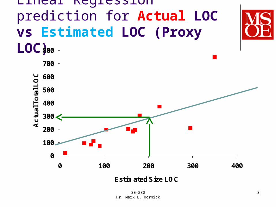
In subsequent labs, we’ll be predicting actual size or time using linear regression based on historical estimated size data from previous labs.

Note: this example showshistorical data for 13 labs

SE-280Dr. Mark L. Hornick

3

Linear Regression prediction for Actual LOC vs Estimated LOC (Proxy LOC)

0

100

200

300

400

500

600

700

800

0 100 200 300 400

Act

ual

To

tal L

OC

Estimated Size LOC

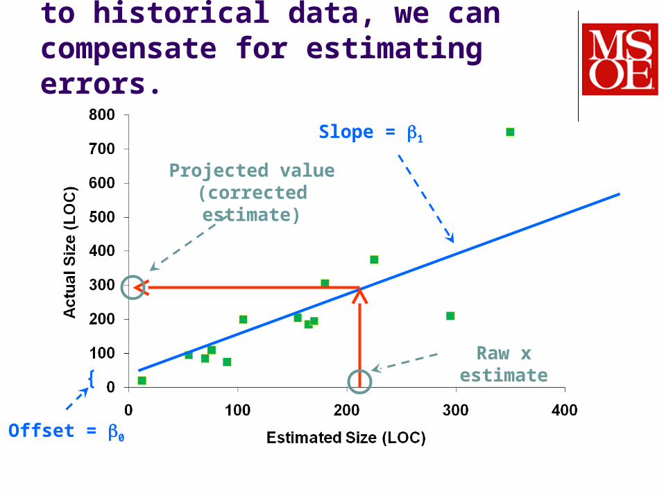
By fitting a regression line to historical data, we can compensate for estimating errors.

Slope = 1

Offset = 0

Projected value (corrected estimate)

Raw x estimate

To compute a new estimate, we use the regression line equation.

xest = raw estimateyproj = projected value (corrected estimate)

0 = offset of regression line1 = slope of regression line

estproj xy 10

These formulas are used to calculate the regression parameters.

xy

xnx

yxnyx

n

ii

n

iii

10

2

1

2

11

values actual previous of average

estimatesraw previous of average

points data previous of number

values actual previous

estimatesraw previous

y

x

n

y

x

i

i

SE-280Dr. Mark L. Hornick

7

Correlation (r) is a measure of the strength of linear relationship between two sets of variables

Value is +1 in the case of a (perfectly) increasing linear relationshipOr -1 in the case of a perfectly decreasing relationship

Some value in-between in all other cases Indicates the degree of linear dependence between the variables

The closer the coefficient is to either −1 or 1, the stronger the correlation between the variables

r > 0.7 is considered “good” for PSP planning purposes

After calculating the regression parameters ( values), we can also calculate the correlation coefficient.

To get the correlation coefficient (r), we first need to calculate r2.

With a single independent variable (x), we can get a signed correlation coefficient. In the general case, we only get the absolute value of the correlation coefficient (|r|); the "direction" of the correlation is determined by the sign of the "slope" value.

The correlation coefficient [0.0 to 1.0] is a measure of how well (high) or poorly (low) the historical data points fall on or near the regression line.

0.0

2.0

4.0

6.0

8.0

10.0

0 50 100 150 200 250 300 350

Let's look at an example of calculating the correlation.

For future reference, these data points come from test case 4 of lab 2.

0.0

2.0

4.0

6.0

8.0

10.0

0 50 100 150 200 250 300 350

We have already discussed how to calculate the regression parameters (beta values).

0 = 3.294671 = 0.01463

0.0

2.0

4.0

6.0

8.0

10.0

0 50 100 150 200 250 300 350

If we evaluate the regression line equation at each x value, we get the predicted y values.

ypred= 0.01463 x + 3.29467

0.0

2.0

4.0

6.0

8.0

10.0

0 50 100 150 200 250 300 350

To determine the correlation, we also need to calculate the mean y value (y).

y= 6.07(Mean of original y values)

0.0

2.0

4.0

6.0

8.0

10.0

0 50 100 150 200 250 300 350

Next, we need to sum the squares of two differences: (y – y) and (ypred – y).

y – y

ypred – y

Once we have the two sums, we can calculate the correlation coefficient.

2rr

n

ipredi

n

ipred

n

ii ii

yyyyyy1

2

1

2

1

2

Just in case you are curious, statisticians label the sum-square values like this:

Total sum of squares(variability) Sum of squares – predicted

(explained)

Sum of squares – error(unexplained)

One more time, where do the "ypred" values come from?

n

ii

n

ipred

yy

yyr

i

1

2

1

2

2

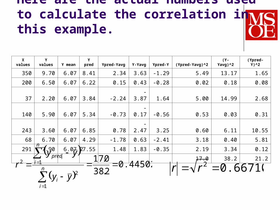
Here are the actual numbers used to calculate the correlation in this example.

n

ii

n

ipred

yy

yyr

i

1

2

1

2

2 0.445022.38

0.170.66710 2rr

X values Y values Y mean Y pred Ypred-Yavg Y-Yavg Ypred-Y (Ypred-Yavg)^2 (Y-Yavg)^2 (Ypred-Y)^2

350 9.70 6.07 8.41 2.34 3.63 -1.29 5.49 13.17 1.65

200 6.50 6.07 6.22 0.15 0.43 -0.28 0.02 0.18 0.08

37 2.20 6.07 3.84 -2.24 -3.87 1.64 5.00 14.99 2.68

140 5.90 6.07 5.34 -0.73 -0.17 -0.56 0.53 0.03 0.31

243 3.60 6.07 6.85 0.78 -2.47 3.25 0.60 6.11 10.55

68 6.70 6.07 4.29 -1.78 0.63 -2.41 3.18 0.40 5.81

291 7.90 6.07 7.55 1.48 1.83 -0.35 2.19 3.34 0.12

            17.0 38.2 21.2

SE-280Dr. Mark L. Hornick

16

We said we needed historical data to make predictions based on regression analysis

How do we know when it’s OK to use regression?

1. Quantity of data is satisfactory

We must have at least three points! It’s good to have a lot more 10 or more most recent projects are adequate

2. Quality of data is satisfactory

Data points must correlate (r2 0.5, |r| 0.707) The means that your process must be stable (repeatable)

SE-280Dr. Mark L. Hornick

17

We can also use linear regression to predict actual time.

Other examples on page 39.

0

0.5

1

1.5

2

2.5

3

3.5

0 50 100 150 200

Actual Size (LOC)

Act

ual

Tim

e (

hrs

)

0 1k ky x

xk

yk