screening for important factors in large-scale simulation models
DESCRIPTION
The present project discusses the application of screening techniques in large-scale simulation models with the purpose of determining whether this kind of procedures could be a substitute for or a complement to simulation-based optimization for bottleneck identification and improvement.Based on sensitivity analysis, the screening techniques consist in finding the most important factors in simulation models where there are many factors, in which presumably only a few or some of these factors are important. The screening technique selected to be studied in this project is Sequential Bifurcation. This method consists in grouping the potentially important factors, dividing the groups continuously depending on the response generated from the model of the system under study.The results confirm that the application of the Sequential Bifurcation method can considerably reduce the simulation time because of the number of simulations needed, which decreased compared with the optimization study. Furthermore, by introducing two-factor interactions in the metamodel, the results are more accurate and may even be as accurate as the results from optimization. On the other hand, it has been found that the application of Sequential Bifurcation could become a problem in terms of accuracy when there are many storage buffers in the decision variables list.Due to all of these reasons, the screening techniques cannot be a complete alternative to simulation-based optimization. However, as shown in some initial results, the combination of these two methods could yield a promising roadmap for future research, which is highly recommended by the authors of this project.TRANSCRIPT

Bachelor Degree Project in Automation Engineering Bachelor Level 30 ECTS Spring term 2015 Rafael Adrián García Martín José Manuel Gaspar Sánchez Supervisor: Amos H.C. Ng Examiner: Matías Urenda Moris
SCREENING FOR IMPORTANT FACTORS IN LARGE-SCALE SIMULATION MODELS: SOME INDUSTRIAL EXPERIMENTS

B S c i n A u t o m a t i o n E n g i n e e r i n g 1 5 A u g u s t 2 0 1 5

B S c i n A u t o m a t i o n E n g i n e e r i n g 1 5 A u g u s t 2 0 1 5
The University of Skövde
15 August 2015
The present report was written during the spring term of 2015 in a four-month project at the
University of Skövde. The research described herein was conducted under the supervision of
Professor Amos H.C. Ng and was examined by Matias Urenda Moris, Senior Lecturer and
Division Head of Production and Automation Engineering at this university.
All material in this thesis which is not the authors’ own work has been identified, and no
material is included for which a degree has previously been conferred on them.
Signed by,
The authors
Rafael Adrián García Martín José Manuel Gaspar Sánchez
[email protected] [email protected]
+34 665252386 +34 653247406
The supervisor The examiner
Amos H.C. Ng Matías Urenda Moris
Professor of Production & Automation Engineering Senior Lecture and Division head for Production and
Automation Engineering
[email protected] [email protected]
+46 500448541 +46 500448523

B S c i n A u t o m a t i o n E n g i n e e r i n g III | A b s t r a c t
An Abstract of
Abstract
Screening for important factors in large-scale simulation models: some industrial
experiments
by
García Martín, R. Adrián and Gaspar Sánchez, J. M.
Submitted to the School of Engineering Science in partial fulfillment of the requirements for
obtaining the Bachelor Degree in Automation Engineering
The University of Skövde
15 August 2015
The present project discusses the application of screening techniques in large-scale
simulation models with the purpose of determining whether this kind of procedures could be a
substitute for or a complement to simulation-based optimization for bottleneck identification
and improvement.
Based on sensitivity analysis, the screening techniques consist in finding the most important
factors in simulation models where there are many factors, in which presumably only a few or
some of these factors are important. The screening technique selected to be studied in this
project is Sequential Bifurcation. This method consists in grouping the potentially important
factors, dividing the groups continuously depending on the response generated from the
model of the system under study.
The results confirm that the application of the Sequential Bifurcation method can considerably
reduce the simulation time because of the number of simulations needed, which decreased
compared with the optimization study. Furthermore, by introducing two-factor interactions in
the metamodel, the results are more accurate and may even be as accurate as the results
from optimization. On the other hand, it has been found that the application of Sequential
Bifurcation could become a problem in terms of accuracy when there are many storage buffers
in the decision variables list.
Due to all of these reasons, the screening techniques cannot be a complete alternative to
simulation-based optimization. However, as shown in some initial results, the combination of
these two methods could yield a promising roadmap for future research, which is highly
recommended by the authors of this project.

B S c i n A u t o m a t i o n E n g i n e e r i n g IV | D e d i c a t i o n s
Dedications
To my family, my friends and my partner, without whom I would not be what I am.
Rafael Adrián
I would like to dedicate my work to my family and friends, who have been an indispensable
support. Special thanks to the exceptional people I met at Skövde.
José Manuel

B S c i n A u t o m a t i o n E n g i n e e r i n g V | A c k n o w l e d g e m e n t s
Acknowledgements
This project would not have been possible without the love, support, and encouragement I
received from my parents, my brother, my grandma and Natalia, my partner. I do not have
words to describe my deep gratitude for all they have provided me. I love you all.
Thanks to my friends, especially to Fernando, Marina, Manolo, Cristina, Sarai and Loli for
supporting me and sharing with me very many experiences. I am grateful to them for their
affection and their advice during my life.
Thanks also to Professor Amos H.C. Ng and Matias Urenda Moris, for their professionalism,
dedication and assistance with the present research.
Finally, thanks to José Manuel, for suffering me during this intense and wonderful year.
Rafael Adrián
I would like to show my gratitude to our supervisor, Amos H.C. Ng, for providing us all the help
required. His great vision when recommending us a topic and his knowledge gave us the
opportunity to work in this promising area.
I would also like to thank to Matias Urenda Moris, for his useful feedback, which turned our
research a success.
And final thanks to my project partner, Rafael Adrián, for his constant motivation.
José Manuel

Screening for important factors in large-scale simulation models: some industrial experiments
B S c i n A u t o m a t i o n E n g i n e e r i n g VI | C o n t e n t s
Table of Contents
ABSTRACT............................................................................................................................................ III
DEDICATIONS ......................................................................................................................................IV
ACKNOWLEDGEMENTS .......................................................................................................................V
TABLE OF CONTENTS ........................................................................................................................VI
LIST OF FIGURES ..............................................................................................................................VIII
LIST OF TABLES ..................................................................................................................................IX
1. INTRODUCTION ............................................................................................................................. 1
1.1. BACKGROUND TO THE STUDY, PROBLEM AND SIGNIFICANCE ......................................................... 1
1.2. AIM AND OBJECTIVES OF THE STUDY ........................................................................................... 2
1.3. METHODOLOGY AND REPORT STRUCTURE................................................................................... 3
1.4. LIMITATIONS AND DELIMITATIONS ................................................................................................ 4
1.5. SUSTAINABILITY ......................................................................................................................... 5
1.6. CONFIDENTIALITY ...................................................................................................................... 5
2. LITERATURE REVIEW .................................................................................................................. 6
2.1. SIMULATION FIELD ..................................................................................................................... 6
2.1.1. Discrete event simulation ................................................................................................ 6
2.1.2. Verification, validation and preparatory experiments ...................................................... 6
2.1.3. Simulation software ......................................................................................................... 7
2.2. SYSTEMS IMPROVEMENT VIA SIMULATION .................................................................................... 7
2.2.1. Design of experiments .................................................................................................... 7
2.2.2. Screening techniques ...................................................................................................... 7
2.2.3. Optimization .................................................................................................................... 8
2.3. SEQUENTIAL BIFURCATION ......................................................................................................... 9
2.3.1. Original Sequential Bifurcation ........................................................................................ 9
2.3.2. Sequential Bifurcation under uncertainty ...................................................................... 10
2.3.3. Controlled Sequential Bifurcation .................................................................................. 10
2.3.4. Two-Face Sequential Bifurcation .................................................................................. 10
2.4. SPLITTING INTO DIFFERENT GROUPS ......................................................................................... 11
2.5. CASE STUDIES RELATED TO SEQUENTIAL BIFURCATION ............................................................. 11
2.6. SUMMARY OF THE CHAPTER ..................................................................................................... 11
3. SEQUENTIAL BIFURCATION METHOD .................................................................................... 12
3.1. NOTATION ............................................................................................................................... 12
3.2. ASSUMPTIONS ......................................................................................................................... 12
3.3. EXPLANATION OF THE METHOD ................................................................................................. 13
3.4. UPPER LIMITS .......................................................................................................................... 14
3.5. SEQUENTIAL BIFURCATION CONSIDERING INTERACTIONS ........................................................... 14
3.5.1. Calculation of the interactions ....................................................................................... 14
3.5.2. Limitations when calculating the interactions ................................................................ 15
3.6. CONCLUDING REMARKS ........................................................................................................... 15
4. AUTOMATION OF THE METHOD ............................................................................................... 16
4.1. PROGRAMMING LANGUAGE SELECTED ...................................................................................... 16

Screening for important factors in large-scale simulation models: some industrial experiments
B S c i n A u t o m a t i o n E n g i n e e r i n g VII | C o n t e n t s
4.2. FLOWCHART OF THE COMPUTER PROGRAM ............................................................................... 16
4.3. PROGRAM STRUCTURE: MAIN FUNCTIONS .................................................................................. 17
4.3.1. Packages ....................................................................................................................... 17
4.3.2. Screening ...................................................................................................................... 17
4.3.3. Screening when considering interactions ..................................................................... 18
4.3.4. Simulate ........................................................................................................................ 19
4.3.5. Results .......................................................................................................................... 19
4.4. SUMMARY OF THE CHAPTER ..................................................................................................... 19
5. INDUSTRIAL SIMULATION MODELS ........................................................................................ 20
5.1. TABLE PRODUCTION SIMULATION MODEL (TPS) ........................................................................ 20
5.1.1. Steady state analysis: TPS ........................................................................................... 21
5.1.2. Replication analysis: TPS ............................................................................................. 21
5.2. VCC ASSEMBLY ...................................................................................................................... 22
5.2.1. Steady state analysis: VCC Assembly .......................................................................... 22
5.2.2. Replication analysis: VCC Assembly ............................................................................ 22
5.3. VCC L-FAB ............................................................................................................................. 23
5.3.1. Steady state analysis: VCC L-fab ................................................................................. 23
5.3.2. Replication analysis: VCC L-fab .................................................................................... 23
5.4. NBS ....................................................................................................................................... 24
5.4.1. Steady state analysis: NBS ........................................................................................... 24
5.4.2. Replication analysis: NBS ............................................................................................. 24
5.5. SUMMARY OF THE CHAPTER ..................................................................................................... 24
6. RESULTS ...................................................................................................................................... 25
6.1. TPS ....................................................................................................................................... 25
6.2. VCC ASSEMBLY ...................................................................................................................... 29
6.2.1. Sequential Bifurcation analysis: VCC Assembly ........................................................... 29
6.2.2. Comparison with the optimization study: VCC Assembly ............................................. 33
6.3. VCC L-FAB ............................................................................................................................. 34
6.3.1. Sequential Bifurcation analysis: VCC L-fab .................................................................. 34
6.3.2. Comparison with the optimization study: VCC L-fab ..................................................... 34
6.4. NBS ....................................................................................................................................... 38
6.4.1. Sequential Bifurcation analysis: NBS ............................................................................ 38
6.4.2. Comparison with the optimization study: NBS .............................................................. 38
6.5. SUMMARY OF THE RESULTS ...................................................................................................... 42
7. DISCUSSIONS.............................................................................................................................. 43
8. CONCLUSIONS ............................................................................................................................ 45
8.1. MAIN CONCLUSIONS ................................................................................................................. 45
8.2. FUTURE RESEARCH PROPOSED ................................................................................................ 46
REFERENCES ...................................................................................................................................... 47
APPENDIX ............................................................................................................................................ 49
APPENDIX A: LIST OF FORMULAS .......................................................................................................... 49
APPENDIX B: SB R-PROGRAM .............................................................................................................. 50

Screening for important factors in large-scale simulation models: some industrial experiments
B S c i n A u t o m a t i o n E n g i n e e r i n g VIII | F i g u r e s
List of figures
Figure 1. Work methodology followed in the project _______________________________________ 3
Figure 2. Sequential Bifurcation in relation to sustainability _________________________________ 5
Figure 3. MOO for systems improvement _______________________________________________ 9
Figure 4. SB applied to an Ericsson factory in Sweden ___________________________________ 10
Figure 5. Main techniques to find the most important factors in a simulation model _____________ 11
Figure 6. Explanation of the SB with a ten factors group __________________________________ 13
Figure 7. Flowchart of the program ___________________________________________________ 16
Figure 8. TPS model ______________________________________________________________ 20
Figure 9. Steady state of the TPS model ______________________________________________ 21
Figure 10. VCC Assembly model ____________________________________________________ 22
Figure 11. Steady state of the VCC Assembly model _____________________________________ 22
Figure 12. VCC L-fab model ________________________________________________________ 23
Figure 13. Steady state of the VCC L-fab model ________________________________________ 23
Figure 14. NBS model _____________________________________________________________ 24
Figure 15. Steady state of the NBS model _____________________________________________ 24
Figure 16. Most important factors of the TPS model without considering interactions ____________ 25
Figure 17. Most important factors of the TPS model when considering interactions _____________ 25
Figure 18. Pareto graphs of the TPS model ____________________________________________ 26
Figure 19. Most important interactions of the TPS model __________________________________ 27
Figure 20. Group bifurcations of the TPS model_________________________________________ 28
Figure 21. Most important factors of the VCC Assembly model without considering interactions ___ 29
Figure 22. Most important factors of the VCC Assembly model when considering interactions ____ 30
Figure 23. Pareto graphs of the VCC Assembly model ___________________________________ 31
Figure 24. Most important interactions of the VCC Assembly model _________________________ 32
Figure 25. Comparison of SB and optimization in the VCC Assembly model: Pareto graphs ______ 33
Figure 26. Comparison of SB and optimization in the VCC L-fab model: Pareto charts __________ 34
Figure 27. SB results of the VCC L-fab model __________________________________________ 35
Figure 28. Pareto graphs of the VCC L-fab model _______________________________________ 36
Figure 29. Most important interactions of the VCC L-fab model _____________________________ 37
Figure 30. Comparison of SB and optimization in the NBS model: Pareto graphs ______________ 38
Figure 31. SB results of the NBS model _______________________________________________ 39
Figure 32. Pareto graphs of the NBS model ____________________________________________ 40
Figure 33. Most important interactions of the NBS model _________________________________ 41
Figure 34. Buffers’ influence in the SB: TPS model example _______________________________ 43
Figure 35. Incongruence of the results: An experiment with the TPS model ___________________ 44
Figure 36. Combination of SB and optimization: initial results ______________________________ 44

Screening for important factors in large-scale simulation models: some industrial experiments
B S c i n A u t o m a t i o n E n g i n e e r i n g IX | T a b l e s
List of tables
Table 1. Replication analysis of the TPS model _____________________________________ 21
Table 2. Replication analysis of the VCC Assembly model _____________________________ 22
Table 3. Replication analysis of the VCC L-fab model ________________________________ 23
Table 4. Replication analysis of the NBS model _____________________________________ 24
Table 5. Simulations required by SBO, SB and SBi to find the most important factors ___________ 42

Screening for important factors in large-scale simulation models: some industrial experiments
B S c i n A u t o m a t i o n E n g i n e e r i n g 1 | P a g e
1. INTRODUCTION
Background to the study, aim and objectives, report structure, limitations,
sustainability and confidentiality
In the present project, the Sequential Bifurcation method (SB), one type of screening for
important factors in large-scale simulation models, is studied and analyzed by performing
some experiments in order to compare its results with the optimization study of different
industrial models.
The screening technique studied in this project is the original SB presented by Bettonvil and
Kleijnen (1996), which is applied in an automated manner to four discrete event simulation
models: one of these models serves as an explanation of the method, whereas the others
three are used to compare simulation-based optimization (SBO) and Sequential Bifurcation.
1.1. Background to the study, problem and significance
The detecting of important factors in industrial systems is necessary to identify the required
changes to perform, e.g. availability of the machines or capacity of the warehouses, with the
purpose of improving these systems in terms of throughput, work-in-progress (WIP) or lead
time, among other parameters. In this sense, simulation is an effective method to reach this
objective and generally for the analysis of large-scale, complex, real-world or artificial systems.
Nowadays, there are many techniques that can be applied to simulation models with the aim
of finding their most important factors. Among them, design of experiments and simulation-
based optimization are the most well-known ones, even though SBO, which can be defined
as finding the best input variables, i.e. the most important factors in this context, among all the
possible variable combinations without explicitly evaluating each possibility (Carson & Anu,
1997), is the current method used because of its accuracy.
The problem arises when there are a large number of factors that can be subject to changes
in a simulation model. When it happens, the search space in an optimization study increases
exponentially. Take a simple example: for a 2-level full factorial study, the combination of 10
variables is 210=1024. Nevertheless, if the number of factors is increased by ten times to 100,
then the total number of possible combinations is 1.27x1030, which makes any enumeration
impossible. The problem is even worse in terms of time: due to the complexity of the models,
each simulation takes a relatively long time; consequently, and since the search space is
higher, the time required to find the most important factors using optimization is extremely long
comparing with other techniques. For this reason, simulation models with many factors would
pose a difficult challenge to a simulation-based optimization study.
In the literature, a common method to ameliorate this problem is screening, a type of design
of experiments. By using the screening techniques, and more precisely, Sequential
Bifurcation, which is particularly suitable for large-scale simulation models, fewer simulations
are required to find the most important factors in a simulation model, reducing the time of the
study significantly. However, the reliability of the SB is under discussion (Kleijnen, et al., 2006),
especially in terms of accuracy. Therefore, it is necessary to perform a comparison between
Sequential Bifurcation and simulation-based optimization in order to test the precision of the
procedure.

Screening for important factors in large-scale simulation models: some industrial experiments
B S c i n A u t o m a t i o n E n g i n e e r i n g 2 | P a g e
1.2. Aim and objectives of the study
The purpose of the present project is to apply the Sequential Bifurcation method in different
industrial models in order to determine whether the screening techniques could be a substitute
for or a complement to the current method that is based on stochastic evolutionary
optimization.
In order to reach the aim, the following objectives have to be achieved:
1. Understand and describe the Sequential Bifurcation method.
A proper study of the method is fundamental to make a correct implementation. Therefore,
a concomitant objective is to perform a literature review, necessary to summarize and
study the different variants of the original procedure.
2. Develop a computer program for the application of the Sequential Bifurcation method.
The program should show the results of the screening method in terms of time, number of
simulations and most important factors in the four discrete event simulation models to
study. It should be emphasized that the program needs to be combined with FACTS
Analyzer, simulation software developed at the University of Skövde, to run the simulations.
This is because the models studied in this project were built under this program.
Furthermore, other sub-objectives are proposed with regards to the development of the
computer program, such as:
2.1. Create the code for the method, structuring it into different functions.
2.2. Show the Sequential Bifurcation results using different charts, similarly to the one
shown in the publication presented by Kleijnen, Bettonvil and Persson (2006).
2.3. Develop the code to calculate a Pareto chart based on the results of the
corresponding simulation models, both of Sequential Bifurcation and simulation-
based optimization.
This objective and their corresponding sub-objectives represent the key part of the project;
the proper accomplishment of the aim of this thesis depends on its consecution.
3. Analyze the reliability of the Sequential Bifurcation method.
This objective is especially related to the aim of the project, although it could be executed
without any comparison with optimization. Notwithstanding, without this comparison the
validation of the results would be more difficult to achieve. Thus, after finishing the
automation of the method and the experiments, the reliability of the SB should be discussed
based on the results obtained directly from the method and especially from the comparison
with the optimization study.
Furthermore, the problems found during the project should be explained with the purpose of
creating a roadmap for future researchers.

Screening for important factors in large-scale simulation models: some industrial experiments
B S c i n A u t o m a t i o n E n g i n e e r i n g 3 | P a g e
1.3. Methodology and report structure
In order to achieve the goals presented in this project properly, a work methodology based on
different steps needs to be follow. The flowchart shown in figure 1 represents the stages to do
during the project with their corresponding chapters in the report.
First of all, it is essential to perform a literature review with the objective of analyzing the results
obtained in previous research of this field as well as to summarize the different variants of the
Sequential Bifurcation method that have been studied previously.
Once the different types of screening methods are studied, the Sequential Bifurcation method
is described and analyzed, basing especially on the 1996 and 2006 Sequential Bifurcation
publications co-authored by Professor Kleijnen.
After that, the automation of the method starts. It is the most difficult and time-consuming task
of the project. The experiments are done while developing the code and the results obtained
are used as feedback to check the correctness of the implementation. The final results are
achieved through several revisions and improvements of the code.
As a final point, the comparison with the optimization study is performed in order to contrast
the accuracy of the Sequential Bifurcation method with the simulation-based optimization.
Additionally, the conclusions need to be drawn based on the results obtained from the
experiments and also from the comparison with the optimization study.
Regarding the report structure, it is divided into eight chapters, following the same organization
as the methodology.
Figure 1. Work methodology followed in the project. Source: own elaboration
Fee
db
ackDeveloping of
the code4Ch.
Experiments
6Ch. 5
Understanding of the method 3
Literature study 2Ch.
Ch.
Analysis of the results 8Ch. 7
Screening for important factors in large-scale simulation models: some industrial experiments
B S c i n A u t o m a t i o n E n g i n e e r i n g 4 | P a g e
1.4. Limitations and delimitations
The present project has some influences that cannot be controlled. The following limitations
are the most significant ones:
1. Simulations require a specific software.
Since the models to study are built in FACTS Analyzer, this program is required to perform
the simulations. More precisely, an executable, xsim-runner.exe, is needed to perform the
experiments. This file is called with a specific code, as is shown in chapter 4.
This limitation represents a potential weakness in the project. All the simulations depend
on this program, which is updated and controlled by the University of Skövde.
2. High-performance computers are required for the simulations.
This is a limitation especially related to time. Depending on the complexity of the model to
study, a complete experiment could spent more or less time so that this is an important
variable to take into account. In this sense, many parts of the SB computer program require
a lot of resources in terms of computer performance, such as the computing of the
interactions or the calculation of the graphs.
3. The factors to study are decided by the provider of the models.
The majority of the models of this project have a huge amount of factors, although not all
of them are studied in the SB implementation. The provider of the models determines
beforehand the factors to study, which entails a limitation especially in terms of flexibility.
4. Likewise, the time-limit for the realization of the project represents a significant limitation.
Regarding the delimitations, there are some boundaries set in this project that have to be
mentioned:
1. The output variable to study is the throughput (TH).
Even though the SB program is devised to study the TH, WIP and lead time, only the
throughput is studied in the experiments because the original SB implementation analyses
the factors in terms of TH, and also for the time consumed to study the other parameters.
2. Only the interactions among the first ten most important factors are calculated.
The majority of the simulation models does not have more than ten relevant main effects
(see chapter 3). Based on the assumption explained in this chapter, the rest of the
interactions are not significant.
3. The minimum number of replications is set to 5.
The statistics studies argue that this is the minimum number of replications needed in a
simulation experiment to obtain credible results. However, it could be insufficient (Hoad, et
al., 2007), hence a replication analysis needs to be performed to each model.
4. The scope of the project is limited to the implementation and analysis of the existing
Sequential Bifurcation method, i.e. it does not include the development of any new
screening method.

Screening for important factors in large-scale simulation models: some industrial experiments
B S c i n A u t o m a t i o n E n g i n e e r i n g 5 | P a g e
1.5. Sustainability
Sustainability can be defined as “the successful management of resources to satisfy human
needs while maintaining and enhancing the quality of the environment and conserving
resources” (Hietala-Koivu, 1999). In this context, gearing the companies’ activities toward
sustainable development is a necessary task nowadays.
The sustainability of the enterprises depends on the efficiency of their processes. Today, the
complexity of the systems has been increased due to the technological development.
Therefore, simulating these processes has become an important task to understand the
behavior of the systems and also to improve their efficiency.
The main objective of the SB is to find the important factors in a simulation model; thus, the
efficiency of the system can be improved, decreasing the number of changes to implement.
Additionally, finding the most important factors in the system can indirectly reduce any
environmental impact, e.g. due to adding unnecessary resources.
Furthermore, the SB method can be applied to different types of models. Even though in this
research all the models are related to the industry, the Sequential Bifurcation method can
improve sustainability if the models consider environmental factors, as in the models studied
by Bettonvil and Kleijnen in 1996. Figure 2 represents the main aspects of the sustainability
in the simulation field and its relationship with Sequential Bifurcation.
Figure 2. Sequential Bifurcation in relation to sustainability. Source: own elaboration
1.6. Confidentiality
The present project was realized at the University of Skövde, without any enterprise
cooperation. Hence, no confidentiality document was required to be signed. However, some
aspects regarding the privacy have been considered because many real industrial models
were used during the project. The names of the factories, details of the companies and real
data of the simulation models used in the study have not been explicitly revealed. All the data
that could be thoroughly discussed, as throughput results, has not been included in this report,
especially in the charts and final results.
SB
Business
Process Simulation
Most Important Factors

Screening for important factors in large-scale simulation models: some industrial experiments
B S c i n A u t o m a t i o n E n g i n e e r i n g 6 | P a g e
2. LITERATURE REVIEW
Review of the simulation literature and the progress and development of the SB
In this heading of the project, a deep review of the simulation literature is shown in order to
relate the progress of this field with the Sequential Bifurcation method, as well as to make
know the different variants of this technique that have been studied previously. Furthermore,
some real case studies related to Sequential Bifurcation are explained.
2.1. Simulation field
Simulation is the process of designing a model of a system with which experiments are
performed to understand the operating of that system or evaluate different strategies
(Shannon, 1976). This tool is usually used to predict situations and gather information before
implementing changes in real systems.
2.1.1. Discrete event simulation
Nowadays, the majority of the real systems are too complex to be modeled by using analytical
techniques (Ng, et al., 2008). Hence, one of the key points when doing a simulation study is
the type of simulation modeling to use. Discrete event simulation (DES) is the common one in
this area because it “provides an intuitive and flexible approach to representing complex
systems” (Karnon, et al., 2012). The main characteristic of DES is that it considers the
operating of the systems as a set of discrete events, which facilitate the simulation process.
In this project, and as mentioned before, the experiments are performed with DES models.
2.1.2. Verification, validation and preparatory experiments
The verification and the validation of the models are very important aspects that have to be
taken into account when starting a simulation study.
Once the model is finished, it is important to determine whether the model has been correctly
built into the simulation software, i.e. to start a debugging process (Law, 2003). This is called
verification. Afterward, it is necessary to make a validation process; it represents the
comparison between the model built and the real system with the purpose of determining the
accuracy of its representation and also to reduce or eliminate the variability of that system
(Law, 2009). In this research, it has been assumed that the models provided have been
verified and validated beforehand. No verification and validation process has been made.
Another aspect to be considered in a simulation study are the preparatory experiments. Both
a steady-state and replication analysis must be made to validate the results. A steady-state
study determines the time that a system requires to be stable (Mahajan & Ingalls, 2004) and
it is usually the experience of the researchers which determines the correct value. Regarding
the replication analysis, the majority of the authors argues about the minimum number of
replications necessary in a simulation experiment: despite the fact that statistics determines
that at least is five, this number is currently under discussion.
These experiments are crucial to improving the accuracy of a simulation study because the
data collection must be performed under steady state and with the correct number of
replications. In the present project, a replication analysis sheet provided by the University of
Skövde has been used for the preparatory experiments.

Screening for important factors in large-scale simulation models: some industrial experiments
B S c i n A u t o m a t i o n E n g i n e e r i n g 7 | P a g e
2.1.3. Simulation software
Attention should also be drawn when choosing a simulation software. Nowadays, there are
many options that could be considered before starting a simulation project. Some of them are
well-known, such as Arena or Plant Simulation, while others are specific for some companies
or universities. Since the models studied in the present project were built in FACTS Analyzer,
all the simulations have been performed using this program. However, its interface has not
been used because the SB calls its simulator, xsim-runner, automatically.
Additionally, FACTS Analyzer offers different optimization tools whose results have been used
in this project to compare with the ranking of the most important factors obtained from the
Sequential Bifurcation method.
2.2. Systems improvement via simulation
There are many techniques, as stated previously, that can be applied to discrete event
simulation models with the aim of improving the systems. Among them, design of experiments
and simulation-based optimization are the most important ones.
2.2.1. Design of experiments
The number of factors in a simulation model is in accordance with the complexity of the system
that it represents. Related to this, design of experiments, a set of techniques based on
sensitivity analysis, has the objective of finding the most important factors by making the least
amount of simulations. Thus, there are different strategies that can be applied. The most
important ones are: one-factor-at-a-time, 2k factorial design and 2k-p fractional factorial design
(Law, 2014), where k is the number of factors and p depends on the experimental design.
One-factor-at-a-time makes simulations at two different values of an input factor while keeping
the rest of the factors at a fixed value. This procedure is inefficient in terms of simulations and
it assumes that there are no interactions in the metamodel.
One way to calculate these interactions is by using a 2k factorial design, choosing two levels
for each factor and calculating all the 2k possible inputs combinations. This technique is much
more accurate than the one-factor-at-a-time technique when there are interactions between
the factors of the model. It is also more time-demanding in terms of simulations required.
Finally, the 2k-p fractional factorial design makes possible to estimate the main effects and the
two-factor interactions with a reduced amount of simulations. The time required decreases
while increasing the value of p. However, the accuracy of the calculations decreases as well.
On the other hand, quadratic effects can be estimated in many of these methods. In this case,
k extra runs are needed and each factor has to be simulated for more than two values
(Kleijnen, 1998).
2.2.2. Screening techniques
Screening techniques are a type of design of experiments. They can be defined as a group of
methods whose objective is to find the factors for which a small variation of the inputs implies
an improvement in the output of the system. These techniques assume that the response of
the model depends only on a few factors, which is called the principle of parsimony.

Screening for important factors in large-scale simulation models: some industrial experiments
B S c i n A u t o m a t i o n E n g i n e e r i n g 8 | P a g e
Several screening techniques have been developed over the last decade. Among them, it is
possible to emphasize the next ones: supersaturated design, group screening, multiple group
screening or Sequential Bifurcation, among others (Dupuy, et al., 2014).
A supersaturated design uses fewer runs than the number of factors to study; it was developed
by Satterthwaite (1959) as cited by Dupuy et al. (2014). Afterward, many different methods
were created in this field, like the one published by Watson (1961), based on Dorfman’s
publications (1943). This method, called group screening, starts combining the factors into
small groups that are treated as a single factor. The aim of this procedure is to use a simpler
design to study the system.
A different important variant of this method is called multiple group screening (Morris, 1987).
This method assigns each factor to more than one group. After making the necessary
simulations, a factor is defined as potentially influential if all groups that contain this factor are
active.
Finally, Sequential Bifurcation is a group-screening technique published by (Bettonvil &
Kleijnen, 1996). This method and its different variants are explained in section 2.3.
2.2.3. Optimization
According to Carson and Anu (1997), and as stated before, simulation-based optimization is
“the process of finding the best input variable values from among all possibilities without
explicitly evaluating each possibility”, whose goal is to maximize the information obtained in a
simulation experiment while reducing the resources spent.
Thus, the current optimization method, based on stochastic evolutionary optimization, is
commonly used in the simulation field because of the accuracy of its results, especially for
bottleneck identification and improvement (Ng, et al., 2014).
On the other hand, it should be noted the difficulty when optimizing a system, which depends
especially on the number of input parameters. In this sense, the major problem of optimization
is that by using this method it is not possible to conclude with assurance that one configuration
is the best one among all the possibilities. This is because the optimization method does not
study all the inputs combinations.
In this context, many researchers have been focused on designing an evaluation of different
algorithmic, as did Riley in her study (2013). More precisely, this author discussed and
reviewed theoretically the discrete-event simulation optimization methodology, proposing
areas of study for future research, such us designing intelligent optimization interfaces or
dynamically-integrated optimization software.
Another of the aspect to empathize in regards to optimization is the possibility of applying
multi-objectives into the experiments. In their study, Amos, Pehrsson and Bernedixen (2014),
show the benefits of implementing multi-objective optimization (MOO) in a simulation
experiment. Figure 3 shows the concept of using MOO for bottleneck analysis, in which the
TH is intended to be maximized while minimizing the number of changes.

Screening for important factors in large-scale simulation models: some industrial experiments
B S c i n A u t o m a t i o n E n g i n e e r i n g 9 | P a g e
It is possible to observe in the picture below (see figure 3) the multi-objectives proposed: f1(x)
represents the TH to be increased and f2(x), the number of changes to be minimized.
Moreover, TH0 is the throughput without implementing any change; THmax, the maximum
throughput to be reached by the system when implementing Cmax changes, which represents
the maximum number of changes to perform in order to obtain that TH, meaning that if more
than Cmax changes were implemented, f2(x) > Cmax, the TH will be the same. They call these
outcomes as inferior solutions. Finally, THt represents the throughput when implementing a
determined number of changes, lower than Cmax.
Figure 3. MOO for systems improvement. Source: Ng et al. (2014)
Based on their results, it is possible to conclude that MOO is a powerful tool to use in
simulation studies, in the sense that the optimal combinations are generated in a single
optimization run.
2.3. Sequential Bifurcation
The present project focuses on the Sequential Bifurcation method. Here follows a deeper
analysis of this method and its different variants developed.
2.3.1. Original Sequential Bifurcation
Sequential Bifurcation origins in 1996, when Bettonvil and Kleijnen published a report
explaining the method and applying it to a model. The aim of this method is to find the most
important factors (k) among the great many (K) in large-scale models, reducing the number of
simulations required (n), where k<<K and n<<K.
Moreover, the authors also extended their study considering two-factor interactions, which
makes the metamodel more precise. With this metamodel, it is possible to estimate whether
the interactions are important or not, although its value cannot be calculated.

Screening for important factors in large-scale simulation models: some industrial experiments
B S c i n A u t o m a t i o n E n g i n e e r i n g 10 | P a g e
Ten years later, Kleijnen, Bettonvil and Persson (2006) explained, applied, and discussed the
SB. They showed graphically its behavior in a case study with different models from an
Ericsson factory in Sweden, as shown in figure 4. In this picture, it is possible to observe the
division of the factors in their experiment.
Figure 4. SB applied to an Ericsson factory in Sweden. Source: Kleijnen et al. (2006)
2.3.2. Sequential Bifurcation under uncertainty
The method created by Bettonvil and Kleijnen was developed for deterministic simulations,
which is appropriate only in a few cases. In this context, there were many authors who tried to
improve the original method, e.g. Cheng (1997). This author extended the original SB, naming
it as SB-under-uncertainty (SBU). The aim of this method is to apply the SB to models whose
response is stochastic and subject to significant error, maintaining the flexibility instead of
reaching a precise level of significance.
2.3.3. Controlled Sequential Bifurcation
Another important variant of Sequential Bifurcation is Controlled Sequential Bifurcation (Wan,
et al., 2003). The Controlled Sequential Bifurcation procedure (CSB) contains the main
concepts from the original SB and the SBU method. The CSB controls with several algorithmic
the correctness of the results with the objective of determining more precisely its importance.
2.3.4. Two-Face Sequential Bifurcation
Sequential Bifurcation requires the user to establish the direction of the effect of each factor.
This can be a problematic step because if there were any mistakes, the results could be
completely different. Sanchez, Thomas and Wan (2005), tried to solve this problem by
developing the Two-Face Controlled Sequential Bifurcation method, FF-CSB. It consists of
two different phases when the screening is performed: firstly, the signs and magnitudes of the
effects are calculated; secondly, these results are used to apply CSB.
It has to be emphasized that the original SB is the variant implemented in the present project
although many of the aspects of the other variants are included in the study, e.g. the inclusion
of stochastic models or assuring the correctness of the results by applying several preparatory
experiments. Furthermore, and since the aim of the project is to compare the screening
techniques with SBO, the selection of one type of another would not affect to the validation of
the results.

Screening for important factors in large-scale simulation models: some industrial experiments
B S c i n A u t o m a t i o n E n g i n e e r i n g 11 | P a g e
2.4. Splitting into different groups
One of the key elements in a Sequential Bifurcation procedure is the way of splitting the group
of factors. Frazier and Li Chen (2012) studied the optimal group-splitting problem using a
Bayesian-dynamic programming method. They introduced the SB and formulated the optimal
group splitting problem analyzing two different versions.
The first case studied in their article assumed that the probability of having an important factor
was homogeneously distributed. In this circumstance, the conclusion was that dividing a group
in half is the optimal decision when the number of factors is a power of two, consistent with
the rule used by Bettonvil and Kleijnen (1996). The second case had two types of factors: one
with a high probability of importance and a second one with a low probability of importance. In
this circumstance, the optimal solution is to divide based on the category of the factors.
2.5. Case studies related to Sequential Bifurcation
There are many case studies in the field of screening and, more precisely, related to
Sequential Bifurcation. Two of them are explained next.
Yaesoubi and Roberts (2007) applied screening techniques in a medical simulation model for
colorectal cancer to find the most important factors. By performing the experiment, they found
that, out of the 72 factors considered, only 8 seemed to be important. The system was driven
by a short list of factors although many others had a contribution.
In a closer relation with Sequential Bifurcation, Shi, Shang, Liu and Zuo (2014) applied this
method in a supply chain for JIT operations. In this case, the results were also significant,
finding three important factors out of the 58 considered with a fewer number of simulations.
The Sequential Bifurcation method that they applied considered the main effects, the
interactions between two factors and the quadratic effects.
2.6. Summary of the chapter
In this chapter, design of experiments and optimization, the main techniques used to find the
most important factors in a simulation model, and its differents variants, have been described.
Furthermore, the Sequential Bifurcation method, which belong to the screening techniques, a
type of design of experiments, has been explained in detail, analyzing its characteristics and
its variants carefully. Figure 5 shows these techniques and its corresponding variants.
Figure 5. Main techniques to find the most important factors in a simulation model. Source: own elaboration
Optimization
Design of experiments
One-factor-at-a-time
2k factorial design
Screening techniques
Supersaturated design
Group screening
Sequential Bifurcation
Original SB
SB under uncertainty
Controlled SB
Two-Face SB

Screening for important factors in large-scale simulation models: some industrial experiments
B S c i n A u t o m a t i o n E n g i n e e r i n g 12 | P a g e
3. SEQUENTIAL BIFURCATION METHOD
Assumptions, explanation of the method and SB extended with interactions
This chapter presents the SB method used in the present project mathematically. As
mentioned before, it is based on the original Sequential Bifurcation method developed by
Bettonvil and Kleijnen (1996).
3.1. Notation
𝐊: Number of total factors in the model.
𝐤: Number of most important factors.
𝐧: Number of simulations.
𝐱𝐣: Value of the jth input, standardized to lie in [−1, 1].
𝐲(𝐣): Output of the system when the inputs 1,…,j are at their low value and when the inputs
j+1,…, K are at their high value.
𝐲−(𝐣): Output of the system when the inputs 1,…,j are at their high value and when the inputs
j+1,…, K are at their low value.
𝛃𝟎: Average output of the model.
𝛃𝐣: Main effect of the jth factor.
𝛃𝐣,𝐣′: Interaction between factor j and factor j’.
3.2. Assumptions
The method has two basic assumptions:
Assumption 1: A first-order polynomial is a good approximation to the output of the system
over the experimental domain of the simulation model.
y = β0 + ∑ βjxj
K
j=1
+ ε (1)
This polynomial can be augmented with two-factor interactions including the cross-products
between the factors.
y = β0 + ∑ βjxj
K
j=1
+ ∑ ∑ βj,j′xjxj′
K
j′=j+1
K−1
j=1
(2)
Assumption 2: The direction of the effect of every factor is known.
This assumption is required because otherwise the main effects could cancel each other.
Within the standardized set of variables that represent the inputs (xj), this assumption implies
that all the main effects (βj) are non-negative. Therefore, if the effect of the interactions is not
studied, Y(x) is non-decreasing when x increases.

Screening for important factors in large-scale simulation models: some industrial experiments
B S c i n A u t o m a t i o n E n g i n e e r i n g 13 | P a g e
3.3. Explanation of the method
The aim of the SB procedure is to solve the screening problem, i.e. k<<K, n<<K., by calculating
the β values of all the factors. The initial step is to set a high value, i.e. the one that generates
a higher output, and a low value, the one that causes a lower output, to each factor of the
model. It is performed before starting the iterative process of the SB, which consist of several
steps.
Firstly, all factors placed in a single group are studied by observing the two extreme factor
combinations: y(0), all factors set at their low value, and y(K), all factors set at their high value.
Secondly, the method estimates if the group has an important effect, that is β0−K > 0 (see
formula 3). In that case, the group is split into two different subgroups based on the section
2.4. Then, the new subgroups are analyzed in the same way, estimating its importance.
If any of the subgroups analyzed during the study are declared as non-important (βj′−j ≤ 0),
all the factors contained in that group are considered as non-important so that they are not
divided into new subgroups. Eventually, the groups contain only one factor and the individual
effect of each factor is estimated.
The process can be observed in figure 6. First of all, the method studies y(0) and y(10), and
determines that this group is important. Secondly, the initial group is divided by the biggest
possible power of two, eight. When analyzing the subgroups, the second one is determined
as non-important (β8−10 ≤ 0). Therefore, it is not divided anymore. The method continues until
finding the most important factors, in this case the 6th one.
Figure 6. Explanation of the SB with a ten factors group. Source: own elaboration
The effect of a group is estimated with this formula:
βj−j′ =y(j′) − y(j−1)
2 (3)
Moreover, the individual main effect of the factor is estimated with this formula:
βj =y(j) − y(j−1)
2 (4)
1 2 3 4 5 6 7 8 9 10
1 2 3 4 5 6 7 8
5 6 7 8
5 6
6

Screening for important factors in large-scale simulation models: some industrial experiments
B S c i n A u t o m a t i o n E n g i n e e r i n g 14 | P a g e
3.4. Upper limits
This concept is especially related to the SB. When running the method, the current upper limit
corresponds to the bigger group effect that has not been split yet. This group is then chosen
by the method to be divided, studying its factors. After dividing and making a new simulation,
the upper limits are updated. Furthermore, the experiment can stop as soon as the upper limits
are small enough, although in the implementation exposed in this project the method continues
until studying all the sub-groups.
3.5. Sequential Bifurcation considering interactions
In order to calculate the main effects when considering the interactions, it is necessary to
introduce mirror observations (y−(j)), which denote the output when the first j factors are at
their low level and the rest of them are at their high level.
The method works in the same way, although the calculations of the group effects and the
individual factors are made in another way; they are estimated by subtracting the mirror to
cancel out the effect of the interactions.
The effect of a group considering two-factor interactions is estimated with this formula:
βj−j′ =(y(j′) − y−(j′)) − (y(j−1) − y−(j−1))
4 (5)
Moreover, the individual main effect considering two-factor interactions is estimated with this
formula:
βj =(y(j) − y−(j)) − (y(j−1) − y−(j−1))
4 (6)
In summary, when considering the interactions the accuracy is improved. However, the
number of simulations is doubled, increasing the time required for completing the method
consequently.
3.5.1. Calculation of the interactions
The original SB method finishes at this point, without calculating the interactions. The other
versions of the method, described in section 2.3, do not calculate the effect of the interactions
either. The interactions in our study are estimated using design of experiments and adapting
the formulas to the current metamodel.
The effect of the interaction is estimated with the following formula:
βj,j′ =(y++ + y−−) − (y+− + y−+)
4 (7)
Where:
y++ Represents the output of the system when xj = 1, xj′ = 1.
y−− Represents the output of the system when xj = −1, xj′ = −1.
y+− Represents the output of the system when xj = 1, xj′ = −1.
y−+ Represents the output of the system when xj = −1, xj′ = 1.

Screening for important factors in large-scale simulation models: some industrial experiments
B S c i n A u t o m a t i o n E n g i n e e r i n g 15 | P a g e
3.5.2. Limitations when calculating the interactions
According to Bettonvil and Kleijnen (1996), if a factor is not important, it does not have
interactions with any other factor. As a consequence, the number of interactions to calculate
depends on the number of important factors:
Number of interactions (k) =k2 − k
2 (8)
The number of simulations required for each interaction, four, can be reduced using the data
obtained from the simulations run previously to one or two, depending on whether the
interactions to calculate are consecutive or non-consecutive. It could be performed as follows:
Non-consecutive interactions: βj,j′ ∀ j+1 ≠ j’
In this case, two simulations are needed. The value of yj can be used as y+−. It implies that
y−− can be estimated with the value of yj∗, where j* = j-1 . If yj∗ have not been calculated
yet, meaning that yj−1 is unimportant, j* is decreased by 1 until finding a calculated factor,
e.g. yj−2, yj−3, along with others. If there are not preceding values calculated, y−− is equal
to y0. Regarding the last two parameters, y++ is calculated with a simulation with the same
inputs than y+− but setting j’ at its high value, whereas y−+ is calculated with a simulation
with the same inputs than y−− but setting j’ at its high value.
Consecutive interactions: βj,j′ ∀ j+1 = j’
In this case, only one simulation is needed. The value of yj′ can be used as y++. It implies
that y+− can be estimated with the value of yj, already calculated. Moreover, y−− can be
estimated with the value of yj∗, where j* = j-1, following the same procedure explained
above. Regarding the last parameter, y−+ is calculated with a simulation with the same
inputs than y−− but setting j’ at its high value.
It can be perceived that the total number of simulations required to calculate all the interactions
is not reachable in an acceptable period when the number of important factors increases. For
this reason, the next assumption has been taken into account.
Assumption 3: The effect of the interaction of a factor with the rest of the parameters is
insignificant if the main effect of that factor is irrelevant.
This assumption is explained based on the results obtained when studying the different
models of the project. It has been observed that the main number of important factors that has
a relevant effect is not larger than ten; therefore, the calculation of the interactions is limited
to the first ten most important factors, meaning that there are 45 significant interactions.
3.6. Concluding remarks
An important remark after analyzing and explaining mathematically the SB by Bettonvil and
Kleijnen (1996) is the limitation of this method to handle interactions. In this chapter, an
interactions calculation based on design of experiments has been defined, which represents
an important contribution and improvement to the Sequential Bifurcation procedure.

Screening for important factors in large-scale simulation models: some industrial experiments
B S c i n A u t o m a t i o n E n g i n e e r i n g 16 | P a g e
4. AUTOMATION OF THE METHOD
Programming language used, flowchart and structure of the computer program
This chapter describes the automation process of the Sequential Bifurcation method studied
in this project. This automation is needed to study easily the results due to the amount of
simulations required. The flowchart of the program as well as some functions of the full code
is explained next.
4.1. Programming language selected
The programming language with which the code has been developed is R. It has been
selected especially for the following reasons:
1. R is a free and open source software.
2. R has multiples packages that can be downloaded to add features to the program.
3. R is a flexible language, e.g. it can work with different archive formats easily.
4. R has many graphic capabilities, providing high-quality results in an easy programmable
environment.
This program follows the SB procedure, although it does not make the simulations. The code
calls the simulator, xsim-runner, which simulates using the input files generated by the SB
program.
4.2. Flowchart of the computer program
When programming, it is important to know the
different tasks that the program has to perform.
The structure presented in this flowchart
corresponds to the version of the method that
not consider interactions in its calculations.
In the flowchart (see figure 7), it is possible to
observe that the program makes simulations
while the “i”, work-already-done counter, and the
“j”, work-to-do counter, are different.
The next factor combination to be studied
depends on the previous results. After each
simulation, the subgroups generated are
analyzed. If the subgroup studied is determined
as important, it is added to the M matrix, which
stores all the groups that have to be studied in
future simulations.
Finally, the betas are calculated using the
simulations data, and the results are saved in
different text files.
Figure 7. Flowchart of the program. Source: own elaboration
START
Scan data
Simulate Extremes
i = 0j = 1
i = j? FINISH
i = i+1
Select a group
Simulate
Calculate βS Save Results
Important?Sub-group 1
Important?Sub-group 2
Add it to M Matrix
j = j+1
Add it to M Matrix
j = j+1
No
Yes
No
Yes
No
Yes

Screening for important factors in large-scale simulation models: some industrial experiments
B S c i n A u t o m a t i o n E n g i n e e r i n g 17 | P a g e
4.3. Program structure: main functions
The program has been divided into different functions, following the logical order described in
the flowchart above (figure 7). Moreover, the whole code includes additional functions which
are not related to the SB flowchart, but are necessary for user pourposes, e.g. the function in
charge of generating the Pareto chart, as can be observed in Appendix B. The main functions
of the computer program are the described next.
4.3.1. Packages
The code was developed using R and additional software packages. This function installs all
the R packages necessary for the program:
1. Ggplot2, required for plotting.
2. XLConnect, required to extract the information from the Excel files.
3. XML, required to manage the data from the XML files.
4. SendmailR, required to send e-mails from R.
4.3.2. Screening
This screening function (Screening in the program) is in charge of performing the SB without
considering the interactions. One of the most important parts of this function is the estimation
of the importance of the sub-groups:
if ((Y[M[i,"High"]] - Y[n] > 0) & (n+1 < M[i,"High"])) { # Compare the result
with the higher extreme of the interval and check whether the interval is
successive or not
j <- j+1;
M[j,"Low"] <- n;
M[j,"High"] <- M[i,"High"];
M[j,"Betas"] <- (Y[M[i,"High"]] - Y[n])/2;
} # If not, no information is added in the "Work to do" matrix. If yes, a
new interval ([n factor, previous higher interval extreme factor]) is added
Another important aspect is the order in which the groups are studied. They could be called
based on the order of entrance, processing the oldest first. Nevertheless, the groups are
studied with accordance to their estimated importance. Therefore, the M matrix is ordered
after each simulation:
M[(i+1):j,] <- M[i+order(M[(i+1):j,"Betas"], decreasing = TRUE),]; # Sort
the matrix in order to find the correct upper limit
cat("U(",s,") = ", round(M[i+1,"Betas"], digits = 5), "\n", "\n", sep = "");
# Upper limit for the "s" simulation
U[i+1] <- paste("U(",s,") = ", round(M[i+1,"Betas"], digits = 5), sep = "");
# Save the corresponding upper limit
After finishing the simulations, the individual main effects are calculated:
cat("Calculating the Betas", "\n");
B <<- Y; # Create and give to B the same dimension of Y
B <<- B == NA; # Fulfil the B vector with NA to identify the effects easily
B0 <<- (Y0 + Y[K])/2; # Not calculated in the loop (vectors start at 1)
B[1] <<- (Y[1] - Y0)/2;
i <- 2; # Re-use i counter. Now is a counter for the factors
while (i <= length(B)) { # Calculate each B
B[i] <<- (Y[i] - Y[i-1])/2;
i <- i+1; }
Screening for important factors in large-scale simulation models: some industrial experiments
B S c i n A u t o m a t i o n E n g i n e e r i n g 18 | P a g e
Once the main effects are calculated, the negative betas are eliminated from the results and the most important factors are counted:
j <- 1; # Re-use j counter. Now is a counter for the factors
while (j <= length(B)) { # Post-processor of B vector. Change negative and
0 B values (considered as not important) to NA
if (is.na(B[j]) == FALSE & B[j] <= 0) {
B[j] <<- NA;
}
j <- j+1;
}
i <- 1; # Re-use i counter. Now is a counter for the most important factors
j <- 0; # Re-use j counter. Now is a counter for the most important factors
while (i <= length(B)) { # Post-processor of B vector. Count the number of
important factors (B > 0)
if (is.na(B[i]) == FALSE) {
j <- j+1;
k <<- j; # Number of the most important factors
}
i <- i+1;
}
B <<- B; # Save B as a global variable to analyze the results
cat("Betas calculated", "\n", "\n");
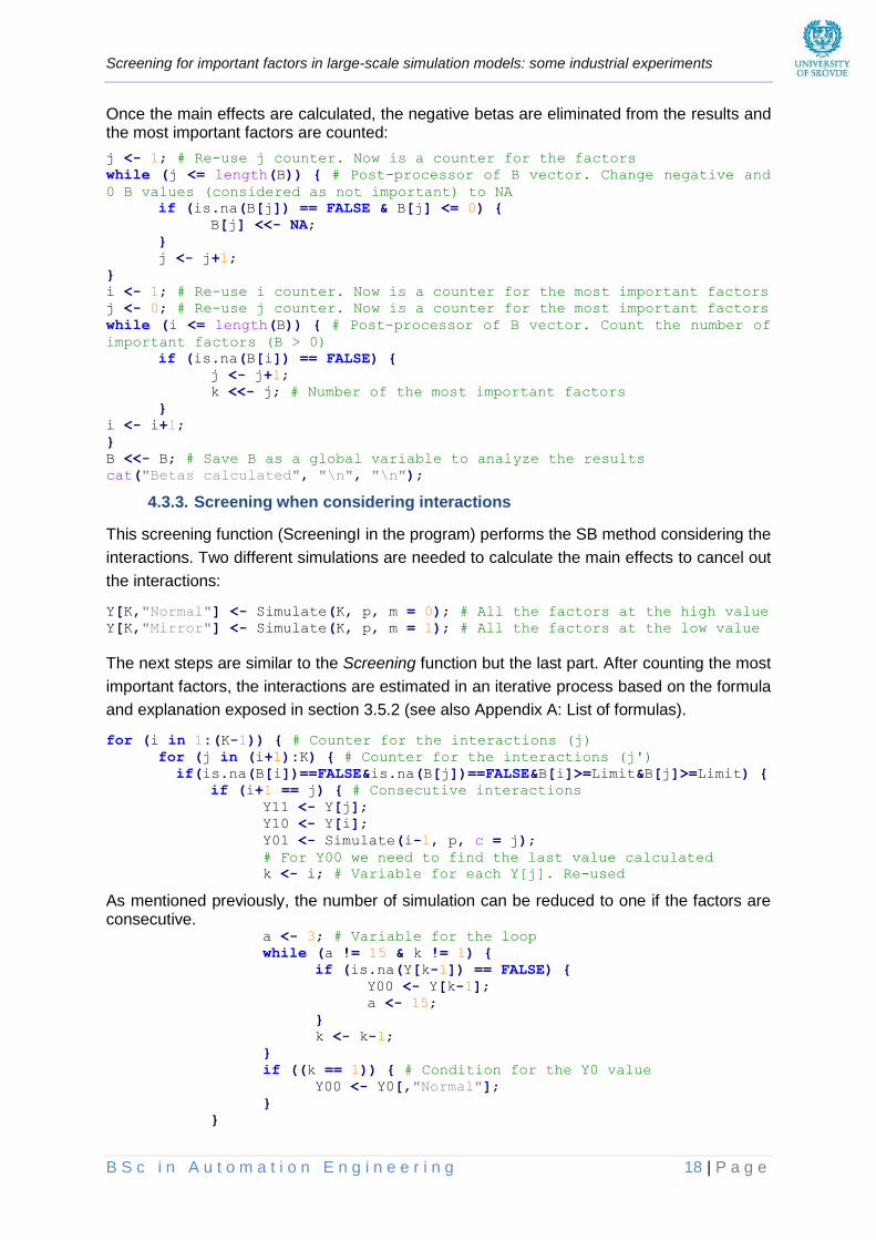
4.3.3. Screening when considering interactions
This screening function (ScreeningI in the program) performs the SB method considering the
interactions. Two different simulations are needed to calculate the main effects to cancel out
the interactions:
Y[K,"Normal"] <- Simulate(K, p, m = 0); # All the factors at the high value
Y[K,"Mirror"] <- Simulate(K, p, m = 1); # All the factors at the low value
The next steps are similar to the Screening function but the last part. After counting the most
important factors, the interactions are estimated in an iterative process based on the formula
and explanation exposed in section 3.5.2 (see also Appendix A: List of formulas).
for (i in 1:(K-1)) { # Counter for the interactions (j)
for (j in (i+1):K) { # Counter for the interactions (j')
if(is.na(B[i])==FALSE&is.na(B[j])==FALSE&B[i]>=Limit&B[j]>=Limit) {
if (i+1 == j) { # Consecutive interactions
Y11 <- Y[j];
Y10 <- Y[i];
Y01 <- Simulate(i-1, p, c = j);
# For Y00 we need to find the last value calculated
k <- i; # Variable for each Y[j]. Re-used
As mentioned previously, the number of simulation can be reduced to one if the factors are consecutive. a <- 3; # Variable for the loop
while (a != 15 & k != 1) {
if (is.na(Y[k-1]) == FALSE) {
Y00 <- Y[k-1];
a <- 15;
}
k <- k-1;
}
if ((k == 1)) { # Condition for the Y0 value
Y00 <- Y0[,"Normal"];
}
}

Screening for important factors in large-scale simulation models: some industrial experiments
B S c i n A u t o m a t i o n E n g i n e e r i n g 19 | P a g e
If the factors are not consecutive, the interaction are calculated as follows.
else {
Y11 <- Simulate(i, p, c = j);
Y10 <- Y[i];
Y01 <- Simulate(i-1, p, c = j);
# For Y00 we need to find the last value calculated, as follows
k <- i; # Variable for each Y[j]. Re-used
a <- 3; # Variable for the loop
while (a != 15 & k != 1) {
if (is.na(Y[k-1]) == FALSE) {
Y00 <- Y[k-1];
a <- 15;
}
k <- k-1;
}
if ((k == 1)) { # Condition for the Y0 value
Y00 <- Y0[,"Normal"];
}
}
Bi[i,j] <- ((Y11 + Y00) - (Y10 + Y01))/4; # Interaction calculated
4.3.4. Simulate
The simulate function generates the input files, calls the simulator and reads the result from
the output file. These results depend on the output factor studied (p), the number of the factor
to study (n) and whether or not the simulation is for the mirror (m).
if (m == 0) {
InputsSim <- Inputs[,"vhigh"]; # Inputs for the simulation
while (n <= K) { # Re-define the InputsSim vector
InputsSim[n] <- Inputs[n,"vlow"];
n <- n+1;
}
}
...
system("xsim-runner.exe --model=Model.xml --input=InputsSim.txt --
output_txt=OutputsSim.txt", wait = TRUE); # Simulation
...
Outputs <- scan("OutputsSim.txt", quiet = TRUE); # Read the result
Furthermore, this function is used when calculating the interactions by setting a specific factor
to its high value.
if (c != 0) {
InputsSim[c] <- Inputs[c,"vhigh"]; }
4.3.5. Results
The results function generates the output files of the SB, save the R image and send the
results by email. This function also creates the graphs: Pareto graphs, most important factors,
group bifurcations and most important interactions graph when corresponding.
4.4. Summary of the chapter
R has been selected as the programming language to develop the automated program of the
SB due to its flexibility and graphic capabilities. Hence, it should be noted that this automation
is not only about the SB, it also includes the automated generation of the graphics, which are
used especially to show and compare the results with the optimization study.

Screening for important factors in large-scale simulation models: some industrial experiments
B S c i n A u t o m a t i o n E n g i n e e r i n g 20 | P a g e
5. INDUSTRIAL SIMULATION MODELS
Explanation of the models to study and their preparatory experiments
This chapter presents four industrial models and their corresponding preparatory experiments,
steady state analysis and replication analysis, which are described and explained in detail.
5.1. Table Production Simulation model (TPS)
The first industrial model studied originates from the University of Skövde and it is used in
different simulation courses to learn modeling and analysis of production systems. However,
it has enough complexity to be used in more advanced techniques, as applied in the present
project. TPS model (see figure 8) studies a production line of tables and it contains different
variants of the product and several material sources to provide the required components.
Figure 8. TPS model. Source: FACTS Analyzer software (University of Skövde)
In this model 42 different factors have been studied, which can be divided into three different
categories:
Buffer capacities of the machines.
Machine MTTRs (Mean Time To Repair).
Machine availabilities.

Screening for important factors in large-scale simulation models: some industrial experiments
B S c i n A u t o m a t i o n E n g i n e e r i n g 21 | P a g e
5.1.1. Steady state analysis: TPS
An important step before starting to experiment with a simulation model is to perform a steady
state analysis and a replication analysis. In regards with the first one, it is necessary to define
an adequate warm-up time and a simulation horizon for the simulation. Thus, the task is to
determine the point where the model reaches a stable state. To study the evolution of the
systems and their stabilization, the WIP and the TH results of the simulation have to be
analyzed.
As figure 9 shows, the system requires approximately 330 (simulated) hours, around 14 days,
to reach a steady state. Regarding the simulation horizon, it has to be long enough to obtain
stable results; therefore, it was set to 100 days.
Figure 9. Steady state of the TPS model. Source: FACTS Analyzer software (University of Skövde)
5.1.2. Replication analysis: TPS
The objective of this experiment is to calculate the number of replications (Rep) required based
on the desired confidence interval (CI). It consists in an iterative process that estimates the
number of replications needed in relation to the number of replications used and the outputs
of the system. After making the estimation the first time, it is necessary to perform a new
simulation with the new number of replications, selecting the larger number of replications (see
Rep results column in table 1), and repeat the iteration until the process is stabilized.
The results from the replication analysis of the TPS model show that 2 replications are enough
to preserve an absolute precision of 0.02. However, based on the delimitations of the present
project, the number of replications was set to 5.
Output CI Rep used Mean Standard deviation
CI (Standard
error)
Rep precision
Absolute precision
Rep results
TH 0.950 10 48.680 0.121 0.086 0.020 0.974 0.079
LT 0.950 10 9.157.856 23.842 17.056 0.020 183.157 0.087
WIP 0.950 10 220.200 0.005 0.003 0.020 4.404 0.000
TH 0.950 2 48.672 0.015 0.139 0.020 0.973 0.041
LT 0.950 2 9.157.694 1.624 14.591 0.020 183.154 0.013
WIP 0.950 2 220.200 0.004 0.033 0.020 4.404 0.000
Table 1. Replication analysis of the TPS model. Source: own elaboration
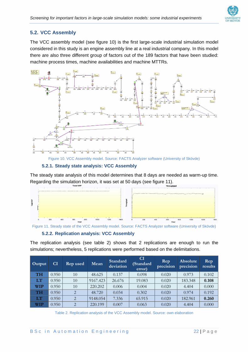
Screening for important factors in large-scale simulation models: some industrial experiments
B S c i n A u t o m a t i o n E n g i n e e r i n g 22 | P a g e
5.2. VCC Assembly
The VCC assembly model (see figure 10) is the first large-scale industrial simulation model
considered in this study is an engine assembly line at a real industrial company. In this model
there are also three different group of factors out of the 189 factors that have been studied:
machine process times, machine availabilities and machine MTTRs.
Figure 10. VCC Assembly model. Source: FACTS Analyzer software (University of Skövde)
5.2.1. Steady state analysis: VCC Assembly
The steady state analysis of this model determines that 8 days are needed as warm-up time.
Regarding the simulation horizon, it was set at 50 days (see figure 11).
Figure 11. Steady state of the VCC Assembly model. Source: FACTS Analyzer software (University of Skövde)
5.2.2. Replication analysis: VCC Assembly
The replication analysis (see table 2) shows that 2 replications are enough to run the
simulations; nevertheless, 5 replications were performed based on the delimitations.
Output CI Rep used Mean Standard deviation
CI (Standard
error)
Rep precision
Absolute precision
Rep results
TH 0.950 10 48.625 0.137 0.098 0.020 0.973 0.102
LT 0.950 10 9167.423 26.676 19.083 0.020 183.348 0.108
WIP 0.950 10 220.202 0.006 0.004 0.020 4.404 0.000
TH 0.950 2 48.720 0.034 0.302 0.020 0.974 0.192
LT 0.950 2 9148.054 7.336 65.915 0.020 182.961 0.260
WIP 0.950 2 220.199 0.007 0.063 0.020 4.404 0.000
Table 2. Replication analysis of the VCC Assembly model. Source: own elaboration

Screening for important factors in large-scale simulation models: some industrial experiments
B S c i n A u t o m a t i o n E n g i n e e r i n g 23 | P a g e
5.3. VCC L-fab
The model for the VCC L-fab machining line is the most complex system studied in this project.
In the VCC L-fab model (see figure 12) 634 factors have been studied, which are divided in
machines machine process times, machine availabilities and machine MTTRs.
Figure 12. VCC L-fab model. Source: FACTS Analyzer software (University of Skövde)
5.3.1. Steady state analysis: VCC L-fab
The warm-up time and the simulation horizon were set to 10 and 50 days, respectively (see
figure 13).
Figure 13. Steady state of the VCC L-fab model. Source: FACTS Analyzer software (University of Skövde)
5.3.2. Replication analysis: VCC L-fab
This model requires between 70 and 87 replications. In spite of this result, 5 replications were
set because the time required is not reachable (see table 3).
Output CI Rep used Mean Standard deviation
CI (Standard
error)
Rep precision
Absolute precision
Rep results
TH 0.950 20 75.807 1.284 0.601 0.020 1.516 3.143
LT 0.950 20 31.122.809 2.493.458 1.166.974 0.020 622.456 70.297
WIP 0.950 20 888.636 50.152 23.472 0.020 17.773 34.883
TH 0.950 50 76.042 1.277 0.363 0.020 1.521 2.848
LT 0.950 50 30.706.140 2.845.021 808.546 0.020 614.123 86.670
WIP 0.950 50 882.848 61.251 17.407 0.020 17.657 48.597
Table 3. Replication analysis of the VCC L-fab model. Source: own elaboration

Screening for important factors in large-scale simulation models: some industrial experiments
B S c i n A u t o m a t i o n E n g i n e e r i n g 24 | P a g e
5.4. NBS
The last large-scale industrial simulation model studied represents a manufacturer production
line. The model (see figure 14) has 189 decision variables in which some of them are buffers.
Particularly one big buffer is located at OP_160, which had been found to be the major
bottleneck in a previous optimization study.
Figure 14. NBS model. Source: FACTS Analyzer software (University of Skövde)
5.4.1. Steady state analysis: NBS
The warm-up time was set to 14 days, whereas the simulation horizon, to 30 days (see fig.15).
Figure 15. Steady state of the NBS model. Source: FACTS Analyzer software (University of Skövde)
5.4.2. Replication analysis: NBS
In this model, 5 replications were set despite the results, which determined 3 (see table 4).
Output CI Rep used Mean Standard deviation
CI (Standard
error)
Rep precision
Absolute precision
Rep results
TH 0.950 2 67.625 0.471 4.235 0.020 1.353 19.613
LT 0.950 2 315.579.225 310.149 2.786.574 0.020 6.311.584 0.390
WIP 0.950 2 44.165.544 22.281 200.184 0.020 883.311 0.103
TH 0.950 3 67.761 0.408 1.015 0.020 1.355 1.682
LT 0.950 3 315.350.612 452.645 1.124.432 0.020 6.307.012 0.095
WIP 0.950 3 44.195.920 54.922 136.433 0.020 883.918 0.071
Table 4. Replication analysis of the NBS model. Source: own elaboration
5.5. Summary of the chapter
In this chapter, the models studied have been described and analyzed. This analysis has been
based on the number and type of factors and also on the preparatory experiments. The
following step in the project is the application of the SB method in each of these models in
order to perform the comparison with SBO.

Screening for important factors in large-scale simulation models: some industrial experiments
B S c i n A u t o m a t i o n E n g i n e e r i n g 25 | P a g e
6. RESULTS
Sequential Bifurcation results and comparison with the optimization study
In this chapter, all the results from the application of the SB and their comparison with the
optimization study are shown. The TPS model has been used for the explanation of the
method whereas the other three, large-scale simulation models, for the comparison between
Sequential Bifurcation and simulation-based optimization.
6.1. TPS
Once the R-program of the SB was finished, it was tested with the TPS model. The results
were satisfactory in terms of application of the method although some discussions related to
the influence of the buffers in the SB and the factors’ ranking emerged with its application.
Firstly, the model was studied without considering the interactions: the method found 12
important factors out of the 42 studied (see figure 16), performing only 20 simulations.
Furthermore, the predominance of the buffer capacities is remarkable; the first seven most
important factors are this kind of factor, among which the most important one is
OP90_Capacity.
Figure 16. Most important factors of the TPS model without considering interactions. Source: own elaboration
On the other hand, when considering interactions the method found 20 most important factors
performing 64 simulations, varying the ranking somewhat (see figure 17).
Figure 17. Most important factors of the TPS model when considering interactions. Source: own elaboration

Screening for important factors in large-scale simulation models: some industrial experiments
B S c i n A u t o m a t i o n E n g i n e e r i n g 26 | P a g e
After finding the important factors, the correctness of the results are tested by making a Pareto
graph. This chart studies the evolution of the TH in relation to the number of changes in the
system, including the standard error.
The results from the Pareto graphs of the TPS model (see figure 18) show that the SB
considering interactions are clearly more accurate than without considering interactions.
Furthermore, one important aspect in this graphic is that the factor Buffer2_Capacity increases
the TH more than the previous factors. It can happen because of the method on its own or for
the necessity to have the previous changes to obtain that increase.
Figure 18. Pareto graphs of the TPS model. Source: own elaboration
Regarding the interactions between two factors (see figure 19), they have been calculated as
explained in section 3.5.1. The most important interaction is between the factors
Store1_Capacity and OP120_Disturbance_Availability, which has a negative effect. It implies
that when both factors are established at their high level, the improvement in the output is not
the sum of their effect.
Moreover, attention should additionally be drawn to the bifurcation procedure that follows for
the SB method. This graph is generated after each experiment and represents the order in
which the factors have been studied, the effects and the value of the importance of the groups
and the most important factors. More precisely, and focusing on the group bifurcations graph
of the TPS model (see figure 20), it is possible to observe that among all the most important
factors, the factor 8, OP90_Capaticy, is one of the factors that have a higher effect on the
output, which agrees with the ranking obtained. However, factor 11, Store1_Capacity, is the
most important factor as studied before; consequently, it should have to be in a higher level
than factor 8. This is not shown in the graph and it happens because group 5-8 has a higher
effect than group 9-11.
It should also be noted that the group bifurcations graphs of the others three models have not
been included in the report because of the high number of factors to study.

Screening for important factors in large-scale simulation models: some industrial experiments
B S c i n A u t o m a t i o n E n g i n e e r i n g 27 | P a g e
Figure 19. Most important interactions of the TPS model. Source: own elaboration

Screening for important factors in large-scale simulation models: some industrial experiments
B S c i n A u t o m a t i o n E n g i n e e r i n g 28 | P a g e
Figure 20. Group bifurcations of the TPS model. Source: own elaboration
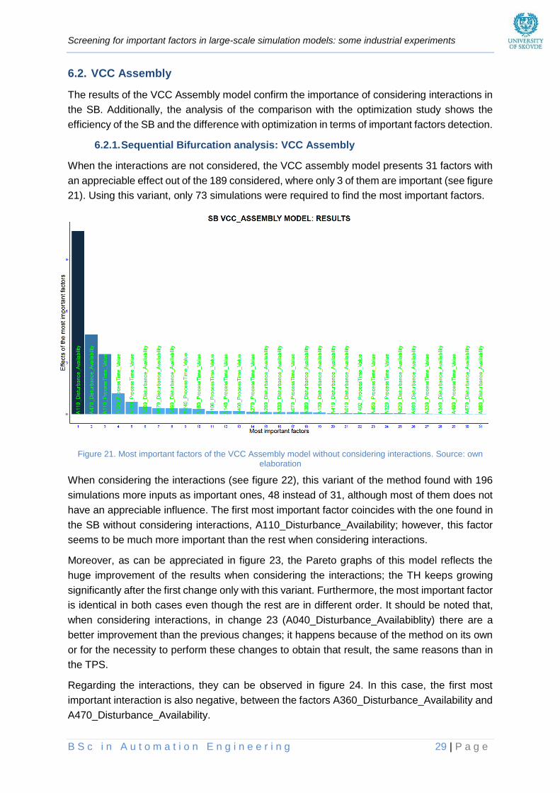
Screening for important factors in large-scale simulation models: some industrial experiments
B S c i n A u t o m a t i o n E n g i n e e r i n g 29 | P a g e
6.2. VCC Assembly
The results of the VCC Assembly model confirm the importance of considering interactions in
the SB. Additionally, the analysis of the comparison with the optimization study shows the
efficiency of the SB and the difference with optimization in terms of important factors detection.
6.2.1. Sequential Bifurcation analysis: VCC Assembly
When the interactions are not considered, the VCC assembly model presents 31 factors with
an appreciable effect out of the 189 considered, where only 3 of them are important (see figure
21). Using this variant, only 73 simulations were required to find the most important factors.
Figure 21. Most important factors of the VCC Assembly model without considering interactions. Source: own elaboration
When considering the interactions (see figure 22), this variant of the method found with 196
simulations more inputs as important ones, 48 instead of 31, although most of them does not
have an appreciable influence. The first most important factor coincides with the one found in
the SB without considering interactions, A110_Disturbance_Availability; however, this factor
seems to be much more important than the rest when considering interactions.
Moreover, as can be appreciated in figure 23, the Pareto graphs of this model reflects the
huge improvement of the results when considering the interactions; the TH keeps growing
significantly after the first change only with this variant. Furthermore, the most important factor
is identical in both cases even though the rest are in different order. It should be noted that,
when considering interactions, in change 23 (A040_Disturbance_Availabiblity) there are a
better improvement than the previous changes; it happens because of the method on its own
or for the necessity to perform these changes to obtain that result, the same reasons than in
the TPS.
Regarding the interactions, they can be observed in figure 24. In this case, the first most
important interaction is also negative, between the factors A360_Disturbance_Availability and
A470_Disturbance_Availability.

Screening for important factors in large-scale simulation models: some industrial experiments
B S c i n A u t o m a t i o n E n g i n e e r i n g 30 | P a g e
Figure 22. Most important factors of the VCC Assembly model when considering interactions. Source: own elaboration

Screening for important factors in large-scale simulation models: some industrial experiments
B S c i n A u t o m a t i o n E n g i n e e r i n g 31 | P a g e
Figure 23. Pareto graphs of the VCC Assembly model. Source: own elaboration

Screening for important factors in large-scale simulation models: some industrial experiments
B S c i n A u t o m a t i o n E n g i n e e r i n g 32 | P a g e
Figure 24. Most important interactions of the VCC Assembly model. Source: own elaboration

Screening for important factors in large-scale simulation models: some industrial experiments
B S c i n A u t o m a t i o n E n g i n e e r i n g 33 | P a g e
6.2.2. Comparison with the optimization study: VCC Assembly
VCC Assembly was the first large-scale model with which the comparison of the SB and
optimization started to be analyzed. A Pareto graph of the optimization ranking was performed
to do the comparison, which was mixed with the corresponding Pareto graph of the SB.
Based on these graphs, as represented in figure 25, it can be observed that the output of the
system is statistically the same until the change number eight due to the overlap of the
standard error, except for the third change. After the ninth change, the outputs from the
optimization are better than the ones from the SB; this difference is caused because
optimization improves the factor A040_Disturbance_Availability in that point, whereas the SB
does not select this factor as important until the 23th position (see figure 22). As stated
previously, this change improves the system more than the changes before, which is an
interesting aspect to be analyzed. This fact is commented in the discussions part of the present
project.
Figure 25. Comparison of SB and optimization in the VCC Assembly model: Pareto graphs. Source: own elaboration
The VCC Assembly model experiments emphasized that the Sequential Bifurcation method is
almost as accurate as the optimization even though a reduction of accuracy is manifested
when performing many changes. Moreover, the SB is clearly more efficient than optimization,
especially in terms of number of simulations, as can be observed in the comparison table
shown in table 5.
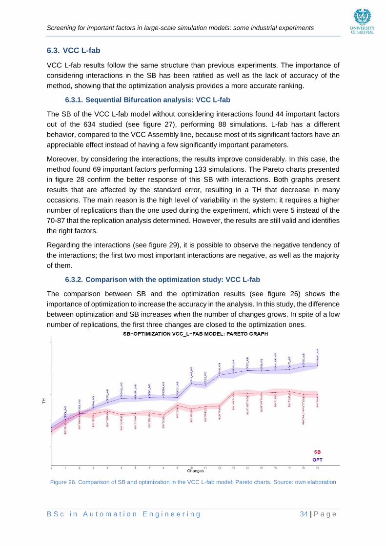
Screening for important factors in large-scale simulation models: some industrial experiments
B S c i n A u t o m a t i o n E n g i n e e r i n g 34 | P a g e
6.3. VCC L-fab
VCC L-fab results follow the same structure than previous experiments. The importance of
considering interactions in the SB has been ratified as well as the lack of accuracy of the
method, showing that the optimization analysis provides a more accurate ranking.
6.3.1. Sequential Bifurcation analysis: VCC L-fab
The SB of the VCC L-fab model without considering interactions found 44 important factors
out of the 634 studied (see figure 27), performing 88 simulations. L-fab has a different
behavior, compared to the VCC Assembly line, because most of its significant factors have an
appreciable effect instead of having a few significantly important parameters.
Moreover, by considering the interactions, the results improve considerably. In this case, the
method found 69 important factors performing 133 simulations. The Pareto charts presented
in figure 28 confirm the better response of this SB with interactions. Both graphs present
results that are affected by the standard error, resulting in a TH that decrease in many
occasions. The main reason is the high level of variability in the system; it requires a higher
number of replications than the one used during the experiment, which were 5 instead of the
70-87 that the replication analysis determined. However, the results are still valid and identifies
the right factors.
Regarding the interactions (see figure 29), it is possible to observe the negative tendency of
the interactions; the first two most important interactions are negative, as well as the majority
of them.
6.3.2. Comparison with the optimization study: VCC L-fab
The comparison between SB and the optimization results (see figure 26) shows the
importance of optimization to increase the accuracy in the analysis. In this study, the difference
between optimization and SB increases when the number of changes grows. In spite of a low
number of replications, the first three changes are closed to the optimization ones.
Figure 26. Comparison of SB and optimization in the VCC L-fab model: Pareto charts. Source: own elaboration

Screening for important factors in large-scale simulation models: some industrial experiments
B S c i n A u t o m a t i o n E n g i n e e r i n g 35 | P a g e
Figure 27. SB results of the VCC L-fab model. Source: own elaboration
SB VCC L-FAB MODEL: RESULTS

Screening for important factors in large-scale simulation models: some industrial experiments
B S c i n A u t o m a t i o n E n g i n e e r i n g 36 | P a g e
Figure 28. Pareto graphs of the VCC L-fab model. Source: own elaboration
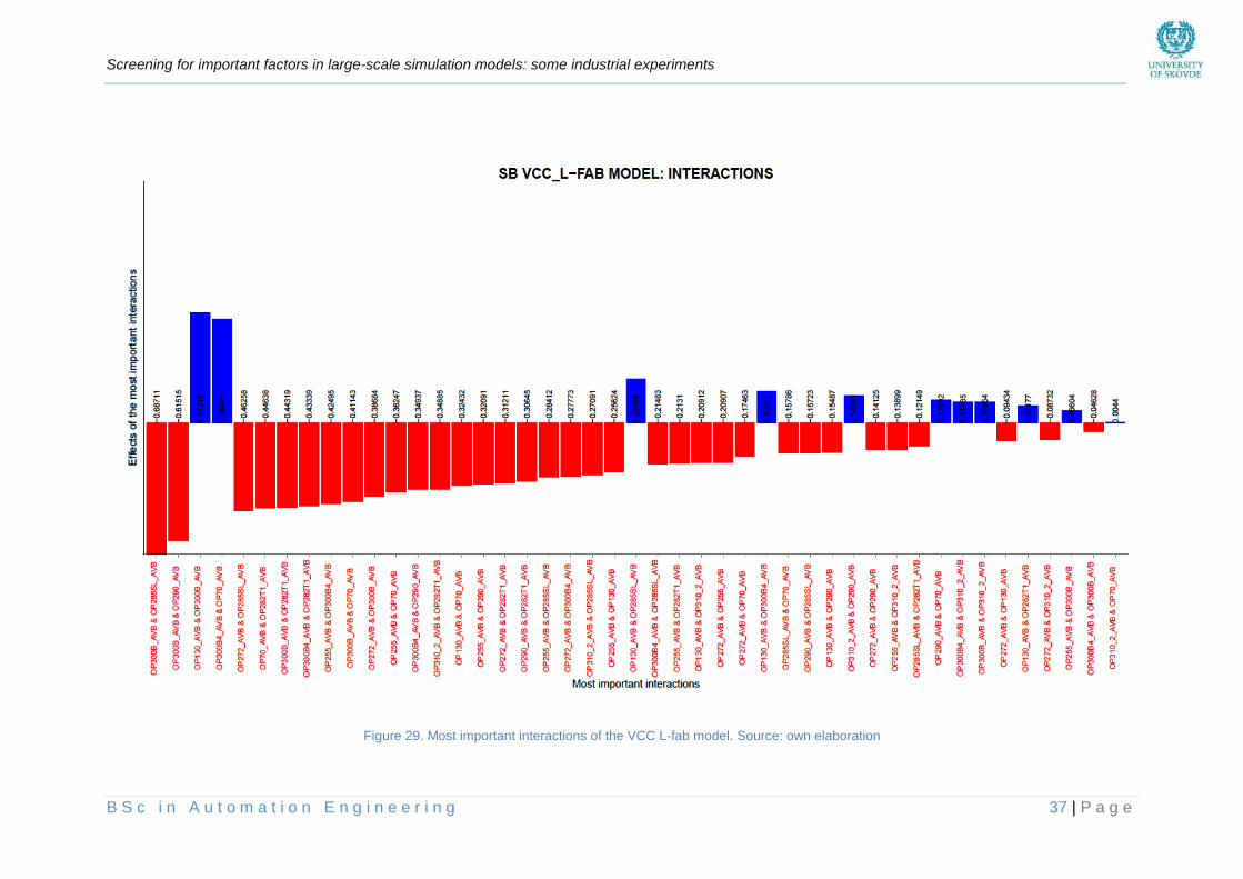
Screening for important factors in large-scale simulation models: some industrial experiments
B S c i n A u t o m a t i o n E n g i n e e r i n g 37 | P a g e
Figure 29. Most important interactions of the VCC L-fab model. Source: own elaboration
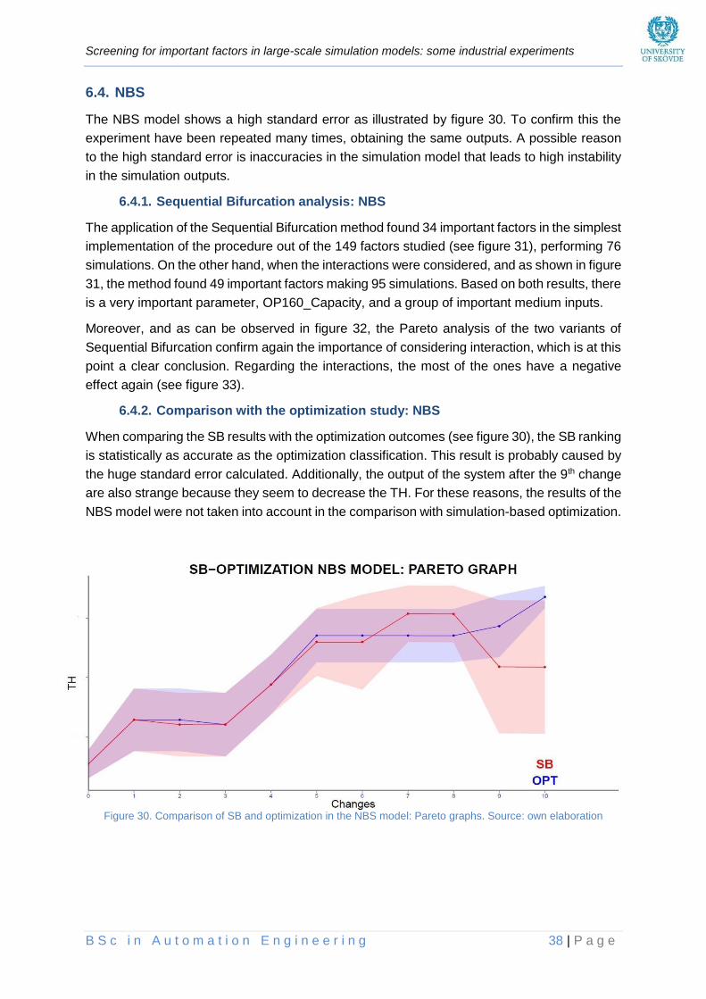
Screening for important factors in large-scale simulation models: some industrial experiments
B S c i n A u t o m a t i o n E n g i n e e r i n g 38 | P a g e
6.4. NBS
The NBS model shows a high standard error as illustrated by figure 30. To confirm this the
experiment have been repeated many times, obtaining the same outputs. A possible reason
to the high standard error is inaccuracies in the simulation model that leads to high instability
in the simulation outputs.
6.4.1. Sequential Bifurcation analysis: NBS
The application of the Sequential Bifurcation method found 34 important factors in the simplest
implementation of the procedure out of the 149 factors studied (see figure 31), performing 76
simulations. On the other hand, when the interactions were considered, and as shown in figure
31, the method found 49 important factors making 95 simulations. Based on both results, there
is a very important parameter, OP160_Capacity, and a group of important medium inputs.
Moreover, and as can be observed in figure 32, the Pareto analysis of the two variants of
Sequential Bifurcation confirm again the importance of considering interaction, which is at this
point a clear conclusion. Regarding the interactions, the most of the ones have a negative
effect again (see figure 33).
6.4.2. Comparison with the optimization study: NBS
When comparing the SB results with the optimization outcomes (see figure 30), the SB ranking
is statistically as accurate as the optimization classification. This result is probably caused by
the huge standard error calculated. Additionally, the output of the system after the 9th change
are also strange because they seem to decrease the TH. For these reasons, the results of the
NBS model were not taken into account in the comparison with simulation-based optimization.
Figure 30. Comparison of SB and optimization in the NBS model: Pareto graphs. Source: own elaboration

Screening for important factors in large-scale simulation models: some industrial experiments
B S c i n A u t o m a t i o n E n g i n e e r i n g 39 | P a g e
Figure 31. SB results of the NBS model. Source: own elaboration
SB VCC NBS MODEL: RESULTS

Screening for important factors in large-scale simulation models: some industrial experiments
B S c i n A u t o m a t i o n E n g i n e e r i n g 40 | P a g e
Figure 32. Pareto graphs of the NBS model. Source: own elaboration

Screening for important factors in large-scale simulation models: some industrial experiments
B S c i n A u t o m a t i o n E n g i n e e r i n g 41 | P a g e
Figure 33. Most important interactions of the NBS model. Source: own elaboration

Screening for important factors in large-scale simulation models: some industrial experiments
B S c i n A u t o m a t i o n E n g i n e e r i n g 42 | P a g e
6.5. Summary of the results
Once the results of the experiments have been collected and analyzed, there are some
aspects that should be emphasized.
First of all, a crucial requirement for considering interactions has been perceived. The
accuracy of the method increases enormously, providing a more precise ranking of the
important factors. This fact was contrasted with all the models studied and especially in the
VCC Assembly model, in which from the first change the results of the SB when considering
interactions were better than the ones without considering them.
Moreover, the efficiency of the method has been proved. Sequential Bifurcation requires a
fraction of the simulations normally needed by an equivalent optimization study. This is
quantified in table 5, which represents the number of simulations required by the simulation-
based optimization study, the SB and the SB when considering interactions, to find the most
important factor of the models studied in the present project.
The TPS and NBS model, as stated previously, were not taken into account to the comparison
with Simulation-based optimization: the first one because it is a student model that has served
to explain and test the SB; the second one, because of its strange and not validated results.
Table 5. Simulations required by SBO, SB and SBi to find the most important factors. Source: own elaboration
Despite its promising results there is a drawback with the SB approach, the simulation-based
optimization solutions are better than the ones delivered by the Sequential Bifurcation
procedure, even though in some cases they offer the same results. More precisely, by
analyzing the SB-OPT graphs generated, it is possible to observe that in most of them until
the third change the results from SB and SBO are statistically the same. However, from this
change the results of optimization are much better. The version compared with SBO was the
SB when considering interactions because it is totally more accurate that the SB without
considering them. Besides, the Pareto charts were calculated with a standard error (shadow
part in the graphs) and also with a confidence error, although this have not been shown in the
report.
Finally, an important influence of the buffers in the SB and some incongruences in the results
have been detected. These aspects as well as the reliability of the method are discussed in
the following chapter.
MODEL SBO SB SBi
TPS - 20 64
VCC Assembly 15000 73 196
VCC L-fab 20000 88 133
NBS 20000 76 95

Screening for important factors in large-scale simulation models: some industrial experiments
B S c i n A u t o m a t i o n E n g i n e e r i n g 43 | P a g e
7. DISCUSSIONS
Effect of the buffers, reliability of the method and congruence of the results
The results obtained during this project imply the discussion of some aspects related to the
Sequential Bifurcation procedure.
One of the most important aspects to take into account when applying SB is the type of factors
to study. The results of the experiments showed that the buffers have an important effect on
the ranking of most important factors. In the models studied, the buffers usually become the
most important factors with a big difference compared to others parameters. Figure 34 shows
this aspect; the most important factors both in the SB when considering and non-considering
interactions are buffers. This situation has to be taken into consideration because it could hide
the importance of the other factors. Two possible approaches can therefore be considered to
mitigate this predominance: 1) Do not include buffers in the inputs of the method or 2) Reduce
the range in which the buffer sizes can vary.
Figure 34. Buffers’ influence in the SB: TPS model example. Source: own elaboration
Another aspect to contemplate is the number of replications, which affects especially the
accuracy of the results. Therefore, finding a good level between exactness and computer time
efficiency should be prioritized. In this project, the VCC L-fab model had to be studied with
fewer replications than the required ones because of the computing time that they required.
Despite that, the results were valid in terms of SB-optimization comparison.
Regarding the reliability of the method, there are some minor inconsistencies that have to be
considered. For instance, in the TPS model, β40−42 is lower than β42 (see figure 20) which is
an incongruence with the SB assumptions and affects to the accuracy of the method. This
happens because the metamodel used by the SB procedure is a simplification of the real
response of the systems. All these simplifications notwithstanding, the results are undeniably
consistent and closed to the optimization results.
Moreover, another aspect to consider is the values in which the factors can vary. SBO
analyzes the factors using more than two levels. This aspect improves the accuracy of the
study, especially when the inputs do not affect linearly to the output of the system. However,
this feature is not implemented in Sequential Bifurcation. The SB studies the factors by giving
them two levels, low and high, as explained in chapter 3. Unfortunately, the implementation of
more factor levels would probably not be possible due to the original metamodel.

Screening for important factors in large-scale simulation models: some industrial experiments
B S c i n A u t o m a t i o n E n g i n e e r i n g 44 | P a g e
Regarding the congruence of the results, the Pareto graphs shows that in some cases, a
specific change improves the TH more than the previous changes, which could be considered
strange. In its majority, the effect of this change depends on the previous improvements, i.e.
without these previous improvements, the effect observed would be shorter. Nevertheless, in
other cases it could be caused by a wrong ranking of the factors.
A specific study was performed to check this incongruence. Figure 35 shows the original
results from the TPS model and the outcomes after modifying the ranking by applying change
number 7 in the fifth position, which was decided after observing an uncommon improvement
when Buffer2_Capacity change was implemented. As can be observed, the results from the
new ranking are better than the old ones in terms of improving the TH. Therefore, it is possible
to conclude certain lack of accuracy in the method.
Figure 35. Incongruence of the results: An experiment with the TPS model. Source: own elaboration
Finally, the main impression of the present study is that these two techniques should be
combined. This mixture could be performed by running Sequential Bifurcation first, considering
all the factors, follow by optimization, using the ranking provided by the SB as inputs. Such a
combination of SB and SBO techniques is already under implementation at the University of
Skövde, obtaining important improvements in terms of efficiency, as figure 36 shows. In this
picture, it is possible to observe the improvement when implementing SB with optimization,
compared with the classical startup of the optimization.
Figure 36. Combination of SB and optimization: initial results. Source: Sunith Bandaru (University of Skövde)

Screening for important factors in large-scale simulation models: some industrial experiments
B S c i n A u t o m a t i o n E n g i n e e r i n g 45 | P a g e
8. CONCLUSIONS
Main conclusions of the present project and future research proposed
The present project discusses the application of screening techniques in large-scale
simulation models, and more precisely, Sequential Bifurcation, with the objective of
determining whether this kind of procedures could be a substitute for or a complement to
simulation-based optimization. After analyzing the results, and based on the objectives and
the procedure followed during the project, there are some important conclusions to mention.
8.1. Main conclusions
All the objectives proposed have been achieved. Their accomplishment is described next:
1. Understand and describe the Sequential Bifurcation method.
The present project has described the SB. The main variants of the original procedure
have also been summarized and analyzed. Besides, the knowledge acquired during this
stage has been used for the correct implementation of the SB R-program.
2. Develop a computer program for the application of the Sequential Bifurcation method.
The development of the computer program for the application of the Sequential Bifurcation
method has been the most difficult and time consumed task during the project. The
program has permitted to run the method in most complex models, which could be
impossible to study without this automation. Furthermore, other sub-objectives have been
also achieved with regards to the development of the program, such us the structuring of
the code of the method into different functions, the automated plotting of the graphs and
the developing of the code to create a Pareto chart in order to compare the results.
3. Analyze the reliability of the Sequential Bifurcation method.
The analysis has been made by analyzing the Pareto charts, comparing the ascending
curve of the TH both in the SB and SBO. The comparison showed the lack of accuracy of
the SB, especially when there are many storage buffers in the decision variables list,
providing worse improvements than SBO even though they were close in some of the
models. Therefore, the necessity of using simulation-based optimization is confirmed.
Moreover, by analyzing the results in detail, there are some conclusions to draw:
First of all, the crucial effect of considering the interactions has been tested. By considering
the interactions, the results are significantly more accurate. Additionally, this project has
exposed the possibility of affecting the society by improving the optimization process and the
efficiency of the systems under study. Indirectly, this project contributes to improving
sustainability if the models consider environmental factors.
Furthermore, the efficiency of Sequential Bifurcation has been confirmed. The results show
that the application of the SB can considerably reduce the simulation time because of the
number of simulations needed, which are totally fewer than the used for SBO.
As a final conclusion, the screening techniques cannot be a complete alternative to simulation-
based optimization. However, the combination of these two methods could set an interesting
alternative to investigate, which is strongly suggested by the authors of this project.

Screening for important factors in large-scale simulation models: some industrial experiments
B S c i n A u t o m a t i o n E n g i n e e r i n g 46 | P a g e
8.2. Future research proposed
The main research to propose after finishing this project is the combination of Sequential
Bifurcation and Simulation-Based Optimization. As stated before, this mixture could be
performed by running Sequential Bifurcation first, considering all the factors, follow by
optimization, using the ranking provided by the SB as inputs. In this sense, some initial results
of this combination have been shown in the discussions part of the present report.
Additionally, some more advanced research could be performed in this context. After the
hypothetical startup of the optimization based on the SB results, the iterative simulations
required by the frequency analysis could be exploited as feedback for the SB procedure to
reassess the factors considered as unimportant. These new estimations could be used to
redirect the optimization.
Another important aspect regarding the potential implementation of this method is the
possibility of making parallel simulations to reduce the time required for the method. When SB
divides a group into two different subgroups, these subgroups could be studied independently
in different computers. However, both subgroups will not probably require the same amount
of simulations hence the workload in each computer will not be similar, which is a drawback.
Therefore, implementing parallel simulations in the method is proposed to be studied.
As stated before, the screening techniques cannot be a complete alternative to simulation-
based optimization. However, the combination of these two methods could yield a promising
roadmap for future research, which is highly recommended by the authors of this project.

Screening for important factors in large-scale simulation models: some industrial experiments
B S c i n A u t o m a t i o n E n g i n e e r i n g 47 | P a g e
REFERENCES
Bettonvil, B. & Kleijnen, J. P., 1996. Searching for important factors in simulation models with
many factors: Sequential bifurcation. European Journal of Operational Research, Volume 96,
pp. 180-194.
Carson, Y. & Anu, M., 1997. Simulation optimization: Methods and applications. New York,
Proceedings of the 1997 Winter Simulation Conference.
Cheng, R. C. H., 1997. Searching for important factors: sequential bifurcation under
uncertainty. Atlanta, Proceedings of the 1997 Winter Simulation Conference, pp. 275-280.
Dorfman, R., 1943. The detection of defective members of large populations. Annals of
Mathematical Statistics, Volume 14, pp. 436-440.
Dupuy, D., Corre, B., M., C.-B. & Sergent, M., 2014. Comparison of different screening
methods. Case Studies In Business, Industry And Government Statistics, 5(2), pp. 115-125.
Frazier, P., Jedynak, B. & Chen, L., 2012. Sequential screening: A Bayesian dynamic
programming analysis of optimal group-splitting. Berlin, Proceedings of the 2012 Winter
Simulation Conference.
Hietala-Koivu, R., 1999. Agricultural landscape change: a case study in Yläne, southwest
Finland. Landscape and Urban Planning, 46(1-3), pp. 103-108.
Hoad, K., Robinson, S. & Davies, R., 2007. Automating DES output analysis: how many
replications to run. New York, Proceedings of the 2007 Winter Simulation Conference.
Karnon, J. et al., 2012. Modeling Using Discrete Event Simulation: A Report of the ISPOR-
SMDM Modeling Good Research Practices Task Force-4. Medical Decision Making, 32(5),
pp. 701-711.
Kleijnen, J., Bettonvil, B. & Persson, F., 2006. Screening for the important factors in large
discrete-event simulation models: sequential bifurcation and its applications. In: A. Dean & S.
Lewis, eds. Screening: Methods for Experimentation in Industry, Drug Discovery, and
Genetics. New York: Springer New York, pp. 287-307.
Kleijnen, J. P., 1998. Experimental design for sensitivity analysis, optimization, and validation
of simulation models. In: J. Banks, ed. Handbook of simulation: Principle, methodology,
advances, applications and practice. New York: John Wiley & Sons, Inc, pp. 173-221.
Law, A. M., 2003. How to conduct a successful simulation study. Tucson, Proceedings of the
2003 Winter Simulation Conference.
Law, A. M., 2009. How to build valid and credible simulation models. Austin, Proceedings of
the 2009 Winter Simulation Conference, pp. 24-33.
Law, A. M., 2014. A tutorial on design of experiments for simulation modeling. Savanah, GA,
Proceedings of the 2014 Winter Simulation Conference, pp. 66-80.
Mahajan, P. S. & Ingalls, R. G., 2004. Evaluation of methods used to detect warm-up period
in steady state simulation. Oklahoma, Proceedings of the 2004 Winter Simulation Conference.
Screening for important factors in large-scale simulation models: some industrial experiments
B S c i n A u t o m a t i o n E n g i n e e r i n g 48 | P a g e
Morris, M. D., 1987. Two-stage factor screening procedures using multiple grouping
assignments. Communications in Statistics - Theory and Methods, 16(10), pp. 3051-3067.
Ng, A., Pehrsson, L. & Bernedixen, J., 2014. What does multi-objective optimization have to
do with bottleneck improvement of production systems?. Skövde, Proceedings of The 6th
International Swedish Production Symposium 2014.
Ng, A., Svensson, J. & Urenda, M., 2008. Multi-Objective Simulation Optimisation for
Production Systems Design using FACTS Analyser. Skövde, Swedish Production Symposium
2008.
Riley, L. A., 2013. Discrete-event simulation optimization: a review of past approaches and
propositions for future direction. Vista, Society for Modeling & Simulation International.
Sanchez, S., Wan, H. & Lucas, T., 2005. A two-phase screening procedure for simulation
experiments. New York, Proceedings of the 2005 Winter Simulation Conference, pp. 223-230.
Satterthwaite, F., 1959. Random Balance Experimentation. Technometrics, 1(2), pp. 111-137.
Shannon, R. E., 1976. Simulation modeling and methodology. Alabama, Winter Simulation
Conference 1976, pp. 33-38.
Shi, W., Shang, J., Liu, Z. & Zuo, X., 2014. Optimal design of the auto parts supply chain for
JIT operations: Sequential bifurcation factor screening and multi-response surface
methodology. European Journal of Operational Research, 236(2), pp. 664-676.
Wan, H., Ankenman, B. & Nelson, B., 2003. Controlled sequential bifurcation: a new factor-
screening method for discrete-event simulation. Evanston, Proceedings of the 2003 Winter
Simulation Conference, pp. 565 - 573.
Watson, G., 1961. A study of the group screening method. Technometrics, Volume 3, pp. 371-
388.
Yaesoubi, R. & Roberts, S., 2007. Important factors in screening for Colorectal Cancer.
Washington, DC, Proceedings of the 2007 Winter Simulation Conference, pp. 1475 - 1482.

Screening for important factors in large-scale simulation models: some industrial experiments
B S c i n A u t o m a t i o n E n g i n e e r i n g 49 | P a g e
APPENDIX
Appendix A: List of formulas
y = β0 + ∑ βjxj
K
j=1
+ ε Equation 1: Output of the system. First order polynomial
y = β0 + ∑ βjxj
K
j=1
+ ∑ ∑ βj′,jxj′xj
K
j′=j+1
K−1
j=1
Equation 2: First order polynomial augmented with two-factor interactions
βj′−j =y(j) − y(j′−1)
2
Equation 3: Effect of a group when not considering interactions
βj =y(j) − y(j−1)
2
Equation 4: Main effect of a factor when not considering interactions
βj′−j =(y(j) − y−(j)) − (y(j′−1) − y−(j′−1))
4
Equation 5: Effect of a group when considering two-factor interactions
βj =(y(j) − y−(j)) − (y(j−1) − y−(j−1))
4
Equation 6: Main effect of a factor when considering two-factor interactions
βa,b =(y++ + y−−) − (y+− + y−+)
4
Equation 7: Effect of an interaction between two factors
Number of interactions (n) =n2 − n
2 Equation 8: Number of interactions
Screening for important factors in large-scale simulation models: some industrial experiments
B S c i n A u t o m a t i o n E n g i n e e r i n g 50 | P a g e
Appendix B: SB R-program
# PROGRAMMERS: Rafael Adrian Garcia Martin (Ragm93) & Jose Manuel
Gaspar Sanchez (Jmsg) / 12-06-2015
SB <- function() { # This is the main function of the method
# MAIN FUNCTIONS
Packages(); # In this function, all the complements needed in
the simulation are loaded
Reset(); # In this function, all the global variables are
reset
Decisions(); # In this function, the configuration of the
study is set
Start(); # This is the function that starts the corresponding
method
Pareto(); # This function is in charge of calculating the
Pareto graph, necessary to compare the SB results with the
optimization study
Results(); # This function shows the results of the SB method
}
# FUNCTIONS DEFINITION
Packages <- function() { # In this function, all the
complements needed in the simulation are loaded
cat("\n");
cat("LOADING THE REQUIRED PACKAGES", "\n", "\n");
install.packages("ggplot2", repos =
"http://cran.rstudio.com"); # Required for plotting
install.packages("Rcpp", repos =
"http://cran.rstudio.com"); # Required for plotting
install.packages("colorspace", repos =
"http://cran.rstudio.com"); # Required for plotting
install.packages("sendmailR", repos =
"http://cran.rstudio.com"); # Required to send emails from R
install.packages("XLConnect", repos =
"http://cran.rstudio.com"); # Required to extract info from Excel
files
install.packages("XML", repos =
"http://cran.rstudio.com"); # Required to load the info from XML
files
require(ggplot2);
require(sendmailR);
require(XLConnect);
require(XML);
cat("\n");
cat("PACKAGES LOADED", "\n", "\n");
}
Reset <- function() { # In this function, all the global
variables are reset
MN <<- 0; # Model name
S <<- 0; # Type of SB

Screening for important factors in large-scale simulation models: some industrial experiments
B S c i n A u t o m a t i o n E n g i n e e r i n g 51 | P a g e
parameter <<- 0; # Type of parameter to study (string)
Mails <<- 0; # Used to decide sending mails or not
n <<- 0; # Number of replications to do
alpha <<- 0; # alpha value for the confidence interval
selected
p <<- 0; # Type of parameter to study (num)
T0 <<- 0; # Simulation start time
Inputs <<- 0; # Excel data
K <<- 0; # Number of variables of the system
s <<- 0; # Number of simulations
Y <<- 0; # SB Y objective function
M <<- 0; # "Work to do" matrix
U <<- 0; # Upper limits matrix
Y0 <<- 0; # SB Y[0]
Bi <<- 0; # Interactions matrix
Biplot <<- 0; # Interactions matrix for the plotting
B <<- 0; # SB main effects vector
B0 <<- 0; # SB B0
k <<- 0; # Number of most important factors
OV <<- 0; # Other values: Y0 and B0
TF <<- 0; # Finish time of the simulation
TF2 <<- 0; # Finish time of the simulation (replacing :
to .)
Plot_data_Pareto <<- 0; # Data used for the graphics.
Pareto chart
Graph_Pareto <<- 0; # Graph for the Pareto chart
(Standard error)
Graph_Pareto_CI <<- 0; # Graph for the Pareto chart
(confidence interval)
Tt <<- 0; # Average time per simulation
Plot_data_MIF <<- 0; # Data used for the graphics. Betas
Plot_data_Interactions <<- 0; # Data used for the
graphics. Interactions
Plot_data_Bifurcations <<- 0; # Data used for the
graphics. Group bifurcations
Graph_Factors <<- 0; # Graphics. Betas
Graph_Interactions <<- 0; # Graphics. Interactions
Graph_Bifurcations <<- 0; # Graphics. Group bifurcations
}
Decisions <- function() { # In this function, the
configuration of the study is set
# PART 1: Working directory
cat("\n");
cat("CONFIGURATIONS OF THE METHOD", "\n", "\n");
a <- 3;
while (a != 15) {
cat("Select your working directory:", "\n");
cat("1 --> FACTS folder", "\n");
cat("2 --> Other folder", "\n", "\n");
answer <- readline();
if (answer == "1") {
setwd("C:\\FACTS");

Screening for important factors in large-scale simulation models: some industrial experiments
B S c i n A u t o m a t i o n E n g i n e e r i n g 52 | P a g e
cat("\n", "C:\\FACTS set as working
directory", "\n", "\n", sep = "");
a <- 15;
}
else if (answer == "2") {
cat("\n", "Write the name of your folder: ",
sep = "");
WD <- readline();
if (file.exists(paste("C:\\", WD, sep = ""))){
setwd(paste("C:\\", WD, sep = ""));
cat("\n", "C:\\", WD, " already exists.
Set as working directory", "\n", "\n", sep = "");
}
else {
dir.create(paste("C:\\", WD, sep = ""));
setwd(paste("C:\\", WD, sep = ""));
cat("\n", "C:\\", WD, " set as working
directory", "\n", "\n", sep = "");
}
a <- 15;
}
else {
cat("\n", "Error. Try again", "\n", "\n", sep
= "");
}
}
# PART 2: Model name
cat("Write the name of your model: ", sep = "");
MN <<- readline();
cat("\n");
# PART 3: Copying files
a <- 3;
while (a != 15) {
cat("Copy the files (Model.xml / Inputs.xlsx /
xsim-runner.exe) into the folder", "\n");
cat("Are the files already copied?", "\n");
cat("1 --> YES", "\n");
cat("2 --> NO", "\n", "\n");
answer <- readline();
cat("\n");
if (answer == "1") {
a <- 15;
}
else if (answer == "2") {
cat("OK. Try again", "\n", "\n", sep = "");
}
else {
cat("Error. Try again", "\n", "\n", sep = "");
}
}

Screening for important factors in large-scale simulation models: some industrial experiments
B S c i n A u t o m a t i o n E n g i n e e r i n g 53 | P a g e
# PART 4: Screening method
a <- 3;
while (a != 15) {
cat("Select the screening method:", "\n");
cat("1 --> Sequential Bifurcation not considering
interactions", "\n");
cat("2 --> Sequential Bifurcation considering
interactions", "\n", "\n");
answer <- readline();
if (answer == "1") {
S <<- 1;
cat("\n", "Sequential Bifurcation not
considering interactions selected", "\n", "\n", sep = "");
a <- 15;
}
else if (answer == "2") {
S <<- 2;
cat("\n", "Sequential Bifurcation considering
interactions selected", "\n", "\n", sep = "");
a <- 15;
}
else {
cat("\n", "Error. Try again", "\n", "\n", sep
= "");
}
}
# PART 5: Parameter to study
a <- 3;
while (a != 15) {
cat("Select the parameter to study:", "\n");
cat("1 --> TH", "\n");
cat("2 --> WIP", "\n");
cat("3 --> Lead time", "\n", "\n");
parameter <<- readline();
if (parameter == "1") {
p <<- 1;
cat("\n", "TH selected", "\n", "\n", sep =
"");
parameter <<- "TH";
a <- 15;
}
else if (parameter == "2") {
p <<- 2;
cat("\n", "WIP selected", "\n", "\n", sep =
"");
parameter <<- "WIP";
a <- 15;
}
else if (parameter == "3") {
p <<- 3;
cat("\n", "Lead time selected", "\n", "\n",
sep = "");
Screening for important factors in large-scale simulation models: some industrial experiments
B S c i n A u t o m a t i o n E n g i n e e r i n g 54 | P a g e
parameter <<- "Lead Time";
a <- 15;
}
else {
cat("\n", "Error. Try again", "\n", sep = "");
cat("\n");
}
}
# PART 6: Pareto information
a <- 3;
while (a != 15) {
cat("Write the number of replications to do: ", sep
= "");
n <<- readline(); # Number of replications done in
the simulation
n <<- as.numeric(n);
cat("\n", "Write the confidence interval you
want(%): ", sep = "");
CI <- readline(); # Confidence interval for the
standard error chart
CI <- as.numeric(CI);
alpha <<- 1-CI/100; # Alpha of the confidence
interval selected
cat("\n");
cat("Number of replications to do: ", n, ";
confidence interval selected: ", CI, " %", "\n", sep = "");
cat("Is it correct?", "\n");
cat("1 --> YES", "\n");
cat("2 --> NO", "\n", "\n");
answer <- readline();
if (answer == "1") {
a <- 15;
cat("\n");
}
else if (answer == "2") {
cat("\n", "OK. Check your inputs", "\n", "\n",
sep = "");
}
else {
cat("\n", "Error. Try again", "\n", "\n", sep
= "");
}
}
# PART 7: Mails
a <- 3;
while (a != 15) {
cat("Select if you want to be notified by email:",
"\n");
cat("1 --> Yes, send me mails", "\n");
cat("2 --> No, I do not want mails", "\n", "\n");
answer <- readline();

Screening for important factors in large-scale simulation models: some industrial experiments
B S c i n A u t o m a t i o n E n g i n e e r i n g 55 | P a g e
if (answer == "1") {
Mails <<- 1;
cat("\n", "Email notifications will be
delivered", "\n", "\n", sep = "");
a <- 15;
}
else if (answer == "2") {
Mails <<- 0;
cat("\n", "No mails will be delivered", "\n",
"\n", sep = "");
a <- 15;
}
else {
cat("\n", "Error. Try again", "\n", "\n", sep
= "");
}
}
cat("METHOD CONFIGURATED", "\n", "\n");
}
Start <- function() { # This is the function which starts the
corresponding method
cat("\n");
cat("CHECKING THE CONFIGURATIONS", "\n");
cat("\n");
a <- 3;
while (a != 15) {
if (S == 1) { # SB not considering interactions
if (Mails == 1) { # Decisions check with mails
notifications
cat("SB method of the model ", MN, "
(located in ", getwd(), ")", ", not considering interactions,
sending mails notifications and studying the ", parameter, " is
about to start:", "\n", sep = "");
}
else { # Decisions check without mails
notifications
cat("SB method of the model ", MN, "
(located in ", getwd(), ")", ", not considering interactions, not
sending mails notifications and studying the ", parameter, " is
about to start:", "\n", sep = "");
}
cat("Continue?", "\n");
cat("1 --> YES", "\n");
cat("2 --> NO", "\n", "\n");
answer <- readline();
if (answer == 1) {
cat("\n");
S <<- "SB";
T0 <<- toString(Sys.time());
if (Mails == 1) { # Sending an email
notification
from <- sprintf("<sendmailR@%s>",

Screening for important factors in large-scale simulation models: some industrial experiments
B S c i n A u t o m a t i o n E n g i n e e r i n g 56 | P a g e
Sys.info()[4]);
dest <- "<[email protected]>";
dest2 <-
"<[email protected]>";
subject <- paste("SCREENING SB
METHOD STARTED.", MN, "MODEL");
msg <- paste("SB method not
considering interactions, studying the ", parameter, ", started
at: ", T0, sep = "");
sendmail(from, dest, subject, msg,
control = list(smTPServer = "ASPMX.L.GOOGLE.COM"));
sendmail(from, dest2, subject, msg,
control = list(smTPServer = "ASPMX.L.GOOGLE.COM"));
}
cat("CONFIGURATIONS CHECKED", "\n",
"\n");
Screening();
a <- 15;
}
else if (answer == 2){
cat("\n", "Restarting", "\n", sep = "");
Decisions();
}
else {
cat("\n", "Error. Try again", "\n",
"\n", sep = "");
}
}
else { # SB considering interactions
if (Mails == 1) { # Decisions check with mails
notifications
cat("SB method of the model ", MN, "
(located in ", getwd(), ")", ", considering interactions, sending
mails notifications and studying the ", parameter, " is about to
start:", "\n", sep = "");
}
else { # Decisions check without mails
notifications
cat("SB method of the model ", MN, "
(located in ", getwd(), ")", ", considering interactions, not
sending mails notifications and studying the ", parameter, " is
about to start:", "\n", sep = "");
}
cat("Continue?", "\n");
cat("1 --> YES", "\n");
cat("2 --> NO", "\n", "\n");
answer <- readline();
if (answer == 1) {
cat("\n");
S <<- "SBi";
T0 <<- toString(Sys.time());
if (Mails == 1) { # Sending an email
Screening for important factors in large-scale simulation models: some industrial experiments
B S c i n A u t o m a t i o n E n g i n e e r i n g 57 | P a g e
notification
from <- sprintf("<sendmailR@%s>",
Sys.info()[4]);
dest <- "<[email protected]>";
dest2 <-
"<[email protected]>";
subject <- paste("SCREENING SB
METHOD STARTED.", MN, "MODEL");
msg <- paste("SB method considering
interactions, studying the ", parameter, ", started at: ", T0, sep
= "");
sendmail(from, dest, subject, msg,
control = list(smTPServer = "ASPMX.L.GOOGLE.COM"));
sendmail(from, dest2, subject, msg,
control = list(smTPServer = "ASPMX.L.GOOGLE.COM"));
}
cat("CONFIGURATIONS CHECKED", "\n",
"\n");
ScreeningI();
a <- 15;
}
else if (answer == 2){
cat("\n", "Restarting", "\n", "\n", sep
= "");
Decisions();
}
else {
cat("\n", "Error. Try again", "\n",
"\n", sep = "");
}
}
}
}
Pareto <- function() { # This function is in charge of
calculating the Pareto graph, necessary to compare with the
optimization study
# PART 1: Variables & Simulation information
cat("\n");
cat("PARETO GRAPH CALCULATIONS", "\n");
cat("\n");
if (S == "SBi") {
SBt <- "WHEN CONSIDERING INTERACTIONS"; # SB
variant tittle (capital letters)
}
else {
SBt <- "WITHOUT CONSIDERING INTERACTIONS"; # SB
variant tittle (capital letters)
}
PFactors <- Inputs[order(B, decreasing = TRUE)[1:k],
"Factor"]; # Most important factors ordered by importance
Name <- c(0:(length(Inputs[order(B, decreasing =

Screening for important factors in large-scale simulation models: some industrial experiments
B S c i n A u t o m a t i o n E n g i n e e r i n g 58 | P a g e
TRUE)[1:k], "Name"]))); # Most important factors names ordered by
importance
Name[1:length(Inputs[order(B, decreasing = TRUE)[1:k],
"Name"])+1] <- Inputs[order(B, decreasing = TRUE)[1:k], "Name"]; #
Adding spot in the Name first string
Name[1] <- "";
ResultPareto <- matrix(NA, length(PFactors)+1, 7); #
Matrix for the Pareto simulations' results
colnames(ResultPareto) <- c("Result", "SD", "Lower",
"Upper", "SE", "Upper_SE", "Lower_SE"); # Re-naming the columns of
the matrix
cat("Pareto simulations initialized", "\n", "\n", sep =
"");
# PART 2: Pareto simulations
cat("Pareto simulation: 1/", length(PFactors)+1, "\n",
sep = "");
R <- ParetoPoint(p); # First simulation
ResultPareto[1,"Result"] <- R[1];
ResultPareto[1,"SD"] <- R[2];
ResultPareto[1,"Upper"] <- ResultPareto[1,"Result"] +
ResultPareto[1,"SD"]; # Lower value for the confidence interval
ResultPareto[1,"Lower"] <- ResultPareto[1,"Result"] -
ResultPareto[1,"SD"]; # Higher value for the confidence interval
ResultPareto[1,"SE"] <- qt((1-alpha/2), df = (n-
1))*(ResultPareto[1,"SD"]/sqrt(n)); # Standard error for each
variable
ResultPareto[1,"Upper_SE"] <- ResultPareto[1,"Result"]
+ ResultPareto[1,"SE"]; # Lower value for the standard error
ResultPareto[1,"Lower_SE"] <- ResultPareto[1,"Result"]
- ResultPareto[1,"SE"]; # Higher value for the standard error
for (i in 1:(length(PFactors))) { # Pareto simulations
of the most important factors
cat("Pareto simulation: ", i+1, "/",
length(PFactors)+1, "\n", sep = "");
R <- ParetoPoint(p, PFactors[1:i]);
ResultPareto[i+1,"Result"] <- R[1];
ResultPareto[i+1,"SD"] <- R[2];
ResultPareto[i+1,"Upper"] <-
ResultPareto[i+1,"Result"] + ResultPareto[i+1,"SD"];
ResultPareto[i+1,"Lower"] <-
ResultPareto[i+1,"Result"] - ResultPareto[i+1,"SD"];
ResultPareto[i+1,"SE"] <- qt((1-alpha/2), df = (n-
1))*(ResultPareto[i+1,"SD"]/sqrt(n));
ResultPareto[i+1,"Upper_SE"] <-
ResultPareto[i+1,"Result"] + ResultPareto[i+1,"SE"];
ResultPareto[i+1,"Lower_SE"] <-
ResultPareto[i+1,"Result"] - ResultPareto[i+1,"SE"];
}
cat("Pareto simulations finished", "\n", "\n", sep =
"");
# PART 3: Data frame for the graphics

Screening for important factors in large-scale simulation models: some industrial experiments
B S c i n A u t o m a t i o n E n g i n e e r i n g 59 | P a g e
Changes <- 0:(length(PFactors)); # x axis
y <- ResultPareto[,"Result"]; # y axis
Upper <- ResultPareto[,"Upper"]; # Higher value for the
confidence interval
Lower <- ResultPareto[,"Lower"]; # Lower value for the
confidence interval
SD <- ResultPareto[,"SD"]; # Standard deviation results
SE <- ResultPareto[,"SE"]; # Standard error results
Upper_SE <- ResultPareto[,"Upper_SE"]; # Higher value
for the standard error
Lower_SE <- ResultPareto[,"Lower_SE"]; # Lower value for
the standard error
Plot_data_Pareto <<- data.frame(Name, Changes, y, SD,
Upper, Lower, SE, Upper_SE, Lower_SE); # Data frame with all the
data to plot
# PART 4: Pareto graph. Standard error
Graph_Pareto <<- ggplot(Plot_data_Pareto, aes(x =
Changes, y = y)); # Creating the graph
Graph_Pareto <<- Graph_Pareto + geom_line(stat =
"identity", colour = "blue") + geom_point(colour = "red") +
geom_ribbon(aes(ymax = Upper_SE, ymin = Lower_SE), alpha = 0.15);
# Main layers of the graph
Graph_Pareto <<- Graph_Pareto + ggtitle(paste("SB", MN,
"MODEL: PARETO GRAPH", SBt)) + labs(x = "Changes", y = parameter,
colour = "", fill = "") + scale_x_discrete(limits = Changes, labels
= Changes) +
geom_text(aes(label = Name, angle = -90, y = y-0.005,
hjust = 0), colour = "green", size = 4) +
theme(text = element_text(size = 20), plot.title =
element_text(size = 25, face = "bold"), axis.text.x =
element_text(colour = "blue", size = 11, angle = 0, vjust = 0),
axis.text.y = element_text(colour = "blue", size = 11, angle = 0,
hjust = 0),
axis.line = element_line(colour = "black"),
panel.background = element_blank(), panel.grid.major =
element_blank(), panel.grid.minor = element_blank(),
legend.position = "none"); # Aesthetic layers added to the main
chart
# PART 5: Pareto graph. Confidence interval
Graph_Pareto_CI <<- ggplot(Plot_data_Pareto, aes(x =
Changes, y = y)); # Creating the graph
Graph_Pareto_CI <<- Graph_Pareto_CI + geom_line(stat =
"identity", colour = "blue") + geom_point(colour = "red") +
geom_ribbon(aes(ymax = Upper, ymin = Lower), alpha = 0.15); # Main
layers of the graph
Graph_Pareto_CI <<- Graph_Pareto_CI +
ggtitle(paste("SB", MN, "MODEL: PARETO GRAPH", SBt, "(MaxMin)")) +
labs(x = "Changes", y = parameter, colour = "", fill = "") +
scale_x_discrete(limits = Changes, labels = Changes) +
geom_text(aes(label = Name, angle = -90, y = y-0.005,
hjust = 0), colour = "green", size = 4) +

Screening for important factors in large-scale simulation models: some industrial experiments
B S c i n A u t o m a t i o n E n g i n e e r i n g 60 | P a g e
theme(text = element_text(size = 20), plot.title =
element_text(size = 25, face = "bold"), axis.text.x =
element_text(colour = "blue", size = 11, angle = 0, vjust = 0),
axis.text.y = element_text(colour = "blue", size = 11, angle = 0,
hjust = 0),
axis.line = element_line(colour = "black"),
panel.background = element_blank(), panel.grid.major =
element_blank(), panel.grid.minor = element_blank(),
legend.position = "none"); # Aesthetic layers added to the main
chart
# PART 6: Finishing the function
save.image(file = paste("0. ", MN, "_", S, ".Rdata", sep
= "")); # Save the image to collect the data in case of error
savehistory();
cat("PARETO GRAPH CALCULATED", "\n", "\n", sep = "");
}
Results <- function() { # This function shows the results of
the SB method
cat("\n");
cat("GENERATING THE GRAPHS", "\n", "\n");
# PART 1: Plot: interactions
if (S == "SBi") {
SB <- "when considering interactions"; # SB variant
graph title
SBt <- "WHEN CONSIDERING INTERACTIONS"; # SB
variant tittle (capital letters)
Factor <- c(1:length(Biplot[,"Name"])); # x axis
Int <-
Biplot[1:length(Biplot[,"Interaction"]),"Interaction"]; # y axis
(modified after)
Name <- Biplot[1:length(Biplot[,"Name"]),"Name"];
# Variables name for the graphics
# Re-defining the variables for the chart
Int0 <- Int; # Keeping the original Int value in
this variable
IntM <- matrix(NA, length(Int0), 3); # Matrix for
the interactions chart. Save the original Interactions values
(Int0), Interactions values for the chart (Int) and colour
information (saved after)
colnames(IntM) <- c("Int0", "Int", "Color"); # Re-
naming the columns of the matrix
IntM[,"Int0"] <- as.numeric(Int);
IntM[,"Int"] <- as.numeric(Int);
Color <- matrix("blue", length(Int), 1); #
Temporary matrix for the colour values
colnames(Color) <- c("Color"); # Re-naming the
columns of the matrix
for (i in 1:length(Int0)) { # Change the values
according to the interactions information: negative values (first
step: negative to positive to order the factors) and colour
information

Screening for important factors in large-scale simulation models: some industrial experiments
B S c i n A u t o m a t i o n E n g i n e e r i n g 61 | P a g e
IntM[i,"Int"] <- IntM[i,"Int0"]*1000; #
Change the scale (better for the plot)
if (IntM[i,"Int0"] < 0) {
IntM[i,"Int"] <- IntM[i,"Int"]*(-1);
Color[i,1] <- "red";
}
IntM[i,"Int0"] <- round(IntM[i,"Int0"],
digits = 5); # Round Interactions values to 5 digits
}
IntM[,"Color"] <- Color[,"Color"]; # Add colour
column to IntM matrix
IntM <- IntM[order(as.numeric(IntM[,"Int"]),
decreasing = TRUE),]; # Order IntM by factors' importance
Int0 <- as.numeric(IntM[,"Int0"]); # Original
Interactions values
Int <- as.numeric(IntM[,"Int"]); # Final x axis
(negative values, modified after)
Color <- IntM[,"Color"]; # Colour values (red -->
negative values; blue --> positive)
for (i in 1:length(Int0)) { # Negative values,
second step
if (IntM[i,"Color"] == "red") {
Int[i] <- Int[i]*(-1);
}
}
# Data frame and chart
Plot_data_Interactions <<- data.frame(Factor,
Int0, Int, Color, Name); # Create a data frame with all the data
to plot (interactions)
Graph_Interactions <<-
ggplot(Plot_data_Interactions, aes(x = Factor, y = Int)); #
Creating the graph
Graph_Interactions <<- Graph_Interactions +
geom_bar(stat = "identity", position = "identity", fill = Color);
# Main layer of the graph
Graph_Interactions <<- Graph_Interactions +
ggtitle(paste("SB", MN, "MODEL: INTERACTIONS")) + labs(x = "Most
important interactions", y = "Effects of the most important
interactions") +
scale_x_discrete(limits = Factor, labels = Name) +
scale_y_discrete(breaks = NULL) + geom_text(aes(label = Int0, angle
= 90, y = 0.0015, hjust = 0), colour = "black", size = 4) +
theme(text = element_text(size = 15), plot.title =
element_text(size = 20, face = "bold"), axis.text.x =
element_text(colour = "red", size = 11, angle = 90, vjust = 0),
axis.line = element_line(colour = "black"),
panel.background = element_blank(),
panel.grid.major = element_blank(), panel.grid.minor =
element_blank()); # Aesthetic layers added to the main chart
}
else {
SB <- "without considering interactions"; # SB
variant graph title

Screening for important factors in large-scale simulation models: some industrial experiments
B S c i n A u t o m a t i o n E n g i n e e r i n g 62 | P a g e
SBt <- "WITHOUT CONSIDERING INTERACTIONS"; # SB
variant tittle (capital letters)
}
# PART 2: Plot: main effects
By <- B; # Equals to B variable (changing NA to 0; done
after)
i <- 1; # Re-used variable. Counter for the names of the
variables and the By vector
for (i in 1:K) { # Replace NA for 0 in By vector
if (is.na(By[i]) == TRUE) {
By[i] <- 0;
}
}
Factor <- c(1:k); # x axis
Beta <- By[order(By, decreasing = TRUE)[1:k]]; # y axis
Name <- Inputs[order(By, decreasing = TRUE)[1:k],
"Name"]; # Variables name for the graphics
Plot_data_MIF <<- data.frame(Factor, Beta, Name); #
Create a data frame with all the data to plot
Graph_MIF <<- ggplot(Plot_data_MIF, aes(x = Factor, y =
Beta, fill = -Beta)); # Creating the graph
Graph_MIF <<- Graph_MIF + geom_bar(stat = "identity");
# Main layer of the graph
Graph_MIF <<- Graph_MIF + ggtitle(paste("SB", MN,
"MODEL: RESULTS")) + labs(x = paste("Most important factors", SB),
y = "Effects of the most important factors", colour = "") +
scale_x_discrete(limits = Factor, labels = Factor) +
geom_text(aes(label = Name, angle = 90, y = 0.0005, hjust = 0),
colour = "green", size = 4) +
theme(text = element_text(size = 20), plot.title =
element_text(size = 25, face = "bold"), axis.text.x =
element_text(colour = "blue", size = 11, angle = 0, vjust = 0),
axis.text.y = element_text(colour = "blue", size = 11,
angle = 0, hjust = 0), axis.line = element_line(colour = "black"),
panel.background = element_blank(), panel.grid.major =
element_blank(), panel.grid.minor = element_blank(),
legend.position = "none"); # Aesthetic layers added to the main
chart
# PART 3: Plot: group bifurcations (this graph is
especially programmed for the TPS model)
# Previous calculations needed
f <- 0; # Counter for the M matrix. Number of rows filled
g <- 0; # Counter for the M matrix. Estimated value for
the number of "factors" plotted
while (is.na(M[f+1,"High"]) == FALSE) { # Calculating
the rows and factors plotted
g <- g + (M[f+1,"High"] - M[f+1,"Low"]); # Factors
f <- f+1; # Rows
}
Data <- matrix(NA, (g+k), 2); # Data for the bifurcation
graph
colnames(Data) <- c("Factor", "Height"); # Re-naming the

Screening for important factors in large-scale simulation models: some industrial experiments
B S c i n A u t o m a t i o n E n g i n e e r i n g 63 | P a g e
columns of the matrix
Color <- matrix("#000099", (g+k), 1); # Matrix for the
color of the factors (blue)
colnames(Color) <- c("Color");
BetaM <- matrix(NA, (g+k), 3); # Data for the bifurcation
graph
colnames(BetaM) <- c("x", "y", "Beta");
U2 <- matrix(NA, (g+k), 1); # Data for the upper limits
text boxes
colnames(U2) <- c("Upper limits");
U2[1:length(U)] <- U; # Upper limits matrix
h <- 1; # Counter for the data matrix
for (j in 1:f) { # Creates the structure of the chart:
rows, factors and beta text boxes
for (i in (M[j,"Low"]+1):M[j,"High"]) { # Each row
of the graph
Data[h,"Factor"] <- i; # Factors (x axis)
Data[h,"Height"] <- -j; # y position
h <- h+1;
}
BetaM[j,"x"] <- M[j,"High"]+1.65; # x position for
the beta text box (MANUAL CHANGE DEPENDING ON THE MODEL)
BetaM[j,"y"] <- -j; # y position for the beta text
box
BetaM[j,"Beta"] <- paste("B[", (M[j,1]+1), "-",
M[j,2], "] ", "= ", round(M[j,3], digits = 5), sep = ""); # Beta
text boxes (rows)
}
j <- j+1; # Increase the j value; variable for the text
boxes matrix (BetaM)
i <- 1; # Reset i value. New counter for the "for"
structures
l <- h-1; # Keep the last h value (to start the search
in a non-NA value)
for (i in 1:length(B)) { # Goes through all the factor,
identifying the most important ones; changing their colour and
adding a text box
a <- 3;
z <- l; # Keep the last h value (to start the search
in a non-NA value) for each iteration
while (a != 15) { # Set many conditions to identify
and modify each most important factor
if (is.na(B[i]) == TRUE | z == 0) { # Check
whether or not is a most important factor
a <- 15;
}
else { # Most important factors
if (i == Data[z,"Factor"]) { # Check
whether the current factor (starting from the last row of the Data
matrix - z -) correspond with the i factor
if ((Data[z+2,"Height"] -
Data[z,"Height"] == 0) | ((Data[z,"Height"] - Data[z-2,"Height"]
== 0))) { # 2 or more factors group

Screening for important factors in large-scale simulation models: some industrial experiments
B S c i n A u t o m a t i o n E n g i n e e r i n g 64 | P a g e
Data[h,"Factor"] <- i; # Add
the factor (x axis) to the Data matrix
Data[h,"Height"] <-
Data[z,"Height"]-2; # Add the factor's y position to the Data
matrix
Color[h,"Color"] <-
"#CC0000"; # Change the factor's colour
if (is.na(B[i+1]) == FALSE) {
# If next factor is important, the text box is positioned three
units lower
BetaM[j,"x"] <- i+0.50; #
Set the x axis text box position (MANUAL CHANGE DEPENDING ON THE
MODEL)
BetaM[j,"y"] <-
Data[z,"Height"]-3; # Set the y axis's text box position
}
else { # If not, the text box
is positioned two units lower
BetaM[j,"x"] <- i+1.65; #
(MANUAL CHANGE DEPENDING ON THE MODEL)
BetaM[j,"y"] <-
Data[z,"Height"]-2;
}
BetaM[j,"Beta"] <-
paste("B[", i, "] ", "= ", round(B[i], digits = 5), sep = ""); #
Data for the text's boxes
h <- h+1;
j <- j+1;
a <- 15;
}
else if (i != 1) { # When 1st factor
is not important and it is not in a 2 or more factors group
if ((is.na(B[i-1]) == TRUE &
Data[z,"Height"] == Data[z-1,"Height"]) | (is.na(B[i+1]) == TRUE &
Data[z,"Height"] == Data[z+1,"Height"])) { # Only one important
factor in its group
Data[h,"Factor"] <- i;
Data[h,"Height"] <-
Data[z,"Height"]-2;
Color[h,"Color"] <-
"#CC0000";
BetaM[j,"x"] <- i+1.65; #
(MANUAL CHANGE DEPENDING ON THE MODEL)
BetaM[j,"y"] <-
Data[z,"Height"]-2;
BetaM[j,"Beta"] <-
paste("B[", i, "] ", "= ", round(B[i], digits = 5), sep = "");
h <- h+1;
j <- j+1;
a <- 15;
}
else { # Only a couple of most
Screening for important factors in large-scale simulation models: some industrial experiments
B S c i n A u t o m a t i o n E n g i n e e r i n g 65 | P a g e
important factors
Color[z,"Color"] <-
"#CC0000";
if (is.na(B[i+1])
== FALSE & Data[z,"Height"] == Data[z+1,"Height"]) { # Check if it
is the first most important factor in a group of two most important
factors
BetaM[j,"x"]
<- i-1.50; # If yes, the text box is positioned to its left (MANUAL
CHANGE DEPENDING ON THE MODEL)
BetaM[j,"y"]
<- Data[z,"Height"]+0.235; # (MANUAL CHANGE DEPENDING ON THE MODEL)
}
else { # If not, the
text box is also positioned to its left, but below the last one
BetaM[j,"x"]
<- i-2.50; # (MANUAL CHANGE DEPENDING ON THE MODEL)
BetaM[j,"y"]
<- Data[z,"Height"]-0.235; # (MANUAL CHANGE DEPENDING ON THE MODEL)
}
BetaM[j,"Beta"] <-
paste("B[", i, "] ", "= ", round(B[i], digits = 5), sep = "");
j <- j+1;
a <- 15;
}
}
else if (is.na(B[i+1]) == TRUE &
Data[z,"Height"] == Data[z+1,"Height"]) { # Only one important
factor in its group (1st and 2nd-factor group)
Data[h,"Factor"] <- i;
Data[h,"Height"] <-
Data[z,"Height"]-2;
Color[h,"Color"] <-
"#CC0000";
BetaM[j,"x"] <- i+1.65; #
(MANUAL CHANGE DEPENDING ON THE MODEL)
BetaM[j,"y"] <-
Data[z,"Height"]-2;
BetaM[j,"Beta"] <-
paste("B[", i, "] ", "= ", round(B[i], digits = 5), sep = "");
h <- h+1;
j <- j+1;
a <- 15;
}
else { # Only a couple of most
important factors (1st and 2nd-factor group)
Color[z,"Color"] <-
"#CC0000";
if (is.na(B[i+1]) == FALSE &
Data[z,"Height"] == Data[z+1,"Height"]) { # Check if it is the
first most important factor in a group of two most important factors
Screening for important factors in large-scale simulation models: some industrial experiments
B S c i n A u t o m a t i o n E n g i n e e r i n g 66 | P a g e
BetaM[j,"x"] <- i-1.50; #
If yes, the text box is positioned to its left (MANUAL CHANGE
DEPENDING ON THE MODEL)
BetaM[j,"y"] <-
Data[z,"Height"]+0.235; # (MANUAL CHANGE DEPENDING ON THE MODEL)
}
else { # If not, the text box
is also positioned to its left, but below the last one
BetaM[j,"x"] <- i-2.50; #
(MANUAL CHANGE DEPENDING ON THE MODEL)
BetaM[j,"y"] <-
Data[z,"Height"]-0.235; # (MANUAL CHANGE DEPENDING ON THE MODEL)
}
BetaM[j,"Beta"] <-
paste("B[", i, "] ", "= ", round(B[i], digits = 5), sep = "");
j <- j+1;
a <- 15;
}
}
else { # Condition set if the current row
factor does not correspond with the most important factor to study
z <- z-1;
}
}
}
}
# Final variables for the chart
Factor <- Data[,"Factor"]; # Final x axis (factors)
Height <- Data[,"Height"]; # Final y axis
Color <- Color[,"Color"]; # Final colours
x <- as.numeric(BetaM[,"x"]); # Final x position for the
text boxes
y <- as.numeric(BetaM[,"y"]); # Final y position for the
text boxes
Beta <- BetaM[,"Beta"]; # Final text boxes content
Upper_Limits <- U2[,"Upper limits"]; # Upper limits
matrix
# Creating the chart
Plot_data_Bifurcations <<- data.frame(Factor, Height,
Color, x, y, Beta, Upper_Limits); # Create a data frame with all
the data to plot (group bifurcations)
Graph_Bifurcations <<- ggplot(Plot_data_Bifurcations,
aes(x = Factor, y = Height)); # Creating the chart
Graph_Bifurcations <<- Graph_Bifurcations +
geom_point(shape = 22, size = 10, fill = Color); # Main layers of
the chart
Graph_Bifurcations <<- Graph_Bifurcations +
ggtitle(paste("SB", MN, "MODEL: GROUP BIFURCATIONS", SBt)) + labs(x
= "Factors", y = "Bifurcations") +
scale_x_continuous(breaks = NULL) +
scale_y_continuous(breaks = NULL) + geom_text(data =

Screening for important factors in large-scale simulation models: some industrial experiments
B S c i n A u t o m a t i o n E n g i n e e r i n g 67 | P a g e
Plot_data_Bifurcations, aes(label = Factor), colour = "white") +
theme(text = element_text(size = 20), plot.title =
element_text(size = 25, face = "bold"), axis.line =
element_line(colour = "black"), panel.background =
element_blank(),
panel.grid.major = element_blank(), panel.grid.minor =
element_blank(), legend.position = "none"); # Aesthetic layers
added to the main chart
# Adding lines to the graph
vlineR <- matrix(NA, g, 2); # Save the right lines' x
and y position
colnames(vlineR) <- c("x", "y"); # Re-naming the columns
of the matrix
vlineL <- matrix(NA, g, 2); # Save the left lines' x and
y position
colnames(vlineL) <- c("x", "y");
i <- 1; # Counter for the "for" structures
j <- 1; # vlineR rows
j2 <- 1; # vlineL rows
while (is.na(Plot_data_Bifurcations[i,"Height"]) ==
FALSE) { # Goes through all the factors in each group
if (is.na(Plot_data_Bifurcations[i+1,"Height"]) ==
FALSE) { # Goes until the factor in the list
if ((Plot_data_Bifurcations[i+1,"Height"] -
Plot_data_Bifurcations[i,"Height"]) == 0) { # If the next factor
is in the same group, continue until the first factor that is in
the next group
i <- i+1;
}
else { # If not, save the corresponding lines
(right and left ones)
a <- 3;
z <- i-1; # Save the last factor of the
last group
while (a != 15 & z != 0) { # Save the
right lines, looking for the same factor among the factors that
are before (for the first group, there are no lines, so that z = 0
stops the loop)
if
(Plot_data_Bifurcations[i,"Factor"] ==
Plot_data_Bifurcations[z,"Factor"]) { # Check if the factors are
the same
vlineR[j,"x"] <-
Plot_data_Bifurcations[i,"Factor"]-0.1; # x position of the
segment extreme 1 (MANUAL CHANGE DEPENDING ON THE MODEL)
vlineR[j,"y"] <-
Plot_data_Bifurcations[i,"Height"]; # y position of the segment
extreme 1
vlineR[j+1,"x"] <-
Plot_data_Bifurcations[z,"Factor"]-0.1; # x position of the
segment extreme 2 (MANUAL CHANGE DEPENDING ON THE MODEL)
vlineR[j+1,"y"] <-
Plot_data_Bifurcations[z,"Height"]; # y position of the segment
Screening for important factors in large-scale simulation models: some industrial experiments
B S c i n A u t o m a t i o n E n g i n e e r i n g 68 | P a g e
extreme 2
j <- j+2;
a <- 15;
}
else { # If not, look to the
previous one, and so on
z <- z-1;
}
}
a <- 3;
z <- i-1;
while (a != 15 & z != 0) { # Save the
left lines, looking for the same factor among the factors that are
before (for the first group, there are no lines, so that z = 0
stops the loop)
if
(Plot_data_Bifurcations[i+1,"Factor"] ==
Plot_data_Bifurcations[z,"Factor"]) { # Same procedure that the
one used with the right lines
vlineL[j2,"x"] <-
Plot_data_Bifurcations[i+1,"Factor"];
vlineL[j2,"y"] <-
Plot_data_Bifurcations[i+1,"Height"];
vlineL[j2+1,"x"] <-
Plot_data_Bifurcations[z,"Factor"];
vlineL[j2+1,"y"] <-
Plot_data_Bifurcations[z,"Height"];
j2 <- j2+2;
a <- 15;
}
else {
z <- z-1;
}
}
i <- i+1;
}
}
else { # Condition set for the last factor in the
list (only right lines)
vlineR[j,"x"] <-
Plot_data_Bifurcations[i,"Factor"]-0.10; # (MANUAL CHANGE
DEPENDING ON THE MODEL)
vlineR[j,"y"] <-
Plot_data_Bifurcations[i,"Height"];
j <- j+1;
vlineR[j,"x"] <-
Plot_data_Bifurcations[i,"Factor"]-0.10; # (MANUAL CHANGE
DEPENDING ON THE MODEL)
vlineR[j,"y"] <-
Plot_data_Bifurcations[i,"Height"]+2;
j <- j+1;
i <- i+1;
}
Screening for important factors in large-scale simulation models: some industrial experiments
B S c i n A u t o m a t i o n E n g i n e e r i n g 69 | P a g e
}
for (i in 1:(length(vlineR[,"x"])-1)) { # Add the right
lines as a new layers in the graph
for (j in (i+1):length(vlineR[,1])) {
if (is.na(vlineR[i,"x"]) == FALSE &
is.na(vlineR[j,"x"]) == FALSE & vlineR[i,"x"] == vlineR[j,"x"]) {
Graph_Bifurcations <- Graph_Bifurcations
+ geom_segment(x = vlineR[i,"x"]+0.42, xend = vlineR[j,"x"]+0.42,
y = vlineR[i,"y"]+0.50, yend = vlineR[j,"y"]-0.50, colour =
"#000099"); # (MANUAL CHANGE DEPENDING ON THE MODEL)
}
}
}
for (i in 1:(length(vlineL[,"x"])-1)) { # Add the left
lines as a new layers in the graph
for (j in (i+1):length(vlineL[,1])) {
if (is.na(vlineL[i,"x"]) == FALSE &
is.na(vlineL[j,"x"]) == FALSE & vlineL[i,"x"] == vlineL[j,"x"]) {
Graph_Bifurcations <- Graph_Bifurcations
+ geom_segment(x = vlineL[i,"x"]-0.32, xend = vlineL[j,"x"]-0.32,
y = vlineL[i,"y"]+0.50, yend = vlineL[j,"y"]-0.50, colour =
"#000099"); # (MANUAL CHANGE DEPENDING ON THE MODEL)
}
}
}
# Adding the text boxes
for (i in 1:(f+k)) { # Add the text boxes as a new layers
in the graph
Graph_Bifurcations <- Graph_Bifurcations +
annotate(geom = "text", x = x[i], y = y[i], label = Beta[i], size
= 2.75);
}
for (i in 1:9) { # Add the text boxes as a new layers in
the graph
Graph_Bifurcations <- Graph_Bifurcations +
annotate(geom = "text", x = 2, y = -25-i, label = Upper_Limits[i],
size = 2.75);
}
Graph_Bifurcations <- Graph_Bifurcations + annotate(geom
= "text", x = 2, y = -25, label = "UPPER LIMITS", size = 4, fontface
= "bold");
# Finishing the calculation of the graphs
cat("GRAPHS GENERATED", "\n");
cat("\n");
# PART 4: Print on screen
cat("RESULTS", "\n");
cat("\n");
TF <<- toString(Sys.time()); # Finish time of the method
TF2 <<- gsub(":", ".", toString(Sys.time())); # Finish
time of the method (changing : per .)
Screening for important factors in large-scale simulation models: some industrial experiments
B S c i n A u t o m a t i o n E n g i n e e r i n g 70 | P a g e
msg <- paste("Screening method started at: ", T0, "\n",
"Screening method finished at: ", toString(Sys.time()), "\n",
"Screening method done in ", round(Tt/60, 2), " minutes",
"\n", "Number of simulations: ", s, "\n",
"Average time per simulation: ", round(Tt/s, 2), "
seconds", "\n", "Number of factors: ", K, "\n",
"Number of most important factors: ", k, "\n", sep =
"");
cat("Screening method started at:", T0, "\n");
cat("Screening method finished at:", TF, "\n");
cat("Screening method done in", round(Tt/60, 2),
"minutes", "\n");
cat("Number of simulations:", s, "\n");
cat("Average time per simulation:", round(Tt/s, 2),
"seconds", "\n");
cat("Number of factors:", K, "\n");
cat("Number of most important factors:", k, "\n", "\n");
# PART 5: Save the results in the computer & send
write.table(Inputs, paste("1. ", MN, ". ", S, ". ",
parameter, ". ", "Inputs. ", TF2, ".txt", sep = ""), row.names =
FALSE, col.names = TRUE);
write.table(Plot_data_MIF, paste("2. ", MN, ". ", S, ".
", parameter, ". ", "Most important factors. ", TF2, ".txt", sep =
""), row.names = FALSE, col.names = TRUE);
write.table(Plot_data_Pareto, paste("3-4. ", MN, ". ",
S, ". ", parameter, ". ", "Pareto graph data. ", TF2, ".txt", sep
= ""), row.names = FALSE, col.names = TRUE);
write.table(Y, paste("5. ", MN, ". ", S, ". ", parameter,
". ", "Y. ", TF2, ".txt", sep = ""), row.names = TRUE, col.names =
FALSE);
write.table(B, paste("6. ", MN, ". ", S, ". ", parameter,
". ", "B. ", TF2, ".txt", sep = ""), row.names = TRUE, col.names =
FALSE);
write.table(OV, paste("7. ", MN, ". ", S, ". ",
parameter, ". ", "Y0 and B0 values. ", TF2, ".txt", sep = ""),
row.names = FALSE, col.names = TRUE);
write.table(M, paste("8. ", MN, ". ", S, ". ", parameter,
". ", "M. ", TF2, ".txt", sep = ""), row.names = TRUE, col.names =
TRUE);
write.table(msg, paste("9-10. ", MN, ". ", S, ". ",
parameter, ". ", "Simulation summary values. ", TF2, ".txt", sep =
""), row.names = FALSE, col.names = FALSE);
GraphN <- paste("11. ", MN, ". ", S, ". ", parameter,".
", "Most important factors chart. ", TF2, ".pdf", sep = "");
GraphN2 <- paste("12. ", MN, ". ", S, ". ", parameter,".
", "Group bifurcations chart. ", TF2, ".pdf", sep = "");
GraphN3 <- paste("13. ", MN, ". ", S, ". ", parameter,".
", "Pareto graph. ", TF2, ".pdf", sep = "");
GraphN4 <- paste("14. ", MN, ". ", S, ". ", parameter,".
", "Pareto graph (MaxMin). ", TF2, ".pdf", sep = "");
ggsave(GraphN, Graph_MIF, width = 20, height = 10.4);
if (k <= 80) { # Condition set specifically for the

Screening for important factors in large-scale simulation models: some industrial experiments
B S c i n A u t o m a t i o n E n g i n e e r i n g 71 | P a g e
models of our study
ggsave(GraphN2, Graph_Bifurcations, width = 20,
height = 10.4);
}
else {
ggsave(GraphN2, Graph_Bifurcations, width = 180,
height = 90, limitsize = FALSE);
}
ggsave(GraphN3, Graph_Pareto, width = 20, height =
10.4);
ggsave(GraphN4, Graph_Pareto_CI, width = 20, height =
10.4);
if (S == "SBi") { # It is calculated only if there are
interactions
file.rename(from = paste("3-4. ", MN, ". ", S, ".
", parameter, ". ", "Pareto graph data. ", TF2, ".txt", sep = ""),
to = paste("4. ", MN, ". ", S, ". ", parameter, ".
", "Pareto graph data. ", TF2, ".txt", sep = ""));
write.table(Plot_data_Interactions, paste("3. ",
MN, ". ", S, ". ", parameter, ". ", "Most important interactions.
", TF2, ".txt", sep = ""), row.names = FALSE, col.names = TRUE);
file.rename(from = paste("9-10. ", MN, ". ", S, ".
", parameter, ". ", "Simulation summary values. ", TF2, ".txt",
sep = ""),
to = paste("10. ", MN, ". ", S, ". ", parameter, ".
", "Simulation summary values. ", TF2, ".txt", sep = ""));
write.table(Bi, paste("9. ", MN, ". ", S, ". ",
parameter, ". ", "Interactions matrix. ", TF2, ".txt", sep = ""),
row.names = TRUE, col.names = TRUE);
GraphN5 <- paste("16. ", MN, ". ", S, ". ",
parameter,". ", "Most important interactions chart. ", TF2, ".pdf",
sep = ""); # It is put at the end because of the interactions. #
Number 15 is calculated with a script (multiplot)
ggsave(GraphN5, Graph_Interactions, width = 20,
height = 10.4);
}
# PART 6: Results via email
if (Mails == 1) {
from <- sprintf("<sendmailR@%s>", Sys.info()[4]);
dest <- "<[email protected]>";
dest2 <- "<[email protected]>";
subject <- paste("SCREENING SB METHOD
FINISHED.", MN, "MODEL");
att <- paste("11. ", MN, ". ", S, ". ", parameter,".
", "Most important factors chart. ", TF2, ".pdf", sep = "");
att2 <- paste("12. ", MN, ". ", S, ". ",
parameter,". ", "Group bifurcations chart. ", TF2, ".pdf", sep =
"");
att3 <- paste("13. ", MN, ". ", S, ". ",
parameter,". ", "Pareto graph. ", TF2, ".pdf", sep = "");
att4 <- paste("14. ", MN, ". ", S, ". ",
parameter,". ", "Pareto graph (MaxMin). ", TF2, ".pdf", sep = "");

Screening for important factors in large-scale simulation models: some industrial experiments
B S c i n A u t o m a t i o n E n g i n e e r i n g 72 | P a g e
if (S == "SBi") { # It is calculated only if there
are interactions
att5 <- paste("16. ", MN, ". ", S, ". ",
parameter,". ", "Most important interactions chart. ", TF2, ".pdf",
sep = "");
msg2 <- list(msg, mime_part(att),
mime_part(att2), mime_part(att3), mime_part(att4),
mime_part(att5));
}
else {
msg2 <- list(msg, mime_part(att),
mime_part(att2), mime_part(att3), mime_part(att4));
}
sendmail(from, dest, subject, msg2, control =
list(smTPServer = "ASPMX.L.GOOGLE.COM"));
sendmail(from, dest2, subject, msg2, control =
list(smTPServer = "ASPMX.L.GOOGLE.COM"));
}
save.image(file = paste("0. ", MN, "_", S, ".Rdata", sep
= "")); # Save the image to collect the data in case of error
savehistory();
cat("©Ragm93&Jmgs", "\n", "\n", sep = "");
}
Screening <- function() { # This function is in charge of
doing the SB method, without interactions, running different
functions
# PART 1: Scan data & Variables
cat("\n");
cat("SCREENING SB METHOD STARTED.", MN, "MODEL", "\n");
cat("\n");
wb <- loadWorkbook("Inputs.xlsx"); # Read the data from
the excel file
Inputs <<- readWorksheet(wb, sheet = "sheet1", startRow
= 2,
colTypes = c(XLC$DATA_TYPE.NUMERIC,
XLC$DATA_TYPE.STRING, XLC$DATA_TYPE.NUMERIC,
XLC$DATA_TYPE.NUMERIC), forceConversion = TRUE); # Creating the
variable with the corresponding data-types
K <<- dim(Inputs["Factor"])[1]; # [1] Indicates the
number of rows (K)
s <<- 0; # Counter for the simulations
Y <<- c(1:K); # SB objective function
Y <<- Y == NA; # Fulfill the Y vector with NA to identify
the most important factors easily
M <- matrix (NA, K+1, 3, byrow = TRUE); # "Work to do"
matrix
colnames(M) <- c("Low", "High", "Betas"); # Re-naming
the matrix's columns
U <- matrix (NA, K+1, 1, byrow = TRUE); # Upper limits
matrix
colnames(U) <- c("Upper limits"); # Re-naming the
matrix's columns

Screening for important factors in large-scale simulation models: some industrial experiments
B S c i n A u t o m a t i o n E n g i n e e r i n g 73 | P a g e
# PART 2: SB method
M[1,"Low"] <- 0;
M[1,"High"] <- K;
i <- 0; # "Work already done" counter
j <- 1; # "Work to do" counter
Y0 <<- Simulate(0, p); # Simulation with all the factors
at the low value
cat("\n");
Y[K] <- Simulate(K, p); # Simulation with all the factors
at the high value
M[1,"Betas"] <- (Y[K] - Y0)/2; # Beta value for the
first interval. Used to calculate the upper limits
cat("U(", s, ") = ", round(M[i+1,"Betas"], digits = 5),
"\n", "\n", sep = ""); # Upper limit for the "s" simulation. In
this case, the second one
U[1] <- paste("U(", s, ") = ", round(M[i+1,"Betas"],
digits = 5), sep = ""); # Save the corresponding upper limit
while (i != j) { # Loop made by applying the SB method
i <- i+1;
n <- Division(M[i,"Low"], M[i,"High"]); # Divide
the intervals by the largest possible power of two
Y[n] <- Simulate(n, p); # Simulate Y[n] studying
the parameter p
if ((M[i,"Low"]) == 0) { # Condition set since in
R the vectors start at 1, not at 0
if ((Y[n] - Y0 > 0) & (M[i,"Low"] + 1 < n)) {
# See explanation below
j <- j+1;
M[j,"Low"] <- M[i,"Low"];
M[j,"High"] <- n;
M[j,"Betas"] <- (Y[n] - Y0)/2;
}
if ((Y[M[i,"High"]] - Y[n] > 0) & (n+1 <
M[i,"High"])) {
j <- j+1;
M[j,"Low"] <- n;
M[j,"High"] <- M[i,"High"];
M[j,"Betas"] <- (Y[M[i,"High"]] -
Y[n])/2;
}
}
else {
if ((Y[n] - Y[M[i,"Low"]] > 0) & (M[i,"Low"]
+ 1 < n)) { # Compare the result with the lower extreme of the
interval and check whether the interval is successive or not
j <- j+1;
M[j,"Low"] <- M[i,"Low"];
M[j,"High"] <- n;
M[j,"Betas"] <- (Y[n] -
Y[M[i,"Low"]])/2;
} # If not, no information is added in the
"Work to do" matrix. If yes, a new interval ([Previous lower
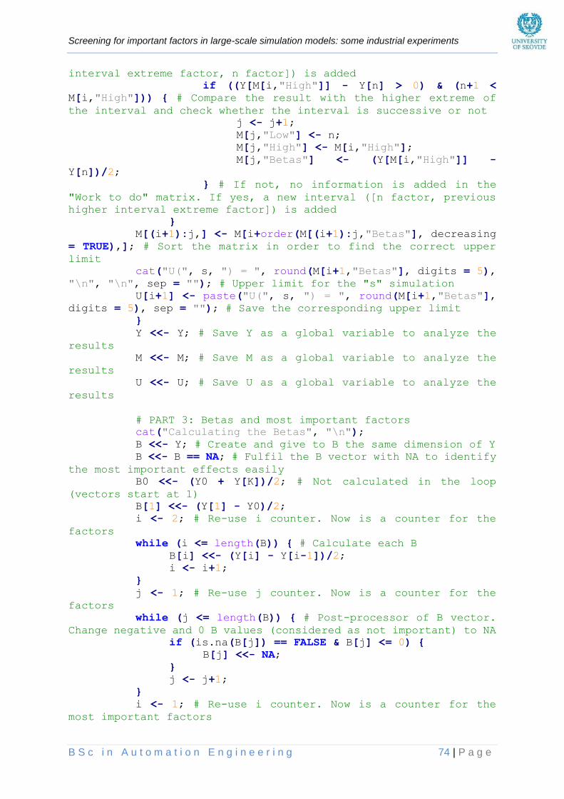
Screening for important factors in large-scale simulation models: some industrial experiments
B S c i n A u t o m a t i o n E n g i n e e r i n g 74 | P a g e
interval extreme factor, n factor]) is added
if ((Y[M[i,"High"]] - Y[n] > 0) & (n+1 <
M[i,"High"])) { # Compare the result with the higher extreme of
the interval and check whether the interval is successive or not
j <- j+1;
M[j,"Low"] <- n;
M[j,"High"] <- M[i,"High"];
M[j,"Betas"] <- (Y[M[i,"High"]] -
Y[n])/2;
} # If not, no information is added in the
"Work to do" matrix. If yes, a new interval ([n factor, previous
higher interval extreme factor]) is added
}
M[(i+1):j,] <- M[i+order(M[(i+1):j,"Betas"], decreasing
= TRUE),]; # Sort the matrix in order to find the correct upper
limit
cat("U(", s, ") = ", round(M[i+1,"Betas"], digits = 5),
"\n", "\n", sep = ""); # Upper limit for the "s" simulation
U[i+1] <- paste("U(", s, ") = ", round(M[i+1,"Betas"],
digits = 5), sep = ""); # Save the corresponding upper limit
}
Y <<- Y; # Save Y as a global variable to analyze the
results
M <<- M; # Save M as a global variable to analyze the
results
U <<- U; # Save U as a global variable to analyze the
results
# PART 3: Betas and most important factors
cat("Calculating the Betas", "\n");
B <<- Y; # Create and give to B the same dimension of Y
B <<- B == NA; # Fulfil the B vector with NA to identify
the most important effects easily
B0 <<- (Y0 + Y[K])/2; # Not calculated in the loop
(vectors start at 1)
B[1] <<- (Y[1] - Y0)/2;
i <- 2; # Re-use i counter. Now is a counter for the
factors
while (i <= length(B)) { # Calculate each B
B[i] <<- (Y[i] - Y[i-1])/2;
i <- i+1;
}
j <- 1; # Re-use j counter. Now is a counter for the
factors
while (j <= length(B)) { # Post-processor of B vector.
Change negative and 0 B values (considered as not important) to NA
if (is.na(B[j]) == FALSE & B[j] <= 0) {
B[j] <<- NA;
}
j <- j+1;
}
i <- 1; # Re-use i counter. Now is a counter for the
most important factors

Screening for important factors in large-scale simulation models: some industrial experiments
B S c i n A u t o m a t i o n E n g i n e e r i n g 75 | P a g e
j <- 0; # Re-use j counter. Now is a counter for the
most important factors
while (i <= length(B)) { # Post-processor of B vector.
Count the number of important factors (B > 0)
if (is.na(B[i]) == FALSE) {
j <- j+1;
k <<- j; # Number of the most important factors
}
i <- i+1;
}
B <<- B; # Save B as a global variable to analyze the
results
cat("Betas calculated", "\n", "\n");
# PART 4: Sub-0 values
OV <- matrix(NA, 1, 2); # Sub-0 values matrix
colnames(OV) <- c("Y0", "B0"); # Re-naming the matrix's
columns
OV[1,"Y0"] <- Y0;
OV[1,"B0"] <- B0;
OV <<- OV; # Save OV as a global variable to analyze the
results
# PART 5: Finishing the function
save.image(file = paste("0. ", MN, "_", S, ".Rdata", sep
= "")); # Save the image to collect the data in case of error
savehistory();
cat("SCREENING SB METHOD FINISHED.", MN, "MODEL", "\n",
"\n");
}
ScreeningI <- function() { # This function is in charge of
doing the SB method, with interactions, running different functions
# PART 1: Scan data & Variables
cat("\n");
cat("SCREENING SB METHOD STARTED.", MN, "MODEL", "\n");
cat("\n");
wb <- loadWorkbook("Inputs.xlsx"); # Read the data from
the excel file
Inputs <<- readWorksheet(wb, sheet = "sheet1", startRow
= 2, colTypes = c(XLC$DATA_TYPE.NUMERIC, XLC$DATA_TYPE.STRING,
XLC$DATA_TYPE.NUMERIC, XLC$DATA_TYPE.NUMERIC), forceConversion =
TRUE); # Creating the variable with the corresponding data-types
K <<- dim(Inputs["Factor"])[1]; # [1] Indicates the
number of rows (K)
s <<- 0; # Counter for the simulations
Y <- matrix(NA, 1+K, 2, byrow = TRUE); # SB objective
function. Include the mirror values
colnames(Y) <- c("Normal", "Mirror"); # Re-naming the
matrix's columns
Y0 <- matrix(NA, 1, 2, byrow = TRUE); # Y matrix for the
0 value (vector and matrix in R start at 1)
colnames(Y0) <- c("Normal", "Mirror"); # Re-naming the
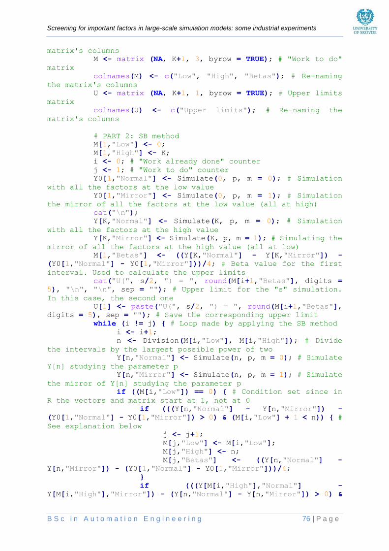
Screening for important factors in large-scale simulation models: some industrial experiments
B S c i n A u t o m a t i o n E n g i n e e r i n g 76 | P a g e
matrix's columns
M <- matrix (NA, K+1, 3, byrow = TRUE); # "Work to do"
matrix
colnames(M) <- c("Low", "High", "Betas"); # Re-naming
the matrix's columns
U <- matrix (NA, K+1, 1, byrow = TRUE); # Upper limits
matrix
colnames(U) <- c("Upper limits"); # Re-naming the
matrix's columns
# PART 2: SB method
M[1,"Low"] <- 0;
M[1,"High"] <- K;
i <- 0; # "Work already done" counter
j <- 1; # "Work to do" counter
Y0[1,"Normal"] <- Simulate(0, p, m = 0); # Simulation
with all the factors at the low value
Y0[1,"Mirror"] <- Simulate(0, p, m = 1); # Simulation
the mirror of all the factors at the low value (all at high)
cat("\n");
Y[K,"Normal"] <- Simulate(K, p, m = 0); # Simulation
with all the factors at the high value
Y[K,"Mirror"] <- Simulate(K, p, m = 1); # Simulating the
mirror of all the factors at the high value (all at low)
M[1,"Betas"] <- ((Y[K,"Normal"] - Y[K,"Mirror"]) -
(Y0[1,"Normal"] - Y0[1,"Mirror"]))/4; # Beta value for the first
interval. Used to calculate the upper limits
cat("U(", s/2, ") = ", round(M[i+1,"Betas"], digits =
5), "\n", "\n", sep = ""); # Upper limit for the "s" simulation.
In this case, the second one
U[1] <- paste("U(", s/2, ") = ", round(M[i+1,"Betas"],
digits = 5), sep = ""); # Save the corresponding upper limit
while (i != j) { # Loop made by applying the SB method
i <- i+1;
n <- Division(M[i,"Low"], M[i,"High"]); # Divide
the intervals by the largest possible power of two
Y[n,"Normal"] <- Simulate(n, p, m = 0); # Simulate
Y[n] studying the parameter p
Y[n,"Mirror"] <- Simulate(n, p, m = 1); # Simulate
the mirror of Y[n] studying the parameter p
if ((M[i,"Low"]) == 0) { # Condition set since in
R the vectors and matrix start at 1, not at 0
if (((Y[n,"Normal"] - Y[n,"Mirror"]) -
(Y0[1,"Normal"] - Y0[1,"Mirror"]) > 0) & (M[i,"Low"] + 1 < n)) { #
See explanation below
j <- j+1;
M[j,"Low"] <- M[i,"Low"];
M[j,"High"] <- n;
M[j,"Betas"] <- ((Y[n,"Normal"] -
Y[n,"Mirror"]) - (Y0[1,"Normal"] - Y0[1,"Mirror"]))/4;
}
if (((Y[M[i,"High"],"Normal"] -
Y[M[i,"High"],"Mirror"]) - (Y[n,"Normal"] - Y[n,"Mirror"]) > 0) &
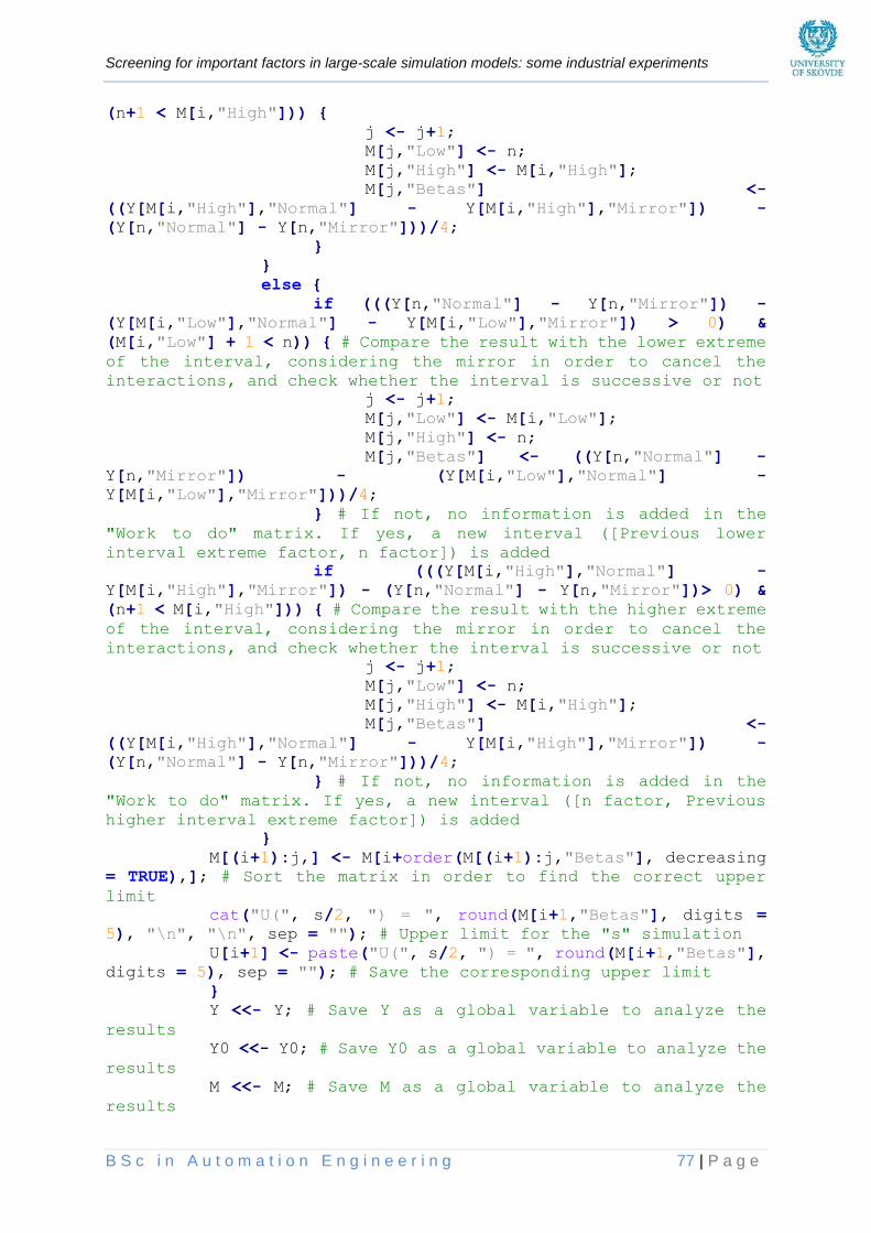
Screening for important factors in large-scale simulation models: some industrial experiments
B S c i n A u t o m a t i o n E n g i n e e r i n g 77 | P a g e
(n+1 < M[i,"High"])) {
j <- j+1;
M[j,"Low"] <- n;
M[j,"High"] <- M[i,"High"];
M[j,"Betas"] <-
((Y[M[i,"High"],"Normal"] - Y[M[i,"High"],"Mirror"]) -
(Y[n,"Normal"] - Y[n,"Mirror"]))/4;
}
}
else {
if (((Y[n,"Normal"] - Y[n,"Mirror"]) -
(Y[M[i,"Low"],"Normal"] - Y[M[i,"Low"],"Mirror"]) > 0) &
(M[i,"Low"] + 1 < n)) { # Compare the result with the lower extreme
of the interval, considering the mirror in order to cancel the
interactions, and check whether the interval is successive or not
j <- j+1;
M[j,"Low"] <- M[i,"Low"];
M[j,"High"] <- n;
M[j,"Betas"] <- ((Y[n,"Normal"] -
Y[n,"Mirror"]) - (Y[M[i,"Low"],"Normal"] -
Y[M[i,"Low"],"Mirror"]))/4;
} # If not, no information is added in the
"Work to do" matrix. If yes, a new interval ([Previous lower
interval extreme factor, n factor]) is added
if (((Y[M[i,"High"],"Normal"] -
Y[M[i,"High"],"Mirror"]) - (Y[n,"Normal"] - Y[n,"Mirror"])> 0) &
(n+1 < M[i,"High"])) { # Compare the result with the higher extreme
of the interval, considering the mirror in order to cancel the
interactions, and check whether the interval is successive or not
j <- j+1;
M[j,"Low"] <- n;
M[j,"High"] <- M[i,"High"];
M[j,"Betas"] <-
((Y[M[i,"High"],"Normal"] - Y[M[i,"High"],"Mirror"]) -
(Y[n,"Normal"] - Y[n,"Mirror"]))/4;
} # If not, no information is added in the
"Work to do" matrix. If yes, a new interval ([n factor, Previous
higher interval extreme factor]) is added
}
M[(i+1):j,] <- M[i+order(M[(i+1):j,"Betas"], decreasing
= TRUE),]; # Sort the matrix in order to find the correct upper
limit
cat("U(", s/2, ") = ", round(M[i+1,"Betas"], digits =
5), "\n", "\n", sep = ""); # Upper limit for the "s" simulation
U[i+1] <- paste("U(", s/2, ") = ", round(M[i+1,"Betas"],
digits = 5), sep = ""); # Save the corresponding upper limit
}
Y <<- Y; # Save Y as a global variable to analyze the
results
Y0 <<- Y0; # Save Y0 as a global variable to analyze the
results
M <<- M; # Save M as a global variable to analyze the
results

Screening for important factors in large-scale simulation models: some industrial experiments
B S c i n A u t o m a t i o n E n g i n e e r i n g 78 | P a g e
U <<- U; # Save U as a global variable to analyze the
results
# PART 3: Betas and most important factors
cat("Calculating the Betas", "\n");
B <<- c(1:(K)); # Vector in which the B values are saved
B <<- B == NA; # Fulfil the B vector with NA to identify
the most important effects easily
B[1] <<- ((Y[1,"Normal"] - Y[1,"Mirror"]) -
(Y0[1,"Normal"] - Y0[1,"Mirror"]))/4;
i <- 2; # Re-use i counter. Now is a counter for the
factors
while (i <= length(B)) { # Calculate each B
B[i] <<- ((Y[i,"Normal"] - Y[i,"Mirror"]) - (Y[i-
1,"Normal"] - Y[i-1,"Mirror"]))/4
i <- i+1;
}
j <- 1; # Re-use j counter. Now is a counter for the
factors
while (j <= length(B)) { # Post-processor of B vector.
Change negative and 0 B values (considered as not important) to NA
if (is.na(B[j]) == FALSE & B[j] <= 0) {
B[j] <<- NA;
}
j <- j+1;
}
i <- 1; # Re-use j counter. Now is a counter for the
most important factors
j <- 0; # Re-use j counter. Now is a counter for the
most important factors
while (i <= length(B)) { # Post-processor of B vector.
Count the number of important factors (B > 0)
if (is.na(B[i]) == FALSE) {
j <- j+1;
k <<- j; # Number of the most important factors
}
i <- i+1;
}
B <<- B; # Save B as a global variable to analyze the
results
cat("Betas calculated", "\n", "\n");
# PART 4: Interactions
cat("Calculating the interactions", "\n");
cat("\n");
li <- 10; # Set manually in 10 to select the reduce the
time of the whole simulation
Interactions <- 0; # Variable that sum all the
interactions
Limit <- B[order(B, decreasing = TRUE)[li]]; # Limit of
the most important factor for calculating their interactions
while (is.na(Limit) == TRUE) { # Updating the limits
according with the limit variable

Screening for important factors in large-scale simulation models: some industrial experiments
B S c i n A u t o m a t i o n E n g i n e e r i n g 79 | P a g e
li <- li-1;
Limit <- B[order(B, decreasing = TRUE)[li]];
}
Bi <- matrix(0, K, K, byrow = TRUE); # Interactions
matrix
Biplot <- matrix(NA, (li*(li-1))/2, 2, byrow = TRUE); #
Interactions matrix for the plotting
colnames(Biplot) <- c("Name", "Interaction"); # Re-
naming the matrix' columns
J <- 1; # Counter for the Biplot variable
for (i in 1:(K-1)) { # Interaction to calculate (two-
factors interaction) . Variable i re-used. Counter for the
interactions (j)
for (j in (i+1):K) { # Variable j re-used. Counter
for the interactions (j')
if(is.na(B[i]) == FALSE & is.na(B[j]) == FALSE
& B[i] >= Limit & B[j] >= Limit) {
if (i+1 == j) { # Consecutive
interactions
Y11 <- Y[j];
Y10 <- Y[i];
Y01 <- Simulate(i-1, p, c = j);
# For Y00 we need to find the last
value calculated, as follows
k <- i; # Variable for each Y[j].
Re-used
a <- 3; # Variable for the loop
while (a != 15 & k != 1) {
if (is.na(Y[k-1]) == FALSE) {
Y00 <- Y[k-1];
a <- 15;
}
k <- k-1;
}
if ((k == 1)) { # Condition for the
Y0 value
Y00 <- Y0[,"Normal"];
}
}
else {
Y11 <- Simulate(i, p, c = j);
Y10 <- Y[i];
Y01 <- Simulate(i-1, p, c = j);
# For Y00 we need to find the last
value calculated, as follows
k <- i; # Variable for each Y[j].
Re-used
a <- 3; # Variable for the loop
while (a != 15 & k != 1) {
if (is.na(Y[k-1]) == FALSE) {
Y00 <- Y[k-1];
a <- 15;
}

Screening for important factors in large-scale simulation models: some industrial experiments
B S c i n A u t o m a t i o n E n g i n e e r i n g 80 | P a g e
k <- k-1;
}
if ((k == 1)) { # Condition for the
Y0 value
Y00 <- Y0[,"Normal"];
}
}
Bi[i,j] <- ((Y11 + Y00) - (Y10 + Y01))/4;
# Interaction calculated
Biplot[J,"Interaction"] <- Bi[i,j];
Biplot[J,"Name"] <- paste(Inputs[i,
"Name"], "&", Inputs[j, "Name"]);
Biplot <-
Biplot[order(Biplot[,"Interaction"], decreasing = TRUE),]; #
Biplot variable ordered by importance
J <- J+1;
Interactions <- Interactions + Bi[i,j];
# Sum of the interactions
cat("Interaction [", i, ",", j, "]
calculated", "\n", "\n", sep = "");
}
}
}
Bi <<- Bi; # Save Biplot as a global variable to analyze
the results
Biplot <<- Biplot; # Save Biplot as a global variable to
analyze the results
cat("Interactions calculated", "\n", "\n");
#PART 5: Sub-0 values
B0 <<- (Y0[1] + Y[K] - 2*Interactions)/2; # Calculated
here because needs the interactions. Approximated value
OV <- matrix(NA, 1, 3); # Sub-0 values matrix
colnames(OV) <- c("Y0", "Y0 mirror", "B0");
OV[1,"Y0"] <- Y0[1];
OV[1,"Y0 mirror"] <- Y0[2];
OV[1,"B0"] <- B0;
OV <<- OV; # Save OV as a global variable to analyze the
results
# PART 5: Finishing the function
save.image(file = paste("0. ", MN, "_", S, ".Rdata", sep
= "")); # Save the image to collect the data in case of error
savehistory();
cat("SCREENING SB METHOD FINISHED.", MN, "MODEL", "\n",
"\n");
}
ParetoPoint <- function(p, ...) { # This function is in charge
of simulating the factors for the Pareto chart
# PART 1: Inputs for the simulation
s <<- s+1; # Simulations counter
to <- proc.time(); # Variable needed to calculate the
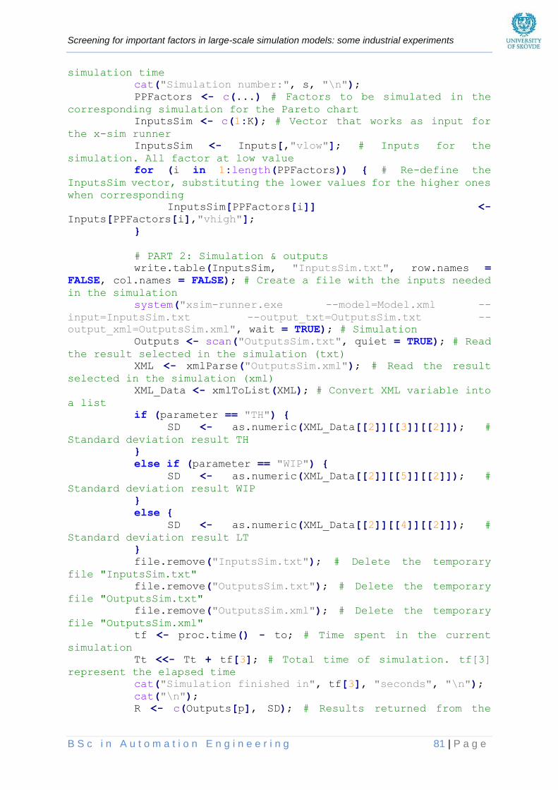
Screening for important factors in large-scale simulation models: some industrial experiments
B S c i n A u t o m a t i o n E n g i n e e r i n g 81 | P a g e
simulation time
cat("Simulation number:", s, "\n");
PPFactors <- c(...) # Factors to be simulated in the
corresponding simulation for the Pareto chart
InputsSim <- c(1:K); # Vector that works as input for
the x-sim runner
InputsSim <- Inputs[,"vlow"]; # Inputs for the
simulation. All factor at low value
for (i in 1:length(PPFactors)) { # Re-define the
InputsSim vector, substituting the lower values for the higher ones
when corresponding
InputsSim[PPFactors[i]] <-
Inputs[PPFactors[i],"vhigh"];
}
# PART 2: Simulation & outputs
write.table(InputsSim, "InputsSim.txt", row.names =
FALSE, col.names = FALSE); # Create a file with the inputs needed
in the simulation
system("xsim-runner.exe --model=Model.xml --
input=InputsSim.txt --output_txt=OutputsSim.txt --
output_xml=OutputsSim.xml", wait = TRUE); # Simulation
Outputs <- scan("OutputsSim.txt", quiet = TRUE); # Read
the result selected in the simulation (txt)
XML <- xmlParse("OutputsSim.xml"); # Read the result
selected in the simulation (xml)
XML_Data <- xmlToList(XML); # Convert XML variable into
a list
if (parameter == "TH") {
SD <- as.numeric(XML_Data[[2]][[3]][[2]]); #
Standard deviation result TH
}
else if (parameter == "WIP") {
SD <- as.numeric(XML_Data[[2]][[5]][[2]]); #
Standard deviation result WIP
}
else {
SD <- as.numeric(XML_Data[[2]][[4]][[2]]); #
Standard deviation result LT
}
file.remove("InputsSim.txt"); # Delete the temporary
file "InputsSim.txt"
file.remove("OutputsSim.txt"); # Delete the temporary
file "OutputsSim.txt"
file.remove("OutputsSim.xml"); # Delete the temporary
file "OutputsSim.xml"
tf <- proc.time() - to; # Time spent in the current
simulation
Tt <<- Tt + tf[3]; # Total time of simulation. tf[3]
represent the elapsed time
cat("Simulation finished in", tf[3], "seconds", "\n");
cat("\n");
R <- c(Outputs[p], SD); # Results returned from the
Screening for important factors in large-scale simulation models: some industrial experiments
B S c i n A u t o m a t i o n E n g i n e e r i n g 82 | P a g e
simulation
return(R); # Simulation result
}
Simulate <- function(n, p, m = 0, c = 0) { # This function is
the one that simulates the inputs of the system
# PART 1: Variables & simulation information
s <<- s+1; # Simulations counter
to <- proc.time(); # Variable needed to calculate the
simulation time
cat("Simulation number:", s, "\n");
if (m == 0) { # m determines whether the simulation is
for the mirror (m = 1) or not (m = 0)
if (c == 0) { # c determines whether the current
simulation is for calculating the interactions (c != 0) or not (c
= 0)
cat("Simulating Y[", n,"]", "\n", sep = "");
# For example, Y[15] means that the first 15 factors are set at
the high value and the rest with the low value
}
else {
cat("Simulating Y[", n, ",", c, "]", "\n", sep
= ""); # For example, Y[3,15] means that the first 3 factors are
set at the high value and the rest, except the 15th, with the low
value
}
}
else {
cat("Simulating mirror Y[", n,"]", "\n", sep = "");
# For example, Y[15] (mirror) means that the first 15 factors
are set at the low value and the rest with the high value
}
n <- n+1;
InputsSim <- c(1:K);
# PART 2: Inputs for the simulation
if (m == 0) {
InputsSim <- Inputs[,"vhigh"]; # Inputs for the
simulation
while (n <= K) { # Re-define the InputsSim vector,
substituting the higher values for the lower ones when
corresponding
InputsSim[n] <- Inputs[n,"vlow"];
n <- n+1;
}
}
else {
InputsSim <- Inputs[,"vlow"]; # Inputs for the
simulation of the mirror
while (n <= K) { # Re-define the InputsSim vector,
substituting the lower values for the higher ones when
corresponding
InputsSim[n] <- Inputs[n,"vhigh"];
Screening for important factors in large-scale simulation models: some industrial experiments
B S c i n A u t o m a t i o n E n g i n e e r i n g 83 | P a g e
n <- n+1;
}
}
if (c != 0) {
InputsSim[c] <- Inputs[c,"vhigh"];
}
# PART 3: Simulation & outputs
write.table(InputsSim, "InputsSim.txt", row.names =
FALSE, col.names = FALSE); # Create a file with the inputs needed
in the simulation
system("xsim-runner.exe --model=Model.xml --
input=InputsSim.txt --output_txt=OutputsSim.txt", wait = TRUE); #
Simulation
Outputs <- scan("OutputsSim.txt", quiet = TRUE); # Read
the result selected in the simulation
file.remove("InputsSim.txt"); # Delete the temporary
file "InputsSim.txt"
file.remove("OutputsSim.txt"); # Delete the temporary
file "OutputsSim.txt"
tf <- proc.time() - to; # Time spent in the current
simulation
Tt <<- Tt + tf[3]; # Total time of simulation. tf[3]
represent the elapsed time
cat("Simulation finished in", tf[3], "seconds", "\n");
R <- Outputs[p]; # Simulation result
return(R); # Return the result
}
Division <- function(x,y) { #In this function, the largest
possible power of two is calculated to divide the groups properly
pot <- 0;
k <- 0;
while (y - x > pot) {
k <- k+1;
pot <- 2^k;
}
R <- 2^(k-1)+x; # Result of the calculation
return(R); # Return the result
}
#©Ragm93&JmgsA A A A A A A A A A A A A AA A A A A A A A A A A A A A A A A A A A A A A A A A A A A A A A A A A A A A A A A A A A A A A A A A A A A A A A A A A A A A A A A A A A A A A A A A A A A A A A A A A A A A A A A A A A A A A A A A A A A A A A A A A A A A A A A A A A A A A A A A A A A A A A A A A A A A A A A A A A A A A A A A A A A A A A A A A A A A A A A A A A A A A A A A A A A A A A A A A A A A A A A A A A A A A A A A A A A A A A A A A A A A A A
A A A A A A A A A A A A A A A A A A A A A A A A A A A A A A A A A A A A A A A A A A A A A A A A A A A A A A A A A A A A A A A A A A A A A A A A A A A A A A A A A A A A A A A A A A A A A A A A A A A A A A A A A A A A A A A A A A A A A A A A A A A A A A A A A A A A A A A A A A A A A A A A A A A A A A A A A A A A A A A A A A A A A A A A A A A A A A A A A A A A A A A A A A A A A A A A A A A A A A A A A A A A A A A A A A A A A A A A A A A A A A A A A A A A A A A A A A A A A A A A A A A A A A A A A A A A A A A A A A A A A A A A A A A A A A A A A A A A A A A A A A A A A A A A A A A A A A A A A A A A A A A A A A A A A A A A A A A A A A A A A A A A A A A A A A A A A A A A A A A A A A A A A A A A A A A A A A A A A A A A A A A A A A A A A A A A A A A A A A
A A A A A A A A A A A A A A A A A A A A A A A A A A A A A A A A A A A A A A A A A A A A A A A A A A A A A A A A A A A A A A A A A A A A A A A A A A A A A A A A A A A A A A A A A A A A A A A A A A A A A A A A A A A A A A A A A A A A A A A A A A A A A A A A A A A A A A A A A A A A A A A A A A A A A A A A A A A A A A A A A A A A A A A A A A A A A A A A A A A A A A A A A A A A A A A A A A A A A A A A A A A A A A A A A A A A A A A A A A A A A A A A A A A A A A A A A A A A A A A A A A A A A A A A A A A A A A A A A A A A A A A A A A A A A A A A A A A A A A A A A A A A A A A A A A A A A A A A A A A A A A A A A A A A A A A A A A A A A A A A A A A A A A A A A A A A A A A A A A A A A A A A A A A A A A A A A A A A A A A A A A A A A A A A A A A A A A A A A A
A A A A A A A A A A A A A A A A A A A A A A A A A A A A A A A A A A A A A A A A A A A A A A A A A A A A A A A A A A A A A A A A A A A A A A A A A A A A A A A A A A A A A A A A A A A A A A A A A A A A A A A A A A A A A A A A A A A A A A A A A A A A A A A A A A A A A A A A A A A A A A A A A A A A A A A A A A A A A A A A A A A A A A A A A A A A A A A A A A A A A A A A A A A A A A A A A A A A A A A A A A A A A A A A A A A A A A A A A A A A A A A A A A A A A A A A A A A A A A A A A A A A A A A A A A A A A A A A A A A A A A A A A A A A A A A A A A A A A A A A A A A A A A A A A A A A A A A A A A A A A A A A A A A A A A A A A A A A A A A A A A A A A A A A A A A A A A A A A A A A A A A A A A A A A A A A A A A A A A A A A A A A A A A A A A A A A A A A A A
A A A A A A A A A A A A A A A A A A A A A A A A A A A A A A A A A A A A A A A A A A A A A A A A A A A A A A A A A A A A A A A A A A A A A A A A A A A A A A A A A A A A A A A A A A A A A A A A A A A A A A A A A A A A A A A A A A A A A A A A A A A A A A A A A A A A A A A A A A A A A A A A A A A A A A A A A A A A A A A A A A A A A A A A A A A A A A A A A A A A A A A A A A A A A A A A A A A A A A A A A A A A A A A A A A A A A A A A A A A A A A A A A A A A A A A A A A A A A A A A A A A A A A A A A A A A A A A A A A A A A A A A A A A A A A A A A A A A A A A A A A A A A A A A A A A A A A A A A A A A A A A A A A A A A A A A A A A A A A A A A A A A A A A A A A A A A A A A A A A A A A A A A A A A A A A A A A A A A A A A A A A A A A A A A A A A A A A A A A
A
A A A A A A A A A A A A A A A A A A A A A A A A A A A A A A A A A A A A A A A A A A A A A A A A A A A A A A A A A A A A A A A A A A A A A A A A A A A A A A A A A A A A A A A A A A A A A A A A A A A A A A A A A A A A A A A A A A A A A A A A A A A A A A A A A A A A A A A A A A A A A A A A A A A A A A A A A A A A A A A A A A A A A A A A A A A A A A A A A A A A A A A A A A A A A A A A A A A A A A A A A A A A A A A A A A A A A A A A A A A A A A A A A A A A A A A A A A A A A A A A A A A A A A A A A A A A A A A A A A A A A A A A A A A A A A A A A A A A A A A A A A A A A A A A A A A A A A A A A A A A A A A A A A A A A A A A A A A A A A A A A A A A A A A A A A A A A A A A A A A A A A A A A A A A A A A A A A A A A A A A A A A A A A A A A A A A A A A A A A
A A A A A A A A A A A A A A A A A A A A A A A A A A A A A A A A A A A A A A A A A A A A A A A A A A A A A A A A A A A A A A A A A A A A A A A A A A A A A A A A A A A A A A A A A A A A A A A A A A A A A A A A A A A A A A A A A A A A A A A A A A A A A A A A A A A A A A A A A A A A A A A A A A A A A A A A A A A A A A A A A A A A A A A A A A A A A A A A A A A A A A A A A A A A A A A A A A A A A A A A A A A A A A A A A A A A A A A A A A A A A A A A A A A A A A A A A A A A A A A A A A A A A A A A A A A A A A A A A A A A A A A A A A A A A A A A A A A A A A A A A A A A A A A A A A A A A A A A A A A A A A A A A A A A A A A A A A A A A A A A A A A A A A A A A A A A A A A A A A A A A A A A A A A A A A A A A A A A A A A A A A A A A A A A A A A A A A A A A A
A A A A A A A A A A A A A A A A A A A A A A A A A A A A A A A A A A A A A A A A A A A A A A A A A A A A A A A A A A A A A A A A A A A A A A A A A A A A A A A A A A A A A A A A A A A A A A A A A A A A A A A A A A A A A A A A A A A A A A A A A A A A A A A A A A A A A A A A A A A A A A A A A A A A A A A A A A A A A A A A A A A A A A A A A A A A A A A A A A A A A A A A A A A A A A A A A A A A A A A A A A A A A A A A A A A A A A A A A A A A A A A A A A A A A A A A A A A A A A A A A A A A A A A A A A A A A A A A A A A A A A A A A A A A A A A A A A A A A A A A A A A A A A A A A A A A A A A A A A A A A A A A A A A A A A A A A A A A A A A A A A A A A A A A A A A A A A A A A A A A A A A A A A A A A A A A A A A A A A A A A A A A A A A A A A A A A A A A A A
A A A A A A A A A A A A A A A A A A A A A A A A A A A A A A A A A A A A A A A A A A A A A A A A A A A A A A A A A A A A A A A A A A A A A A A A A A A A A A A A A A A A A A A A A A A A A A A A A A A A A A A A A A A A A A A A A A A A A A A A A A A A A A A A A A A A A A A A A A A A A A A A A A A A A A A A A A A A A A A A A A A A A A A A A A A A A A A A A A A A A A A A A A A A A A A A A A A A A A A A A A A A A A A A A A A A A A A A A A A A A A A A A A A A A A A A A A A A A A A A A A A A A A A A A A A A A A A A A A A A A A A A A A A A A A A A A A A A A A A A A A A A A A A A A A A A A A A A A A A A A A A A A A A A A A A A A A A A A A A A A A A A A A A A A A A A A A A A A A A A A A A A A A A A A A A A A A A A A A A A A A A A A A A A A A A A A A A A A A
A A A A A A A A A A A A A A A A A A A A A A A A A A A A A A A A A A A A A A A A A A A A A A A A A A A A A A A A A A A A A A A A A A A A A A A A A A A A A A A A A A A A A A A A A A A A A A A A A A A A A A A A A A A A A A A A A A A A A A A A A A A A A A A A A A A A A A A A A A A A A A A A A A A A A A A A A A A A A A A A A A A A A A A A A A A A A A A A A A A A A A A A A A A A A A A A A A A A A A A A A A A A A A A A A A A A A A A A A A A A A A A A A A A A A A A A A A A A A A A A A A A A A A A A A A A A A A A A A A A A A A A A A A A A A A A A A A A A A A A A A A A A A A A A A A A A A A A A A A A A A A A A A A A A A A A A A A A A A A A A A A A A A A A A A A A A A A A A A A A A A A A A A
#OTHER FUNCTIONS USED IN THE PRESENT PROJECT
Pareto_OPT <- function(p, Name, ...) { # This function is in
charge of calculating the Pareto graph, necessary to compare with
the optimization study
# PART 1: Variables & Simulation information
cat("\n");
cat("PARETO GRAPH CALCULATIONS", "\n");
cat("\n");
PFactors <- c(...); # Most important factors ordered by

Screening for important factors in large-scale simulation models: some industrial experiments
B S c i n A u t o m a t i o n E n g i n e e r i n g 84 | P a g e
importance
ResultPareto <- matrix(NA, length(PFactors)+1, 7); #
Matrix for the Pareto simulations' results
colnames(ResultPareto) <- c("Result", "SD", "Lower",
"Upper", "SE", "Upper_SE", "Lower_SE"); # Re-naming the columns of
the matrix
cat("Pareto simulations initialized", "\n", "\n", sep =
"");
# PART 2: Pareto simulations
cat("Pareto simulation: 1/", length(PFactors)+1, "\n",
sep = "");
R <- ParetoPoint(p); # First simulation
ResultPareto[1,"Result"] <- R[1];
ResultPareto[1,"SD"] <- R[2];
ResultPareto[1,"Upper"] <- ResultPareto[1,"Result"] +
ResultPareto[1,"SD"]; # Lower value for the confidence interval
ResultPareto[1,"Lower"] <- ResultPareto[1,"Result"] -
ResultPareto[1,"SD"]; # Higher value for the confidence interval
ResultPareto[1,"SE"] <- qt((1-alpha/2), df = (n-
1))*(ResultPareto[1,"SD"]/sqrt(n)); # Standard error for each
variable
ResultPareto[1,"Upper_SE"] <- ResultPareto[1,"Result"]
+ ResultPareto[1,"SE"]; # Lower value for the standard error
ResultPareto[1,"Lower_SE"] <- ResultPareto[1,"Result"]
- ResultPareto[1,"SE"]; # Higher value for the standard error
for (i in 1:(length(PFactors))) { # Pareto simulations
of the most important factors
cat("Pareto simulation: ", i+1, "/",
length(PFactors)+1, "\n", sep = "");
R <- ParetoPoint(p, PFactors[1:i]);
ResultPareto[i+1,"Result"] <- R[1];
ResultPareto[i+1,"SD"] <- R[2];
ResultPareto[i+1,"Upper"] <-
ResultPareto[i+1,"Result"] + ResultPareto[i+1,"SD"];
ResultPareto[i+1,"Lower"] <-
ResultPareto[i+1,"Result"] - ResultPareto[i+1,"SD"];
ResultPareto[i+1,"SE"] <- qt((1-alpha/2), df = (n-
1))*(ResultPareto[i+1,"SD"]/sqrt(n));
ResultPareto[i+1,"Upper_SE"] <-
ResultPareto[i+1,"Result"] + ResultPareto[i+1,"SE"];
ResultPareto[i+1,"Lower_SE"] <-
ResultPareto[i+1,"Result"] - ResultPareto[i+1,"SE"];
}
cat("Pareto simulations finished", "\n", "\n", sep =
"");
# PART 3: Data frame for the graphics
Changes <- 0:(length(PFactors)); # x axis
y <- ResultPareto[,"Result"]; # y axis
Upper <- ResultPareto[,"Upper"]; # Higher value for the
confidence interval
Lower <- ResultPareto[,"Lower"]; # Lower value for the

Screening for important factors in large-scale simulation models: some industrial experiments
B S c i n A u t o m a t i o n E n g i n e e r i n g 85 | P a g e
confidence interval
SD <- ResultPareto[,"SD"]; # Standard deviation results
SE <- ResultPareto[,"SE"]; # Standard error results
Upper_SE <- ResultPareto[,"Upper_SE"]; # Higher value
for the standard error
Lower_SE <- ResultPareto[,"Lower_SE"]; # Lower value for
the standard error
Plot_data_Pareto_OPT <<- data.frame(Name, Changes, y,
SD, Upper, Lower, SE, Upper_SE, Lower_SE); # Data frame with all
the data to plot
Plot_data_Pareto_SB_OPT <<- Plot_data_Pareto_OPT; # Data
frame with all the data to plot (SB_OPT chart)
# PART 4: Pareto graph Optimization. Standard error
Graph_Pareto_OPT <<- ggplot(Plot_data_Pareto_OPT, aes(x
= Changes, y = y)); # Creating the graph
Graph_Pareto_OPT <<- Graph_Pareto_OPT + geom_line(stat
= "identity", colour = "blue") + geom_point(colour = "red") +
geom_ribbon(aes(ymax = Upper_SE, ymin = Lower_SE), alpha = 0.15);
# Main layers of the graph
Graph_Pareto_OPT <<- Graph_Pareto_OPT +
ggtitle(paste("OPTIMIZATION", MN, "MODEL: PARETO GRAPH")) + labs(x
= "Changes", y = parameter, colour = "", fill = "") +
scale_x_discrete(limits = Changes, labels = Changes) +
geom_text(aes(label = Name, angle = -90, y = y-0.005,
hjust = 0), colour = "green", size = 4) +
theme(text = element_text(size = 20), plot.title =
element_text(size = 25, face = "bold"), axis.text.x =
element_text(colour = "blue", size = 11, angle = 0, vjust = 0),
axis.text.y = element_text(colour = "blue", size = 11, angle = 0,
hjust = 0),
axis.line = element_line(colour = "black"),
panel.background = element_blank(), panel.grid.major =
element_blank(), panel.grid.minor = element_blank(),
legend.position = "none"); # Aesthetic layers added to the main
chart
# PART 5: Pareto graph Optimization. Confidence interval
Graph_Pareto_CI_OPT <<- ggplot(Plot_data_Pareto_OPT,
aes(x = Changes, y = y)); # Creating the graph
Graph_Pareto_CI_OPT <<- Graph_Pareto_CI_OPT +
geom_line(stat = "identity", colour = "blue") + geom_point(colour
= "red") + geom_ribbon(aes(ymax = Upper, ymin = Lower), alpha =
0.15); # Main layers of the graph
Graph_Pareto_CI_OPT <<- Graph_Pareto_CI_OPT +
ggtitle(paste("OPTIMIZATION", MN, "MODEL: PARETO GRAPH (MaxMin)"))
+ labs(x = "Changes", y = parameter, colour = "", fill = "") +
scale_x_discrete(limits = Changes, labels = Changes) +
geom_text(aes(label = Name, angle = -90, y = y-0.005,
hjust = 0), colour = "green", size = 4) +
theme(text = element_text(size = 20), plot.title =
element_text(size = 25, face = "bold"), axis.text.x =
element_text(colour = "blue", size = 11, angle = 0, vjust = 0),
Screening for important factors in large-scale simulation models: some industrial experiments
B S c i n A u t o m a t i o n E n g i n e e r i n g 86 | P a g e
axis.text.y = element_text(colour = "blue", size = 11, angle = 0,
hjust = 0),
axis.line = element_line(colour = "black"),
panel.background = element_blank(), panel.grid.major =
element_blank(), panel.grid.minor = element_blank(),
legend.position = "none"); # Aesthetic layers added to the main
chart
# PART 6: Mixing SB and OPT graphs (especially performed
to the VCC_ASSEMBLY model)
# Generating the main graph (SE)
Graph_Pareto_SB_OPT <<- ggplot(); # Creating the graph
Graph_Pareto_SB_OPT <<- Graph_Pareto_SB_OPT +
geom_line(data = Plot_data_Pareto_SB_OPT, aes(x = Changes, y = y),
stat = "identity", colour = "blue") +
geom_point(data = Plot_data_Pareto_SB_OPT, aes(x =
Changes, y = y), colour = "blue") + geom_ribbon(data =
Plot_data_Pareto_SB_OPT, aes(x = Changes, y = y, ymax = Upper_SE,
ymin = Lower_SE), fill = "blue", alpha = 0.15); # Main layers of
the graph
Graph_Pareto_SB_OPT <<- Graph_Pareto_SB_OPT +
ggtitle(paste("SB-OPTIMIZATION", MN, "MODEL: PARETO GRAPH")) +
labs(x = "Changes", y = parameter, colour = "", fill = "") +
scale_x_discrete(limits = Changes, labels = Changes) +
geom_text(data = Plot_data_Pareto_SB_OPT, aes(label =
Name, angle = 90, x = Changes, y = y+0.5, hjust = 0), colour =
"blue", size = 4) + annotate(geom = "text", x = length(Changes)-1,
y = Plot_data_Pareto_SB_OPT[1,"y"], label = "SB", size = 8,
fontface = "bold", colour = "red") +
annotate(geom = "text", x = length(Changes)-1, y =
Plot_data_Pareto_SB_OPT[1,"y"]-Plot_data_Pareto_SB_OPT[1,"y"]/20,
label = "OPT", size = 8, fontface = "bold", colour = "blue") +
annotate(geom = "text", x = length(Changes)-1, y =
Plot_data_Pareto_SB_OPT[1,"y"]*1.9, label = "", colour = "white")
+
theme(text = element_text(size = 20), plot.title =
element_text(size = 25, face = "bold"), axis.text.x =
element_text(colour = "blue", size = 11, angle = 0, vjust = 0),
axis.text.y = element_text(colour = "blue", size = 11, angle = 0,
hjust = 0),
axis.line = element_line(colour = "black"),
panel.background = element_blank(), panel.grid.major =
element_blank(), panel.grid.minor = element_blank(),
legend.position = "none"); # Aesthetic layers added to the main
chart
# Generating the main graph (MM)
Graph_Pareto_CI_SB_OPT <<- ggplot(); # Creating the
graph
Graph_Pareto_CI_SB_OPT <<- Graph_Pareto_CI_SB_OPT +
geom_line(data = Plot_data_Pareto_SB_OPT, aes(x = Changes, y = y),
stat = "identity", colour = "blue") +
geom_point(data = Plot_data_Pareto_SB_OPT, aes(x =
Changes, y = y), colour = "blue") + geom_ribbon(data =
Screening for important factors in large-scale simulation models: some industrial experiments
B S c i n A u t o m a t i o n E n g i n e e r i n g 87 | P a g e
Plot_data_Pareto_SB_OPT, aes(x = Changes, y = y, ymax = Upper_SE,
ymin = Lower_SE), fill = "blue", alpha = 0.15); # Main layers of
the graph
Graph_Pareto_CI_SB_OPT <<- Graph_Pareto_CI_SB_OPT +
ggtitle(paste("SB-OPTIMIZATION", MN, "MODEL: PARETO GRAPH
(MaxMin)")) + labs(x = "Changes", y = parameter, colour = "", fill
= "") + scale_x_discrete(limits = Changes, labels = Changes) +
geom_text(data = Plot_data_Pareto_SB_OPT, aes(label =
Name, angle = 90, x = Changes, y = y+0.5, hjust = 0), colour =
"blue", size = 4) + annotate(geom = "text", x = length(Changes)-
1, y = Plot_data_Pareto_SB_OPT[1,"y"], label = "SB", size = 8,
fontface = "bold", colour = "red") +
annotate(geom = "text", x = length(Changes)-1, y =
Plot_data_Pareto_SB_OPT[1,"y"]-Plot_data_Pareto_SB_OPT[1,"y"]/20,
label = "OPT", size = 8, fontface = "bold", colour = "blue") +
annotate(geom = "text", x = length(Changes)-1, y =
Plot_data_Pareto_SB_OPT[1,"y"]*1.9, label = "", colour = "white")
+
theme(text = element_text(size = 20), plot.title =
element_text(size = 25, face = "bold"), axis.text.x =
element_text(colour = "blue", size = 11, angle = 0, vjust = 0),
axis.text.y = element_text(colour = "blue", size = 11, angle = 0,
hjust = 0),
axis.line = element_line(colour = "black"),
panel.background = element_blank(), panel.grid.major =
element_blank(), panel.grid.minor = element_blank(),
legend.position = "none"); # Aesthetic layers added to the main
chart
# Mixing SE graphs
Plot_data_Pareto_SB_OPT[,"y"] <-
Plot_data_Pareto[1:length(Changes),"y"];
Plot_data_Pareto_SB_OPT[,"Name"] <-
Plot_data_Pareto[1:length(Changes),"Name"];
Plot_data_Pareto_SB_OPT[,"Upper_SE"] <-
Plot_data_Pareto[1:length(Changes),"Upper_SE"];
Plot_data_Pareto_SB_OPT[,"Lower_SE"] <-
Plot_data_Pareto[1:length(Changes),"Lower_SE"];
Graph_Pareto_SB_OPT <<- Graph_Pareto_SB_OPT +
geom_line(data = Plot_data_Pareto_SB_OPT, aes(x = Changes, y = y),
stat = "identity", colour = "red") + geom_point(data =
Plot_data_Pareto_SB_OPT, aes(x = Changes, y = y), colour = "red")
+
geom_ribbon(data = Plot_data_Pareto_SB_OPT, aes(x =
Changes, y = y, ymax = Upper_SE, ymin = Lower_SE), fill = "red",
alpha = 0.15) + geom_text(data = Plot_data_Pareto_SB_OPT, aes(label
= Name, angle = -90, x = Changes, y = y-0.5, hjust = 0), colour =
"red", size = 4)
# Mixing MM graphs
Plot_data_Pareto_SB_OPT[,"Upper"] <-
Plot_data_Pareto[1:length(Changes),"Upper"];
Plot_data_Pareto_SB_OPT[,"Lower"] <-
Plot_data_Pareto[1:length(Changes),"Lower"];
Graph_Pareto_CI_SB_OPT <<- Graph_Pareto_CI_SB_OPT +

Screening for important factors in large-scale simulation models: some industrial experiments
B S c i n A u t o m a t i o n E n g i n e e r i n g 88 | P a g e
geom_line(data = Plot_data_Pareto_SB_OPT, aes(x = Changes, y = y),
stat = "identity", colour = "red") + geom_point(data =
Plot_data_Pareto_SB_OPT, aes(x = Changes, y = y), colour = "red")
+
geom_ribbon(data = Plot_data_Pareto_SB_OPT, aes(x =
Changes, y = y, ymax = Upper, ymin = Lower), fill = "red", alpha =
0.15) + geom_text(data = Plot_data_Pareto_SB_OPT, aes(label = Name,
angle = -90, x = Changes, y = y-0.5, hjust = 0), colour = "red",
size = 4);
# PART 6: Finishing the function
TF <<- toString(Sys.time());
TF2 <<- gsub(":", ".", toString(Sys.time()));
write.table(Plot_data_Pareto_OPT, paste("2. ", MN, ". ",
S, ". ", parameter, ". ", "Pareto graph Optimization data. ", TF2,
".txt", sep = ""), row.names = FALSE, col.names = TRUE);
GraphN <- paste("3'. ", MN, ". ", S, ". ", parameter,".
", "Pareto graph Optimization. ", TF2, ".pdf", sep = "");
GraphN2 <- paste("4'. ", MN, ". ", S, ". ", parameter,".
", "Pareto graph Optimization (MaxMin). ", TF2, ".pdf", sep = "");
GraphN3 <- paste("6. ", MN, ". ", S, ". ", parameter,".
", "Pareto graph SB-Optimization. ", TF2, ".pdf", sep = "");
GraphN4 <- paste("7. ", MN, ". ", S, ". ", parameter,".
", "Pareto graph SB-Optimization (MaxMin). ", TF2, ".pdf", sep =
"");
ggsave(GraphN, Graph_Pareto_OPT, width = 20, height =
10.4);
ggsave(GraphN2, Graph_Pareto_CI_OPT, width = 20, height
= 10.4);
ggsave(GraphN3, Graph_Pareto_SB_OPT, width = 20, height
= 10.4);
ggsave(GraphN4, Graph_Pareto_CI_SB_OPT, width = 20,
height = 10.4);
save.image(file = paste("0. ", MN, "_OPT.Rdata", sep =
""));
savehistory();
cat("PARETO GRAPHS OPTIMIZATION CALCULATED", "\n", "\n",
sep = "");
cat("\n");
}
#Pareto_SBs
# PART 1: Mixing SB and OPT graphs (especially performed
to the TPS model)
Plot_data_Pareto3 <<- Plot_data_Pareto2;
# Generating the main graph (SE)
Graphs_Pareto <<- ggplot(); # Creating the graph
Graphs_Pareto <<- Graphs_Pareto + geom_line(data =
Plot_data_Pareto2, aes(x = Changes, y = y), stat = "identity",
colour = "green") +
geom_point(data = Plot_data_Pareto2, aes(x = Changes, y
= y), colour = "green") + geom_ribbon(data = Plot_data_Pareto2,
aes(x = Changes, y = y, ymax = Upper_SE, ymin = Lower_SE), fill =
Screening for important factors in large-scale simulation models: some industrial experiments
B S c i n A u t o m a t i o n E n g i n e e r i n g 89 | P a g e
"green", alpha = 0.15); # Main layers of the graph
Graphs_Pareto <<- Graphs_Pareto + ggtitle(paste("SB",
MN, "MODEL: PARETO GRAPHS")) + labs(x = "Changes", y = parameter,
colour = "", fill = "") + scale_x_discrete(limits = Changes, labels
= Changes) +
geom_text(data = Plot_data_Pareto2, aes(label = Name,
angle = -90, x = Changes, y = y-0.005, hjust = 0), colour = "green",
size = 4) + annotate(geom = "text", x = length(Changes)-1, y =
0.52, label = "SB", size = 8, fontface = "bold", colour = "green")
+
annotate(geom = "text", x = length(Changes)-1, y = 0.50,
label = "SBi", size = 8, fontface = "bold", colour = "blue") +
annotate(geom = "text", x = length(Changes)-1, y = 0.80, label =
"", colour = "white") +
theme(text = element_text(size = 20), plot.title =
element_text(size = 25, face = "bold"), axis.text.x =
element_text(colour = "blue", size = 11, angle = 0, vjust = 0),
axis.text.y = element_text(colour = "blue", size = 11, angle = 0,
hjust = 0),
axis.line = element_line(colour = "black"),
panel.background = element_blank(), panel.grid.major =
element_blank(), panel.grid.minor = element_blank(),
legend.position = "none"); # Aesthetic layers added to the main
chart
# Generating the main graph (MM)
Graphs_Pareto_CI <<- ggplot(); # Creating the graph
Graphs_Pareto_CI <<- Graphs_Pareto_CI + geom_line(data
= Plot_data_Pareto2, aes(x = Changes, y = y), stat = "identity",
colour = "green") +
geom_point(data = Plot_data_Pareto2, aes(x = Changes, y
= y), colour = "green") + geom_ribbon(data = Plot_data_Pareto2,
aes(x = Changes, y = y, ymax = Upper_SE, ymin = Lower_SE), fill =
"green", alpha = 0.15); # Main layers of the graph
Graphs_Pareto_CI <<- Graphs_Pareto_CI +
ggtitle(paste("SB", MN, "MODEL: PARETO GRAPHS (MaxMin)")) + labs(x
= "Changes", y = parameter, colour = "", fill = "") +
scale_x_discrete(limits = Changes, labels = Changes) +
geom_text(data = Plot_data_Pareto2, aes(label = Name,
angle = -90, x = Changes, y = y-0.0005, hjust = 0), colour =
"green", size = 4) + annotate(geom = "text", x = length(Changes)-
1, y = 0.52, label = "SB", size = 8, fontface = "bold", colour =
"green") +
annotate(geom = "text", x = length(Changes)-1, y = 0.50,
label = "SBi", size = 8, fontface = "bold", colour = "blue") +
annotate(geom = "text", x = length(Changes)-1, y = 0.80, label =
"", colour = "white") +
theme(text = element_text(size = 20), plot.title =
element_text(size = 25, face = "bold"), axis.text.x =
element_text(colour = "blue", size = 11, angle = 0, vjust = 0),
axis.text.y = element_text(colour = "blue", size = 11, angle = 0,
hjust = 0),
axis.line = element_line(colour = "black"),
panel.background = element_blank(), panel.grid.major =

Screening for important factors in large-scale simulation models: some industrial experiments
B S c i n A u t o m a t i o n E n g i n e e r i n g 90 | P a g e
element_blank(), panel.grid.minor = element_blank(),
legend.position = "none"); # Aesthetic layers added to the main
chart
# Mixing SE graphs
Plot_data_Pareto2[,"y"] <-
Plot_data_Pareto[1:length(Changes),"y"];
Plot_data_Pareto2[,"Name"] <-
Plot_data_Pareto[1:length(Changes),"Name"];
Plot_data_Pareto2[,"Upper_SE"] <-
Plot_data_Pareto[1:length(Changes),"Upper_SE"];
Plot_data_Pareto2[,"Lower_SE"] <-
Plot_data_Pareto[1:length(Changes),"Lower_SE"];
Graphs_Pareto <<- Graphs_Pareto + geom_line(data =
Plot_data_Pareto2, aes(x = Changes, y = y), stat = "identity",
colour = "blue") + geom_point(data = Plot_data_Pareto2, aes(x =
Changes, y = y), colour = "blue") +
geom_ribbon(data = Plot_data_Pareto2, aes(x = Changes,
y = y, ymax = Upper_SE, ymin = Lower_SE), fill = "blue", alpha =
0.15) + geom_text(data = Plot_data_Pareto2, aes(label = Name, angle
= 90, x = Changes, y = y+0.005, hjust = 0), colour = "blue", size
= 4)
# Mixing MM graphs
Plot_data_Pareto2[,"Upper"] <-
Plot_data_Pareto[1:length(Changes),"Upper"];
Plot_data_Pareto2[,"Lower"] <-
Plot_data_Pareto[1:length(Changes),"Lower"];
Graphs_Pareto_CI <<- Graphs_Pareto_CI + geom_line(data
= Plot_data_Pareto2, aes(x = Changes, y = y), stat = "identity",
colour = "blue") + geom_point(data = Plot_data_Pareto2, aes(x =
Changes, y = y), colour = "blue") +
geom_ribbon(data = Plot_data_Pareto2, aes(x = Changes,
y = y, ymax = Upper, ymin = Lower), fill = "blue", alpha = 0.15) +
geom_text(data = Plot_data_Pareto2, aes(label = Name, angle = 90,
x = Changes, y = y+0.005, hjust = 0), colour = "blue", size = 4);
# PART 2: Finishing the procedure
TF <<- toString(Sys.time());
TF2 <<- gsub(":", ".", toString(Sys.time()));
GraphN <- paste("1. ", MN, ". ", "SBs", ". ",
parameter,". ", "Pareto graphs. ", TF2, ".pdf", sep = "");
GraphN2 <- paste("2. ", MN, ". ", "SBs", ". ",
parameter,". ", "Pareto graphs (MaxMin). ", TF2, ".pdf", sep = "");
ggsave(GraphN, Graphs_Pareto, width = 20, height =
10.4);
ggsave(GraphN2, Graphs_Pareto_CI, width = 20, height =
10.4);
save.image(file = paste("0. ", MN,
"_ParetoGraphs.Rdata", sep = ""));
savehistory();
cat("PARETO GRAPHS CALCULATED", "\n", sep = "");
#©Ragm93&Jmgs