score test variable screening - university of michigan
TRANSCRIPT

Biometrics 64, 1–23 DOI: 10.1111/j.1541-0420.2005.00454.x
December 2008
Score test variable screening
Sihai Dave Zhao
Department of Statistics, University of Illinois at Urbana-Champaign, Champaign, Illinois, U.S.A.
email: [email protected]
and
Yi Li
Department of Biostatistics, University of Michigan, Ann Arbor, Michigan, U.S.A.
email: [email protected]
Summary: Variable screening has emerged as a crucial first step in the analysis of high-throughput data, but
existing procedures can be computationally cumbersome, difficult to justify theoretically, or inapplicable to certain
types of analyses. Motivated by a high-dimensional censored quantile regression problem in multiple myeloma
genomics, this paper makes three contributions. First, we establish a score test-based screening framework, which
is widely applicable, extremely computationally efficient, and relatively simple to justify. Secondly, we propose a
resampling-based procedure for selecting the number of variables to retain after screening according to the principle
of reproducibility. Finally, we propose a new iterative score test screening method which is closely related to sparse
regression. In simulations we apply our methods to four different regression models and show that they can outperform
existing procedures. We also apply score test screening to an analysis of gene expression data from multiple myeloma
patients using a censored quantile regression model to identify high-risk genes.
Key words: High-dimensional data; Feature selection; Projected subgradient method; Score test; Variable screening
This paper has been submitted for consideration for publication in Biometrics

Score test screening 1
1. Introduction
High-dimensional datasets are now common in clinical genomics research. Though regular-
ized estimation can consistently estimate sparse regression parameters even when p > n
(Buhlmann et al., 2011), in practice these methods still perform poorly if p � n (Fan and
Lv, 2008). Variable screening is crucial for quickly reducing tens of thousands of covari-
ates to a more manageable size. Our interest in screening is motivated by our work with
censored quantile regression in the study of the genomics of multiple myeloma, a blood
cancer characterized by the hyperproliferation of plasma cells in the bone marrow. We are
interested in identifying genes highly associated with the 10% quantile of the conditional
survival distribution in order to better understand the biological basis of high-risk myeloma,
in view of personalized medicine.
Perhaps the most popular screening framework is marginal screening, where each covariate
is individually evaluated for association with the outcome and those with associations above
some threshold are retained. Currently three major classes of marginal screening methods
have been proposed. Wald screening retains covariates with the most significant marginal
parameter estimates, and has been theoretically justified for generalized linear models and
the Cox model (Fan and Lv, 2008; Fan and Song, 2010; Zhao and Li, 2012). Semiparametric
screening assumes a functional form for the regression model but not for the probability
distribution, and uses model-free statistics to quantify the associations between covariates
and the outcome. Such methods have been proposed for single-index hazard models, linear
transformation models, and general single-index models (Fan and Song, 2010; Zhu et al.,
2011; Li et al., 2012). Finally, nonparametric screening does not assume a functional form
for the regression model and instead approximates it, using for example a B-spline basis. It
retains covariates whose estimated functional relationships have the largest L2-norms. Such
methods have been studied for linear additive models and censored quantile regression (Fan

2 Biometrics, December 2008
et al., 2011; He et al., 2013). The distance correlation-based screening method of Li et al.
(2012) requires very few assumptions about both the regression model and the probability
model. It is well-known that marginal screening can miss covariates that are only associated
with the outcome conditional on other covariates. To address this difficulty, iterative versions
of several of these procedures have been proposed, though without theoretical support.
However, there are several issues that make existing screening methods unsuitable for ap-
plication to our multiple myeloma analysis. Wald screening using censored quantile regression
estimators, such as those of Honore et al. (2002), Portnoy (2003), Peng and Huang (2008), or
Wang and Wang (2009), has not been theoretically justified. Semiparametric screening is not
appropriate because the probability model is actually critical in our case: we are interested
only in genes that affect the 0.1 quantile, whereas semiparametric screening would identify
genes that affect any quantile of the survival distribution. There were no nonparametric
screening methods for censored quantile regression until very recently, with the work of He
et al. (2013), but in practice their approach is still computationally cumbersome, especially
for resampling or cross-validation procedures where screening must be repeated multiple
times. There is also no efficient iterative screening procedure for this model.
To address these issues, we propose in this paper a marginal score testing framework,
where we use score tests rather than Wald tests to effect variable screening. This has several
advantages. First, score screening is a general approach which can be applied to any model
that can be fit using an estimating equation, including censored quantile regression, as well
as to semi- and nonparametric regression models. Second, theoretical justification for score
test screening is much simpler than for other screening methods and generally requires only
concentration inequalities. Third, because they only require fitting the null model, score tests
are exceedingly computationally efficient. Finally, the score test perspective suggests a new

Score test screening 3
method for iterative screening that is easy to implement and is closely related to sparse
regression, suggesting a possible approach to a theoretical justification.
In this paper we make three contributions. First, in Section 2 we propose marginal score
test screening procedure and illustrate its application to several popular models. We give
theoretical justifications for these procedures in Web Appendix A. Second, in Section 3 we
propose a resampling-based method for choosing the number of covariates to retain after
screening, based on the principle of reproducible screening. This procedure is only practical
because score screening can be quickly computed. Third, in Section 4 we propose an iterative
score test screening procedure based on projected subgradient methods from the numerical
optimization literature. We illustrate our procedures on simulated data in Section 5, use
them in our MM analysis in Section 6, conclude with a discussion in Section 7.
2. Score test screening
2.1 Method
Let Xik = (Xik1, . . . , Xikpn)T be the vector of covariates measured at the kth observation
on the ith subject, where k = 1, . . . , Ki and i = 1, . . . , n, and let β0 be a set of possibly
infinite-dimensional parameters quantifying the association of the Xik with the outcome.
For example, in linear models the outcome is a function of XTikβ0 and β0 is a vector of
scalar coefficients, and in additive models the outcome is a function of∑pn
j=1 fj(Xikj) and
β0 is the set of functions fj. We will say that β0j = 0 implies that the jth covariate is not
functionally associated with the outcome and is thus unimportant, though this is a slight
abuse of notation, as β0j for irrelevant covariates would equal the scalar zero in linear models
but the zero function in additive models. Finally, let U(β) be an estimating equation for β0,
such that U(β0)→ 0 in probability as n→∞.
Denote the set of important covariates by M = {j : β0j 6= 0}. We assume that its size

4 Biometrics, December 2008
|M| = sn is small and fixed or growing slowly. Our proposed marginal score test screening
proceeds as follows:
(1) Center and standardize each covariate to have mean 0 and variance 1.
(2) For each covariate j, construct an estimating equation for β0j assuming the marginal
model that all other covariates are unrelated to the outcome. Denote this marginal
estimating equation by UMj (βj).
(3) Retain the parameters M = {j : |UMj (0)| > γn} for some threshold γn.
Each |UMj (0)| is the numerator of the score test statistic for H0 : β0j = 0 under the jth
marginal model and thus is a sensible screening statistic. We could also screen after dividing
each UMj (0) by an estimate of its standard deviation. However, this would add computational
complexity to our procedure, and even without doing so we will be able to achieve good
results and give theoretical performance guarantees. In the presence of nuisance parameters,
such as intercept terms, we propose using profiled score tests, where we first estimate the
nuisance parameters under the null model and then evaluate the UMj (0) fixing the value
of nuisance terms at these estimates. To avoid theoretical difficulties we will assume that
nuisance parameters are either known, or can be well-estimated in independent datasets, so
that in the screening step they can be treated as constants.
In order for score screening to have desirable theoretical properties, we need the sam-
ple UMj (0) to quickly approach its population limit. Let uMj (βj) be the limiting marginal
estimating equation, such that UMj (βj)→ uMj (βj).
Condition 1: For κ ∈ (0, 1/2) and c2 > 0, pnP(|UMj (0)− uMj (0)| > c2n
−κ)→ 0.
In Web Appendix A we discuss the verification of Condition 1, which is often a simple
consequence of a concentration inequality, and explicitly verify it for censored quantile
regression. We also show that under this condition and a few other mild assumptions:
Score test screening 5
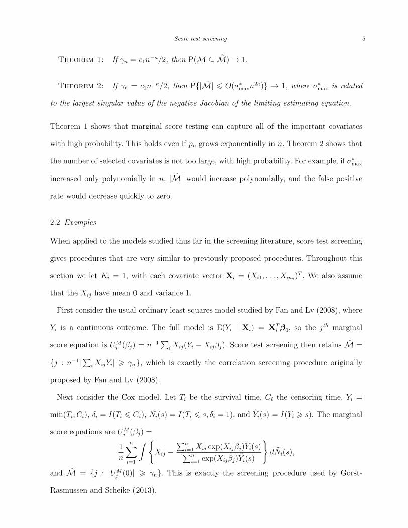
Theorem 1: If γn = c1n−κ/2, then P(M⊆ M)→ 1.
Theorem 2: If γn = c1n−κ/2, then P{|M| 6 O(σ∗maxn
2κ)} → 1, where σ∗max is related
to the largest singular value of the negative Jacobian of the limiting estimating equation.
Theorem 1 shows that marginal score testing can capture all of the important covariates
with high probability. This holds even if pn grows exponentially in n. Theorem 2 shows that
the number of selected covariates is not too large, with high probability. For example, if σ∗max
increased only polynomially in n, |M| would increase polynomially, and the false positive
rate would decrease quickly to zero.
2.2 Examples
When applied to the models studied thus far in the screening literature, score test screening
gives procedures that are very similar to previously proposed procedures. Throughout this
section we let Ki = 1, with each covariate vector Xi = (Xi1, . . . , Xipn)T . We also assume
that the Xij have mean 0 and variance 1.
First consider the usual ordinary least squares model studied by Fan and Lv (2008), where
Yi is a continuous outcome. The full model is E(Yi | Xi) = XTi β0, so the jth marginal
score equation is UMj (βj) = n−1
∑iXij(Yi −Xijβj). Score test screening then retains M =
{j : n−1|∑
iXijYi| > γn}, which is exactly the correlation screening procedure originally
proposed by Fan and Lv (2008).
Next consider the Cox model. Let Ti be the survival time, Ci the censoring time, Yi =
min(Ti, Ci), δi = I(Ti 6 Ci), Ni(s) = I(Ti 6 s, δi = 1), and Yi(s) = I(Yi > s). The marginal
score equations are UMj (βj) =
1
n
n∑i=1
∫ {Xij −
∑ni=1Xij exp(Xijβj)Yi(s)∑ni=1 exp(Xijβj)Yi(s)
}dNi(s),
and M = {j : |UMj (0)| > γn}. This is exactly the screening procedure used by Gorst-
Rasmussen and Scheike (2013).

6 Biometrics, December 2008
Finally consider a nonparametric model, where we assume only that P(Yi < y | Xi) has
a continuous distribution function F0(y;Xi,β0) whose dependence on Xi is parametrized
by β0. Conditional on Xl and Xm, F0(Yl;Xl,β0) and F0(Ym;Xm,β0) are independent and
identically distributed uniform random variables. This motivates defining U(β) =
1
n2
n∑m=1
n∑l=1
Xl
[I{F0(Yl;Xl,β) < F0(Ym;Xm,β)} − 1
2
].
Since E{U(β0)} = 0, this is an unbiased estimating equation for β0. Though it cannot
be used to estimate β0 because the functional form of F0 is unknown, it is still useful for
constructing a screening procedure. The marginal score equations are UMj (βj) =
1
n2
n∑m=1
n∑l=1
Xlj
[I{F0(Yl;Xlj, βj) < F0(Ym;Xmj, βj)} −
1
2
].
When βj = 0, F0(y;Xlj, 0) is a monotone function that does not depend on Xlj, which implies
that UMj (0) = n−2
∑lmXlj{I(Yl < Ym) − 1/2} and therefore M = {j : |n−2
∑lmXljI(Yl <
Ym)| > γn}. This is very similar to proposal of Zhu et al. (2011), who suggested M = [j :
n−1∑
m{n−1∑
lXljI(Yl < Ym)}2 > γn].
Each of these screening procedures can be implemented as or more quickly than the corre-
sponding Wald screening. In addition, the nonparametric screening procedure is impossible
in the Wald framework. Each of these screening procedures can be theoretically justified by
verifying Condition 1 and applying Theorems 1 and 2.
3. Reproducible screening threshold
In practice, it is unclear how best to choose the screening threshold γn. Fan and Lv (2008)
suggested retaining the top n/ log n covariates. Zhao and Li (2012) proposed a method to
choose γn based on the desired false positive rate of the set of retained covariates. Similarly,
Zhu et al. (2011) suggested simulating auxiliary variables and setting the threshold so that no
auxiliary variables are retained, and proved that this procedure controls the false positive rate
of screening. Finally, He and Lin (2011) used the stability selection approach of Meinshausen

Score test screening 7
and Buhlmann (2010) to retain covariates that are frequently selected when screening is
performed on multiple subsamples of the data.
Though controlling the false positive rate is important, we believe that in practice the
more relevant issue is the reproducibility of the screening procedure. Let M(j) be the top j
variables retained after screening our observed data. Suppose we had B other independent
samples of the same size, from the same generating distribution, and let M(j)b be the top j
variables we retain after screening the bth sample. Finally, let O(j)b = |M(j)
b ∩M(j)| be the size
of the overlap between the two sets. We would like to choose j such that the O(j)b are large
on average, so that our screening results are reproducible across different samples. On the
other hand, when j is large, the O(j)b will be large even if no variables were truly associated
with the outcome, so reproducibility would be uninformative.
We propose comparing the size of the overlap to the number we would expect by chance
under the null hypothesis that none of the pn variables are associated with the outcome. The
variables in M(j)b can then be thought of as having been chosen at random. Conditional on
the observed dataset, the O(j)b would therefore follow a hypergeometric distribution, with
EH0(O(j)b ) =
j2
p, varH0(O
(j)b ) =
j2(p− j)2
p2(p− 1),
where the subscripts indicate that the expectation and variance are calculated under H0. We
propose to retain the top j variables such that the average of the O(j)b shows the greatest
deviation from EH0(O(j)b ), standardized by varH0(O
(j)b ).
Because we do not have B independent datasets, we approximate the M(j)b using boot-
strap samples of our observed data. Specifically, our threshold for reproducible screening is
calculated as follows:
(1) Choose a step size s and let J = {is : i ∈ N, 1 6 is 6 pn}.
(2) For each j ∈ J , screen the observed data to obtain M(j).
(3) For each j ∈ J , generate B bootstrap samples and screen the bth sample to get M(j)b .

8 Biometrics, December 2008
(4) Let O(j)b = |M(j)
b ∩ M(j)|.
(5) Retain M(j∗), where
j∗ = arg maxj∈J
B−1∑
bO(j)b − EH0(O
(j)b )
{B−1varH0(O(j)b )}−1/2
.
When the step size s = 1, we search for the optimal j across all j = {1, . . . , pn}. In practice,
to reduce computation time we can search over a smaller subset by taking a larger step size.
Our method is closely related to higher criticism thresholding (Donoho and Jin, 2008).
There, the authors also consider the null hypothesis that none of the pn variables are
associated with the outcome. They further assume that the variables are independent. Under
this null the p-values of association are independent uniform random variables, so the jth-
most significant p-value should approximately behave like a normal random variable with
mean j/pn and variance j/pn(1−j/pn). Higher criticism thresholding finds the j ∈ {1, . . . , pn}
such that the jth-most significant observed p-value shows the greatest deviation from j/pn,
standardized by the variance. It then retains the top j variables. Higher criticism thresholding
thus focuses on the significance levels of individual variables, while our procedure evaluates
the reproducibility of entire sets of retained covariates.
4. Iterative score test screening
When the covariates are highly correlated, marginal screening may incur a large number
of false positives, and may miss covariates that are only important conditional on other
covariates. Fan and Lv (2008) and Fan et al. (2009) therefore proposed iterative screening:
an initial set of covariates is first identified using marginal screening. Next a multivariate
regularized selection procedure is used to further select a subset of these covariates. Finally
the remaining covariates are again screened individually, but this time controlling for the
covariates in the subset. All selected covariates are subjected to multivariate selection again,
and the procedure iterates until some stopping rule is achieved.

Score test screening 9
However, this algorithm requires fitting regularized regression estimates at each step,
which for complicated models can be difficult to implement and computationally intensive.
Furthermore, its theoretical properties are very difficult to analyze. Zhu et al. (2011) proposed
an alternative method which at each step performs marginal screening on the projections
of each remaining covariate onto the orthogonal complement of the columns space of the
already selected covariates. This method is akin to forward selection, so a covariate cannot
be dropped from the selected set once it has been added.
Our score-test screening perspective suggests a new approach to iterative screening:
(1) Set β(0) = 0.
(2) For k = 1, . . . , K:
(a) Let b(k) = β(k−1) − αkU(β(k−1)) for some step size αk.
(b) Let β(k) = ΠR(b(k)), where ΠR : Rpn → Rpn is the Euclidean projection onto the
`1-ball of radius R.
(3) Retain covariates M = {j : β(K)j 6= 0}, where β
(k)j is the jth component of β(k).
The intuition is that when k = 1, step 2(a) is equivalent to calculating the marginal score
statistics UMj (0) and step 2(b) sets all but the largest of them to zero. Thus after a single
iteration, this procedure is identical to score test screening. When k > 1, step 2(a) controls
for the covariates selected in β(k−1) by using −αkU(β(k−1)) to update the importance of the
covariate. Step 2(b) then again selects only the top covariates. In the ideal case where the
sample size is infinite and β(k−1) = β0, step 2(a) gives b(k) = β0 and step 2(b) selects the
largest components of β0.
Our algorithm has several advantages. First, it does not require fitting any regularized
regression estimates and is relatively computationally convenient. The evaluations of the
U(β(k−1) are quick to compute, and a simple algorithm for implementing the projection
ΠR can be found in Daubechies et al. (2008), with a more efficient procedure proposed by

10 Biometrics, December 2008
Duchi et al. (2008). Second, covariates can be dropped from the retained set as the iteration
progresses, which is an improvement over forward selection. Third, our algorithm exactly
corresponds to projected subgradient methods for minimizing nonsmooth functions. In fact,
if U(β) is the subdifferential of some loss function f(β), it has been shown that
limk→∞
f(β(k)) = inf‖β‖16R
f(β)
for certain choices of αk (Shor et al., 1985). The minimization problem on the right-hand
side is exactly equivalent to the lasso (Tibshirani, 1996) with loss function f , and this links
our iterative screening algorithm to sparse regression methods. Finally, when f is smooth,
Agarwal et al. (2012) proved that β(k) converges to β0 under certain conditions, and if a
similar result holds for nonsmooth f , this connection may allow for a theoretical analysis of
iterative score test screening.
There are three tuning parameters we must set when implementing iterative screening:
the radius R, the step sizes αk, and the maximum number of iterations. We can choose
R by either guessing the `1-norm of the true β0. Since our algorithm can be viewed as a
regression estimator, we can also minimize information criteria or cross-validated prediction
errors. Since iterative screening tends to be time-consuming in high-dimensions, it is easiest
to avoid cross-validation and to use a liberal guess for ‖β0‖1. To set the step sizes, one
popular rule is to let the αk be square summable but not summable, with αk = γ/k. To
choose γ, we first note that it can be shown that
mink=1,...,K
f(β(k))− inf‖β‖16R
f(β) 6D2 +G2
∑Kk=1 α
2k
2∑K
k=1 αk,
where D is the Euclidean distance from β(0) to a point that minimizes f and G is an
upper bound on U(β(k)) for all k (Shor et al., 1985). When αk = γ/k, this converges to
zero as K → ∞, but fixing K we can derive that the right-hand side is minimized at
γ2 = D2(G2∑K
k=1 α2k)−1 → D2(G2π2/6)−1. We propose approximating D by R and G by
‖U(β(0))‖2 to get step sizes αk = R√
6/{kπ‖U(0)‖2}. Finally, the maximum number of

Score test screening 11
iterations should ideally be as large as possible, with the speed of convergence depending
on the restricted convexity and smoothness of f (Agarwal et al., 2012). In practice we stop
after either U(β(k)) ≈ 0, β(k−1) ≈ β(k), or K = 250 iterations. Early stopping can be viewed
as another way of regularizing the regression estimate β.
5. Simulations
5.1 Settings
We illustrate our marginal and iterative score test screening on data simulated from four
models, described below along with their corresponding estimating equations. We ran 100
simulations, each with n = 400 observations and pn = 10, 000 covariates. We compared our
methods to the semiparametric screening of Zhu et al. (2011), and when possible we also
compared to Wald and nonparametric screening.
Example 1 (accelerated failure time model). The accelerated failure time model is a useful
alternative to the Cox model for survival outcomes (Wei, 1992) and posits that log(Ti) =
XTi β0 + εi, where Ti are the survival times, Xi are pn × 1 covariate vectors, and εi are
independent of Xi. We only observe follow-up times Yi = min(Ti, Ci) and censoring indicators
δi = I(Ti 6 Ci), but the β0 can be estimated using the estimating equation U(β) =
n−1n∑l=1
n∑m=1
(Xm −Xl)I{el(β) 6 em(β)}δi,
where ei(β) = log(Yi)−XTi β (Tsiatis, 1996; Jin et al., 2003; Cai et al., 2009).
Score test screening retains
M = {j : |∑lm
(Xmj −Xlj)I(Yl 6 Ym)δl| > γn},
and it is simple to verify Condition 1 for this procedure using Berstein’s inequality for U-
statistics (Hoeffding, 1963). We implemented Wald test screening using the estimator of
Jin et al. (2003), available in the R package lss. Nonparametric screening has not been
developed for this model.
12 Biometrics, December 2008
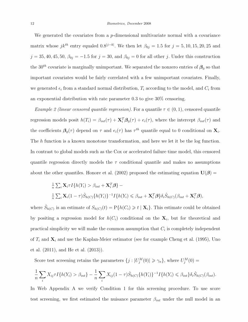
We generated the covariates from a p-dimensional multivariate normal with a covariance
matrix whose jkth entry equaled 0.8|j−k|. We then let β0j = 1.5 for j = 5, 10, 15, 20, 25 and
j = 35, 40, 45, 50, β0j = −1.5 for j = 30, and β0j = 0 for all other j. Under this construction
the 30th covariate is marginally unimportant. We separated the nonzero entries of β0 so that
important covariates would be fairly correlated with a few unimportant covariates. Finally,
we generated εi from a standard normal distribution, Ti according to the model, and Ci from
an exponential distribution with rate parameter 0.3 to give 30% censoring.
Example 2 (linear censored quantile regression). For a quantile τ ∈ (0, 1), censored quantile
regression models posit h(Ti) = βint(τ) + XTi β0(τ) + ei(τ), where the intercept βint(τ) and
the coefficients β0(τ) depend on τ and ei(τ) has τ th quantile equal to 0 conditional on Xi.
The h function is a known monotone transformation, and here we let it be the log function.
In contrast to global models such as the Cox or accelerated failure time model, this censored
quantile regression directly models the τ conditional quantile and makes no assumptions
about the other quantiles. Honore et al. (2002) proposed the estimating equation U(β) =
1n
∑iXiτI{h(Yi) > βint + XT
i β}−
1n
∑iXi(1− τ)Sh(C){h(Yi)}−1I{h(Yi) 6 βint + XT
i β}δiSh(C)(βint + XTi β),
where Sh(C) is an estimate of Sh(C)(t) = P{h(Ci) > t | Xi}. This estimate could be obtained
by positing a regression model for h(Ci) conditional on the Xi, but for theoretical and
practical simplicity we will make the common assumption that Ci is completely independent
of Ti and Xi and use the Kaplan-Meier estimator (see for example Cheng et al. (1995), Uno
et al. (2011), and He et al. (2013)).
Score test screening retains the parameters {j : |UMj (0)| > γn}, where UM
j (0) =
1
n
∑i
XijτI{h(Yi) > βint} −1
n
∑i
Xij(1− τ)Sh(C){h(Yi)}−1I{h(Yi) 6 βint}δiSh(C)(βint).
In Web Appendix A we verify Condition 1 for this screening procedure. To use score
test screening, we first estimated the nuisance parameter βint under the null model in an
Score test screening 13
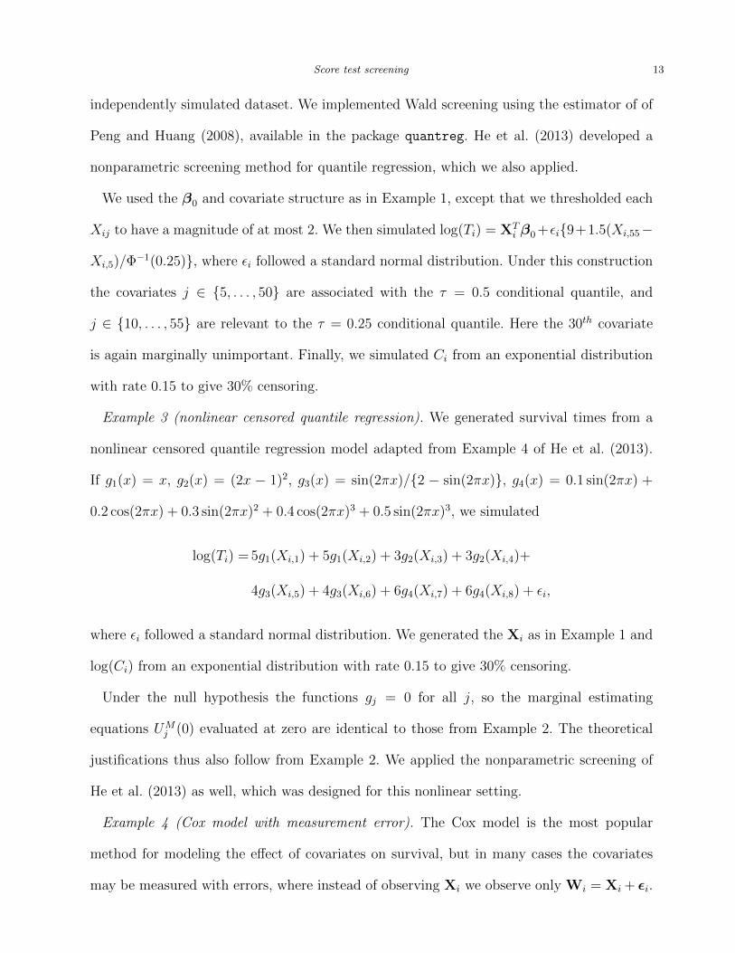
independently simulated dataset. We implemented Wald screening using the estimator of of
Peng and Huang (2008), available in the package quantreg. He et al. (2013) developed a
nonparametric screening method for quantile regression, which we also applied.
We used the β0 and covariate structure as in Example 1, except that we thresholded each
Xij to have a magnitude of at most 2. We then simulated log(Ti) = XTi β0+εi{9+1.5(Xi,55−
Xi,5)/Φ−1(0.25)}, where εi followed a standard normal distribution. Under this construction
the covariates j ∈ {5, . . . , 50} are associated with the τ = 0.5 conditional quantile, and
j ∈ {10, . . . , 55} are relevant to the τ = 0.25 conditional quantile. Here the 30th covariate
is again marginally unimportant. Finally, we simulated Ci from an exponential distribution
with rate 0.15 to give 30% censoring.
Example 3 (nonlinear censored quantile regression). We generated survival times from a
nonlinear censored quantile regression model adapted from Example 4 of He et al. (2013).
If g1(x) = x, g2(x) = (2x − 1)2, g3(x) = sin(2πx)/{2 − sin(2πx)}, g4(x) = 0.1 sin(2πx) +
0.2 cos(2πx) + 0.3 sin(2πx)2 + 0.4 cos(2πx)3 + 0.5 sin(2πx)3, we simulated
log(Ti) = 5g1(Xi,1) + 5g1(Xi,2) + 3g2(Xi,3) + 3g2(Xi,4)+
4g3(Xi,5) + 4g3(Xi,6) + 6g4(Xi,7) + 6g4(Xi,8) + εi,
where εi followed a standard normal distribution. We generated the Xi as in Example 1 and
log(Ci) from an exponential distribution with rate 0.15 to give 30% censoring.
Under the null hypothesis the functions gj = 0 for all j, so the marginal estimating
equations UMj (0) evaluated at zero are identical to those from Example 2. The theoretical
justifications thus also follow from Example 2. We applied the nonparametric screening of
He et al. (2013) as well, which was designed for this nonlinear setting.
Example 4 (Cox model with measurement error). The Cox model is the most popular
method for modeling the effect of covariates on survival, but in many cases the covariates
may be measured with errors, where instead of observing Xi we observe only Wi = Xi + εi.

14 Biometrics, December 2008
Not accounting for measurement error can result in bias, and to address this issue Song and
Huang (2005) proposed the corrected score equation U(β) =
1
n
n∑i=1
∫ [Wi +D(β)−
∑ni=1 Wi(β, s) exp{Wi(β, s)
Tβ}Yi(s)∑ni=1 exp{Wi(β, s)Tβ}Yi(s)
]dNi(s),
where Wi(β, s) = Wi+D(β)dNi(s), D(β) = E{εi exp(εTi β)}/E{exp(εTi β)}−E(εi), Ni(s) =
I(Ti 6 s, δi = 1) is the observed failure process, and Yi(s) = I(Yi > s) is the at-risk process.
The D(β) term is unknown in general unless the distribution of εi is known.
Under the null hypothesis of β0 = 0, D(0) = 0, so score test screening retains
M =
[j :
∣∣∣∣∣ 1nn∑i=1
∫ {Wij −
∑ni=1WijYi(s)∑ni=1 Yi(s)
}dNi(s)
∣∣∣∣∣ > γn
]regardless of the distribution of εi. Condition 1 can be verified using Lemmas 2 and 3 of
Gorst-Rasmussen and Scheike (2013). Wald screening is not possible without knowing the
distribution of εi, and nonparametric screening has not been developed for this model.
We generated the covariates and set β0 as in Example 1. We then generated the Ti from the
usual Cox model with baseline hazard function equal to 1. Next we let Wi = Xi + εi, where
the εi were independent of the Xi and normally distributed with a compound symmetry
covariance matrix with correlation parameter 0.5. We generated log(Ci) from an exponential
distribution with rate parameter 0.3 to give 30% censoring.
5.2 Results
[Table 1 about here.]
These simulations were run on machines with 2 GHz Intel Xeon cores with 4GB of memory
per core. Table 1 reports the average runtimes of these various screening methods and
shows that our marginal score test procedure is by far the most computationally efficient. In
Example 1 it is many orders of magnitude faster than Wald screening, and in Examples 2 and
3 it is 60 times faster than the nonparametric method of He et al. (2013). In each example
it is also at least twice as fast as the semiparametric estimator of Zhu et al. (2011).
Score test screening 15
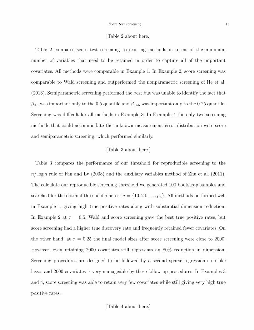
[Table 2 about here.]
Table 2 compares score test screening to existing methods in terms of the minimum
number of variables that need to be retained in order to capture all of the important
covariates. All methods were comparable in Example 1. In Example 2, score screening was
comparable to Wald screening and outperformed the nonparametric screening of He et al.
(2013). Semiparametric screening performed the best but was unable to identify the fact that
β0,5 was important only to the 0.5 quantile and β0,55 was important only to the 0.25 quantile.
Screening was difficult for all methods in Example 3. In Example 4 the only two screening
methods that could accommodate the unknown measurement error distribution were score
and semiparametric screening, which performed similarly.
[Table 3 about here.]
Table 3 compares the performance of our threshold for reproducible screening to the
n/ log n rule of Fan and Lv (2008) and the auxiliary variables method of Zhu et al. (2011).
The calculate our reproducible screening threshold we generated 100 bootstrap samples and
searched for the optimal threshold j across j = {10, 20, . . . , pn}. All methods performed well
in Example 1, giving high true positive rates along with substantial dimension reduction.
In Example 2 at τ = 0.5, Wald and score screening gave the best true positive rates, but
score screening had a higher true discovery rate and frequently retained fewer covariates. On
the other hand, at τ = 0.25 the final model sizes after score screening were close to 2000.
However, even retaining 2000 covariates still represents an 80% reduction in dimension.
Screening procedures are designed to be followed by a second sparse regression step like
lasso, and 2000 covariates is very manageable by these follow-up procedures. In Examples 3
and 4, score screening was able to retain very few covariates while still giving very high true
positive rates.
[Table 4 about here.]
16 Biometrics, December 2008
Table 4 reports the performance of our iterative screening procedure from Section 4, which
we applied to the parametric models in Examples 1 and 2 with R = 20. In those models the
30th covariate had a nonzero coefficient in the true model but was marginally unassociated
with the outcome. In Example 1 iterative screening was able to capture that covariate in
nearly all of the simulations. In Example 2, iterative screening was still to capture the variable
after retaining only around 200-300 variables, as opposed to marginal score screening, which
had to retain thousands of variables. However, the hidden covariate was only captured in
very few simulations, indicating that variable screening for Example 2 is a difficult problem.
6. Data analysis
6.1 Analysis methods
We were interested in identifying genes highly associated with the 10% conditional quantile
of the survival distribution of MM patients, because these genes are likely to important
in high-risk MM. Previous studies have searched for genes associated with patient survival
(Shaughnessy et al., 2007; Decaux et al., 2008), but their analyses did not recognize that
some genes may only affect certain quantiles of the conditional survival distribution.
We used gene expression and survival outcome data from newly diagnosed multiple myeloma
patients who were recruited into clinical trials UARK 98-026 and UARK 2003-33, which stud-
ied the total therapy II (TT2) and total therapy III (TT3) treatment regimes, respectively.
These data are described in Zhan et al. (2006) and Shaughnessy et al. (2007), and can be
obtained through the MicroArray Quality Control Consortium II study (Shi et al., 2010),
available on GEO (GSE24080). Gene expression profiling was performed using Affymetrix
U133Plus2.0 microarrays, and we averaged the expression levels of probesets corresponding
to the same gene, resulting in 33,326 covariates. We used the TT2 arm as a training set,
giving us 340 subjects and 126 observed deaths, we validated the results on the TT3 arm.

Score test screening 17
To identify these high-risk genes we used the censored quantile regression of Honore et al.
(2002), described earlier in Example 2 in Section 5.1, with the transformation function
h = log. First, in the screening step we compared Wald screening with the estimator of
Peng and Huang (2008), marginal score screening, the semiparametric method of Zhu et al.
(2011), the nonparametric method of He et al. (2013), and iterative score screening. In the
score screening procedures we estimated the nuisance intercept parameter from another MM
dataset collected by Avet-Loiseau et al. (2009). For iterative score screening we set R = 20.
Second, to set a screening threshold we retained the top n/ log n covariates from Wald and
nonparametric screening, used our reproducible screening threshold for score screening, and
used the auxiliary variables procedure of Zhu et al. (2011) for semiparametric screening. For
reproducible screening we generated 100 bootstrap samples and searched for the optimal
threshold j across j = {10, 20, . . . , pn}, as in the simulations.
Finally, we used the screened covariates to estimate regression models. To our knowledge
there do not exist any computationally convenient procedures for censored quantile regression
for arbitrary quantiles that can be computed in high-dimensions, so we used our projected
subgradient method from Section 4 to serve as a regression estimator. We tuned the procedure
by selecting the value of R that minimized an approximate Bayesian Information Criterion,
which we calculated as ‖nU(βR)‖22 + ‖βR‖0 log n with U the estimating equation of Honore
et al. (2002) and βR the regression estimate for a given value of R.
6.2 Results
Wald screening required 930 seconds, the nonparametric screening of He et al. (2013) required
240 seconds, iterative score screening required 84 seconds, the semiparametric screening of
Zhu et al. (2011) required 44 seconds, and marginal score screening took only 5 seconds.
Because of the computational efficiency of score screening, calculating the reproducible
screening threshold required only 934 seconds, which was still just as fast as Wald screening.

18 Biometrics, December 2008
[Table 5 about here.]
Table 5 reports the genes selected in the final censored quantile regression models. Iter-
ative and reproducible score screening behaved very similarly, giving nearly identical final
models. However, they shared no genes in common with the results of the other screening
methods. One possible reason is that the correlations between the selected genes were not
low. For example, among the top 100 genes selected by Wald screening, 20% of the pairwise
correlations were above 0.25 and the largest reached 0.73, and for score screening 20% of
the correlations were at least 0.58 and reached 0.99. In other words, the different screening
methods most likely selected blocks of correlated covariates together, and the same covariates
could be ranked very differently by different methods if they were in different blocks. This
highlights the importance of reproducibility.
To choose between the four models, we used the fitted regression models to predict the 0.1
conditional quantiles in the TT3 arm and calculated validation metrics in two ways. First,
to estimate the quantile prediction error we used the loss function
n−1∑i
δi
Sh(C){h(Yi)}{τ − I(Yi − Yi < 0)}Yi, (1)
where δi is the censoring indicator, Yi is the observed follow-up time, τ = 0.1 is the target
quantile, and Yi is the predicted τ conditional quantile. A similar loss function was described
by Honore et al. (2002). Second, we used the censored quantile regression approach of Peng
and Huang (2008) to estimate the associations between the predicted quantiles and the
true 0.1 quantile. We report the t-statistics of association. Table 5 shows that the models
selected after score screening performed the best under both validation metrics, followed by
semiparametric screening. In contrast, the quantiles predicted after Wald and semiparametric
screening were actually negatively associated with the true quantile. This suggests that the
true relationship between the genes and the quantile may be significantly nonlinear. This
nonlinearity can still be detected by the score screening methods.

Score test screening 19
7. Discussion
Motivated by our analysis of genomic factors influencing the high risk multiple myeloma
patients, we introduced a new framework for variable screening based on score tests. Score
screening is widely applicable to parametric, semiparametric, and nonparametric models,
relatively easy to theoretically justify, and computationally efficient. Using score test screen-
ing in our MM analysis resulted in a predictive model for the conditional 10% quantile (high
risk group) which was more accurate the models obtained using other screening methods.
We introduced a method for selecting the number of covariates to retain based on the
principle of reproducible screening. It would be interesting to investigate the sure screening
and false positive control properties of this procedure, in the context of Theorems 1 and
2. Our score testing framework also suggested a new approach to iterative screening based
on projected subgradient methods, which can be applied even to nonsmooth estimating
equations. It is related to sparse regression techniques and it is possible that this connection
can lead to better a theoretical understanding of iterative screening, which is still elusive.
8. Supplementary Materials
Web Appendix A, which contains the theoretical justification of score screening and is
referenced in Section 2, is available with this paper at the Biometrics website on Wiley
Online Library. We also provide a zip file including an R implementation of our screening
methods, a simulation example, and instructions.
Acknowledgments
We are grateful to the editor, the associate editor, and the anonymous referee for their helpful
comments. We also thank Professors Lee Dicker and Julian Wolfson for reading an earlier
version of this manuscript. This research is partially supported by an NIH grant.

20 Biometrics, December 2008
References
Agarwal, A., Negahban, S., and Wainwright, M. J. (2012). Fast global convergence of gradient
methods for high-dimensional statistical recovery. The Annals of Statistics 40, 2452–
2482.
Avet-Loiseau, H., Li, C., Magrangeas, F., Gouraud, W., Charbonnel, C., Harousseau, J.-L.,
Attal, M., Marit, G., Mathiot, C., Facon, T., et al. (2009). Prognostic significance of
copy-number alterations in multiple myeloma. Journal of Clinical Oncology 27, 4585–
4590.
Buhlmann, P. L., van de Geer, S. A., and Van de Geer, S. (2011). Statistics for high-
dimensional data. Springer.
Cai, T., Huang, J., and Tian, L. (2009). Regularized estimation for the accelerated failure
time model. Biometrics 65, 394–404.
Cheng, S., Wei, L., and Ying, Z. (1995). Analysis of transformation models with censored
data. Biometrika 82, 835–845.
Daubechies, I., Fornasier, M., and Loris, I. (2008). Accelerated projected gradient method
for linear inverse problems with sparsity constraints. Journal of Fourier Analysis and
Applications 14, 764–792.
Decaux, O., Lode, L., Magrangeas, F., Charbonnel, C., Gouraud, W., Jezequel, P., Attal,
M., Harousseau, J. L., Moreau, P., Bataille, R., Campion, L., Avet-Loiseau, H., and
Minvielle, S. (2008). Prediction of survival in multiple myeloma based on gene expression
profiles reveals cell cycle and chromosome instability signatures in high-risk patients and
hyperdiploid signatures in low-risk patients: a study of the Intergroupe Francophone du
Myelome. Journal of Clinical Oncology 26, 4798–4805.
Donoho, D. and Jin, J. (2008). Higher criticism thresholding: Optimal feature selection when
useful features are rare and weak. Proceedings of the National Academy of Sciences 105,

Score test screening 21
14790–14795.
Duchi, J., Shalev-Shwartz, S., Singer, Y., and Chandra, T. (2008). Efficient projections
onto the `1-ball for learning in high dimensions. In Proceedings of the 25th international
conference on Machine learning, pages 272–279. ACM.
Fan, J., Feng, Y., and Song, R. (2011). Nonparametric independence screening in sparse
ultra-high-dimensional additive models. Journal of the American Statistical Association
106, 544–557.
Fan, J. and Lv, J. (2008). Sure independence screening for ultrahigh dimensional feature
space. Journal of the Royal Statistical Society, Ser. B 70, 849–911.
Fan, J., Samworth, R., and Wu, Y. (2009). Ultrahigh dimensional feature selection: beyond
the linear model. The Journal of Machine Learning Research 10, 2013–2038.
Fan, J. and Song, R. (2010). Sure independence screening in generalized linear models and
NP-dimensionality. The Annals of Statistics 38, 3567–3604.
Gorst-Rasmussen, A. and Scheike, T. H. (2013). Independent screening for single-index
hazard rate models with ultra-high dimensional features. Journal of the Royal Statistical
Society, Ser. B 75, 217–245.
He, Q. and Lin, D.-Y. (2011). A variable selection method for genome-wide association
studies. Bioinformatics 27, 1–8.
He, X., Wang, L., and Hong, H. G. (2013). Quantile-adaptive model-free variable screening
for high-dimensional heterogeneous data. The Annals of Statistics 41, 342–369.
Hoeffding, W. (1963). Probability inequalities for sums of bounded random variables. Journal
of the American Statistical Association 58, 13–30.
Honore, B., Khan, S., and Powell, J. L. (2002). Quantile regression under random censoring.
Journal of Econometrics 109, 67–105.
Jin, Z., Lin, D. Y., Wei, L. J., and Ying, Z. (2003). Rank-based inference for the accelerated
22 Biometrics, December 2008
failure time model. Biometrika 90, 341–353.
Li, G., Peng, H., Zhang, J., and Zhu, L. (2012). Robust rank correlation based screening.
The Annals of Statistics 40, 1846–1877.
Li, R., Zhong, W., and Zhu, L. (2012). Feature screening via distance correlation learning.
Journal of the American Statistical Association 107, 1129–1139.
Meinshausen, N. and Buhlmann, P. (2010). Stability selection. Journal of the Royal
Statistical Society: Series B (Statistical Methodology) 72, 417–473.
Peng, L. and Huang, Y. (2008). Survival analysis with quantile regression models. Journal
of the American Statistical Association 103, 637–649.
Portnoy, S. (2003). Censored regression quantiles. Journal of the American Statistical
Association 98, 1001–1012.
Shaughnessy, J., Zhan, F., Burington, B. E., Huang, Y., Colla, S., Hanamura, I., Stewart,
J. P., Kordsmeier, B., Randolph, C., Williams, D. R., et al. (2007). A validated gene
expression model of high-risk multiple myeloma is defined by deregulated expression of
genes mapping to chromosome 1. Blood 109, 2276–2284.
Shi, L., Campbell, G., Jones, W. D., et al. (2010). The MAQC-II Project: A comprehensive
study of common practices for the development and validation of microarray-based
predictive models. Nature Biotechnology 28, 827–838.
Shor, N. Z., Kiwiel, K. C., and Ruszcayski, A. (1985). Minimization methods for non-
differentiable functions. Springer-Verlag New York, Inc.
Song, X. and Huang, Y. (2005). On corrected score approach for proportional hazards model
with covariate measurement error. Biometrics pages 702–714.
Tibshirani, R. J. (1996). Regression shrinkage and selection via the lasso. Journal of the
Royal Statistical Society, Ser. B 58, 267–288.
Tsiatis, A. A. (1996). Estimating regression parameters using linear rank tests for censored
Score test screening 23
data. The Annals of Statistics 18, 354–372.
Uno, H., Cai, T., Pencina, M. J., D’Agostino, R. B., and Wei, L. J. (2011). On the C-statistics
for evaluating overall adequacy of risk prediction procedures with censored survival data.
Statistics in Medicine 30, 1105–1117.
Wang, H. J. and Wang, L. (2009). Locally weighted censored quantile regression. Journal
of the American Statistical Association 104, 1117–1128.
Wei, L. J. (1992). The accelerated failure time model: a useful alternative to the cox regression
model in survival analysis. Statistics in Medicine 11, 1871–1879.
Zhan, F., Huang, Y., Colla, S., Stewart, J., Hanamura, I., Gupta, S., Epstein, J., Yaccoby,
S., Sawyer, J., Burington, B., et al. (2006). The molecular classification of multiple
myeloma. Blood 108, 2020.
Zhao, S. D. and Li, Y. (2012). Principled sure independence screening for Cox models with
ultra-high-dimensional covariates. Journal of Multivariate Analysis 105, 397–411.
Zhu, L.-P., Li, L., Li, R., and Zhu, L.-X. (2011). Model-free feature screening for ultrahigh-
dimensional data. Journal of the American Statistical Association 106, 1464–1475.
Received October 2007. Revised February 2008. Accepted March 2008.

24 Biometrics, December 2008
Table 1Average runtime (seconds) of different screening methods.
Example Wald Score Zhu et al. (2011) He et al. (2013)
1 16533.06 1.91 8.202 1206.89 2.42 7.16 123.273 0.21 0.88 5.414 2.19 5.76

Score test screening 25
Table 2Medians (interquartile ranges) of minimum model sizes required to retain the covariates in the second column. In
Example 2, β0,5 is relevant only when τ = 0.5 and β0,55 is relevant only when τ = 0.25. Similarly, in Example 3 β0,5is relevant only when τ = 0.5 and β0,25 is relevant only when τ = 0.25.
Covariates Wald Score Zhu et al. (2011) He et al. (2013)
Example 1All 5699.5 (4231) 5500 (4091) 5645 (5022.25)
Example 2, τ = 0.5All 6070.5 (4655.75) 6168.5 (3832.5) 5742 (4609.25) 9166 (2057)β0,5 30.5 (62.75) 36.5 (94.25) 23 (28.25) 3451 (5856.5)β0,55 2393 (4184.5) 1882.5 (5565.75) 547.5 (1028.25) 3708.5 (5094.5)
Example 2, τ = 0.25All 5111 (4736.5) 5094 (4104.5) 5742 (4376) 9720 (554)β0,5 1724.5 (4758.25) 1763 (5112.75) 23 (28.25) 5516.5 (5380.5)β0,55 67.5 (309) 88.5 (273.5) 547.5 (1028.25) 2381 (6252.5)
Example 3, τ = 0.5All 9620 (548.25) 9729 (337.75) 9277.5 (361.75) 9945 (243)
Example 4All 5495.5 (4365.5) 5584.5 (4367.5) 5483 (4237.25)

26 Biometrics, December 2008
Table 3Performance of different methods for choosing the screening threshold. Methods: RS = reproducible screening,
described in Section 3; Auxiliary = auxiliary variables method of Zhu et al. (2011). Average performance metrics(standard deviation): TP = true positive rate, TD = true discovery rate. Median size is reported (interquartile
range).
Screening Threshold TP TD Size
Example 1Wald n/ log n 90 (0) 13.64 (0) 66 (0)Score RS 86.2 (7.49) 22.84 (1.52) 40 (0)Zhu et al. (2011) Auxiliary 89.4 (2.39) 21.02 (1.46) 43 (4)
Example 2, τ = 0.5Wald n/ log n 68.9 (13.25) 10.44 (2.01) 66 (0)Score RS 62.9 (27.35) 13.26 (13) 30 (1602.5)Zhu et al. (2011) Auxiliary 40.7 (17.25) 31.18 (15.09) 15 (10.25)He et al. (2013) n/ log n 3.9 (5.84) 0.59 (0.89) 66 (0)
Example 2, τ = 0.25Wald n/ log n 62.8 (12.56) 9.52 (1.9) 66 (0)Score RS 72 (25.74) 7.73 (12.06) 1540 (1642.5)Zhu et al. (2011) Auxiliary 36.9 (15.87) 28.66 (15.87) 15 (10.25)He et al. (2013) n/ log n 5.5 (8.57) 0.83 (1.3) 66 (0)
Example 3, τ = 0.5Score RS 62.38 (15.02) 29.76 (22.56) 10 (130)Zhu et al. (2011) Auxiliary 16.38 (17.65) 49.49 (44.36) 2 (2)He et al. (2013) n/ log n 56.25 (22.86) 6.82 (2.77) 66 (0)
Example 4Score RS 68 (15.04) 26.26 (6.76) 30 (10)Zhu et al. (2011) Auxiliary 72.4 (14.36) 25.15 (4.23) 30.5 (12)

Score test screening 27
Table 4Performance of iterative screening. The second column reports the average percentage of times (SD) the marginallyunimportant variables (see Section 5.1) were capture by iterative screening. Average performance metrics (standard
deviation): TP = true positive rate, TD = true discovery rate. Median size is reported (interquartile range).
Hidden TP TD Size
Example 191 (28.76) 95.9 (6.21) 1.66 (0.42) 652 (259.5)
Example 2, τ = 0.51 (10) 79.8 (11.97) 2.71 (0.73) 282 (44.25)
Example 2, τ = 0.251 (10) 71.7 (10.83) 3.29 (0.93) 210 (64.5)

28 Biometrics, December 2008
Table 5Final regression models for the 0.1 conditional quantile of MM patient survival. Validation metrics: PE = predictionerror (1); t-statistic = t-statistic of the regression of the true 0.1 quantile on the predicted quantile, using Peng and
Huang (2008).
Validation Wald Zhu et al. (2011) He et al. (2013) Iterative Score
CDK13 ADAR ATP6 hnRNPK hnRNPKMAPKAP1 ATP6V0E1 CARD8 hnRNPKP4 hnRNPK4PEX11B DPY30 CTCF MATR3 MATR3VCP HNRNPU DDX3X OAZ1 OAZ1
NOLC1 RAB10 RAP10RPS3A RPS3ASPCS1 SPCS1SPCS2 SPCS2SUMO2 SUMO2TMBIM4 TMBIM4UBC UBC
SERP1PE 0.660 1.158 0.430 0.079 0.083
t-statistic -1.133 -0.515 1.319 1.690 1.731