score-driven models for forecasting - blasques f., koopman s.j., lucas a.. june, 14 2014

Score-driven models for forecasting

F. Blasques S.J. Koopman A. Lucas

VU University Amsterdam, Tinbergen Institute, CREATES

Eighth ECB Workshop on Forecasting Techniques

ECB, Frankfurt am Mainz, 13-14 June 2014

1 / 25 Blasques, Koopman and Lucas Score-driven models for forecasting

The basic framework

We have an observed time series y1, . . . , yn, collected in y, and

an unobserved path of equal length f1, . . . , fn, collected in f .

Assume that

DGP is y ∼ p(y;f) where f represents a time-varying

feature of the "true" model density.

time series econometrician opts for a predictive model

p̃(yt|y1, . . . , yt−1;θ), with parameter vector θ, and correctly

considers the e�ect associated with f to be time-varying.


The basic framework

Assume that

DGP is y ∼ p(y;f)

econometric model p̃(yt|y1, . . . , yt−1;θ) correctly considers

the e�ect associated with f to be time-varying.

In an observation-driven model, the time-varying e�ect is

extracted as a direct function of past data:

f̃t = f̃t(y1, . . . , yt−1;θ). We have p̃(yt|f̃t, y1, . . . , yt−1;θ).

Consider GARCH model where f is the time-varying variance,

then we have p̃(yt|f̃t;θ) ≡ N(0, f̃t) and

f̃t+1 = ω + βf̃t + α(y2t − f̃t),

and with θ = (ω, α, β)′.


The basic framework

In a general setting (Creal, Koopman & Lucas 2008, 2011, 2013),

p̃(yt|f̃t, y1, . . . , yt−1;θ) 6= N(0, f̃t),

we propose for f̃t to adopt the updating scheme

f̃t+1 = ω + βf̃t + αst,

where st is the scaled score function st = St∇t with

∇t =∂ ln p(yt|y1, . . . , yt−1, f̃t;θ)

∂f̃t,


Score-driven models

For this updating equation

f̃t+1 = ω + βf̃t + αst,

we can view updating as a steepest ascent or Newton step

for f̃t using the log conditional density

p̃(yt|f̃t, y1, . . . , yt−1;θ) as criterion function;

choice for St may be square root matrix of the inverse

Fisher information matrix;

this St accounts for curvature of density as function of f̃t;

also, under correct model speci�cation, st has unit variance.


Generalized Autoregressive Score (GAS)

The general GAS framework is

p̃(yt|f̃t, y1, . . . , yt−1;θ),

where for f̃t we adopt the updating scheme

f̃t+1 = ω + βf̃t + αst,

with st as the scaled score function st = St∇t and

∇t =∂ ln p(yt|y1, . . . , yt−1, f̃t; θ)

∂f̃t,

St = I−1/2t−1 = −Et−1

[∂2 ln p(yt|Yt−1, f̃t; θ)

∂f̃t∂f̃ ′t

]−1/2.


Illustration : volatility modeling

A class of volatility models is given by

yt = µ+ σ(f̃t)ut, ut ∼ pu(ut;θ),

f̃t+1 = ω + βf̃t + αst,

where:

σ() is some continuous function with positive support;

pu(ut; θ) is a standardized disturbance density;

st is scaled score ∂ log p(yt|f̃t, y1, . . . , yt−1;θ) / ∂f̃t.

Some special cases

σ(f̃t) = f̃t and pu is Gaussian : GAS ⇒ GARCH;

σ(f̃t) = exp(f̃t) and pu is Gaussian : GAS ⇒ EGARCH;

σ(f̃t) = exp(f̃t) and pu is Student's t : GAS ⇒ t-GAS.


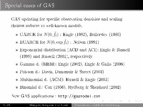
Special cases of GAS

GAS updating for speci�c observation densities and scaling

choices reduces to well-known models.

GARCH for N(0, f̃t) : Engle (1982), Bollerslev (1986)

EGARCH for N(0, exp f̃t) : Nelson (1991)

Exponential distribution (ACD and ACI): Engle & Russell

(1998) and Russell (2001), respectively

Gamma d. (MEM): Engle (2002), Engle & Gallo (2006)

Poisson d.: Davis, Dunsmuir & Street (2003)

Multinomial d. (ACM): Russell & Engle (2005)

Binomial d.: Cox (1956), Rydberg & Shephard (2002)

New GAS applications : http://gasmodel.com


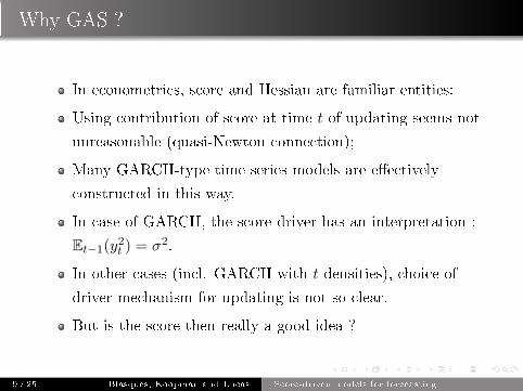
Why GAS ?

In econometrics, score and Hessian are familiar entities;

Using contribution of score at time t of updating seems not

unreasonable (quasi-Newton connection);

Many GARCH-type time series models are e�ectively

constructed in this way.

In case of GARCH, the score driver has an interpretation :

Et−1(y2t ) = σ2.

In other cases (incl. GARCH with t-densities), choice of

driver mechanism for updating is not so clear.

But is the score then really a good idea ?


Why GAS ?

On the outset:

1 GAS update is very intuitive...

2 Using the score seems optimal in some sense...

3 Likelihood and KL divergence are closely related...

Question: Is the GAS update optimal in some KL sense?

Challenge 1: GAS update is surely not always correct!

Challenge 2: Comparing di�erent observation-driven models is

only interesting under misspeci�cation with very general DGP!


DGP and Observation-Driven Model

True sequence of conditional densities:{p(yt|ft)

}, true tv parameter {ft}

Conditional densities postulated by probabilistic model:{p̃(yt|f̃t;θ

) }, �ltered tv parameter {f̃t}

p̃(yt|f̃t;θ

)is implicitly by observation equation:

yt = g(f̃t , ut ; θ

), ut ∼ pu(θ),

Observation-driven parameter update:

f̃t+1 = φ(yt , f̃t ; θ

), ∀ t ∈ N, f̃1 ∈ F ⊆ R,


Optimal Observation-Driven Update

Key objective: Characterize φ(·) that possess optimality

properties from information theoretic point of view.

Main Question: Is there an optimal form for the update

f̃t+1 = φ(yt , f̃t ; θ

), ∀ t ∈ N, f̃1 ∈ F ⊆ R,

Answer: This depends on the notion of optimality!

Result 1: Only parameter updates based on the score always

reduce the local Kullback-Leibler divergence p and p̃.

Result 2: The use of the score leads to considerably smaller

global KL divergence in empirically relevant settings.

Note: Results hold for any DGP ( any p and {ft} )


De�nitions: Local GAS Updates

GAS-update:

f̃t+1 = φ(yt , f̃t ; θ

)= ω + αs(yt, f̃t) + βf̃t, ∀ t ∈ N,

Newton-GAS update: ( ω = 0, α > 0, β = 1 )

f̃t+1 = αs(yt, f̃t) + f̃t, ∀ t ∈ N,

Local update: f̃t+1 in neighborhood of f̃t

Local optimality: Refers to local updates


De�nition II: Conditionally Expected KL Divergence

An optimal updating scheme, while subject to randomness,

should have tendency to move in correct direction:

On average, the KL divergence should reduce in expectation.

The conditionally expected KL (CKL) variation of a parameter

update from f̃t ∈ F̃ to f̃t+1 ∈ F̃ is given by

∆t−1CKL =

∫Fq(f̃t+1|f̃t, ft;θ)

[∫Yp(y|ft) ln

p̃(y|f̃t;θ)

p̃(y|f̃t+1;θ)dy

]df̃t+1,

where q(f̃t+1|f̃t, ft;θ) denotes the density of f̃t+1 conditional on

both f̃t and ft. For a given pt, an update is CKL optimal if and

only if ∆t−1CKL ≤ 0.


Propositions 1 and 2

... subject to speci�c regularity conditions

Proposition 1 :

Every Newton-GAS update (f̃t+1 = αst + f̃t) is locally RKL

optimal and CKL optimal for any true density pt.

These properties can be generalized to `score-equivalent'

updates, but we require a fundamental sign condition.

Proposition 2 :

For any given true density pt, a parameter update is locally

RKL optimal and CKL optimal if and only if the parameter

update is score-equivalent, that is

sign(∆φ(f, y;θ)) = sign(∇(f, y;θ))


Proposition 3

For the GAS updating

f̃t+1 = ω + βf̃t + αst,

we require speci�c and di�erent conditions for ω, β and α to

state

Proposition 3 :

The GAS update is locally RKL optimal and CKL optimal, for

every pt.


Example RKL for GARCH

The GAS volatility model with a normal distribution reduces to

the standard GARCH model.

Then the necessary condition is α |y2t − f̃t| > |ω + (β − 1)f̃t| :

From this condition we learn that the update becomes

convincingly more RKL optimal if the observed y2t deviates

considerably from the �ltered volatility f̃t.

Similar conditions can be stated for other densities and for CKL

optimality.


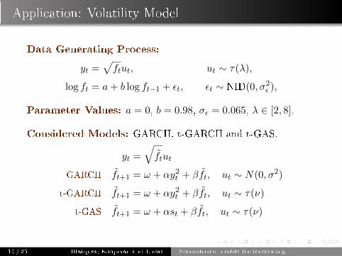
Application: Volatility Model

Data Generating Process:

yt =√ftut, ut ∼ τ(λ),

log ft = a+ b log ft−1 + εt, εt ∼ NID(0, σ2ε ),

Parameter Values: a = 0, b = 0.98, σε = 0.065, λ ∈ [2, 8].

Considered Models: GARCH, t-GARCH and t-GAS.

yt =

√f̃tut

GARCH f̃t+1 = ω + αy2t + βf̃t, ut ∼ N(0, σ2)

t-GARCH f̃t+1 = ω + αy2t + βf̃t, ut ∼ τ(ν)

t-GAS f̃t+1 = ω + αst + βf̃t, ut ∼ τ(ν)


Application: Volatility Model

Data Generating Process:

yt =√ftut, ut ∼ τ(λ),

log ft = a+ b log ft−1 + εt, εt ∼ NID(0, σ2ε ),

Parameter Values: a = 0, b = 0.98, σε = 0.065, λ ∈ [2, 8].

Note: Comparison at pseudo-true parameters θ∗ = arg minKL

Sample size T: Large enough for ML estimator to converge to

pseudo-true parameter (at 3rd decimal place).

Asymptotic Theory: Convergence of ML estimator to

pseudo-true parameter in misspeci�ed GAS, see BKL (2013).


The pseudo-true parameters

3 4 5 6 7 8 90

0.1

0.2

Pseudo-trueω

λ

3 4 5 6 7 8 90

0.05

0.1

Pseudo-trueα

λ

3 4 5 6 7 8 90.8

0.9

1

Pseudo-trueβ

λ

3 4 5 6 7 8 90

2

4

6

8

Pseudo-trueλ

λ

GARCH

GARCH−t

GAS

Figure: DGP with a = 0, b = 0.98, σε = 0.065 and λ ∈ [3, 8]. Each

model estimated separately for true λ by MLE for simulated series,

T = 35, 000.


Relative KL divergence

3 4 5 6 7 8 90

0.2

0.4

0.6

0.8

1

RelativeKL

Divergence

λ3 4 5 6 7 8 9

0

0.2

0.4

0.6

0.8

1

RelativeRMSE

λ

Figure: Relative KL divergence of GAS-t relative to GARCH (solid)

and GARCH-t (dashed): 1-KL(GAS-t)/KL(GARCH)


Relative KL divergence

Figure: RKL optimality regions for GAS-t and GARCH-t: λ = 3 and

true ft ≈ 1.2.


Conditional Expected KL divergence

Figure: CKL variation for GAS-t and GARCH-t: λ = 3.


What have we done ?

We have

given a fast introduction to GAS models;

developed general optimality criteria for observation driven

models;

shown that score-driven updates lead to optimality under

veri�able conditions;

presented illustrations for volatility models.


This project has received funding from the European Union’s

Seventh Framework Programme for research, technological

development and demonstration under grant agreement no° 320270

www.syrtoproject.eu

This document reflects only the author’s views.

The European Union is not liable for any use that may be made of the information contained therein.

score-driven models for forecasting - blasques f., koopman s.j., lucas a.. june, 14 2014

Documents