scilab textbook companion for fundamentals of electrical
TRANSCRIPT

Scilab Textbook Companion forFundamentals Of Electrical Engineering
by R. Prasad1
Created bySuji M
BEElectrical Engineering
St.Xavier’s Catholic College of EngineeringCollege Teacher
NoneCross-Checked by
None
July 31, 2019
1Funded by a grant from the National Mission on Education through ICT,http://spoken-tutorial.org/NMEICT-Intro. This Textbook Companion and Scilabcodes written in it can be downloaded from the ”Textbook Companion Project”section at the website http://scilab.in

Book Description
Title: Fundamentals Of Electrical Engineering
Author: R. Prasad
Publisher: PHI Learning Private Limited
Edition: 3
Year: 2014
ISBN: 9788120348950
1

Scilab numbering policy used in this document and the relation to theabove book.
Exa Example (Solved example)
Eqn Equation (Particular equation of the above book)
AP Appendix to Example(Scilab Code that is an Appednix to a particularExample of the above book)
For example, Exa 3.51 means solved example 3.51 of this book. Sec 2.3 meansa scilab code whose theory is explained in Section 2.3 of the book.
2

Contents
List of Scilab Codes 4
1 Fundamentals of Electrical Energy 6
2 Circuit Analysis Resistive Network 26
3 Circuit Analysis Time Varying Excitation 58
4 Electrostatics 97
5 Electromagnetism and Electromechanical Energy Conver-sion 121
7 Transformer 139
8 Direct Current Machines 160
9 Synchronous Machines 188
10 Three Phase Induction Motor 206
11 Special Purpose Electrical Machines 226
12 Analysis of Three Phase Circuits 233
3
13 Dynamic Response of Network 262
14 Electrical Power System 271
15 Domestic Lighting 282
4
List of Scilab Codes
Exa 1.1 Determination of Energy consumed and Elec-tricity charge . . . . . . . . . . . . . . . . . 6
Exa 1.2 Determination of resistance value of the resis-tor . . . . . . . . . . . . . . . . . . . . . . . 8
Exa 1.3 Determination of resistance value of the resis-tor and its power rating . . . . . . . . . . . 9
Exa 1.4 Calculation of equivalent resistances and powerdissipation . . . . . . . . . . . . . . . . . . . 11
Exa 1.5 Sketch the capacitance current and voltageand charge and power and stored energy . . 11
Exa 1.6 Plotting power waveform and calculate dissi-pated power . . . . . . . . . . . . . . . . . . 14
Exa 1.7 Identification of electric device from the givenplot . . . . . . . . . . . . . . . . . . . . . . 16
Exa 1.8 Calculation of capacitor voltage and currentand energy dissipated . . . . . . . . . . . . . 18
Exa 1.9 Determination of equivalent capacitance value 20Exa 1.10 Plotting voltage and power and energy wave-
form . . . . . . . . . . . . . . . . . . . . . . 21Exa 1.11 Determination of current and voltage and dis-
sipated energy . . . . . . . . . . . . . . . . 24Exa 2.1 Determination of unknown currents and volt-
ages . . . . . . . . . . . . . . . . . . . . . . 26Exa 2.2 Determination of currents in the given network 28Exa 2.3 Conversion of current source into a voltage
source and voltage source into a current source 30Exa 2.4 Determination of voltage and current using
nodal analysis method . . . . . . . . . . . . 32
5

Exa 2.5 Determination of voltage and current usingnodal method . . . . . . . . . . . . . . . . . 34
Exa 2.6 Determination of voltage and current usingmesh analysis method . . . . . . . . . . . . 37
Exa 2.7 Determination of voltage using nodal analysismethod . . . . . . . . . . . . . . . . . . . . 38
Exa 2.8 Determination of current using mesh voltagemethod . . . . . . . . . . . . . . . . . . . . 40
Exa 2.9 Determination of current using a principle ofsuperposition . . . . . . . . . . . . . . . . . 42
Exa 2.10 Determination of current in all resistance us-ing superposition principle . . . . . . . . . 45
Exa 2.11 Determination of current using Thevenins the-orem . . . . . . . . . . . . . . . . . . . . . . 48
Exa 2.12 Determination of current using Norton theo-rem . . . . . . . . . . . . . . . . . . . . . . 48
Exa 2.13 Determination of load resistance . . . . . . . 50Exa 2.14 Determination of driving point resistance of
the voltage source . . . . . . . . . . . . . . . 53Exa 2.15 Determination of driving point resistance at
the pair of terminals . . . . . . . . . . . . . 53Exa 2.16 Determination of resistance value and amount
of power . . . . . . . . . . . . . . . . . . . . 55Exa 3.1 Calculation of impedence and admittance . 58Exa 3.3 Determination of voltage across resistance and
inductance and capacitance . . . . . . . . . 59Exa 3.4 Determination of current through conductance
and capacitance and inductance . . . . . . 60Exa 3.5 Determination of current and voltage across
inductance . . . . . . . . . . . . . . . . . . . 62Exa 3.6 Determination of forced component of current 63Exa 3.7 Determination of average and RMS value of
voltage . . . . . . . . . . . . . . . . . . . . 65Exa 3.8 Determination of circuit current and voltage
using phasor method . . . . . . . . . . . . . 66Exa 3.9 Determination of current through different el-
ements and voltage . . . . . . . . . . . . . . 69
6

Exa 3.10 Determination of voltage and current usingcomplex method . . . . . . . . . . . . . . . 71
Exa 3.11 Calculation of resonance frequency and qual-ity factor and bandwidth . . . . . . . . . . . 74
Exa 3.12 Calculation of resonance frequency and qual-ity factor and bandwidth . . . . . . . . . . . 75
Exa 3.13 Determination of current using nodal method 77Exa 3.14 Determination of voltage using nodal method 80Exa 3.15 Determination of current using mesh analysis 81Exa 3.16 Determination of voltage using mesh analysis 83Exa 3.17 Determination of voltage using Thevenins the-
orem . . . . . . . . . . . . . . . . . . . . . . 84Exa 3.18 Determination of current using Thevenins the-
orem . . . . . . . . . . . . . . . . . . . . . . 86Exa 3.19 Determination of current using Norton theo-
rem . . . . . . . . . . . . . . . . . . . . . . 87Exa 3.20 Calculation of impedence and maximum power 90Exa 3.21 Determination of voltage and power and re-
active power . . . . . . . . . . . . . . . . . . 91Exa 3.22 Determination of capacitance and current of
alternator . . . . . . . . . . . . . . . . . . . 93Exa 3.27 Plotting the four components from the given
circuit . . . . . . . . . . . . . . . . . . . . . 94Exa 4.1 Determination of force between two spheres 97Exa 4.3 Calculation of force . . . . . . . . . . . . . 98Exa 4.4 Determination electric field intensity . . . . 100Exa 4.5 Calculation of electric field intensity . . . . 101Exa 4.7 Determination of distance between two charges
at which electric field strength is zero . . . . 102Exa 4.11 Determination of maximum torque and work
done . . . . . . . . . . . . . . . . . . . . . . 103Exa 4.14 Determination of charge . . . . . . . . . . . 104Exa 4.15 Calculation of potential difference between two
points . . . . . . . . . . . . . . . . . . . . . 105Exa 4.16 Calculation of net potential . . . . . . . . . 106Exa 4.18 Calculation of electric field . . . . . . . . . . 108Exa 4.19 Calculation of potential and field strength . 109Exa 4.22 Determination of electric field strength . . . 111
7
Exa 4.24 Determination of capacitance of the capacitorand potential difference across the capacitor 113
Exa 4.26 Calculation of electric field intensity and elec-tric flux density . . . . . . . . . . . . . . . . 114
Exa 4.27 Calculation of capacitance of the line . . . . 116Exa 4.28 Calculation of thickness of the dielectric . . 117Exa 4.29 Determination of loss energy . . . . . . . . . 118Exa 5.5 Determination of mmf and total flux and flux
density . . . . . . . . . . . . . . . . . . . . . 121Exa 5.6 Determination of mmf . . . . . . . . . . . . 123Exa 5.7 Calculation of reluctance and current . . . . 124Exa 5.8 Calculation of reluctance and current . . . . 125Exa 5.9 Calculation of mmf . . . . . . . . . . . . . . 127Exa 5.10 Calculation of magnetizing current . . . . . 128Exa 5.12 Calculation of inductance and time at pickup
value of current . . . . . . . . . . . . . . . 129Exa 5.13 Calculation of cross sectional area of the core
and magnetizing current . . . . . . . . . . . 131Exa 5.14 Determination of steady state value of current
and resistance and inductance of the coil andstored energy . . . . . . . . . . . . . . . . . 132
Exa 5.15 Calculation of load current and impedence re-ferred to primary and secondary side . . . . 134
Exa 5.16 Calculation of instantaneous values of inducedemf . . . . . . . . . . . . . . . . . . . . . . . 135
Exa 5.17 Determination of torque exerted on the coil 137Exa 7.1 Calculation of current and number of turns
and maximum flux value . . . . . . . . . . . 139Exa 7.2 Calculation of primary current and power fac-
tor . . . . . . . . . . . . . . . . . . . . . . . 141Exa 7.3 Determination of primary current and power
factor and secondary terminal voltage . . . 143Exa 7.4 Calculation of impedence and voltage regula-
tion . . . . . . . . . . . . . . . . . . . . . . 145Exa 7.5 Calculation of efficiency . . . . . . . . . . . 147Exa 7.6 Calculation of maximum efficiency . . . . . 150Exa 7.7 Calculation of efficiency and voltage regula-
tion and secondary terminal voltage . . . . . 151
8

Exa 7.8 Calculation of primary line current and volt-age and line to line transformation ratio . . 155
Exa 7.9 Determination of position of tapping pointand current in each part of winding and cop-per saved . . . . . . . . . . . . . . . . . . . 156
Exa 7.10 Determination of ratio error . . . . . . . . . 158Exa 8.1 Calculation of design parameters for a dc ma-
chine . . . . . . . . . . . . . . . . . . . . . . 160Exa 8.2 Calculation of design parameters for a dc ma-
chine . . . . . . . . . . . . . . . . . . . . . . 161Exa 8.3 Calculation of design parameters for a dc ma-
chine . . . . . . . . . . . . . . . . . . . . . . 163Exa 8.4 Calculation of design parameters for a dc ma-
chine . . . . . . . . . . . . . . . . . . . . . . 164Exa 8.5 Calculation of generated emf . . . . . . . . . 166Exa 8.6 Calculation of number of conductors per slot 167Exa 8.7 Calculation of number of demagnetizing and
cross ampere turns per pole . . . . . . . . . 168Exa 8.8 Calculation of armature resistance and gen-
erated emf . . . . . . . . . . . . . . . . . . . 169Exa 8.9 Calculation of armature generated voltage . 171Exa 8.10 Calculation of generated emf . . . . . . . . . 172Exa 8.11 Calculation of motor speed . . . . . . . . . . 173Exa 8.12 Calculation of motor speed and gross torque
developed . . . . . . . . . . . . . . . . . . . 175Exa 8.13 Calculation of motor speed and current and
speed regulation . . . . . . . . . . . . . . . 176Exa 8.14 Calculation of current and kW input of the
motor . . . . . . . . . . . . . . . . . . . . . 178Exa 8.15 Calculation of external resistance and electric
braking torque . . . . . . . . . . . . . . . . 179Exa 8.16 Calculation of speed at full load torque . . . 181Exa 8.17 Calculation of efficiency of generator at full
load and half load . . . . . . . . . . . . . . . 183Exa 8.18 Calculation of efficiency of the generator . . 185Exa 8.20 Determination of time . . . . . . . . . . . . 186Exa 9.1 Calculation of distribution factor . . . . . . 188
9

Exa 9.2 Calculation of number of poles and flux perpole . . . . . . . . . . . . . . . . . . . . . . 189
Exa 9.3 Determination of short circuit ratio and syn-chronous reactance . . . . . . . . . . . . . . 191
Exa 9.4 Calculation of leakage reactance and field cur-rent . . . . . . . . . . . . . . . . . . . . . . 193
Exa 9.5 Determination of excitation voltage . . . . . 194Exa 9.6 Calculation of voltage regulation . . . . . . 195Exa 9.7 Calculation of voltage regulation . . . . . . 197Exa 9.8 Determination of capacity of the condenser . 199Exa 9.9 Determination of capacity of the synchronous
condenser . . . . . . . . . . . . . . . . . . . 200Exa 9.10 Determination of line current and power factor 202Exa 9.11 Determination of increase in additional loss
and decrease in line current and final line cur-rent . . . . . . . . . . . . . . . . . . . . . . 203
Exa 10.1 Calculation of synchronous speed and rotorspeed and rotor frequency . . . . . . . . . . 206
Exa 10.2 Calculation of flux per pole and rotor emf andphase angle . . . . . . . . . . . . . . . . . . 207
Exa 10.3 Calculation of output power and mechanicalpower developed and rotor copper loss andefficiency . . . . . . . . . . . . . . . . . . . . 209
Exa 10.4 Determination of synchronous speed and slipand maximum torque and rotor frequency . 211
Exa 10.5 Calculation of number of poles and slip androtor copper loss . . . . . . . . . . . . . . . 213
Exa 10.6 Determination of starting torque . . . . . . 215Exa 10.7 Calculation motor parameters and slip and
pullout torque . . . . . . . . . . . . . . . . . 216Exa 10.9 Determination ratio of starting current to full
load current . . . . . . . . . . . . . . . . . . 218Exa 10.10 Calculation of starting torque and starting
current . . . . . . . . . . . . . . . . . . . . 219Exa 10.11 Calculation of plugging torque . . . . . . . . 221Exa 10.12 Calculation of external resistance . . . . . . 223Exa 10.13 Calculation of speed and power ratio and fre-
quency . . . . . . . . . . . . . . . . . . . . . 224
10

Exa 11.1 Determination of motor parameters and sta-tor current and power factor and speed andtorque . . . . . . . . . . . . . . . . . . . . . 226
Exa 11.2 Calculation of developed power and copperloss . . . . . . . . . . . . . . . . . . . . . . . 228
Exa 11.3 Calculation of motor speed and torque . . . 230Exa 11.4 Calculation of magnetic flux . . . . . . . . . 232Exa 12.1 Calculation of line current of load and alter-
nator . . . . . . . . . . . . . . . . . . . . . . 233Exa 12.2 Determination of phase and line current of
the load . . . . . . . . . . . . . . . . . . . . 236Exa 12.3 Calculation of total KVA of capacitors and
capacitance value . . . . . . . . . . . . . . . 237Exa 12.4 Calculation of total KVA of capacitors and
capacitance value . . . . . . . . . . . . . . . 239Exa 12.5 Calculation of line current and neutral current 241Exa 12.6 Determination of complex power and line cur-
rent . . . . . . . . . . . . . . . . . . . . . . 242Exa 12.7 Calculation of line current and phase current
and total power dissipated . . . . . . . . . . 244Exa 12.8 Calculation of total power and reactive power 248Exa 12.9 Calculation of neutral current and power taken
by each phase . . . . . . . . . . . . . . . . 250Exa 12.10 Determination of phase voltage and current 253Exa 12.11 Calculation of each branch voltage and current 256Exa 12.12 Calculation of line current or star phase cur-
rent . . . . . . . . . . . . . . . . . . . . . . 258Exa 12.13 Calculation of line current . . . . . . . . . . 260Exa 13.1 Calculation of resistance . . . . . . . . . . . 262Exa 13.2 Determination of current and time . . . . . 264Exa 13.5 Determination of time constant and damping
ratio and current . . . . . . . . . . . . . . . 264Exa 13.6 Determination of current values . . . . . . . 266Exa 13.7 Calculation of current ratio . . . . . . . . . 268Exa 13.14 Determination of current . . . . . . . . . . . 269Exa 14.1 Calculation of average load and energy con-
sumption and load factor . . . . . . . . . . 271
11

Exa 14.2 Determination of diversity factor and load fac-tor and combined average load . . . . . . . 273
Exa 14.3 Calculation of annual bill of the consumer . 275Exa 14.4 Calculation of overall cost per kWh . . . . . 276Exa 14.5 Calculation of monthly bill of the consumer 277Exa 14.6 Calculation of annual bill of the consumer . 279Exa 15.1 Calculation of lamp efficiency and luminous
intensity and MSCP . . . . . . . . . . . . . 282Exa 15.2 Calculation of average luminance of the sphere 283Exa 15.3 Determination of illumination . . . . . . . . 285Exa 15.4 Calculation of distance between two lamps . 286Exa 15.5 Determination of size of the conductor . . . 287
12

List of Figures
1.1 Determination of Energy consumed and Electricity charge . 71.2 Determination of resistance value of the resistor . . . . . . . 81.3 Determination of resistance value of the resistor and its power
rating . . . . . . . . . . . . . . . . . . . . . . . . . . . . . . 91.4 Calculation of equivalent resistances and power dissipation . 101.5 Sketch the capacitance current and voltage and charge and
power and stored energy . . . . . . . . . . . . . . . . . . . . 121.6 Plotting power waveform and calculate dissipated power . . 161.7 Plotting power waveform and calculate dissipated power . . 171.8 Identification of electric device from the given plot . . . . . . 171.9 Calculation of capacitor voltage and current and energy dissi-
pated . . . . . . . . . . . . . . . . . . . . . . . . . . . . . . . 181.10 Determination of equivalent capacitance value . . . . . . . . 201.11 Plotting voltage and power and energy waveform . . . . . . 211.12 Determination of current and voltage and dissipated energy 24
2.1 Determination of unknown currents and voltages . . . . . . . 272.2 Determination of currents in the given network . . . . . . . . 292.3 Conversion of current source into a voltage source and voltage
source into a current source . . . . . . . . . . . . . . . . . . 312.4 Determination of voltage and current using nodal analysis
method . . . . . . . . . . . . . . . . . . . . . . . . . . . . . 332.5 Determination of voltage and current using nodal method . . 35
13

2.6 Determination of voltage and current using mesh analysis method 372.7 Determination of voltage using nodal analysis method . . . . 392.8 Determination of current using mesh voltage method . . . . 412.9 Determination of current using a principle of superposition . 432.10 Determination of current in all resistance using superposition
principle . . . . . . . . . . . . . . . . . . . . . . . . . . . . 452.11 Determination of current using Thevenins theorem . . . . . 472.12 Determination of current using Norton theorem . . . . . . . 492.13 Determination of load resistance . . . . . . . . . . . . . . . . 512.14 Determination of driving point resistance of the voltage source 522.15 Determination of driving point resistance at the pair of termi-
nals . . . . . . . . . . . . . . . . . . . . . . . . . . . . . . . 542.16 Determination of resistance value and amount of power . . . 56
3.1 Calculation of impedence and admittance . . . . . . . . . . . 593.2 Determination of voltage across resistance and inductance and
capacitance . . . . . . . . . . . . . . . . . . . . . . . . . . . 603.3 Determination of current through conductance and capaci-
tance and inductance . . . . . . . . . . . . . . . . . . . . . 613.4 Determination of current and voltage across inductance . . . 623.5 Determination of forced component of current . . . . . . . . 643.6 Determination of average and RMS value of voltage . . . . 663.7 Determination of circuit current and voltage using phasor method 673.8 Determination of current through different elements and volt-
age . . . . . . . . . . . . . . . . . . . . . . . . . . . . . . . . 703.9 Determination of voltage and current using complex method 723.10 Calculation of resonance frequency and quality factor and band-
width . . . . . . . . . . . . . . . . . . . . . . . . . . . . . . . 743.11 Calculation of resonance frequency and quality factor and band-
width . . . . . . . . . . . . . . . . . . . . . . . . . . . . . . . 763.12 Determination of current using nodal method . . . . . . . . 783.13 Determination of voltage using nodal method . . . . . . . . 803.14 Determination of current using mesh analysis . . . . . . . . 823.15 Determination of voltage using mesh analysis . . . . . . . . . 833.16 Determination of voltage using Thevenins theorem . . . . . . 853.17 Determination of current using Thevenins theorem . . . . . 863.18 Determination of current using Norton theorem . . . . . . . 883.19 Calculation of impedence and maximum power . . . . . . . . 89
14
3.20 Determination of voltage and power and reactive power . . . 913.21 Determination of capacitance and current of alternator . . . 933.22 Plotting the four components from the given circuit . . . . . 95
4.1 Determination of force between two spheres . . . . . . . . . 984.2 Calculation of force . . . . . . . . . . . . . . . . . . . . . . . 994.3 Determination electric field intensity . . . . . . . . . . . . . 1004.4 Calculation of electric field intensity . . . . . . . . . . . . . . 1014.5 Determination of distance between two charges at which elec-
tric field strength is zero . . . . . . . . . . . . . . . . . . . . 1024.6 Determination of maximum torque and work done . . . . . . 1034.7 Determination of charge . . . . . . . . . . . . . . . . . . . . 1054.8 Calculation of potential difference between two points . . . . 1064.9 Calculation of net potential . . . . . . . . . . . . . . . . . . 1074.10 Calculation of electric field . . . . . . . . . . . . . . . . . . . 1084.11 Calculation of potential and field strength . . . . . . . . . . 1104.12 Determination of electric field strength . . . . . . . . . . . . 1114.13 Determination of capacitance of the capacitor and potential
difference across the capacitor . . . . . . . . . . . . . . . . . 1134.14 Calculation of electric field intensity and electric flux density 1154.15 Calculation of capacitance of the line . . . . . . . . . . . . . 1164.16 Calculation of thickness of the dielectric . . . . . . . . . . . 1174.17 Determination of loss energy . . . . . . . . . . . . . . . . . . 119
5.1 Determination of mmf and total flux and flux density . . . . 1225.2 Determination of mmf . . . . . . . . . . . . . . . . . . . . . 1235.3 Calculation of reluctance and current . . . . . . . . . . . . . 1245.4 Calculation of reluctance and current . . . . . . . . . . . . . 1265.5 Calculation of mmf . . . . . . . . . . . . . . . . . . . . . . . 1275.6 Calculation of magnetizing current . . . . . . . . . . . . . . 1285.7 Calculation of inductance and time at pickup value of current 1305.8 Calculation of cross sectional area of the core and magnetizing
current . . . . . . . . . . . . . . . . . . . . . . . . . . . . . . 1315.9 Determination of steady state value of current and resistance
and inductance of the coil and stored energy . . . . . . . . . 1335.10 Calculation of load current and impedence referred to primary
and secondary side . . . . . . . . . . . . . . . . . . . . . . . 1345.11 Calculation of instantaneous values of induced emf . . . . . . 136
15

5.12 Determination of torque exerted on the coil . . . . . . . . . 137
7.1 Calculation of current and number of turns and maximum fluxvalue . . . . . . . . . . . . . . . . . . . . . . . . . . . . . . . 140
7.2 Calculation of primary current and power factor . . . . . . . 1427.3 Determination of primary current and power factor and sec-
ondary terminal voltage . . . . . . . . . . . . . . . . . . . . 1437.4 Calculation of impedence and voltage regulation . . . . . . . 1457.5 Calculation of efficiency . . . . . . . . . . . . . . . . . . . . 1487.6 Calculation of maximum efficiency . . . . . . . . . . . . . . . 1507.7 Calculation of efficiency and voltage regulation and secondary
terminal voltage . . . . . . . . . . . . . . . . . . . . . . . . . 1527.8 Calculation of primary line current and voltage and line to line
transformation ratio . . . . . . . . . . . . . . . . . . . . . . 1547.9 Determination of position of tapping point and current in each
part of winding and copper saved . . . . . . . . . . . . . . . 1567.10 Determination of ratio error . . . . . . . . . . . . . . . . . . 158
8.1 Calculation of design parameters for a dc machine . . . . . . 1618.2 Calculation of design parameters for a dc machine . . . . . . 1628.3 Calculation of design parameters for a dc machine . . . . . . 1638.4 Calculation of design parameters for a dc machine . . . . . . 1658.5 Calculation of generated emf . . . . . . . . . . . . . . . . . . 1668.6 Calculation of number of conductors per slot . . . . . . . . . 1678.7 Calculation of number of demagnetizing and cross ampere
turns per pole . . . . . . . . . . . . . . . . . . . . . . . . . . 1688.8 Calculation of armature resistance and generated emf . . . . 1708.9 Calculation of armature generated voltage . . . . . . . . . . 1718.10 Calculation of generated emf . . . . . . . . . . . . . . . . . . 1728.11 Calculation of motor speed . . . . . . . . . . . . . . . . . . . 1748.12 Calculation of motor speed and gross torque developed . . . 1758.13 Calculation of motor speed and current and speed regulation 1768.14 Calculation of current and kW input of the motor . . . . . . 1788.15 Calculation of external resistance and electric braking torque 1808.16 Calculation of speed at full load torque . . . . . . . . . . . . 1818.17 Calculation of efficiency of generator at full load and half load 1838.18 Calculation of efficiency of the generator . . . . . . . . . . . 1858.19 Determination of time . . . . . . . . . . . . . . . . . . . . . 187
16
9.1 Calculation of distribution factor . . . . . . . . . . . . . . . 1899.2 Calculation of number of poles and flux per pole . . . . . . . 1909.3 Determination of short circuit ratio and synchronous reactance 1919.4 Calculation of leakage reactance and field current . . . . . . 1939.5 Determination of excitation voltage . . . . . . . . . . . . . . 1949.6 Calculation of voltage regulation . . . . . . . . . . . . . . . . 1969.7 Calculation of voltage regulation . . . . . . . . . . . . . . . . 1989.8 Determination of capacity of the condenser . . . . . . . . . . 1999.9 Determination of capacity of the synchronous condenser . . . 2009.10 Determination of line current and power factor . . . . . . . . 2019.11 Determination of increase in additional loss and decrease in
line current and final line current . . . . . . . . . . . . . . . 203
10.1 Calculation of synchronous speed and rotor speed and rotorfrequency . . . . . . . . . . . . . . . . . . . . . . . . . . . . 207
10.2 Calculation of flux per pole and rotor emf and phase angle . 20810.3 Calculation of output power and mechanical power developed
and rotor copper loss and efficiency . . . . . . . . . . . . . . 21010.4 Determination of synchronous speed and slip and maximum
torque and rotor frequency . . . . . . . . . . . . . . . . . . . 21210.5 Calculation of number of poles and slip and rotor copper loss 21410.6 Determination of starting torque . . . . . . . . . . . . . . . 21510.7 Calculation motor parameters and slip and pullout torque . 21610.8 Determination ratio of starting current to full load current . 21910.9 Calculation of starting torque and starting current . . . . . 22010.10Calculation of plugging torque . . . . . . . . . . . . . . . . . 22210.11Calculation of external resistance . . . . . . . . . . . . . . . 22310.12Calculation of speed and power ratio and frequency . . . . . 224
11.1 Determination of motor parameters and stator current andpower factor and speed and torque . . . . . . . . . . . . . . 227
11.2 Calculation of developed power and copper loss . . . . . . . 22911.3 Calculation of motor speed and torque . . . . . . . . . . . . 23011.4 Calculation of magnetic flux . . . . . . . . . . . . . . . . . . 231
12.1 Calculation of line current of load and alternator . . . . . . . 23412.2 Determination of phase and line current of the load . . . . . 23612.3 Calculation of total KVA of capacitors and capacitance value 238
17

12.4 Calculation of total KVA of capacitors and capacitance value 23912.5 Calculation of line current and neutral current . . . . . . . . 24112.6 Determination of complex power and line current . . . . . . 24312.7 Calculation of line current and phase current and total power
dissipated . . . . . . . . . . . . . . . . . . . . . . . . . . . . 24512.8 Calculation of total power and reactive power . . . . . . . . 24912.9 Calculation of neutral current and power taken by each phase 25112.10Determination of phase voltage and current . . . . . . . . . 25412.11Calculation of each branch voltage and current . . . . . . . . 25612.12Calculation of line current or star phase current . . . . . . . 25912.13Calculation of line current . . . . . . . . . . . . . . . . . . . 260
13.1 Calculation of resistance . . . . . . . . . . . . . . . . . . . . 26313.2 Determination of current and time . . . . . . . . . . . . . . 26313.3 Determination of time constant and damping ratio and current 26513.4 Determination of current values . . . . . . . . . . . . . . . . 26613.5 Calculation of current ratio . . . . . . . . . . . . . . . . . . 26713.6 Determination of current . . . . . . . . . . . . . . . . . . . . 269
14.1 Calculation of average load and energy consumption and loadfactor . . . . . . . . . . . . . . . . . . . . . . . . . . . . . . 272
14.2 Determination of diversity factor and load factor and com-bined average load . . . . . . . . . . . . . . . . . . . . . . . 273
14.3 Calculation of annual bill of the consumer . . . . . . . . . . 27514.4 Calculation of overall cost per kWh . . . . . . . . . . . . . . 27714.5 Calculation of monthly bill of the consumer . . . . . . . . . 27814.6 Calculation of annual bill of the consumer . . . . . . . . . . 280
15.1 Calculation of lamp efficiency and luminous intensity and MSCP 28315.2 Calculation of average luminance of the sphere . . . . . . . . 28415.3 Determination of illumination . . . . . . . . . . . . . . . . . 28515.4 Calculation of distance between two lamps . . . . . . . . . . 28615.5 Determination of size of the conductor . . . . . . . . . . . . 288
18

Chapter 1
Fundamentals of ElectricalEnergy
Scilab code Exa 1.1 Determination of Energy consumed and Electricity charge
1 // Book Name : Fundamentals o f E l e c t r i c a l E n g i n e e r i n g2 // Author : Rajendra Prasad3 // P u b l i s h e r : PHI Lea rn ing P r i v a t e L imi ted4 // E d i t i o n : Third ,20145
6 // Ex1 1 . s c e .7
8 clc;
9 clear;
10 P=200; // power r a t i n g o f lamp i n watt s11 V=110; // v o l t a g e r a t i n g o f lamp i n v o l t s12
13 // c a s e 114 printf(”\n ( a ) ”)15 I=(P/V);
16 printf(”\ nCurrent i n the lamp=%f A”,I)17
19

Figure 1.1: Determination of Energy consumed and Electricity charge
18 // c a s e 219 printf(”\n ( b ) ”)20 T=1; // t ime i n hour f o r e l e c t r i c
cha rge f l o w through the lamp21 t=T*60*60; // t ime i n s e c o n d s f o r e l e c t r i c
cha rge f l o w through the lamp22 q=I*t;
23 printf(”\ n E l e c t r i c cha rge f l o w i n g through the lampf o r one hour=%f coloumb ”,q)
24
25 // c a s e 326 printf(”\n ( c ) ”)27 Numberofdaysinmay =31;
28 time =10; // on t ime o f lamp i nhour per day
29 unitcharge =1.20; // e l e c t r i c i t y cha rge i nr u p e e s (1 kwhr = 1 u n i t )
30 t1=time*Numberofdaysinmay; // on t ime o f lamp i nhour per month
31 Energyconsumed=P*t1; // consumption o f ene rgy
20

Figure 1.2: Determination of resistance value of the resistor
i n watt−hour32 Energyconsumedinkwhr=Energyconsumed /(1e3);//
consumption o f ene rgy i n k i l o w a t t−hour33 charges=Energyconsumedinkwhr*unitcharge;
34 printf(”\nCharge f o r e l e c t r i c i t y =%f r u p e e s ”,charges)
Scilab code Exa 1.2 Determination of resistance value of the resistor
1 // Book Name : Fundamentals o f E l e c t r i c a l E n g i n e e r i n g2 // Author : Rajendra Prasad3 // P u b l i s h e r : PHI Lea rn ing P r i v a t e L imi ted4 // E d i t i o n : Third ,20145
6 // Ex1 2 . s c e .7
8 clc;
9 clear;
10 R25 =120; // r e s i s t a n c e o f copper w i r e at 25d e g r e e c e l s i u s
11 T1=25; // t empera tu re1 i n d e g r e e c e l s i u s12 T2=55; // t empera tu r e i n d e g r e e c e l s i u s
21

Figure 1.3: Determination of resistance value of the resistor and its powerrating
13 alphazero =4.2e-3; // t empera tu r e c o e f f i c i e n t14 R55=(R25 *(1+(T2*alphazero)))/(1+(T1*alphazero));
// r e s i s t a n c e o f the copper w i r e at at empera tu re o f 55 d e g r e e c e l s i u s
15 printf(”The r e s i s t a n c e v a l u e f o r the r e s i t o r ( copperw i r e )=%3 . 3 f ohms”,R55)
Scilab code Exa 1.3 Determination of resistance value of the resistor and its power rating
1 // Book Name : Fundamentals o f E l e c t r i c a l E n g i n e e r i n g2 // Author : Rajendra Prasad3 // P u b l i s h e r : PHI Lea rn ing P r i v a t e L imi ted
22
Figure 1.4: Calculation of equivalent resistances and power dissipation
4 // E d i t i o n : Third ,20145
6 // Ex1 3 . s c e .7
8 clc;
9 clear;
10 V=20; // v o l t a g e r a t i n g o f the b a t t e r yi n v o l t s
11 I=0.2; // c u r r e n t r a t i n g o f the b a t t e r yi n amphere
12 R=V/I; // from ohm ’ s law13 P=(I^2)*R;
14 printf(”\nThe v a l u e o f r e s i s t a n c e=%d ohms”,R)15 printf(”\nPower r a t i n g or heat d i s s i p a t e d=%d watt s ”,
P)
23

Scilab code Exa 1.4 Calculation of equivalent resistances and power dissipation
1 // Book Name : Fundamentals o f E l e c t r i c a l E n g i n e e r i n g2 // Author : Rajendra Prasad3 // P u b l i s h e r : PHI Lea rn ing P r i v a t e L imi ted4 // E d i t i o n : Third ,20145
6 // Ex1 4 . s c e .7
8 clc;
9 clear;
10 R1=10; // r e s i s t a n c e v a l u e i n ohms11 R2=15; // r e s i s t a n c e v a l u e i n ohms12 R3=20; // r e s i s t a n c e v a l u e i n ohms13 V=15; // supp ly v o l t a g e i n v o l t s14 Rs=R1+R2+R3;
15 Rp=(R1*R2*R3)/((R2*R3)+(R3*R1)+(R1*R2));
16 printf(”\nThe s e r i e s e q u i v a l e n t r e s i s t a n c e=%2 . 0 fohms \n”,Rs)
17 printf(”\nThe p a r a l l e l e q u i v a l e n t r e s i s t a n c e=%1 . 3 fohms \n ”,Rp)
18 Ps=(V^2)/Rs;
19 Pp=(V^2)/Rp;
20 printf(”\nPower d i s s i p a t e d i n s e r i e s c o n n e c t i o n=%1 . 0f watt s \n”,Ps)
21 printf(”\nPower d i s s i p a t e d i n p a r a l l e l c o n n e c t i o n=%2. 2 f watt s \n”,Pp)
Scilab code Exa 1.5 Sketch the capacitance current and voltage and charge and power and stored energy
1 // Book Name : Fundamentals o f E l e c t r i c a l E n g i n e e r i n g2 // Author : Rajendra Prasad3 // P u b l i s h e r : PHI Lea rn ing P r i v a t e L imi ted
24
Figure 1.5: Sketch the capacitance current and voltage and charge and powerand stored energy
4 // E d i t i o n : Third ,20145
6 // Ex1 5 . s c e .7
8 clc;
9 clear;
10 subplot (2,2,1)
11 t=[0:0.00001:2];
12 x=length(t);
13 i=ones(1,x);
14 for n=1:x;
15 if t(n) <=1
16 i(n)=2
17 else
18 i(n)=0
19 end
20 end
21 xlabel(”Time i n s e c o n d s ”)22 ylabel(” Current i n amphere ”)23 title(” c u r r e n t wavefrom ”)24 plot(t,i)
25

25 subplot (2,2,2)
26 t=[0:0.00001:2];
27 x=length(t);
28 v=ones(1,x);
29 c=0.1;
30 for n=1:x;
31 i(n)=2;
32 if t(n) <=1
33 v(n)=i(n)*t(n)/c;
34 else
35 v(n)=i(n)/c;
36 end
37 end
38 xlabel(”Time i n s e c o n d s ”)39 ylabel(” v o l t a g e t i n v o l t s ”)40 title(” v o l t a g e wavefrom ”)41 plot(t,v)
42 subplot (2,3,4)
43 t=[0:0.00001:2];
44 x=length(t);
45 q=ones(1,x);
46 c=0.1;
47 for n=1:x;
48 v(n)=20;
49 if t(n) <=1
50 q(n)=v(n)*t(n)*c;
51 else
52 q(n)=v(n)*c;
53 end
54 end
55 xlabel(”Time i n s e c o n d s ”)56 ylabel(” c a p a c i t a n c e i n coloumbs ”)57 title(” cha rge waveform ”)58 plot(t,q)
59 subplot (2,3,5)
60 t=[0:0.00001:2];
61 x=length(t);
62 p=ones(1,x);
26

63 for n=1:x;
64 v(n)=20;
65 if t(n) <=1
66 i(n)=2;
67 p(n)=v(n)*t(n)*i(n);
68 else
69 i(n)=0;
70 p(n)=v(n)*i(n);
71 end
72 end
73 xlabel(”Time i n s e c o n d s ”)74 ylabel(” power i n watt s ”)75 title(” power waveform ”)76 plot(t,p)
77 subplot (2,3,6)
78 t=[0:0.00001:2];
79 x=length(t);
80 e=ones(1,x);
81 c=0.1;
82 for n=1:x;
83 v(n)=20;
84 if t(n) <=1
85 e(n)=((v(n)*t(n))^2*c)/2;
86 else
87 e(n)=((v(n)^2)*c)/2;
88 end
89 end
90 xlabel(”Time i n s e c o n d s ”)91 ylabel(” Energy i n j o u l e s ”)92 title(” Energy waveform ”)93 plot(t,e)
Scilab code Exa 1.6 Plotting power waveform and calculate dissipated power
1 // Book Name : Fundamentals o f E l e c t r i c a l E n g i n e e r i n g
27

2 // Author : Rajendra Prasad3 // P u b l i s h e r : PHI Lea rn ing P r i v a t e L imi ted4 // E d i t i o n : Third ,20145
6 // Ex1 6 . s c e .7
8 clc;
9 clear;
10 t=[0:0.0001:4];
11 x=length(t);
12 p=ones(1,x);
13 for n=1:x;
14 if t(n) <=2
15 v(n)=3;
16 i(n)=10;
17 p(n)=v(n)*t(n)*i(n);
18 else if t(n) >2
19 v(n)=12;
20 i(n)=-5;
21 p(n)=(v(n) -(3*t(n)))*i(n);
22 else
23 p(n)=0;
24 end
25 end
26 end
27 xlabel(”Time i n s e c o n d s ”)28 ylabel(”Power i n watt s ”)29 title(”Power waveform ”)30 plot(t,p)
31
32
33 // Case ( b )34 printf(”\n ( b ) ”)35 area_OAB =(1/2)*max(p)*max(t)/2;
36 area_BCD =(1/2)*abs(min(p))*max(t)/2;
37 energy=area_OAB -area_BCD;
38 avg_power=energy/max(t);
39 printf(”\n The ave rage power=%1 . 1 f W \n”,avg_power)
28
Figure 1.6: Plotting power waveform and calculate dissipated power
Scilab code Exa 1.7 Identification of electric device from the given plot
1 // Book Name : Fundamentals o f E l e c t r i c a l E n g i n e e r i n g2 // Author : Rajendra Prasad3 // P u b l i s h e r : PHI Lea rn ing P r i v a t e L imi ted4 // E d i t i o n : Third ,20145
6 // Ex1 7 . s c e7
8 clc;
9 clear;
10 printf(”\n From the g i v e n p l o t s the waveform o fv o l t a g e i s the t ime i n t e g r a l o f the c u r r e n t wave .
29

Figure 1.7: Plotting power waveform and calculate dissipated power
Figure 1.8: Identification of electric device from the given plot
30
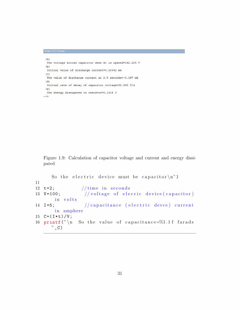
Figure 1.9: Calculation of capacitor voltage and current and energy dissi-pated
So the e l e c t r i c d e v i c e must be c a p a c i t o r \n”)11
12 t=2; // t ime i n s e c o n d s13 V=100; // v o l t a g e o f e l e c r i c d e v i c e ( c a p a c i t o r )
i n v o l t s14 I=5; // c a p a c i t a n c e ( e l e c t r i c devce ) c u r r e n t
i n amphere15 C=(I*t)/V;
16 printf(”\n So the v a l u e o f c a p a c i t a n c e=%1 . 1 f f a r a d s”,C)
31
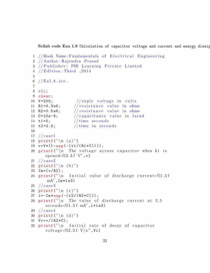
Scilab code Exa 1.8 Calculation of capacitor voltage and current and energy dissipated
1 // Book Name : Fundamentals o f E l e c t r i c a l E n g i n e e r i n g2 // Author : Rajendra Prasad3 // P u b l i s h e r : PHI Lea rn ing P r i v a t e L imi ted4 // E d i t i o n : Third ,20145
6 // Ex1 8 . s c e .7
8 clc;
9 clear;
10 V=200; // s u p l y v o l t a g e i n v o l t s11 R1=0.3e6; // r e s i s t a n c e v a l u e i n ohms12 R2=0.5e6; // r e s i s t a n c e v a l u e i n ohms13 C=10e-6; // c a p a c i t a n c e v a l u e i n f a r a d14 t1=5; // t ime s e c o n d s15 t2=2.5; // t ime i n s e c o n d s16
17 // c a s e 118 printf(”\n ( a ) ”)19 v=V*(1-exp(-(t1/(R1*C))));
20 printf(”\n The v o l t a g e a c r o s s c a p a c i t o r when k1 i sopened=%3 . 3 f V”,v)
21 // c a s e 222 printf(”\n ( b ) ”)23 Im=(v/R2);
24 printf(”\n I n i t i a l v a l u e o f d i s c h a r g e c u r r e n t=%1 . 5 fmA”,Im*1e3)
25 // c a s e 326 printf(”\n ( c ) ”)27 i=-Im*exp(-(t2/(R2*C)));
28 printf(”\n The v a l u e o f d i s c h a r g e c u r r e n t at 2 . 5s e c o n d s=%1 . 3 f mA”,i*1e3)
29 // c a s e 430 printf(”\n ( d ) ”)31 Vc=v/(R2*C);
32 printf(”\n I n i t i a l r a t e o f decay o f c a p a c i t o rv o l t a g e=%2 . 3 f V/ s ”,Vc)
32

Figure 1.10: Determination of equivalent capacitance value
33 // c a s e 534 printf(”\n ( e ) ”)35 E=(1/2) *(C*v^2);
36 printf(”\n The ene rgy d i s s i p a t e d i n r e s i s t o r=%1 . 4 fJ”,E)
Scilab code Exa 1.9 Determination of equivalent capacitance value
1 // Book Name : Fundamentals o f E l e c t r i c a l E n g i n e e r i n g2 // Author : Rajendra Prasad3 // P u b l i s h e r : PHI Lea rn ing P r i v a t e L imi ted4 // E d i t i o n : Third ,20145
6 // Ex1 9 . s c e .7
8 clc;
9 clear;
33

Figure 1.11: Plotting voltage and power and energy waveform
10 C1=100; // c a p a c i t a n c e v a l u e i n m i c r o f a r a d11 C2=150; // c a p a c i t a n c e v a l u e i n m i c r o f a r a d12 C3=200; // c a p a c i t a n c e v a l u e i n m i c r o f a r a d13
14 //CASE115 printf(”\n ( a ) ”)16 Cs=(C1*C2*C3)/((C2*C3)+(C1*C2)+(C3*C1));
17 printf(”\n The e q u i v a l e n t c a p a c i t a n c e i n s e r i e sc o n n e c t i o n=%2 . 3 f m i c r o f a r a d ”,Cs)
18
19 //CASE220 printf(”\n ( b ) ”)21 Cp=C1+C2+C3;
22 printf(”\n The e q u i v a l e n t c a p a c i t a n c e i n p a r a l l e lc o n n e c t i o n=%3 . 0 f m i c r o f a r a d ”,Cp)
Scilab code Exa 1.10 Plotting voltage and power and energy waveform
34
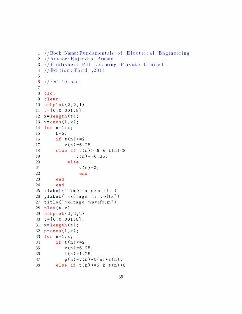
1 // Book Name : Fundamentals o f E l e c t r i c a l E n g i n e e r i n g2 // Author : Rajendra Prasad3 // P u b l i s h e r : PHI Lea rn ing P r i v a t e L imi ted4 // E d i t i o n : Third ,20145
6 // Ex1 10 . s c e .7
8 clc;
9 clear;
10 subplot (2,2,1)
11 t=[0:0.001:8];
12 x=length(t);
13 v=ones(1,x);
14 for n=1:x;
15 L=5;
16 if t(n) <=2
17 v(n)=6.25;
18 else if t(n) >=6 & t(n)<8
19 v(n)= -6.25;
20 else
21 v(n)=0;
22 end
23 end
24 end
25 xlabel(”Time i n s e c o n d s ”)26 ylabel(” v o l t a g e i n v o l t s ”)27 title(” v o l t a g e waveform ”)28 plot(t,v)
29 subplot (2,2,2)
30 t=[0:0.001:8];
31 x=length(t);
32 p=ones(1,x);
33 for n=1:x;
34 if t(n) <=2
35 v(n)=6.25;
36 i(n)=1.25;
37 p(n)=v(n)*t(n)*i(n);
38 else if t(n) >=6 & t(n)<8
35

39 v(n)= -6.25;
40 i(n)=10;
41 p(n)=(i(n) -(1.25*t(n)))*v(n);
42 else
43 v(n)=0;
44 i(n)=2.5;
45 p(n)=v(n)*t(n)*i(n);
46 end
47 end
48 end
49 xlabel(”Time i n s e c o n d s ”)50 ylabel(” power i n watt s ”)51 title(” power waveform ”)52 plot(t,p)
53 subplot (2,2,3)
54 t=[0:0.001:8];
55 x=length(t);
56 e=ones(1,x);
57 L=5;
58 for n=1:x;
59 if t(n) <=2
60 i(n)=1.25;
61 e(n)=(1/2)*L*(t(n)*i(n))^2;
62 else if t(n) >=6 & t(n)<8
63 i(n)=10;
64 e(n)=(1/2)*L*(i(n) -(1.25*t(n)))^2;
65 else
66 i(n)=2.5;
67 e(n)=(1/2)*L*(i(n))^2;
68 end
69 end
70 end
71 xlabel(”Time i n s e c o n d s ”)72 ylabel(” Energy i n j o u l e s ”)73 title(” Energy waveform ”)74 plot(t,e)
36
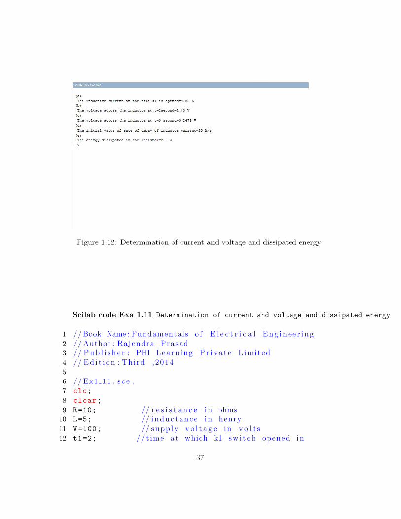
Figure 1.12: Determination of current and voltage and dissipated energy
Scilab code Exa 1.11 Determination of current and voltage and dissipated energy
1 // Book Name : Fundamentals o f E l e c t r i c a l E n g i n e e r i n g2 // Author : Rajendra Prasad3 // P u b l i s h e r : PHI Lea rn ing P r i v a t e L imi ted4 // E d i t i o n : Third ,20145
6 // Ex1 11 . s c e .7 clc;
8 clear;
9 R=10; // r e s i s t a n c e i n ohms10 L=5; // i n d u c t a n c e i n henry11 V=100; // supp ly v o l t a g e i n v o l t s12 t1=2; // t ime at which k1 s w i t c h opened i n
37

s e c o n d s13 //CASE114 printf(”\n ( a ) ”)15 i=(V*(1-exp(-((R*t1)/L))))/R;
16 printf(”\n The i n d u c t i v e c u r r e n t at the t ime k1 i sopened=%1 . 2 f A”,i)
17
18 //CASE219 printf(”\n ( b ) ”)20 v1=V*exp(-((R*t1))/L);
21 printf(”\n The v o l t a g e a c r o s s the i n d u c t o r at t=2second=%1 . 2 f V”,v1)
22
23 //CASE324 printf(”\n ( c ) ”)25 t2=3; // t ime i n s e c o n d s26 Imax=(V/R);
27 v2=Imax*R*(exp(-((R*t2))/L));
28 printf(”\n The v o l t a g e a c r o s s the i n d u c t o r at t=3second=%1 . 4 f V”,v2)
29 // For v2 c a l c u l a t i o n , the answer i n the book i swrong
30
31 //CASE432 printf(”\n ( d ) ”)33 t3=0; // i n i t i a l t ime i n s e c o n d s34 it=(-R*(-Imax)*exp(-(R*t3)/L))/L; // r a t e o f decay
o f i n d u c t o r c u r r e n t i n amphere per s e c o n d s35 printf(”\n The i n i t i a l v a l u e o f r a t e o f decay o f
i n d u c t o r c u r r e n t=%d A/ s ”,it)36
37 //CASE538 printf(”\n ( e ) ”)39 Energy =(1/2)*L*Imax ^2;
40 printf(”\n The ene rgy d i s s i p a t e d i n the r e s i s t o r=%dJ”,Energy)
38

Chapter 2
Circuit Analysis ResistiveNetwork
Scilab code Exa 2.1 Determination of unknown currents and voltages
1 // Book Name : Fundamentals o f E l e c t r i c a l E n g i n e e r i n g2 // Author : Rajendra Prasad3 // P u b l i s h e r : PHI Lea rn ing P r i v a t e L imi ted4 // E d i t i o n : Third ,20145
6 // Ex2 1 . s c e .7
8 clc;
9 clear;
10 R1=3; // R e s i s t a n c e i n ohm11 R2=5; // R e s i s t a n c e i n ohm12 R3=4; // R e s i s t a n c e i n ohm13 R4=8; // R e s i s t a n c e i n ohm14
15 I2=1/3;
16 I1=4*I2;
17 I3=I1-I2;;
39
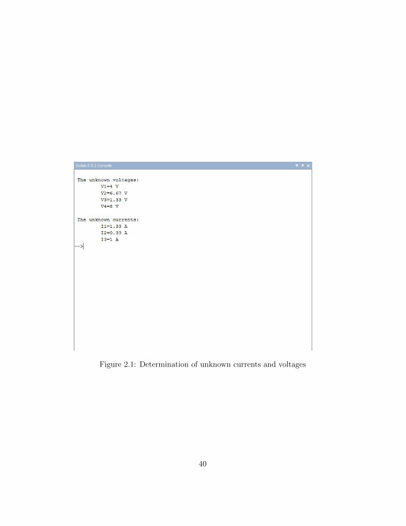
Figure 2.1: Determination of unknown currents and voltages
40

18 V1=R1*I1; // Apply ing ohm ’ s law (V=IR )
19 V2=R2*I1;
20 V3=R3*I2;
21 V4=R4*I3;
22 printf(”\n The unknown v o l t a g e s : ”)23 printf(”\n\ t V1=%d V”,V1)24 printf(”\n\ t V2=%1 . 2 f V”,V2)25 printf(”\n\ t V3=%1 . 2 f V”,V3)26 printf(”\n\ t V4=%d V \n”,V4)27 printf(”\n The unknown c u r r e n t s : ”)28 printf(”\n\ t I 1=%1 . 2 f A”,I1)29 printf(”\n\ t I 2=%1 . 2 f A”,I2)30 printf(”\n\ t I 3=%d A”,I3)
Scilab code Exa 2.2 Determination of currents in the given network
1 // Book Name : Fundamentals o f E l e c t r i c a l E n g i n e e r i n g2 // Author : Rajendra Prasad3 // P u b l i s h e r : PHI Lea rn ing P r i v a t e L imi ted4 // E d i t i o n : Third ,20145
6 // Ex2 2 . s c e .7
8 clc;
9 clear;
10 a1=2;b1=1;c1=5;d1=1; // t h e s ea r e the c o e f f i c i e n t v a l u e s o f I1 , I2 , I 3 and s o u r c e
o b t a i n e d from loop ABDA i n the g i v e n c i r c u i t11 a2=4;b2=-5;c2=-3;d2=0; // t h e s e
a r e the c o e f f i c i e n t v a l u e s o f I1 , I2 , I 3 and s o u r c eo b t a i n e d from loop ABCA i n the g i v e n c i r c u i t
12 a3=4;b3=1;c3=-9;d3=0; // t h e s e
41

Figure 2.2: Determination of currents in the given network
42

a r e the c o e f f i c i e n t v a l u e s o f I1 , I2 , I 3 and s o u r c eo b t a i n e d from loop BCDB i n the g i v e n c i r c u i t
13
14 del=det([a1 b1 c1;a2 b2 c2;a3 b3 c3]);
15 del1=det([d1 b1 c1;d2 b2 c2;d3 b3 c3]);
16 del2=det([a1 d1 c1;a2 d2 c2;a3 d3 c3]);
17 del3=det([a1 b1 d1;a2 b2 d2;a3 b3 d3]);
18
19 I1=del1/del; // UsingCramer ’ s r u l e
20 I2=del2/del; // UsingCramer ’ s r u l e
21 I3=del3/del; // UsingCramer ’ s r u l e
22
23 printf(”\n The c u r r e n t v a l u e s are , ”)24 printf(”\n\ t I 1=%1 . 1 f A”,I1)25 printf(”\n\ t I 2=%1 . 1 f A”,I2)26 printf(”\n\ t I 3=%1 . 1 f A”,I3)
Scilab code Exa 2.3 Conversion of current source into a voltage source and voltage source into a current source
1 // Book Name : Fundamentals o f E l e c t r i c a l E n g i n e e r i n g2 // Author : Rajendra Prasad3 // P u b l i s h e r : PHI Lea rn ing P r i v a t e L imi ted4 // E d i t i o n : Third ,20145
6 // Ex2 3 . s c e .7
8 clc;
9 clear;
10 // c a s e 111 // v o l t a g e s o u r c e s e r i e s with the r e s i s t a n c e
43

Figure 2.3: Conversion of current source into a voltage source and voltagesource into a current source
44

c o n v e r t e d i n t o c u r r e n t s o u r c e p a r a l l e l to theconductance
12 printf(”\n ( a ) ”)13 Rs1 =5;
14 Vs1 =100;
15 Is1=Vs1/Rs1;
16 Gs1 =1/Rs1;
17 printf(”\n I s 1=%d A \n”,Is1)18 printf(”\n Gs1=%1 . 2 f mho \n”,Gs1)19
20 // c a s e 221 // c u r r e n t s o u r c e p a r a l l e l to the conductance
c o n v e r t e d i n t o v o l t a g e s o u r c e s e r i e s with ther e s i s t a n c e
22 printf(”\n ( b ) ”)23 Gs2 =10e-3;
24 Is2 =500e-3;
25 Vs2=Is2/Gs2;
26 Rs2 =1/Gs2;
27 printf(”\n Vs2=%d V \n”,Vs2)28 printf(”\n Rs2=%d ohm \n”,Rs2)
Scilab code Exa 2.4 Determination of voltage and current using nodal analysis method
1 // Book Name : Fundamentals o f E l e c t r i c a l E n g i n e e r i n g2 // Author : Rajendra Prasad3 // P u b l i s h e r : PHI Lea rn ing P r i v a t e L imi ted4 // E d i t i o n : Third ,20145
6 // Ex2 4 . s c e .7
8 clc;
9 clear;
45
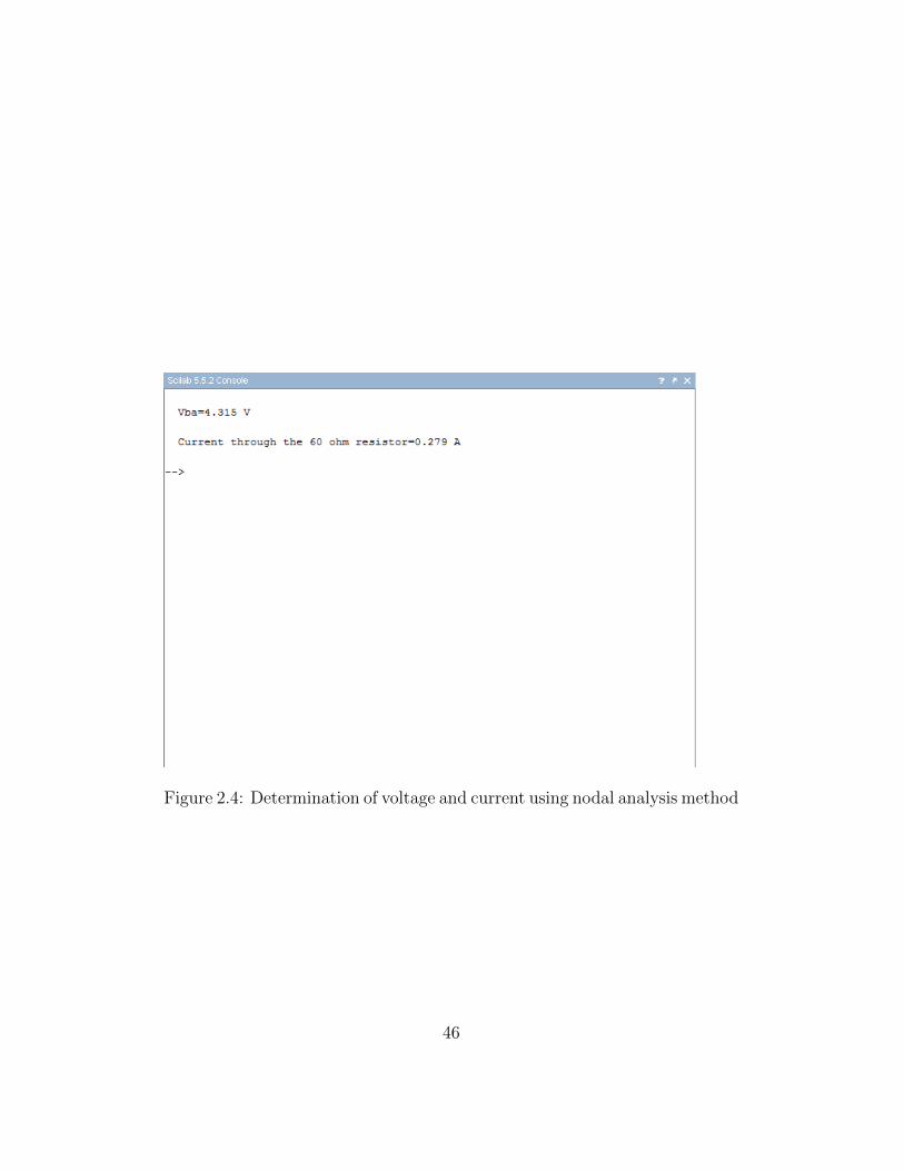
Figure 2.4: Determination of voltage and current using nodal analysis method
46

10 R5=60;
11 a1=9;b1=-5;c1=0;d1=80; // t h e s e a r ethe c o e f f i c i e n t v a l u e s o f VA,VB,VC and thes o u r c e o b t a i n e d from node A i n the g i v e n c i r c u i t
12 a2=-1;b2=7;c2=-2;d2=24; // t h e s e a r ethe c o e f f i c i e n t v a l u e s o f VA,VB,VC and thes o u r c e o b t a i n e d from node B i n the g i v e n c i r c u i t
13 a3=0;b3=-3;c3=4;d3=36; // t h e s e a r ethe c o e f f i c i e n t v a l u e s o f VA,VB,VC and thes o u r c e o b t a i n e d from node C i n the g i v e n c i r c u i t
14
15 del=det([a1 b1 c1;a2 b2 c2;a3 b3 c3]);
16 del1=det([d1 b1 c1;d2 b2 c2;d3 b3 c3]);
17 del2=det([a1 d1 c1;a2 d2 c2;a3 d3 c3]);
18 del3=det([a1 b1 d1;a2 b2 d2;a3 b3 d3]);
19
20 VA=del1/del; // UsingCramer ’ s r u l e
21 VB=del2/del; // UsingCramer ’ s r u l e
22 VC=del3/del; // UsingCramer ’ s r u l e
23 Vba=VA -VB;
24 I5=VC/R5; // from Ohm’ slaw
25 printf(”\n Vba=%1 . 3 f V \n”,Vba)26 // Answer vary dueto round o f f e r r o r27 printf(”\n Current through the 60 ohm r e s i s t o r=%1 . 3
f A \n”,I5)
Scilab code Exa 2.5 Determination of voltage and current using nodal method
1 // Book Name : Fundamentals o f E l e c t r i c a l E n g i n e e r i n g
47

Figure 2.5: Determination of voltage and current using nodal method
48

2 // Author : Rajendra Prasad3 // P u b l i s h e r : PHI Lea rn ing P r i v a t e L imi ted4 // E d i t i o n : Third ,20145
6 // Ex2 5 . s c e .7
8 clc;
9 clear;
10 R1=10;
11 R2=30;
12 R3=15;
13 R4=45;
14
15 a1=3;b1=-1;c1=-9;
// t h e s e a r e the c o e f f i c i e n t v a l u e s o f VA,VB andthe s o u r c e o b t a i n e d from node A i n the g i v e nc i r c u i t
16 a2=-3;b2=4;c2=-27;
// t h e s e a r e the c o e f f i c i e n t v a l u e s o f VA,VB andthe s o u r c e o b t a i n e d from node B i n the g i v e nc i r c u i t
17 del=det([a1 b1;a2 b2]);
18 del1=det([c1 b1;c2 b2]);
19 del2=det([a1 c1;a2 c2]);
20
21 VA=del1/del; //Using Cramer ’ s r u l e
22 VB=del2/del; // UsingCramer ’ s r u l e
23 Vba=VA -VB;
24 I2=VA/R2; // fromOhm’ s law
25 printf(”\n Vba=%d V \n”,Vba)26 printf(”\n Current through the 30 ohm r e s i s t o r=%1 . 4
f A \n”,I2)
49
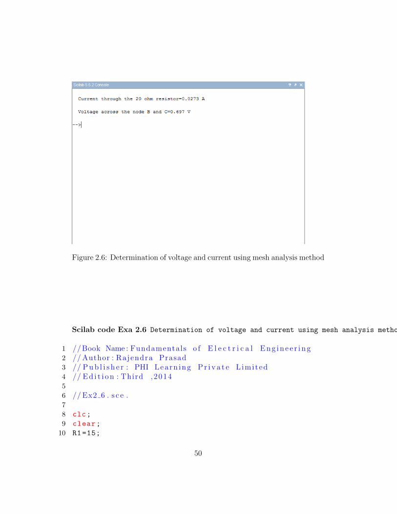
Figure 2.6: Determination of voltage and current using mesh analysis method
Scilab code Exa 2.6 Determination of voltage and current using mesh analysis method
1 // Book Name : Fundamentals o f E l e c t r i c a l E n g i n e e r i n g2 // Author : Rajendra Prasad3 // P u b l i s h e r : PHI Lea rn ing P r i v a t e L imi ted4 // E d i t i o n : Third ,20145
6 // Ex2 6 . s c e .7
8 clc;
9 clear;
10 R1=15;
50

11 R2=20;
12 R3=10;
13 R4=5;
14
15 a1=35;b1=-20;c1=2; //t h e s e a r e the c o e f f i c i e n t v a l u e s o f I1 , I 2 ands o u r c e o b t a i n e d from loop ABDA i n the g i v e nc i r c u i t
16 a2=-20;b2=35;c2 =0.5; //t h e s e a r e the c o e f f i c i e n t v a l u e s o f I1 , I 2 ands o u r c e o b t a i n e d from loop BCDB i n the g i v e nc i r c u i t
17 del=det([a1 b1;a2 b2]);
18 del1=det([c1 b1;c2 b2]);
19 del2=det([a1 c1;a2 c2]);
20
21 I1=del1/del; //Using Cramer ’ s r u l e
22 I2=del2/del; //Using Cramer ’ s r u l e
23 I20=I1 -I2;
24 Vcb=R3*I2;
25 printf(”\n Current through the 20 ohm r e s i s t o r=%1 . 4f A \n”,I20)
26 printf(”\n Vo l tage a c r o s s the node B and C=%1. 3 f V\n”,Vcb)
Scilab code Exa 2.7 Determination of voltage using nodal analysis method
1 // Book Name : Fundamentals o f E l e c t r i c a l E n g i n e e r i n g2 // Author : Rajendra Prasad3 // P u b l i s h e r : PHI Lea rn ing P r i v a t e L imi ted4 // E d i t i o n : Third ,2014
51

Figure 2.7: Determination of voltage using nodal analysis method
52

5
6 // Ex2 7 . s c e .7
8 clc;
9 clear;
10 R1=5; // R e s i s t a n c e i n ohm11 R2=2; // R e s i s t a n c e i n ohm12 R3=3; // R e s i s t a n c e i n ohm13
14 a1=7;b1=-5;c1=50; //t h e s e a r e the c o e f f i c i e n t v a l u e s o f VA,VB and the
s o u r c e o b t a i n e d from node A i n the g i v e n c i r c u i t15 a2=3;b2=5;c2=0; //
t h e s e a r e the c o e f f i c i e n t v a l u e s o f VA,VB and thes o u r c e o b t a i n e d from node B i n the g i v e n c i r c u i t
16 del=det([a1 b1;a2 b2]);
17 del1=det([c1 b1;c2 b2]);
18 del2=det([a1 c1;a2 c2]);
19
20 VA=del1/del; //Using Cramer ’ s r u l e
21 VB=del2/del; //Using Cramer ’ s r u l e
22 Vba=VA -VB;
23 printf(”\n Vo l tage a c r o s s the 2 ohm r e s i s t o r=%d V \n”,Vba)
Scilab code Exa 2.8 Determination of current using mesh voltage method
1 // Book Name : Fundamentals o f E l e c t r i c a l E n g i n e e r i n g2 // Author : Rajendra Prasad3 // P u b l i s h e r : PHI Lea rn ing P r i v a t e L imi ted4 // E d i t i o n : Third ,2014
53
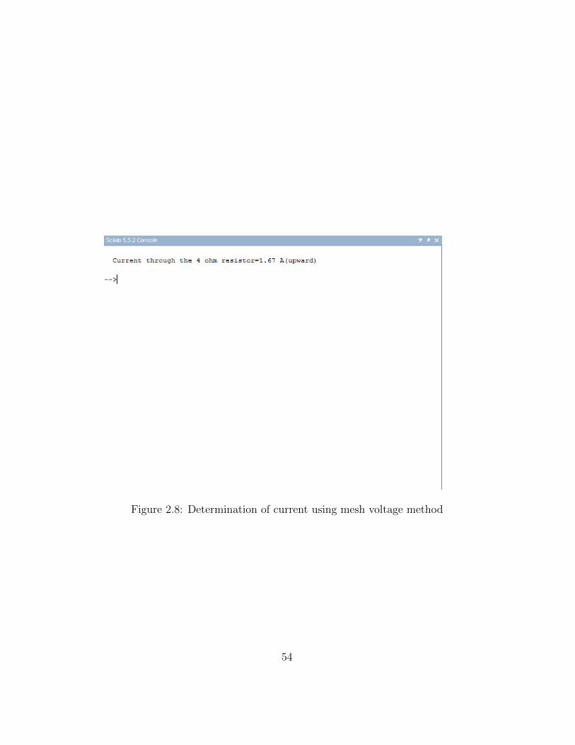
Figure 2.8: Determination of current using mesh voltage method
54

5
6 // Ex2 8 . s c e .7
8 clc;
9 clear;
10 R1=3;
11 R2=4;
12 R3=2;
13 R4=1;
14
15 a1=7;b1=-4;c1=2; //t h e s e a r e the c o e f f i c i e n t v a l u e s o f I1 , I 2 ands o u r c e o b t a i n e d from the f i r s t l o op i n the g i v e nc i r c u i t
16 a2=-10;b2=7;c2=3; //t h e s e a r e the c o e f f i c i e n t v a l u e s o f I1 , I 2 ands o u r c e o b t a i n e d from the second l oop i n theg i v e n c i r c u i t
17 del=det([a1 b1;a2 b2]);
18 del1=det([c1 b1;c2 b2]);
19 del2=det([a1 c1;a2 c2]);
20
21 I1=del1/del; // UsingCramer ’ s r u l e
22 I2=del2/del; // UsingCramer ’ s r u l e
23 I=I2 -I1;
24 printf(”\n Current through the 4 ohm r e s i s t o r=%1 . 2 fA( upward ) \n”,I)
Scilab code Exa 2.9 Determination of current using a principle of superposition
1 // Book Name : Fundamentals o f E l e c t r i c a l E n g i n e e r i n g
55
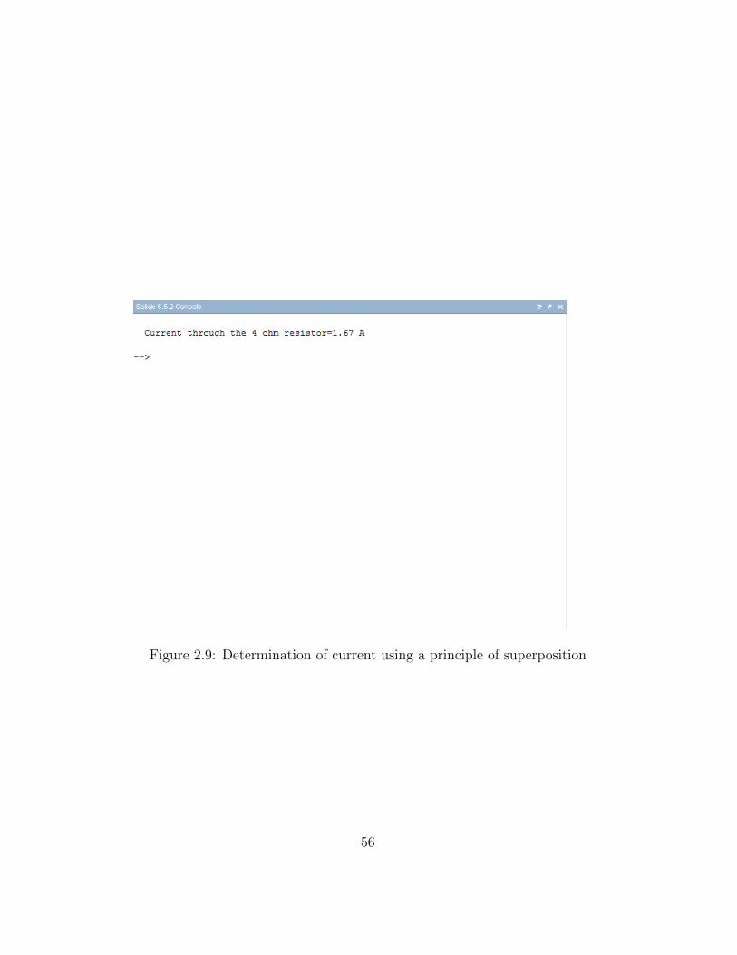
Figure 2.9: Determination of current using a principle of superposition
56

2 // Author : Rajendra Prasad3 // P u b l i s h e r : PHI Lea rn ing P r i v a t e L imi ted4 // E d i t i o n : Third ,20145
6 // Ex2 9 . s c e .7
8 clc;
9 clear;
10 R1=3;
11 R2=4;
12 R3=2;
13 R4=1;
14
15 // c a s e ( a )16 a1=13;b1=-6;c1=20;
// t h e s e a r e the c o e f f i c i e n t v a l u e s o f VA,VB ands o u r c e o b t a i n e d from the node A i n the g i v e nc i r c u i t
17 a2=-5;b2=3;c2=-20;
// t h e s e a r e the c o e f f i c i e n t v a l u e s o f VA,VB ands o u r c e o b t a i n e d from the node B i n the g i v e nc i r c u i t
18 del=det([a1 b1;a2 b2]);
19 del1=det([c1 b1;c2 b2]);
20 VA1=del1/del;
21 Idash=-VA1/R2;
22
23 // c a s e ( b )24 Vs=3;
25 a1=13;b1=-6;c1=9;
// t h e s e a r e the c o e f f i c i e n t v a l u e s o f VA,VB ands o u r c e o b t a i n e d from the node A i n the g i v e nc i r c u i t
26 a2=-5;b2=3;c2=0;
// t h e s e a r ethe c o e f f i c i e n t v a l u e s o f VA,VB and s o u r c eo b t a i n e d from the node B i n the g i v e n c i r c u i t
27 del=det([a1 b1;a2 b2]);
57

Figure 2.10: Determination of current in all resistance using superpositionprinciple
28 del1=det([c1 b1;c2 b2]);
29 VA2=del1/del;
30 I_doubledash =(Vs-VA2)/R2;
31 I=Idash+I_doubledash;
32 printf(”\n Current through the 4 ohm r e s i s t o r=%1 . 2 fA \n”,I)
Scilab code Exa 2.10 Determination of current in all resistance using superposition principle
1 // Book Name : Fundamentals o f E l e c t r i c a l E n g i n e e r i n g2 // Author : Rajendra Prasad
58

3 // P u b l i s h e r : PHI Lea rn ing P r i v a t e L imi ted4 // E d i t i o n : Third ,20145
6 // Ex2 10 . s c e .7
8 clc;
9 clear;
10 R1=4;
11 R2=3;
12 R3=5;
13 R4=6;
14
15 //CASE ( a )16 Vs1 =80;
17 VA1=(Vs1/R3)/((1/ R1)+(1/R2)+(1/R3)+(1/R4));
18 I1dash=VA1/R1; //From ohm ’ s law (V=IR )19 I2dash=VA1/R2;
20 I3dash =(Vs1 -VA1)/R3;
21 I4dash=VA1/R4;
22
23 //CASE ( b )24 Vs2 =90;
25 VA2=(Vs2/R2)/((1/ R1)+(1/R2)+(1/R3)+(1/R4));
26 I1doubledash=VA2/R1;
27 I2doubledash =(Vs2 -VA2)/R2;
28 I3doubledash=VA2/R3;
29 I4doubledash=VA2/R4;
30
31 //CASE ( c )32 Is=20;
33 VA3=Is/((1/R1)+(1/R2)+(1/R3)+(1/R4));
34 I1tripledash=VA3/R1;
35 I2tripledash=VA3/R2;
36 I3tripledash=VA3/R3;
37 I4tripledash=VA3/R4;
38 I1=I1dash+I1doubledash+I1tripledash;
39 I2=-I2dash+I2doubledash -I2tripledash;
40 I3=I3dash -I3doubledash -I3tripledash;
59

Figure 2.11: Determination of current using Thevenins theorem
41 I4=I4dash+I4doubledash+I4tripledash;
42 printf(”\n Current i n 4 ohm r e s i t a n c e=%2 . 1 f A \n”,I1)
43 printf(”\n Current i n 3 ohm r e s i t a n c e=%1 . 2 f A \n”,I2)
44 printf(”\n Current i n 5 ohm r e s i t a n c e=%d A \n”,I3)45 printf(”\n Current i n 6 ohm r e s i t a n c e=%2 . 1 f A \n”,
I4)
46
47 //The answer vary dueto r o u n d o f f e r r o r
60

Scilab code Exa 2.11 Determination of current using Thevenins theorem
1 // Book Name : Fundamentals o f E l e c t r i c a l E n g i n e e r i n g2 // Author : Rajendra Prasad3 // P u b l i s h e r : PHI Lea rn ing P r i v a t e L imi ted4 // E d i t i o n : Third ,20145
6 // Ex2 11 . s c e7
8 clc;
9 clear;
10 R1=30; // R e s i s t a n c e i n ohm11 R2=60; // R e s i s t a n c e i n ohm12 R3=60; // R e s i s t a n c e i n ohm13 R4=30; // R e s i s t a n c e i n ohm14 R5=10; // R e s i s t a n c e i n ohm15 R=50; // R e s i s t a n c e i n ohm16 I1 =5/110; // Loop1 c u r r e n t i n Ampere17 I2 =5/110; // Loop2 c u r r e n t i n Ampere18 Voc=(I2*R2) -(I1*R1); //Open c i r c u i t v o l t a g e i n
Vol t19 Isc =1/30; //Open c i r c u i t c u r r e n t i n
Ampere20 Rs=Voc/Isc; // S e r i e s r e s i s t a n c e i n ohm21 I=Voc/(Rs+R);
22 printf(”\n Current through the 50 ohm r e s i s t o r=%1 . 3f A \n”,I)
Scilab code Exa 2.12 Determination of current using Norton theorem
1 // Book Name : Fundamentals o f E l e c t r i c a l E n g i n e e r i n g2 // Author : Rajendra Prasad3 // P u b l i s h e r : PHI Lea rn ing P r i v a t e L imi ted
61

Figure 2.12: Determination of current using Norton theorem
62
4 // E d i t i o n : Third ,20145
6 // Ex2 12 . s c e7
8 clc;
9 clear;
10 R=50; // R e s i s t a n c e i n ohm11 Is =1/30; // Source c u r r e n t i n Ampere12 Rs =40.92; // P a r a l l e l r e s i s t a n c e i n ohm13 Gs=1/Rs; // P a r a l l e l conductance i n mho14 I=(Is*Rs)/(Rs+R);
15 printf(”\n Current through the 50 ohm r e s i s t o r=%1 . 3f A \n”,I)
Scilab code Exa 2.13 Determination of load resistance
1 // Book Name : Fundamentals o f E l e c t r i c a l E n g i n e e r i n g2 // Author : Rajendra Prasad3 // P u b l i s h e r : PHI Lea rn ing P r i v a t e L imi ted4 // E d i t i o n : Third ,20145
6 // Ex2 13 . s c e .7
8 clc;
9 clear;
10 R1=4; // R e s i s t a n c e i n ohm11 R2=4; // R e s i s t a n c e i n ohm12 R3=8; // R e s i s t a n c e i n ohm13 R4=10; // R e s i s t a n c e i n ohm14 R5=3; // R e s i s t a n c e i n ohm15 R6=8; // R e s i s t a n c e i n ohm16 R7=2; // R e s i s t a n c e i n ohm17 R12 =1/((1/ R1)+(1/R2)); //R1 and R2 a r e i n
63

Figure 2.13: Determination of load resistance
64

Figure 2.14: Determination of driving point resistance of the voltage source
p a r a l l e l18 R34 =1/((1/ R4)+(1/( R3+R12))); //R12 and R3 a r e i n
p a r a l l e l with R419 R56 =1/((1/ R6)+(1/( R5+R34))); //R34 and R5 a r e i n
p a r a l l e l with R620 Rab=R7+R56; //R56 and R7 a r e i n s e r i e s21 RL=Rab;
22 printf(”\n Load r e s i t a n c e to the 10 v o l t s o u r c e=%dohm \n”,RL )
65

Scilab code Exa 2.14 Determination of driving point resistance of the voltage source
1 // Book Name : Fundamentals o f E l e c t r i c a l E n g i n e e r i n g2 // Author : Rajendra Prasad3 // P u b l i s h e r : PHI Lea rn ing P r i v a t e L imi ted4 // E d i t i o n : Third ,20145
6 // Ex2 14 . s c e7
8 clc;
9 clear;
10 I=5/31; // C i r c u i t c u r r e n t i n ampere11 Vs=5; // Source v o l t a g e i n v o l t12 R1=3; // R e s i s t a n c e i n ohm13 R2=4; // R e s i s t a n c e i n ohm14 driving_point_resistance=Vs/I;
15 printf(”\n The d r i v i n g p o i n t r e s i s t a n c e o f thev o l t a g e s o u r c e=%d ohm \n”,driving_point_resistance)
Scilab code Exa 2.15 Determination of driving point resistance at the pair of terminals
1 // Book Name : Fundamentals o f E l e c t r i c a l E n g i n e e r i n g2 // Author : Rajendra Prasad3 // P u b l i s h e r : PHI Lea rn ing P r i v a t e L imi ted4 // E d i t i o n : Third ,20145
6 // Ex2 15 . s c e .7
8 clc;
66

Figure 2.15: Determination of driving point resistance at the pair of terminals
67

9 clear;
10 R_aB =5;
11 R_AB =6;
12 R_BC =6;
13 R_CD =5;
14 R_AE =25;
15 R_ED =10;
16 R_DA =5;
17 R_EC =50;
18
19 // For t r i a n g l e AED20 R_OA=(R_AE*R_DA)/(R_AE+R_ED+R_DA);
21 R_OD=(R_ED*R_DA)/(R_AE+R_ED+R_DA);
22 R_OE=(R_AE*R_ED)/(R_AE+R_ED+R_DA);
23
24 // For t r i a n g l e OCD25 R_OC=R_OE+R_EC;
26 R_OdashO =(R_OC*R_OD)/(R_OC+R_OD+R_CD);
27 R_OdashD =(R_CD*R_OD)/(R_OC+R_OD+R_CD);
28 R_OdashC =(R_OC*R_CD)/(R_OC+R_OD+R_CD);
29
30 R_OB=R_OA+R_AB;
31 R_BOdash =(( R_OB+R_OdashO)*(R_BC+( R_OdashC)))/(R_OB+
R_OdashO+R_BC+R_OdashC);
32 Rab=(R_aB+( R_BOdash)+( R_OdashD));
33 printf(”\n The d r i v i n g p o i n t r e s i s t a n c e=%2 . 1 f ohms\n”,Rab)
Scilab code Exa 2.16 Determination of resistance value and amount of power
1 // Book Name : Fundamentals o f E l e c t r i c a l E n g i n e e r i n g2 // Author : Rajendra Prasad3 // P u b l i s h e r : PHI Lea rn ing P r i v a t e L imi ted
68

Figure 2.16: Determination of resistance value and amount of power
69
4 // E d i t i o n : Third ,20145
6 // Ex2 16 . s c e .7
8 clc;
9 clear;
10 R1=10;
11 I1=2.5;
12 V2=60;
13 R2=30;
14 I2=V2/R2; //Ohm’ s law15 Gs=(1/R1)+(1/R2);
16 Rs=1/Gs;
17 Isc=I1+I2;
18 Voc=Isc*Rs;
19
20 // c a s e ( a )21 printf(”\n ( a ) ”)22 R=Rs;
23 printf(”\n The v a l u e o f R which a b s o r b s maximumpower from the c i r c u i t=%1 . 1 f ohm \n”,R)
24
25 // c a s e ( b )26 printf(”\n ( b ) ”)27 Pm=Voc ^2/(4* Rs);
28 printf(”\n The amount o f power=%2 . 0 f W \n”,Pm)
70

Chapter 3
Circuit Analysis Time VaryingExcitation
Scilab code Exa 3.1 Calculation of impedence and admittance
1 // Book Name : Fundamentals o f E l e c t r i c a l E n g i n e e r i n g2 // Author : Rajendra Prasad3 // P u b l i s h e r : PHI Lea rn ing P r i v a t e L imi ted4 // E d i t i o n : Third ,20145
6 // Ex3 1 . s c e7
8 clc;
9 clear;
10 L=2.5;
11 s=-1; // complex f r e q u e n c y , which i s taken from thec o e f f i c i e n t v a l u e o f t ime i n the g i v e ne x p o n e n t i a l term
12 Z=L*s;
13 printf(”\n Impedence=%1 . 1 f ohm \n”,Z)14 Y=1/Z;
15 printf(”\n Admittance=%0 . 1 f mho \n”,Y)
71

Figure 3.1: Calculation of impedence and admittance
16 // Vo l tage cannot be dete rmined s i n c e i t i n v o l v e se q u a t i o n i n the r e s u l t
Scilab code Exa 3.3 Determination of voltage across resistance and inductance and capacitance
1 // Book Name : Fundamentals o f E l e c t r i c a l E n g i n e e r i n g2 // Author : Rajendra Prasad3 // P u b l i s h e r : PHI Lea rn ing P r i v a t e L imi ted4 // E d i t i o n : Third ,20145
6 // Ex3 3 ( b ) . s c e .7
8 clc;
9 clear;
10 R=1;
11 L=1;
12 C=0.1;
13 // c a s e ( b )
72

Figure 3.2: Determination of voltage across resistance and inductance andcapacitance
14 s=0;
15 //Z=R+(L∗ s ) +(1/(C∗ s ) )16 Z=0; //Z=s /( s ˆ2+ s +10)17 // v o l t a g e a c r o s s the r e s i s t a n c c e and i n d u c t a n c e a r e
z e r o18
19 Vc =100/(s^2+s+10);// s i m p l i f i e d form o f (10 s /( s ˆ2+ s+10) ) / ( 0 . 1 s )
20 printf(”\n Vo l tage a c r o s s the c a p a c i t a n c e=%d v o l t ”,Vc)
Scilab code Exa 3.4 Determination of current through conductance and capacitance and inductance
1 // Book Name : Fundamentals o f E l e c t r i c a l E n g i n e e r i n g2 // Author : Rajendra Prasad3 // P u b l i s h e r : PHI Lea rn ing P r i v a t e L imi ted
73
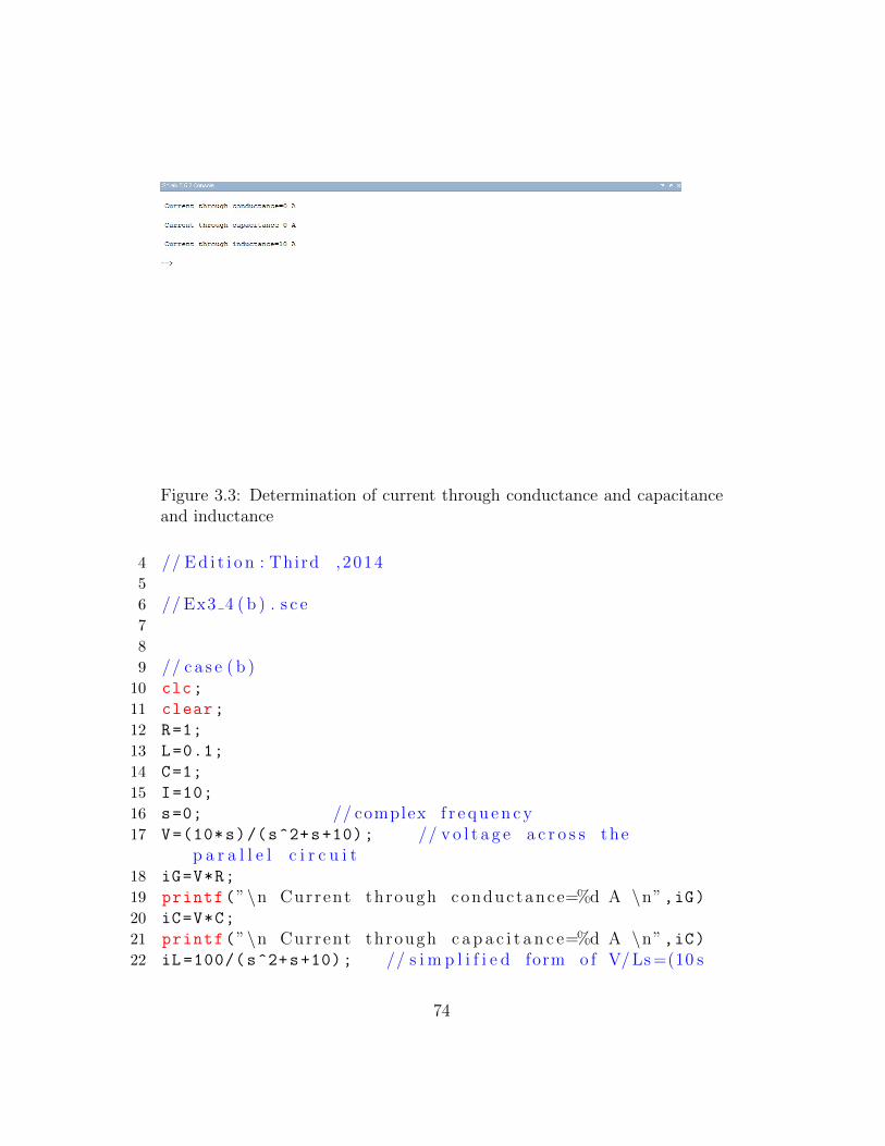
Figure 3.3: Determination of current through conductance and capacitanceand inductance
4 // E d i t i o n : Third ,20145
6 // Ex3 4 ( b ) . s c e7
8
9 // c a s e ( b )10 clc;
11 clear;
12 R=1;
13 L=0.1;
14 C=1;
15 I=10;
16 s=0; // complex f r e q u e n c y17 V=(10*s)/(s^2+s+10); // v o l t a g e a c r o s s the
p a r a l l e l c i r c u i t18 iG=V*R;
19 printf(”\n Current through conductance=%d A \n”,iG)20 iC=V*C;
21 printf(”\n Current through c a p a c i t a n c e=%d A \n”,iC)22 iL =100/(s^2+s+10); // s i m p l i f i e d form o f V/ Ls =(10 s
74

Figure 3.4: Determination of current and voltage across inductance
/( s ˆ2+ s +10) ) / ( 0 . 1 s )23 printf(”\n Current through i n d u c t a n c e=%d A \n”,iL)
Scilab code Exa 3.5 Determination of current and voltage across inductance
1 // Book Name : Fundamentals o f E l e c t r i c a l E n g i n e e r i n g2 // Author : Rajendra Prasad3 // P u b l i s h e r : PHI Lea rn ing P r i v a t e L imi ted4 // E d i t i o n : Third ,20145
6 // Ex3 5 . s c e
75

7
8 clc;
9 clear;
10 R=2;
11 L=2;
12 C=1/12;
13 omega =3;
14 XL=omega*L;
15 XC=1/( omega*C);
16 Z=complex(R,XL -XC);
17 Vl=12* sqrt (2);
18 theta =30;
19 V=complex(Vl*cosd(theta),Vl*sind(theta));
20 I=V/Z;
21 I_mag=sqrt(real(I)^2+ imag(I)^2);
22 I_angle=atand(imag(I)/real(I));
23 printf(”\n Current f l o w through the g i v e n c i r c u i t=%da n g l e :%d d e g r e e \n”,I_mag ,I_angle)
24
25 XL=complex (0,6);
26 V_L=I*XL;
27 V_L_mag=sqrt(real(V_L)^2+ imag(V_L)^2);
28 V_L_angle=atand(imag(V_L)/real(V_L));
29 printf(”\n Vo l tage a c r o s s the i n d u c t a n c e=%d a n g l e : %2. 0 f d e g r e e \n”,V_L_mag ,V_L_angle)
30 // r e s u l t : Vl ( t ) =36 s i n ( wt+75) , i ( t )=6 s i n ( wt−15)
Scilab code Exa 3.6 Determination of forced component of current
1 // Book Name : Fundamentals o f E l e c t r i c a l E n g i n e e r i n g2 // Author : Rajendra Prasad3 // P u b l i s h e r : PHI Lea rn ing P r i v a t e L imi ted4 // E d i t i o n : Third ,2014
76
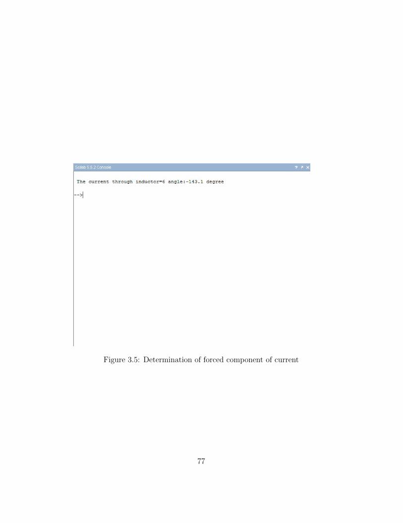
Figure 3.5: Determination of forced component of current
77

5
6 // Ex3 6 . s c e7
8 clc;
9 clear;
10 G=3; // conductance i n mho11 L=1/4; // I n d u c t o r v a l u e i n henry12 C=3; // c a p a c i t o r v a l u e i n f a r a d13 omega =2; // taken from i ( t )14 XL=1/( omega*L);
15 XC=( omega*C);
16 Y=complex(G,XC -XL);
17 I=complex (15 ,0);
18 V=I/Y;
19 BL= complex (0,-2);
20 I_L=V*BL;
21 I_L_mag=sqrt(real(I_L)^2+ imag(I_L)^2);
22 I_L_angle=atand(imag(I_L)/real(I_L)) -180;
23 printf(”\n The c u r r e n t through i n d u c t o r=%d a n g l e : %2. 1 f d e g r e e \n”,I_L_mag ,I_L_angle)
24 // r e s u l t : iL ( t )=6 co s (2 t −143 .1)
Scilab code Exa 3.7 Determination of average and RMS value of voltage
1 // Book Name : Fundamentals o f E l e c t r i c a l E n g i n e e r i n g2 // Author : Rajendra Prasad3 // P u b l i s h e r : PHI Lea rn ing P r i v a t e L imi ted4 // E d i t i o n : Third ,20145
6 // Ex3 7 . s c e7
8 clc;
9 clear;
78

Figure 3.6: Determination of average and RMS value of voltage
10
11 printf(”\n ( a ) ”)12 T=(2* %pi); //Time v a l u e f o r one c y c l e13 V=15; //Maximum v o l t a g e i n v o l t14 t0=%pi/4;t1=%pi; // t ime v a l u e s f o r p a r t i c u l a r p e r i o d
which i s taken from the g i v e n v o l t a g e wave form15 Vav =(1/T)*integrate( ’V∗ s i n ( t ) ’ , ’ t ’ ,t0 ,t1);16 printf(”\n Average v a l u e=%1 . 3 f v o l t \n”,Vav)17
18 printf(”\n ( b ) ”)19 Vrms=sqrt (((V^2)/T)*integrate( ’ (1− co s (2∗ t ) ) /2 ’ , ’ t ’ ,
t0 ,t1)); // s i n ˆ2( t )=(1− co s (2 t ) ) /220 printf(”\n RMS v a l u e=%1 . 2 f v o l t \n”,Vrms)21 // Answer g i v e n i n the book f o r Vrms i s wrong
79

Figure 3.7: Determination of circuit current and voltage using phasor method
80

Scilab code Exa 3.8 Determination of circuit current and voltage using phasor method
1 // Book Name : Fundamentals o f E l e c t r i c a l E n g i n e e r i n g2 // Author : Rajendra Prasad3 // P u b l i s h e r : PHI Lea rn ing P r i v a t e L imi ted4 // E d i t i o n : Third ,20145
6 // EX3 8 . s c e7
8 clc;
9 clear;
10 R=2; // R e s i s t a n c e i n ohm11 L=2; // I n d u c t o r v a l u e i n henry12 C=1/12; // c a p a c i t o r v a l u e i n f a r a d13 omega =3; // Taken from v ( t ) v a l u e14 // g i v e n v ( t ) =12 s i n (3 t +30) ;15 Vm=12;
16 Vrms=Vm/sqrt (2);
17 theta =30;
18
19 Z=complex(R,(omega*L) -(1/( omega*C)));
20 V=complex(Vrms*cosd(theta),Vrms*sind(theta));
21 I=V/Z;
22 I_mag=sqrt(real(I)^2+ imag(I)^2);
23 I_ang=atand(imag(I)/real(I));
24 printf(”\n C i r c u i t c u r r e n t=%1 . 0 f a n g l e :%d d e g r e e \n”,I_mag ,I_ang)
25
26 Vr=I*R;
27 Vr_mag=sqrt(real(Vr)^2+ imag(Vr)^2);
28 Vr_ang=atand(imag(Vr)/real(Vr));
29 printf(”\n Vo l tage a c r o s s the r e s i s t a n c e=%1 . 0 f a n g l e:%d d e g r e e \n”,Vr_mag ,Vr_ang)
30
31 theta1 =90;
32 Xl=complex(omega*L*cosd(theta1),omega*L*sind(theta1)
);
33 Vl=I*Xl;
81

34 Vl_mag=sqrt(real(Vl)^2+ imag(Vl)^2);
35 Vl_ang=atand(imag(Vl)/real(Vl));
36 printf(”\n Vo l tage a c r o s s the i n d u c t a n c e=%1 . 0 f a n g l e: %1 . 0 f d e g r e e \n”,Vl_mag ,Vl_ang)
37
38 theta2 =-90;
39 Xc=complex(cosd(theta2)/( omega*C),sind(theta2)/(
omega*C));
40 Vc=I*Xc;
41 Vc_mag=sqrt(real(Vc)^2+ imag(Vc)^2);
42 Vc_ang=atand(imag(Vc)/real(Vc)) -180;
43 printf(”\n Vo l tage a c r o s s the c a p a c i t a n c e=%1 . 0 fa n g l e :%d d e g r e e \n”,Vc_mag ,Vc_ang)
Scilab code Exa 3.9 Determination of current through different elements and voltage
1 // Book Name : Fundamentals o f E l e c t r i c a l E n g i n e e r i n g2 // Author : Rajendra Prasad3 // P u b l i s h e r : PHI Lea rn ing P r i v a t e L imi ted4 // E d i t i o n : Third ,20145
6 // Ex3 9 . s c e7
8 clc;
9 clear;
10 G=3; // Conductance i n mho11 L=1/4; // I n d u c t o r v a l u e i n henry12 C=3; // c a p a c i t o r v a l u e i n f a r a d13 // Given i ( t ) =15 co s 2 t ;14 Im=15;
15 Irms=Im/sqrt (2);
16 omega =2;
17 theta =0;
82
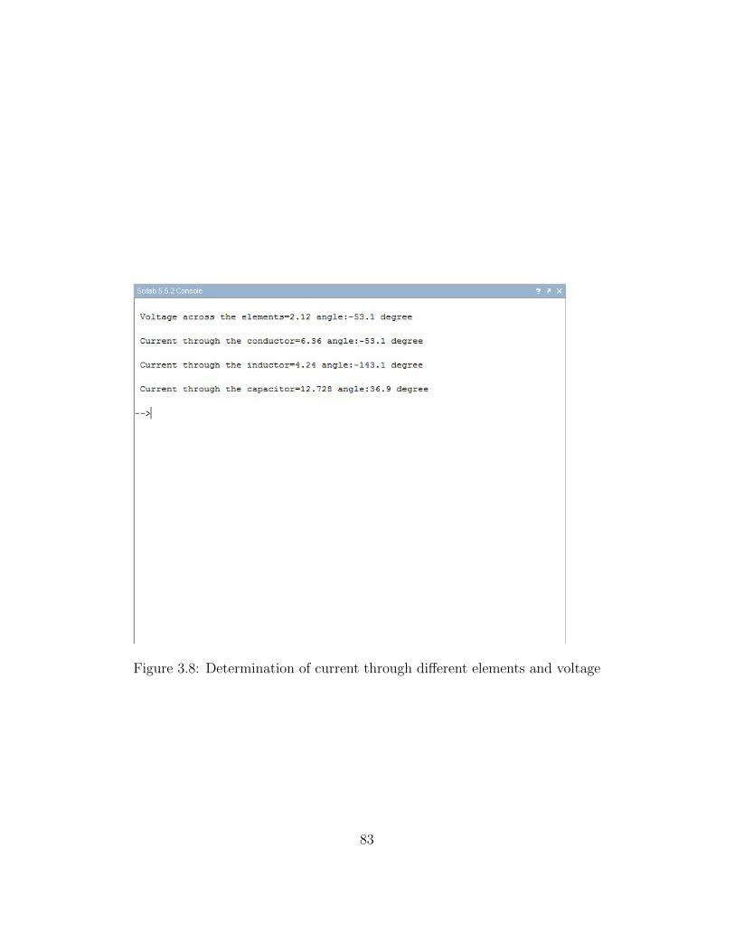
Figure 3.8: Determination of current through different elements and voltage
83

18
19 Y=complex(G,(omega*C) -(1/( omega*L)));
20 I=complex(Irms*cosd(theta),Irms*sind(theta));
21 V=I/Y;
22 V_mag=sqrt(real(V)^2+ imag(V)^2);
23 V_ang=atand(imag(V)/real(V));
24 printf(”\n Vo l tage a c r o s s the e l e m e n t s=%1 . 2 f a n g l e :%2 . 1 f d e g r e e \n”,V_mag ,V_ang)
25
26 Ig=V*G;
27 Ig_mag=sqrt(real(Ig)^2+ imag(Ig)^2);
28 Ig_ang=atand(imag(Ig)/real(Ig));
29 printf(”\n Current through the conduc to r=%1 . 2 f a n g l e: %2 . 1 f d e g r e e \n”,Ig_mag ,Ig_ang)
30
31 theta1 =-90;
32 Bl=complex(cosd(theta1)/( omega*L),sind(theta1)/(
omega*L));
33 Il=V*Bl;
34 Il_mag=sqrt(real(Il)^2+ imag(Il)^2);
35 Il_ang=atand(imag(Il)/real(Il)) -180;
36 printf(”\n Current through the i n d u c t o r=%1 . 2 f a n g l e :%3 . 1 f d e g r e e \n”,Il_mag ,Il_ang)
37
38 theta2 =90;
39 Bc=complex(cosd(theta1)*omega*C,sind(theta1)*omega*C
);
40 Ic=V*Bc;
41 Ic_mag=sqrt(real(Ic)^2+ imag(Ic)^2);
42 Ic_ang=atand(imag(Ic)/real(Ic));
43 printf(”\n Current through the c a p a c i t o r=%2 . 3 f a n g l e: %2 . 1 f d e g r e e \n”,Ic_mag ,Ic_ang)
84

Figure 3.9: Determination of voltage and current using complex method
85
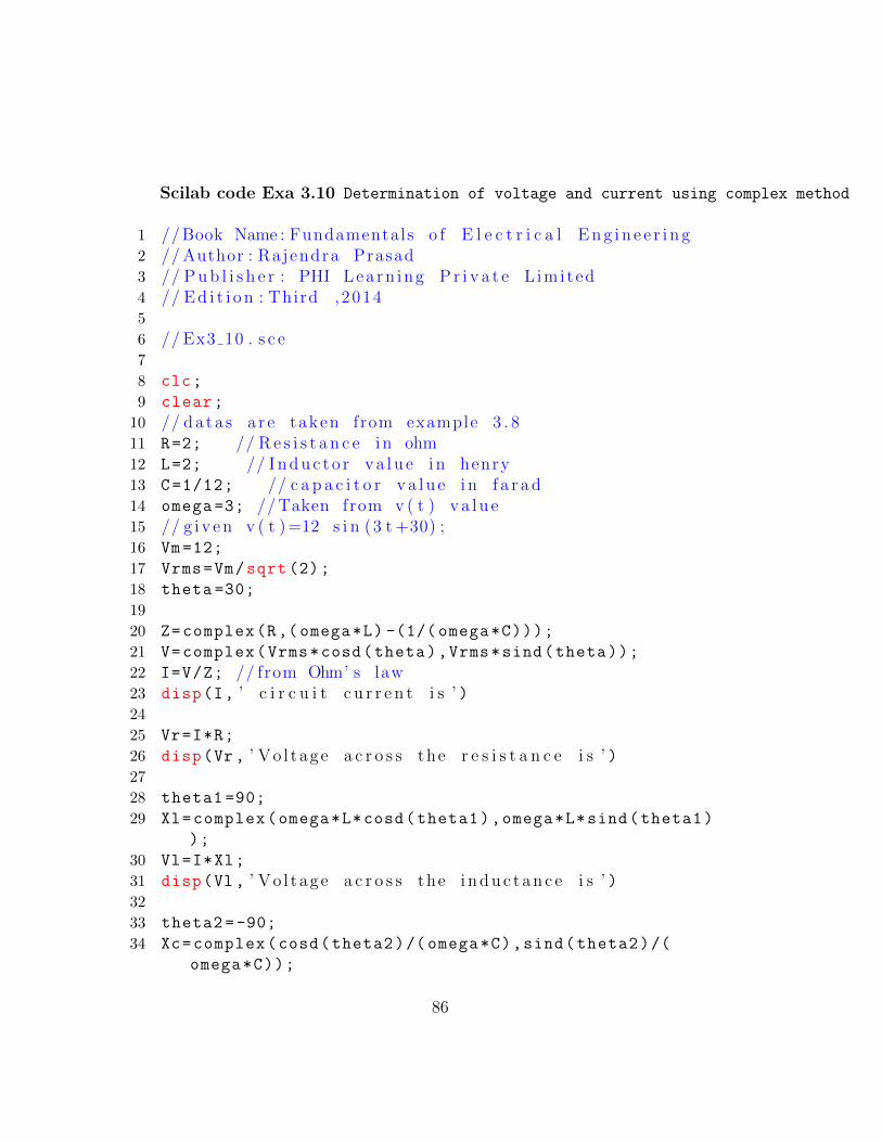
Scilab code Exa 3.10 Determination of voltage and current using complex method
1 // Book Name : Fundamentals o f E l e c t r i c a l E n g i n e e r i n g2 // Author : Rajendra Prasad3 // P u b l i s h e r : PHI Lea rn ing P r i v a t e L imi ted4 // E d i t i o n : Third ,20145
6 // Ex3 10 . s c e7
8 clc;
9 clear;
10 // da ta s a r e taken from example 3 . 811 R=2; // R e s i s t a n c e i n ohm12 L=2; // I n d u c t o r v a l u e i n henry13 C=1/12; // c a p a c i t o r v a l u e i n f a r a d14 omega =3; // Taken from v ( t ) v a l u e15 // g i v e n v ( t ) =12 s i n (3 t +30) ;16 Vm=12;
17 Vrms=Vm/sqrt (2);
18 theta =30;
19
20 Z=complex(R,(omega*L) -(1/( omega*C)));
21 V=complex(Vrms*cosd(theta),Vrms*sind(theta));
22 I=V/Z; // from Ohm’ s law23 disp(I, ’ c i r c u i t c u r r e n t i s ’ )24
25 Vr=I*R;
26 disp(Vr, ’ Vo l tage a c r o s s the r e s i s t a n c e i s ’ )27
28 theta1 =90;
29 Xl=complex(omega*L*cosd(theta1),omega*L*sind(theta1)
);
30 Vl=I*Xl;
31 disp(Vl, ’ Vo l tage a c r o s s the i n d u c t a n c e i s ’ )32
33 theta2 =-90;
34 Xc=complex(cosd(theta2)/( omega*C),sind(theta2)/(
omega*C));
86
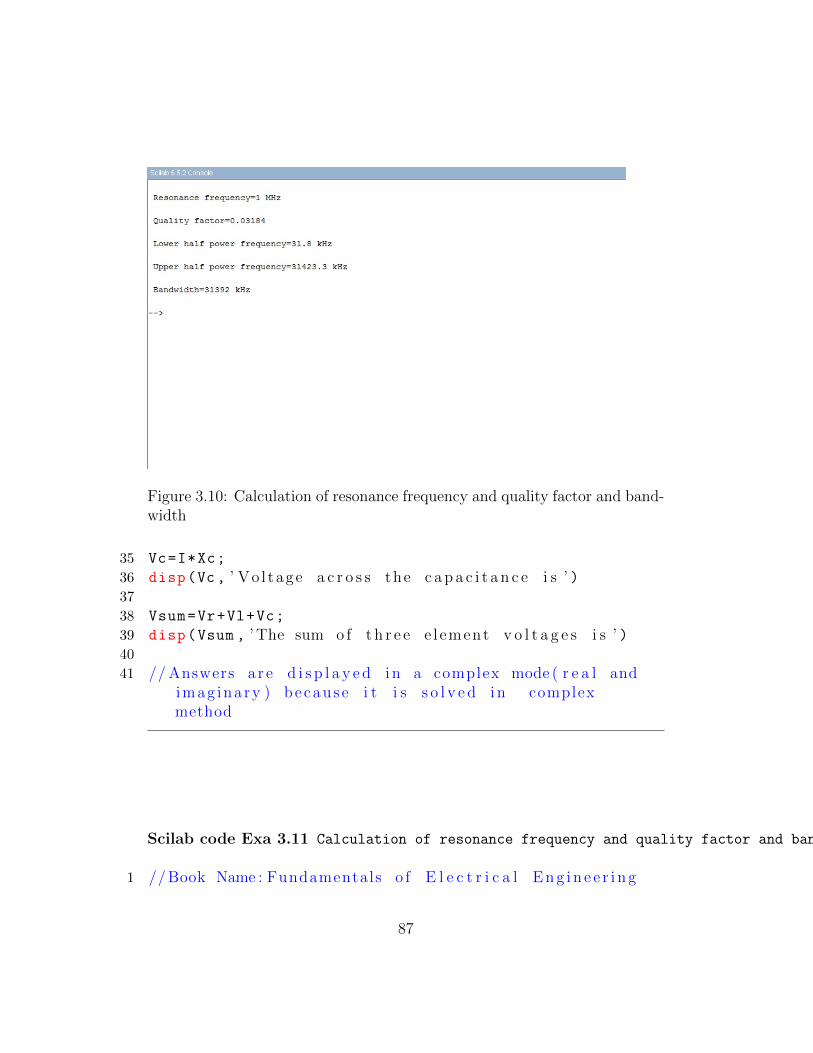
Figure 3.10: Calculation of resonance frequency and quality factor and band-width
35 Vc=I*Xc;
36 disp(Vc, ’ Vo l tage a c r o s s the c a p a c i t a n c e i s ’ )37
38 Vsum=Vr+Vl+Vc;
39 disp(Vsum , ’ The sum o f t h r e e e l ement v o l t a g e s i s ’ )40
41 // Answers a r e d i s p l a y e d i n a complex mode ( r e a l andimag inary ) because i t i s s o l v e d i n complexmethod
Scilab code Exa 3.11 Calculation of resonance frequency and quality factor and bandwidth
1 // Book Name : Fundamentals o f E l e c t r i c a l E n g i n e e r i n g
87

2 // Author : Rajendra Prasad3 // P u b l i s h e r : PHI Lea rn ing P r i v a t e L imi ted4 // E d i t i o n : Third ,20145
6 // Ex3 11 . s c e7
8 clc;
9 clear;
10 R=10e3; // R e s i s t a n c e i n ohm11 L=50.7e-6; // I n d u c t o r v a l u e i n henry12 C=500e-12; // c a p a c i t o r v a l u e i n f a r a d13
14 fr =1/(2* %pi*sqrt(L*C));
15 printf(”\n Resonance f r e q u e n c y=%1 . 0 f MHz \n”,fr*1e-6)
16
17 Q=(1/R)*sqrt(L/C);
18 printf(”\n Qua l i t y f a c t o r=%1 . 5 f \n”,Q)19
20 f1=(-fr/(2*Q))+(fr*sqrt ((1/(2*Q))^2+1));
21 printf(”\n Lower h a l f power f r e q u e n c y=%2 . 1 f kHz \n”,f1*1e-3)
22
23 f2=(fr/(2*Q))+(fr*sqrt ((1/(2*Q))^2+1));
24 printf(”\n Upper h a l f power f r e q u e n c y=%5 . 1 f kHz \n”,f2*1e-3)
25
26 BW=f2-f1;
27 printf(”\n Bandwidth=%5 . 0 f kHz \n”,BW*1e-3)28
29 // Answer vary dueto round o f f e r r o r i n f r , QC a l c u l a t i o n
88
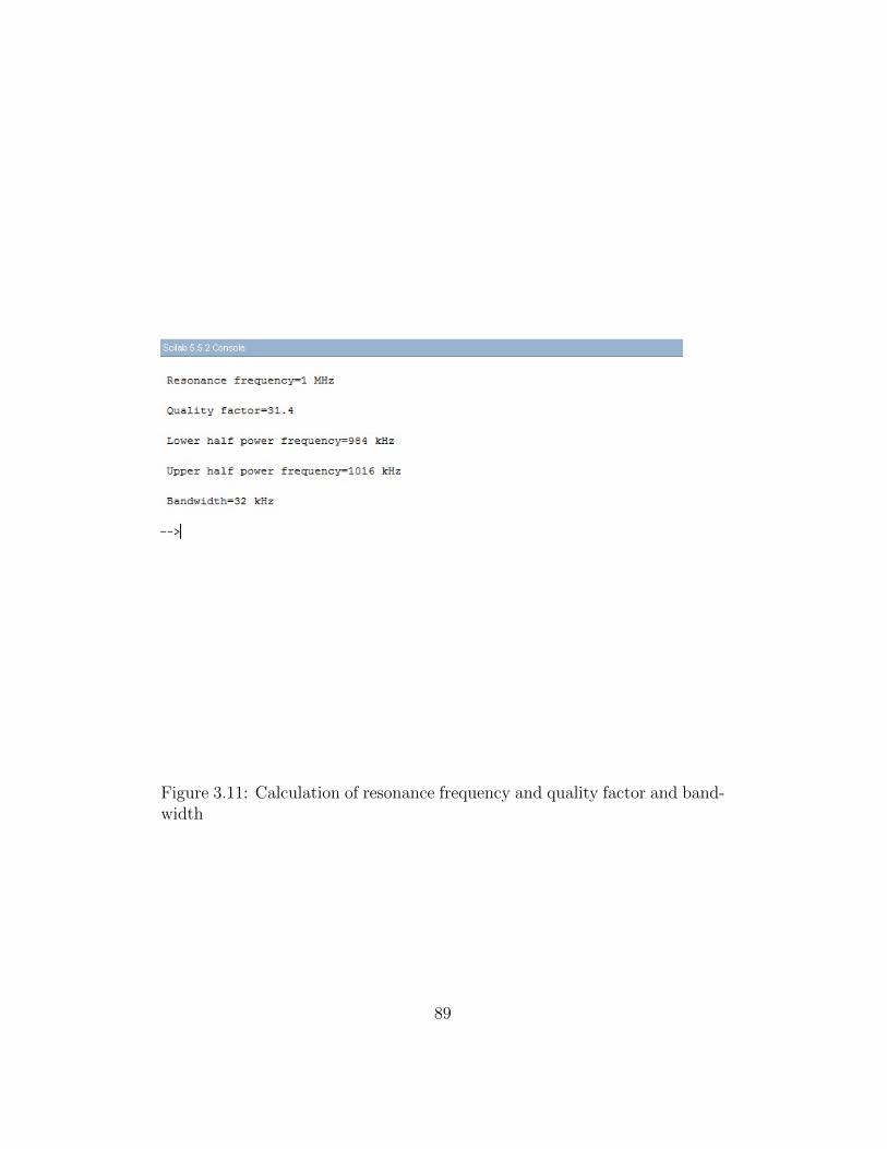
Figure 3.11: Calculation of resonance frequency and quality factor and band-width
89

Scilab code Exa 3.12 Calculation of resonance frequency and quality factor and bandwidth
1 // Book Name : Fundamentals o f E l e c t r i c a l E n g i n e e r i n g2 // Author : Rajendra Prasad3 // P u b l i s h e r : PHI Lea rn ing P r i v a t e L imi ted4 // E d i t i o n : Third ,20145
6 // Ex3 12 . s c e7
8 clc;
9 clear;
10 R=10e3; // R e s i s t a n c e i n ohm11 L=50.7e-6; // I n d u c t o r v a l u e i n henry12 C=500e-12; // c a p a c i t o r v a l u e i n f a r a d13
14 fr =1/(2* %pi*sqrt(L*C));
15 printf(”\n Resonance f r e q u e n c y=%1 . 0 f MHz \n”,fr*1e-6)
16
17 Q=(R)*sqrt(C/L);
18 printf(”\n Qua l i t y f a c t o r=%2 . 1 f \n”,Q)19
20 f1=(-fr/(2*Q))+(fr*sqrt ((1/(2*Q))^2+1));
21 printf(”\n Lower h a l f power f r e q u e n c y=%3 . 0 f kHz \n”,f1*1e-3)
22
23 f2=(fr/(2*Q))+(fr*sqrt ((1/(2*Q))^2+1));
24 printf(”\n Upper h a l f power f r e q u e n c y=%4 . 0 f kHz \n”,f2*1e-3)
25
26 BW=f2-f1;
27 printf(”\n Bandwidth=%2 . 0 f kHz \n”,BW*1e-3)
90
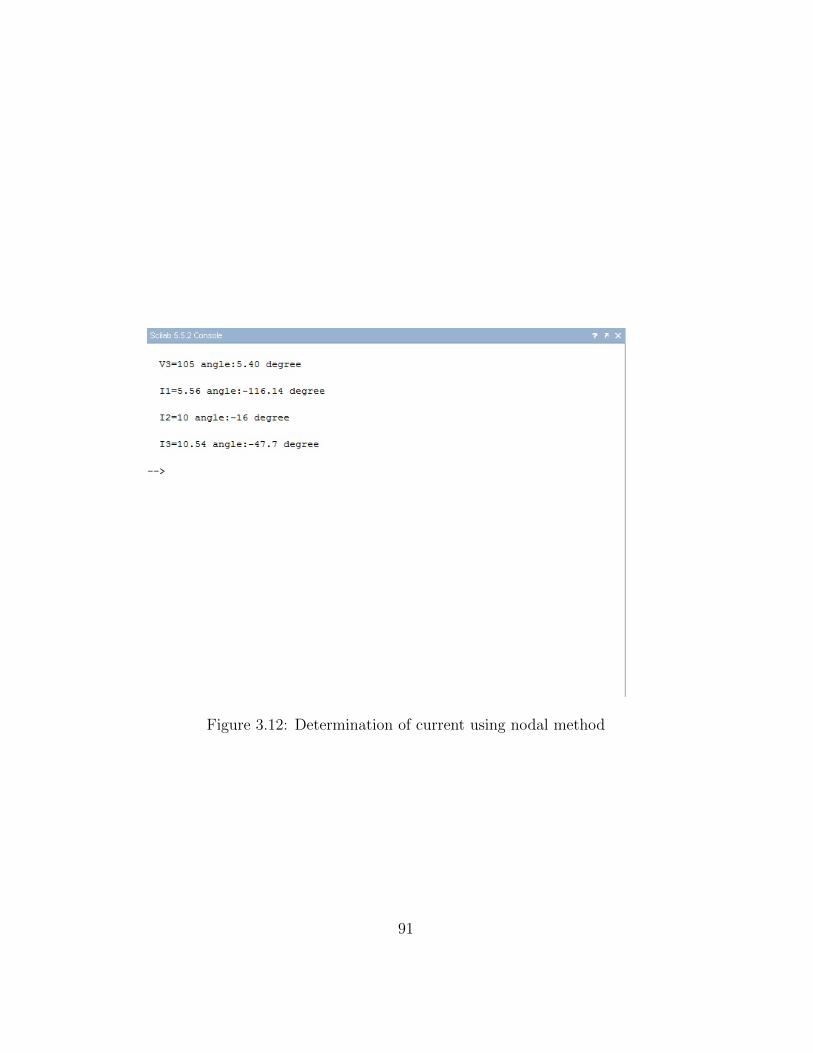
Figure 3.12: Determination of current using nodal method
91

Scilab code Exa 3.13 Determination of current using nodal method
1 // Book Name : Fundamentals o f E l e c t r i c a l E n g i n e e r i n g2 // Author : Rajendra Prasad3 // P u b l i s h e r : PHI Lea rn ing P r i v a t e L imi ted4 // E d i t i o n : Third ,20145
6 // Ex3 13 . s c e7
8 clc;
9 clear;
10
11 // from the f i g u r e 3 . 2 5 the below v a l u e s a r e taken12 Z1=complex (1.2 ,1.6);
13 Z2=complex (1.0 , -1.75);
14 Z12=complex (6,8);
15
16 V1=complex (110 ,0);
17 V2=complex (110* cosd(-5) ,110* sind(-5));
18
19 //VA i s c a l c u l a t e d from the noda l e q u a t i o n o f node A20 VA=((V1/Z1)+(V2/Z2))/(1/Z1 + 1/Z2 + 1/Z12);
21 VA_mag=sqrt(real(VA)^2+ imag(VA)^2);
22 VA_ang=atand(imag(VA)/real(VA));
23 printf(”\n V3=%3 . 0 f a n g l e : %1 . 2 f d e g r e e \n”,VA_mag ,VA_ang)
24
25 I1=(V1-VA)/Z1;
26 I1_mag=sqrt(real(I1)^2+ imag(I1)^2);
27 I1_ang=atand(imag(I1)/real(I1)) -180;
28 printf(”\n I1=%1 . 2 f a n g l e : %3 . 2 f d e g r e e \n”,I1_mag ,I1_ang)
29
30 I2=(V2-VA)/Z2;
31 I2_mag=sqrt(real(I2)^2+ imag(I2)^2);
32 I2_ang=atand(imag(I2)/real(I2));
33 printf(”\n I2=%2 . 0 f a n g l e : %2 . 0 f d e g r e e \n”,I2_mag ,I2_ang)
92
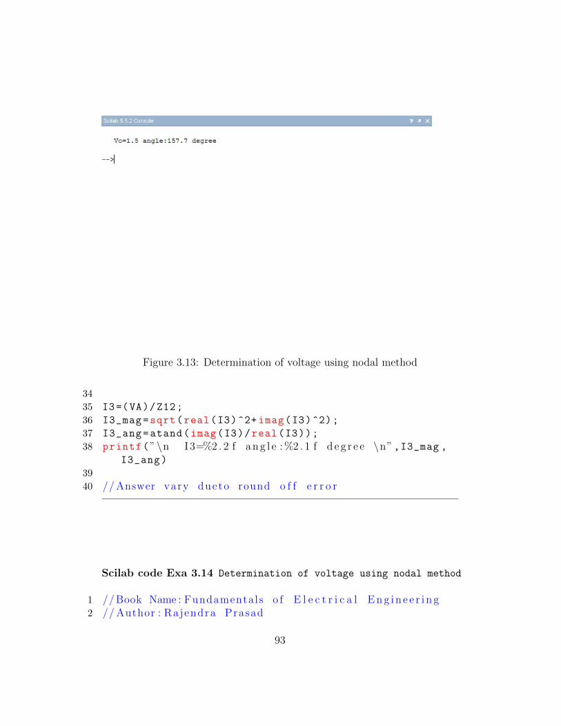
Figure 3.13: Determination of voltage using nodal method
34
35 I3=(VA)/Z12;
36 I3_mag=sqrt(real(I3)^2+ imag(I3)^2);
37 I3_ang=atand(imag(I3)/real(I3));
38 printf(”\n I3=%2 . 2 f a n g l e : %2 . 1 f d e g r e e \n”,I3_mag ,I3_ang)
39
40 // Answer vary dueto round o f f e r r o r
Scilab code Exa 3.14 Determination of voltage using nodal method
1 // Book Name : Fundamentals o f E l e c t r i c a l E n g i n e e r i n g2 // Author : Rajendra Prasad
93

3 // P u b l i s h e r : PHI Lea rn ing P r i v a t e L imi ted4 // E d i t i o n : Third ,20145
6 // Ex3 14 . s c e7
8 clc;
9 clear;
10
11 // i ( t )=s q r t ( 2 ) ∗1 e−4∗ co s (4∗10ˆ7∗ t ) ;12 a1=complex (5 ,4.04);b1=complex (0, -0.04);c1 =1/10;
// t h e s e a r e thec o e f f i c i e n t v a l u e s o f VA,VB and s o u r c e o b t a i n e dfrom the node A i n the g i v e n c i r c u i t
13 a2=complex (200 , -0.04);b2=complex (1.2 , -1.56);c2=0;
// t h e s e a r e thec o e f f i c i e n t v a l u e s o f VA,VB and s o u r c e o b t a i n e dfrom the node B i n the g i v e n c i r c u i t
14 del=det([a1 b1;a2 b2]);
15 delB=det([a1 c1;a2 c2]);
16 VB=delB/del;
17
18 VB_mag=sqrt(real(VB)^2+ imag(VB)^2);
19 VB_ang=atand(imag(VB)/real(VB))+180;
20 printf(”\n Vo=%1 . 1 f a n g l e : %3 . 1 f d e g r e e \n”,VB_mag ,VB_ang)
21
22 // Answer vary due to r o u n d o f f e r r o r23 // R e s u l t : Vo( t )=s q r t ( 2 ) ∗1 . 5∗ co s (4∗10ˆ7∗ t +157 .7)
Scilab code Exa 3.15 Determination of current using mesh analysis
1 // Book Name : Fundamentals o f E l e c t r i c a l E n g i n e e r i n g2 // Author : Rajendra Prasad
94

Figure 3.14: Determination of current using mesh analysis
3 // P u b l i s h e r : PHI Lea rn ing P r i v a t e L imi ted4 // E d i t i o n : Third ,20145
6 // Ex3 15 . s c e7
8 clc;
9 clear;
10 V1=complex (12,0);
11 // c u r r e n t s o u r c e and i t s p a r a l l e l impedance g i v e sthe v o l t a g e s o u r c e
12 V2=complex (5* cosd (-30) ,5*sind (-30))*complex (6,-3);
13 // f o r l oop1 , the c o e f f i c i e n t o f I 1 , I 2 and s o u r c ei s g i v e n below
14 a1=complex (10+6 ,15);
15 b1=-complex (10 ,15);
16 c1=V1;
17 // f o r l oop2 , the c o e f f i c i e n t o f I 1 , I 2 and s o u r c ei s g i v e n below
18 a2=-complex (10 ,15);
95

Figure 3.15: Determination of voltage using mesh analysis
19 b2=complex (19 ,12);
20 c2=-V2;
21 del2=det([a1 c1;a2 c2]);
22 del=det([a1 b1;a2 b2]);
23 I2=del2/del;
24 I2_mag=sqrt(real(I2)^2+ imag(I2)^2);
25 I2_ang=atand(imag(I2)/real(I2))+180;
26 printf(”\n Current through the 3 ohm r e s i s t o r=%1 . 3 fa n g l e : %3 . 2 f d e g r e e \n”,I2_mag ,I2_ang)
Scilab code Exa 3.16 Determination of voltage using mesh analysis
1 // Book Name : Fundamentals o f E l e c t r i c a l E n g i n e e r i n g2 // Author : Rajendra Prasad
96
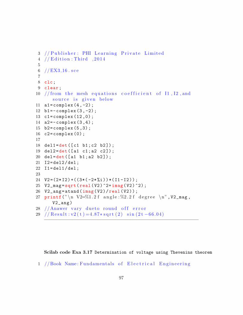
3 // P u b l i s h e r : PHI Lea rn ing P r i v a t e L imi ted4 // E d i t i o n : Third ,20145
6 // EX3 16 . s c e7
8 clc;
9 clear;
10 // from the mesh e q u a t i o n s c o e f f i c i e n t o f I1 , I2 , ands o u r c e i s g i v e n below
11 a1=complex (4,-2);
12 b1=-complex (3,-2);
13 c1=complex (12,0);
14 a2=-complex (3,4);
15 b2=complex (5,3);
16 c2=complex (0);
17
18 del1=det([c1 b1;c2 b2]);
19 del2=det([a1 c1;a2 c2]);
20 del=det([a1 b1;a2 b2]);
21 I2=del2/del;
22 I1=del1/del;
23
24 V2=(2*I2)+((3*( -2*%i))*(I1-I2));
25 V2_mag=sqrt(real(V2)^2+ imag(V2)^2);
26 V2_ang=atand(imag(V2)/real(V2));
27 printf(”\n V2=%1 . 2 f a n g l e : %2 . 2 f d e g r e e \n”,V2_mag ,V2_ang)
28 // Anawer vary dueto round o f f e r r o r29 // R e s u l t : v2 ( t ) =4.87∗ s q r t ( 2 ) s i n (2 t −66 .04)
Scilab code Exa 3.17 Determination of voltage using Thevenins theorem
1 // Book Name : Fundamentals o f E l e c t r i c a l E n g i n e e r i n g
97

Figure 3.16: Determination of voltage using Thevenins theorem
2 // Author : Rajendra Prasad3 // P u b l i s h e r : PHI Lea rn ing P r i v a t e L imi ted4 // E d i t i o n : Third ,20145
6 // Ex3 17 . s c e7
8 clc;
9 clear;
10 // Below v a l u e s a r e taken from the g i v e n c i r c u i t ( f i g. 3 . 2 9 )
11 Z1=complex (5,-5);
12 Z2=complex (5,-5);
13 Z3=complex (10 ,10);
14 V=complex (100 ,0);
15
16 I=V/(Z1+Z2);
17 Vab=I*Z2;
18 Zs=(Z1*Z2)/(Z1+Z2)+Z3;
98
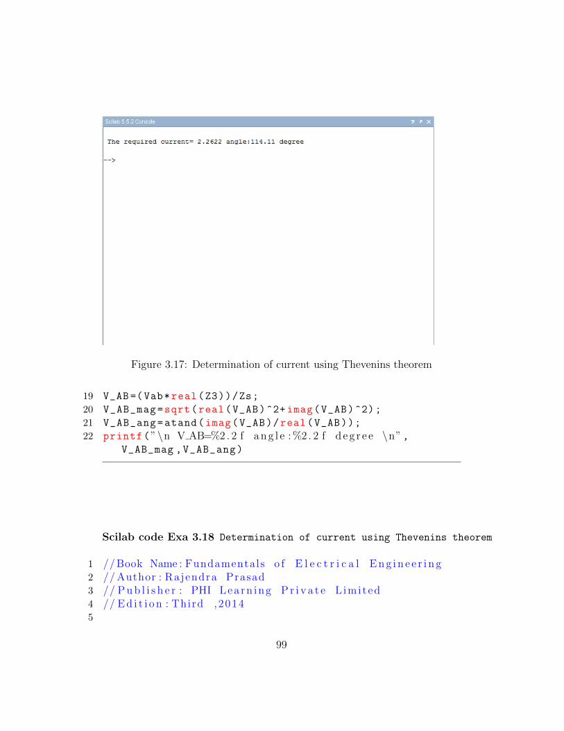
Figure 3.17: Determination of current using Thevenins theorem
19 V_AB=(Vab*real(Z3))/Zs;
20 V_AB_mag=sqrt(real(V_AB)^2+ imag(V_AB)^2);
21 V_AB_ang=atand(imag(V_AB)/real(V_AB));
22 printf(”\n V AB=%2. 2 f a n g l e : %2 . 2 f d e g r e e \n”,V_AB_mag ,V_AB_ang)
Scilab code Exa 3.18 Determination of current using Thevenins theorem
1 // Book Name : Fundamentals o f E l e c t r i c a l E n g i n e e r i n g2 // Author : Rajendra Prasad3 // P u b l i s h e r : PHI Lea rn ing P r i v a t e L imi ted4 // E d i t i o n : Third ,20145
99

6 // Ex3 18 . s c e7
8 clc;
9 clear;
10 // Below v a l u e s a r e taken from the g i v e n c i r c u i t ( f i g. 3 . 2 7 )
11 Z1=complex (6,0);
12 Z2=complex (10 ,15);
13 Z3=complex (6,-3);
14
15 Zs=(Z1*Z2)/(Z1+Z2)+Z3;
16 V=12;
17 Va=V-(V/(Z1+Z2))*real(Z3);
18 Is=complex (5* cosd (-30) ,5*sind (-30));
19 Vb=Is*Z3;
20 Voc=Va -Vb;
21 I=Voc/(Zs+3);
22 I_mag=sqrt(real(I)^2+ imag(I)^2);
23 I_ang=atand(imag(I)/real(I))+180;
24 printf(”\n The r e q u i r e d c u r r e n t= %1 . 4 f a n g l e : %3 . 2 fd e g r e e \n”,I_mag ,I_ang)
Scilab code Exa 3.19 Determination of current using Norton theorem
1 // Book Name : Fundamentals o f E l e c t r i c a l E n g i n e e r i n g2 // Author : Rajendra Prasad3 // P u b l i s h e r : PHI Lea rn ing P r i v a t e L imi ted4 // E d i t i o n : Third ,20145
6 // Ex3 19 . s c e7
8 clc;
9 clear;
100
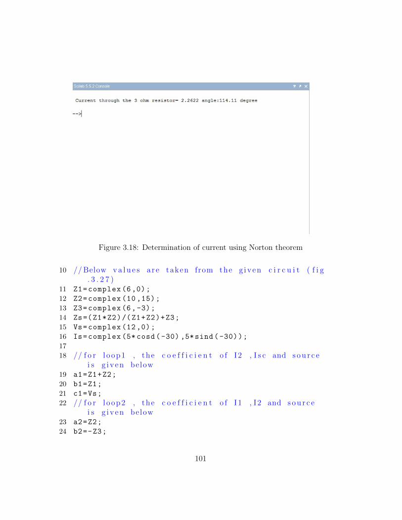
Figure 3.18: Determination of current using Norton theorem
10 // Below v a l u e s a r e taken from the g i v e n c i r c u i t ( f i g. 3 . 2 7 )
11 Z1=complex (6,0);
12 Z2=complex (10 ,15);
13 Z3=complex (6,-3);
14 Zs=(Z1*Z2)/(Z1+Z2)+Z3;
15 Vs=complex (12,0);
16 Is=complex (5* cosd (-30) ,5*sind (-30));
17
18 // f o r l oop1 , the c o e f f i c i e n t o f I 2 , I s c and s o u r c ei s g i v e n below
19 a1=Z1+Z2;
20 b1=Z1;
21 c1=Vs;
22 // f o r l oop2 , the c o e f f i c i e n t o f I 1 , I 2 and s o u r c ei s g i v e n below
23 a2=Z2;
24 b2=-Z3;
101

Figure 3.19: Calculation of impedence and maximum power
25 c2=Is*Z3;
26 del2=det([a1 c1;a2 c2]);
27 del=det([a1 b1;a2 b2]);
28
29 Isc=del2/del;
30 Ys=1/Zs;
31 I=(Isc/Ys)/((1/ Ys)+3);
32 I_mag=sqrt(real(I)^2+ imag(I)^2);
33 I_ang=atand(imag(I)/real(I))+180;
34 printf(”\n Current through the 3 ohm r e s i s t o r= %1 . 4 fa n g l e : %3 . 2 f d e g r e e \n”,I_mag ,I_ang)
102
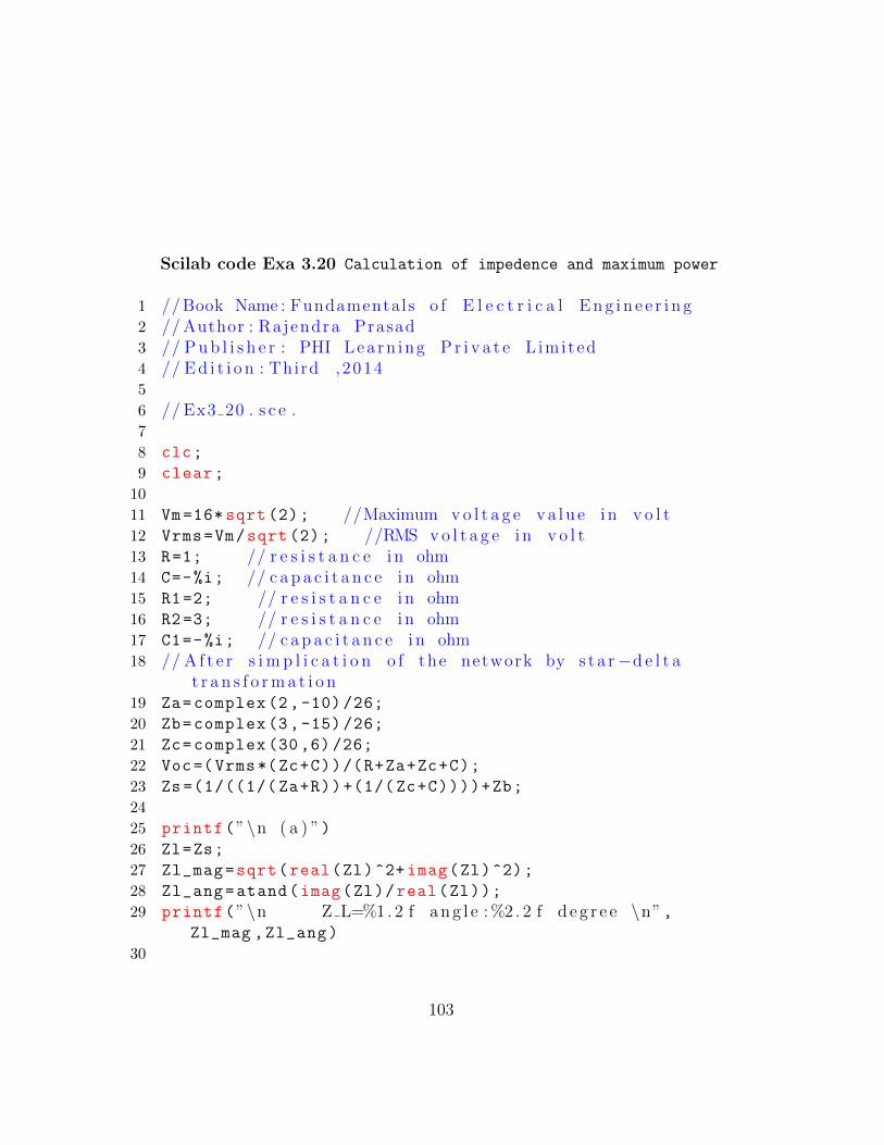
Scilab code Exa 3.20 Calculation of impedence and maximum power
1 // Book Name : Fundamentals o f E l e c t r i c a l E n g i n e e r i n g2 // Author : Rajendra Prasad3 // P u b l i s h e r : PHI Lea rn ing P r i v a t e L imi ted4 // E d i t i o n : Third ,20145
6 // Ex3 20 . s c e .7
8 clc;
9 clear;
10
11 Vm=16* sqrt (2); //Maximum v o l t a g e v a l u e i n v o l t12 Vrms=Vm/sqrt (2); //RMS v o l t a g e i n v o l t13 R=1; // r e s i s t a n c e i n ohm14 C=-%i; // c a p a c i t a n c e i n ohm15 R1=2; // r e s i s t a n c e i n ohm16 R2=3; // r e s i s t a n c e i n ohm17 C1=-%i; // c a p a c i t a n c e i n ohm18 // A f t e r s i m p l i c a t i o n o f the network by s t a r−d e l t a
t r a n s f o r m a t i o n19 Za=complex (2,-10)/26;
20 Zb=complex (3,-15)/26;
21 Zc=complex (30,6) /26;
22 Voc=(Vrms*(Zc+C))/(R+Za+Zc+C);
23 Zs =(1/((1/( Za+R))+(1/(Zc+C))))+Zb;
24
25 printf(”\n ( a ) ”)26 Zl=Zs;
27 Zl_mag=sqrt(real(Zl)^2+ imag(Zl)^2);
28 Zl_ang=atand(imag(Zl)/real(Zl));
29 printf(”\n Z L=%1 . 2 f a n g l e : %2 . 2 f d e g r e e \n”,Zl_mag ,Zl_ang)
30
103

Figure 3.20: Determination of voltage and power and reactive power
31 printf(”\n ( b ) ”)32 Voc_mag=sqrt(real(Voc)^2+ imag(Voc)^2);
33 Pmax=Voc_mag ^2/(2* real(Zl));
34 printf(”\n Maximum power=%2 . 2 f watt \n”,Pmax)35 // There i s a mi s take i n Zs c a l c u l a t i o n . Zs
=0.7555−0.8539 i i s wrong . the c o r r e c t v a l u e o fZs =0.6829−0.8536 i
36 // So the answer vary
Scilab code Exa 3.21 Determination of voltage and power and reactive power
1 // Book Name : Fundamentals o f E l e c t r i c a l E n g i n e e r i n g2 // Author : Rajendra Prasad3 // P u b l i s h e r : PHI Lea rn ing P r i v a t e L imi ted
104

4 // E d i t i o n : Third ,20145
6 // Ex3 21 . s c e7
8 clc;
9 clear;
10 P1=7e3; // s u p p l i e d power i n watt11 pf1 =0.8; // l a g g i n g power f a c t o r12 // below v a l u e s a r e taken from the g i v e n c i r c u i t ( f i g
. 3 . 3 9 )13 Z1=complex (0.8 ,1);
14 Z2=complex (1.4 ,1.6);
15 V1=440; // t e r m i n a l v o l t a g e i n v o l t16 PL=10e3; // power r e q u i r e d by the l oad i n watt17 pf2 =0.8; // l a g g i n g power f a c t o r18
19 I1=P1/(V1*pf1);
20 Pr1=P1 -(I1^2* real(Z1));
21 Q1=P1*tand(acosd(pf1));
22 Qr1=Q1 -(I1^2* imag(Z1));
23 VA=sqrt(Pr1 ^2+Qr1^2);
24 VL=VA/I1;
25 printf(”\n V L=%3 . 1 f V \n”,VL)26
27 QL=PL*tand(acosd(pf2));
28 Pr2=PL -Pr1;
29 Qr2=QL -Qr1;
30 VA_load=sqrt(Pr2 ^2+Qr2^2);
31 I2=VA_load/VL;
32
33 P2=Pr2+(I2^2* real(Z2));
34 Q2=Qr2+(I2^2* imag(Z2));
35 V2=sqrt(P2^2+Q2^2)/I2;
36 printf(”\n V2=%3 . 1 f V \n”,V2)37 printf(”\n R e a c t i v e power : P2=%4 . 1 f W \ t Q2=%4 . 1 f Var
\n”,P2 ,Q2)
105

Figure 3.21: Determination of capacitance and current of alternator
Scilab code Exa 3.22 Determination of capacitance and current of alternator
1 // Book Name : Fundamentals o f E l e c t r i c a l E n g i n e e r i n g2 // Author : Rajendra Prasad3 // P u b l i s h e r : PHI Lea rn ing P r i v a t e L imi ted4 // E d i t i o n : Third ,20145
6 // Ex3 22 . s c e .7
8 clc;
9 clear;
10 V=230; // Supply v o l t a g e i n v o l t11 PL1 =10E3; // supp ly power to l oaad 1 i n watt12 pf1 =0.7; // l a g g i n g power f a c t o r v a l u e o f l o ad 1
106

13 P2=10E3; // supp ly power to l oad 2 i n watt14 pf2 =0.5; // l a g g i n g power f a c t o r v a l u e o f l o ad 215
16 printf(”\n ( a ) ”)17 PL2=P2*pf2;
18 QL1=PL1*tand(acosd(pf1));
19 QL2=PL2*tand(acosd(pf2));
20 PL=PL1+PL2;
21 QL=QL1+QL2;
22 QC=-QL;
23 IC=QC/V;
24 XC=QC/IC^2;
25 f=50;
26 C=1/(2* %pi*f*-XC);
27 printf(”\n The v a l u e o f c a p a c i t a n c e=%4 . 1 f micro−f a r a d \n”,C*1e6)
28
29 printf(”\n ( b ) \ t ( i ) ”)30 kVA=sqrt(PL^2+QL^2);
31 Ig=kVA/V;
32 printf(”\n Magnitude a l t e r n a t o r c u r r e n t wi thoutc a p a c i t o r=%3 . 1 f A \n”,Ig)
33 printf(”\n\ t ( i i ) ”)34 kVA=PL;
35 Ig=kVA/V;
36 printf(”\n Magnitude a l t e r n a t o r c u r r e n t withc a p a c i t o r=%2 . 1 f A \n”,Ig)
37 // Answer vary dueto r o u n d o f f e r r o r
Scilab code Exa 3.27 Plotting the four components from the given circuit
1 // Book Name : Fundamentals o f E l e c t r i c a l E n g i n e e r i n g2 // Author : Rajendra Prasad
107

Figure 3.22: Plotting the four components from the given circuit
3 // P u b l i s h e r : PHI Lea rn ing P r i v a t e L imi ted4 // E d i t i o n : Third ,20145
6 // Ex3 27 ( b ) . s c e7
8 clc;
9 clear;
10 // c a s e ( b )11 // from c a s e ( a ) r e s u l t v ( t ) =5+6.36 s i n ( t ) +2.12 s i n (3 t
) +1.27 s i n (5 t )12 V0=5
13 V1 =6.36/ sqrt (2);
14 V3 =2.12/ sqrt (2);
15 V5 =1.27/ sqrt (2);
16
17 omega0 =0;
18 omega1 =1;
19 omega3 =3;
20 omega5 =5;
21
22 Vdc =(2*V0)/(2+%i*omega0);
23 V1=(2*V1)/(2+%i*omega1)
108
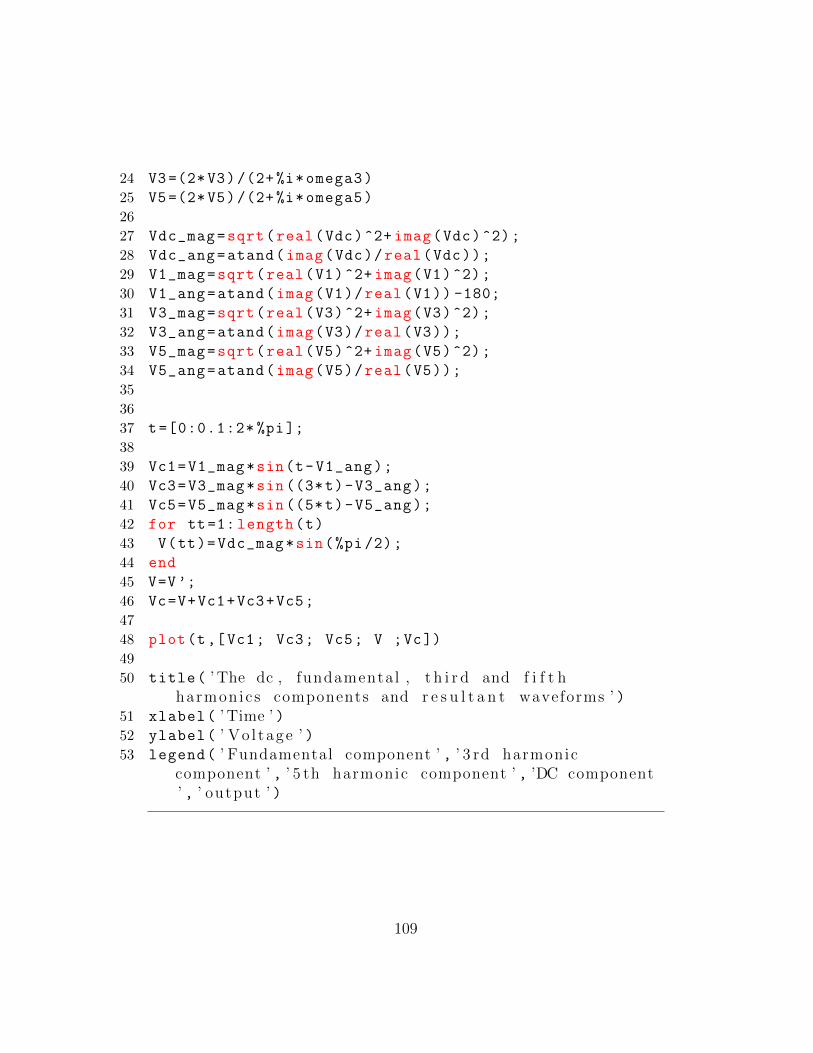
24 V3=(2*V3)/(2+%i*omega3)
25 V5=(2*V5)/(2+%i*omega5)
26
27 Vdc_mag=sqrt(real(Vdc)^2+ imag(Vdc)^2);
28 Vdc_ang=atand(imag(Vdc)/real(Vdc));
29 V1_mag=sqrt(real(V1)^2+ imag(V1)^2);
30 V1_ang=atand(imag(V1)/real(V1)) -180;
31 V3_mag=sqrt(real(V3)^2+ imag(V3)^2);
32 V3_ang=atand(imag(V3)/real(V3));
33 V5_mag=sqrt(real(V5)^2+ imag(V5)^2);
34 V5_ang=atand(imag(V5)/real(V5));
35
36
37 t=[0:0.1:2* %pi];
38
39 Vc1=V1_mag*sin(t-V1_ang);
40 Vc3=V3_mag*sin ((3*t)-V3_ang);
41 Vc5=V5_mag*sin ((5*t)-V5_ang);
42 for tt=1: length(t)
43 V(tt)=Vdc_mag*sin(%pi /2);
44 end
45 V=V’;
46 Vc=V+Vc1+Vc3+Vc5;
47
48 plot(t,[Vc1; Vc3; Vc5; V ;Vc])
49
50 title( ’ The dc , fundamental , t h i r d and f i f t hharmonics components and r e s u l t a n t waveforms ’ )
51 xlabel( ’ Time ’ )52 ylabel( ’ Vo l tage ’ )53 legend( ’ Fundamental component ’ , ’ 3 rd harmonic
component ’ , ’ 5 th harmonic component ’ , ’DC component’ , ’ output ’ )
109

Chapter 4
Electrostatics
Scilab code Exa 4.1 Determination of force between two spheres
1 // Book Name : Fundamentals o f E l e c t r i c a l E n g i n e e r i n g2 // Author : Rajendra Prasad3 // P u b l i s h e r : PHI Lea rn ing P r i v a t e L imi ted4 // E d i t i o n : Third ,20145
6 // Ex4 1 . s c e .7
8 clc;
9 clear;
10 Q1=2e-9; // Sphere 1 c h a r g e s i n coulomb11 Q2=-0.5e-9; // Sphere 2 c h a r g e s i n coulomb12 r=4e-2; // D i s t a n c e between the two s p h e r e s i n m13 epsilon_not =1/(36 e9*%pi);
14 printf(”\n ( a ) ”)15 F=-(Q1*Q2)/(4* %pi*epsilon_not*r^2);
// Coulomb ’ s law16 printf(”\n Force between two s p h e r e s when they a r e
d i s p l a c e d 4cm apar t=%1 . 4 f ∗10ˆ−5 N A t t r a c t i v e \n”,F*1e5)
110

Figure 4.1: Determination of force between two spheres
17
18 printf(”\n ( b ) ”)19 q=(Q1+Q2)/2;
20 F=(q^2) /(4* %pi*epsilon_not*r^2)
21 printf(”\n Force between two s p h e r e s i f they a r ebrought i n t o c o n t a c t and s e p a r a t e d by 4cm =%1 . 4 f∗10ˆ−5 N r e p u l s i v e \n”,F*1e5)
Scilab code Exa 4.3 Calculation of force
1 // Book Name : Fundamentals o f E l e c t r i c a l E n g i n e e r i n g2 // Author : Rajendra Prasad3 // P u b l i s h e r : PHI Lea rn ing P r i v a t e L imi ted4 // E d i t i o n : Third ,20145
6 // Ex4 3 . s c e7
8 clc;
9 clear;
111

Figure 4.2: Calculation of force
10 r=[ -0.03 0.01 0.04];
11 r_dash =[0.03 0.08 -0.02];
12 Q1=129e-9;
13 Q2=110e-6;
14 epsilon_not =1/(36* %pi*1e9);
15
16 a=r-r_dash; // r and r d a s h a r e the p o s i t i o n o f twoc h a r g e s
17 b=a.^2;
18 c=b(1,1)+b(1,2)+b(1,3);
19 d=sqrt(c); //b , c , d a r e assumed a l p h a b e t s f o rc a l c u l a t i n g magnitude o f d i f f e r e n c e o f r and r ’
20
21 F=(Q1*Q2)/(4* %pi*epsilon_not*d^2);
22 printf(”\n The f o r c e on Q2=%2 . 1 f N \n”,F)23 Ir=a/d;
24 F1=Ir*F;
25 printf(”\n Force i n t e r m s o f i , j , k v e c t o r c o e f f i c i e n ti s ”)
26 disp(F1)
27
28 // There i s a e r r o r i n the book f o r c a l c u l a t i n g F
112

Figure 4.3: Determination electric field intensity
v a l u e29 // So answer g i v e n i n the book i s wrong
Scilab code Exa 4.4 Determination electric field intensity
1 // Book Name : Fundamentals o f E l e c t r i c a l E n g i n e e r i n g2 // Author : Rajendra Prasad3 // P u b l i s h e r : PHI Lea rn ing P r i v a t e L imi ted4 // E d i t i o n : Third ,20145
6 // Ex4 4 . s c e .7
8 clc;
9 clear;
10 q=1.6e-19;
11 m=9.1e-31;
12 g=9.8;
113
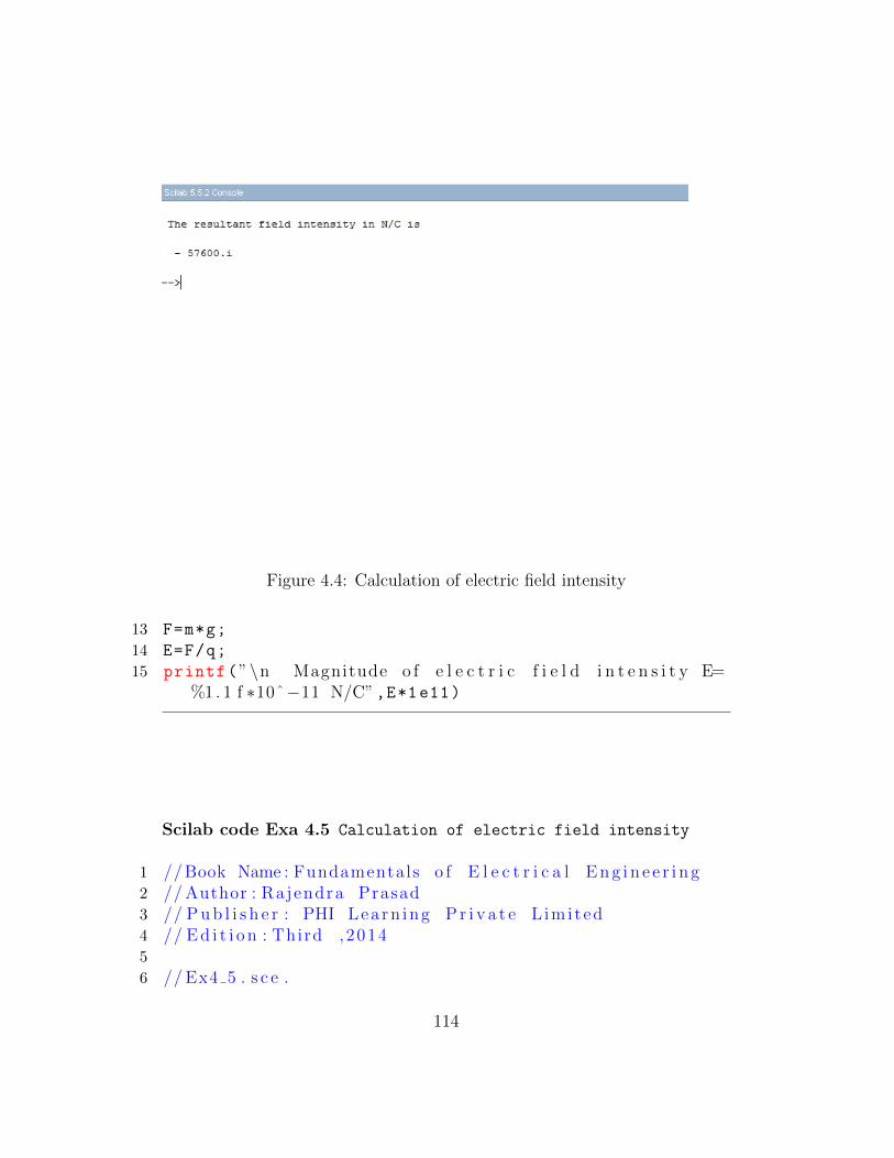
Figure 4.4: Calculation of electric field intensity
13 F=m*g;
14 E=F/q;
15 printf(”\n Magnitude o f e l e c t r i c f i e l d i n t e n s i t y E=%1 . 1 f ∗10ˆ−11 N/C”,E*1e11)
Scilab code Exa 4.5 Calculation of electric field intensity
1 // Book Name : Fundamentals o f E l e c t r i c a l E n g i n e e r i n g2 // Author : Rajendra Prasad3 // P u b l i s h e r : PHI Lea rn ing P r i v a t e L imi ted4 // E d i t i o n : Third ,20145
6 // Ex4 5 . s c e .
114
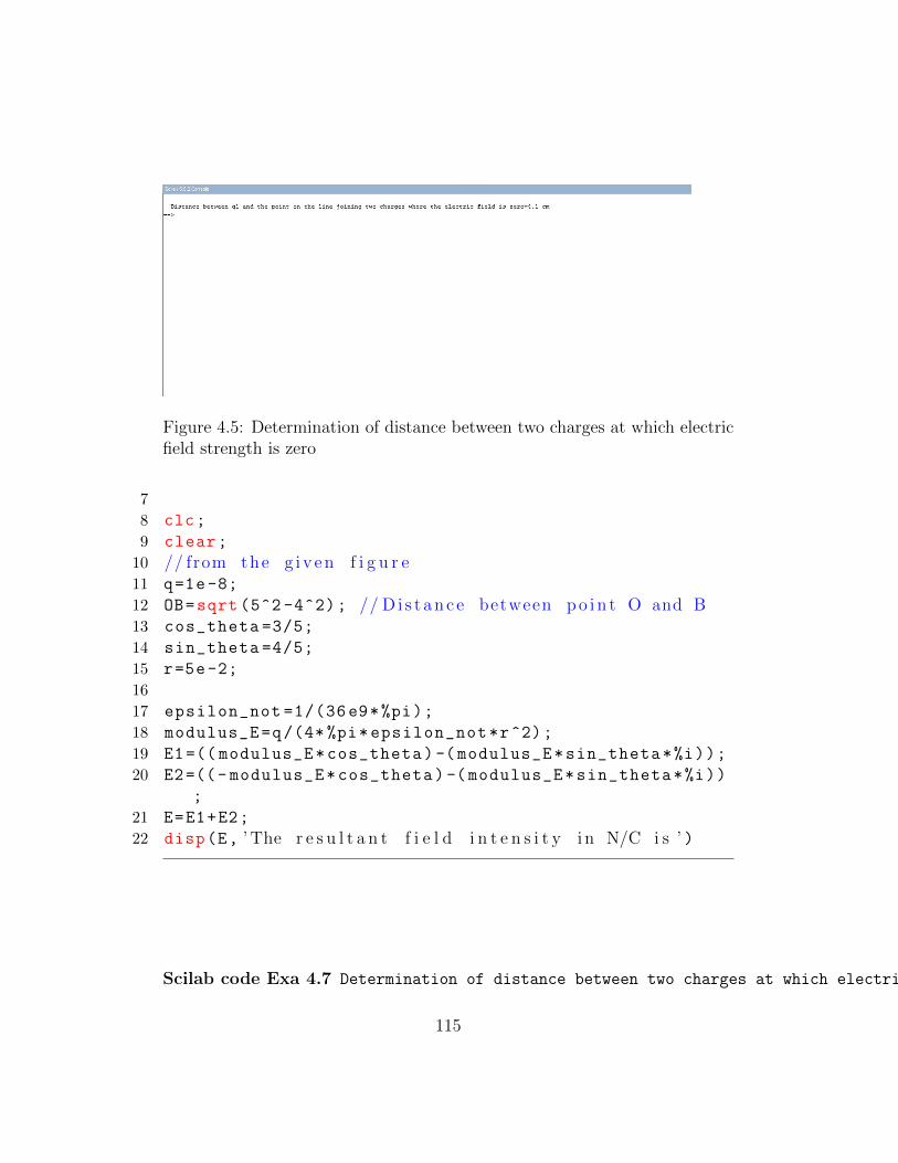
Figure 4.5: Determination of distance between two charges at which electricfield strength is zero
7
8 clc;
9 clear;
10 // from the g i v e n f i g u r e11 q=1e-8;
12 OB=sqrt (5^2 -4^2); // D i s t a n c e between p o i n t O and B13 cos_theta =3/5;
14 sin_theta =4/5;
15 r=5e-2;
16
17 epsilon_not =1/(36 e9*%pi);
18 modulus_E=q/(4* %pi*epsilon_not*r^2);
19 E1=(( modulus_E*cos_theta)-(modulus_E*sin_theta*%i));
20 E2=((- modulus_E*cos_theta) -(modulus_E*sin_theta*%i))
;
21 E=E1+E2;
22 disp(E, ’ The r e s u l t a n t f i e l d i n t e n s i t y i n N/C i s ’ )
Scilab code Exa 4.7 Determination of distance between two charges at which electric field strength is zero
115

Figure 4.6: Determination of maximum torque and work done
1 // Book Name : Fundamentals o f E l e c t r i c a l E n g i n e e r i n g2 // Author : Rajendra Prasad3 // P u b l i s h e r : PHI Lea rn ing P r i v a t e L imi ted4 // E d i t i o n : Third ,20145
6 // Ex4 7 . s c e .7
8 clc;
9 clear;
10 q1=1e-4;
11 q2=2e-4;
12 l=10e-2;
13 x=l*1e2/(1+ sqrt(q2/q1));
14 printf(”\n D i s t a n c e between q1 and the p o i n t on thel i n e j o i n i n g two c h a r g e s where the e l e c t r i c
f i e l d i s z e r o=%1 . 1 f cm”,x)
Scilab code Exa 4.11 Determination of maximum torque and work done
116

1 // Book Name : Fundamentals o f E l e c t r i c a l E n g i n e e r i n g2 // Author : Rajendra Prasad3 // P u b l i s h e r : PHI Lea rn ing P r i v a t e L imi ted4 // E d i t i o n : Third ,20145
6 // Ex4 11 . s c e .7
8 clc;
9 clear;
10 q=1e-6;
11 l=2e-2;
12 E=1e5;
13
14 printf(”\n ( a ) ”)15 theta =90;
16 p=l*q;
17 T_max=p*E*sind(theta);
18 printf(”\n The maximum t o r q u e=%1 . 1 f ∗10ˆ−3 Nm\n”,T_max*1e3)
19
20 printf(”\n ( b ) ”)21 U_180=-p*E*cosd (180); //U i s
the p o t e n t i a l ene rgy f o r t h e t a =180 d e g r e e and 0d e g r e e
22 U_0=-p*E*cosd (0);
23 W=(U_180) -(U_0);
24 printf(”\n The work done=%1 . 1 f ∗10ˆ−3 J”,W*1e3)
Scilab code Exa 4.14 Determination of charge
1 // Book Name : Fundamentals o f E l e c t r i c a l E n g i n e e r i n g2 // Author : Rajendra Prasad3 // P u b l i s h e r : PHI Lea rn ing P r i v a t e L imi ted
117

Figure 4.7: Determination of charge
4 // E d i t i o n : Third ,20145
6 // Ex4 14 . s c e .7
8 clc;
9 clear;
10 V=100;
11 epsilon_not =8.854e-12;
12 r=10e-2;
13 q=4*%pi*epsilon_not*r*V;
14 printf(”\n Magnitude v a l u e o f i s o l a t e d p o s i t i v echa rge=%1 . 2 g∗10ˆ−9 coulomb ”,q*1e9)
Scilab code Exa 4.15 Calculation of potential difference between two points
1 // Book Name : Fundamentals o f E l e c t r i c a l E n g i n e e r i n g2 // Author : Rajendra Prasad3 // P u b l i s h e r : PHI Lea rn ing P r i v a t e L imi ted4 // E d i t i o n : Third ,2014
118
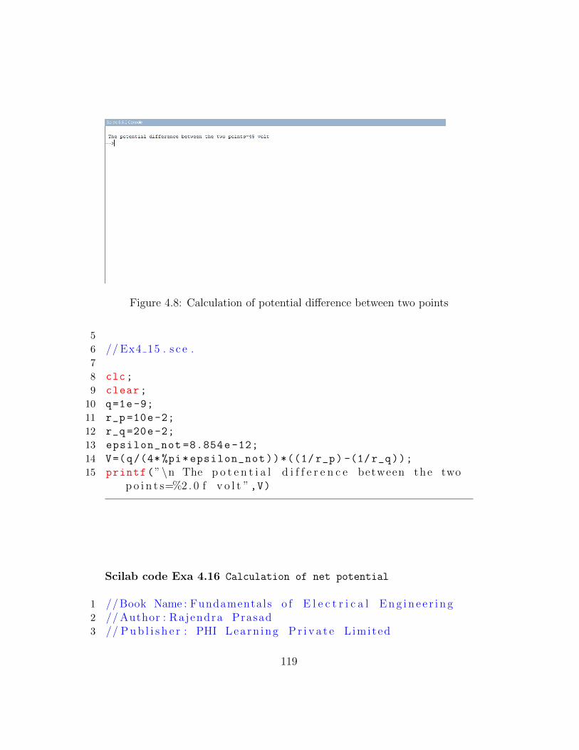
Figure 4.8: Calculation of potential difference between two points
5
6 // Ex4 15 . s c e .7
8 clc;
9 clear;
10 q=1e-9;
11 r_p =10e-2;
12 r_q =20e-2;
13 epsilon_not =8.854e-12;
14 V=(q/(4* %pi*epsilon_not))*((1/ r_p) -(1/r_q));
15 printf(”\n The p o t e n t i a l d i f f e r e n c e between the twop o i n t s=%2 . 0 f v o l t ”,V)
Scilab code Exa 4.16 Calculation of net potential
1 // Book Name : Fundamentals o f E l e c t r i c a l E n g i n e e r i n g2 // Author : Rajendra Prasad3 // P u b l i s h e r : PHI Lea rn ing P r i v a t e L imi ted
119

Figure 4.9: Calculation of net potential
4 // E d i t i o n : Third ,20145
6 // Ex4 16 . s c e .7
8 clc;
9 clear;
10 q1=-2e-9;
11 q2=3e-9;
12 q3=2e-9;
13 q4=1e-9;
14 AB=1; // Given squ a r e s i d e as 1 metre15 BC=1;
16 epsilon_not =8.854e-12;
17 AP=sqrt(AB^2+BC^2) /2; // fo rmu la d e r i v e dfrom the f i g u r e
18 Vp =(1/(4* %pi*epsilon_not*AP))*(q1+q2+q3+q4);
19 printf(”\n P o t e n t i a l a t the c e n t r e o f the sq ua r e=%2. 2 f v o l t ”,Vp)
20
21 // Answer vary due to r o u n d o f f e r r o r
120

Figure 4.10: Calculation of electric field
Scilab code Exa 4.18 Calculation of electric field
1 // Book Name : Fundamentals o f E l e c t r i c a l E n g i n e e r i n g2 // Author : Rajendra Prasad3 // P u b l i s h e r : PHI Lea rn ing P r i v a t e L imi ted4 // E d i t i o n : Third ,20145
6 // Ex4 18 . s c e .7 clc;
8 clear;
9 Q1=3e-6;
10 Q2=2e-6;
11 a=9e9; // a =(1/(4∗%pi∗ e p s i l o n n o t ) )12
13 x=1;y=2;z=3;
14
15 //V=−a ∗ ( ( Q1/( s q r t ( ( x−1)ˆ2+(y−1)ˆ2+(z−1) ˆ2) ) ) +(Q2/(
121

s q r t ( ( x−1)ˆ2+(y−3)ˆ2+(z−2) ˆ2) ) ) ) ;16
17 dV_dx=-a*((Q1*(x-1) /((x-1) ^2+(y-1) ^2+(z-1)^2) ^(3/2))
+(Q2*(x-1) /((x-1) ^2+(y-3) ^2+(z-2)^2) ^(3/2)));
// d i f f e r e n t i e t i o n o f p o t e n t i a l with r e s p e c t to x18
19 dV_dy=-a*((Q1*(y-1) /((x-1) ^2+(y-1) ^2+(z-1)^2) ^(3/2))
+(Q2*(y-3) /((x-1) ^2+(y-3) ^2+(z-2)^2) ^(3/2)));
// d i f f e r e n t i e t i o n o f p o t e n t i a l with r e s p e c t to y20
21 dV_dz=-a*((Q1*(z-1) /((x-1) ^2+(y-1) ^2+(z-1)^2) ^(3/2))
+(Q2*(z-2) /((x-1) ^2+(y-3) ^2+(z-2)^2) ^(3/2)));
// d i f f e r e n t i e t i o n o f p o t e n t i a l with r e s p e c tto z
22
23 //E=−(de l V )24 printf(”\n E=(%gi ) +(%4 . 0 f j ) +(%5 . 0 f k ) V/m”,-dV_dx ,-
dV_dy ,-dV_dz)
Scilab code Exa 4.19 Calculation of potential and field strength
1 // Book Name : Fundamentals o f E l e c t r i c a l E n g i n e e r i n g2 // Author : Rajendra Prasad3 // P u b l i s h e r : PHI Lea rn ing P r i v a t e L imi ted4 // E d i t i o n : Third ,20145
6 // Ex4 19 . s c e .7
8 clc;
9 clear;
10 r1=3e-2;
11 r2=6e-2;
12 r3=9e-2;
122

Figure 4.11: Calculation of potential and field strength
13 q1=9e-12;
14 q2=-6e-12;
15 q3=3e-12;
16 d1=2e-2;
17 d2=4e-2;
18 d3=7e-2;
19 d4=12e-2;
20 epsilon_not =8.854e-12;
21 a=9e9; // a =1/(4∗%pi∗ e p s i l o n n o t ) ;22
23 printf(”\n F i e l d s t r e n g t h and p o t e n t i a l s f o r p o i n t a, b , c , d a r e , ”)
24 Ea=0;
25 printf(”\n\ t Ea=%g N/C”,Ea)26 Va=a*((q1/r1)+(q2/r2)+(q3/r3));
27 printf(”\n\ t Va=%g V \n”,Va)28
29 Eb=a*(q1/d2^2);
30 printf(”\n\ t Eb=%g N/C”,Eb)31 Vb=a*((q1/d2)+(q2/r2)+(q3/r3));
32 printf(”\n\ t Vb=%g V \n”,Vb)
123
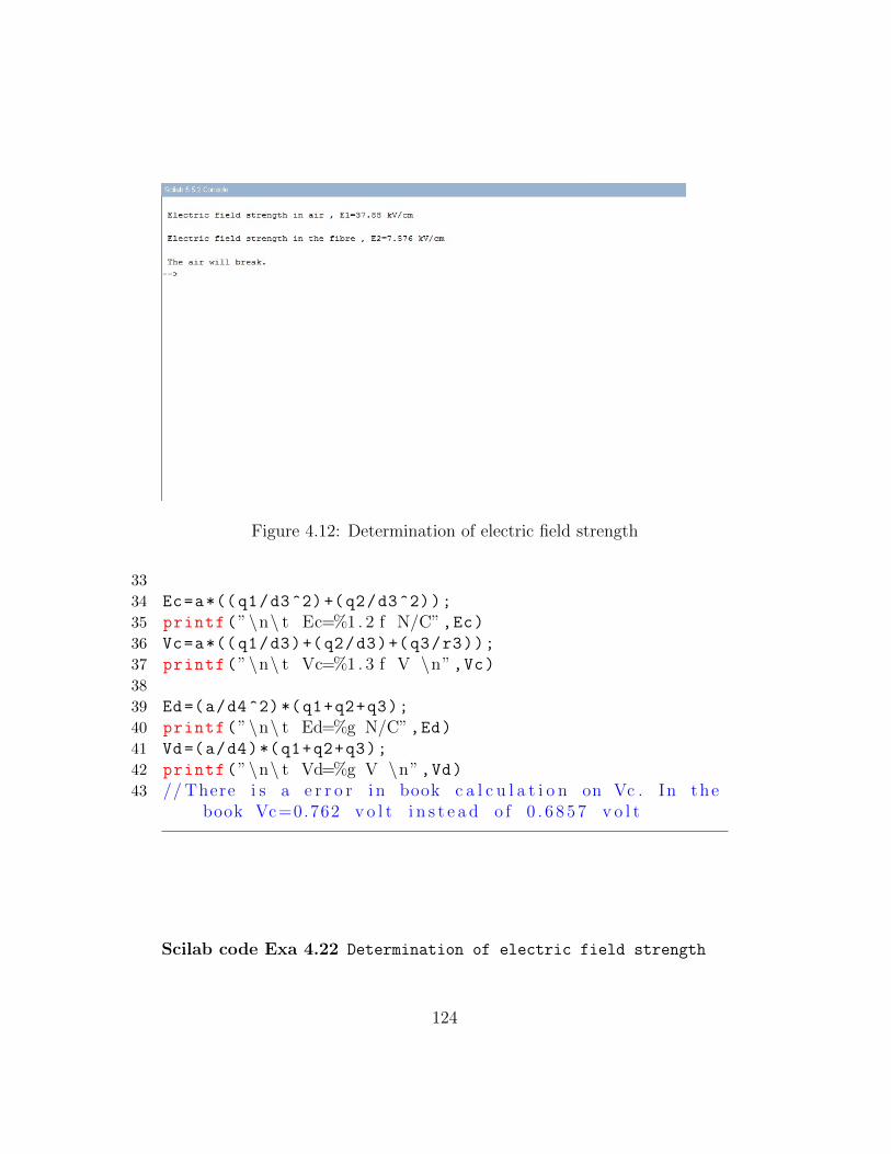
Figure 4.12: Determination of electric field strength
33
34 Ec=a*((q1/d3^2)+(q2/d3^2));
35 printf(”\n\ t Ec=%1 . 2 f N/C”,Ec)36 Vc=a*((q1/d3)+(q2/d3)+(q3/r3));
37 printf(”\n\ t Vc=%1 . 3 f V \n”,Vc)38
39 Ed=(a/d4^2)*(q1+q2+q3);
40 printf(”\n\ t Ed=%g N/C”,Ed)41 Vd=(a/d4)*(q1+q2+q3);
42 printf(”\n\ t Vd=%g V \n”,Vd)43 // There i s a e r r o r i n book c a l c u l a t i o n on Vc . In the
book Vc=0.762 v o l t i n s t e a d o f 0 . 6 8 5 7 v o l t
Scilab code Exa 4.22 Determination of electric field strength
124

1 // Book Name : Fundamentals o f E l e c t r i c a l E n g i n e e r i n g2 // Author : Rajendra Prasad3 // P u b l i s h e r : PHI Lea rn ing P r i v a t e L imi ted4 // E d i t i o n : Third ,20145
6 // Ex4 22 . s c e .7
8 clc;
9 clear;
10 V=2.5; // p o t e n t i a l d i f f e r e n c e o f thep l a t e s i n kv
11 x=0.25; // d i s t a n c e between twop a r a l l e l p l a t e s i n cm
12 x1 =0.02; // a i r g a p i n between thep a r a l l e l p l a t e s i n cm
13 x2 =0.23; // t h i c k n e s s o f f i b r e s h e e t i nthe gap i n cm
14 epsilon_r =5;
15
16 //As the e l e t r i c d i s p l a c e m e n t i s p e r p e n d i c u l a r tothe boundary
17 //D=D1=D2 ; , D1=e p s i l o n n o t ∗E1 ; , D2=e p s i l o n n o t ∗ e p s i l o n r ∗E2 ;
18 // from t h i s E1=5∗E2 ;19
20 //V=V1+V2 ; V1=x1∗E1 ; V2=x2∗E2 ;21 // from t h i s we can f i n d the e q u a t i o n o f E222
23 E2=V/((x1*epsilon_r)+(x2));
24 E1=5*E2;
25
26 printf(”\n E l e c t r i c f i e l d s t r e n g t h i n a i r , E1=%2 . 2 fkV/cm \n”,E1)
27 printf(”\n E l e c t r i c f i e l d s t r e n g t h i n the f i b r e , E2=%1 . 3 f kV/cm \n”,E2)
28
29 E=30; // D i e l e c t r i c s t r e n g t h o f a i r i n kV/cm30 if (E1 >E)
125
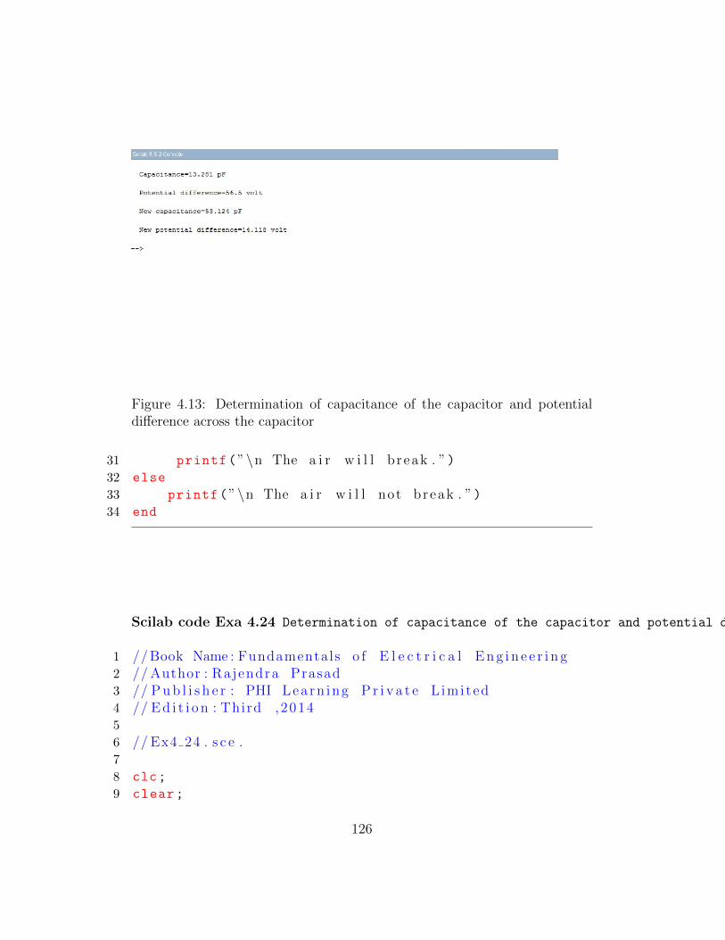
Figure 4.13: Determination of capacitance of the capacitor and potentialdifference across the capacitor
31 printf(”\n The a i r w i l l break . ”)32 else
33 printf(”\n The a i r w i l l not break . ”)34 end
Scilab code Exa 4.24 Determination of capacitance of the capacitor and potential difference across the capacitor
1 // Book Name : Fundamentals o f E l e c t r i c a l E n g i n e e r i n g2 // Author : Rajendra Prasad3 // P u b l i s h e r : PHI Lea rn ing P r i v a t e L imi ted4 // E d i t i o n : Third ,20145
6 // Ex4 24 . s c e .7
8 clc;
9 clear;
126

10 d=1e-2;
11 l=15e-2;
12 h=10e-2;
13 Q=750e-12;
14 epsilon_not =8.854e-12;
15
16 A=l*h;
17 C=( epsilon_not*A)/d;
18 printf(”\n Capac i t ance=%2 . 3 f pF \n”,C*1e12)19 V=Q/C;
20 printf(”\n P o t e n t i a l d i f f e r e n c e=%2 . 1 f v o l t \n”,V)21
22 epsilon_r =4;
23 C=( epsilon_not*epsilon_r*A)/d;
24 printf(”\n New c a p a c i t a n c e=%2 . 3 f pF \n”,C*1e12)25 V=Q/C;
26 printf(”\n New p o t e n t i a l d i f f e r e n c e=%2 . 3 f v o l t \n”,V)
27
28 // There i s a e r r o r i n the book c a l c u l a t i o n f o rf i n d i n g new p o t e n t i a l d i f f e r e n c e (V) , the answeri s g i v e n V=14.125 v o l t i n s t e a d o f 1 4 . 1 1 8 v o l t
Scilab code Exa 4.26 Calculation of electric field intensity and electric flux density
1 // Book Name : Fundamentals o f E l e c t r i c a l E n g i n e e r i n g2 // Author : Rajendra Prasad3 // P u b l i s h e r : PHI Lea rn ing P r i v a t e L imi ted4 // E d i t i o n : Third ,20145
6 // Ex4 26 . s c e .7
8 clc;
127

Figure 4.14: Calculation of electric field intensity and electric flux density
9 clear;
10 d_i=5e-3; // Diameter o f i n n e r c y l i n d e ri n metre
11 d_o =15e-3; // Diameter o f o u t e r c y l i n d e ri n metre
12 epsilon_r =4;
13 V=500;
14 epsilon_not =8.854e-12;
15 epsilon=epsilon_r*epsilon_not;
16 a=d_i/2;
17 b=d_o/2;
18 C=(2* %pi*epsilon)/(log(b/a));
19 printf(”\n Capac i t ance o f the c a b l e=%3 . 2 f pF/m \n”,C*1e12)
20
21 printf(”\n ( a ) ”)22 p_l=C*V; // E l e c t r i c d i s p l a c e m e n t
through a c y l i n d r i c a l a r ea o f u n i t l e n g t h i n C/m23 D=p_l /(2* %pi*a);
24 E=D/epsilon;
25 printf(”\n The e l e c t r i c f l u x d e n s i t y at the s u r f a c e
128

Figure 4.15: Calculation of capacitance of the line
o f i n n e r conduc to r=%1 . 3 f micro C /mˆ2 ”,D*1e6)26 printf(”\n The e l e c t r i c f i e l d i n t e n s i t y at the
s u r f a c e o f i n n e r conduc to r=%3 . 0 f kV/m \n”,E*1e-3)27
28 printf(”\n ( b ) ”)29 D=p_l /(2* %pi*b);
30 E=D/epsilon;
31 printf(”\n The e l e c t r i c f l u x d e n s i t y at the i n n e rs u r f a c e o f o u t e r conduc to r=%1 . 3 f micro C /mˆ2 ”,D*1e6)
32 printf(”\n The e l e c t r i c f i e l d i n t e n s i t y at thei n n e r s u r f a c e o f o u t e r conduc to r=%2 . 3 f kV/m \n”,E*1e-3)
33 // Answer vary dueto round o f f e r r o r
Scilab code Exa 4.27 Calculation of capacitance of the line
1 // Book Name : Fundamentals o f E l e c t r i c a l E n g i n e e r i n g
129
Figure 4.16: Calculation of thickness of the dielectric
2 // Author : Rajendra Prasad3 // P u b l i s h e r : PHI Lea rn ing P r i v a t e L imi ted4 // E d i t i o n : Third ,20145
6 // Ex4 27 . s c e .7
8 clc;
9 clear;
10 l=4e3;
11 b=2*75e-2;
12 a=2.5e-2;
13 epsilon_not =8.854e-12;
14 C=(%pi*epsilon_not*l)/log(b/a);
15 printf(”\n Capac i t ance o f the t r a n s m i s s i o n l i n e=%1 . 4f micro f a r a d ”,C*1e6)
Scilab code Exa 4.28 Calculation of thickness of the dielectric
130

1 // Book Name : Fundamentals o f E l e c t r i c a l E n g i n e e r i n g2 // Author : Rajendra Prasad3 // P u b l i s h e r : PHI Lea rn ing P r i v a t e L imi ted4 // E d i t i o n : Third ,20145
6 // Ex4 28 . s c e .7
8 clc;
9 clear;
10 t1=1.5; // I n s u l a t i o n t h i c k n e s s o fconduc to r i n cm
11 d_c =1.5; // Diameter o f conduc to r i n cm12 a1=d_c/2;
13 b1=a1+t1;
14 R1=500; // I n s u l a t i o n r e s i s t a n c e i nmegaohm f o r a g i v e n t h i c k n e s s
15 R2=700; // I n s u l a t i o n r e s i s t a n c e i nmegaohm f o r a unknown t h i c k n e s s
16
17 //R=(p /(2∗%pi∗ l ) ) ∗ l o g ( b/a ) R1=(p /(2∗%pi∗ l ) ) ∗l o g ( b1/ a1 ) R2=(p /(2∗%pi∗ l ) ) ∗ l o g ( b2/a2 )
18
19 a2=d_c/2;
20 b2=a2; // b2 i s the sum o f a2 and unknownt h i c k n e s s
21
22 t2=a2*(b1/a1)^(R2/R1)-b2; // t h i c k n e s s o f 700megaohm r e s i s t a n c e i n s u l a t i o n i n cm
23 printf(”\n I n s u l a t i o n t h i c k n e s s o f the c a b l e i fi n s u l a t i o n r e s i s t a n c e i s 700 megaohm=%1 . 3 f cm”,t2)
131
Figure 4.17: Determination of loss energy
Scilab code Exa 4.29 Determination of loss energy
1 // Book Name : Fundamentals o f E l e c t r i c a l E n g i n e e r i n g2 // Author : Rajendra Prasad3 // P u b l i s h e r : PHI Lea rn ing P r i v a t e L imi ted4 // E d i t i o n : Third ,20145
6 // Ex4 29 . s c e .7
8 clc;
9 clear;
10 Q1=60e-6; // C a p a c i t o r c h a r g e s i n coulomb11 V1=180; // Vo la tge i n v o l t12
13 C1=Q1/V1;
14 C2=4*C1;
15 Q2=0;
16 E1 =(1/2)*C1*V1^2; // B e f o r e two
132

c a p a c i t a n c e a r e j o i n e d the ene rgy s t o r e d i n C117 E2=0; // Energy s t o r e d i n C218 Ea=E1+E2; // Tota l ene rgy b e f o r e
two c a p a c i t o r s a r e j o i n e d19 V=(Q1+Q2)/(C1+C2); // P o t e n t i a l i n v o l t20
21 E1 =(1/2)*C1*V^2; // Energy s t o r e d i n C1 i nj o u l e
22 E2 =(1/2)*C2*V^2; // Energy s t o r e d i n C2 i nj o u l e
23 Eb=E1+E2; // Tota l ene rgy a f t e r twoc a p a c i t o r s a r e j o i n e d
24
25 E_loss=Ea-Eb;
26 printf(”\n Loss o f ene rgy=%2 . 1 f ∗10ˆ−4 j o u l e ”,E_loss*1e4)
133
Chapter 5
Electromagnetism andElectromechanical EnergyConversion
Scilab code Exa 5.5 Determination of mmf and total flux and flux density
1 // Book Name : Fundamentals o f E l e c t r i c a l E n g i n e e r i n g2 // Author : Rajendra Prasad3 // P u b l i s h e r : PHI Lea rn ing P r i v a t e L imi ted4 // E d i t i o n : Third ,20145
6 // Ex5 5 . s c e .7
8 clc;
9 clear;
10 N=200;
11 A=5e-4;
12 I=4;
13 l=60e-2;
14
15 printf(”\n\ t ( a ) ”)
134

Figure 5.1: Determination of mmf and total flux and flux density
16 F=N*I;
17 printf(”\n Magnetomotive f o r c e=%d AT \n”,F)18
19 printf(”\n\ t ( b ) ”)20 mew_r =1;
21 mew_not =4e-7*%pi;
22 mew=mew_r*mew_not;
23 R=l/(mew*A);
24 phi=(F)/R;
25 printf(”\n Tota l f l u x=%1 . 5 f microWb \n”,phi*1e6)26
27 printf(”\n\ t ( c ) ”)28 B=phi/A;
29 printf(”\n Flux d e n s i t y=%1 . 4 f mWb/mˆ2 ”,B*1e3)30 // Answer vary dueto round o f f e r r o r31 //The u n i t f o r B( f l u x d e n s i t y ) i s Wbm/mˆ2
135

Figure 5.2: Determination of mmf
Scilab code Exa 5.6 Determination of mmf
1 // Book Name : Fundamentals o f E l e c t r i c a l E n g i n e e r i n g2 // Author : Rajendra Prasad3 // P u b l i s h e r : PHI Lea rn ing P r i v a t e L imi ted4 // E d i t i o n : Third ,20145
6 // Ex5 6 . s c e .7
8 clc;
9 clear;
10 l=2.5e-3;
11 A=200e-4;
136

Figure 5.3: Calculation of reluctance and current
12 phi =0.015; // f l u x i n weber13 mew_r =1;
14 mew_not =4e-7*%pi;
15 mew=mew_r*mew_not;
16 R=l/(mew*A);
17 F=phi*R;
18 printf(”\n The Magnetomotive f o r c e=%d AT \n”,F)
Scilab code Exa 5.7 Calculation of reluctance and current
1 // Book Name : Fundamentals o f E l e c t r i c a l E n g i n e e r i n g2 // Author : Rajendra Prasad3 // P u b l i s h e r : PHI Lea rn ing P r i v a t e L imi ted4 // E d i t i o n : Third ,20145
6 // Ex5 7 . s c e .7
137
8 clc;
9 clear;
10 A=5e-4;
11 l=0.4;
12 N=200;
13 mew_r =380;
14 mew_not =4e-7*%pi;
15 mew=mew_r*mew_not;
16
17 printf(”\n ( a ) ”)18 R=(l*1e-6)/(mew*A);
19 printf(”\n Re luc tance o f the c o r e=%1 . 4 f ∗10ˆ6 AT/Wb\n”,R)
20
21 printf(”\n ( b ) ”)22 phi =800e-6; // f l u x i n weber23 F=phi*1e6*R;
24 I=F/N;
25 printf(”\n Magnet i z ing c u r r e n t=%1 . 4 f A \n”,I)26 // Answer vary dueto round o f f e r r o r
Scilab code Exa 5.8 Calculation of reluctance and current
1 // Book Name : Fundamentals o f E l e c t r i c a l E n g i n e e r i n g2 // Author : Rajendra Prasad3 // P u b l i s h e r : PHI Lea rn ing P r i v a t e L imi ted4 // E d i t i o n : Third ,20145
6 // Ex5 8 . s c e .7
8 clc;
9 clear;
10 mew_rA =250;
138

Figure 5.4: Calculation of reluctance and current
11 mew_rB =320;
12 lA=40e-2;
13 lB=25e-2;
14 aA=5e-4;
15 aB=7e-4;
16 N=250;
17 printf(”\n ( a ) ”)18 mew_not =4e-7*%pi;
19 mew_A=mew_rA*mew_not;
20 mew_B=mew_rB*mew_not;
21 R=((lA/( mew_A*aA))+(lB/(mew_B*aB)));
22 printf(”\n The t o t a l r e l u c t a n c e=%g∗10ˆ3 AT/Wb \n”,R*1e-3)
23
24 printf(”\n ( b ) ”)25 phi =2.5e-3;
26 F=phi*R;
27 I=F/N;
28 printf(”\n The magne t i z i ng c u r r e n t=%2 . 2 f AT \n”,I)
139

Figure 5.5: Calculation of mmf
29 // Answer vary dueto r o u n d o f f e r r o r
Scilab code Exa 5.9 Calculation of mmf
1 // Book Name : Fundamentals o f E l e c t r i c a l E n g i n e e r i n g2 // Author : Rajendra Prasad3 // P u b l i s h e r : PHI Lea rn ing P r i v a t e L imi ted4 // E d i t i o n : Third ,20145
6 // Ex5 9 . s c e .7
8 clc;
9 clear;
10 // from the g i v e n f i g u r e11 l_not =350e-3;
12 lc=150e-3;
13 la=1e-3;
14 A_not =400e-6;
140

Figure 5.6: Calculation of magnetizing current
15 Ac=800e-6;
16 pi=1e-3; // f l u x i n weber17 mew_r =340;
18 mew_not =4e-7*%pi;
19
20 R_not=l_not /( mew_r*mew_not*A_not);
21 Rc=lc/(mew_r*mew_not*Ac);
22 Ra=la/( mew_not*Ac);
23 F=pi*( R_not /2+Rc+Ra);
24 printf(”\n Tota l mmf=%4 . 2 f AT”,F)25 // Answer vary dueto r o u n d o f f e r r o r
Scilab code Exa 5.10 Calculation of magnetizing current
141
1 // Book Name : Fundamentals o f E l e c t r i c a l E n g i n e e r i n g2 // Author : Rajendra Prasad3 // P u b l i s h e r : PHI Lea rn ing P r i v a t e L imi ted4 // E d i t i o n : Third ,20145
6 // Ex5 10 . s c e .7
8 clc;
9 clear;
10 N=800;
11 Hi=50e-3;
12 Wi=40e-3;
13 l_not=2e-3;
14 A_not =2500e-6;
15 leakage_factor =1.2;
16 mew_not =4e-7*%pi;
17 mew_r =322;
18 pi_not =2.5e-3;
19 lc=600e-3; // from the f i g u r e20
21 B_not=pi_not/A_not;
22 H_not=B_not/mew_not;
23 F_not=H_not*l_not;
24 pi_T=pi_not*leakage_factor;
25 Ac=Wi*Hi *0.92; // g i v e n 8 p e r c e n t i staken f o r i n s u l a t i o n . so (1 −0 .08=0.92)
26 Bc=pi_T/Ac;
27 Hc=Bc/(mew_r*mew_not);
28 Fc=Hc*lc;
29 F=Fc+F_not;
30 Im=F/N;
31 printf(”\n Magnet i z ing c u r r e n t=%d A \n”,Im)
142
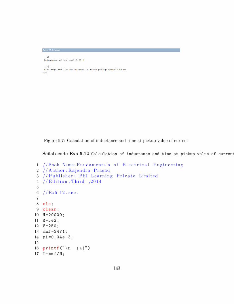
Figure 5.7: Calculation of inductance and time at pickup value of current
Scilab code Exa 5.12 Calculation of inductance and time at pickup value of current
1 // Book Name : Fundamentals o f E l e c t r i c a l E n g i n e e r i n g2 // Author : Rajendra Prasad3 // P u b l i s h e r : PHI Lea rn ing P r i v a t e L imi ted4 // E d i t i o n : Third ,20145
6 // Ex5 12 . s c e .7
8 clc;
9 clear;
10 N=20000;
11 R=5e2;
12 V=250;
13 mmf =3471;
14 pi=0.04e-3;
15
16 printf(”\n ( a ) ”)17 I=mmf/N;
143

Figure 5.8: Calculation of cross sectional area of the core and magnetizingcurrent
18 L=(N*pi)/I;
19 printf(”\n Induc tance o f the c o i l=%1 . 2 f H \n”,L)20
21 printf(”\n ( b ) ”)22 t=log (1/(1 -((I*R)/V)))*(L/R);
23 printf(”\n Time r e q u i r e d f o r the c u r r e n t to r ea chp ickup v a l u e=%1 . 2 f ms”,t*1E3)
24 //The book answer f o r t (=3.93 ms) i s o b t a i n e d on lyi f R=500 ohm . Otherwi s e (R=5000) we cannot g e t theanswer
25 // So t h e r e i s a mi s take i n R v a l u e g i v e n
Scilab code Exa 5.13 Calculation of cross sectional area of the core and magnetizing current
144

1 // Book Name : Fundamentals o f E l e c t r i c a l E n g i n e e r i n g2 // Author : Rajendra Prasad3 // P u b l i s h e r : PHI Lea rn ing P r i v a t e L imi ted4 // E d i t i o n : Third ,20145
6 // Ex5 13 . s c e .7
8 clc;
9 clear;
10 Bm=1.1;
11 V=2.2e3;
12 f=50;
13 N=200;
14
15 printf(”\n\ t ( a ) ”)16 stack_factor =0.9;
17 pi_m=V/(4.44*f*N);
18 A=pi_m/(Bm*stack_factor);
19 printf(”\n Cross s e c t i o n a l a r ea o f the c o r e=%3 . 1 fcmˆ2 \n”,A*1e4)
20 // There i s a s m a l l ( p r i n t i n g ) mi s take i n the f i n a lanswer o f A i n the book
21
22 printf(”\n\ t ( b ) ”)23 l=250e-2;
24 H=490; // from the graph 5 . 2 1 H v a l u e i staken which i s c o r r e s p o n d i n g to B=1.1 wb/mˆ2
25 mmf=H*l;
26 Im=mmf/N;
27 printf(”\n Magnet i z ing c u r r e n t=%1 . 3 f A”,Im)
Scilab code Exa 5.14 Determination of steady state value of current and resistance and inductance of the coil and stored energy
145

Figure 5.9: Determination of steady state value of current and resistance andinductance of the coil and stored energy
1 // Book Name : Fundamentals o f E l e c t r i c a l E n g i n e e r i n g2 // Author : Rajendra Prasad3 // P u b l i s h e r : PHI Lea rn ing P r i v a t e L imi ted4 // E d i t i o n : Third ,20145
6 // Ex5 14 . s c e .7
8 clc;
9 clear;
10 V=200;
11 i=0.2;
12 T=3e-3;
13 t=3e-3;
14
15 R=(V/i)*(1-exp(-t/T));
16 I=V/R;
17 printf(”\n The f i n a l s t e ady s t a t e v a l u e o f c u r r e n t=%1 . 3 f A \n”,I)
146

Figure 5.10: Calculation of load current and impedence referred to primaryand secondary side
18
19 L=R*T;
20 printf(”\n Induc tance=%1 . 3 f H \n”,L)21 printf(”\n R e s i s t a n c e=%3 . 0 f ohm \n”,R)22
23 E=(L*I^2) /2;
24 printf(”\n Energy s t o r e d when c u r r e n t r eached i t sf i n a l v a l u e=%1 . 3 f J”,E)
Scilab code Exa 5.15 Calculation of load current and impedence referred to primary and secondary side
1 // Book Name : Fundamentals o f E l e c t r i c a l E n g i n e e r i n g2 // Author : Rajendra Prasad
147

3 // P u b l i s h e r : PHI Lea rn ing P r i v a t e L imi ted4 // E d i t i o n : Third ,20145
6 // Ex5 15 . s c e .7
8 clc;
9 clear;
10 P=50e3;
11 V1=2.2e3;
12 V2=220;
13
14 printf(”\n ( a ) ”)15 I1=P/V1;
16 I2=P/V2;
17 printf(”\n Primary c u r r e n t=%2 . 2 f A \n”,I1)18 printf(”\n Secondary c u r r e n t=%3 . 1 f A \n”,I2)19
20 printf(”\n ( b ) ”)21 Zl2=V2/I2;
22 printf(”\n The l oad impedence f o r the s e conda ry s i d e=%1 . 3 f ohm \n”,Zl2)
23
24 printf(”\n ( c ) ”)25 Zl1=V1/I1;
26 printf(”\n The l oad impedence f o r the pr imary s i d e=%2 . 1 f ohm \n”,Zl1)
Scilab code Exa 5.16 Calculation of instantaneous values of induced emf
1 // Book Name : Fundamentals o f E l e c t r i c a l E n g i n e e r i n g2 // Author : Rajendra Prasad3 // P u b l i s h e r : PHI Lea rn ing P r i v a t e L imi ted4 // E d i t i o n : Third ,2014
148

Figure 5.11: Calculation of instantaneous values of induced emf
5
6 // Ex5 16 . s c e .7
8 clc;
9 clear;
10 N=100;
11 a=10e-2;
12 n=20;
13 B=0.5;
14
15 omega =2* %pi*n;
16 A=a^2;
17 v=A*N*omega*B;
18
19 printf(”\n ( a ) ”)20 // t h e t a =40∗180∗ t=n∗180 where n = 0 , 1 , 2 , 3 . . . . .21 // i f we take n=222 V=v*sind (180*2);
23 printf(”\n The i n s t a n t a n e o u s v a l u e o f induced emfwhen p l ane o f the c o i l i s r i g h t a n g l e to thef i e l d =%d v o l t \n”,V)
24
25 printf(”\n ( b ) ”)26 // t h e t a=n∗180/2 where n = 1 , 3 , 5 , 7 . . . . . . . . .
149

Figure 5.12: Determination of torque exerted on the coil
27 // i f we take n=328 V=v*sind (180*3/2);
29 printf(”\n The i n s t a n t a n e o u s v a l u e o f induced emfwhen the p l ane o f the c o i l i s i n the p l ane o f the
f i e l d =%2 . 1 f v o l t ”,V)
Scilab code Exa 5.17 Determination of torque exerted on the coil
1 // Book Name : Fundamentals o f E l e c t r i c a l E n g i n e e r i n g2 // Author : Rajendra Prasad3 // P u b l i s h e r : PHI Lea rn ing P r i v a t e L imi ted4 // E d i t i o n : Third ,20145
6 // Ex5 17 . s c e .
150

7
8 clc;
9 clear;
10 l=7.5e-2;
11 b=5e-2;
12 N=100;
13 B=1.1;
14 i=5;
15 T=N*B*l*b*i;
16 printf(”\n Torque e x e r t e d on the c o i l=%1 . 4 f Nm”,T)
151

Chapter 7
Transformer
Scilab code Exa 7.1 Calculation of current and number of turns and maximum flux value
1 // Book Name : Fundamentals o f E l e c t r i c a l E n g i n e e r i n g2 // Author : Rajendra Prasad3 // P u b l i s h e r : PHI Lea rn ing P r i v a t e L imi ted4 // E d i t i o n : Third ,20145
6 // Ex7 1 . s c e .7
8 clc;
9 clear;
10 p=175e3; // power r a t i n g o ft r a n s f o r m e r i n KVA
11 Ep =6600; // pr imary v o l t a g e i nv o l t s
12 Es=440; // s e condary v o l t a g e i nv o l t s
13 f=50;
14 Ns=100; //Number o f s e conda ryt u r n s
15
152

Figure 7.1: Calculation of current and number of turns and maximum fluxvalue
153
16 // ( a )17 printf(”\n ( a ) ”)18 Ip=p/Ep;
19 Is=p/Es;
20 printf(”\n F u l l l o ad pr imary c u r r e n t=%2 . 2 f A ”,Ip)21 printf(”\n F u l l l o ad s e conda ry c u r r e n t=%3 . 2 f A \n”,
Is)
22
23 // ( b )24 printf(”\n ( b ) ”)25 Np=Ns*Ep/Es;
26 printf(”\n Number o f pr imary t u r n s=%d \n”,Np)27
28 // ( c )29 printf(”\n ( c ) ”)30 max_flux=Es /(4.44*f*Ns);
31 printf(”\n The maximum v a l u e o f f l u x=%1 . 5 f Wb \n”,max_flux)
Scilab code Exa 7.2 Calculation of primary current and power factor
1 // Book Name : Fundamentals o f E l e c t r i c a l E n g i n e e r i n g2 // Author : Rajendra Prasad3 // P u b l i s h e r : PHI Lea rn ing P r i v a t e L imi ted4 // E d i t i o n : Third ,20145
6 // Ex7 2 . s c e .7
8 clc;
9 clear;
10 Np =1000; // number o fPrimary t u r n s
11 Ns=200; // number o f
154
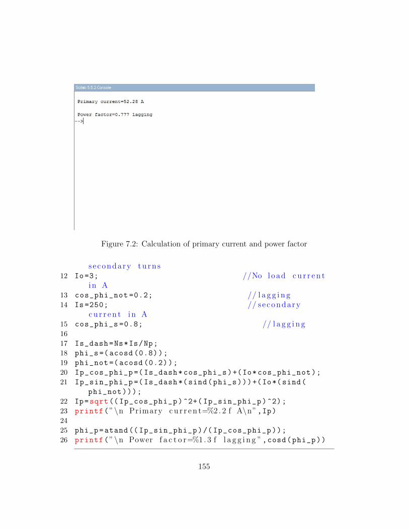
Figure 7.2: Calculation of primary current and power factor
s e condary t u r n s12 Io=3; //No load c u r r e n t
i n A13 cos_phi_not =0.2; // l a g g i n g14 Is=250; // s e condary
c u r r e n t i n A15 cos_phi_s =0.8; // l a g g i n g16
17 Is_dash=Ns*Is/Np;
18 phi_s=(acosd (0.8));
19 phi_not =( acosd (0.2));
20 Ip_cos_phi_p =( Is_dash*cos_phi_s)+(Io*cos_phi_not);
21 Ip_sin_phi_p =( Is_dash *(sind(phi_s)))+(Io*(sind(
phi_not)));
22 Ip=sqrt(( Ip_cos_phi_p)^2+( Ip_sin_phi_p)^2);
23 printf(”\n Primary c u r r e n t=%2 . 2 f A\n”,Ip)24
25 phi_p=atand (( Ip_sin_phi_p)/( Ip_cos_phi_p));
26 printf(”\n Power f a c t o r=%1 . 3 f l a g g i n g ”,cosd(phi_p))
155

Figure 7.3: Determination of primary current and power factor and secondaryterminal voltage
Scilab code Exa 7.3 Determination of primary current and power factor and secondary terminal voltage
1 // Book Name : Fundamentals o f E l e c t r i c a l E n g i n e e r i n g2 // Author : Rajendra Prasad3 // P u b l i s h e r : PHI Lea rn ing P r i v a t e L imi ted4 // E d i t i o n : Third ,20145
6 // Ex7 3 . s c e .7
8 clc;
9 clear;
156
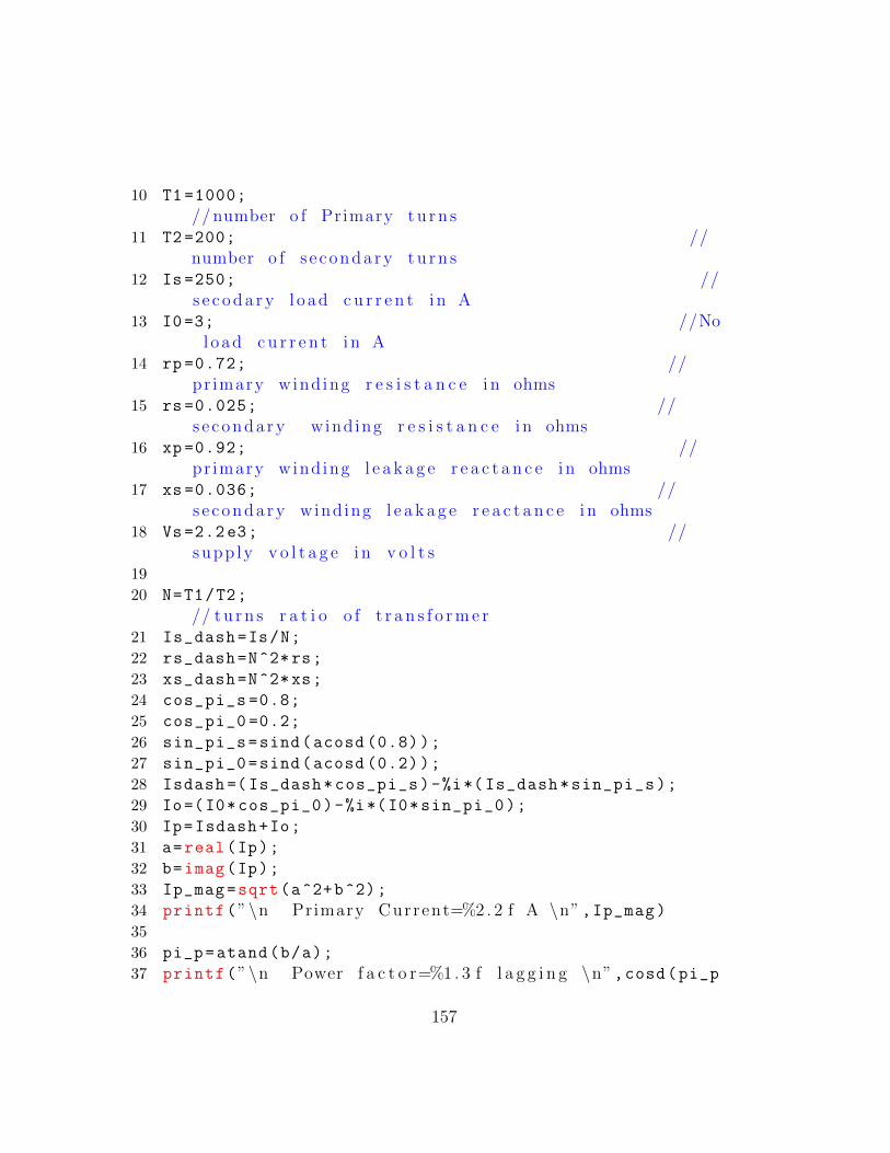
10 T1 =1000;
// number o f Primary t u r n s11 T2=200; //
number o f s e conda ry t u r n s12 Is=250; //
s e c o d a r y l oad c u r r e n t i n A13 I0=3; //No
load c u r r e n t i n A14 rp =0.72; //
pr imary winding r e s i s t a n c e i n ohms15 rs =0.025; //
s e condary wind ing r e s i s t a n c e i n ohms16 xp =0.92; //
pr imary winding l e a k a g e r e a c t a n c e i n ohms17 xs =0.036; //
s e condary wind ing l e a k a g e r e a c t a n c e i n ohms18 Vs=2.2e3; //
supp ly v o l t a g e i n v o l t s19
20 N=T1/T2;
// t u r n s r a t i o o f t r a n s f o r m e r21 Is_dash=Is/N;
22 rs_dash=N^2*rs;
23 xs_dash=N^2*xs;
24 cos_pi_s =0.8;
25 cos_pi_0 =0.2;
26 sin_pi_s=sind(acosd (0.8));
27 sin_pi_0=sind(acosd (0.2));
28 Isdash =( Is_dash*cos_pi_s)-%i*( Is_dash*sin_pi_s);
29 Io=(I0*cos_pi_0)-%i*(I0*sin_pi_0);
30 Ip=Isdash+Io;
31 a=real(Ip);
32 b=imag(Ip);
33 Ip_mag=sqrt(a^2+b^2);
34 printf(”\n Primary Current=%2 . 2 f A \n”,Ip_mag)35
36 pi_p=atand(b/a);
37 printf(”\n Power f a c t o r=%1 . 3 f l a g g i n g \n”,cosd(pi_p
157

Figure 7.4: Calculation of impedence and voltage regulation
))
38
39 VL_dash=Vs -(Ip*(rp+%i*xp))-(Isdash *( rs_dash+%i*
xs_dash)); // s e condary t e r m i n a lv o l t a g e r e f e r r e d to pr imary
40 VL_dash_mag=real(VL_dash);
41 VL=VL_dash_mag/N;
42 printf(”\n Secondary t e r m i n a l v o l t a g e=%3 . 1 f V \n”,VL)
Scilab code Exa 7.4 Calculation of impedence and voltage regulation
1 // Book Name : Fundamentals o f E l e c t r i c a l E n g i n e e r i n g2 // Author : Rajendra Prasad3 // P u b l i s h e r : PHI Lea rn ing P r i v a t e L imi ted4 // E d i t i o n : Third ,2014
158

5
6 // Ex7 4 . s c e .7
8 clc;
9 clear;
10 P=75e3; // power r a t i n g o ft r a n s f o r m e r i n KVA
11 Np=500; // number o fPrimary t u r n s
12 Ns=100; // number o fs e conda ry t u r n s
13 rp=0.4; // pr imarywind ing r e s i s t a n c e i n ohms
14 rs =0.02; // s e condarywind ing r e s i s t a n c e i n ohms
15 xp=1.5; // pr imary wind ingl e a k a g e r e a c t a n c e i n ohms
16 xs =0.045; // s e condarywind ing l e a k a g e r e a c t a n c e i n ohms
17 Vs =2200; // supp ly v o l t a g ei n v o l t s
18
19 // c a s e 120 printf(”\n ( a ) ”)21 Re=rp+(Np/Ns)^2*rs; //
E q u i v a l e n t r e s i s t a n c e i n ohms22 Xe=xp+(Np/Ns)^2*xs; //
E q u i v a l e n t l e a k a g e r e a c t a n c e i n ohms23 Ze=sqrt(Re^2+Xe^2);
24 printf(”\n E q u i v a l e n t impedance r e f e r r e d topr inmary s i d e=%1 . 3 f ohms\n”,Ze)
25
26 // c a s e 227 printf(”\n ( b ) . 1 ”)28 I1=P/Vs; //
f u l l l o ad pr imary c u r r e n t i n A29 cos_pi2 =0.8;
30 sin_pi2=sind(acosd (0.8));
159

31 percentage_voltage_reg =((I1*((Re*cos_pi2)+(Xe*
sin_pi2)))/Vs)*100;
32 printf(”\n Vo l tage r e g u l a t i o n f o r 0 . 8 power f a c t o rl a g g i n g=%1 . 2 f p e r c e n t a g e \n”,percentage_voltage_reg)
33 NL_secondary_voltage =(Ns/Np)*Vs;
//NL means ”no l oad ”34 del_V=( NL_secondary_voltage*percentage_voltage_reg)
/100;
35 FL_secondary_voltage =( NL_secondary_voltage) -(del_V);
36 printf(”\n Secodary t e r m i n a l v o l t a g e at FL 0 . 8power f a c t o r l a g g i n g=%3 . 3 f V \n”,FL_secondary_voltage)
37
38 // c a s e 339 printf(”\n ( b ) . 2 ”)40 percentage_voltage_reg =((I1*((Re*cos_pi2) -(Xe*
sin_pi2)))/Vs)*100;
41 printf(”\n Vo l tage r e g u l a t i o n f o r 0 . 8 power f a c t o rl e a d i n g=%1 . 3 f p e r c e n t a g e \n”,percentage_voltage_reg)
42 del_V=( NL_secondary_voltage*percentage_voltage_reg)
/100;
43 FL_secondary_voltage =( NL_secondary_voltage) -(del_V);
44 printf(”\n Secodary t e r m i n a l v o l t a g e at FL 0 . 8power f a c t o r l e a d i n g=%4 . 4 f V \n”,FL_secondary_voltage)
45 //The anwser vary dueto r o u n d o f f e r r o r
Scilab code Exa 7.5 Calculation of efficiency
1 // Book Name : Fundamentals o f E l e c t r i c a l E n g i n e e r i n g
160
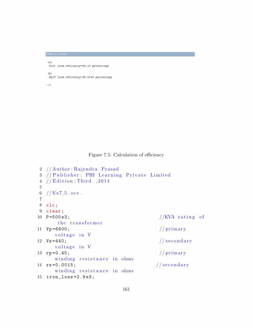
Figure 7.5: Calculation of efficiency
2 // Author : Rajendra Prasad3 // P u b l i s h e r : PHI Lea rn ing P r i v a t e L imi ted4 // E d i t i o n : Third ,20145
6 // Ex7 5 . s c e .7
8 clc;
9 clear;
10 P=500e3; //KVA r a t i n g o fthe t r a n s f o r m e r
11 Vp =6600; // pr imaryv o l t a g e i n V
12 Vs=440; // s e condaryv o l t a g e i n V
13 rp =0.45; // pr imarywind ing r e s i s t a n c e i n ohms
14 rs =0.0015; // s e condarywind ing r e s i s t a n c e i n ohms
15 iron_loss =2.9e3;
161

16 pf=0.8; // power f a c t o rl a g g i n g
17
18 // c a s e 119 printf(”\n ( a ) ”)20 Ip=P/Vp; // pr imary
c u r r e n t i n A21 Is=P/Vs; //
s e condary c u r r e n t i n A22 Ip_square_rp=Ip^(2)*rp;
// pr imarycopper l o s s
23 Is_square_rs=Is^(2)*rs;
// s e condarycopper l o s s
24 FL_copper_loss=Ip_square_rp+Is_square_rs;
//FL means ” f u l l l o ad ”25 FL_total_loss=iron_loss+FL_copper_loss;
26 FL_output_power=P*pf;
27 FL_input_power=FL_output_power+FL_total_loss;
28 FL_efficiency =( FL_output_power/FL_input_power)*100;
29 printf(”\n F u l l l o ad e f f i c i e n c y=%2 . 2 f p e r c e n t a g e \n”,FL_efficiency)
30
31 // c a s e 232 printf(”\n ( b ) ”)33 HL_copper_loss=FL_copper_loss *(0.5^2);
//HL means ”h a l f l o ad ”
34 HL_total_loss=iron_loss+HL_copper_loss;
35 HL_output_power=FL_output_power /2;
36 HL_input_power=HL_output_power+HL_total_loss;
37 HL_efficiency =( HL_output_power/HL_input_power)*100;
38 printf(”\n Ha l f l o ad e f f i c i e n c y=%2 . 4 f p e r c e n t a g e \n”,HL_efficiency)
162

Figure 7.6: Calculation of maximum efficiency
Scilab code Exa 7.6 Calculation of maximum efficiency
1 // Book Name : Fundamentals o f E l e c t r i c a l E n g i n e e r i n g2 // Author : Rajendra Prasad3 // P u b l i s h e r : PHI Lea rn ing P r i v a t e L imi ted4 // E d i t i o n : Third ,20145
6 // Ex7 6 . s c e .7
8 clc;
163

9 clear;
10 // the g i v e n data a r e taken from p r e v i o u s example (Ex7 5 )
11
12 Vp =6600; //pr imary v o l t a g e i n V
13 Vs=440; //s e condary v o l t a g e i n V
14 rp =0.45; // pr imarywind ing r e s i s t a n c e i n ohms
15 rs =0.0015; // s e condarywind ing r e s i s t a n c e i n ohms
16 Wi=2.9e3; // i r o nl o s s i n watt
17 pf=0.8; // powerf a c t o r l a g g i n g
18
19 Re=rp+(Vp/Vs)^2*rs; // e q u i v a l e n tr e s i s t a n c e r e f e r r e d to pr imary
20 Ip=sqrt(Wi/Re);
21 P_max=Vp*Ip*pf;
22 total_loss =2*Wi;
23 Max_efficiency =(P_max /( P_max+total_loss))*100;
24 printf(”\n Maximum E f f i c i e n c y=%2 . 2 f p e r c e n t a g e \n”,Max_efficiency)
Scilab code Exa 7.7 Calculation of efficiency and voltage regulation and secondary terminal voltage
1 // Book Name : Fundamentals o f E l e c t r i c a l E n g i n e e r i n g2 // Author : Rajendra Prasad3 // P u b l i s h e r : PHI Lea rn ing P r i v a t e L imi ted4 // E d i t i o n : Third ,20145
164

Figure 7.7: Calculation of efficiency and voltage regulation and secondaryterminal voltage
6 // Ex7 7 . s c e7 clc;
8 clear;
9 KVA =50e3;
10
11 printf(”\n ( a ) ”)12 PF=0.7;
13 iron_loss =430; // pr imary power o ft r a n s f o r m e r on open c i r c u i t t e s t i n watt i sc a l l e d i r o n l o s s
14 copper_loss_FL =525; // pr imary power o ft r a n s f o r m e r on s h o r t c i r c u i t t e s t i n watt i sc a l l e d copper l o s s
15 total_loss_FL=iron_loss+copper_loss_FL;
16 eta_FL =(KVA*PF)/((KVA*PF)+total_loss_FL)*100;
// f u l l l o ad e f f i c i e n c y17 printf(”\n F u l l l o ad e f f i c i e n c y f o r 0 . 7 power
f a c t o r=%2 . 2 f p e r c e n t a g e \n”,eta_FL)18 copper_loss_HL =(0.5^2)*copper_loss_FL;
19 total_loss_HL=iron_loss+copper_loss_HL;
20 eta_HL =(KVA*PF*0.5) /((KVA *0.5* PF)+total_loss_HL)
165
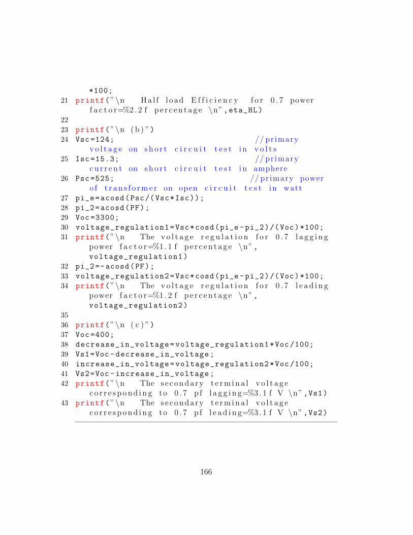
*100;
21 printf(”\n Ha l f l o ad E f f i c i e n c y f o r 0 . 7 powerf a c t o r=%2 . 2 f p e r c e n t a g e \n”,eta_HL)
22
23 printf(”\n ( b ) ”)24 Vsc =124; // pr imary
v o l t a g e on s h o r t c i r c u i t t e s t i n v o l t s25 Isc =15.3; // pr imary
c u r r e n t on s h o r t c i r c u i t t e s t i n amphere26 Psc =525; // pr imary power
o f t r a n s f o r m e r on open c i r c u i t t e s t i n watt27 pi_e=acosd(Psc/(Vsc*Isc));
28 pi_2=acosd(PF);
29 Voc =3300;
30 voltage_regulation1=Vsc*cosd(pi_e -pi_2)/(Voc)*100;
31 printf(”\n The v o l t a g e r e g u l a t i o n f o r 0 . 7 l a g g i n gpower f a c t o r=%1 . 1 f p e r c e n t a g e \n”,voltage_regulation1)
32 pi_2=-acosd(PF);
33 voltage_regulation2=Vsc*cosd(pi_e -pi_2)/(Voc)*100;
34 printf(”\n The v o l t a g e r e g u l a t i o n f o r 0 . 7 l e a d i n gpower f a c t o r=%1 . 2 f p e r c e n t a g e \n”,voltage_regulation2)
35
36 printf(”\n ( c ) ”)37 Voc =400;
38 decrease_in_voltage=voltage_regulation1*Voc /100;
39 Vs1=Voc -decrease_in_voltage;
40 increase_in_voltage=voltage_regulation2*Voc /100;
41 Vs2=Voc -increase_in_voltage;
42 printf(”\n The s e conda ry t e r m i n a l v o l t a g ec o r r e s p o n d i n g to 0 . 7 p f l a g g i n g=%3 . 1 f V \n”,Vs1)
43 printf(”\n The s e conda ry t e r m i n a l v o l t a g ec o r r e s p o n d i n g to 0 . 7 p f l e a d i n g=%3 . 1 f V \n”,Vs2)
166

Figure 7.8: Calculation of primary line current and voltage and line to linetransformation ratio
167

Scilab code Exa 7.8 Calculation of primary line current and voltage and line to line transformation ratio
1 // Book Name : Fundamentals o f E l e c t r i c a l E n g i n e e r i n g2 // Author : Rajendra Prasad3 // P u b l i s h e r : PHI Lea rn ing P r i v a t e L imi ted4 // E d i t i o n : Third ,20145
6 // Ex7 8 . s c e .7
8 clc;
9 clear;
10 Np =1000; // number o fPrimary t u r n s
11 Ns=100; // number o fs e conda ry t u r n s
12 KVA =120e3; //KVAr a t i n g o f the t r a n s f o r m e r
13 V_SL =440; // supp lyv o l t a g e i n V
14
15 K=Np/Ns; // t r a n s f o r m e rt u r n s r a t i o
16 I_SL=KVA/(sqrt (3)*V_SL);
17
18 printf(”\n ( a ) ”)19 V_PL=(V_SL*K)/sqrt (3);
20 I_PL=(sqrt (3)*I_SL)/K;
21 transformation_ratio=V_PL/V_SL;
22 printf(”\n De l ta s t a r c o n n e c t i o n : \ n”)23 printf(”\n Primary l i n e c u r r e n t=%2 . 1 f A ”,I_PL)24 printf(”\n Primary l i n e v o l t a g e=%d V ”,V_PL)25 printf(”\n Trans f o rmat i on r a t i o =%2 . 1 f \n”,
transformation_ratio)
26
168

Figure 7.9: Determination of position of tapping point and current in eachpart of winding and copper saved
27 printf(”\n ( b ) ”)28 V_PL=V_SL*K*sqrt (3);
29 I_PL=I_SL/(sqrt (3)*K);
30 transformation_ratio=V_PL/V_SL;
31 printf(”\n s t a r d e l t a c o n n e c t i o n : \ n”)32 printf(”\n Primary l i n e c u r r e n t=%1 . 1 f A ”,I_PL)33 printf(”\n Primary l i n e v o l t a g e=%d V ”,V_PL)34 printf(”\n Trans f o rmat i on r a t i o =%2 . 2 f ”,
transformation_ratio)
Scilab code Exa 7.9 Determination of position of tapping point and current in each part of winding and copper saved
1 // Book Name : Fundamentals o f E l e c t r i c a l E n g i n e e r i n g2 // Author : Rajendra Prasad3 // P u b l i s h e r : PHI Lea rn ing P r i v a t e L imi ted4 // E d i t i o n : Third ,20145
169

6 // Ex7 9 . s c e .7
8 clc;
9 clear;
10 Vp=220; //pr imary v o l t a g e i n V
11 Vs=250; //s e condary v o l t a g e i n V
12 Ns =2000; //number o f s e conda ry t u r n s
13
14 printf(”\n ( a ) ”)15 Np=(Vp/Vs)*Ns; //
number o f Primary t u r n s16 tapping_point=Ns-Np; //
number o f t u r n s from C to A i n f i g u r e17 printf(”\n The p o s i t i o n o f t app ing p o i n t=%d t u r n s \
n”,tapping_point)18
19 printf(”\n ( b ) ”)20 Po=10e3; // output
power i n KVA21 Is=Po/Vs; //
s e c o d a r y c u r r e n t i n A22 Ip=(Vs/Vp)*Is; //
pr imary c u r r e n t i n A23 approximate_current=Ip -Is;
24 printf(”\n The approx imate v a l u e o f c u r r e n t i n eachpa r t o f the wind ing : \ n”)
25 printf(”\ t I s=%d A\n”,Is)26 printf(”\ t Ip=%2 . 2 f A\n”,Ip)27 printf(”\ t Ip−I s=%1 . 2 f A\n”,approximate_current)28
29 printf(”\n ( c ) ”)30 copper_saved=Vp/Vs;
31 printf(”\n copper saved=%1 . 2 f p . u”,copper_saved)
170

Figure 7.10: Determination of ratio error
Scilab code Exa 7.10 Determination of ratio error
1 // Book Name : Fundamentals o f E l e c t r i c a l E n g i n e e r i n g2 // Author : Rajendra Prasad3 // P u b l i s h e r : PHI Lea rn ing P r i v a t e L imi ted4 // E d i t i o n : Third ,20145
6 // Ex7 10 . s c e .7
8 clc;
9 clear;
10 Ip =1000; // pr imary c u r r e n ti n A
11 Is=5; // s e c o d a r y c u r r e n ti n A
12 Tp=1; // number o fPrimary t u r n s
13
14 printf(”\n ( a ) ”)
171
15 nominal_ratio=Ip/Is;
16 Ie=7; // l o s s componento f c u r r e n t i n A
17 actual_ratio=nominal_ratio +(Ie/Is);
18 epsilon_r =(( nominal_ratio -actual_ratio)/actual_ratio
)*100;
19 printf(”\n Rat io e r r o r when t u r n s r a t i o e q u a l tonominal r a t i o=%1 . 3 f p e r c e n t a g e \n”,epsilon_r)
20
21 printf(”\n ( b ) ”)22 reducing_value =0.5/100;
23 Ts=nominal_ratio -( reducing_value*nominal_ratio);
24 n=Ts/Tp; //t r a n s f o r m e r t u r n s r a t i o
25 actual_ratio=n+(Ie/Is);
26 epsilon_r =(( nominal_ratio -actual_ratio)/actual_ratio
)*100;
27 printf(”\n Rat io e r r o r when se conda ry t u r n s a r ereduced by 0 . 5 p e r c e n t a g e=%1 . 1 f p e r c e n t a g e ”,epsilon_r)
172

Chapter 8
Direct Current Machines
Scilab code Exa 8.1 Calculation of design parameters for a dc machine
1 // Book Name : Fundamentals o f E l e c t r i c a l E n g i n e e r i n g2 // Author : Rajendra Prasad3 // P u b l i s h e r : PHI Lea rn ing P r i v a t e L imi ted4 // E d i t i o n : Third ,20145
6 // Ex8 1 . s c e7
8 clc;
9 clear;
10 p=4;
11 s=24;
12 com_seg =24;
13 // wind ing d e t a i l c a l c u l a t i o n14 pole_pitch=s/p;
15 c=com_seg;
16 printf(”\n Number o f c o i l s=%d \n”,c)17 Cs=2*c;
18 printf(”\n Number o f c o i l s i d e s=%d \n”,Cs)19 Yb1=Cs/p+1;
173

Figure 8.1: Calculation of design parameters for a dc machine
20 Yb2=Cs/p-1;
21 Yb=Yb1; // c h o o s i n g f u l l p i t c h c o i l22 printf(”\n Back p i t c h=%d \n”,Yb)23 Yf1=Yb -2; // For p r o g r e s s i v e wind ing24 Yf2=Yb+2; // For r e t r o g r e s s i v e wind ing25 Yf=Yf1;
26 printf(”\n F u l l p i t c h=%d \n”,Yf)27 // f o r p r o g r e s s i v e wind ing28 Y=2;
29 Yc=1;
30 printf(”\n Winding p i t c h=%d \n”,Y)31 printf(”\n Commutator p i t c h=%d \n”,Yc)
Scilab code Exa 8.2 Calculation of design parameters for a dc machine
174

Figure 8.2: Calculation of design parameters for a dc machine
1 // Book Name : Fundamentals o f E l e c t r i c a l E n g i n e e r i n g2 // Author : Rajendra Prasad3 // P u b l i s h e r : PHI Lea rn ing P r i v a t e L imi ted4 // E d i t i o n : Third ,20145
6 // Ex8 2 . s c e7
8 clc;
9 clear;
10 p=4;
11 s=30;
12 c=90;
13 Cs=2*c;
14 printf(”\n Number o f c o i l s i d e s=%d \n”,Cs)15 Cs_per_slot=Cs/s;
16 printf(”\n Number o f c o i l s i d e s per s l o t=%d \n”,Cs_per_slot)
17 Yb1=Cs/p+2; // Winding i s not s p l i t18 Yb2=Cs/p-2; // Winding i s s p l i t
175

Figure 8.3: Calculation of design parameters for a dc machine
19 Yb=Yb2;
20 printf(”\n Back p i t c h=%d \n”,Yb)21 Cs1 =1+Yb;
22 Cs3 =3+Yb;
23 Cs5 =5+Yb;
24 //Top c o i l s i d e s 1 , 3 , 5 a r e i n i n s l o t , w h i l e a l l thec o r r e s p o n d i n g bottom c o i l s i d e s 44 , 46 , 48 a r e i ns l o t 8 .
Scilab code Exa 8.3 Calculation of design parameters for a dc machine
1 // Book Name : Fundamentals o f E l e c t r i c a l E n g i n e e r i n g2 // Author : Rajendra Prasad3 // P u b l i s h e r : PHI Lea rn ing P r i v a t e L imi ted4 // E d i t i o n : Third ,20145
6 // Ex8 3 . s c e7
176
8 clc;
9 clear;
10 s=25;
11 c=25;
12 com_seg =25;
13 p=4;
14 Sp=s/p; // s l o t per p o l e15 printf(”\n S l o t s per p o l e=%d \n”,Sp)16 Cs=2*c;
17 printf(”\n Number o f c o i l s i d e s=%d \n”,Cs)18 Cs_per_slot=Cs/s;
19 printf(”\n Number o f c o i l s i d e s per s l o t=%d \n”,Cs_per_slot)
20 Y1=((2*c)+2)/(p/2);
21 Y2=((2*c) -2)/(p/2);
22 Y=Y1; // For p r o g r e s s i v e wind ing23 printf(”\n Winding p i t c h=%d \n”,Y)24 Yb=Y/2;
25 printf(”\n Back p i t c h=%d \n”,Yb)26 Yf=Yb;
27 printf(”\n F u l l p i t c h=%d \n”,Yf)28 Yc=(c+1)/(p/2);
29 printf(”\n Commutator p i t c h=%d \n”,Yc)
Scilab code Exa 8.4 Calculation of design parameters for a dc machine
1 // Book Name : Fundamentals o f E l e c t r i c a l E n g i n e e r i n g2 // Author : Rajendra Prasad3 // P u b l i s h e r : PHI Lea rn ing P r i v a t e L imi ted4 // E d i t i o n : Third ,20145
6 // Ex8 4 . s c e7
177
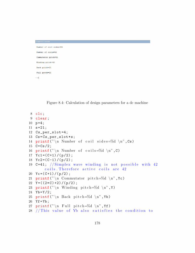
Figure 8.4: Calculation of design parameters for a dc machine
8 clc;
9 clear;
10 p=4;
11 s=21;
12 Cs_per_slot =4;
13 Cs=Cs_per_slot*s;
14 printf(”\n Number o f c o i l s i d e s=%d \n”,Cs)15 C=Cs/2;
16 printf(”\n Number o f c o i l s=%d \n”,C)17 Yc1=(C+1)/(p/2);
18 Yc2=(C-1)/(p/2);
19 C=41; // Simplex wave wind ing i s not p o s s i b l e with 42c o i l s . T h e r e f o r e a c t i v e c o i l s a r e 42
20 Yc=(C+1)/(p/2);
21 printf(”\n Commutator p i t c h=%d \n”,Yc)22 Y=((2*C)+2)/(p/2);
23 printf(”\n Winding p i t c h=%d \n”,Y)24 Yb=Y/2;
25 printf(”\n Back p i t c h=%d \n”,Yb)26 Yf=Yb;
27 printf(”\n F u l l p i t c h=%d \n”,Yf)28 // This v a l u e o f Yb a l s o s a t i s f i e s the c o n d i t i o n to
178

Figure 8.5: Calculation of generated emf
avo id s p l i t wind ing
Scilab code Exa 8.5 Calculation of generated emf
1 // Book Name : Fundamentals o f E l e c t r i c a l E n g i n e e r i n g2 // Author : Rajendra Prasad3 // P u b l i s h e r : PHI Lea rn ing P r i v a t e L imi ted4 // E d i t i o n : Third ,20145
6 // Ex8 5 . s c e .7
8 clc;
9 clear;
10 s=50;
11 c=8;
12 N=900;
179
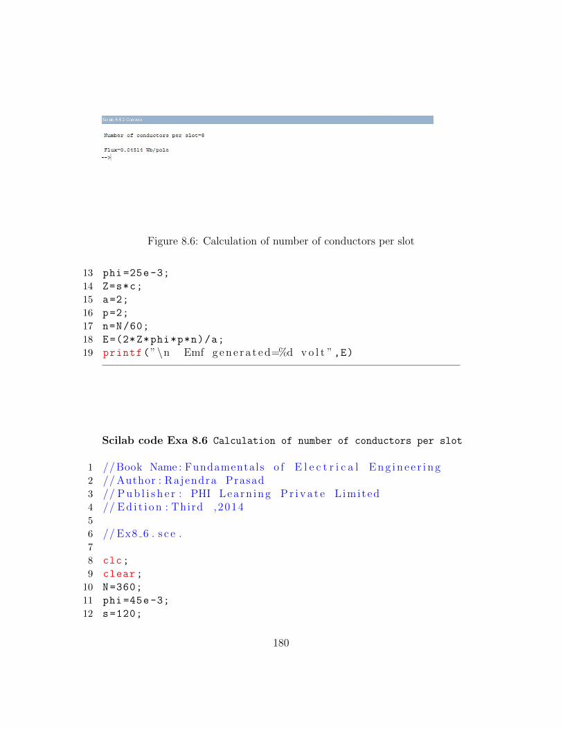
Figure 8.6: Calculation of number of conductors per slot
13 phi =25e-3;
14 Z=s*c;
15 a=2;
16 p=2;
17 n=N/60;
18 E=(2*Z*phi*p*n)/a;
19 printf(”\n Emf g e n e r a t e d=%d v o l t ”,E)
Scilab code Exa 8.6 Calculation of number of conductors per slot
1 // Book Name : Fundamentals o f E l e c t r i c a l E n g i n e e r i n g2 // Author : Rajendra Prasad3 // P u b l i s h e r : PHI Lea rn ing P r i v a t e L imi ted4 // E d i t i o n : Third ,20145
6 // Ex8 6 . s c e .7
8 clc;
9 clear;
10 N=360;
11 phi =45e-3;
12 s=120;
180

Figure 8.7: Calculation of number of demagnetizing and cross ampere turnsper pole
13 E=260;
14 p=4;
15 n=N/60;
16 a=8;
17 Z=(E*a)/(2* phi*p*n);
18 coductors_per_slot=Z/s;
19 total_no_of_conductors=coductors_per_slot*s;
20 printf(”\n Number o f c o n d u c t o r s per s l o t=%d \n”,coductors_per_slot)
21
22 phi=(E*a)/(2*960*n*p)
23 printf(”\n Flux=%1 . 5 f Wb/ p o l e ”,phi)
Scilab code Exa 8.7 Calculation of number of demagnetizing and cross ampere turns per pole
1 // Book Name : Fundamentals o f E l e c t r i c a l E n g i n e e r i n g2 // Author : Rajendra Prasad3 // P u b l i s h e r : PHI Lea rn ing P r i v a t e L imi ted
181

4 // E d i t i o n : Third ,20145
6 // Ex8 7 . s c e .7
8 clc;
9 clear;
10 P=300e3;
11 V=500;
12 a=8;
13 p=4;
14 Z=786;
15 theta =5;
16
17 I=P/V;
18 armature_AT =(1/2) *(I/a)*(Z/(2*p)); //Tota l AT per p o l e
19 demagnetizing_AT=armature_AT *(4* theta /360); //demagne t i z i ng AT per p o l e
20 distorting_AT=armature_AT -demagnetizing_AT;
// d i s t o r t i n g AT per p o l e21 printf(”\n Demagnet i z ing AT per p o l e=%d AT/ p o l e \n
”,demagnetizing_AT)22 printf(”\n Cross AT per p o l e=%4 . 0 f AT/ p o l e \n”,
distorting_AT)
23
24 // There i s a e r r o r i n the s u b s t i t u t i o n o f number o fc o n d u c t o r s (Z) i n the book
25 // In the q u e s t i o n Z=786 but problem i s s o l v e d bys u b s t i t u t i n g Z=768
26 // But I make the code s with the g i v e n data tha t i s Z=786
27 // So the book answer vary
182
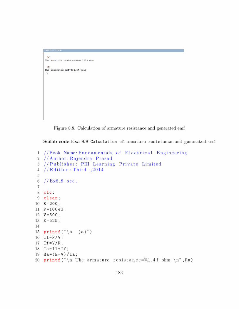
Figure 8.8: Calculation of armature resistance and generated emf
Scilab code Exa 8.8 Calculation of armature resistance and generated emf
1 // Book Name : Fundamentals o f E l e c t r i c a l E n g i n e e r i n g2 // Author : Rajendra Prasad3 // P u b l i s h e r : PHI Lea rn ing P r i v a t e L imi ted4 // E d i t i o n : Third ,20145
6 // Ex8 8 . s c e .7
8 clc;
9 clear;
10 R=200;
11 P=100e3;
12 V=500;
13 E=525;
14
15 printf(”\n ( a ) ”)16 Il=P/V;
17 If=V/R;
18 Ia=Il+If;
19 Ra=(E-V)/Ia;
20 printf(”\n The armature r e s i s t a n c e=%1 . 4 f ohm \n”,Ra)
183

Figure 8.9: Calculation of armature generated voltage
21
22 printf(”\n ( b ) ”)23 P=60e3;
24 V=520;
25 Il=P/V;
26 If=V/R;
27 Ia=Il+If;
28 E=V+(Ia*Ra);
29 printf(”\n The g e n e r a t e d emf=%3 . 2 f v o l t ”,E)
Scilab code Exa 8.9 Calculation of armature generated voltage
1 // Book Name : Fundamentals o f E l e c t r i c a l E n g i n e e r i n g2 // Author : Rajendra Prasad3 // P u b l i s h e r : PHI Lea rn ing P r i v a t e L imi ted4 // E d i t i o n : Third ,20145
184
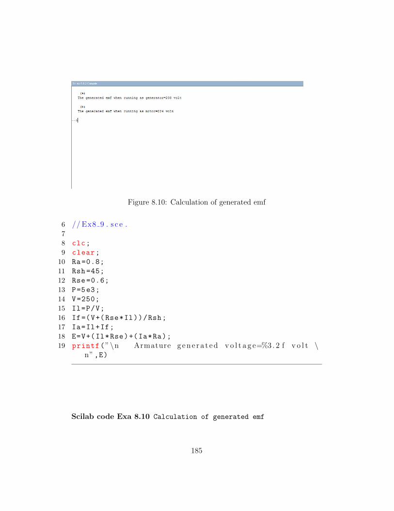
Figure 8.10: Calculation of generated emf
6 // Ex8 9 . s c e .7
8 clc;
9 clear;
10 Ra=0.8;
11 Rsh =45;
12 Rse =0.6;
13 P=5e3;
14 V=250;
15 Il=P/V;
16 If=(V+(Rse*Il))/Rsh;
17 Ia=Il+If;
18 E=V+(Il*Rse)+(Ia*Ra);
19 printf(”\n Armature g e n e r a t e d v o l t a g e=%3 . 2 f v o l t \n”,E)
Scilab code Exa 8.10 Calculation of generated emf
185

1 // Book Name : Fundamentals o f E l e c t r i c a l E n g i n e e r i n g2 // Author : Rajendra Prasad3 // P u b l i s h e r : PHI Lea rn ing P r i v a t e L imi ted4 // E d i t i o n : Third ,20145
6 // Ex8 10 . s c e .7
8 clc;
9 clear;
10 Ra=0.1;
11
12 printf(”\n ( a ) ”)13 Ia=80;
14 V=230;
15 E=V+(Ia*Ra);
16 printf(”\n The g e n e r a t e d emf when runn ing asg e n e r a t o r=%3 . 0 f v o l t \n”,E)
17
18 printf(”\n ( b ) ”)19 Ia=60;
20 V=230;
21 E=V-(Ia*Ra);
22 printf(”\n The g e n e r a t e d emf when runn ing as motor=%3 . 0 f v o l t \n”,E)
Scilab code Exa 8.11 Calculation of motor speed
1 // Book Name : Fundamentals o f E l e c t r i c a l E n g i n e e r i n g2 // Author : Rajendra Prasad3 // P u b l i s h e r : PHI Lea rn ing P r i v a t e L imi ted4 // E d i t i o n : Third ,20145
6 // Ex8 11 . s c e .
186

Figure 8.11: Calculation of motor speed
7
8 clc;
9 clear;
10 V1=440;
11 V2=220;
12 Ia=50;
13 Ra=0.3;
14 a=2;
15 p=2;
16 Z=850;
17 phi_1 =0.025;
18 phi_2 =0.02;
19
20 E=V1 -(Ia*Ra);
21 n1=(E*a)/(2*Z*p*phi_1);
22 N1=n1*60;
23 n1_by_n2 =(V1*phi_2)/(V2*phi_1);
24 n2=n1/( n1_by_n2);
25 N2=n2*60;
26 printf(”\n Motor Speed : \ t N1=%d r . p .m \ t N2=%d r .
187

Figure 8.12: Calculation of motor speed and gross torque developed
p .m \n”,N1 ,N2)
Scilab code Exa 8.12 Calculation of motor speed and gross torque developed
1 // Book Name : Fundamentals o f E l e c t r i c a l E n g i n e e r i n g2 // Author : Rajendra Prasad3 // P u b l i s h e r : PHI Lea rn ing P r i v a t e L imi ted4 // E d i t i o n : Third ,20145
6 // Ex8 12 . s c e .7
8 clc;
9 clear;
10 V=480;
11 Ia=110;
12 Ra=0.2;
13 Z=864;
14 phi =0.05;
188

Figure 8.13: Calculation of motor speed and current and speed regulation
15 a=6;
16 p=3;
17
18 printf(”\n ( a ) ”)19 E=V-(Ia*Ra);
20 n=(E*a)/(2*Z*p*phi);
21 N=(n*60);
22 printf(”\n Speed=%d r . p .m \n”,N)23
24 printf(”\n ( b ) ”)25 Pm=E*Ia;
26 T=Pm/(2* %pi*n);
27 printf(”\n Gross t o r q u e deve l oped i n the armature=%d Nm \n”,T)
Scilab code Exa 8.13 Calculation of motor speed and current and speed regulation
189

1 // Book Name : Fundamentals o f E l e c t r i c a l E n g i n e e r i n g2 // Author : Rajendra Prasad3 // P u b l i s h e r : PHI Lea rn ing P r i v a t e L imi ted4 // E d i t i o n : Third ,20145
6 // Ex8 13 . s c e .7
8 clc;
9 clear;
10 Il=2;
11 Z=864;
12 If=0.6;
13 V=220;
14 Ra=0.8;
15 a=2;
16 p=2;
17 phi =5.4e-3;
18 T=25;
19
20 Ia=Il-If;
21 E1=V-(Ia*Ra);
22 n1=(E1*a)/(2*Z*phi*p);
23 N1=n1*60;
24 printf(”\n Motor speed at no l oad=%4 . 0 f r . p .m \n”,N1)
25
26 Ia=(T*a*%pi)/(p*phi*Z);
27 Il=Ia+If;
28 printf(”\n Motor c u r r e n t at f u l l l o ad to r q u e=%2 . 3 fA \n”,Il)
29 E2=V-(Ia*Ra);
30 n2=(E2*a)/(2*Z*phi*p);
31 N2=n2*60;
32 printf(”\n Motor speed at f u l l l o ad=%4 . 0 f r . p .m \n”,N2)
33
34 speed_reg =((N1-N2)/N2)*100;
35 printf(”\n Speed r e g u l a t i o n=%1 . 3 f p e r c e n t a g e ”,
190

Figure 8.14: Calculation of current and kW input of the motor
speed_reg)
36 // There i s a e r r o r i n the r e g u l a t i o n c a l c u l a t i o n i nthe book
37 //The book answer 9 . 9 5% i s wrong
Scilab code Exa 8.14 Calculation of current and kW input of the motor
1 // Book Name : Fundamentals o f E l e c t r i c a l E n g i n e e r i n g2 // Author : Rajendra Prasad3 // P u b l i s h e r : PHI Lea rn ing P r i v a t e L imi ted4 // E d i t i o n : Third ,20145
6 // Ex8 14 . s c e .7
8 clc;
9 clear;
191

10 N=600;
11 V=500;
12 Il=32;
13 Ra=0.4;
14 Rf=250;
15
16 printf(”\n ( a ) ”)17 P=(V*Il)/1e3;
18 N1=450;
19 Ia=Il -(V/Rf);
20 k_phi=(V-(Ia*Ra))/N;
21 R=(V-( k_phi*N1))/Ia-Ra;
22 printf(”\n Input power at 600 r . p .m=%d kW \n”,P)23 printf(”\n Armature c u r r e n t Ia=%d A \n”,Ia)24 printf(”\n R=%1. 2 f ohm \n”,R)25
26 printf(”\n ( b ) ”)27 //To i n c r e a s e the speed the f i e l d c o n t r o l i s used .28 If1_by_If =0.856;
29 If=Il-Ia;
30 If1=If1_by_If*If;
31 Rf1=V/If1;
32 R=Rf1 -Rf;
33 Ia1=Ia/If1_by_If;
34 Il=Ia1+If1;
35 Pi=(V*Il)/1e3;
36 printf(”\n New armature c u r r e n t Ia=%d A \n”,Ia1)37 printf(”\n New Input power=%2 . 1 f kW”,Pi)
Scilab code Exa 8.15 Calculation of external resistance and electric braking torque
1 // Book Name : Fundamentals o f E l e c t r i c a l E n g i n e e r i n g2 // Author : Rajendra Prasad
192

Figure 8.15: Calculation of external resistance and electric braking torque
3 // P u b l i s h e r : PHI Lea rn ing P r i v a t e L imi ted4 // E d i t i o n : Third ,20145
6 // Ex8 15 . s c e .7
8 clc;
9 clear;
10 P_in_HP =37.5;
11 V=220;
12 N=535;
13 Ra =0.086;
14 Ia1 =140;
15 I=200;
16
17 E=V-(Ia1*Ra);
18 R=(V+E)/I;
19 R_ext=R-Ra;
20 P=( P_in_HP)*736;
21 omega =(2* %pi*N)/60;
22 FL_T=P/omega;
23 initial_braking_T=FL_T*(I/Ia1);
24 Ia2=(V+(E/2))/R;
25 halfspeed_braking_T=FL_T*(Ia2/Ia1);
193
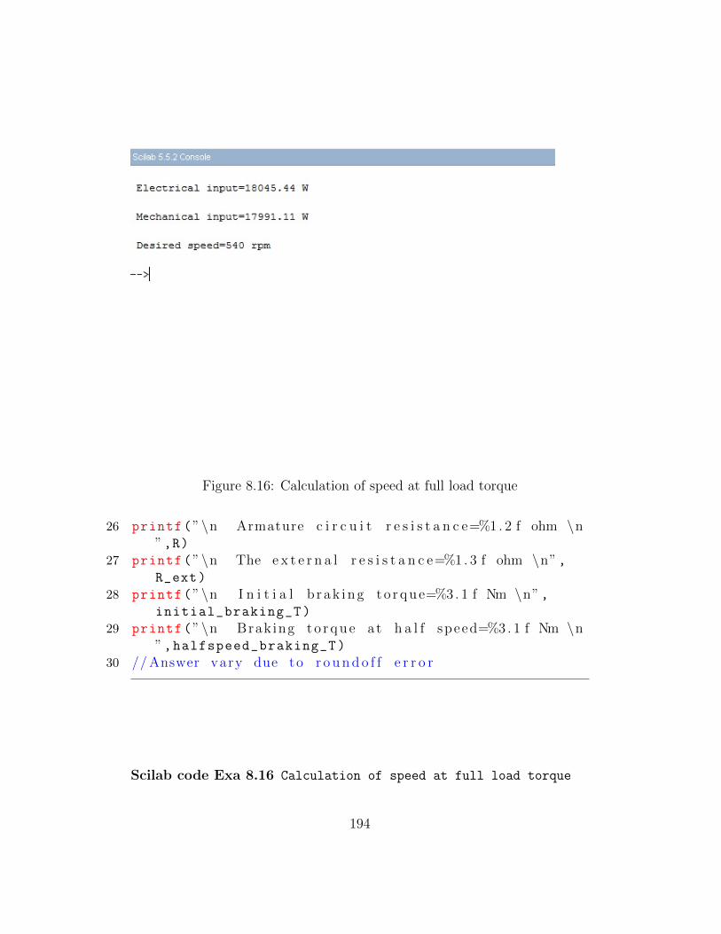
Figure 8.16: Calculation of speed at full load torque
26 printf(”\n Armature c i r c u i t r e s i s t a n c e=%1 . 2 f ohm \n”,R)
27 printf(”\n The e x t e r n a l r e s i s t a n c e=%1 . 3 f ohm \n”,R_ext)
28 printf(”\n I n i t i a l b rak ing t o r q ue=%3 . 1 f Nm \n”,initial_braking_T)
29 printf(”\n Brak ing t o r q u e at h a l f speed=%3 . 1 f Nm \n”,halfspeed_braking_T)
30 // Answer vary due to r o u n d o f f e r r o r
Scilab code Exa 8.16 Calculation of speed at full load torque
194

1 // Book Name : Fundamentals o f E l e c t r i c a l E n g i n e e r i n g2 // Author : Rajendra Prasad3 // P u b l i s h e r : PHI Lea rn ing P r i v a t e L imi ted4 // E d i t i o n : Third ,20145
6 // Ex8 16 . s c e .7
8 clc;
9 clear;
10 P_in_HP =20;
11 P=( P_in_HP)*736;
12 N=450;
13 Ra =0.18;
14 Rf =0.12;
15 R=8.7+ Ra+Rf;
16 omega =(2* %pi*N)/60;
17 Tf=P/omega;
18
19 //The v o l t a g e deve l oped f o r 450 rpm i s 289 v o l twhich i s taken from the curve
20 E=289;
21 P_not=(E*E)/R;
22 Pi=(2* %pi*N*Tf)/60;
23
24 //The mechan i ca l i nput i s g r e a t e r than e l e c t r i c a loutput , so the motor speed i n c r e a s e s
25 //The v o l t a g e deve l oped f o r 550 rpm i s 403 v o l twhich i s taken from the curve
26 N=550;
27 E=403;
28 P_not=(E*E)/R;
29 Pi=(2* %pi*N*Tf)/60;
30
31 printf(”\n E l e c t r i c a l i nput=%5 . 2 f W \n”,P_not)32 printf(”\n Mechan ica l i nput=%5 . 2 f W \n”,Pi)33 if Pi<P_not then
34 N1=540;
35 else
195

Figure 8.17: Calculation of efficiency of generator at full load and half load
36 N1 >N
37 end
38 printf(”\n D e s i r e d speed=%d rpm \n”,N1)39 // Answer vary dueto r o u n d o f f e r r o r40 // s i n c e mechan i ca l i nput i s l e s s than e l e c t r i c a l
output the motor cannot a t t a i n a speed as 550 rpm41 // So the speed i s 540 rpm which i s o b t a i n e d u s i n g
t r i a l and e r r o r method
Scilab code Exa 8.17 Calculation of efficiency of generator at full load and half load
1 // Book Name : Fundamentals o f E l e c t r i c a l E n g i n e e r i n g2 // Author : Rajendra Prasad3 // P u b l i s h e r : PHI Lea rn ing P r i v a t e L imi ted4 // E d i t i o n : Third ,20145
6 // Ex8 17 . s c e .7
8 clc;
196

9 clear;
10 P=100e3;
11 V=460;
12 It=9.8;
13 If=2.7;
14 R=0.11;
15
16 printf(”\n ( a ) ”)17 I=(P/2)/V;
18 Ia=I+If;
19 Wa=Ia^2*R;
20 Wsh=V*If;
21 Ian=It -If;
22 W_not=V*Ian;
23 NL_armature_loss=Ian^2*R;
24 other_loss=W_not -NL_armature_loss; //o t h e r l o s s e s i n c l u d e i r on , f r i c t i o n , windage l o s s e s
25 T_loss_HL=Wa+Wsh+other_loss;
26 Pi_HL=(P/2)+T_loss_HL;
27 efficiency =((P/2)/Pi_HL)*100;
28 printf(”\n E f f i c i e n c y o f the g e n e r a t o r at h a l f l o ad=%2 . 1 f p e r c e n t a g e \n”,efficiency)
29
30 printf(”\n ( b ) ”)31 I=P/V;
32 Ia=I+If;
33 Wa=Ia^2*R;
34 Wsh=V*If;
35 Ian=It -If;
36 W_not=V*Ian;
37 NL_armature_loss=Ian^2*R;
38 other_loss=W_not -NL_armature_loss; //o t h e r l o s s e s i n c l u d e i r on , f r i c t i o n , windage l o s s e s
39 T_loss_FL=Wa+Wsh+other_loss;
40 Pi_FL=P+T_loss_FL;
41 efficiency =(P/Pi_FL)*100;
42 printf(”\n E f f i c i e n c y o f the g e n e r a t o r at f u l l l o ad=%2 . 2 f p e r c e n t a g e \n”,efficiency)
197

Figure 8.18: Calculation of efficiency of the generator
Scilab code Exa 8.18 Calculation of efficiency of the generator
1 // Book Name : Fundamentals o f E l e c t r i c a l E n g i n e e r i n g2 // Author : Rajendra Prasad3 // P u b l i s h e r : PHI Lea rn ing P r i v a t e L imi ted4 // E d i t i o n : Third ,20145
6 // Ex8 18 . s c e .7
8 clc;
9 clear;
10 P=1000 e3;
11 V=500;
12 I1 =2000;
13 I2=400;
14 Ig=21; // shunt f i e l d c u r r e n t o f g e n e r a t o r15 Im=17; // shunt f i e l d c u r r e n t o f motor
198
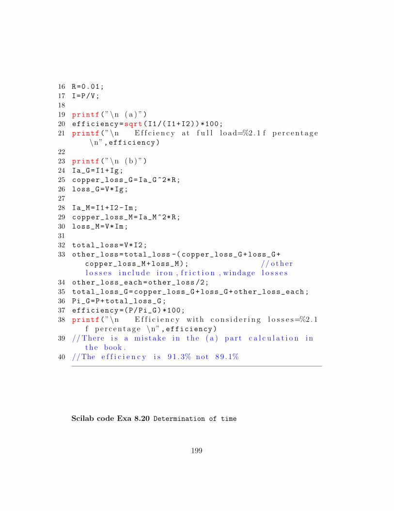
16 R=0.01;
17 I=P/V;
18
19 printf(”\n ( a ) ”)20 efficiency=sqrt(I1/(I1+I2))*100;
21 printf(”\n E f f c i e n c y at f u l l l o ad=%2 . 1 f p e r c e n t a g e\n”,efficiency)
22
23 printf(”\n ( b ) ”)24 Ia_G=I1+Ig;
25 copper_loss_G=Ia_G ^2*R;
26 loss_G=V*Ig;
27
28 Ia_M=I1+I2-Im;
29 copper_loss_M=Ia_M ^2*R;
30 loss_M=V*Im;
31
32 total_loss=V*I2;
33 other_loss=total_loss -( copper_loss_G+loss_G+
copper_loss_M+loss_M); // o t h e rl o s s e s i n c l u d e i r on , f r i c t i o n , windage l o s s e s
34 other_loss_each=other_loss /2;
35 total_loss_G=copper_loss_G+loss_G+other_loss_each;
36 Pi_G=P+total_loss_G;
37 efficiency =(P/Pi_G)*100;
38 printf(”\n E f f i c i e n c y with c o n s i d e r i n g l o s s e s=%2 . 1f p e r c e n t a g e \n”,efficiency)
39 // There i s a mi s take i n the ( a ) pa r t c a l c u l a t i o n i nthe book .
40 //The e f f i c i e n c y i s 9 1 . 3% not 8 9 . 1%
Scilab code Exa 8.20 Determination of time
199

Figure 8.19: Determination of time
1 // Book Name : Fundamentals o f E l e c t r i c a l E n g i n e e r i n g2 // Author : Rajendra Prasad3 // P u b l i s h e r : PHI Lea rn ing P r i v a t e L imi ted4 // E d i t i o n : Third ,20145
6 // Ex8 20 ( c ) . s c e .7
8 clc;
9 clear;
10 Ra=35;
11 J=6e-5;
12 K=0.325;
13
14 T=(J*Ra)/K^2;
15 t=-T*log (1 -0.98); // (1 −0 .98) =0.0216 printf(”\n Time f o r the motor to run with 2
p e r c e n t a g e o f i t s f i n a l speed=%1 . 3 f s e c \n”,t)
200

Chapter 9
Synchronous Machines
Scilab code Exa 9.1 Calculation of distribution factor
1 // Book Name : Fundamentals o f E l e c t r i c a l E n g i n e e r i n g2 // Author : Rajendra Prasad3 // P u b l i s h e r : PHI Lea rn ing P r i v a t e L imi ted4 // E d i t i o n : Third ,20145
6 // Ex9 1 . s c e .7
8 clc;
9 clear;
10 slots =24;
11 pole =4;
12
13 printf(”\n ( a ) ”)14 //when a l l s l o t s a r e wound15 m=slots/pole;
16 alpha =180/m;
17 Kd=sind(m*alpha /2)/(m*sind(alpha /2));
18 printf(”\n D i s t r i b u t i o n f a c t o r when a l l s l o t s a r ewound=%1 . 3 f ”,Kd)
201

Figure 9.1: Calculation of distribution factor
19
20 printf(”\n ( b ) ”)21 // on ly 4 a d j a c e n t s l o t s a r e wound22 m=4;
23 Kd=sind(m*alpha /2)/(m*sind(alpha /2));
24 printf(”\n D i s t r i b u t i o n f a c t o r when on ly f o u r s l o t sper p o l e a r e wound=%1 . 3 f ”,Kd)
Scilab code Exa 9.2 Calculation of number of poles and flux per pole
1 // Book Name : Fundamentals o f E l e c t r i c a l E n g i n e e r i n g2 // Author : Rajendra Prasad3 // P u b l i s h e r : PHI Lea rn ing P r i v a t e L imi ted4 // E d i t i o n : Third ,20145
6 // Ex9 2 . s c e7
202
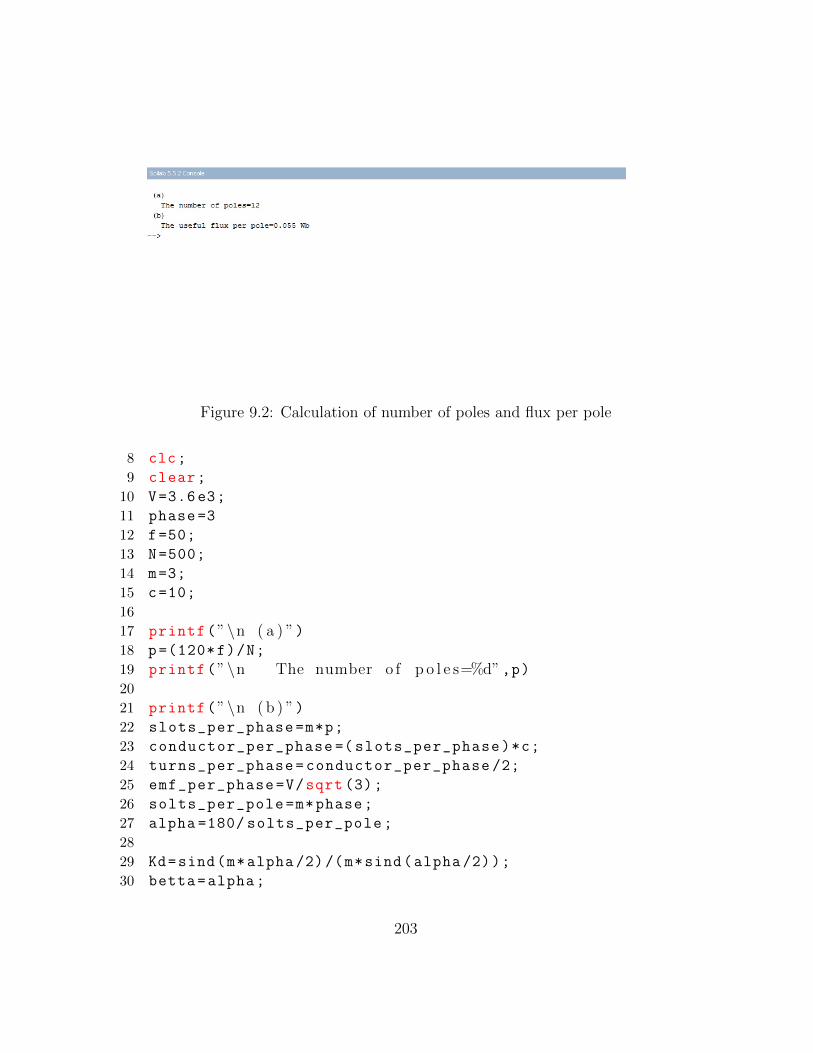
Figure 9.2: Calculation of number of poles and flux per pole
8 clc;
9 clear;
10 V=3.6e3;
11 phase=3
12 f=50;
13 N=500;
14 m=3;
15 c=10;
16
17 printf(”\n ( a ) ”)18 p=(120*f)/N;
19 printf(”\n The number o f p o l e s=%d”,p)20
21 printf(”\n ( b ) ”)22 slots_per_phase=m*p;
23 conductor_per_phase =( slots_per_phase)*c;
24 turns_per_phase=conductor_per_phase /2;
25 emf_per_phase=V/sqrt (3);
26 solts_per_pole=m*phase;
27 alpha =180/ solts_per_pole;
28
29 Kd=sind(m*alpha /2)/(m*sind(alpha /2));
30 betta=alpha;
203

Figure 9.3: Determination of short circuit ratio and synchronous reactance
31 Kp=cosd(betta /2);
32 phi=emf_per_phase /(4.44*f*Kd*Kp*turns_per_phase);
33 printf(”\n The u s e f u l f l u x per p o l e=%1 . 3 f Wb”,phi)
Scilab code Exa 9.3 Determination of short circuit ratio and synchronous reactance
1 // Book Name : Fundamentals o f E l e c t r i c a l E n g i n e e r i n g2 // Author : Rajendra Prasad3 // P u b l i s h e r : PHI Lea rn ing P r i v a t e L imi ted4 // E d i t i o n : Third ,20145
6 // Ex9 3 . s c e7
8 clc;
9 clear;
10 P=45e3;
11 E=220;
12 phase =3;
13 p=6;
204

14 f=50;
15
16 I=P/(E*sqrt (3));
17 //From SCC , the e x c i t a t i o n c u r r e n t i s ,18 Isc1 =118.1;
19 If=2.2;
20 // For t h i s I f , the c o r r e s p o n d i n g l i n e v o l t a g e fromthe a i r gap l i n e i s ,
21 V1=202;
22 I1=1.0;
23 Vph=V1/sqrt (3);
24 Xs_unsat=Vph/Isc1; // Unsaturated r e a c t a n c ei n ohm
25 V=V1/E;
26 Xs_unsat_pu=V/I1; // Unsaturatedr e a c t a n c e i n per u n i t
27 printf(”\n Unsaturated v a l u e o f synchronousr e a c t a n c e =\t %1 . 4 f ohm \ t %1 . 3 f p . u \n”,Xs_unsat ,Xs_unsat_pu)
28
29 // For 220 v o l t from f i g u r e ,30 If=2.9;
31 Isc2 =157;
32 Vph=E/sqrt (3);
33 Xs_sat=Vph/Isc2;
34 Xs_sat_pu=I1/(Isc2/Isc1);
35 printf(”\n S a t u r a t e d v a l u e o f synchronous r e a c t a n c e=\t %1 . 3 f ohm \ t %1 . 3 f p . u \n”,Xs_sat ,Xs_sat_pu)
36
37 Ie2 =2.9;
38 Ie1 =2.2;
39 SCR=Ie2/Ie1;
40 printf(”\n Short c i r c u i t r a t i o=%1 . 2 f \n”,SCR)
205

Figure 9.4: Calculation of leakage reactance and field current
Scilab code Exa 9.4 Calculation of leakage reactance and field current
1 // Book Name : Fundamentals o f E l e c t r i c a l E n g i n e e r i n g2 // Author : Rajendra Prasad3 // P u b l i s h e r : PHI Lea rn ing P r i v a t e L imi ted4 // E d i t i o n : Third ,20145
6 // Ex9 4 . s c e .7
8 clc;
9 clear;
10 //From f i g u r e 9 . 2 611 EG=25;
12 P=45e3;
13 E=220;
14 I=P/(E*sqrt (3));
15 Xl=EG/(sqrt (3)*I);
16 printf(”\n Leakage r e a c t a n c e=%1 . 4 f ohm \n”,Xl)17
18 //From f i g 9 . 2 6 armature r e a c t i o n amphere i s e q u a lto the f i e l d c u r r e n t
206
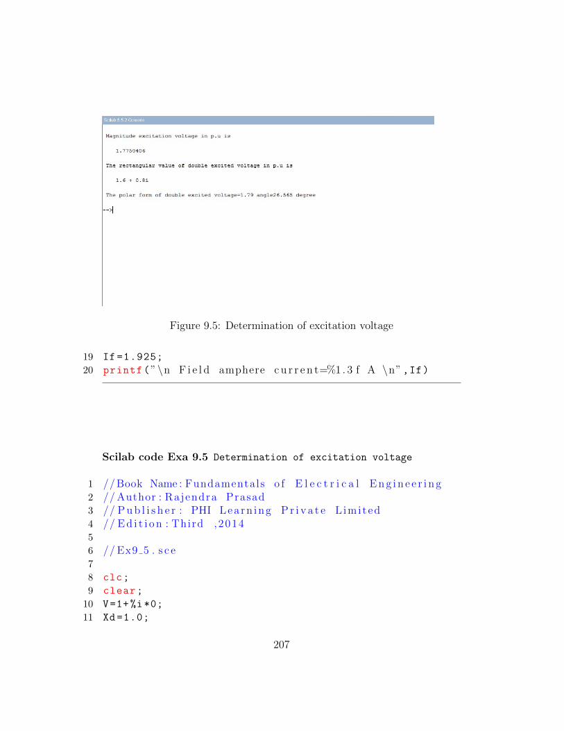
Figure 9.5: Determination of excitation voltage
19 If =1.925;
20 printf(”\n F i e l d amphere c u r r e n t=%1 . 3 f A \n”,If)
Scilab code Exa 9.5 Determination of excitation voltage
1 // Book Name : Fundamentals o f E l e c t r i c a l E n g i n e e r i n g2 // Author : Rajendra Prasad3 // P u b l i s h e r : PHI Lea rn ing P r i v a t e L imi ted4 // E d i t i o n : Third ,20145
6 // Ex9 5 . s c e7
8 clc;
9 clear;
10 V=1+%i*0;
11 Xd=1.0;
207

12 Xq=0.6;
13 pf=0.8;
14 theta=acosd(pf);
15 Ia1=pf -%i*sind(acosd(pf));
16 Ia=1.0; // phase magnitude o f I a17
18 tan_del =(Ia*Xq*cosd(theta))/(V+(Ia*Xq*sind(theta)));
19 del=atand(real(tan_del));
20 Ef_dash =((V+(Ia*Xq*sind(theta)))^2+(Ia*Xq*cosd(theta
))^2) ^(1/2);
21
22 Ef=real(Ef_dash)+(Ia*sind(theta+del)*(Xd-Xq));
23 disp(Ef, ’ Magnitude e x c i t a t i o n v o l t a g e i n p . u i s ’ )24
25 Ef_double_dash=V*(1+%i*0)+%i*(( cosd(theta)-%i*sind(
theta))*Xd);
26 disp(Ef_double_dash , ’ The r e c t a n g u l a r v a l u e o f doub lee x c i t e d v o l t a g e i n p . u i s ’ )
27
28 Ef_double_dash_mag=sqrt(real(Ef_double_dash)^2+ imag(
Ef_double_dash)^2);
29 Ef_double_dash_ang=atand(imag(Ef_double_dash)/real(
Ef_double_dash));
30 printf(”\n The p o l a r form o f doub l e e x c i t e d v o l t a g e=%1 . 2 f angle%2 . 3 f d e g r e e \n”,Ef_double_dash_mag ,Ef_double_dash_ang)
Scilab code Exa 9.6 Calculation of voltage regulation
1 // Book Name : Fundamentals o f E l e c t r i c a l E n g i n e e r i n g2 // Author : Rajendra Prasad3 // P u b l i s h e r : PHI Lea rn ing P r i v a t e L imi ted4 // E d i t i o n : Third ,2014
208
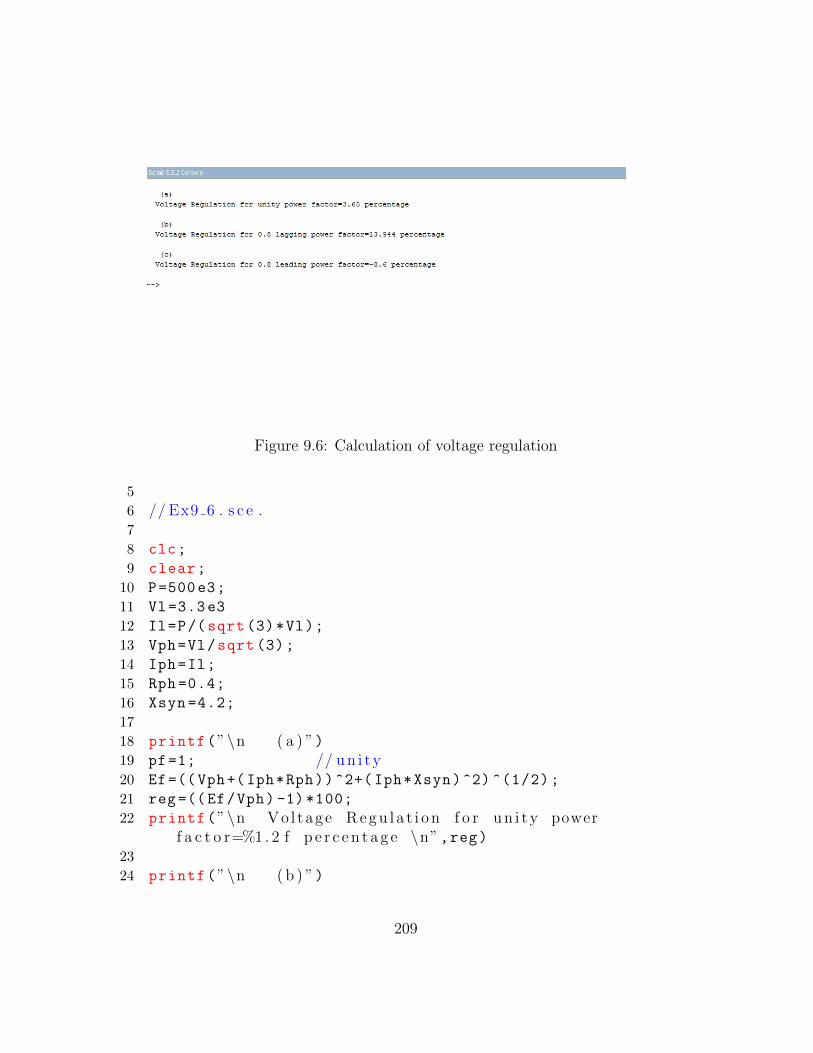
Figure 9.6: Calculation of voltage regulation
5
6 // Ex9 6 . s c e .7
8 clc;
9 clear;
10 P=500e3;
11 Vl=3.3e3
12 Il=P/(sqrt (3)*Vl);
13 Vph=Vl/sqrt (3);
14 Iph=Il;
15 Rph =0.4;
16 Xsyn =4.2;
17
18 printf(”\n ( a ) ”)19 pf=1; // u n i t y20 Ef=((Vph+(Iph*Rph))^2+( Iph*Xsyn)^2) ^(1/2);
21 reg =((Ef/Vph) -1)*100;
22 printf(”\n Vo l tage R e g u l a t i o n f o r u n i t y powerf a c t o r=%1 . 2 f p e r c e n t a g e \n”,reg)
23
24 printf(”\n ( b ) ”)
209

25 pf=0.8; // l a g g i n g26 theta=acosd(pf);
27 Ef=((Vph+(Iph*Rph*cosd(theta))+(Iph*Xsyn*sind(theta)
))^2+(( Iph*Xsyn*cosd(theta)) -(Iph*Rph*sind(theta)
))^2) ^(1/2);
28 reg =((Ef/Vph) -1)*100;
29 printf(”\n Vo l tage R e g u l a t i o n f o r 0 . 8 l a g g i n g powerf a c t o r=%2 . 3 f p e r c e n t a g e \n”,reg)
30
31 printf(”\n ( c ) ”)32 pf=0.8; // l e a d i n g33 theta=acosd(pf);
34 Ef=((Vph+(Iph*Rph*cosd(theta))-(Iph*Xsyn*sind(theta)
))^2+(( Iph*Xsyn*cosd(theta))+(Iph*Rph*sind(theta)
))^2) ^(1/2);
35 reg =((Ef/Vph) -1)*100;
36 printf(”\n Vo l tage R e g u l a t i o n f o r 0 . 8 l e a d i n g powerf a c t o r=%1 . 1 f p e r c e n t a g e \n”,reg)
Scilab code Exa 9.7 Calculation of voltage regulation
1 // Book Name : Fundamentals o f E l e c t r i c a l E n g i n e e r i n g2 // Author : Rajendra Prasad3 // P u b l i s h e r : PHI Lea rn ing P r i v a t e L imi ted4 // E d i t i o n : Third ,20145
6 // Ex9 7 . s c e .7
8 clc;
9 clear;
10 // input data a r e taken from example 9 . 511 V=1+%i*0;
12 Xd=1.0;
210

Figure 9.7: Calculation of voltage regulation
13 Xq=0.6;
14 pf=0.8;
15 theta=acosd(pf);
16 Ia1=pf -%i*sind(acosd(pf));
17 Ia=1.0; // phase magnitude o f I a18
19 printf(”\n ( a ) ”)20 // l a g g i n g power f a c t o r21 tan_del =(Ia*Xq*cosd(theta))/(V+(Ia*Xq*sind(theta)));
22 del=atand(real(tan_del));
23 Ef_dash =((V+(Ia*Xq*sind(theta)))^2+(Ia*Xq*cosd(theta
))^2) ^(1/2);
24 Ef=real(Ef_dash)+(Ia*sind(theta+del)*(Xd-Xq));
25 reg =((Ef -V)/1.0) *100;
26 printf(”\n Vo l tage R e g u l a t i o n f o r 0 . 8 l a g g i n g powerf a c t o r=%d p e r c e n t a g e \n”,reg)
27
28 printf(”\n ( b ) ”)29 tan_del =(Ia*Xq*cosd(theta))/(V-(Ia*Xq*sind(theta)));
30 del=atand(real(tan_del));
31 Ef=((V-(Ia*Xq*sind(theta)))^2+(Ia*Xq*cosd(theta))^2)
211

Figure 9.8: Determination of capacity of the condenser
^(1/2);
32 reg =((Ef -V)/1.0) *100;
33 printf(”\n Vo l tage R e g u l a t i o n f o r 0 . 8 l e a d i n g powerf a c t o r=%2 . 0 f p e r c e n t a g e ”,reg)
Scilab code Exa 9.8 Determination of capacity of the condenser
1 // Book Name : Fundamentals o f E l e c t r i c a l E n g i n e e r i n g2 // Author : Rajendra Prasad3 // P u b l i s h e r : PHI Lea rn ing P r i v a t e L imi ted4 // E d i t i o n : Third ,20145
6 // Ex9 8 . s c e .7
212

Figure 9.9: Determination of capacity of the synchronous condenser
8 clc;
9 clear;
10 VI1 =10e6;
11 phi1=acosd (0.75);
12 phip=acosd (0.9);
13 phic=90- asind (7/100); // g i v e n l o s s i s 7%o f KVA output
14 KVAc=VI1 *((( sind(phi1)*cosd(phip))-(cosd(phi1)*sind(
phip)))/(( sind(phic)*cosd(phip))+(cosd(phic)*sind
(phip))))*1e-3;
15 MVAc=KVAc*1e-3;
16 printf(”\n The c a p a c i t y o f the synchronousco nde n s e r= %1 . 2 f MVA”,MVAc)
Scilab code Exa 9.9 Determination of capacity of the synchronous condenser
1 // Book Name : Fundamentals o f E l e c t r i c a l E n g i n e e r i n g2 // Author : Rajendra Prasad
213

Figure 9.10: Determination of line current and power factor
3 // P u b l i s h e r : PHI Lea rn ing P r i v a t e L imi ted4 // E d i t i o n : Third ,20145
6 // Ex9 9 . s c e .7
8 // input data a r e taken from example 9 . 89 clc;
10 clear;
11 VI1 =10e6;
12 pf1 =0.75;
13 pfc=cosd(90-asind (7/100));
14 KVAc=VI1*(( sqrt(1-pf1 ^2))/(sqrt(1-pfc^2)))*1e-3;
15 MVAc=KVAc*1e-3;
16 printf(”\n The c a p a c i t y o f synchronous co nde n s e rwhich i s d e s i r e d to r a i s e the power f a c t o r tou n i t y=%1 . 2 f MVA”,MVAc);
214

Scilab code Exa 9.10 Determination of line current and power factor
1 // Book Name : Fundamentals o f E l e c t r i c a l E n g i n e e r i n g2 // Author : Rajendra Prasad3 // P u b l i s h e r : PHI Lea rn ing P r i v a t e L imi ted4 // E d i t i o n : Third ,20145
6 // Ex9 10 . s c e .7
8 clc;
9 clear;
10 Pl=1e6;
11 Pd=360; // d e v e l o p i n g power12 Pi=600e3;
13 Vl =6600;
14 pf=0.8;
15 Pin =800e3;
16 theta=acosd(pf);
17 Il=Pl/(Vl*sqrt (3));
18 Ps=(Pd *746) /0.9; // 1HP=746 watt ande f f i c i e n c y i s assumed 90% ( i . e 0 . 9 )
19 phi_s=acosd(Ps/Pi);
20 Is=Pi/(Vl*sqrt (3));
21 lag_reactive_crt_load=Il*sind(theta);
22 lead_reacitve_crt_motor=lag_reactive_crt_load*sind(
phi_s);
23 lag_reactive_crt_result=lag_reactive_crt_load -
lead_reacitve_crt_motor;
24 resultant_active_crt =(Il*pf)+( lag_reactive_crt_load*
cosd(phi_s));
25
26 resultant_line_crt=sqrt(resultant_active_crt ^2+
lag_reactive_crt_result ^2);
27 printf(”\n R e s u l t a n t l i n e c u r r e n t=%2 . 2 f A \n”,
215

Figure 9.11: Determination of increase in additional loss and decrease in linecurrent and final line current
resultant_line_crt);
28
29 final_power_factor=resultant_active_crt/
resultant_line_crt;
30 printf(”\n F i n a l power f a c t o r=%1 . 0 f \n”,final_power_factor);
31
32 increase_of_crt =( resultant_line_crt -Il)*100/Il;
33 printf(”\n The i n c r e a s e o f c u r r e n t=%2 . 1 f p e r c e n t a g e\n”,increase_of_crt)
34
35 increase_power_trans =((Pin+Ps)-Pin)*100/ Pin;
36 printf(”\n The i n c r e a s e o f power t r a n s m i t t e d=%2 . 1 fp e r c e n t a g e \n”,increase_power_trans)
Scilab code Exa 9.11 Determination of increase in additional loss and decrease in line current and final line current
216

1 // Book Name : Fundamentals o f E l e c t r i c a l E n g i n e e r i n g2 // Author : Rajendra Prasad3 // P u b l i s h e r : PHI Lea rn ing P r i v a t e L imi ted4 // E d i t i o n : Third ,20145
6 // Ex9 11 . s c e7
8 clc;
9 clear;
10 //The input data a r e taken from the p r e v i o u s example9 . 1 0
11
12 Pl=1e6;
13 Pd=360; // d e v e l o p i n g power14 Pi=600e3;
15 Vl =6600;
16 pf=0.1;
17 pf1 =0.8;
18 Pin =800e3;
19 theta=acosd(pf);
20 Il=Pl/(Vl*sqrt (3));
21 Ps=(Pd *746) /0.9; // 1HP=746 watt ande f f i c i e n c y i s assumed 90% ( i . e 0 . 9 )
22 phi_s=acosd(Ps/Pi);
23 Is=Pi/(Vl*sqrt (3));
24 lag_reactive_crt_motor =52.5;
25 lead_reacitve_crt_motor=lag_reactive_crt_motor*sind(
acosd(pf));
26 active_crt=lag_reactive_crt_motor*pf;
27 lag_reactive_crt_result=lag_reactive_crt_motor -
lead_reacitve_crt_motor;
28 resultant_active_crt =(Il*pf1)+( active_crt);
29
30 resultant_line_crt=sqrt(resultant_active_crt ^2+
lag_reactive_crt_result ^2);
31 printf(”\n R e s u l t a n t l i n e c u r r e n t= %2 . 3 f A \n”,resultant_line_crt);
32
217

33 pf=resultant_active_crt/resultant_line_crt;
34 printf(”\n Power f a c t o r= %1 . 0 f \n”,pf)35
36 increase_of_crt =(Il-resultant_active_crt)*100/ Il;
37 printf(”\n The i n c r e a s e o f c u r r e n t= %2 . 0 fp e r c e n t a g e \n”,increase_of_crt)
38
39 increase_power_trans =(Pi*pf)*100/ Pin;
40 printf(”\n The i n c r e a s e o f power t r a n s m i t t e d= %2 . 0 fp e r c e n t a g e ”,increase_power_trans)
218

Chapter 10
Three Phase Induction Motor
Scilab code Exa 10.1 Calculation of synchronous speed and rotor speed and rotor frequency
1 // Book Name : Fundamentals o f E l e c t r i c a l E n g i n e e r i n g2 // Author : Rajendra Prasad3 // P u b l i s h e r : PHI Lea rn ing P r i v a t e L imi ted4 // E d i t i o n : Third ,20145
6 // Ex10 1 . s c e7
8 clc;
9 clear;
10 f=50;
11 p=4;
12
13 printf(”\n ( a ) ”)14 Ns =(120*f)/p;
15 printf(”\n Synchronous speed=%d r . p .m \n”,Ns)16
17 printf(”\n ( b ) ”)18 s=0.04;
19 N=Ns -(s*Ns);
219
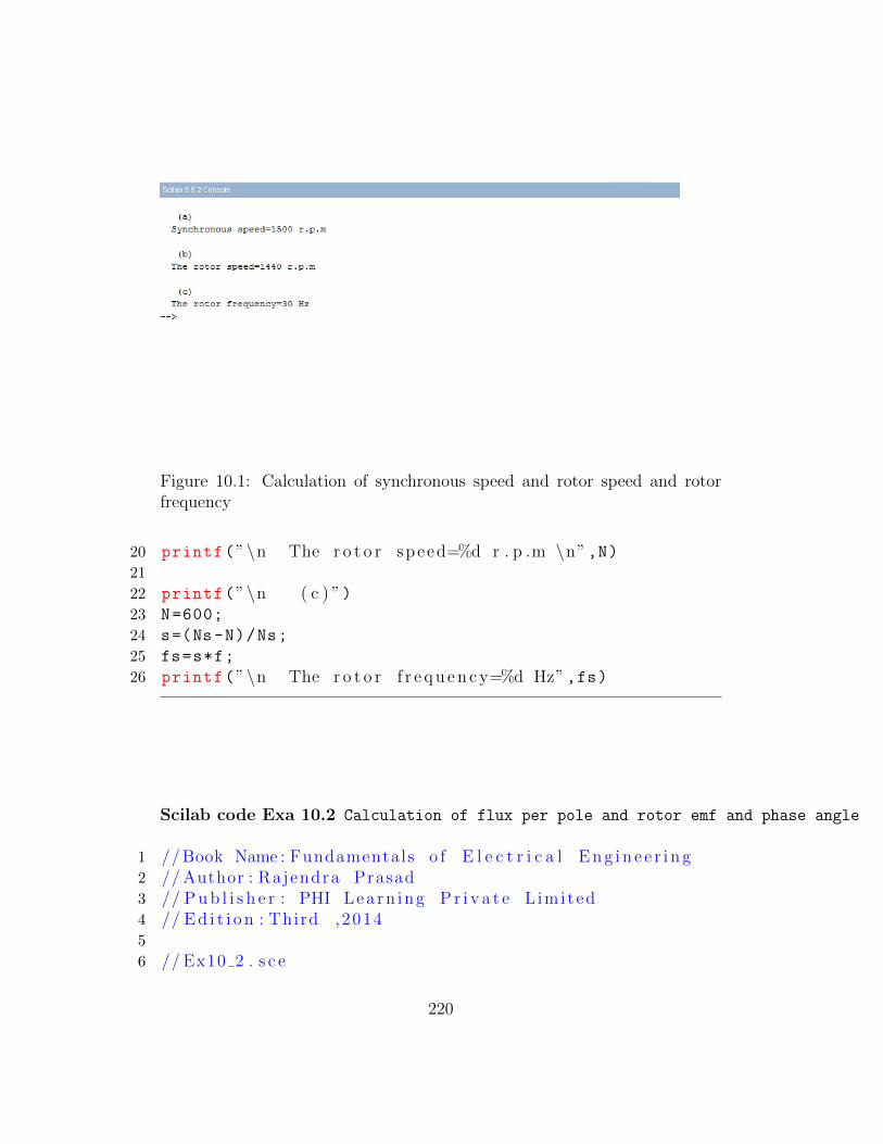
Figure 10.1: Calculation of synchronous speed and rotor speed and rotorfrequency
20 printf(”\n The r o t o r speed=%d r . p .m \n”,N)21
22 printf(”\n ( c ) ”)23 N=600;
24 s=(Ns-N)/Ns;
25 fs=s*f;
26 printf(”\n The r o t o r f r e q u e n c y=%d Hz”,fs)
Scilab code Exa 10.2 Calculation of flux per pole and rotor emf and phase angle
1 // Book Name : Fundamentals o f E l e c t r i c a l E n g i n e e r i n g2 // Author : Rajendra Prasad3 // P u b l i s h e r : PHI Lea rn ing P r i v a t e L imi ted4 // E d i t i o n : Third ,20145
6 // Ex10 2 . s c e
220

Figure 10.2: Calculation of flux per pole and rotor emf and phase angle
7
8 clc;
9 clear;
10 T1=120;
11 T2=24;
12 R2 =0.013;
13 X2 =0.048;
14 V=400;
15 kd =0.96;
16 kp=1.0;
17 f=50;
18
19 printf(”\n ( a ) ”)20 phi=V/(4.44* kd*kp*f*T1);
21 printf(”\n The f l u x per p o l e=%1 . 6 f Wb \n”,phi)22
23 printf(”\n ( b ) ”)24 E2 =4.44* kd*kp*phi*f*T2;
25 printf(”\n The r o t o r emf induced at s t a n d s t i l l onopen c i r c u i t=%d V \n”,E2)
221

26
27 printf(”\n ( c ) ”)28 s=0.04;
29 Er=s*E2;
30 printf(”\n Rotor emf at a s l i p=%1 . 1 f V”,Er)31 Ir=Er/sqrt(R2^2+(s*X2)^2);
32 printf(”\n The r o t o r c u r r e n t=%3 . 2 f A \n”,Ir)33
34 printf(”\n ( d ) \ t ( i ) ”)35 s=0.04;
36 phir=atand(s*(X2/R2));
37 printf(”\n The phase d i f f e r e n c e between r o t o r emfand c u r r e n t f o r 4 p e r c e n t a g e s l i p=%2 . 2 f d e g r e e ”,phir)
38 printf(”\n\ t ( i i ) ”)39 s=1;
40 phir=atand(s*(X2/R2));
41 printf(”\n The phase d i f f e r e n c e between r o t o r emfand c u r r e n t f o r 100 p e r c e n t a g e s l i p=%2 . 2 f d e g r e e ”,phir)
Scilab code Exa 10.3 Calculation of output power and mechanical power developed and rotor copper loss and efficiency
1 // Book Name : Fundamentals o f E l e c t r i c a l E n g i n e e r i n g2 // Author : Rajendra Prasad3 // P u b l i s h e r : PHI Lea rn ing P r i v a t e L imi ted4 // E d i t i o n : Third ,20145
6 // Ex10 3 . s c e7
8 clc;
9 clear;
10 Pin =40; // power i n kW
222

Figure 10.3: Calculation of output power and mechanical power developedand rotor copper loss and efficiency
11 Ps=1.5; // power i n kW12 Ns=100; // speed p e r c e n t a g e v a l u e13 N=40; // speed p e r c e n t a g e v a l u e14 power_loss =0.8; // power i n kW15
16 printf(”\n ( a ) ”)17 rotor_input_power=Pin -Ps;
18 s=0.04;
19 rotor_copper_loss=s*rotor_input_power;
20 mec_power_developed=rotor_input_power -
rotor_copper_loss;
21 printf(”\n Mechan ica l power deve l oped by the r o t o r=%2 . 2 f kW”,mec_power_developed)
22 printf(”\n Rotor copper l o s s=%2 . 2 f kW \n”,rotor_copper_loss)
23
24 printf(”\n ( b ) ”)25 motor_output_power=mec_power_developed -power_loss;
26 printf(”\n Output o f the motor=%2 . 2 f kW \n”,motor_output_power)
223

27
28 printf(”\n ( c ) ”)29 motor_efficiency =( motor_output_power/Pin)*100;
30 printf(”\n The motor e f f i c i e n c y=%2 . 1 f p e r c e n t a g e \n”,motor_efficiency)
31
32 printf(”\n ( d ) ”)33 new_slip =(Ns -N)/Ns;
34 total_rotor_copper_loss=new_slip*rotor_input_power;
35 printf(”\n Tota l r o t o r copper l o s s when speedreduced to 40 p e r c e n t a g e o f synchronous speed=%2 . 1f kW \n”,total_rotor_copper_loss)
36
37 printf(”\n ( e ) ”)38 total_rotor_loss=total_rotor_copper_loss+power_loss;
39 motor_output_power=rotor_input_power -
total_rotor_loss;
40 motor_efficiency =( motor_output_power/Pin)*100;
41 printf(”\n E f f i c i e n c y o f motor when speed reducedto 40 p e r c e n t a g e o f synchronous speed=%2 . 1 fp e r c e n t a g e ”,motor_efficiency)
Scilab code Exa 10.4 Determination of synchronous speed and slip and maximum torque and rotor frequency
1 // Book Name : Fundamentals o f E l e c t r i c a l E n g i n e e r i n g2 // Author : Rajendra Prasad3 // P u b l i s h e r : PHI Lea rn ing P r i v a t e L imi ted4 // E d i t i o n : Third ,20145
6 // Ex10 4 . s c e7
8 clc;
9 clear;
224

Figure 10.4: Determination of synchronous speed and slip and maximumtorque and rotor frequency
10
11 f=50;
12 p=4;
13 V=400;
14 E2=190;
15 R1=0.5;
16 X1=2.5;
17 R2 =0.06;
18 X2=0.3;
19
20 printf(”\n ( a ) ”)21 Ns =(120*f)/p;
22 printf(”\n Synchronous speed=%d r . p .m \n”,Ns)23
24 printf(”\n ( b ) ”)25 s=(R2/X2)*100;
26 printf(”\n S l i p at which maximum to r q u e o c c u r s=%dp e r c e n t a g e \n”,s)
27
28 printf(”\n ( c ) ”)29 E=E2/sqrt (3);
225

30 Ir=(s*E)/(sqrt (2)*R2*100);
31 pf=1/ sqrt (2);
32 Pi=sqrt (3)*E2*Ir*pf;
33 P0=(1-s/100)*Pi;
34 Tm=Pi/(2* %pi*Ns/60);
35 printf(”\n Maximum Torque=%3 . 2 f synchronous watt \n”,Tm)
36
37 printf(”\n ( d ) ”)38 Tfl =(1/2)*Tm;
39 // ( 2 / 1 ) =(R2ˆ2+ s f ˆ2∗X2ˆ2) /(2∗X2∗R2∗ s f )40 //From t h i s e q u a t i o n we ge t s f ˆ2−0.8∗ s f +0.04=0;41 a=1;
42 b=-0.8; //a , b , c a r e c o e f f i c i e n t v a l u e s taken from theabove second o r d e r e q u a t i o n
43 c=0.04;
44 sf=(-b-sqrt(b^2 -(4*a*c)))/(2*a);
45 sf_percentage=sf *100;
46 Nf=Ns*(1-sf);
47 Pf=2*%pi*(Nf/60)*Tfl;
48 printf(”\n F u l l l o ad t o r q u e=%3 . 2 f synchronous watt ”,Tfl)
49 printf(”\n F u l l l o ad s l i p=%1 . 1 f p e r c e n t a g e ”,sf_percentage)
50 printf(”\n Speed at f u l l l o ad=%d r . p .m”,Nf)51 printf(”\n Power output=%2 . 2 f kW \n”,Pf /1000)52 // Answer vary dueto round o f f e r r o r53
54 printf(”\n ( e ) ”)55 f_at_fullload=sf*f;
56 printf(”\n The r o t o r f r e q u e n c y at f u l l l o ad=%1 . 1 fHz”,f_at_fullload)
226

Figure 10.5: Calculation of number of poles and slip and rotor copper loss
Scilab code Exa 10.5 Calculation of number of poles and slip and rotor copper loss
1 // Book Name : Fundamentals o f E l e c t r i c a l E n g i n e e r i n g2 // Author : Rajendra Prasad3 // P u b l i s h e r : PHI Lea rn ing P r i v a t e L imi ted4 // E d i t i o n : Third ,20145
6 // Ex10 5 . s c e7
8 clc;
9 clear;
10 f=50;
11 N=285;
12 Ns=300; // which i s near the v a l u e o f N as s l i p l i e sb/w 0 . 0 3 to 0 . 0 5
13
14 printf(”\n ( a ) ”)15 p=(120*f)/Ns;
16 printf(”\n Number o f p o l e s=%d \n”,p)17
18 printf(”\n ( b ) ”)
227

Figure 10.6: Determination of starting torque
19 s=(Ns-N)/Ns;
20 s_percentage=s*100;
21 printf(”\n S l i p at f u l l l o ad=%d p e r c e n t a g e \n”,s_percentage)
22
23 printf(”\n ( c ) ”)24 // s l i p i s p r o p o r t i o n a l to r o t o r r e s i s t a n c e25 s=2* s_percentage;
26 printf(”\n S l i p at f u l l l o ad i f r o t o r r e s i s t a n c e i sdoubled=%d p e r c e n t a g e \n”,s)
27
28 printf(”\n ( d ) ”)29 // copper l o s s=I ˆ2∗R; so copper l o s s d o u b l e s i f r o t o r
r e s i s t a n c e d o u b l e s30 Pcu =280;
31 Pcu_new =2*Pcu;
32 printf(”\n The new v a l u e o f r o t o r copper l o s s=%dwatt \n”,Pcu_new)
Scilab code Exa 10.6 Determination of starting torque
228
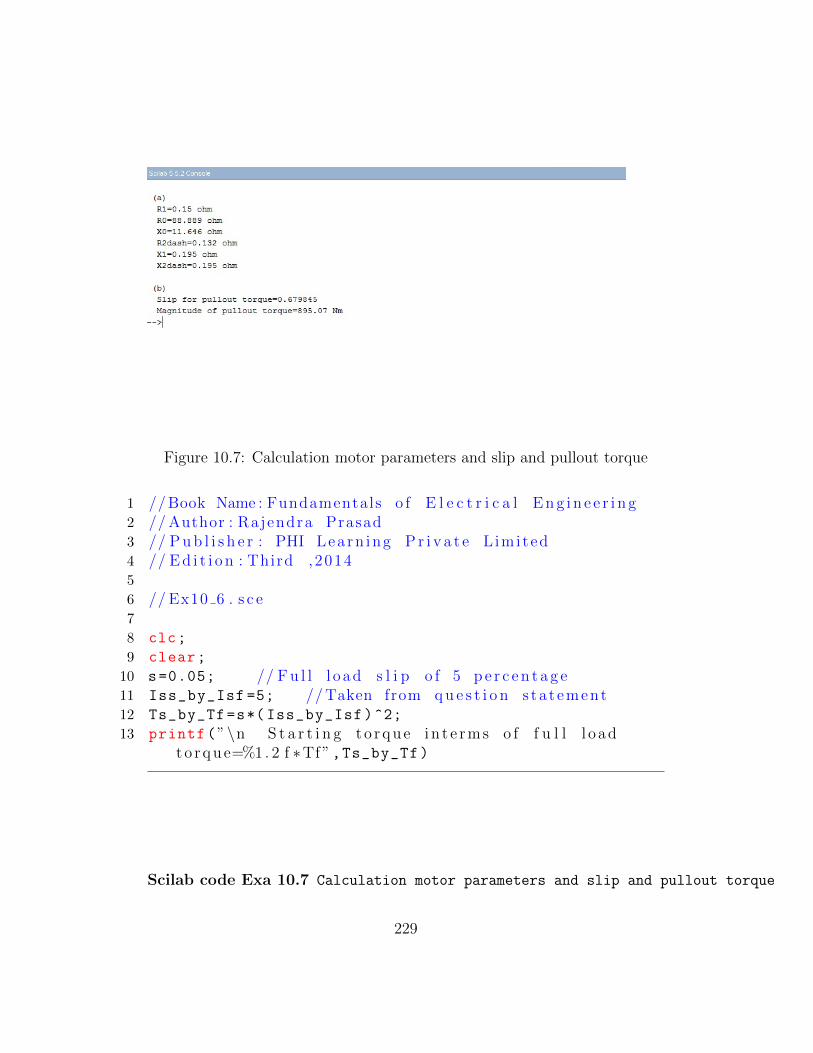
Figure 10.7: Calculation motor parameters and slip and pullout torque
1 // Book Name : Fundamentals o f E l e c t r i c a l E n g i n e e r i n g2 // Author : Rajendra Prasad3 // P u b l i s h e r : PHI Lea rn ing P r i v a t e L imi ted4 // E d i t i o n : Third ,20145
6 // Ex10 6 . s c e7
8 clc;
9 clear;
10 s=0.05; // F u l l l o ad s l i p o f 5 p e r c e n t a g e11 Iss_by_Isf =5; // Taken from q u e s t i o n s ta t ement12 Ts_by_Tf=s*( Iss_by_Isf)^2;
13 printf(”\n S t a r t i n g to r q u e i n t e r m s o f f u l l l o adt o rq u e=%1 . 2 f ∗Tf ”,Ts_by_Tf)
Scilab code Exa 10.7 Calculation motor parameters and slip and pullout torque
229

1 // Book Name : Fundamentals o f E l e c t r i c a l E n g i n e e r i n g2 // Author : Rajendra Prasad3 // P u b l i s h e r : PHI Lea rn ing P r i v a t e L imi ted4 // E d i t i o n : Third ,20145
6 // Ex10 7 . s c e7
8 clc;
9 clear;
10 Vl_not =400; //No load v o l t a g e i n v o l t11 Vl_sc =50; // Blocked r o t o r v o l t a g e i n v o l t12 I_not =20; //No load c u r r e n t i n Ampere13 Isc =60; // Blocked r o t o r c u r r n e t i n Ampere14 W1_not =5e3; // watt meter r e a d i n g s f o r no l oad
t e s t i n watt15 W2_not =-3.2e3; // watt meter r e a d i n g s f o r no l oad
t e s t i n watt16 Wsc1 =2.3e3; // watt meter r e a d i n g s f o r b l o cked
r o t o r t e s t i n watt17 Wsc2 =0.75e3; // watt meter r e a d i n g s f o r b l o cked
r o t o r t e s t i n watt18 Vdc =18; // dc v o l t a g e i n v o l t19 Idc =60; // dc l i n e c u r r e n t i n Ampere20
21 printf(”\n ( a ) ”)22 R1=(Vdc/Idc)/2;
23 printf(”\n R1=%1 . 2 f ohm”,R1)24 P_not=W1_not+W2_not;
25 V_not=Vl_not/sqrt (3);
26 cos_phi_not=P_not /(3* V_not*I_not);
27 R_not=V_not /( I_not*cos_phi_not);
28 printf(”\n R0=%2 . 3 f ohm”,R_not)29 // R not answer vary dueto round o f f e r r o r i n v no t
and c o s p h i n o t30 X_not=V_not /( I_not*sqrt(1- cos_phi_not ^2));
31 printf(”\n X0=%2 . 3 f ohm”,X_not)32 Psc=Wsc1+Wsc2;
33 Vsc=Vl_sc/sqrt (3);
230

34 cos_phi_sc=Psc /(3* Vsc*Isc);
35 R2_dash =((Vsc/Isc)*cos_phi_sc)-R1;
36 printf(”\n R2dash=%1 . 3 f ohm”,R2_dash)37 X1=((Vsc/Isc)*sqrt(1- cos_phi_sc ^2))/2;
38 printf(”\n X1=%1 . 3 f ohm”,X1)39 X2_dash=X1;
40 printf(”\n X2dash=%1 . 3 f ohm \n”,X2_dash)41
42 printf(”\n ( b ) ”)43 ns=25;
44 s=R2_dash/X2_dash; // S l i p f o r maximum t o rq u e45 pf_max =1/ sqrt (2);
46 Ps=(3* V_not ^2)/sqrt((R1+R2_dash/s)^2+(2* X1)^2);
47 Pc=(3* V_not ^2*(R1+R2_dash))/((R1+R2_dash/s)^2+(2* X1)
^2); // S t a t o r copper l o s s i n kw48 Pin=Ps -Pc;
49 T=Pin /(2* %pi*ns);
50 printf(”\n S l i p f o r p u l l o u t t o r q ue=%g”,s)51 printf(”\n Magnitude o f p u l l o u t t o r q u e=%3 . 2 f Nm”,T)52 // There i s a mi s take i n the book s o l u t i o n i n pa r t ( b
)53 //The c a l c u l a t e d Ps v a l u e i s wrong54 // Hence T answer vary
Scilab code Exa 10.9 Determination ratio of starting current to full load current
1 // Book Name : Fundamentals o f E l e c t r i c a l E n g i n e e r i n g2 // Author : Rajendra Prasad3 // P u b l i s h e r : PHI Lea rn ing P r i v a t e L imi ted4 // E d i t i o n : Third ,20145
6 // Ex10 9 . s c e7
231

Figure 10.8: Determination ratio of starting current to full load current
8 clc;
9 clear;
10 P_in_HP =10;
11 eta =0.9;
12 pf=0.8;
13 Vl=400;
14 Vsc =160;
15 Isc =7.2;
16 P_in_watt=P_in_HP *735.5;
17 If=P_in_watt /(sqrt (3)*Vl*pf*eta);
18 Isc_400=Isc*Vl/Vsc;
19 Ist=Isc_400 /3;
20 Ist_by_If=Ist/If;
21 printf(”\n The r a t i o v a l u e o f s t a r t i n g c u r r e n t tof u l l l o ad c u r r e n t=%1 . 3 f ”,Ist_by_If)
Scilab code Exa 10.10 Calculation of starting torque and starting current
1 // Book Name : Fundamentals o f E l e c t r i c a l E n g i n e e r i n g2 // Author : Rajendra Prasad
232

Figure 10.9: Calculation of starting torque and starting current
3 // P u b l i s h e r : PHI Lea rn ing P r i v a t e L imi ted4 // E d i t i o n : Third ,20145
6 // EX10 10 . s c e .7 clc;
8 clear;
9 sf =0.04;
10 If =37.5;
11 f=50;
12 p=4;
13 V=400;
14 P_in_HP =25;
15 z=2.8;
16 P_in_watt=P_in_HP *735.5;
17 Nf =((120*f)/p)*(1-sf);
18 nf=Nf/60;
19 Tf=P_in_watt /(2* %pi*nf);
20 Isc_phase=V/z;
21 Isc=sqrt (3)*Isc_phase;
233

22
23 printf(”\n ( i ) Using D i r e c t s w i t c h i n g ”)24 Ist=Isc;
25 printf(”\n \ t The s t a r t i n g c u r r e n t=%3 . 2 f A”,Ist)26 Tst=(Isc/If)^2*sf*Tf;
27 printf(”\n \ t The s t a r t i n g t o r qu e=%3 . 1 f Nm \n”,Tst)28
29 printf(”\n ( i i ) Using S ta r d e l t a c o n n e c t o r ”)30 Ist =(1/3)*Isc;
31 printf(”\n \ t The s t a r t i n g c u r r e n t=%3 . 2 f A”,Ist)32 Tst =(1/3) *(Isc/If)^2*sf*Tf;
33 printf(”\n \ t The s t a r t i n g t o r qu e=%3 . 1 f Nm \n”,Tst)34
35 printf(”\n ( i i i ) Us ing auto t r a n s f o r m e r ”)36 k=0.7;
37 Ist=k^2*Isc;
38 printf(”\n \ t The s t a r t i n g c u r r e n t=%3 . 2 f A”,Ist)39 Tst=k^2*( Isc/If)^2*sf*Tf;
40 printf(”\n \ t The s t a r t i n g t o r qu e=%3 . 1 f Nm \n”,Tst)
Scilab code Exa 10.11 Calculation of plugging torque
1 // Book Name : Fundamentals o f E l e c t r i c a l E n g i n e e r i n g2 // Author : Rajendra Prasad3 // P u b l i s h e r : PHI Lea rn ing P r i v a t e L imi ted4 // E d i t i o n : Third ,20145
6 // Ex10 11 . s c e7
8 clc;
9 clear;
10
11
234

Figure 10.10: Calculation of plugging torque
12 P_in_HP =25;
13 s=0.04;
14 p=4;
15 f=50;
16 Ns =(120*f)/p;
17 ns=Ns/60;
18 nf=(1-s)*ns;
19 P_in_watt=P_in_HP *735.5;
20 Tf=P_in_watt /(2* %pi*nf);
21 sf=s;
22 sp=2-s; //At the t ime o f p l u g g i n g the s l i pi s 200%
23 a=4;
24 X2_by_R2=a;
25 Tp=(sp/sf)*((1+( sf^2* X2_by_R2 ^2))/(1+(sp^2* X2_by_R2
^2)))*Tf;
26 printf(”\n Plugg ing t o r q u e at f u l l l o ad=%2 . 1 f Nm”,Tp)
235

Figure 10.11: Calculation of external resistance
Scilab code Exa 10.12 Calculation of external resistance
1 // Book Name : Fundamentals o f E l e c t r i c a l E n g i n e e r i n g2 // Author : Rajendra Prasad3 // P u b l i s h e r : PHI Lea rn ing P r i v a t e L imi ted4 // E d i t i o n : Third ,20145
6 // Ex10 12 . s c e7
8 clc;
9 clear;
10 p=4;
11 f=50;
12 R2 =0.25;
13 N1 =1425;
14 N2 =1275;
15
16 Ns =(120*f)/p;
17 s1=(Ns-N1)/Ns;
236
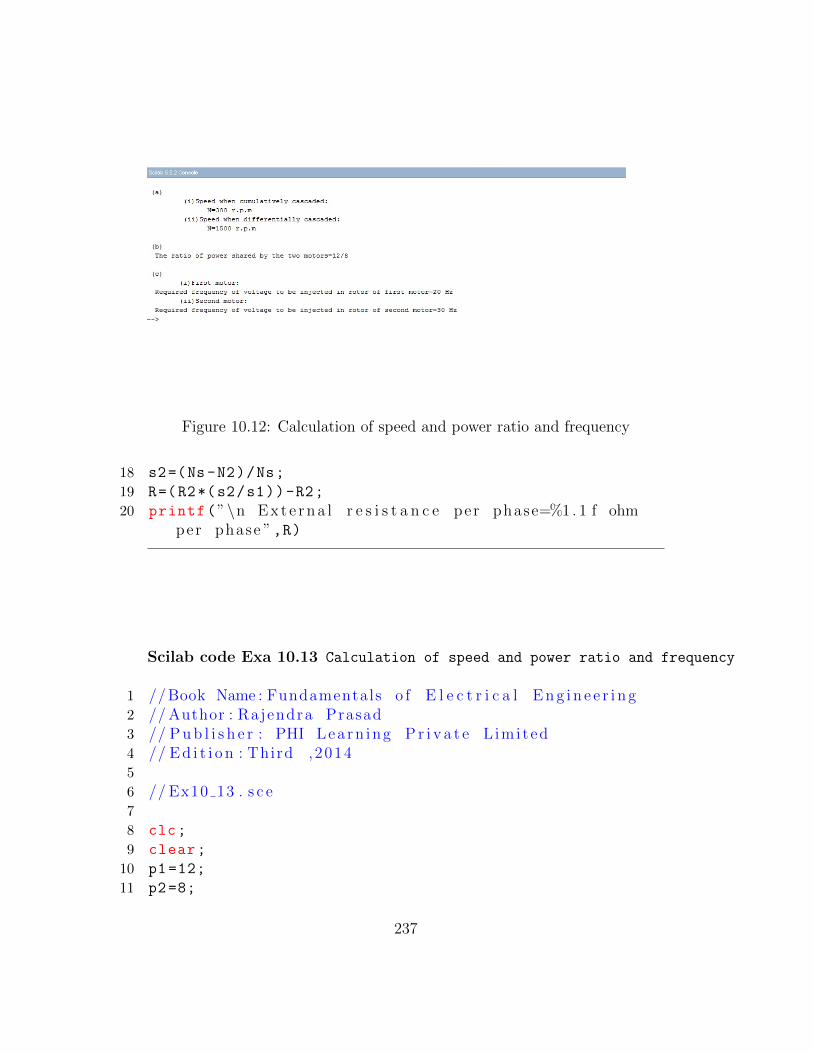
Figure 10.12: Calculation of speed and power ratio and frequency
18 s2=(Ns-N2)/Ns;
19 R=(R2*(s2/s1))-R2;
20 printf(”\n E x t e r n a l r e s i s t a n c e per phase=%1 . 1 f ohmper phase ”,R)
Scilab code Exa 10.13 Calculation of speed and power ratio and frequency
1 // Book Name : Fundamentals o f E l e c t r i c a l E n g i n e e r i n g2 // Author : Rajendra Prasad3 // P u b l i s h e r : PHI Lea rn ing P r i v a t e L imi ted4 // E d i t i o n : Third ,20145
6 // Ex10 13 . s c e7
8 clc;
9 clear;
10 p1=12;
11 p2=8;
237

12 f=50;
13 printf(”\n ( a ) ”)14 printf(”\n \ t ( i ) Speed when c u m u l a t i v e l y ca s caded : ”)15 N1 =(120*f)/(p1+p2);
16 printf(”\n \ t N=%d r . p .m”,N1)17 printf(”\n \ t ( i i ) Speed when d i f f e r e n t i a l l y ca s caded
: ”)18 N2 =(120*f)/(p1-p2);
19 printf(”\n \ t N=%d r . p .m \n”,N2)20
21 printf(”\n ( b ) ”)22 printf(”\n The r a t i o o f power sha r ed by the two
motors=%d/%d \n”,p1 ,p2)23
24 printf(”\n ( c ) ”)25 printf(”\n \ t ( i ) F i r s t motor : ”)26 Ns1 =(120*f)/p1;
27 s1=(Ns1 -N1)/Ns1;
28 sf1=s1*f;
29 printf(”\n Requ i red f r e q u e n c y o f v o l t a g e to bei n j e c t e d i n r o t o r o f f i r s t motor=%d Hz”,sf1)
30 printf(”\n \ t ( i i ) Second motor : ”)31 Ns2 =(120*f)/p2;
32 s2=(Ns2 -N1)/Ns2;
33 sf2=s2*f;
34 printf(”\n Requ i red f r e q u e n c y o f v o l t a g e to bei n j e c t e d i n r o t o r o f s econd motor=%d Hz”,sf2)
238

Chapter 11
Special Purpose ElectricalMachines
Scilab code Exa 11.1 Determination of motor parameters and stator current and power factor and speed and torque
1 // Book Name : Fundamentals o f E l e c t r i c a l E n g i n e e r i n g2 // Author : Rajendra Prasad3 // P u b l i s h e r : PHI Lea rn ing P r i v a t e L imi ted4 // E d i t i o n : Third ,20145
6 // Ex11 1 . s c e7
8 clc;
9 clear;
10 V_not =220;
11 I_not =4;
12 W_not =100;
13 Vsc =110;
14 Isc =10;
15 Wsc =400;
16 p=6;
17 V=220;
239

Figure 11.1: Determination of motor parameters and stator current andpower factor and speed and torque
18 f=50;
19
20 printf(”\n ( a ) ”)21 r1=(Wsc/Isc ^2)/2;
22 x1=sqrt((Vsc/Isc)^2-(2*r1)^2) /2;
23 r2_dash=r1;
24 x2_dash=x1;
25 phi_not=acosd(W_not /( V_not*I_not));
26 V_not_dash=V_not -(( I_not *(cosd(phi_not)-%i*sind(
phi_not)))*((r1+r2_dash /4)+%i*(x1+x2_dash /2)));
27 Wi=W_not -(I_not ^2*(r1+r2_dash /4));
28 R_not_by_2 =( V_not_dash ^2)/Wi;
29 Y_not=(I_not)/( V_not_dash *2);
30 B_not=sqrt ((2* Y_not)^2-(1/ R_not_by_2)^2) /2;
31 X_not_by_2 =1/(2* B_not);
32 printf(”\n Parameters o f the motor : ”)33 printf(”\n \ t r1=r2dash=%d ohm”,r1)34 printf(”\n \ t x1=x2dash=%1 . 3 f ohm”,x1)
240
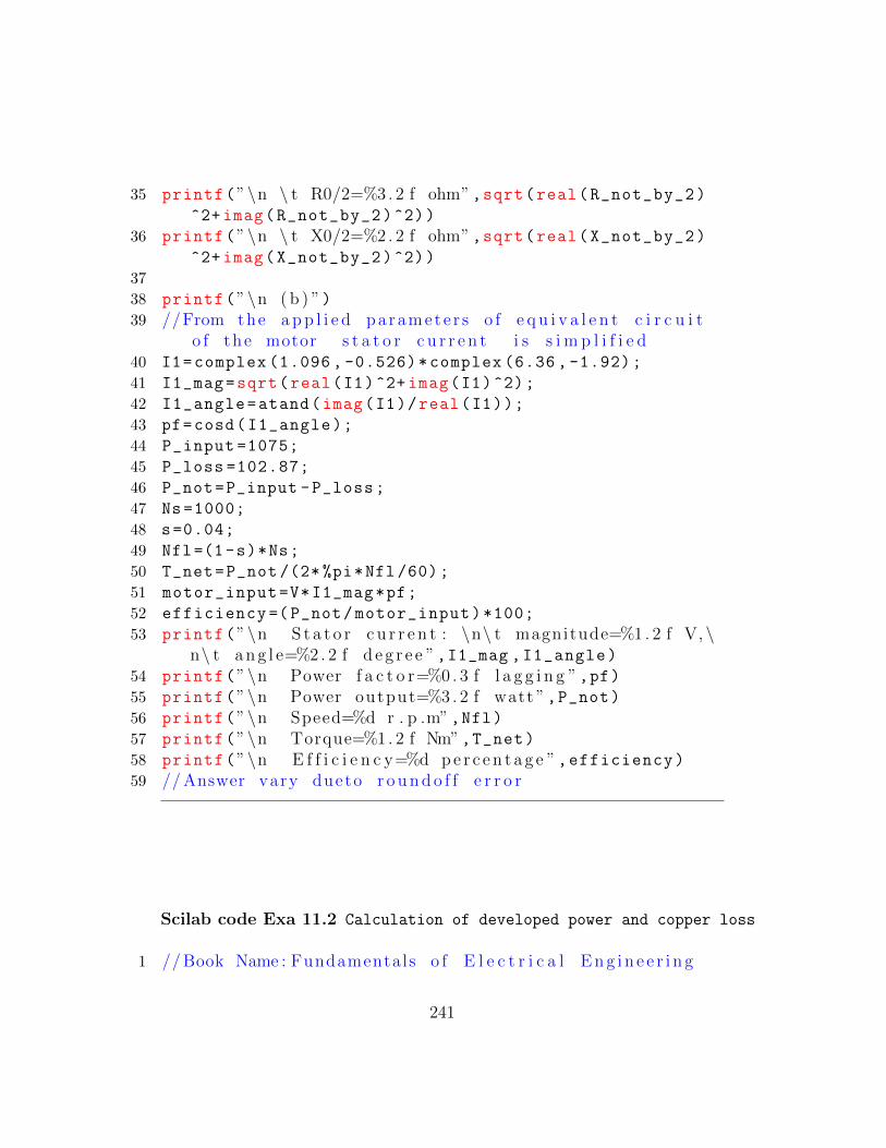
35 printf(”\n \ t R0/2=%3 . 2 f ohm”,sqrt(real(R_not_by_2)^2+ imag(R_not_by_2)^2))
36 printf(”\n \ t X0/2=%2 . 2 f ohm”,sqrt(real(X_not_by_2)^2+ imag(X_not_by_2)^2))
37
38 printf(”\n ( b ) ”)39 //From the a p p l i e d paramete r s o f e q u i v a l e n t c i r c u i t
o f the motor s t a t o r c u r r e n t i s s i m p l i f i e d40 I1=complex (1.096 , -0.526)*complex (6.36 , -1.92);
41 I1_mag=sqrt(real(I1)^2+ imag(I1)^2);
42 I1_angle=atand(imag(I1)/real(I1));
43 pf=cosd(I1_angle);
44 P_input =1075;
45 P_loss =102.87;
46 P_not=P_input -P_loss;
47 Ns =1000;
48 s=0.04;
49 Nfl=(1-s)*Ns;
50 T_net=P_not /(2* %pi*Nfl /60);
51 motor_input=V*I1_mag*pf;
52 efficiency =(P_not/motor_input)*100;
53 printf(”\n S t a t o r c u r r e n t : \n\ t magnitude=%1 . 2 f V, \n\ t a n g l e=%2 . 2 f d e g r e e ”,I1_mag ,I1_angle)
54 printf(”\n Power f a c t o r=%0 . 3 f l a g g i n g ”,pf)55 printf(”\n Power output=%3 . 2 f watt ”,P_not)56 printf(”\n Speed=%d r . p .m”,Nfl)57 printf(”\n Torque=%1 . 2 f Nm”,T_net)58 printf(”\n E f f i c i e n c y=%d p e r c e n t a g e ”,efficiency)59 // Answer vary dueto r o u n d o f f e r r o r
Scilab code Exa 11.2 Calculation of developed power and copper loss
1 // Book Name : Fundamentals o f E l e c t r i c a l E n g i n e e r i n g
241

Figure 11.2: Calculation of developed power and copper loss
2 // Author : Rajendra Prasad3 // P u b l i s h e r : PHI Lea rn ing P r i v a t e L imi ted4 // E d i t i o n : Third ,20145
6 // Ex11 2 . s c e7
8 clc;
9 clear;
10 t=0.5; // p o l e p i t c h11 f=50;
12 vmp =162;
13 fd=100e3;
14 vm=vmp*1e3 /(60*60);
15 pd=fd*vm;
16 vs=2*t*f;
17 s=(vs-vm)/vs;
18 pcu=s*fd*vs;
19 printf(”\n The deve l oped power by the motor=%d kw \
242

Figure 11.3: Calculation of motor speed and torque
n”,pd /1000)20 printf(”\n Secondary copper l o s s=%d kw \n”,pcu
/1000)
Scilab code Exa 11.3 Calculation of motor speed and torque
1 // Book Name : Fundamentals o f E l e c t r i c a l E n g i n e e r i n g2 // Author : Rajendra Prasad3 // P u b l i s h e r : PHI Lea rn ing P r i v a t e L imi ted4 // E d i t i o n : Third ,20145
6 // Ex11 3 . s c e7
8 clc;
243

Figure 11.4: Calculation of magnetic flux
9 clear;
10 Ra=0.8;
11 Va=40;
12 Td=1.2;
13 Ka=600;
14 phi_p =0.004;
15
16 printf(”\n ( a ) ”)17 n=(Va/(Ka*phi_p)) -(2*%pi*Ra*Td/(Ka*phi_p)^2);
18 N=n*60;
19 printf(”\n The speed o f the motor=%d r . p .m \n”,N)20 //The book answer f o r pa r t ( a ) i s wrong v a l u e21
22 printf(”\n ( b ) ”)23 n=0;
24 Td=(Va*Ka*phi_p)/(2* %pi*Ra);
25 printf(”\n The b l o cked r o t o r t o rq u e=%d Nm \n”,Td)
244

Scilab code Exa 11.4 Calculation of magnetic flux
1 // Book Name : Fundamentals o f E l e c t r i c a l E n g i n e e r i n g2 // Author : Rajendra Prasad3 // P u b l i s h e r : PHI Lea rn ing P r i v a t e L imi ted4 // E d i t i o n : Third ,20145
6 // Ex11 4 . s c e7
8 clc;
9 clear;
10 P=200;
11 V=100;
12 N=1500;
13 Ka=525;
14 Ra=2;
15 Pl=15;
16
17 Pd=P+Pl;
18 n=N/60;
19 Td=Pd/(2* %pi*n);
20 //n=(Va/(Ka∗ p h i p ) )−(2∗%pi∗Ra∗Td/(Ka∗ p h i p ) ˆ2) ;21 // from t h i s e q u a t i o n we g e t ph i ˆ2−o−0.0076∗ ph i +2.5 e
−6=0;22 a=1;
23 b= -0.0076; //a , b , c a r e c o e f f i c i e n t v a l u e s taken fromthe above second o r d e r e q u a t i o n
24 c=2.5e-6;
25 phi_p=(-b+sqrt(b^2-(4*a*c)))/(2*a);
26 printf(”\n The magnet i c f l u x=%1 . 3 f mWb \n”,phi_p*1000)
245

Chapter 12
Analysis of Three PhaseCircuits
Scilab code Exa 12.1 Calculation of line current of load and alternator
1 // Book Name : Fundamentals o f E l e c t r i c a l E n g i n e e r i n g2 // Author : Rajendra Prasad3 // P u b l i s h e r : PHI Lea rn ing P r i v a t e L imi ted4 // E d i t i o n : Third ,20145
6 // Ex12 1 . s c e7
8 clc;
9 clear;
10 z=complex (3,4);
11 Vl=120;
12 printf(”\n Line c u r r e n t o f l o ad : Magnitude \ tAngle ( deg ) \n”)
13 I_R=complex(Vl*cosd (0),Vl*sind (0))/(sqrt (3)*z);
14 I_Y=complex(Vl*cosd ( -120),Vl*sind (-120))/(sqrt (3)*z)
;
15 I_B=complex(Vl*cosd (120),Vl*sind (120))/(sqrt (3)*z);
246

Figure 12.1: Calculation of line current of load and alternator
247

16 I_R_mag=sqrt(real(I_R)^2+ imag(I_R)^2);
17 I_Y_mag=sqrt(real(I_Y)^2+ imag(I_Y)^2);
18 I_B_mag=sqrt(real(I_B)^2+ imag(I_B)^2);
19 I_R_angle=atand(imag(I_R)/real(I_R));
20 I_Y_angle=atand(imag(I_Y)/real(I_Y)) -180;
21 I_B_angle=atand(imag(I_B)/real(I_B));
22 printf(”\n\ t I r i n A: \ t %2 . 2 f \ t %2 . 2 f ”,I_R_mag ,I_R_angle)
23 printf(”\n\ t Iy i n A: \ t %2 . 2 f \ t %2 . 2 f ”,I_Y_mag ,I_Y_angle)
24 printf(”\n\ t Ib i n A: \ t %2 . 2 f \ t %2 . 2 f ”,I_B_mag ,I_B_angle)
25 //The l i n e c u r r e n t o f a l t e r n a t o r i s same as thel i n e or phase c u r r e n t o f l o ad
26
27 printf(”\n Line c u r r e n t o f a l t e r n a t o r : MagnitudeAngle ( deg ) \n”)
28 I_R=complex(Vl*cosd (0),Vl*sind (0))/(sqrt (3)*z);
29 I_Y=complex(Vl*cosd ( -120),Vl*sind (-120))/(sqrt (3)*z)
;
30 I_B=complex(Vl*cosd (120),Vl*sind (120))/(sqrt (3)*z);
31 I_R_mag=sqrt(real(I_R)^2+ imag(I_R)^2);
32 I_Y_mag=sqrt(real(I_Y)^2+ imag(I_Y)^2);
33 I_B_mag=sqrt(real(I_B)^2+ imag(I_B)^2);
34 I_R_angle=atand(imag(I_R)/real(I_R));
35 I_Y_angle=atand(imag(I_Y)/real(I_Y)) -180;
36 I_B_angle=atand(imag(I_B)/real(I_B));
37 printf(”\n\ t I r i n A: \ t %2 . 2 f \ t %2 . 2 f ”,I_R_mag ,I_R_angle)
38 printf(”\n\ t Iy i n A: \ t %2 . 2 f \ t %2 . 2 f ”,I_Y_mag ,I_Y_angle)
39 printf(”\n\ t Ib i n A: \ t %2 . 2 f \ t %2 . 2 f ”,I_B_mag ,I_B_angle)
248

Figure 12.2: Determination of phase and line current of the load
Scilab code Exa 12.2 Determination of phase and line current of the load
1 // Book Name : Fundamentals o f E l e c t r i c a l E n g i n e e r i n g2 // Author : Rajendra Prasad3 // P u b l i s h e r : PHI Lea rn ing P r i v a t e L imi ted4 // E d i t i o n : Third ,20145
6 // Ex12 2 . s c e7
8 clc;
9 clear;
10 z=complex (6,8);
11 Vl=110;
12 printf(”\nPhase c u r r e n t o f the l oad : Magnitude \ tAngle ( deg ) \n”)
13 I_YR=complex(Vl*cosd (0),Vl*sind (0))/(z);
14 I_BY=complex(Vl*cosd (-120),Vl*sind (-120))/(z);
15 I_RB=complex(Vl*cosd (120),Vl*sind (120))/(z);
16 I_YR_mag=sqrt(real(I_YR)^2+ imag(I_YR)^2);
17 I_BY_mag=sqrt(real(I_BY)^2+ imag(I_BY)^2);
18 I_RB_mag=sqrt(real(I_RB)^2+ imag(I_RB)^2);
249
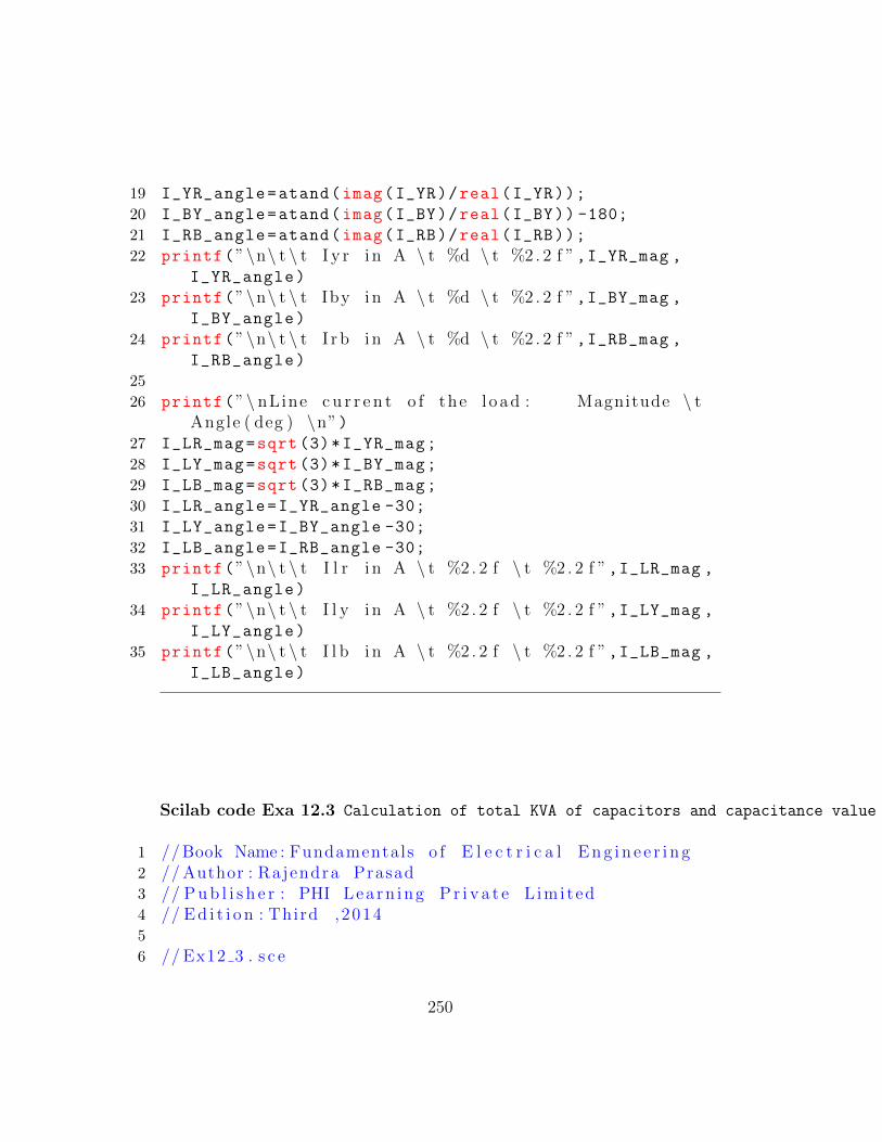
19 I_YR_angle=atand(imag(I_YR)/real(I_YR));
20 I_BY_angle=atand(imag(I_BY)/real(I_BY)) -180;
21 I_RB_angle=atand(imag(I_RB)/real(I_RB));
22 printf(”\n\ t \ t I y r i n A \ t %d \ t %2 . 2 f ”,I_YR_mag ,I_YR_angle)
23 printf(”\n\ t \ t Iby i n A \ t %d \ t %2 . 2 f ”,I_BY_mag ,I_BY_angle)
24 printf(”\n\ t \ t I r b i n A \ t %d \ t %2 . 2 f ”,I_RB_mag ,I_RB_angle)
25
26 printf(”\ nLine c u r r e n t o f the l oad : Magnitude \ tAngle ( deg ) \n”)
27 I_LR_mag=sqrt (3)*I_YR_mag;
28 I_LY_mag=sqrt (3)*I_BY_mag;
29 I_LB_mag=sqrt (3)*I_RB_mag;
30 I_LR_angle=I_YR_angle -30;
31 I_LY_angle=I_BY_angle -30;
32 I_LB_angle=I_RB_angle -30;
33 printf(”\n\ t \ t I l r i n A \ t %2 . 2 f \ t %2 . 2 f ”,I_LR_mag ,I_LR_angle)
34 printf(”\n\ t \ t I l y i n A \ t %2 . 2 f \ t %2 . 2 f ”,I_LY_mag ,I_LY_angle)
35 printf(”\n\ t \ t I l b i n A \ t %2 . 2 f \ t %2 . 2 f ”,I_LB_mag ,I_LB_angle)
Scilab code Exa 12.3 Calculation of total KVA of capacitors and capacitance value
1 // Book Name : Fundamentals o f E l e c t r i c a l E n g i n e e r i n g2 // Author : Rajendra Prasad3 // P u b l i s h e r : PHI Lea rn ing P r i v a t e L imi ted4 // E d i t i o n : Third ,20145
6 // Ex12 3 . s c e
250

Figure 12.3: Calculation of total KVA of capacitors and capacitance value
7
8 clc;
9 clear;
10 P=36; // power i n k i l o w a t t11 Vl=440;
12 f=50;
13 efficiency =0.89;
14 pf1 =0.85;
15 pf2 =0.95;
16 P_not=P/3;
17 P_input=P_not/efficiency;
18 Q1=P_input*tand(acosd(pf1));
19 Q2=P_input*tand(acosd(pf2));
20 Qc=Q1-Q2;
21 kVA =3*Qc;
22 printf(”\n Tota l kVA o f the c a p a c i t o r s f o r r a i s i n gpower f a c t o r to 0 . 9 5 i s %2 . 2 f kVAR \n”,kVA)
23 V=Vl/sqrt (3);
24 Xc=V^2/(Qc*1e3);
25
26 printf(”\n ( a ) ”)27 C_star =1/(2* %pi*f*Xc);
251

Figure 12.4: Calculation of total KVA of capacitors and capacitance value
28 printf(”\n Requ i red c a p a c i t a n c e per phase f o r s t a rconnec t ed c a p a c i t o r s=%3 . 3 f micro−f a r a d \n”,C_star/1e-6)
29
30 printf(”\n ( b ) ”)31 C_delta=C_star /3;
32 printf(”\n Requ i red c a p a c i t a n c e per phase f o r d e l t aconnec t ed c a p a c i t o r s=%2 . 2 f micro−f a r a d \n”,C_delta /1e-6)
33 // Answer vary dueto round o f f e r r o r
Scilab code Exa 12.4 Calculation of total KVA of capacitors and capacitance value
1 // Book Name : Fundamentals o f E l e c t r i c a l E n g i n e e r i n g2 // Author : Rajendra Prasad3 // P u b l i s h e r : PHI Lea rn ing P r i v a t e L imi ted
252

4 // E d i t i o n : Third ,20145
6 // Ex12 4 . s c e7
8
9 //The input data taken from Example : 1 2 . 310 clc;
11 clear;
12 P=36;
13 Vl=440;
14 f=50;
15 efficiency =0.89;
16 pf1 =0.85;
17 pf2 =0.95;
18 Pm=P/efficiency;
19 Qm=Pm*tand(acosd(pf1));
20 Qs=Pm*tand(acosd(pf2));
21 Qc=Qm-Qs;
22 Qc_phase=Qc/3;
23 kVA=Qc_phase;
24 printf(”\n Tota l kVA o f the c a p a c i t o r s f o r r a i s i n gpower f a c t o r to 0 . 9 5 i s %2 . 2 f kVAR \n”,Qc)
25
26 printf(”\n ( a ) ”)27 Vph=Vl/sqrt (3);
28 Iph=kVA*1e3/Vph;
29 C=Iph /(2* %pi*f*Vph);
30 printf(”\n Requ i red c a p a c i t a n c e per phase f o r s t a rconnec t ed c a p a c i t o r s=%3 . 3 f micro−f a r a d \n”,C/1e-6)
31
32 printf(”\n ( b ) ”)33 Vph=Vl;
34 Iph=kVA*1e3/Vph;
35 C=Iph /(2* %pi*f*Vph);
36 printf(”\n Requ i red c a p a c i t a n c e per phase f o r d e l t aconnec t ed c a p a c i t o r s=%3 . 3 f micro−f a r a d \n”,C/1e-6)
253

Figure 12.5: Calculation of line current and neutral current
37 // Answer vary dueto round o f f e r r o r
Scilab code Exa 12.5 Calculation of line current and neutral current
1 // Book Name : Fundamentals o f E l e c t r i c a l E n g i n e e r i n g2 // Author : Rajendra Prasad3 // P u b l i s h e r : PHI Lea rn ing P r i v a t e L imi ted4 // E d i t i o n : Third ,20145
6 // Ex12 5 . s c e7
8 clc;
9 clear;
10 Vl=440;
254

11 z_mag =40;
12 z_angle =-30;
13 z=complex(z_mag*cosd(z_angle),z_mag*sind(z_angle));
14 Iph=Vl/z;
15 Iph_mag=sqrt(real(Iph)^2+ imag(Iph)^2);
16 Iph_angle=atand(imag(Iph)/real(Iph));
17
18 printf(”\ nLine c u r r e n t o f l o ad : \ t Magnitude \ tAngle ( deg ) \n”)
19 I_R_mag=Iph_mag;
20 I_Y_mag=Iph_mag;
21 I_B_mag=Iph_mag;
22 I_R_angle=Iph_angle -0;
23 I_Y_angle=Iph_angle -120;
24 I_B_angle=Iph_angle +120;
25 printf(”\n\ t \ t I r i n A \t%d \ t %2 . 2 f ”,I_R_mag ,I_R_angle)
26 printf(”\n\ t \ t Iy i n A \t%d \ t %2 . 2 f ”,I_Y_mag ,I_Y_angle)
27 printf(”\n\ t \ t Ib i n A \t%d \ t %2 . 2 f ”,I_B_mag ,I_B_angle)
28
29 I_R=complex(I_R_mag*cosd(I_R_angle),I_R_mag*sind(
I_R_angle))
30 I_Y=complex(I_Y_mag*cosd(I_Y_angle),I_Y_mag*sind(
I_Y_angle))
31 I_B=complex(I_B_mag*cosd(I_B_angle),I_B_mag*sind(
I_B_angle))
32 I_N=I_R+I_Y+I_B;
33 printf(”\n The n e u t r a l c u r r e n t i s %d A”,I_N)
Scilab code Exa 12.6 Determination of complex power and line current
255
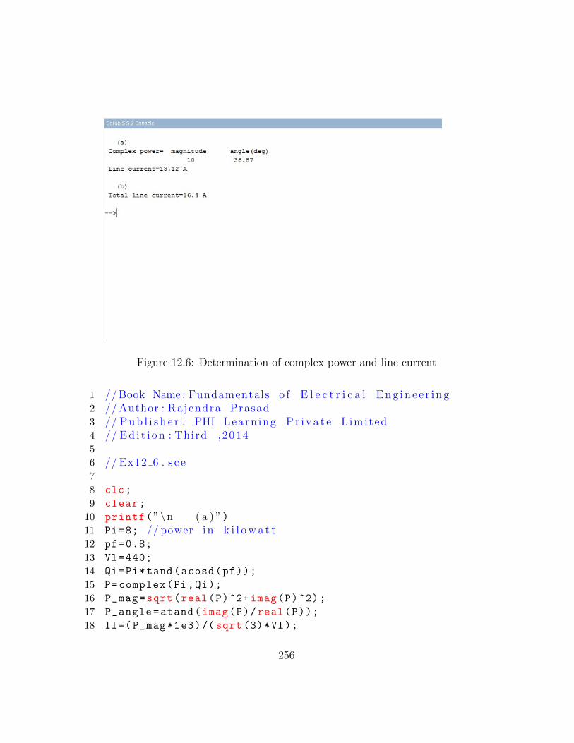
Figure 12.6: Determination of complex power and line current
1 // Book Name : Fundamentals o f E l e c t r i c a l E n g i n e e r i n g2 // Author : Rajendra Prasad3 // P u b l i s h e r : PHI Lea rn ing P r i v a t e L imi ted4 // E d i t i o n : Third ,20145
6 // Ex12 6 . s c e7
8 clc;
9 clear;
10 printf(”\n ( a ) ”)11 Pi=8; // power i n k i l o w a t t12 pf=0.8;
13 Vl=440;
14 Qi=Pi*tand(acosd(pf));
15 P=complex(Pi ,Qi);
16 P_mag=sqrt(real(P)^2+ imag(P)^2);
17 P_angle=atand(imag(P)/real(P));
18 Il=( P_mag*1e3)/(sqrt (3)*Vl);
256

19 printf(”\n Complex power= magnitude \ t a n g l e ( deg ) \n\t \ t %1 . 0 f \ t %2 . 2 f ”,P_mag ,P_angle)
20 printf(”\n Line c u r r e n t=%2 . 2 f A \n”,Il)21
22 printf(”\n ( b ) ”)23 Pl=7.5;
24 pf=0.6;
25 P=Pi+(Pl*pf);
26 Q=Qi -(P*sind(acosd(pf)));
27 kVA=P;
28 Il=(kVA*1e3)/(sqrt (3)*Vl);
29 printf(”\n Tota l l i n e c u r r e n t=%2 . 1 f A \n”,Il)
Scilab code Exa 12.7 Calculation of line current and phase current and total power dissipated
1 // Book Name : Fundamentals o f E l e c t r i c a l E n g i n e e r i n g2 // Author : Rajendra Prasad3 // P u b l i s h e r : PHI Lea rn ing P r i v a t e L imi ted4 // E d i t i o n : Third ,20145
6 // Ex12 7 . s c e7
8 clc;
9 clear;
10 z1=complex (8,6);
11 z2=complex (6,8);
12 z3=complex (4,-3);
13 R_YR=z1;
14 R_BY=z2;
15 R_RB=z3;
16 Vl=440;
17
18 printf(”\n ( a ) De l ta connec t ed l oad o f phase s equence
257
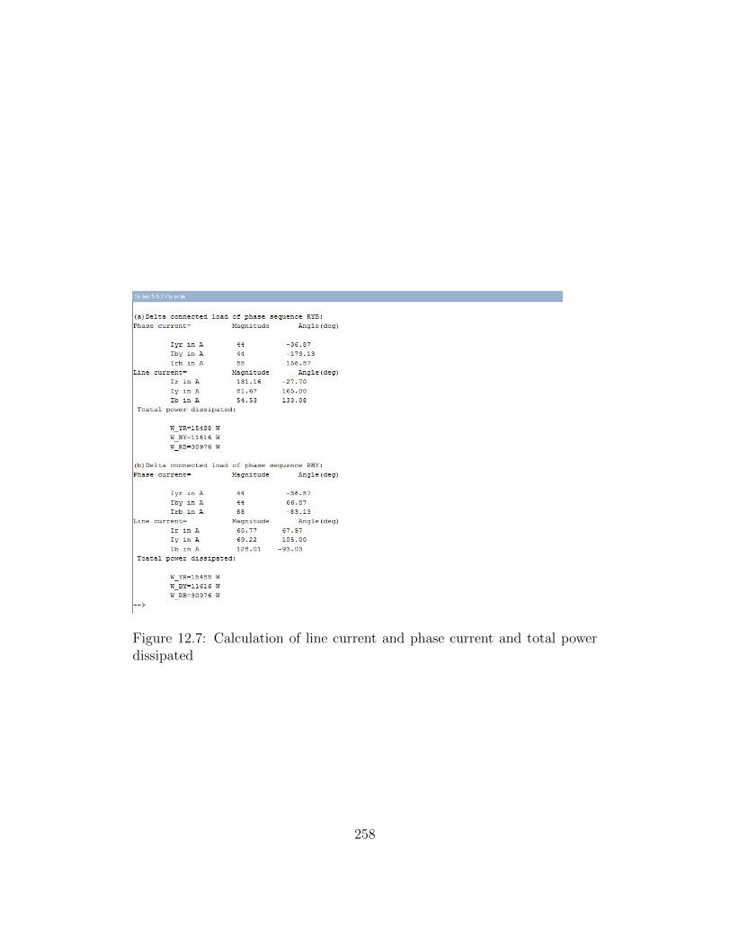
Figure 12.7: Calculation of line current and phase current and total powerdissipated
258
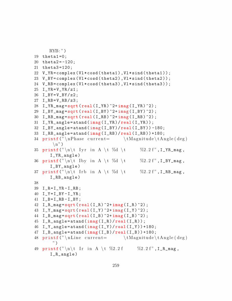
RYB: ”)19 theta1 =0;
20 theta2 = -120;
21 theta3 =120;
22 V_YR=complex(Vl*cosd(theta1),Vl*sind(theta1));
23 V_BY=complex(Vl*cosd(theta2),Vl*sind(theta2));
24 V_RB=complex(Vl*cosd(theta3),Vl*sind(theta3));
25 I_YR=V_YR/z1;
26 I_BY=V_BY/z2;
27 I_RB=V_RB/z3;
28 I_YR_mag=sqrt(real(I_YR)^2+ imag(I_YR)^2);
29 I_BY_mag=sqrt(real(I_BY)^2+ imag(I_BY)^2);
30 I_RB_mag=sqrt(real(I_RB)^2+ imag(I_RB)^2);
31 I_YR_angle=atand(imag(I_YR)/real(I_YR));
32 I_BY_angle=atand(imag(I_BY)/real(I_BY)) -180;
33 I_RB_angle=atand(imag(I_RB)/real(I_RB))+180;
34 printf(”\nPhase c u r r e n t= \ tMagnitude \ tAng le ( deg )\n”)
35 printf(”\n\ t I y r i n A \ t %d \ t %2 . 2 f ”,I_YR_mag ,I_YR_angle)
36 printf(”\n\ t Iby i n A \ t %d \ t %2 . 2 f ”,I_BY_mag ,I_BY_angle)
37 printf(”\n\ t I r b i n A \ t %d \ t %2 . 2 f ”,I_RB_mag ,I_RB_angle)
38
39 I_R=I_YR -I_RB;
40 I_Y=I_BY -I_YR;
41 I_B=I_RB -I_BY;
42 I_R_mag=sqrt(real(I_R)^2+ imag(I_R)^2);
43 I_Y_mag=sqrt(real(I_Y)^2+ imag(I_Y)^2);
44 I_B_mag=sqrt(real(I_B)^2+ imag(I_B)^2);
45 I_R_angle=atand(imag(I_R)/real(I_R));
46 I_Y_angle=atand(imag(I_Y)/real(I_Y))+180;
47 I_B_angle=atand(imag(I_B)/real(I_B))+180;
48 printf(”\ nLine c u r r e n t= \ tMagnitude \ tAng le ( deg )”)
49 printf(”\n\ t I r i n A \ t %2 . 2 f %2 . 2 f ”,I_R_mag ,I_R_angle)
259

50 printf(”\n\ t Iy i n A \ t %2 . 2 f \ t %2 . 2 f ”,I_Y_mag ,I_Y_angle)
51 printf(”\n\ t Ib i n A \ t %2 . 2 f \ t %2 . 2 f ”,I_B_mag ,I_B_angle)
52
53 W_YR=( I_YR_mag)^2* real(z1);
54 W_BY=( I_BY_mag)^2* real(z2);
55 W_RB=( I_RB_mag)^2* real(z3);
56 printf(”\n Toata l power d i s s i p a t e d : \ n”)57 printf(”\n\ t W YR=%d W”,W_YR)58 printf(”\n\ t W BY=%d W”,W_BY)59 printf(”\n\ t W RB=%d W”,W_RB)60
61
62 printf(”\n\n ( b ) De l ta connec t ed l oad o f phases equence RBY: ”)
63 theta1 =0;
64 theta2 =120;
65 theta3 = -120;
66 V_YR=complex(Vl*cosd(theta1),Vl*sind(theta1));
67 V_BY=complex(Vl*cosd(theta2),Vl*sind(theta2));
68 V_RB=complex(Vl*cosd(theta3),Vl*sind(theta3));
69 I_YR=V_YR/z1;
70 I_BY=V_BY/z2;
71 I_RB=V_RB/z3;
72 I_YR_mag=sqrt(real(I_YR)^2+ imag(I_YR)^2);
73 I_BY_mag=sqrt(real(I_BY)^2+ imag(I_BY)^2);
74 I_RB_mag=sqrt(real(I_RB)^2+ imag(I_RB)^2);
75 I_YR_angle=atand(imag(I_YR)/real(I_YR));
76 I_BY_angle=atand(imag(I_BY)/real(I_BY));
77 I_RB_angle=atand(imag(I_RB)/real(I_RB));
78 printf(”\nPhase c u r r e n t= \ tMagnitude \ tAng le ( deg )\n”)
79 printf(”\n\ t I y r i n A \ t %d \ t %2 . 2 f ”,I_YR_mag ,I_YR_angle)
80 printf(”\n\ t Iby i n A \ t %d \ t %2 . 2 f ”,I_BY_mag ,I_BY_angle)
81 printf(”\n\ t I r b i n A \ t %d \ t %2 . 2 f ”,I_RB_mag ,
260

I_RB_angle)
82
83 I_R=I_YR -I_RB;
84 I_Y=I_BY -I_YR;
85 I_B=I_RB -I_BY;
86 I_R_mag=sqrt(real(I_R)^2+ imag(I_R)^2);
87 I_Y_mag=sqrt(real(I_Y)^2+ imag(I_Y)^2);
88 I_B_mag=sqrt(real(I_B)^2+ imag(I_B)^2);
89 I_R_angle=atand(imag(I_R)/real(I_R));
90 I_Y_angle=atand(imag(I_Y)/real(I_Y))+180;
91 I_B_angle=atand(imag(I_B)/real(I_B)) -180;
92 printf(”\ nLine c u r r e n t= \ tMagnitude \ tAng le ( deg )”)
93 printf(”\n\ t I r i n A \ t %2 . 2 f %2 . 2 f ”,I_R_mag ,I_R_angle)
94 printf(”\n\ t Iy i n A \ t %2 . 2 f \ t %2 . 2 f ”,I_Y_mag ,I_Y_angle)
95 printf(”\n\ t Ib i n A \ t %2 . 2 f %2 . 2 f ”,I_B_mag ,I_B_angle)
96
97 W_YR=( I_YR_mag)^2* real(z1);
98 W_BY=( I_BY_mag)^2* real(z2);
99 W_RB=( I_RB_mag)^2* real(z3);
100 printf(”\n Toata l power d i s s i p a t e d : \ n”)101 printf(”\n\ t W YR=%d W”,W_YR)102 printf(”\n\ t W BY=%d W”,W_BY)103 printf(”\n\ t W RB=%d W”,W_RB)
Scilab code Exa 12.8 Calculation of total power and reactive power
1 // Book Name : Fundamentals o f E l e c t r i c a l E n g i n e e r i n g2 // Author : Rajendra Prasad3 // P u b l i s h e r : PHI Lea rn ing P r i v a t e L imi ted
261

Figure 12.8: Calculation of total power and reactive power
262

4 // E d i t i o n : Third ,20145
6 // Ex12 8 . s c e7
8 clc;
9 clear;
10 Vl=110;
11 f=50;
12
13 printf(”\n ( a ) ”)14 R_YR =0;
15 R_BY =100;
16 R_RB =200;
17 W_YR =0; // s i n c e R YR v a l u e i s z e r o18 W_BY=Vl^2/ R_BY;
19 W_RB=Vl^2/ R_RB;
20 printf(”\n Phase power=%3 . 1 f W \n”,W_YR+W_BY+W_RB)21
22
23 printf(”\n ( b ) ”)24 X_YR =95;
25 X_BY =0;
26 X_RB =0;
27 W_YR=Vl^2/ X_YR;
28 W_BY =0; // s i n c e X BY v a l u e i s z e r o29 W_RB =0; // s i n c e X RB v a l u e i s z e r o30 printf(”\n R e a c t i v e power=%3 . 2 f VAR”,W_YR+W_BY+
W_RB)
Scilab code Exa 12.9 Calculation of neutral current and power taken by each phase
1 // Book Name : Fundamentals o f E l e c t r i c a l E n g i n e e r i n g2 // Author : Rajendra Prasad
263

Figure 12.9: Calculation of neutral current and power taken by each phase
3 // P u b l i s h e r : PHI Lea rn ing P r i v a t e L imi ted4 // E d i t i o n : Third ,20145
6 // Ex12 9 . s c e7
8 clc;
9 clear;
10 z=10;
11 ang1 =0;
12 ang2 =37;
13 ang3 =-53;
14 Zr=complex(z*cosd(ang1),z*sind(ang1));
15 Zy=complex(z*cosd(ang2),z*sind(ang2));
16 Zb=complex(z*cosd(ang3),z*sind(ang3));
17
18 printf(”\n ( a ) For phase s equence RYB: \ n”)19 V=220;
20 theta1 =0;
264

21 theta2 = -120;
22 theta3 =120;
23 Vr=complex(V*cosd(theta1),V*sind(theta1));
24 Vy=complex(V*cosd(theta2),V*sind(theta2));
25 Vb=complex(V*cosd(theta3),V*sind(theta3));
26
27 Ir=Vr/Zr;
28 Iy=Vy/Zy;
29 Ib=Vb/Zb;
30 In=Ir+Iy+Ib;
31 In_mag=sqrt(real(In)^2+ imag(In)^2);
32 In_angle=atand(imag(In)/real(In));
33 printf(”\n The c u r r e n t through the n e u t r a l wire , \ n−In=\tMagnitude \ tAng le ( deg ) \n\ t %2 . 2 f \ t %2 . 2 f\n”,In_mag ,In_angle)
34
35 Ir_mag=sqrt(real(Ir)^2+ imag(Ir)^2);
36 Iy_mag=sqrt(real(Iy)^2+ imag(Iy)^2);
37 Ib_mag=sqrt(real(Ib)^2+ imag(Ib)^2);
38 Pr=( Ir_mag)^2* real(Zr);
39 Py=( Iy_mag)^2* real(Zy);
40 Pb=( Ib_mag)^2* real(Zb);
41 printf(”\n Power taken by each l oad : \ n\ t Pr=%d W \n\ t Py=%4 . 1 f W \n\ t Pb=%4 . 1 f W \n”, Pr, Py, Pb)
42
43
44
45 printf(”\n\n ( b ) For phase s equence RBY: \ n”)46 V=220;
47 theta1 =0;
48 theta2 =120;
49 theta3 = -120;
50 Vr=complex(V*cosd(theta1),V*sind(theta1));
51 Vy=complex(V*cosd(theta2),V*sind(theta2));
52 Vb=complex(V*cosd(theta3),V*sind(theta3));
53
54 Ir=Vr/Zr;
55 Iy=Vy/Zy;
265

56 Ib=Vb/Zb;
57 In=Ir+Iy+Ib;
58 In_mag=sqrt(real(In)^2+ imag(In)^2);
59 In_angle=atand(imag(In)/real(In));
60 printf(”\n The c u r r e n t through the n e u t r a l wire , \ nIn=\tMagnitude \ tAng le ( deg ) \n\ t %2 . 2 f \ t %2 . 2 f\n”,In_mag ,In_angle)
61
62 Ir_mag=sqrt(real(Ir)^2+ imag(Ir)^2);
63 Iy_mag=sqrt(real(Iy)^2+ imag(Iy)^2);
64 Ib_mag=sqrt(real(Ib)^2+ imag(Ib)^2);
65 Pr=( Ir_mag)^2* real(Zr);
66 Py=( Iy_mag)^2* real(Zy);
67 Pb=( Ib_mag)^2* real(Zb);
68 printf(”\n Power taken by each l oad : \ n\ t Pr=%d W \n\ t Py=%4 . 1 f W \n\ t Pb=%4 . 1 f W \n”, Pr, Py, Pb)
Scilab code Exa 12.10 Determination of phase voltage and current
1 // Book Name : Fundamentals o f E l e c t r i c a l E n g i n e e r i n g2 // Author : Rajendra Prasad3 // P u b l i s h e r : PHI Lea rn ing P r i v a t e L imi ted4 // E d i t i o n : Third ,20145
6 // Ex12 10 . s c e7
8 clc;
9 clear;
10 Z_R=complex (8,6);
11 Z_Y=complex (8,-6);
12 Z_B=complex (5,0);
13 Z_N=complex (0.5 ,1);
14 Y_R =1/Z_R;
266

Figure 12.10: Determination of phase voltage and current
15 Y_Y =1/Z_Y;
16 Y_B =1/Z_B;
17 Y_N =1/Z_N;
18 E_R =220;
19 E_Y =220;
20 E_B =220;
21 theta1 =0;
22 theta2 = -120;
23 theta3 =120;
24 V_R=complex(E_R*cosd(theta1),E_R*sind(theta1));
25 V_Y=complex(E_Y*cosd(theta2),E_Y*sind(theta2));
26 V_B=complex(E_B*cosd(theta3),E_B*sind(theta3));
27 V_NN_dash =((V_R*Y_R)+(V_Y*Y_Y)+(V_B*Y_B))/(Y_R+Y_Y+
Y_B+Y_N);
28
29 V_R_dash=V_R -V_NN_dash;
30 V_Y_dash=V_Y -V_NN_dash;
31 V_B_dash=V_B -V_NN_dash;
267

32 V_R_dash_mag=sqrt(real(V_R_dash)^2+ imag(V_R_dash)^2)
;
33 V_Y_dash_mag=sqrt(real(V_Y_dash)^2+ imag(V_Y_dash)^2)
;
34 V_B_dash_mag=sqrt(real(V_B_dash)^2+ imag(V_B_dash)^2)
;
35 V_R_dash_angle=atand(imag(V_R_dash)/real(V_R_dash));
36 V_Y_dash_angle=atand(imag(V_Y_dash)/real(V_Y_dash))
+180;
37 V_B_dash_angle=atand(imag(V_B_dash)/real(V_B_dash))
+180;
38 printf(”\n Load phase v o l t a g e s : Magnitude \ tAng le ( deg) ”)
39 printf(”\n For R phase \t%3 . 2 f \t%0 . 3 f ”,V_R_dash_mag ,V_R_dash_angle)
40 printf(”\n For Y phase \t%3 . 2 f \t%3 . 2 f ”,V_Y_dash_mag ,V_Y_dash_angle)
41 printf(”\n For B phase \t%3 . 2 f \t%3 . 2 f ”,V_B_dash_mag ,V_B_dash_angle)
42 // For V NN dash v a l u e , the answer g i v e n i n the booki s wrong . So l oad phase v o l t a g e vary from the
book answer .43 // Also V R dash a n g l e i s not 0 . 1 6 8 . I t i s n e g a t i v e
a n g l e tha t i s −0.19344 I_R=V_R_dash*Y_R;
45 I_Y=V_Y_dash*Y_Y;
46 I_B=V_B_dash*Y_B;
47 I_N=V_NN_dash*Y_N;
48 I_R_mag=sqrt(real(I_R)^2+ imag(I_R)^2);
49 I_Y_mag=sqrt(real(I_Y)^2+ imag(I_Y)^2);
50 I_B_mag=sqrt(real(I_B)^2+ imag(I_B)^2);
51 I_N_mag=sqrt(real(I_N)^2+ imag(I_N)^2);
52 I_R_angle=atand(imag(I_R)/real(I_R));
53 I_Y_angle=atand(imag(I_Y)/real(I_Y))+360;
54 I_B_angle=atand(imag(I_B)/real(I_B))+180;
55 I_N_angle=atand(imag(I_N)/real(I_N))+180;
56 printf(”\n\n Load phase c u r r e n t : Magnitude \ tAng le (deg ) ”)
268

Figure 12.11: Calculation of each branch voltage and current
57 printf(”\n For R phase \t%3 . 2 f \t%0 . 3 f ”,I_R_mag ,I_R_angle)
58 printf(”\n For Y phase \t%3 . 2 f \t%3 . 2 f ”,I_Y_mag ,I_Y_angle)
59 printf(”\n For B phase \t%3 . 2 f \t%3 . 2 f ”,I_B_mag ,I_B_angle)
60 printf(”\n For Neut ra l \t%3 . 2 f \t%3 . 2 f ”,I_N_mag ,I_N_angle)
Scilab code Exa 12.11 Calculation of each branch voltage and current
1 // Book Name : Fundamentals o f E l e c t r i c a l E n g i n e e r i n g2 // Author : Rajendra Prasad3 // P u b l i s h e r : PHI Lea rn ing P r i v a t e L imi ted
269

4 // E d i t i o n : Third ,20145
6 // Ex12 11 . s c e7
8 clc;
9 clear;
10 Vl=400;
11 V=Vl/sqrt (3);
12 Z_R=complex (20* cosd (30) ,20*sind (30));
13 Z_Y=complex (40* cosd (60) ,40*sind (60));
14 Z_B=complex (10* cosd (-90) ,10*sind (-90));
15 Y_R =1/Z_R;
16 Y_Y =1/Z_Y;
17 Y_B =1/Z_B;
18 theta1 =0;
19 theta2 = -120;
20 theta3 =120;
21 V_R=complex(V*cosd(theta1),V*sind(theta1));
22 V_Y=complex(V*cosd(theta2),V*sind(theta2));
23 V_B=complex(V*cosd(theta3),V*sind(theta3));
24 V_NN_dash =((V_R*Y_R)+(V_Y*Y_Y)+(V_B*Y_B))/(Y_R+Y_Y+
Y_B);
25 V_R_dash=V_R -V_NN_dash;
26 V_Y_dash=V_Y -V_NN_dash;
27 V_B_dash=V_B -V_NN_dash;
28 V_R_dash_mag=sqrt(real(V_R_dash)^2+ imag(V_R_dash)^2)
;
29 V_Y_dash_mag=sqrt(real(V_Y_dash)^2+ imag(V_Y_dash)^2)
;
30 V_B_dash_mag=sqrt(real(V_B_dash)^2+ imag(V_B_dash)^2)
;
31 V_R_dash_angle=atand(imag(V_R_dash)/real(V_R_dash));
32 V_Y_dash_angle=atand(imag(V_Y_dash)/real(V_Y_dash));
33 V_B_dash_angle=atand(imag(V_B_dash)/real(V_B_dash));
34 printf(”\n\n Phase v o l t a g e s : Magnitude \ tAng le (deg ) ”)
35 printf(”\n For R phase \t%3 . 2 f \t%0 . 3 f ”,V_R_dash_mag ,V_R_dash_angle)
270

36 printf(”\n For Y phase \t%3 . 2 f \t%3 . 2 f ”,V_Y_dash_mag ,V_Y_dash_angle)
37 printf(”\n For B phase \t%3 . 0 f \t%3 . 2 f ”,V_B_dash_mag ,V_B_dash_angle)
38
39 I_R=V_R_dash*Y_R;
40 I_Y=V_Y_dash*Y_Y;
41 I_B=V_B_dash*Y_B;
42 I_R_mag=sqrt(real(I_R)^2+ imag(I_R)^2);
43 I_Y_mag=sqrt(real(I_Y)^2+ imag(I_Y)^2);
44 I_B_mag=sqrt(real(I_B)^2+ imag(I_B)^2);
45 I_R_angle=atand(imag(I_R)/real(I_R));
46 I_Y_angle=atand(imag(I_Y)/real(I_Y)) -180;
47 I_B_angle=atand(imag(I_B)/real(I_B))+180;
48 printf(”\n Phase c u r r e n t : Magnitude \ tAng le ( deg ) ”)
49 printf(”\n For R phase \t%2 . 2 f \t%0 . 3 f ”,I_R_mag ,I_R_angle)
50 printf(”\n For Y phase \t%1 . 2 f \t%3 . 2 f ”,I_Y_mag ,I_Y_angle)
51 printf(”\n For B phase \t%2 . 0 f \t%3 . 2 f ”,I_B_mag ,I_B_angle)
52
53 // Answer vary due to r o u n d o f f e r r o r
Scilab code Exa 12.12 Calculation of line current or star phase current
1 // Book Name : Fundamentals o f E l e c t r i c a l E n g i n e e r i n g2 // Author : Rajendra Prasad3 // P u b l i s h e r : PHI Lea rn ing P r i v a t e L imi ted4 // E d i t i o n : Third ,20145
6 // Ex12 12 . s c e
271
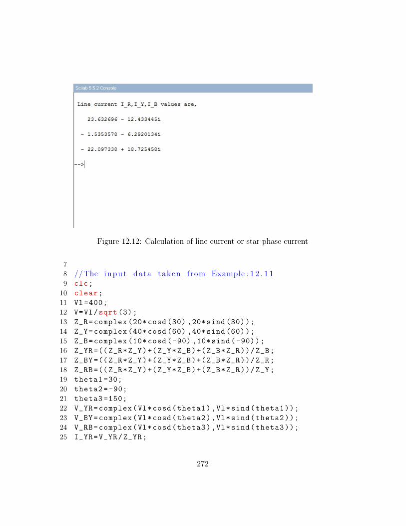
Figure 12.12: Calculation of line current or star phase current
7
8 //The input data taken from Example : 1 2 . 1 19 clc;
10 clear;
11 Vl=400;
12 V=Vl/sqrt (3);
13 Z_R=complex (20* cosd (30) ,20*sind (30));
14 Z_Y=complex (40* cosd (60) ,40*sind (60));
15 Z_B=complex (10* cosd (-90) ,10*sind (-90));
16 Z_YR =((Z_R*Z_Y)+(Z_Y*Z_B)+(Z_B*Z_R))/Z_B;
17 Z_BY =((Z_R*Z_Y)+(Z_Y*Z_B)+(Z_B*Z_R))/Z_R;
18 Z_RB =((Z_R*Z_Y)+(Z_Y*Z_B)+(Z_B*Z_R))/Z_Y;
19 theta1 =30;
20 theta2 =-90;
21 theta3 =150;
22 V_YR=complex(Vl*cosd(theta1),Vl*sind(theta1));
23 V_BY=complex(Vl*cosd(theta2),Vl*sind(theta2));
24 V_RB=complex(Vl*cosd(theta3),Vl*sind(theta3));
25 I_YR=V_YR/Z_YR;
272

Figure 12.13: Calculation of line current
26 I_BY=V_BY/Z_BY;
27 I_RB=V_RB/Z_RB;
28 I_R=I_YR -I_RB;
29 I_Y=I_BY -I_YR;
30 I_B=I_RB -I_BY;
31 printf(”\n Line c u r r e n t I R , I Y , I B v a l u e s are , \ n”)32 disp(I_R)
33 disp(I_Y)
34 disp(I_B)
Scilab code Exa 12.13 Calculation of line current
273

1 // Book Name : Fundamentals o f E l e c t r i c a l E n g i n e e r i n g2 // Author : Rajendra Prasad3 // P u b l i s h e r : PHI Lea rn ing P r i v a t e L imi ted4 // E d i t i o n : Third ,20145
6 // Ex12 13 . s c e7
8 //The input data taken from Example : 1 2 . 1 19 clc;
10 clear;
11 Vl=400;
12 V=Vl/sqrt (3);
13 Z_R=complex (20* cosd (30) ,20*sind (30));
14 Z_Y=complex (40* cosd (60) ,40*sind (60));
15 Z_B=complex (10* cosd (-90) ,10*sind (-90));
16 theta1 =30;
17 theta2 =-90;
18 theta3 =150;
19 V_YR=complex(Vl*cosd(theta1),Vl*sind(theta1));
20 V_BY=complex(Vl*cosd(theta2),Vl*sind(theta2));
21 V_RB=complex(Vl*cosd(theta3),Vl*sind(theta3));
22
23 I_R =(( V_YR*Z_B)-(V_RB*Z_Y))/((Z_R*Z_Y)+(Z_Y*Z_B)+(
Z_B*Z_R));
24 I_Y =(( V_BY*Z_R)-(V_YR*Z_B))/((Z_R*Z_Y)+(Z_Y*Z_B)+(
Z_B*Z_R));
25 I_B =(( V_RB*Z_Y)-(V_BY*Z_R))/((Z_R*Z_Y)+(Z_Y*Z_B)+(
Z_B*Z_R));
26 printf(”\n Line c u r r e n t I R , I Y , I B v a l u e s are , \n”)
27 disp(I_R)
28 disp(I_Y)
29 disp(I_B)
274

Chapter 13
Dynamic Response of Network
Scilab code Exa 13.1 Calculation of resistance
1 // Book Name : Fundamentals o f E l e c t r i c a l E n g i n e e r i n g2 // Author : Rajendra Prasad3 // P u b l i s h e r : PHI Lea rn ing P r i v a t e L imi ted4 // E d i t i o n : Third ,20145
6 // Ex13 1 . s c e .7
8 clc;
9 clear;
10 Vc=60;
11 V_not =120;
12 t=20;
13 C=10e-6;
14 R=-t/(C*log(Vc/V_not));
15 printf(”\n The v a l u e o f r e s i s t a n c e=%1 . 3 f mega ohm”,R*1e-6)
275

Figure 13.1: Calculation of resistance
Figure 13.2: Determination of current and time
276
Scilab code Exa 13.2 Determination of current and time
1 // Book Name : Fundamentals o f E l e c t r i c a l E n g i n e e r i n g2 // Author : Rajendra Prasad3 // P u b l i s h e r : PHI Lea rn ing P r i v a t e L imi ted4 // E d i t i o n : Third ,20145
6 // Ex13 2 . s c e7
8 clc;
9 clear;
10 R1=60;
11 R2=80;
12 C=100e-6;
13 V=12;
14 t1=6e-3;
15 i_S =300e-3;
16 i_R=V/R1;
17 i_C=(V/R2)*exp(-t1/(R2*C));
18 i=i_R+i_C;
19 printf(”\n The c u r r e n t drawn from the s o u r c e=%3 . 0 fmA \n”,i*1e3)
20 I_C=i_S -i_R;
21 t2=(R2*C)*log(V/(R2*I_C));
22 printf(”\n Time f o r draw the c u r r e n t o f 300 mA fromthe s o u r c e=%1 . 3 f ms \n”,t2*1e3)
Scilab code Exa 13.5 Determination of time constant and damping ratio and current
1 // Book Name : Fundamentals o f E l e c t r i c a l E n g i n e e r i n g
277

Figure 13.3: Determination of time constant and damping ratio and current
2 // Author : Rajendra Prasad3 // P u b l i s h e r : PHI Lea rn ing P r i v a t e L imi ted4 // E d i t i o n : Third ,20145
6 // Ex13 5 . s c e7
8 clc;
9 clear;
10 V=100;
11 R=2;
12 L=10;
13 t=8;
14 T=L/R;
15 printf(”\n Time c o n s t a n t=%d s e c \n”,T)16 del=R/L;
17 printf(”\n Damping r a t i o=%1 . 1 f \n”,del)18 I=(V/R)*(1-exp(-t/T));
19 printf(”\n The v a l u e o f c u r r e n t o f a f t e r 8 s e c o n d so f s w i t c h i n g=%2 . 1 f A \n”,I)
278

Figure 13.4: Determination of current values
Scilab code Exa 13.6 Determination of current values
1 // Book Name : Fundamentals o f E l e c t r i c a l E n g i n e e r i n g2 // Author : Rajendra Prasad3 // P u b l i s h e r : PHI Lea rn ing P r i v a t e L imi ted4 // E d i t i o n : Third ,20145
6 // Ex13 6 . s c e7
8 clc;
9 clear;
10 R=20;
279

Figure 13.5: Calculation of current ratio
11 L=0.5;
12 V=100;
13 R_S =10;
14 t1=0;
15 t2=50e-3;
16 Req=R+R_S;
17 T1=L/Req;//Time c o n s t a n t 118 T2=L/R;//Time c o n s t a n t 219 I=V/Req;
20 printf(”\n Steady s t a t e c u r r e n t=%1 . 3 f A \n”,I)21 i=I*exp(-t2/T2);
22 printf(”\n The v a l u e o f c u r r e n t a f t e r 50 ms=%0 . 2 f A\n”,i)
280

Scilab code Exa 13.7 Calculation of current ratio
1 // Book Name : Fundamentals o f E l e c t r i c a l E n g i n e e r i n g2 // Author : Rajendra Prasad3 // P u b l i s h e r : PHI Lea rn ing P r i v a t e L imi ted4 // E d i t i o n : Third ,20145
6 // Ex13 7 . s c e7
8 clc;
9 clear;
10 R=10;
11 L=0.1;
12 t1 =0.01;
13 omega =100* %pi;
14 phi=omega*t1;
15 t=(asin (1)+atan(( omega*L)/R))/omega;
16 Imax=((- omega*L*exp(-R*t/L))/(R^2+( omega*L)^2))-(sin
((100* %pi*t) -(atan(omega*L/R)))/sqrt(R^2+( omega*L
)^2));
17 t=0;
18 Iss=((-omega*L*exp(-R*t/L))/(R^2+( omega*L)^2))-(sind
((100* %pi*t) -(atan(omega*L/R)))/sqrt(R^2+( omega*L
)^2));
19 a=Imax/Iss;
20 printf(”\n Rat io o f maximum v a l u e o f c u r r e n t tos t e ady s t a t e v a l u e o f c u r r e n t=%1 . 2 f \n”,a)
21 // Answer vary dueto round o f f e r r o r i n ’ t ’c a l c u l a t i o n
281

Figure 13.6: Determination of current
Scilab code Exa 13.14 Determination of current
1 // Book Name : Fundamentals o f E l e c t r i c a l E n g i n e e r i n g2 // Author : Rajendra Prasad3 // P u b l i s h e r : PHI Lea rn ing P r i v a t e L imi ted4 // E d i t i o n : Third ,20145
6 // Ex13 14 . s c e7
8 clc;
9 clear;
10 //From Ex 13 . 211 Id=300e-3;
12 t=6e-3;
13 V=12;
14 R=60;
15 Ir=V/R;
282

16 Ic1 =0.15* exp(-125*t); // i t Obtain , a f t e r thes i m p l i f i c a t i o n o f l oop e q u a t i o n
17 I=Ir+Ic1;
18 printf(”\n Current drawn from the l oad a f t e r 6 ms=%3. 0 f mA \n”,I*1e3)
19 Ic2=Id -Ir;
20 t=log(Ic2 /0.15) / -125;
21 printf(”\n The t ime when c u r r e n t drawn from thes o u r c e i s 0 . 3 A=%1 . 3 f ms \n”,t*1e3)
283

Chapter 14
Electrical Power System
Scilab code Exa 14.1 Calculation of average load and energy consumption and load factor
1 // Book Name : Fundamentals o f E l e c t r i c a l E n g i n e e r i n g2 // Author : Rajendra Prasad3 // P u b l i s h e r : PHI Lea rn ing P r i v a t e L imi ted4 // E d i t i o n : Third ,20145
6 // Ex14 1 . s c e .7
8 clc;
9 clear;
10 maximum_demand =1.5e3;
11 total_lamps =10;
12 lamps_on =7;
13 lamp_ontime =5;
14 lamp_power =100;
15 heater_on =2;
16 heater_ontime =3;
17 heater_power =1e3;
18 printf(”\n ( a ) ”)19 actual_energy_consumed =( lamps_on*lamp_power*
284

Figure 14.1: Calculation of average load and energy consumption and loadfactor
lamp_ontime)+( heater_on*heater_power*
heater_ontime);
20 time_duration =24;
21 average_load =( actual_energy_consumed)/( time_duration
);
22 printf(”\n Average l oad=%3 . 2 f W \n”,average_load)23
24 printf(”\n ( b ) ”)25 monthly_energy_consump=actual_energy_consumed *30*1e
-3;
26 printf(”\n Monthly ene rgy consumption=%3 . 0 f kW \n”,monthly_energy_consump)
27
28 printf(”\n ( c ) ”)29 load_factor=average_load/maximum_demand;
30 printf(”\n Load f a c t o r=%1 . 3 f \n”,load_factor)
285

Figure 14.2: Determination of diversity factor and load factor and combinedaverage load
Scilab code Exa 14.2 Determination of diversity factor and load factor and combined average load
1 // Book Name : Fundamentals o f E l e c t r i c a l E n g i n e e r i n g2 // Author : Rajendra Prasad3 // P u b l i s h e r : PHI Lea rn ing P r i v a t e L imi ted4 // E d i t i o n : Third ,20145
6 // Ex14 2 . s c e .7
8 clc;
286
9 clear;
10 // Loads a r e i n k i l o w a t t11 avg_load1 =1;
12 avg_load2 =0.3;
13 avg_load3 =0.5;
14 avg_load4 =2.5;
15 max_load1 =5;
16 max_load2 =2;
17 max_load3 =2;
18 max_load4 =10;
19 max_demand1 =5;
20 max_demand2 =1.6;
21 max_demand3 =1;
22 max_demand4 =5;
23
24 printf(”\n ( a ) ”)25 sumof_individualmax_dem=max_load1+max_load2+
max_load3+max_load4;
26 max_demandof_wholegroup=max_demand1+max_demand2+
max_demand3+max_demand4;
27 diversity_factor=sumof_individualmax_dem/
max_demandof_wholegroup;
28 printf(”\n D i v e r s i t y f a c t o r=%1 . 4 f \n”,diversity_factor)
29
30
31 printf(”\n ( b ) ”)32 LF_of_consumer1=avg_load1/max_load1;
33 printf(”\n Load f a c t o r o f consumer1 =%1 . 2 f \n”,LF_of_consumer1)
34 LF_of_consumer2=avg_load2/max_load2;
35 printf(”\n Load f a c t o r o f consumer2 =%1 . 2 f \n”,LF_of_consumer2)
36 LF_of_consumer3=avg_load3/max_load3;
37 printf(”\n Load f a c t o r o f consumer3 =%1 . 2 f \n”,LF_of_consumer3)
38 LF_of_consumer4=avg_load4/max_load4;
39 printf(”\n Load f a c t o r o f consumer4 =%1 . 2 f \n”,
287

Figure 14.3: Calculation of annual bill of the consumer
LF_of_consumer4)
40
41 printf(”\n ( c ) ”)42 combined_avg_load =( avg_load1+avg_load2+avg_load3+
avg_load4);
43 printf(”\n Combined ave rage l oad =%1 . 1 f kW \n”,combined_avg_load)
44 combined_load_factor=combined_avg_load/
max_demandof_wholegroup;
45 printf(”\n Combined l oad f a c t o r =%1 . 3 f \n”,combined_load_factor)
Scilab code Exa 14.3 Calculation of annual bill of the consumer
288
1 // Book Name : Fundamentals o f E l e c t r i c a l E n g i n e e r i n g2 // Author : Rajendra Prasad3 // P u b l i s h e r : PHI Lea rn ing P r i v a t e L imi ted4 // E d i t i o n : Third ,20145
6 // Ex14 3 . s c e .7
8 clc;
9 clear;
10 average_demand =33.75; // i nk i l o w a t t
11 time_duration =24*365; // i n hours12 tariff =1.25; // i n r u p e e s
per k i l o w a t t h o u r13 annualenergy_consumption=average_demand*
time_duration;
14 C=annualenergy_consumption*tariff;
15 printf(” \n Annual b i l l o f the consumer=%6 . 1 f r u p e e s\n”,C)
Scilab code Exa 14.4 Calculation of overall cost per kWh
1 // Book Name : Fundamentals o f E l e c t r i c a l E n g i n e e r i n g2 // Author : Rajendra Prasad3 // P u b l i s h e r : PHI Lea rn ing P r i v a t e L imi ted4 // E d i t i o n : Third ,20145
6 // Ex14 4 . s c e .7
8 clc;
9 clear;
10 max_demand =75; // i n k i l o w a t t11 time_duration =24*365; // i n hour
289

Figure 14.4: Calculation of overall cost per kWh
12 load_factor =0.45;
13 tariff1 =650;
14 tariff2 =1.30;
15 annual_energy_consump=max_demand*time_duration*
load_factor;
16 Ce=tariff2*annual_energy_consump;
17 Cf=tariff1*max_demand;
18 total_annualcharge=Ce+Cf;
19 overall_costperkwhr=total_annualcharge/
annual_energy_consump;
20 printf(” \n O v e r a l l c o s t per kWh= %1. 2 f r u p e e s \n”,overall_costperkwhr)
Scilab code Exa 14.5 Calculation of monthly bill of the consumer
290
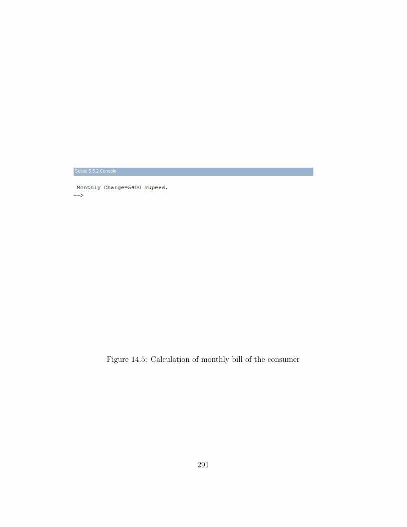
Figure 14.5: Calculation of monthly bill of the consumer
291

1 // Book Name : Fundamentals o f E l e c t r i c a l E n g i n e e r i n g2 // Author : Rajendra Prasad3 // P u b l i s h e r : PHI Lea rn ing P r i v a t e L imi ted4 // E d i t i o n : Third ,20145
6 // Ex14 5 . s c e7
8 clc;
9 clear;
10 tariff1 =3.50; // t a r i f f i n r u p e e s perk i l o w a t t h o u r f o r f i r s t 500 k i l o w a t t h o u r
11 tariff2 =3.00; // t a r i f f i n r u p e e s perk i l o w a t t h o u r f o r next 500 k i l o w a t t h o u r
12 tariff3 =2.50; // t a r i f f i n r u p e e s perk i l o w a t t h o u r f o r usage e x c e e d i n g 1000 k i l o w a t t h o u r
13 days_in_a_month =31;
14 time_duration =24* days_in_a_month;
15 average_demand =2.5; //i n k i l o w a t t
16 monthly_consumption=time_duration*average_demand;
17 a1=500; //kWh f o r t a r i f f 118 a2=500; //kWh f o r t a r i f f 219 a3=monthly_consumption -a1-a2; //kWh f o r
t a r i f f 320 monthly_charge =(a1*tariff1)+(a2*tariff2)+(a3*tariff3
);
21 printf(”\n Monthly Charge=%d r u p e e s . ”,monthly_charge)
Scilab code Exa 14.6 Calculation of annual bill of the consumer
1 // Book Name : Fundamentals o f E l e c t r i c a l E n g i n e e r i n g2 // Author : Rajendra Prasad
292

Figure 14.6: Calculation of annual bill of the consumer
3 // P u b l i s h e r : PHI Lea rn ing P r i v a t e L imi ted4 // E d i t i o n : Third ,20145
6 // Ex14 6 . s c e .7
8 clc;
9 clear;
10 average_demand =450;
11 load_factor =0.65;
12 power_factor =0.8;
13 tariff1 =75; // i n r u e e s per month per kVA14 tariff2 =1.30; // i n r u p e e s per k i l o w a t t h o u r15 working_time =8*300;
16 maximum_kw_demand=average_demand/load_factor;
17 maximum_kVA_demand=maximum_kw_demand/power_factor;
18 annual_energy_charge=tariff2*average_demand*
working_time;
19 annual_max_demand_charge=tariff1 *12*
293

maximum_kVA_demand;
20 annual_charge=annual_energy_charge+
annual_max_demand_charge;
21 disp(annual_charge , ’ Annual b i l l o f the consumer i nr u p e e s ’ )
22 //The answer vary dueto r o u n d o f f e r r o r .
294

Chapter 15
Domestic Lighting
Scilab code Exa 15.1 Calculation of lamp efficiency and luminous intensity and MSCP
1 // Book Name : Fundamentals o f E l e c t r i c a l E n g i n e e r i n g2 // Author : Rajendra Prasad3 // P u b l i s h e r : PHI Lea rn ing P r i v a t e L imi ted4 // E d i t i o n : Third ,20145
6 // Ex15 1 . s c e7
8 clc;
9 clear;
10 W=100;
11 V=250;
12 light_flux =3000;
13 printf(”\n ( a ) ”)14 mew=light_flux/W;
15 printf(”\n Lamp e f f i c i e n c y=%d Lumens/ watt \n”,mew)16
17 printf(”\n ( b ) ”)18 total_solid_angle =(4* %pi);
19 I=light_flux/total_solid_angle;
295

Figure 15.1: Calculation of lamp efficiency and luminous intensity and MSCP
20 printf(”\n Luminous i n t e n s i t y=%3 . 2 f cd \n”,I)21
22 printf(”\n ( c ) ”)23 M.S.C.P=I/W;
24 printf(”\n Mean S p h e r i c a l Candle Power per watt=%1 . 4f cd / watt \n”,M.S.C.P)
Scilab code Exa 15.2 Calculation of average luminance of the sphere
1 // Book Name : Fundamentals o f E l e c t r i c a l E n g i n e e r i n g2 // Author : Rajendra Prasad3 // P u b l i s h e r : PHI Lea rn ing P r i v a t e L imi ted4 // E d i t i o n : Third ,20145
6 // Ex15 2 . s c e
296

Figure 15.2: Calculation of average luminance of the sphere
7
8 clc;
9 clear;
10 d=40e-2;
11 light_flux =5000;
12 absorption_factor =0.2;
13 transmission_factor =0.8;
14 F=light_flux*transmission_factor;
15 A=%pi*d^2;
16 L=F/A;
17 printf(”\n Average luminance o f the s p h e r e=%4 . 1 flumens /mˆ2 \n”,L)
18 // Answer vary due to r o u n d o f f e r r o r i n s u r f a c e a r ea(A) c a l c u l a t i o n
297

Figure 15.3: Determination of illumination
Scilab code Exa 15.3 Determination of illumination
1 // Book Name : Fundamentals o f E l e c t r i c a l E n g i n e e r i n g2 // Author : Rajendra Prasad3 // P u b l i s h e r : PHI Lea rn ing P r i v a t e L imi ted4 // E d i t i o n : Third ,20145
6 // Ex15 3 . s c e7
8 clc;
9 clear;
10 M.S.C.P=1000;
11 h=2.8;
12 x=2.5;
298

Figure 15.4: Calculation of distance between two lamps
13 E=(M.S.C.P*h)/(h^2+x^2) ^(3/2);
14 printf(”\n I l l u m i n a t i o n=%2 . 2 f lux \n”,E)
Scilab code Exa 15.4 Calculation of distance between two lamps
1 // Book Name : Fundamentals o f E l e c t r i c a l E n g i n e e r i n g2 // Author : Rajendra Prasad3 // P u b l i s h e r : PHI Lea rn ing P r i v a t e L imi ted4 // E d i t i o n : Third ,20145
299

6 // Ex15 4 . s c e .7
8 clc;
9 clear;
10 // There i s a mi s take i n the q u e s t i o n , g i v e n h e i g h ti s 5 i n s t e a d o f 4
11 h=4;
12 x=[2:2:14];
13 for i=1: length(x)
14
15 Ed(i)=(64/(4^2+x(i)^2) ^(3/2))+1;
16 Eb(i)=(256/(4^2+(x(i)/2)^2) ^(3/2));
17
18 end
19 xlabel(”x−a x i s ”)20 ylabel(”y−a x i s ”)21 title(” Curves o f L .H. S and R.H. S f o r d i f f e r e n t
v a l u e s o f x”)22 plot(x,[Ed Eb])
23
24 legend( ’LHS ’ , ’RHS ’ )
Scilab code Exa 15.5 Determination of size of the conductor
1 // Book Name : Fundamentals o f E l e c t r i c a l E n g i n e e r i n g2 // Author : Rajendra Prasad3 // P u b l i s h e r : PHI Lea rn ing P r i v a t e L imi ted4 // E d i t i o n : Third ,20145
6 // Ex15 5 . s c e7
8 clc;
9 clear;
300

Figure 15.5: Determination of size of the conductor
10 I=25;
11 V=230;
12 l=45;
13 d=(0.02*V)+1; // P e r m i s s i b l e v o l t a g e drop14 // R e f e r r i n g t a b l e 1 5 . 1 0 ,15 d1=(l/3.4)*(I/27); // v o l t a g e f o r s e l e c t e d v a l u e s
from the t a b l e16 if (d<d1) then
17 I_refer =43;
18 l_refer =5.4;
19 A=16;
20 d2=(l/l_refer)*(I/I_refer);
21 else
22 d1=d2
23 end
24
25 printf(”\n Vo l tage drop=%1 . 3 f V \n”,d2)
301

26 printf(”\n S i z e o f the conduc to r=%d mmˆ2 \n”,A)
302