scilab textbook companion for antenna and wave propagation

Scilab Textbook Companion forAntenna and Wave Propagation

by G. S. N. Raju1

Created byAbhishek Sharma

B.E.Electronics Engineering

Madhav Institute of Technology and Science,GwaliorCollege Teacher

NoneCross-Checked byHarpreeth Singh

July 31, 2019

1Funded by a grant from the National Mission on Education through ICT,http://spoken-tutorial.org/NMEICT-Intro. This Textbook Companion and Scilabcodes written in it can be downloaded from the ”Textbook Companion Project”section at the website http://scilab.in

Book Description

Title: Antenna and Wave Propagation

Author: G. S. N. Raju

Publisher: Dorling Kindersley, India

Edition: 1

Year: 2008

ISBN: 9788131701843

1

Scilab numbering policy used in this document and the relation to theabove book.

Exa Example (Solved example)

Eqn Equation (Particular equation of the above book)

AP Appendix to Example(Scilab Code that is an Appednix to a particularExample of the above book)

For example, Exa 3.51 means solved example 3.51 of this book. Sec 2.3 meansa scilab code whose theory is explained in Section 2.3 of the book.

2

Contents

List of Scilab Codes 4

1 MATHEMATICAL PRELIMINARIES 5

2 MAXWELL EQUATIONS AND ELECTROMAGNETICWAVES 15

3 RADIATION AND ANTENNAS 34

4 ANALYSIS OF LINEAR ARRAYS 37

6 HF VHF AND UHF ANTEENAS 48

7 MICROWAVE ANTENNAS 61

9 WAVE PROPAGATION 75

3

List of Scilab Codes

Exa 1.1 magnitude and direction of a vector . . . . . 5Exa 1.2 Addition and Subtraction of two vectors . . 5Exa 1.3 Dot product of two vectors . . . . . . . . . . 6Exa 1.4 cross product of two vectors A and B . . . . 6Exa 1.5 Dot product of two vectors . . . . . . . . . . 7Exa 1.9 Representation of point in cylindrical coordi-

nates . . . . . . . . . . . . . . . . . . . . . . 7Exa 1.10 Representation of point in cylindrical coordi-

nates . . . . . . . . . . . . . . . . . . . . . . 8Exa 1.12 Representation of point in spherical coordi-

nates . . . . . . . . . . . . . . . . . . . . . . 8Exa 1.17 Power gain in Decibels . . . . . . . . . . . . 9Exa 1.18 Current gain in Decibels . . . . . . . . . . . 9Exa 1.19 Power gain in nepers . . . . . . . . . . . . . 10Exa 1.20 Current gain in nepers . . . . . . . . . . . . 10Exa 1.21 magnitude and phase of a complex number . 10Exa 1.22 magnitude complex conjugate and phase of

complex number . . . . . . . . . . . . . . . 11Exa 1.23 real and imaginary part of a complex number 11Exa 1.24 Addition of two complex numbers . . . . . . 12Exa 1.25 Subtraction of two complex numbers . . . . 12Exa 1.26 Product of two complex numbers . . . . . . 13Exa 1.27 ratio of two complex numbers . . . . . . . . 13Exa 1.28 Roots of the quadratic equation . . . . . . . 13Exa 1.31 factorial of 4 and 6 . . . . . . . . . . . . . . 14Exa 2.8 magnetic field and its magnitude . . . . . . 15Exa 2.9 electric field and electric flux density . . . . 16

4

Exa 2.12 frequency wavelength intrinsic impedance andphase constant . . . . . . . . . . . . . . . . 17

Exa 2.14 propagation constant . . . . . . . . . . . . . 18Exa 2.15 amplitude frequency wavelength and phase

constant . . . . . . . . . . . . . . . . . . . . 18Exa 2.16 electric field in free space and in medium . . 19Exa 2.17 propagation constant and intrinsic impedance 19Exa 2.18 frequency and permittivity . . . . . . . . . . 20Exa 2.19 frequency phase constant and wavelength . . 21Exa 2.20 conducting characteristics of earrth . . . . . 22Exa 2.21 attenuation constant phase constant phase ve-

locity propagation constant and intrinsic impedance 23Exa 2.22 depth of penetation . . . . . . . . . . . . . . 24Exa 2.23 displacement current . . . . . . . . . . . . . 25Exa 2.25 reachable depth of the sea . . . . . . . . . . 26Exa 2.27 Power per unit area . . . . . . . . . . . . . . 28Exa 2.28 average power and maximum energy density

of wave . . . . . . . . . . . . . . . . . . . . 28Exa 2.29 energy density and total energy . . . . . . . 29Exa 2.30 transmitted distance of an electromagnetic wave 30Exa 2.31 incident and reflected magnetic field and re-

flected electric field . . . . . . . . . . . . . . 31Exa 2.32 average power density absorbed . . . . . . . 32Exa 3.1 radiation resistance . . . . . . . . . . . . . . 34Exa 3.3 Directivity of half wave dipole . . . . . . . . 35Exa 3.4 Power radiated . . . . . . . . . . . . . . . . 35Exa 3.5 effective area of half wave dipole . . . . . . . 36Exa 3.6 effective area of hertzian dipole . . . . . . . 36Exa 4.1 null to null beam width of a broadside array 37Exa 4.2 null to null beam width of a endfire array . 38Exa 4.3 null to null beam width and directivity . . . 39Exa 4.4 Progressive phase shift and array length . . 39Exa 4.5 null to null and half power beam width and

directivity . . . . . . . . . . . . . . . . . . . 40Exa 4.9 relative excitation levels . . . . . . . . . . . 41Exa 4.10 basic and actual transmission loss . . . . . . 41Exa 4.11 basic transmission loss . . . . . . . . . . . . 42Exa 4.12 Actual transmission loss . . . . . . . . . . . 44

5

Exa 4.13 receiving power . . . . . . . . . . . . . . . . 46Exa 6.1 Designing of a rhombic antenna . . . . . . . 48Exa 6.2 Designing of a rhombic antenna . . . . . . . 49Exa 6.3 Designing of a rhombic antenna . . . . . . . 49Exa 6.4 Design parameters of rhombic anteena . . . 51Exa 6.5 Design parameters of rhombic anteena . . . 52Exa 6.6 Design a three element yagi uda antenna . . 53Exa 6.7 Designing of a six element yagi uda antenna 53Exa 6.8 Designing of a long periodic antenna . . . . 54Exa 6.9 induced voltage in a loop antenna . . . . . . 56Exa 6.10 radiation resistance of a loop antenna . . . . 57Exa 6.11 Directivity of a loop antenna . . . . . . . . 57Exa 6.13 Directivity and radiation resistance of a loop

antenna . . . . . . . . . . . . . . . . . . . . 58Exa 6.14 array length number of elements and null to

null beam width . . . . . . . . . . . . . . . 58Exa 6.15 null to null and half power beam width and

directivity . . . . . . . . . . . . . . . . . . . 59Exa 7.1 null to null and half power beam width of a

paraboloid reflector . . . . . . . . . . . . . . 61Exa 7.2 gain of the paraboloid reflector antenna . . . 61Exa 7.3 band width between first null and half power

points . . . . . . . . . . . . . . . . . . . . . 62Exa 7.4 Power gain in Decibels . . . . . . . . . . . . 63Exa 7.5 mouth diameter HPBW and power gain . . 63Exa 7.6 beam width directivity and capoture area . 64Exa 7.7 minimum distance required between two an-

tennas . . . . . . . . . . . . . . . . . . . . . 65Exa 7.8 mouth diameter and beam width . . . . . . 65Exa 7.9 capture area and beam width of paraboloid

antenna . . . . . . . . . . . . . . . . . . . . 66Exa 7.10 HPBW BWFN and power gain . . . . . . . 67Exa 7.11 power gain . . . . . . . . . . . . . . . . . . 67Exa 7.12 mouth diameter and capture area of a paraboloid

antenna . . . . . . . . . . . . . . . . . . . . 68Exa 7.13 mouth diameter and power gain of paraboloid

reflector antenna . . . . . . . . . . . . . . . 69

6

Exa 7.14 null to null beam width and power gain ofparaboloid reflector antenna . . . . . . . . . 69

Exa 7.15 Power gain of a paraboloid reflector antenna 70Exa 7.16 null to null and half power beam width and

directivity . . . . . . . . . . . . . . . . . . . 70Exa 7.17 beam width power gain and directivity . . . 71Exa 7.18 power gain of a square horn antenna . . . . 72Exa 7.19 power gain and directivity of a horn antenna 72Exa 7.20 complementary slot impedances . . . . . . . 73Exa 9.1 Required transmitter power . . . . . . . . . 75Exa 9.2 field strength of the ground wave . . . . . . 76Exa 9.3 maximum range of tropospheric transmission 81Exa 9.4 Radio horizon distance . . . . . . . . . . . . 81Exa 9.5 maximum distance covered by the space wave 82Exa 9.6 Required height of receiving antenna . . . . 82Exa 9.7 Radio horizon distance for transmitting and

receiving antenna and maximum range . . . 83Exa 9.8 range of the space wave . . . . . . . . . . . 83Exa 9.9 maximum wavelength at which propagation

is possible . . . . . . . . . . . . . . . . . . . 84Exa 9.10 Electron density of the layer . . . . . . . . . 84Exa 9.11 range if the frequency is MUF itself . . . . . 85Exa 9.12 Relative permittivity of D E F layers . . . . 86Exa 9.13 Angle of refraction . . . . . . . . . . . . . . 87Exa 9.14 critical frequency of an electromagnetic wave 87Exa 9.15 Critical frequency . . . . . . . . . . . . . . . 88Exa 9.16 maximum usable frequency . . . . . . . . . 89Exa 9.17 frequency of propagating wave for D layer . 89Exa 9.18 Range of line of sight . . . . . . . . . . . . . 90Exa 9.19 Critical angle of propagation for D layer . . 90

7

Chapter 1

MATHEMATICALPRELIMINARIES

Scilab code Exa 1.1 magnitude and direction of a vector

1 //Exa 1 . 12 clc;

3 clear;

4 close;

5 // g i v e n :6 A=[1 2 3] // A i s a v e c t o r7 l=norm(A) // magnitude or l e n g t h o f v e c t o r A8 a=A/norm(A) // d i r e c t i o n o f v e c t o r A9 disp(l,” magnitude o f v e c t o r ”)

10 disp(a,” d i r e c t i o n o f v e c t o r ”)

Scilab code Exa 1.2 Addition and Subtraction of two vectors

1 //Exa 1 . 22 clc;

3 clear;

8

4 close;

5 // g i v e n :6 A=[2 5 6] // v e c t o r A7 B=[1 -3 6] // v e c t o r B8 A+B // summation o f two v e c t o r s9 A-B // s u b t r a c t i o n o f two v e c t o r s10 disp(A+B,” summation o f two v e c t o r s : ”)11 disp(A-B,” s u b t r a c t i o n o f two v e c t o r s : ”)

Scilab code Exa 1.3 Dot product of two vectors

1 // Exa 1 . 32 clc;

3 clear;

4 close;

5 // g i v e n :6 A=[1 1 2] // v e c t o r A7 B=[2 1 1] // v e c t o r B8 k=sum(A.*B) // dot product o f v e c t o r A and B9 disp(k,” dot product o f v e c t o r A and B : ”)

Scilab code Exa 1.4 cross product of two vectors A and B

1 //Exa 1 . 42 clc;

3 clear;

4 close;

5 function[V]= crossprod(A,B) // d e f i n i n g a f u n c t i o n v6 V(1)=A(2)*B(3)-A(3)*B(2)

7 V(2)=A(3)*B(1)-A(1)*B(3)

8 V(3)=A(1)*B(2)-A(2)*B(1)

9 endfunction

10 // g i v e n :

9

11 A=[2,1,2] // v e c t o r A12 B=[1,2,1] // v e c t o r B13 P=crossprod(A,B)

14 disp(P,” c r o s s product o f v e c t o r s A and B : ”)

Scilab code Exa 1.5 Dot product of two vectors

1 // Exa 1 . 52 clc;

3 clear;

4 close;

5 // g i v e n :6 A=[1 3 4] // v e c t o r A7 B=[1 0 2] // v e c t o r B8 k=sum(A.*B) // dot product o f two v e c t o r s A and B9 disp(k,” dot product o f two v e c t o r s A and B : ”)

Scilab code Exa 1.9 Representation of point in cylindrical coordinates

1 //Exa 1 . 92 clc;

3 clear;

4 close;

5 // g i v e n :6 p=[1,2,3] // c o o r d i n a t e s o f p o i n t p7 x=1 // x c o o r d i n a t e o f P8 y=2 // y c o o r d i n a t e o f P9 z=3 // z c o o r d i n a t e o f P

10 rho=sqrt(x^2+y^2) // r a d i u s o f c y l i n d e r i n m11 phi=atand(y/x) // az imutha l a n g l e i n d e g r e e s12 z=3 // i n m13 disp(rho ,” r a d i u s o f c y l i n d e r i n m: ”)14 disp(phi ,” az imutha l a n g l e i n d e g r e e s : ”)

10

15 disp(z,” z c o o r d i n a t e i n Degree s : ”)

Scilab code Exa 1.10 Representation of point in cylindrical coordinates

1 //Exa 1 . 1 02 clc;

3 clear;

4 close;

5 // g i v e n :6 A=[4,2,1] // v e c t o r A7 A_x=4 // x c o o r d i n a t e o f P8 A_y=2 // y c o o r d i n a t e o f P9 A_z=1 // z c o o r d i n a t e o f P

10 phi=atand(A_y/A_x) // az imutha l i n d e g r e e s11 A_rho=A_x*cosd(phi)+A_y*sind(phi) // x c o o r d i n a t e o f

c y l i n d e r12 A_phi=-A_x*sind(phi)+A_y*cosd(phi) // y c o o r d i n a t e

o f c y l i n d e r13 A_z=1 // z c o o r d i n a t e o f c y l i n d e r14 A=[A_rho ,A_phi ,A_z] // c y l i n d r i c a l c o o r d i n a t e s i f

v e c t o r A15 disp(A,” c y l i n d r i c a l c o o r d i n a t e s o f v e c t o r A: ”)

Scilab code Exa 1.12 Representation of point in spherical coordinates

1 // Exa 1 . 1 22 clc;

3 clear;

4 close;

5 // g i v e n :6 P=[1,2,3] // c o o r d i n a t e s o f p o i n t P i n c a r t e z i a n

system7 x=1 // x c o o r d i n a t e o f p o i n t P i n c a r t e z i a n system

11

8 y=2 // y c o o r d i n a t e o f p o i n t P i n c a r t e z i a n system9 z=3 // z c o o r d i n a t e o f p o i n t P i n c a r t e z i a n system10 r=sqrt(x^2+y^2+z^2) // r a d i u s o f s p h e r e i n m11 theta=acosd(z/(r)) // a n g l e o f e l e v a t i o n i n d e g r e e s12 phi=atand(x/y) // az imutha l a n g l e i n d e g r e e s13 disp(r,” r a d i u s o f s p h e r e i n m: ”)14 disp(theta ,” a n g l e o f e l e v a t i o n i n d e g r e e s : ”)15 disp(phi ,” az imutha l a n g l e i n d e g r e e s : ”)16

17

18 // note : answer i n the book i s i n c o m p l e t e they f i n don ly one c o o r d i n a t e but t h e r e a r e t h r e e .

Scilab code Exa 1.17 Power gain in Decibels

1 // Exa 1 . 1 72 clc;

3 clear;

4 close;

5 // g i v e n :6 A_p =22 // power ga in7 A_p_dB =10* log10(A_p) // power ga in i n dB8 disp(A_p_dB ,” power ga in i n dB : ”)

Scilab code Exa 1.18 Current gain in Decibels

1 // Exa 1 . 1 82 clc;

3 clear;

4 close;

5 // g i v e n :6 A_v =95 // v o l t a g e ga in7 A_v_dB =20* log10(A_v) // v o l t a g e ga in i n dB

12

8 disp(A_v_dB ,” v o l t a g e ga in i n dB : ”)

Scilab code Exa 1.19 Power gain in nepers

1 // Exa 1 . 1 92 clc;

3 clear;

4 close;

5 // g i v e n :6 A_p =16 // power ga in7 A_p_Np=log(sqrt(A_p)) // power ga in i n n e p e r s8 disp(A_p_Np ,” power ga in i n n e p e r s : ”)

Scilab code Exa 1.20 Current gain in nepers

1 // Exa 1 . 2 02 clc;

3 clear;

4 close;

5 // g i v e n :6 A_i =34 // c u r r e n t ga in7 A_i_Np=log(A_i) // c u r r e n t ga in i n n e p e r s8 disp(A_i_Np ,” c u r r e n t ga in i n n e p e r s : ”)

Scilab code Exa 1.21 magnitude and phase of a complex number

1 // Exa 1 . 2 12 clc;

3 clear;

4 close;

13

5 // g i v e n :6 A=2+4* %i // complex number A7 magnitude=sqrt((real(A))^2+( imag(A))^2) // magnitude

o f complex number A8 phi=atand(imag(A)/real(A)) // phase o f complex

number A i n d e g r e e s9 disp(magnitude ,” magnitude o f complex number A: ”)10 disp(phi ,” phase o f complex number A i n d e g r e e s : ”)

Scilab code Exa 1.22 magnitude complex conjugate and phase of complex number

1 // Exa 1 . 2 22 clc;

3 clear;

4 close;

5 // g i v e n :6 A=1+3* %i // complex no . A7 c=conj(A) // c o n j u g a t e o f complex no . A8 magnitude=sqrt((real(A))^2+( imag(A))^2) // magnitude

o f complex number A9 phi=atand(imag(A)/real(A)) // phase o f complex

number A i n d e g r e e s10 disp(magnitude ,” magnitude o f complex number A: ”)11 disp(phi ,” phase o f complex number A i n d e g r e e s : ”)12 disp(c,” c o n j u g a t e o f complex no . A: ”)

Scilab code Exa 1.23 real and imaginary part of a complex number

1 // Exa 1 . 2 32 clc;

3 clear;

4 close;

5 // g i v e n :

14

6 rho=5 // magnitude o f the complex number A7 phi =45 // phase o f a complex number A i n Degree s8 x=rho*cosd(phi) // r e a l pa r t o f complex number A9 y=rho*sind(phi) // imag inary pa r t o f complex number

A10 A=x+y*(%i) // complex number A11 disp(x,” r e a l pa r t o f complex number A: ”)12 disp(y,” imag inary pa r t o f complex number A: ”)13 disp(A,” complex number A: ”)

Scilab code Exa 1.24 Addition of two complex numbers

1 // Exa 1 . 2 42 clc;

3 clear;

4 close;

5 // g i v e n :6 A_1 =2+%i*3 // complex number A 17 A_2 =4+%i*5 // complex number A 28 A=A_1+A_2

9 disp(A,”sum o f complex numbers A 1 and A 2 : ”)

Scilab code Exa 1.25 Subtraction of two complex numbers

1 // Exa 1 . 2 52 clc;

3 clear;

4 close;

5 // g i v e n :6 A_1=%i*6 // complex number A 17 A_2=1-%i*2 // complex number A 28 A=A_1 -A_2

9 disp(A,” d i f f e r e n c e o f complex numbers A 1 and A 2 : ”)

15

Scilab code Exa 1.26 Product of two complex numbers

1 // Exa 1 . 2 62 clc;

3 clear;

4 close;

5 // g i v e n :6 A=0.4+ %i*5 // complex number A7 B=2+%i*3 // complex number B8 P=A*B // product o f complex numbers A and B9 disp(P,” product o f complex numbers A and B : ”)

Scilab code Exa 1.27 ratio of two complex numbers

1 // Exa 1 . 2 72 clc;

3 clear;

4 close;

5 // g i v e n :6 A=10+%i*6 // complex number A7 B=2-%i*3 // complex number B8 D=A/B // d i v i s i o n o f complex numbers A and B9 disp(D,” d i v i s i o n o f complex numbers A and B : ”)

Scilab code Exa 1.28 Roots of the quadratic equation

1 //Exa 1 . 2 82 clc;

3 clear;

16

4 close;

5 // g i v e n :6 x=poly ([0], ’ x ’ )7 p=(x)^2+2*x+4

8 roots(p) // r o o t s o f g i v e n q u a d r a t i c e q u a t i o n9 disp(roots(p),”The r o o t s o f the g i v e n q u a d r a t i c

e q u a t i o n a r e : ”)

Scilab code Exa 1.31 factorial of 4 and 6

1 //Exa 1 . 3 12 clc;

3 clear;

4 close;

5 f1=factorial (4) // f a c t o r i a l o f 46 f2=factorial (6) // f a c t o r i a l o f 67 disp(f1,” f a c t o r i a l o f 4 i s : ”)8 disp(f2,” f a c t o r i a l o f 6 i s : ”)

17

Chapter 2

MAXWELL EQUATIONSAND ELECTROMAGNETICWAVES

Scilab code Exa 2.8 magnetic field and its magnitude

1 // Exa 2 . 82 clc;

3 clear;

4 close;

5 // g i v e n :6 mu_0 =4*%pi *10^( -7) // p e r m e a b i l i t y i n f r e e space7 mu_r1=3 // r e g i o n 1 r e l a t i v e p e r m e a b i l i t y8 mu_r2=5 // r e g i o n 2 r e l a t i v e p e r m e a b i l i t y9 mu_1=mu_r1*mu_0 // r e g i o n 1 p e r m e a b i l i t y10 mu_2=mu_r2*mu_0 // r e g i o n 2 p e r m e a b i l i t y11 H1=[4 1.5 -3] // magnet i c f i e l d i n r e g i o n 1 i n A/m12 Ht1 =[0 1.5 -3] // t a n g e n t i a l component o f magnet i c

f i e l d H113 Hn1 =[4 0 0] // normal component o f magnet i c f i e l d H114 Ht2 =[0 1.5 -3] // as t a n g e n t i a l componenet o f

magnet i c f i e l d H2=t a n g e n t i a l component o fmagnet i c f i e l d H1

18

15 Hn2=(mu_1/mu_2)*Hn1 // normal component o f magnet i cf i e l d H2

16 H2=Ht2+Hn2 // magnet i c f i e l d i n r e g i o n 2 i n A/m17 h2=norm(H2) // magnitude o f the magnet i c f i e l d H2 i n

A/m18 disp(H2,” magnet i c f i e l d i n r e g i o n 2 i n A/m: ”)19 disp(h2,” magnitude o f magnet i c f i e l d i n r e g i o n 2 i n

A/m: ”)

Scilab code Exa 2.9 electric field and electric flux density

1 // Exa 2 . 92 clc;

3 clear;

4 close;

5 // g i v e n :6 epsilon_0 =8.854*10^( -12) // p e r m i t t i v i t y i n f r e e

space7 sigma_1 =0 // c o n d u c t i v i t y o f medium 18 sigma_2 =0 // c o n d u c t i v i t y o f medium 29 epsilon_r1 =1 // r e g i o n 1 r e l a t i v e p e r m i t t i v i t y10 epsilon_r2 =2 // r e g i o n 2 r e l a t i v e p e r m i t t i v i t y11 epsilon_1=epsilon_r1*epsilon_0 // r e g i o n 1

p e r m i t t i v i t y12 epsilon_2=epsilon_r2*epsilon_0 // r e g i o n 2

p e r m i t t i v i t y13 E1=[1 2 3] // E l e c t r i c f i e l d i n r e g i o n 1 i n V/m14 Et1 =[0 2 3] // t a n g e n t i a l component o f e l e c t r i c

f i e l d E115 En1 =[1 0 0] // normal component o f e l e c t r i c f i e l d E116 Et2 =[0 2 3] // as t a n g e n t i a l componenet o f e l e c t r i c

f i e l d E2=t a n g e n t i a l component o f e l e c t r i c f i e l dE1

17 En2=( epsilon_1/epsilon_2)*En1 // normal component o fe l e c t r i c f i e l d E2

19

18 E2=Et2+En2 // e l e c t r i c f i e l d i n r e g i o n 2 i n V/m19 Dt1=epsilon_0*Et1 // t a n g e n t i a l component o f

e l e c t r i c f l u x d e n s i t y D120 D2=epsilon_2*E2 // e l e c t r i c f l u x d e n s i t y i n r e g i o n 2

i n C/mˆ221 disp(E2,” e l e c t r i c f i e l d i n r e g i o n 2 i n V/m: ”)22 disp(D2,” e l e c t r i c f l u x d e n s i t y i n r e g i o n 2 i n C/mˆ 2 :

”)

Scilab code Exa 2.12 frequency wavelength intrinsic impedance and phase constant

1 // Exa 2 . 1 22 clc;

3 clear;

4 close;

5 // g i v e n :6 //H=cos (10ˆ8∗ t−Beta ∗ z ) ay // magnet i c f i e l d i n A/m7 // E=377∗ co s (10ˆ8∗ t−Beta ∗ z ) ax // e l e c t r i c f i e l d i n

V/m8 omega =10^8 // a n g u l a r f r e q u e n c y i n Hz9 f=omega /(2* %pi) // f r e q u e n c y i n Hz10 v_0 =3*10^8 // speed o f l i g h t i n m/ s11 lambda=v_0/f // wave l ength i n m12 Beta =2*%pi/lambda // phase c o n s t a n t i n rad /m13 disp(” e t a 0= E/H = 377∗ co s (10ˆ8∗ t−Beta ∗ z ) / co s (10ˆ8∗ t

−Beta ∗ z ) => E/H=377”)14 eta_0=abs (377) // i n t r i n s i c impedence i n ohm15 disp(eta_0 ,” i n t r i n s i c impedence i n ohm : ”)16 disp(f/10^6,” f r e q u e n c y i n MHz: ”)17 disp(Beta ,” phase c o n s t a n t i n rad /m: ”)18 disp(lambda ,” wave l ength i n m: ”)19

20 // note : answer o f lambda i n book i s rounded−o f f , i ti s 1 8 . 8 6 meter .

20

Scilab code Exa 2.14 propagation constant

1 // Exa 2 . 1 42 clc;

3 clear;

4 close;

5 // g i v e n :6 f=100 // f r e q u e n c y i n MHz7 f=100*10^6 // f r e q u e n c y i n Hz8 v_0 =3*10^8 // speed o f l i g h t i n m/ s9 // fo rmu la : Gamma=%i∗omega∗ s q r t ( mu 0∗ e p s i l o n 0 )=%i∗

omega/ v 0 =(%i∗2∗ p i ∗ f ) / v 010 Gamma=%i*2*%pi*f/v_0 // p r o p a g a t i o n c o n s t a n t11 disp(Gamma ,” p r o p a g a t i o n c o n s t a n t i n mˆ−1: ”)12 funcprot (0)

Scilab code Exa 2.15 amplitude frequency wavelength and phase constant

1 // Exa 2 . 1 52 clc;

3 clear;

4 close;

5 // g i v e n : H( z , t ) =48∗ co s (10ˆ8∗ t +40∗ z ) ay // e q u a t i o no f magnet i c f i e l d

6 A=48 // ampl i tude o f the magnet i c f i e l d i n A/m7 omega =10^8 // a n g u l a r f r e q u e n c y i n r a d i a n s / s e c8 f=omega /(2* %pi) // f r e q u e n c y i n Hz9 Beta =40 // phase c o n s t a n t i n rad /m10 lambda =2*%pi/Beta // wave l ength i n m11 disp(A,” ampl i tude o f the magnet i c f i e l d i n A/m: ”)12 disp(f/10^6,” f r e q u e n c y i n MHz: ”)13 disp(Beta ,” phase c o n s t a n t i n rad /m: ”)

21

14 disp(lambda ,” wave l ength i n m: ”)

Scilab code Exa 2.16 electric field in free space and in medium

1 // Exa 2 . 1 62 clc;

3 clear;

4 close;

5 // g i v e n :6 H=2 // ampl iutude o f magnet i c f i e l d i n A/m7 sigma=0 // c o n d u c t i v i t y8 mu_0 =4*%pi*10^ -7 // p e r m e a b i l i t y i n f r e e space i n H/

m9 epsilon_0 =8.854*10^ -12 // p e r m i t t i v i t y i n f r e e space

i n F/m10 mu=mu_0 // p e r m e a b i l i t y i n F/m11 epsilon =4* epsilon_0 // p e r m i t t i v i t y i n F/m12 Eta_0 =120* %pi // i n t r i n s i c impedence i n f r e e space

i n ohm13 E=Eta_0*H // e l e c t r i c f i e l d i n V/m14 disp(E,” magnitude o f e l e c t r i c f i e l d i n V/m i n f r e e

space : ”)15 Eta=sqrt(mu/epsilon) // i n t r i n s i c impedence i n ohm16 E=Eta*H // magnitude o f e l e c t r i c f i e l d17 disp(E,” magnitude o f e l e c t r i c f i e l d i n V/m: ”)

Scilab code Exa 2.17 propagation constant and intrinsic impedance

1 //Exa 2 . 1 72 clc;

3 clear;

4 close;

5 // g i v e n :

22

6 sigma=0 // c o n d u c t i v i t y i n mho/m7 f=0.3 // f r e q u e n c y i n GHz8 f=0.3*10^9 // f r e q u e n c y i n Hz9 omega =2* %pi*f // a n g u l a r f r e q u e n c y i n rad / s e c10 // fo rmu la : Gamma=s q r t ( %i∗omega∗mu∗ ( s igma+%i∗omega∗

e p s i l o n ) )=%i∗omega∗ s q r t (mu∗ e p s i l o n )11 epsilon_0 =8.854*10^ -12 // p e r m i t t i v i t y i n f r e e space

i n F/m12 epsilon =9* epsilon_0 // p e r m i t t i v i t y i n F/m13 mu_0 =4*%pi*10^ -7 // p e r m e a b i l i t y i n f r e e space i n H

/m14 mu=mu_0 // p e r m e a b i l i t y i n H/m15 Gamma=%i*omega*sqrt(mu*epsilon) // p r o p a g a t i o n

c o n s t a n t im mˆ−116 disp(Gamma ,” p r o p a g a t i o n c o n s t a n t im mˆ−1: ”)17 // fo rmu la : e t a=s q r t ( ( %i∗omega∗mu) /( s igma+omega∗

e p s i l o n ) )=s q r t (mu/ e p s i l o n )18 eta=sqrt(mu_0 /(9* epsilon_0)) // i n t r i n s i c impedence

i n ohm19 disp(eta ,” i n t r i n s i c impedence i n ohm : ”)20

21

22 // note : answer o f p r o p a g a t i o n c o n s t a n t i n book i swrong . they put mu 0=4∗10ˆ−7 i n pa r t 1 which i swrong the c o r r e c t v a l u e o f mu 0 i s 4∗%pi∗10ˆ−7.

Scilab code Exa 2.18 frequency and permittivity

1 //Exa 2 . 1 82 clc;

3 clear;

4 close;

5 // g i v e n :6 lambda =0.25 // wave l ength i n m7 v=1.5*10^10 // v e l o c i t y o f p r o p a g a t i o n o f wave i n cm

23

/ s e c8 v=1.5*10^8 // v e l o c i t y o f p r o p a g a t i o n o f wave i n m/

s e c9 f=v/lambda // f r e q u e n c y i n Hz10 disp(f/10^6,” f r e q u e c y i n MHz: ”)11 epsilon_0 =8.854*10^ -12 // p e r m i t t i v i t y i n f r e e space

i n F/m12 mu_0 =4*%pi*10^ -7 // p e r m e a b i l i t y i n f r e e space i n H

/m13 mu=mu_0 // p e r m e a b i l i t y i n H/m14 v_0 =3*10^8 // speed o f l i g h t i n m/ s15 // fo rmu la : v=1/(mu∗ e p s i l o n ) =1/(mu 0∗ e p s i l o n 0 ∗

e p s i l o n r )=v 0 / s q r t ( e p s i l o n r )16 epsilon_r =(v_0/v)^2 // r e l a t i v e p e r m i t t i v i t y17 disp(epsilon_r ,” r e l a t i v e p e r m i t t i v i t y : ”)18

19

20 // note : answer i n the book i s wrong .

Scilab code Exa 2.19 frequency phase constant and wavelength

1 // Exa 2 . 1 92 clc;

3 clear;

4 close;

5 // g i v e n : E=5∗ s i n (10ˆ8∗ t +4∗x ) az // e q u a t i o n o fe l e c t r i c f i e l d

6 A=5 // ampl i tude o f the e l e c t r i c f i e l d7 omega =10^8 // a n g u l a r f r e q u e n c y i n r a d i a n s / s e c8 f=omega /(2* %pi) // f r e q u e n c y i n Hz9 Beta=4 // phase c o n s t a n t i n rad /m

10 v_0 =3*10^8 // speed o f l i g h t i n m/ s11 lambda=v_0/f // wave l ength i n m12 disp(f/10^6,” f r e q u e n c y i n MHz: ”)13 disp(Beta ,” phase c o n s t a n t i n rad /m: ”)

24

14 disp(lambda ,” wave l ength i n m: ”)

Scilab code Exa 2.20 conducting characteristics of earrth

1 // Exa 2 . 2 02 clc;

3 clear;

4 close;

5 // g i v e n :6 sigma =10^ -2 // c o n d u c t i v i t y o f e a r t h i n mho/m7 epsilon_r =10 // r e l a t i v e p e r m i t t i v i t y8 mu_r=2 // r e l a t i v e p e r m e a b i l i t y9 epsilon_0 =(1/(36* %pi))*10^-9 // p e r m i t t i v i t y i n f r e e

space10 epsilon=epsilon_r*epsilon_0 // p e r m i t t i v i t y11 f1=50 // f r e q u e n c y i n Hz12 omega1 =2*%pi*f1 // a n g u l a r f r e q u e n c y i n rad / s e c13 disp(”When f r e q u e n c y =50Hz : ”)14 k1=sigma/( omega1*epsilon)

15 disp(k1,”K1 i s e q u a l to ”)16 disp(” s i n c e k1>>1 hence i t behaves l i k e a good

conduc to r : ”)17 f2=1 // f r e q u e n c y i n kHz18 f2 =1*10^3 // f r e q u e n c y i n Hz19 omega2 =2*%pi*f2 // a n g u l a r f r e q u e n c y i n rad / s e c20 disp(”When f r e q u e n c y =1kHz : ”)21 k2=sigma/( omega2*epsilon)

22 disp(k2,”K2 i s e q u a l to ”)23 disp(” s i n c e k2>>1 hence i t behaves l i k e a good

conduc to r : ”)24 f3=1 // f r e q u e n c y i n MHz25 f3 =1*10^6 // f r e q u e n c y i n Hz26 omega3 =2*%pi*f3 // a n g u l a r f r e q u e n c y i n rad / s e c27 disp(”When f r e q u e n c y =1MHz: ”)28 k3=sigma/( omega3*epsilon)

25

29 disp(k3,”K3 i s e q u a l to ”)30 disp(” s i n c e k3=18 hence i t behaves l i k e a moderate

conduc to r : ”)31 f4=100 // f r e q u e n c y i n MHz32 f4 =100*10^6 // f r e q u e n c y i n Hz33 omega4 =2*%pi*f4 // a n g u l a r f r e q u e n c y i n rad / s e c34 disp(”When f r e q u e n c y =100MHz: ”)35 k4=sigma/( omega4*epsilon)

36 disp(k4,”K4 i s e q u a l to ”)37 disp(” s i n c e k4 =0.18 hence i t behaves l i k e a quas i−

d i e l e c t r i c : ”)38 f5=10 // f r e q u e n c y i n GHz39 f5 =10*10^9 // f r e q u e n c y i n Hz40 omega5 =2*%pi*f5 // a n g u l a r f r e q u e n c y i n rad / s e c41 disp(”When f r e q u e n c y =10GHz : ”)42 k5=sigma/( omega5*epsilon)

43 disp(k5,”K5 i s e q u a l to ”)44 disp(” s i n c e k5<<1 hence i t behaves l i k e a good

d i e l e c t r i c : ”)

Scilab code Exa 2.21 attenuation constant phase constant phase velocity propagation constant and intrinsic impedance

1 // Exa 2 . 2 12 clc;

3 clear;

4 close;

5 // g i v e n :6 f=60 // f r e q u e n c y i n Hz7 omega =2* %pi*f // a n g u l a r f r e q u e n c y i n rad / s e c8 sigma =5.8*10^7 // c o n d u c t i v i t y i n mho/m9 epsilon_0 =8.854*10^ -12 // p e r m i t t i v i t y i n f r e e space


/m11 epsilon_r =1 // r e l a t i v e p e r m i t t i v i t y

26

12 mu_r=1 // r e l a t i v e p e r m e a b i l i t y13 epsilon=epsilon_r*epsilon_0 // p e r m i t t i v i t y14 mu=mu_0*mu_r // p e r m e a b i l i t y15 k=sigma/(omega*epsilon) // r a t i o16 disp(k,” r a t i o k i s e q u a l to ”)17 disp(” s i n c e k>>1 t h e r e f o r e i t i s ve ry good conduc to r

: ”)18 alpha=sqrt(omega*mu*sigma /2) // a t t e n u a t i o n c o n s t a n t

i n mˆ−119 Beta=sqrt(omega*mu*sigma /2) // phase c o n s t a n t i n m

ˆ−120 Gamma=alpha +(%i*Beta) // p r o p a g a t i o n c o n s t a n t i n m

ˆ−121 lambda =2*%pi/Beta // wave l ength22 eta=sqrt((%i*omega*mu/sigma)) // i n t r i n s i c impedence

i n ohm23 v=lambda*f // phase v e l o c i t y o f wave i n m/ s24 disp(alpha ,” a t t e n u a t i o n c o n s t a n t i n mˆ−1: ”)25 disp(Beta ,” phase c o n s t a n t i n mˆ−1: ”)26 disp(Gamma ,” p r o p a g a t i o n c o n s t a n t i n mˆ−1: ”)27 disp(eta ,” i n t r i n s i c impedence i n ohm : ”)28 disp(lambda *100,” wave l ength i n cm : ”)29 disp(v,” phase v e l o c i t y o f wave i n m/ s : ”)

Scilab code Exa 2.22 depth of penetation

1 // Exa 2 . 2 22 clc;

3 clear;

4 close;

5 // g i v e n :6 f1=60 // f r e q u e n c y i n Hz7 omega1 =2*%pi*f1 // a n g u l a r f r e q u e n c y i n Hz8 f2=100 // f r e q u e n c y i n MHz9 f2 =100*10^6 // f r e q u e n c y i n Hz

27

10 omega2 =2*%pi*f2 // a n g u l a r f r e q u e n c y i n Hz11 sigma =5.8*10^7 // c o n d u c t i v i t y i n mho/m12 epsilon_0 =8.854*10^ -12 // p e r m i t t i v i t y i n f r e e space


/m14 epsilon_r =1 // r e l a t i v e p e r m i t t i v i t y15 mu_r=1 // r e l a t i v e p e r m e a b i l i t y16 epsilon=epsilon_r*epsilon_0 // p e r m i t t i v i t y17 mu=mu_0*mu_r // p e r m e a b i l i t y18

19 disp(”At f =60Hz”)20 k1=( sigma)/( omega1*epsilon) // r a t i o21 disp(k1,” r a t i o k i s e q u a l to ”)22 disp(” s i n c e k>>1 t h e r e f o r e i t i s ve ry good conduc to r

at f =60Hz : ”)23 delta1 =(sqrt (2/( omega1*mu*sigma))) // depth o f

p e n e t r a t i o n i n m24 disp(delta1 ,” depth o f p e n e t r a t i o n d e l t a 1 i n m: ”)25

26 disp(”At f =100Hz”)27 k2=sigma/( omega2*epsilon) // r a t i o28 disp(k2,” r a t i o k i s e q u a l to ”)29 disp(” s i n c e k2>>1 t h e r e f o r e i t i s ve ry good

conduc to r at f =100Hz : ”)30 delta2 =(sqrt (2/( omega2*mu*sigma))) // depth o f

p e n e t r a t i o n i n m31 disp(delta2 ,” depth o f p e n e t r a t i o n d e l t a 2 i n m: ”)

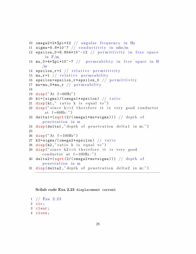
Scilab code Exa 2.23 displacement current

1 // Exa 2 . 2 32 clc;

3 clear;

4 close;

28

5 // g i v e n :6 Ic=10 // conduc t i on c u r r e n t i n ampere7 epsilon_r =1 // r e l a t i v e p e r m i t t i v i t y8 epsilon_0 =8.854*10^ -12 // p e r m i t t i v i t y i n f r e e space9 epsilon=epsilon_r*epsilon_0 // p e r m i t t i v i t y10 sigma =5.8*10^7 // c o n d u c t i v i t y i n mho/m11 disp(”when f =1MHz”)12 f=1 // f r e q u e n c y i n MHz13 f=1*10^6 // f r e q u e n c y i n Hz14 Id=2*%pi*f*epsilon*Ic/sigma // d i s p l a c e m e n t c u r r e n t15 disp(Id,” d i s p l a c e m e n t c u r r e n t when f =1MHz i n A: ”)16 disp(”when f =100MHz”)17 f=100 // f r e q u e n c y i n MHz18 f=100*10^6 // f r e q u e n c y i n Hz19 Id=2*%pi*f*epsilon*Ic/sigma // d i s p l a c e m e n t c u r r e n t20 disp(Id,” d i s p l a c e m e n t c u r r e n t when f =100MHz i n A: ”)

Scilab code Exa 2.25 reachable depth of the sea

1 // Exa 2 . 2 52 clc;

3 clear;

4 close;

5 // g i v e n :6 Em=20 // minimum s i g n a l l e v e l r e q u i r e d f o r v e s s e l

under s ea water i n microV /m7 Em=20*10^ -6 // minimum s i g n a l l e v e l r e q u i r e d f o r

v e s s e l under s ea water i n V/m8 E=100 // e l e c t r i c i n t e n s i t y o f wave i n V/m9 v=3*10^8 // speed o f l i g h t i n m/ s

10 f=4 // f r e q u e n c y i n MHz11 f=4*10^6 // f r e q u e n c y i n Hz12 omega =2* %pi*f // a n g u l a r f r e q u e n c y i n Hz13 sigma=4 // c o n d u c t i v i t y o f s e a water i n mho/m14 epsilon_r =81 // r e l a t i v e p e r m i t t i v i t y

29

15 epsilon_0 =8.854*10^ -12 // p e r m i t t i v i t y i n f r e e space16 epsilon=epsilon_r*epsilon_0 // p e r m i t t i v i t y17 mu_r=1 // r e l a t i v e p e r m e a b i l i t y18 mu_0 =4*%pi *10^( -7) // p e r m e a b i l i t y i n f r e e space19 mu=mu_r*mu_0 // p e r m e a b i l i t y20 k=(sigma)/(omega*epsilon)// r a t i o21 disp(” r a t i o k i s e q u a l to : ”)22 disp(k,” r a t i o : ”)23 disp(”K i s >>1 so s ea water i s a good conduc to r ”)24 eta_1 =377 // i n t r i n s i c impedance i n f r e e space i n

ohm25 alpha_1 =0 // a t t e n u a t i o n c o n s t a n t i n f r e e space i n m

ˆ−126 beta_1=omega/v // phase c o n s t a n t i n mˆ−127 mageta_2=sqrt(omega*mu/sigma) // magnitude o f e t a 2 (

i n t r i n s i c impedance o f s e a water i n ohm)28 argeta_2 =45 // argument o f e t a 2 i n d e g r e e s29 eta_2=mageta_2*cosd(argeta_2)+%i*mageta_2*sind(

argeta_2) // i n t r i n s i c impedance i n complex form (r ∗ co s ( t h e t a )+%i∗ r ∗ s i n ( t h e t a ) )

30 TC=2* eta_2/(eta_1+eta_2) // t r a n s m i s s i o n c o f f i c i e n t31 Et=abs(TC)*E // t r a n s m i t t e d e l e c t r i c f i e l d i n V/m32 alpha_2=sqrt(omega*mu*sigma /2) // a t t e n u a t i o n

c o n s t a n t f o r s e a water i n mˆ−133 // fo rmu la : Et∗ exp(− a l p h a 2 ∗d )=Es34 d=-(1/ alpha_2)*log(Em/Et) // depth i n the s ea tha t

can be r eached by the a e r o p l a n e i n m35 disp(d,” depth i n the s ea tha t can be r eached by the

a e r o p l a n e i n m: ”)36

37

38 // note 1 : the v a l u e o f a l p h a 2 i n book i s 7 . 9 0 5 buti t i s ” 7 . 9 4 ” e x a c t l y c a l c u l a t e d by s c i l a b

39 // note 2 : The c o r r e c t answer o f the Depth ( d ) i s” 1 . 4 10 9 4 ” the answer i n the book i s wrong .

30

Scilab code Exa 2.27 Power per unit area

1 // Exa 2 . 2 72 clc;

3 clear;

4 close;

5 // g i v e n :6 eta_0 =377 // i n t r i n s i c impedance i n f r e e space i n

ohm7 disp(”E=s i n ( omega∗ t−beta ∗ z ) ax+2∗ s i n ( omega∗ t−beta ∗ z

+75) ay // e l e c t r i c f i e l d i n V/m”)8 Ex=1 // magnitude o f Ex9 Ey=2 // magnitude o f Ey10 E=sqrt(Ex^2+Ey^2) // r e s u l t a n t magnitude11 Pav =(1/2)*E^2/( eta_0) // power per u n i t a r ea

conveyed by the wave i n f r e e space12 disp(Pav*1000,” power per u n i t a r ea conveyed by the

wave i n f r e e space i n mW/mˆ 2 : ”)

Scilab code Exa 2.28 average power and maximum energy density of wave

1 // Exa 2 . 2 82 clc;

3 clear;

4 close;

5 // g i v e n :6 epsilon_0 =8.854*10^ -12 // p e r m i t t i v i t y i n f r e e space


/m8 epsilon_r =4 // r e l a t i v e p e r m i t t i v i t y9 mu_r=1 // r e l a t i v e p e r m e a b i l i t y

31

10 epsilon=epsilon_r*epsilon_0 // p e r m i t t i v i t y11 mu=mu_0*mu_r // p e r m e a b i l i t y12 H=5 // magnitude o f magnet i c f i e l d i n mA/m13 H=5*10^ -3 // magnitude o f magnet i c f i e l d i n A/m14 eta=sqrt(mu/epsilon)// i n t r i n s i c impedence i n ohm15 E=H*sqrt(mu/epsilon) // magnitude o f e l e c t r i c f i e l d16 P_av=E^2/(2* eta) // ave rage power17 W_E=epsilon*E^2 // maximum energy d e n s i t y o f the

wave18 disp(P_av *10^6,” Average power i n micro ∗w/mˆ 2 : ”)19 disp(W_E *10^12 ,”maximum energy d e n s i t y o f the wave

i n PJ/mˆ 3 : ”)20

21

22 // note : P av i s = 2 3 5 3 . 7 5 i n book but i t i s 2 3 5 4 . 5 8c o r r e c t l y c a l c u l a t e d by s c i l a b .

Scilab code Exa 2.29 energy density and total energy

1 // Exa 2 . 2 92 clc;

3 clear;

4 close;

5 // g i v e n :6 epsilon_0 =8.854*10^ -12 // p e r m i t t i v i t y i n f r e e space


/m8 epsilon_r =1 // r e l a t i v e p e r m i t t i v i t y9 mu_r=1 // r e l a t i v e p e r m e a b i l i t y10 epsilon=epsilon_r*epsilon_0 // p e r m i t t i v i t y11 mu=mu_0*mu_r // p e r m e a b i l i t y12 E=100* sqrt(%pi) // magnitude o f e l e c t r i c f i e l d i n V/

m13 W_E =(1/2)*epsilon*E^2 // e l e c t r i c ene rgy d e n s i t y o f

32

the wave14 disp(W_E*10^9,” e l e c t r i c ene rgy d e n s i t y o f the wave

i n nJ/mˆ 3 : ”)15 W_H=W_E // as the ene rgy d e n s i t y i s e q u a l to tha t o f

magnet i c f i e l d f o r a pla ‘ ne t r a v e l l i n g wave16 W_T=W_E+W_H // t o t a l ene rgy d e n s i t y17 disp(W_H*10^9,” magnet i c ene rgy d e n s i t y o f wave i n nJ

/mˆ 3 : ”)18 disp(W_T*10^9,” Tota l ene rgy d e n s i t y i n nJ/mˆ 3 : ”)

Scilab code Exa 2.30 transmitted distance of an electromagnetic wave

1 // Exa 2 . 3 02 clc;

3 clear;

4 close;

5 // g i v e n :6 sigma=5 // c o n d u c t i v i t y o f s e a water i n mho/m7 f1=25 // f r e q u e n c y i n kHz8 f1 =25*10^3 // f r e q u e n c y i n Hz9 omega1 =2*%pi*f1 // a n g u l a r f r e q u e n c y i n Hz10 f2=25 // f r e q u e n c y i n MHz11 f2 =25*10^6 // f r e q u e n c y i n Hz12 omega2 =2*%pi*f2 // a n g u l a r f r e q u e n c y i n Hz13 epsilon_r =81 // r e l a t i v e p e r m i t t i v i t y14 epsilon_0 =8.854*10^ -12 // p e r m i t t i v i t y i n f r e e space15 epsilon=epsilon_r*epsilon_0 // p e r m i t t i v i t y16 mu_r=1 // r e l a t i v e p e r m e a b i l i t y17 mu_0 =4*%pi *10^( -7) // p e r m e a b i l i t y i n f r e e space18 mu=mu_r*mu_0 // p e r m e a b i l i t y19 disp(”when f r e q u e n c y =25kHz”)20 alpha_1=omega1*sqrt((mu*epsilon)/2*( sqrt (1+( sigma

^2/( omega1 ^2* epsilon ^2))) -1)) // a t t e n u a t i o nc o n s t a n t when f =25kHz

21 // fo rmu la : exp(−a lpha ∗x ) =0.1

33

22 x1=2.3/ alpha_1 // t r a n s m i t t e d d i s t a n c e i n m23 disp(x1,” t r a n s m i t t e d d i s t a n c e i n m: ”)24 disp(”when f r e q u e n c y =25MHz”)25 alpha_2=omega2*sqrt((mu*epsilon)/2*( sqrt (1+( sigma

^2/( omega2 ^2* epsilon ^2))) -1)) // a t t e n u a t i o nc o n s t a n t when f =25MHz

26 x2=2.3/ alpha_2 // t r a n s m i t t e d d i s t a n c e i n m27 disp(x2,” t r a n s m i t t e d d i s t a n c e i n m: ”)28

29

30 // note : the v a l u e s o f e p s i l o n r =81 and o f mu r=1 f o rs ea water which a r e not g i v e n i n the book .

Scilab code Exa 2.31 incident and reflected magnetic field and reflected electric field

1 // Exa 2 . 3 12 clc;

3 clear;

4 close;

5 // g i v e n :6 E_i=1 // magnitude o f i n c i d e n t e l e c t r i c f i e l d i n mV/

m7 E_i =1*10^ -3 // magnitude o f i n c i d e n t e l e c t r i c f i e l d

i n V/m8 epsilon_0 =8.854*10^ -12 // p e r m i t t i v i t y i n f r e e space


/m10 theta_i =15 // i n c i d e n t a n g l e i n d e g r e e s11 epsilon_r1 =8.5 // r e l a t i v e p e r m i t t i v i t y o f medium 112 mu_r1=1 // r e l a t i v e p e r m e a b i l i t y o f medium 113 epsilon1=epsilon_r1*epsilon_0 // p e r m i t t i v i t y14 mu1=mu_0*mu_r1 // p e r m e a b i l i t y15 eta1=sqrt(mu1/epsilon1) // i n t r i n s i c impedence o f

medium 1 i n ohm

34

16 epsilon2=epsilon_0 // p e r m i t t i v i t y o f medium 217 mu2=mu_0 // p e r m e a b i l i t y o f medium 218 eta2=sqrt(mu2/epsilon2) // i n t r i n s i c impedence o f

medium 2 i n ohm19 // fo rmu la : s i n d ( t h e t a i ) / s i n d ( t h e t a t )=s q r t (

e p s i l o n 2 / e p s i l o n 1 )20 theta_t=asind(sind(theta_i)/(sqrt(epsilon2/epsilon1)

)) // t r a n s m i t t e d a n g l e i n d e g r e e s21 E_r=E_i*(( eta2*cosd(theta_i)-(eta1*cosd(theta_i)))/(

eta2*cosd(theta_i)+eta1*cosd(theta_i))) //r e f l e c t i o n c o f f i c i e n t o f e l e c t r i c f i e l d

22 disp(E_r*1000,” r e f l e c t i o n c o f f i c i e n t o f e l e c t r i cf i e l d i n mV/m: ”)

23 H_i=E_i/eta1 // i n c i d e n t c o f f i c i e n t o f magnet i cf i e l d

24 disp(H_i*10^6,” i n c i d e n t c o f f i c i e n t o f magnet i c f i e l di n micro ∗A/m: ”)

25 H_r=E_r/eta1 // r e f l e c t i o n c o f f i c i e n t o f e l e c t r i cf i e l d

26 disp(H_r*10^6,” r e f l e c t i o n c o f f i c i e n t o f magnet i cf i e l d i n micro ∗A/m: ”)

27

28

29 // note : minute d i f f e r e n c e i n dec ima l answerbetween s c i l a b and book .

Scilab code Exa 2.32 average power density absorbed

1 // Exa 2 . 3 22 clc;

3 clear;

4 close;

5 // g i v e n :6 sigma =5.8*10^7 // c o n d u c t i v i t y i n mho/m7 f=2 // f r e q u e n c y i n MHz

35

8 f=2*10^6 // f r e q u e n c y i n Hz9 omega =2* %pi*f // a n g u l a r f r e q u e n c y i n rad / s e c10 E=2 // magnitude o f e l e c t r i c f i e l d i n mV/m11 E=2*10^ -3 // magnitude o f e l e c t r i c f i e l d i n V/m12 epsilon_0 =8.854*10^ -12 // p e r m i t t i v i t y i n f r e e space


/m14 epsilon_r =1 // r e l a t i v e p e r m i t t i v i t y15 mu_r=1 // r e l a t i v e p e r m e a b i l i t y16 epsilon=epsilon_r*epsilon_0 // p e r m i t t i v i t y17 mu=mu_0*mu_r // p e r m e a b i l i t y18 eta=sqrt(mu*omega/sigma) // i n t r i n s i c impedence i n

ohm19 P_av =(1/2)*E^2/eta // ave rage power d e n s i t y

anbsorbed by copper20 disp(P_av *1000,” ave rage power d e n s i t y anbsorbed by

copper i n mW/mˆ 2 : ”)

36

Chapter 3

RADIATION ANDANTENNAS

Scilab code Exa 3.1 radiation resistance

1 // Exa 3 . 12 clc;

3 clear;

4 close;

5 Lm=poly(0, ’Lm ’ )// d e f i n i n g Lm as lambda6 dl=Lm/40 // d i p o l e l e n g t h7 Rr=80*( %pi)^(2)*(dl/Lm)^2

8 Rr=horner(Rr ,1)

9 disp(Rr,” r a d i a t i o n r e s i s t a n c e o f d i p o l e i n ohm i f d l=Lm/40 : ”)

10 dl=Lm/60 // d i p o l e l e n g t h11 Rr=80*( %pi)^(2)*(dl/Lm)^2

12 Rr=horner(Rr ,1)

13 disp(Rr,” r a d i a t i o n r e s i s t a n c e o f d i p o l e i n ohm i f d l=Lm/60 : ”)

14 dl=Lm/80 // d i p o l e l e n g t h15 Rr=80*( %pi)^(2)*(dl/Lm)^2

16 Rr=horner(Rr ,1)

17 disp(Rr,” r a d i a t i o n r e s i s t a n c e o f d i p o l e i n ohm i f d l

37

=Lm/80 : ”)

Scilab code Exa 3.3 Directivity of half wave dipole

1 //Exa 3 . 32 clc;

3 clear;

4 close;

5 // g i v e n :6 Pr=1 // power i n watt7 I=sqrt(Pr/73) // c u r r e n t i n A8 Eta0 =120*( %pi) // c o n s t a n t9 r=poly(0, ’ r ’ )

10 E_max =60*I/r

11 RI=r^2* E_max ^2/ Eta0 // r a d i a t i o n i n t e n s i t y12 Gd_max =4*( %pi)*(RI)/Pr

13 Gd_max=horner(Gd_max ,1)

14 disp(Gd_max ,” D i r e c t i v i t y o f a h a l f wave d i p o l e : ” )

Scilab code Exa 3.4 Power radiated

1 // Exa3 . 42 clc;

3 clear;

4 close;

5 Rr=300 // r a d i a t i o n r e s i s t a n c e i n ohm6 I=3 // i n A7 // fo rmu la : Pr=I ˆ2∗R8 Pr=I^2*Rr // power r a d i a t e d i n watt9 disp(Pr,” power r a d i a t e d by antenna i n watt s : ”)

38

Scilab code Exa 3.5 effective area of half wave dipole

1 //Exa 3 . 52 clc;

3 close;

4 clear;

5 // g i v e n :6 f=500 // f r e q u e n c y i n mega h e r t z7 f=500*10^6 // f r e q u e n c y i n h e r t z8 c=3*10^8 // speed o f l i g h t i n m/ s9 Gdmax =1.644 // d i r e c t i v i t y o f a h a l f wave d i p o l e

10 lambda=c/f // wave l ength i n meter11 Ae=(( lambda)^2* Gdmax)/(4*( %pi)) // E f f e c t i v e a r ea i n

mˆ212 disp(Ae,” e f f e c t i v e a r ea o f h a l f wave d i p o l e i n mˆ 2 : ”

)

Scilab code Exa 3.6 effective area of hertzian dipole

1 // Exa 3 . 62 clc;

3 clear;

4 close;

5 // g i v e n :6 f=100 // f r e q u e n c y i n Mhz7 f=100*10^6 // f r e q u e n c y i n h e r t z8 c=3*10^8 // speed o f l i g h t i n m/ s9 D=1.5 // d i r e c t i v i t y

10 lambda=c/f // wave l ength i n meter11 Ae=( lambda ^2*D)/(4*( %pi)) // e f f e c t i v e a r ea i n mˆ212 disp(Ae,” E f f e c t i v e a r ea o f h e r t e z i a n d i p o l e i n mˆ 2 :

”)

39

Chapter 4

ANALYSIS OF LINEARARRAYS

Scilab code Exa 4.1 null to null beam width of a broadside array

1 //Exa 4 . 12 clc;

3 clear;

4 close;

5 L=poly(0, ’L ’ ) // D e f i n i n g L as lambda6 l=10*L

7 N=20 // number o f e l e m e n t s8 d=l/N

9 // fo rmu la : BW=(2∗(L/d ) ∗1/N)10 BW1=( horner ((2*L/(N*d)) ,1))

11 disp(BW1 ,” Nul l−to−n u l l BW o f b r o a d s i d e a r r a y i nr a d i a n s when l =10∗L ,N=20: ”)

12 l=50*L




40

18 l=20*L




Scilab code Exa 4.2 null to null beam width of a endfire array

1 //Exa 4 . 22 clc;

3 clear;

4 close;

5 L=poly(0, ’L ’ ) // D e f i n i n g L as lambda6 l=10*L


9 // fo rmu la : BW=(2∗ s q r t ( 2∗ ( L/d ) ∗1/N) )10 BW1 =2* sqrt(horner ((2*L/(N*d)) ,1))

11 disp(BW1 ,” Nul l−to−n u l l BW o f end− f i r e a r r a y i nr a d i a n s when l =10∗L ,N=20: ”)

12 l=50*L



17 disp(BW2 ,” Nul l−to−n u l l BW o f end− f i r e a r r a y i nr a d i a n s when l =50∗L ,N=100: ”)

18 l=20*L



23 disp(BW3 ,” Nul l−to−n u l l BW o f end− f i r e a r r a y i n

41

r a d i a n s when l =20∗L ,N=50: ”)

Scilab code Exa 4.3 null to null beam width and directivity

1 //Exa 4 . 32 clc;

3 clear;

4 close;

5 f=6 // f r e q u e n c y i n GHz6 f=6*10^9 // f r e q u e n c y i n Hz7 c=3*10^8 // speed o f l i g h t i n m/ s8 l=10 // a r r a y l e n g t h i n meter9 lambda=c/f // wave l ength i n meter

10 // fo rmu la : BWFN = 2∗ lambda / l11 BWFN = 2*( lambda/l) // band width i n r a d i a n s12 disp(BWFN ,” n u l l −to−n u l l Beamwidth o f broad s i d e

a r r a y i n r a d i a n s : ”)13 D=2*(l/lambda) // d i r e c t i v i t y14 disp(D,” D i r e c t i v i t y : ”)

Scilab code Exa 4.4 Progressive phase shift and array length

1 //Exa 4 . 42 clc;

3 clear;

4 close;

5 // g i v e n :6 f=10 // f r e q u e n c y i n Ghz7 f=10*10^9 // f r e q u e n c y i n h e r t z8 c=3*10^8 // speed o f l i g h t i n m/ s9 lambda=c/f // wave l ength i n meter

10 N=50 // number o f e l e m e n t s11 d=0.5* lambda // e l ement s p a c i n g i n meter

42

12 Beta =2*( %pi)/lambda // phase s h i f t13 alpha=Beta*d // p r o g r e s s i v e phase s h i f t i n r a d i a n s14 l=N*d // Araay l e n g t h i n meter15 disp(alpha ,” p r o g r e s s i v e phase s h i f t i n r a d i a n s : ”)16 disp(l,” Array l e n g t h i n meter ”)

Scilab code Exa 4.5 null to null and half power beam width and directivity

1 //Exa 4 . 52 clc;

3 clear;

4 close;

5 // g i v e n :6 N=100 // no . o f e l e m e n t s7 Lm=poly(0, ’Lm ’ ) // d e f i n i n g Lm as lambda8 d=0.5* Lm

9 l=N*d // a r r a y l e n g t h10 B.W.F.N = 114.6 /(l/Lm) // beam width i n d e g r e e s11 B.W.F.N=horner(B.W.F.N,1)

12 disp(B.W.F.N ,” n u l l −to−n u l l beamwidth i n d e g r e e s : ”)13 H.P.B.W = B.W.F.N/2 // h a l f power beam width i n

d e g r e e s14 disp(H.P.B.W ,” h a l f power beamwidth i n d e g r e e s : ”)15 D1=2*(l/Lm) // d i r e c t i v i t y o f broad s i d e a r r a y16 D1=horner(D1 ,1)

17 D2=4*(l/Lm) // d i r e c t i v i t y o f end f i r e a r r a y18 D2=horner(D2 ,1)

19 disp(D1,” d i r e c t i v i t y o f broad s i d e a r r a y : ”)20 disp(D2,” d i r e c t i v i t y o f end f i r e a r r a y : ”)21

22 // note : answer i n the book i s mis−pr in t ed , the HPBWi s not 1 1 . 4 6 i t shou ld be 1 . 1 4 6 d e g r e e s .

23

24 // note : m i s p r i n t i n second s t e p o f pa r t a i n bookc o r r e c t i s l=N∗d =100∗0.5∗ lambda=50∗ lambda

43

Scilab code Exa 4.9 relative excitation levels

1 // Exa 4 . 92 clc;

3 clear;

4 close;

5 // g i v e n :6 // fo rmu la : combinat ion ( n , r ) =( f a c t o r i a l ( n ) ) /(

f a c t o r i a l ( r ) ∗ f a c t o r i a l ( n−r ) )7 disp(”when n=2”)8 n=2

9 a_0=factorial (1)/factorial (0)*factorial (1) //r e l a t i v e e x c i t a t i o n l e v e l 1


11 disp(( string(a_0)+” ”+string(a_1)),” r e l a t i v ee x c i t a t i o n l e v e l s o f b i n o m i a l a r r a y at n=2: ”)

12 disp(”when n=3”)13 n=3


15 a_0 =2*a_1 // r e l a t i v e e x c i t a t i o n l e v e l 116 disp(( string(a_1)+” ”+string(a_0)+” ”+string(a_1)),”

r e l a t i v e e x c i t a t i o n l e v e l s o f b i n o m i a l a r r a y at n=3: ”)

Scilab code Exa 4.10 basic and actual transmission loss

1 // Exa 4 . 1 02 clc;

3 clear;

44

4 close;

5 // g i v e n :6 d=30 // s e p a r a t i o n d i s t a n c e i n meter7 f=10 // f r e q u e n c y i n mega h e r t z8 f=10*10^6 // f r e q u e n c y i n h e r t z9 c=3*10^8 // speed o f l i g h t i n m/ s10 lambda=c/f // wave l ength i n meter11 Gt=1.65 // t r a n s m i t t i n g ga in i n dB12 Gr=1.65 // r e c e i v i n g ga in i n dB13 // b a s i c t r a n s m i s s i o n l o s s :14 // fo rmu la : Lb=10∗ l o g ( ( ( 4 ∗ ( %pi ) ∗d ) ˆ2/( lambda ) ˆ2) )15 Lb=10* log10 ((4*( %pi)*d)^2/( lambda)^2) // b a s i c

t ransmmis ion l o s s i n dB16 disp(Lb,” b a s i c t ransmmis ion l o s s i n dB : ”)17 // a c t u a l t r a n s m i s s i o n l o s s :18 La=Lb-Gt-Gr // a c t u a l t r a n s m i s s o n l o s s i n dB19 disp(La,” a c t u a l t r a n s m i s s o n l o s s i n dB : ”)

Scilab code Exa 4.11 basic transmission loss

1 //Exa 4 . 1 12 clc;

3 clear;

4 close;

5 //when f r e q u e n c y =0.3GHz6 // g i v e n :7 f=0.3 // f r e q u e n c y i n Ghz8 f=0.3*10^9 // f r e q u e n c y i n h e r t z9 c=3*10^8 // speed o f l i g h t i n m/ s

10 lambda=c/f // wave l ength i n meter11 d1=1.6 // i n Km12 d1 =1.6*10^3 // i n meter13 // fo rmu la : Lb=20∗ l o g 1 0 ( ( 4 ∗ ( %pi ) ∗d ) /( lambda ) )14 Lb1 =20* log10 (4* %pi*d1/lambda) // b a s i c t r a n s m i s s i o n

l o s s i n dB

45

15 disp(Lb1 ,” b a s i c t r a n s m i s s i o n l o s s i n dB when d=1.6Km, f =0.3GHz : ”)

16 d2=16 // i n Km17 d2 =16*10^3 // i n meter18 // fo rmu la : Lb=20∗ l o g 1 0 ( ( 4 ∗ ( %pi ) ∗d ) /( lambda ) )19 Lb2 =20* log10 (4* %pi*d2/lambda) // b a s i c t r a n s m i s s i o n

l o s s i n dB20 disp(Lb2 ,” b a s i c t r a n s m i s s i o n l o s s i n dB when d=16Km,

f =0.3GHz : ”)21 d3=160 // i n Km22 d3 =160*10^3 // i n meter23 // fo rmu la : Lb=20∗ l o g 1 0 ( ( 4 ∗ ( %pi ) ∗d ) /( lambda ) )24 Lb3 =20* log10 (4* %pi*d3/lambda) // b a s i c t r a n s m i s s i o n

l o s s i n dB25 disp(Lb3 ,” b a s i c t r a n s m i s s i o n l o s s i n dB when d=160Km

, f =0.3GHz : ”)26 d4=320 // i n Km27 d4 =320*10^3 // i n meter28 // fo rmu la : Lb=20∗ l o g 1 0 ( ( 4 ∗ ( %pi ) ∗d ) /( lambda ) )29 Lb4 =20* log10 (4* %pi*d4/lambda) // b a s i c t r a n s m i s s i o n


, f =0.3GHz : ”)31 // when f r e q u e n c y i s 3Ghz32 // g i v e n :33 f=3 // f r e q u e n c y i n Ghz34 f=3*10^9 // f r e q u e n c y i n h e r t z35 c=3*10^8 // speed o f l i g h t i n m/ s36 lambda=c/f // wave l ength i n meter37 d1=1.6 // i n Km38 d1 =1.6*10^3 // i n meter39 // fo rmu la : Lb=20∗ l o g 1 0 ( ( 4 ∗ ( %pi ) ∗d ) /( lambda ) )40 Lb1 =20* log10 (4* %pi*d1/lambda) // b a s i c t r a n s m i s s i o n

l o s s i n dB41 disp(Lb1 ,” b a s i c t r a n s m i s s i o n l o s s i n dB when d=1.6Km

, f =3GHz : ”)42 d2=16 // i n Km43 d2 =16*10^3 // i n meter

46

44 // fo rmu la : Lb=20∗ l o g 1 0 ( ( 4 ∗ ( %pi ) ∗d ) /( lambda ) )45 Lb2 =20* log10 (4* %pi*d2/lambda) // b a s i c t r a n s m i s s i o n

l o s s i n dB46 disp(Lb2 ,” b a s i c t r a n s m i s s i o n l o s s i n dB when d=16Km,

f =3GHz : ”)47 d3=160 // i n Km48 d3 =160*10^3 // i n meter49 // fo rmu la : Lb=20∗ l o g 1 0 ( ( 4 ∗ ( %pi ) ∗d ) /( lambda ) )50 Lb3 =20* log10 (4* %pi*d3/lambda) // b a s i c t r a n s m i s s i o n


, f =3GHz : ”)52 d4=320 // i n Km53 d4 =320*10^3 // i n meter54 // fo rmu la : Lb=20∗ l o g 1 0 ( ( 4 ∗ ( %pi ) ∗d ) /( lambda ) )55 Lb4 =20* log10 (4* %pi*d4/lambda) // b a s i c t r a n s m i s s i o n


, f =3GHz : ”)

Scilab code Exa 4.12 Actual transmission loss

1 //Exa 4 . 1 22 clc;

3 clear;

4 close;

5 // g i v e n :6 Gt=10 // t r a n s m i s s i o n ga in i n dB7 Gr=10 // r e c e i v i n g ga in i n dB8 //when f r e q u e n c y =0.3GHz9 // g i v e n :10 f=0.3 // f r e q u e n c y i n Ghz11 f=0.3*10^9 // f r e q u e n c y i n h e r t z12 c=3*10^8 // speed o f l i g h t i n m/ s13 lambda=c/f // wave l ength i n meter

47

14 d1=1.6 // i n Km15 d1 =1.6*10^3 // i n meter16 // fo rmu la : Lb=20∗ l o g 1 0 ( ( 4 ∗ ( %pi ) ∗d ) /( lambda ) )17 Lb1 =20* log10 (4* %pi*d1/lambda) // b a s i c t r a n s m i s s i o n

l o s s i n dB18 La1=Lb1 -Gt-Gr // Actua l t r a n s m i s s i o n l o s s i n dB19 disp(La1 ,” Actua l t r a n s m i s s i o n l o s s i n dB when d=1.6

Km, f =0.3GHz : ”)20 d2=16 // i n Km21 d2 =16*10^3 // i n meter22 // fo rmu la : Lb=20∗ l o g 1 0 ( ( 4 ∗ ( %pi ) ∗d ) /( lambda ) )23 Lb2 =20* log10 (4* %pi*d2/lambda) // b a s i c t r a n s m i s s i o n

l o s s i n dB24 La2=Lb2 -Gt-Gr // Actua l t r a n s m i s s i o n l o s s i n dB25 disp(La2 ,” Actua l t r a n s m i s s i o n l o s s i n dB when d=16Km

, f =0.3GHz : ”)26 d3=160 // i n Km27 d3 =160*10^3 // i n meter28 // fo rmu la : Lb=20∗ l o g 1 0 ( ( 4 ∗ ( %pi ) ∗d ) /( lambda ) )29 Lb3 =20* log10 (4* %pi*d3/lambda) // b a s i c t r a n s m i s s i o n

l o s s i n dB30 La3=Lb3 -Gt-Gr // Actua l t r a n s m i s s i o n l o s s i n dB31 disp(La3 ,” Actua l t r a n s m i s s i o n l o s s i n dB when d=160

Km, f =0.3GHz : ”)32 d4=320 // i n Km33 d4 =320*10^3 // i n meter34 // fo rmu la : Lb=20∗ l o g 1 0 ( ( 4 ∗ ( %pi ) ∗d ) /( lambda ) )35 Lb4 =20* log10 (4* %pi*d4/lambda) // b a s i c t r a n s m i s s i o n


Km, f =0.3GHz : ”)38 // when f r e q u e n c y i s 3Ghz39 // g i v e n :40 f=3 // f r e q u e n c y i n Ghz41 f=3*10^9 // f r e q u e n c y i n h e r t z42 c=3*10^8 // speed o f l i g h t i n m/ s43 lambda=c/f // wave l ength i n meter

48

44 d1=1.6 // i n Km45 d1 =1.6*10^3 // i n meter46 // fo rmu la : Lb=20∗ l o g 1 0 ( ( 4 ∗ ( %pi ) ∗d ) /( lambda ) )47 Lb1 =20* log10 (4* %pi*d1/lambda) // b a s i c t r a n s m i s s i o n

l o s s i n dB48 La1=Lb1 -Gt-Gr // Actua l t r a n s m i s s i o n l o s s i n dB49 disp(La1 ,” Actua l t r a n s m i s s i o n l o s s i n dB when d=1.6

Km, f =3GHz : ”)50 d2=16 // i n Km51 d2 =16*10^3 // i n meter52 // fo rmu la : Lb=20∗ l o g 1 0 ( ( 4 ∗ ( %pi ) ∗d ) /( lambda ) )53 Lb2 =20* log10 (4* %pi*d2/lambda) // b a s i c t r a n s m i s s i o n

l o s s i n dB54 La2=Lb2 -Gt-Gr // Actua l t r a n s m i s s i o n l o s s i n dB55 disp(La2 ,” Actua l t r a n s m i s s i o n l o s s i n dB when d=16Km

, f =3GHz : ”)56 d3=160 // i n Km57 d3 =160*10^3 // i n meter58 // fo rmu la : Lb=20∗ l o g 1 0 ( ( 4 ∗ ( %pi ) ∗d ) /( lambda ) )59 Lb3 =20* log10 (4* %pi*d3/lambda) // b a s i c t r a n s m i s s i o n


Km, f =3GHz : ”)62 d4=320 // i n Km63 d4 =320*10^3 // i n meter64 // fo rmu la : Lb=20∗ l o g 1 0 ( ( 4 ∗ ( %pi ) ∗d ) /( lambda ) )65 Lb4 =20* log10 (4* %pi*d4/lambda) // b a s i c t r a n s m i s s i o n


Km, f =3GHz : ”)

Scilab code Exa 4.13 receiving power

49

1 //Exa 4 . 1 32 clc;

3 clear;

4 close;

5 // g i v e n :6 Wt=15 // r a d a i t e d power i n watt7 f=60 // i n MHz8 f=60*10^6 // i n Hz9 d=10 // i n m10 c=3*10^8 // i n m/ s11 lambda=c/f // i n meter12 Gt=1.64 // t r a n s m i t t i n g ga in i n dB13 Gr=1.64 // r e c e i v i n g ga in i n dB14 Wr=(Wt*Gt*Gr*( lambda)^2/(4*( %pi)*d)^2) // r e c e i v i n g

power i n watt15 disp(Wr*1000,” r e c e i v i n g power i n mW: ”)

50

Chapter 6

HF VHF AND UHFANTEENAS

Scilab code Exa 6.1 Designing of a rhombic antenna

1 //Exa 6 . 12 clc;

3 clear;

4 close;

5 // g i v e n :6 f=30 // f r e q u e n c y i n MHz7 f=30*10^6 // f r e q u e n c y i n Hz8 c=3*10^8 // speed o f l i g h t i n m/ s9 lambda=c/f // wave l ength i n meter

10 Delta =30 // a n g l e o f e l e v a t i o n i n Degree s11 H=lambda /(4* sind(Delta)) // Rhombic h e i g h t i n m12 phi=90-Delta // t i l t a n g l e i n Degree s13 l=lambda /(2*( cosd(phi)^2)) // w i r e l e n g t h i n m14 disp(H,” Rhombic h e i g h t i n m: ”)15 disp(phi ,” T i l t a n g l e i n Degree s : ”)16 disp(l,” l e n g t h o f w i r e i n meter : ”)

51


1 //Exa 6 . 22 clc;

3 clear;

4 close;


10 Delta =10 // a n g l e o f e l e v a t i o n i n Degree s11 H=lambda /(4* sind(Delta)) // Rhombic h e i g h t i n m12 phi=90-Delta // t i l t a n g l e i n Degree s13 l=lambda /(2*( cosd(phi)^2)) // w i r e l e n g t h i n m14 disp(H,” Rhombic h e i g h t i n m: ”)15 disp(phi ,” T i l t a n g l e i n Degree s : ”)16 disp(l,” l e n g t h o f w i r e i n meter : ”)


1 //Exa 6 . 32 clc;

3 clear;

4 close;


10

11 disp(” f o r De l ta =10 d e g r e e s ”)12

13 Delta1 =10 // a n g l e o f e l e v a t i o n i n Degree s14 H1=lambda /(4* sind(Delta1)) // Rhombic h e i g h t i n m

52

15 phi1=90- Delta1 // t i l t a n g l e i n Degree s16 l1=lambda /(2*( cosd(phi1)^2)) // w i r e l e n g t h i n m17 disp(H1,” Rhombic h e i g h t i n m: ”)18 disp(phi1 ,” T i l t a n g l e i n Degree s : ”)19 disp(l1,” l e n g t h o f w i r e i n meter : ”)20


23 Delta2 =15 // a n g l e o f e l e v a t i o n i n Degree s24 H2=lambda /(4* sind(Delta2)) // Rhombic h e i g h t i n m25 phi2=90- Delta2 // t i l t a n g l e i n Degree s26 l2=lambda /(2*( cosd(phi2)^2)) // w i r e l e n g t h i n m27 disp(H2,” Rhombic h e i g h t i n m: ”)28 disp(phi2 ,” T i l t a n g l e i n Degree s : ”)29 disp(l2,” l e n g t h o f w i r e i n meter : ”)30






53





73 Delta7 =40 // a n g l e o f e l e v a t i o n i n Degree s74 H7=lambda /(4* sind(Delta7)) // Rhombic h e i g h t i n m75 phi7=90- Delta7 // t i l t a n g l e i n Degree s76 l7=lambda /(2*( cosd(phi7)^2)) // w i r e l e n g t h i n m77 disp(H7,” Rhombic h e i g h t i n m: ”)78 disp(phi7 ,” T i l t a n g l e i n Degree s : ”)79 disp(l7,” l e n g t h o f w i r e i n meter : ”)

Scilab code Exa 6.4 Design parameters of rhombic anteena

1 //Exa 6 . 42 clc;

3 clear;

4 close;

5 // g i v e n :

54

6 f=30 // f r e q u e n c y i n MHz7 f=30*10^6 // f r e q u e n c y i n Hz8 c=3*10^8 // speed o f l i g h t i n m/ s9 K=0.74 // c o n s t a n t10 lambda=c/f // i n meter11 Delta =30 // a n g l e o f e l e v a t i o n i n Degree s12 H=lambda /(4* sind(Delta)) // Rhombic h e i g h t i n m13 phi=90-Delta // t i l t a n g l e i n Degree s14 l=( lambda /(2*( cosd(phi)^2)))*K // w i r e l e n g t h i n m15 disp(H,” Rhombic h e i g h t i n m: ”)16 disp(phi ,” T i l t a n g l e i n Degree s : ”)17 disp(l,” l e n g t h o f w i r e i n meter : ”)

Scilab code Exa 6.5 Design parameters of rhombic anteena

1 //Exa 6 . 52 clc;

3 clear;

4 close;

5 // g i v e n :6 f=20 // f e r q u e n c y i n MHz7 f=20*10^6 // f r e q u e n c y i n Hz8 c=3*10^8 // speed o f l i g h t i n m/ s9 K=0.74 // c o n s t a n t

10 lambda=c/f // wave l ength i n meter11 Delta =20 // a n g l e o f e l e v a t i o n i n Degree s12 H=lambda /(4* sind(Delta)) // Rhombic h e i g h t i n m13 phi=90-Delta // t i l t a n g l e i n Degree s14 l=( lambda /(2*( cosd(phi)^2)))*K // w i r e l e n g t h i n m15 disp(H,”Rhombic h e i g h t i n m: ”)16 disp(phi ,” T i l t a n g l e i n Degree s : ”)17 disp(l,” l e n g t h o f w i r e i n meter : ”)

55

Scilab code Exa 6.6 Design a three element yagi uda antenna

1 //Exa 6 . 62 clc;

3 clear;

4 close;

5 // g i v e n :6 f_MHz =172 // f r e q u e n c y i n MHz7 c=3*10^8 // speed o f l i g h t i n m/ s8 lambda=c/f_MHz // wave l ength i n m9 La=478/ f_MHz // l e n g t h o f d r i v e n e l ement i n f e e t10 Lr=492/ f_MHz // l e n g t h o f r e f l e c t o r i n f e e t11 Ld =461.5/ f_MHz // l e n g t h o f d i r e c t o r i n f e e t12 S=142/ f_MHz // e l ement s p a c i n g i n f e e t13 disp(La,” l e n g t h o f d r i v e n e l ement i n f e e t : ”)14 disp(Lr,” l e n g t h o f r e f l e c t o r i n f e e t : ”)15 disp(Ld,” l e n g t h o f d i r e c t o r i n f e e t : ”)16 disp(S,” e l ement s p a c i n g i n f e e t : ”)

Scilab code Exa 6.7 Designing of a six element yagi uda antenna

1 // Exa6 . 72 clc;

3 clear;

4 close;

5 // g i v e n :6 G=12 // r e q u i r e d ga in i n dB7 f=200 // f r e q u e n c y i n MHz8 f=200*10^6 // f r e q u e n c y i n Hz9 c=3*10^8 // speed o f l i g h t i n m/ s

10 lambda=c/f // wave l ength i n m11 La =0.46* lambda // l e n g t h o f d r i v e n e l ement i n m (

note : i n book La i s g i v e n 0 . 4 1 6∗ lambda m i s p r i n t )12 Lr =0.475* lambda // l e n g t h o f r e f l e c t o r i n m13 Ld1 =0.44* lambda // l e n g t h o f d i r e c t o r 1 i n m

56

14 Ld2 =0.44* lambda // l e n g t h o f d i r e c t o r 2 i n m15 Ld3 =0.43* lambda // l e n g t h o f d i r e c t o r 3 i n m16 Ld4 =0.40* lambda // l e n g t h o f d i r e c t o r 4 i n m17 SL =0.25* lambda // s p a c i n g between r e f l e c t o r and

d r i v e r i n m18 Sd =0.31* lambda // s p a c i n g d i r e c t o r and d r i v i n g

e l ement i n m19 d=0.01* lambda // d iamete r o f e l e m e n t s i n m20 l=1.5* lambda // l e n g t h o f a r r a y i n m21 disp(La,” l e n g t h o f d r i v e n e l ement i n m: ”)22 disp(Lr,” l e n g t h o f r e f l e c t o r i n m: ”)23 disp(Ld1 ,” l e n g t h o f d i r e c t o r 1 i n m: ”)24 disp(Ld2 ,” l e n g t h o f d i r e c t o r 2 i n m: ”)25 disp(Ld3 ,” l e n g t h o f d i r e c t o r 3 i n m: ”)26 disp(Ld4 ,” l e n g t h o f d i r e c t o r 4 i n m: ”)27 disp(SL,” s p a c i n g between r e f l e c t o r and d r i v e r i n m: ”

)

28 disp(Sd,” s p a c i n g d i r e c t o r and d r i v i n g e l ement i n m: ”)

29 disp(d,” d iamete r o f e l e m e n t s i n m: ”)30 disp(l,” l e n g t h o f a r r a y i n m: ”)

Scilab code Exa 6.8 Designing of a long periodic antenna

1 //Exa 6 . 82 clc;

3 clear;

4 close;

5 // g i v e n :6 G=9 // r e q u i r e d ga in i n dB7 f_l =125 // l o w e s t f r e q u e n c y i n MHz8 f_l =125*10^6 // l o w e s t f r e q u e n c y i n Hz9 f_h =500 // h i g h e s t f r e q u e n c y i n MHz

10 f_h =500*10^6 // l o w e s t f r e q u e n c y i n Hz11 c=3*10^8 // speed o f l i g h t i n m/ s

57

12 lambda_l=c/f_l // l o n g e s t wave l ength i n m13 lambda_s=c/f_h // s h o r t e s t wave l ength i n m14 tau =0.861 // s c a l i n g f a c t o r15 sigma =0.162 // s p a c i n g f a c t o r16 alpha =2* atand ((1-tau)/(4* sigma)) // wedge a n g l e i n

Degree s17 L1=lambda_l /2 // i n m18 L2=tau*L1 // i n m19 L3=tau*L2 // i n m20 L4=tau*L3 // i n m21 L5=tau*L4 // i n m22 L6=tau*L5 // i n m23 L7=tau*L6 // i n m24 L8=tau*L7 // i n m25 L9=tau*L8 // i n m26 L10=tau*L9 // i n m27 L11=tau*L10 // i n m28

29 // e l ement s p a c i n g r e l a t i o n30 // fo rmu la : sn=2∗ s igma ∗Ln31 S1=2* sigma*L1 // i n m32 S2=2* sigma*L2 // i n m33 S3=2* sigma*L3 // i n m34 S4=2* sigma*L4 // i n m35 S5=2* sigma*L5 // i n m36 S6=2* sigma*L6 // i n m37 S7=2* sigma*L7 // i n m38 S8=2* sigma*L8 // i n m39 S9=2* sigma*L9 // i n m40 S10 =2* sigma*L10 // i n m41 S11 =2* sigma*L11 // i n m42

43

44 disp(” d e s i g n i n g o f log−p e r i o d i c antenna : ”)45

46 disp(L1,”L1 i n m: ”)47 disp(L2,”L2 i n m: ”)48 disp(L3,”L3 i n m: ”)

58

49 disp(L4,”L4 i n m: ”)50 disp(L5,”L5 i n m: ”)51 disp(L6,”L6 i n m: ”)52 disp(L7,”L7 i n m: ”)53 disp(L8,”L8 i n m: ”)54 disp(L9,”L9 i n m: ”)55 disp(L10 ,”L10 i n m: ”)56 disp(L11 ,”L11 i n m: ”)57

58 disp(” e l e m e n t s s p a c i n g r e l a t i o n : ”)59 disp(S1,”S1 i n m: ”)60 disp(S2,”S2 i n m: ”)61 disp(S3,”S3 i n m: ”)62 disp(S4,”S4 i n m: ”)63 disp(S5,”S5 i n m: ”)64 disp(S6,”S6 i n m: ”)65 disp(S7,”S7 i n m: ”)66 disp(S8,”S8 i n m: ”)67 disp(S9,”S9 i n m: ”)68 disp(S10 ,” S10 i n m: ”)69 disp(S11 ,” S11 i n m: ”)

Scilab code Exa 6.9 induced voltage in a loop antenna

1 //Exa 6 . 92 clc;

3 clear;

4 close;

5 // g i v e n :6 E_rms =10 // e l e c t r i c f i e l d i n mV/m7 E_rms =10*10^ -3 // e l e c t r i c f i e l d i n V/m8 f=2 // f r e q u e n c y i n MHz9 f=2*10^6 // f r e q u e n c y i n Hz

10 N=10 // number o f t u r n s11 phi=0 // a n g l e between the p l ane o f l o op and

59

d i r e c t i o n o f i n c i d e n t wave i n Degree s12 S=1.4 // a r ea o f l o op antenna i n mˆ213 c=3*10^8 // speed o f l i g h t i n m/ s14 lambda=c/f // wave l ength i n m15 E_max=sqrt (2)*E_rms // e l e c t r i c f i e l d i n V/m16 V_rms =(2* %pi*E_max*S*N/lambda)*cosd(phi) // induced

v o l t a g e17 disp(V_rms *1000,” induced v o l t a g e i n mV: ”)

Scilab code Exa 6.10 radiation resistance of a loop antenna

1 // Exa6 . 1 02 clc;

3 clear;

4 close;

5 // g i v e n :6 D=0.5 // d iamete r o f l o op antenna i n m7 a=D/2 // r a d i u s o f l o op antenna i n m8 f=1 // f r e q u e n c y i n MHz9 f=1*10^6 // f r e q u e n c y i n Hz

10 c=3*10^8 // speed o f l i g h t i n m/ s11 lambda=c/f // wave l ength i n m12 Rr =3720*(a/lambda) // r a d i a t i o n r e s i s t a n c e o f l o op

antenna i n ohm13 disp(Rr,” r a d i a t i o n r e s i s t a n c e o f l o op antenna i n ohm

: ”)

Scilab code Exa 6.11 Directivity of a loop antenna

1 //Exa 6 . 1 12 clc;

3 clear;

4 close;

60

5 // g i v e n :6 a=0.5 // r a d i u s o f l o op antenna i n m7 f=0.9 // f r e q u e n c y i n MHz8 f=0.9*10^6 // f r e q u e n c y i n Hz9 c=3*10^8 // speed o f l i g h t i n m/ s10 lambda=c/f // wave l ength i n m11 k=(2* %pi*a)/lambda // c o n s t a n t12 disp(” the v a l u e o f k i s : ”)13 disp(k)

14 disp(” s i n c e , k<1/3”)15 disp(”So D i r e c t i v i t y o f l o op antenna i s D=1.5 ”)

Scilab code Exa 6.13 Directivity and radiation resistance of a loop antenna

1 //Exa 6 . 1 32 clc;

3 clear;

4 close;

5 Lm=poly(0, ’Lm ’ ) // d e f i n i n g Lm as lambda6 d=1.5* Lm // d iamete r o f antenna i n m7 a=d/2 // r a d i u s o f antenna i n m8 // fo rmu la : Rr=3720∗( a/Lm)9 Rr =3720*(a/Lm) // r a d i a t i o n r e s i s t a n c e o f l o op

antenna i n ohm10 Rr=horner(Rr ,1)

11 // fo rmu la : D=4.25∗ ( a/Lm)12 D=4.25*(a/Lm)// D i r e c t i v i t y o f the l oop antenna13 D=horner(D,1)

14 disp(Rr,” r a d i a t i o n r e s i s t a n c e o f the l oop antenna i nohm : ”)

15 disp(D,” D i r e c t i v i t y o f the l oop antenna : ”)

Scilab code Exa 6.14 array length number of elements and null to null beam width

61

1 //Exa 6 . 1 42 clc;

3 clear;

4 close;

5 // g i v e n :6 Gp=28 // power ga in7 Lm=poly(0, ’Lm ’ ) // d e f i n i n g Lm as lambda8 d=Lm/2 // l e n g t h o f d i p o l e9 // fo rmu la : Gp=4∗(L/ lambda )10 L=Gp*Lm/4 // a r r a y l e n g t h11 disp(L,” a r r a y l e n g t h ( where Lm i s wave l ength i n m) : ”)12 N=7*2 // Number o f e l e m e n t s i n the a r r a y when spaced

at lambda /213 disp(N,”Number o f e l e m e n t s i n the a r r a y when spaced

at lambda / 2 : ”)14 // fo rmu la : B .W=2∗ s q r t ( ( 2∗/N) ∗ ( lambda /d ) )15 BW=2* sqrt(horner ((2*Lm/(N*d)) ,1)) // n u l l −to−n u l l

beam width i n r a d i a n s16 BW_d=BW *180/ %pi // n u l l −to−n u l l beam width i n

d e g r e e s17 disp(BW_d ,” n u l l −to−n u l l beam width i n d e g r e e s : ”)18

19

20

21 // Answer o f n u l l −to−n u l l beam width i n d e g r e e s i srounded−o f f i n book .


1 //Exa 6 . 1 52 clc;

3 clear;

4 close;

5 // g i v e n :6 S=0.05 // s p a c i n g i n m

62

7 Dh=0.1 // d iamete r o f h e l i c a l antenna i n m8 N=20 // number o f t u r n s9 f=1000 // f r e q u e n c y i n MHz10 f=1000*10^6 // f r e q u e n c y i n MHz11 c=3*10^8 // speed o f l i g h t i n m/ s12 lambda=c/f // wave l ength i n m13 C=%pi*Dh // c i r c u m f r e n c e o f h e l i x i n m14 La=N*S // a x i a l l e g t h i n m15 phi_not =(115*( lambda ^(3/2))/(C*sqrt(La))) // B .W. F .N

. , n u l l −to−n u l l beamwidth o f main beam i nD e g r e e s s

16 phi =(52* lambda ^(3/2) /(C*sqrt(La))) // H. P .B .W, h a l fpower beamwidth i n D e g r e e s s

17 D=(15*N*C^2*S/( lambda)^3) // D i r e c t i v i t y18 disp(phi_not ,”B .W. F .N. , n u l l −to−n u l l beamwidth o f

main beam i n Degree s : ”)19 disp(phi ,”H. P .B .W, h a l f power beamwidth i n Degree s : ”

)

20 disp(D,” D i r e c t i v i t y : ”)

63

Chapter 7

MICROWAVE ANTENNAS

Scilab code Exa 7.1 null to null and half power beam width of a paraboloid reflector

1 //Exa 7 . 12 clc;

3 clear;

4 close;

5 // g i v e n :6 D=2 // Diameter o f p a r a b o l o i d r e f l e c t o r i n m7 c=3*10^8 // speed o f l i g h t i n m/ s8 f=5 // f r e q u e n c y i n GHz9 f=5*10^9 // f r e q u e n c y i n Hz

10 lambda=c/f // wave l ength i n m11 BWFN =140*( lambda/D) // n u l l −to−n u l l beamwidth i n

d e g r e e s12 HPBW =70*( lambda/D) // h a l f power beamwidth i n

d e g r e e s13 disp(BWFN ,” n u l l −to−n u l l beamwidth i n d e g r e e s : ”)14 disp(HPBW ,” h a l f power beamwidth i n d e g r e e s : ”)

Scilab code Exa 7.2 gain of the paraboloid reflector antenna

64

1 //Exa 7 . 22 clc;

3 clear;

4 close;

5 // g i v e n :6 D=2 // mouth d iamete r o f p a r a b o l o i d r e f l e c t o r i n m7 c=3*10^8 // speed o f l i g h t i n m/ s8 f=5 // f r e q u e n c y i n GHz9 f=5*10^9 // f r e q u e n c y i n Hz

10 lambda=c/f // wave l ength i n m11 G=6.4*(D/lambda)^2 // power ga in o f p a r a b o l o i d12 G_p =10* log10(G) // power ga in i n dB13 disp(G_p ,” power ga in i n dB : ”)

Scilab code Exa 7.3 band width between first null and half power points

1 //Exa 7 . 32 clc;

3 clear;

4 close;

5 // g i v e n :6 D_a =0.15 // mouth Diameter o f p a r a b o l o i d i n m7 c=3*10^8 // speed o f l i g h t i n m/ s8 f=10 // f r e q u e n c y i n GHz9 f=10*10^9 // f r e q u e n c y i n Hz

10 lambda=c/f // wave l ength i n m11 BWFN =140*( lambda/D_a) // n u l l −to−n u l l beamwidth i n

d e g r e e s12 HPBW =70*( lambda/D_a) // h a l f power beamwidth i n

d e g r e e s13 disp(BWFN ,” n u l l −to−n u l l beamwidth i n d e g r e e s : ”)14 disp(HPBW ,” h a l f power beamwidth i n d e g r e e s : ”)15 G_p =6.4*( D_a/lambda)^2 // power ga in o f p a r a b o l o i d16 G_p =10* log10(G_p) // power ga in i n dB17 disp(G_p ,” power ga in i n dB”)

65

Scilab code Exa 7.4 Power gain in Decibels

1 //Exa 7 . 42 clc;

3 clear;

4 close;

5 // g i v e n :6 D_a =1.8 // mouth d iamete r o f p a r a b o l o i d r e f l e c t o r i n

m7 c=3*10^8 // speed o f l i g h t i n m/ s8 f=2 // f r e q u e n c y i n GHz9 f=2*10^9 // f r e q u e n c y i n Hz

10 lambda=c/f // wave l ength i n m11 G_p =6.4*( D_a/lambda)^2 // power ga in o f p a r a b o l o i d12 G_p =10* log10(G_p) // power ga in i n dB13 disp(G_p ,” power ga in i n dB”)

Scilab code Exa 7.5 mouth diameter HPBW and power gain

1 //Exa 7 . 52 clc;

3 clear;

4 close;

5 // g i v e n :6 c=3*10^8 // speed o f l i g h t i n m/ s7 f=5 // f r e q u e n c y i n GHz8 f=5*10^9 // f r e q u e n c y i n Hz9 lambda=c/f // wave l ength i n m

10 BWFN =10 // n u l l −to−n u l l beamwidth i n d e g r e e s11 // fo rmu la : BWFN=140∗( lambda /D a )12 D_a =140* lambda/BWFN // mouth Diameter o f p a r a b o l o i d

r e f l e c t o r i n m

66

13 disp(D_a ,”mouth Diameter o f p a r a b o l o i d r e f l e c t o r i nm: ”)

14 HPBW =70*( lambda/D_a) // h a l f power beamwidth i nd e g r e e s

15 disp(HPBW ,” h a l f power beamwidth i n d e g r e e s : ”)16 G_p =6.4*( D_a/lambda)^2 // power ga in o f p a r a b o l o i d17 disp(G_p ,” power ga in o f p a r a b o l o i d : ”)

Scilab code Exa 7.6 beam width directivity and capoture area

1 //Exa 7 . 62 clc;

3 clear;

4 close;

5 // g i v e n :6 b=0.65 // i l l u m i n a t i o n e f f i c i e n c y7 D_a=6 // mouth d iamete r o f p a r a b o l o i d r e f l e c t o r i n m8 c=3*10^8 // speed o f l i g h t i n m/ s9 f=10 // f r e q u e n c y i n GHz

10 f=10*10^9 // f r e q u e n c y i n Hz11 lambda=c/f // wave l ength i n m12 A=%pi*(D_a)^2/4 // Actua l a r ea i n mˆ213 A_c =0.65*A // c a p t u r e a r ea i n mˆ214 D=6.4*( D_a/lambda)^2 // d i r e c t i v i t y15 D=10* log10(D) // d i r e c t i v i t y i n dB16 phi =70*( lambda/D_a) // h a l f power beam width i n

d e g r e e s17 phi_not =2*phi // n u l l −to−n u l l main beam width i n

d e g r e e s18 disp(D,” d i r e c t i v i t y i n dB : ”)19 disp(phi ,” h a l f power beam width i n d e g r e e s : ”)20 disp(phi_not ,” n u l l −to−n u l l main beam width i n

d e g r e e s : ”)21 disp(A_c ,” c a p t u r e a r ea i n mˆ 2 : ”)

67

Scilab code Exa 7.7 minimum distance required between two antennas

1 //Exa 7 . 72 clc;

3 clear;

4 close;

5 // g i v e n :6 D_a=6 // Diameter o f p a r a b o l o i d r e f l e c t o r i n m7 c=3*10^8 // speed o f l i g h t i n m/ s8 f=4 // f r e q u e n c y i n GHz9 f=4*10^9 // f r e q u e n c y i n Hz

10 lambda=c/f // wave l ength i n m11 r=2*D_a^2/ lambda // r e q u i r e d minimum d i s t a n c e

between two antennae i n m12 disp(r,” r e q u i r e d minimum d i s t a n c e between two

antennae i n m: ”)

Scilab code Exa 7.8 mouth diameter and beam width

1 //Exa 7 . 82 clc;

3 clear;

4 close;

5 // g i v e n :6 G_p =1000 // ga in7 c=3*10^8 // speed o f l i g h t i n m/ s8 f=3 // f r e q u e n c y i n GHz9 f=3*10^9 // f r e q u e n c y i n Hz

10 lambda=c/f // wave l ength i n m11 // fo rmu la : G p =6.4∗ ( D a/ lambda ) ˆ2 // power ga in12 D_a=lambda *(sqrt(G_p /6.4)) // mouth Diameter o f

p a r a b o l o i d i n m

68

13 BWFN =140*( lambda/D_a) // n u l l −to−n u l l beamwidth i nd e g r e e s

14 HPBW =70*( lambda/D_a) // h a l f power beamwidth i nd e g r e e s

15 disp(D_a ,”mouth Diameter o f p a r a b o l o i d i n m”)16 disp(BWFN ,” n u l l −to−n u l l beamwidth i n d e g r e e s : ”)17 disp(HPBW ,” h a l f power beamwidth i n d e g r e e s : ”)

Scilab code Exa 7.9 capture area and beam width of paraboloid antenna

1 //Exa 7 . 92 clc;

3 clear;

4 close;


10 G_p =75 // power ga in i n dB11 // fo rmu la : G p=10∗ l o g 1 0 ( G p ) // power ga in i n dB12 G=10^( G_p /10) // s i m p l e power ga in13 // fo rmu la : G=6.4∗ ( D a/ lambda ) ˆ2 // power ga in14 D_a=lambda *(sqrt(G/6.4)) // mouth Diameter o f

p a r a b o l o i d i n m15 A=%pi*(D_a)^2/4 // Actua l a r ea i n mˆ216 A_c =0.65*A // c a p t u r e a r ea i n mˆ217 BWFN =140*( lambda/D_a) // n u l l −to−n u l l beamwidth i n

d e g r e e s18 HPBW =70*( lambda/D_a) // h a l f power beamwidth i n

d e g r e e s19 disp(BWFN ,” n u l l −to−n u l l beamwidth i n d e g r e e s : ”)20 disp(HPBW ,” h a l f power beamwidth i n d e g r e e s : ”)21 disp(A_c ,” c a p t u r e a r ea i n mˆ 2 : ”)22

69

23

24

25 // note : answer o f A c i n book i s 2 2 6 9 . 8 3 mˆ2 buti n s c i l a b 2 2 7 0 . 2 0 mˆ2

Scilab code Exa 7.10 HPBW BWFN and power gain

1 //Exa 7 . 1 02 clc;

3 clear;

4 close;

5 // g i v e n :6 D_a =60 // mouth d iamete r o f p a r a b o l o i d r e f l e c t o r i n

m7 c=3*10^8 // speed o f l i g h t i n m/ s8 f=2 // f r e q u e n c y i n GHz9 f=2*10^9 // f r e q u e n c y i n Hz

10 lambda=c/f // wave l ength i n m11 phi =70*( lambda/D_a) // h a l f power beam width i n

d e g r e e s12 phi_not =140*( lambda/D_a) // n u l l −to−n u l l main beam

width i n d e g r e e s13 disp(phi ,” h a l f power beam width i n d e g r e e s : ”)14 disp(phi_not ,” n u l l −to−n u l l main beam width i n

d e g r e e s : ”)15 G_p =6.4*( D_a/lambda)^2 // power ga in o f p a r a b o l o i d16 G_p =10* log10(G_p) // power ga in i n dB17 disp(G_p ,” power ga in i n dB : ”)

Scilab code Exa 7.11 power gain

1 //Exa 7 . 1 12 clc;

70

3 clear;

4 close;

5 // g i v e n :6 D=22 // mouth d iamete r o f p a r a b o l o i d r e f l e c t o r i n m7 c=3*10^8 // speed o f l i g h t i n m/ s8 f=5 // f r e q u e n c y i n GHz9 f=5*10^9 // f r e q u e n c y i n Hz10 lambda=c/f // wave l ength i n m11 b=0.6 // i l l u m i n a t i o n e f f i c i e n c y12 G_p=b*(D/lambda)^2 // power ga in o f p a r a b o l o i d13 G_p =10* log10(G_p) // power ga in i n dB14 disp(G_p ,” power ga in i n dB : ”)

Scilab code Exa 7.12 mouth diameter and capture area of a paraboloid antenna

1 //Exa 7 . 1 22 clc;

3 clear;

4 close;


10 BWFN =12 // n u l l −to−n u l l main beam width i n d e g r e e s11 // fo rmu la : BWFN=140∗( lambda /D a )12 D_a =140* lambda/BWFN // mouth d iamete r o f p a r a b o l o i d

r e f l e c t o r i n m13 A=%pi*(D_a)^2/4 // Actua l a r ea i n mˆ214 A_c =0.65*A // c a p t u r e a r ea i n mˆ215 disp(D_a ,”mouth d iamete r o f p a r a b o l o i d r e f l e c t o r i n

m: ”)16 disp(A_c ,” c a p t u r e a r ea i n mˆ 2 : ”)

71

Scilab code Exa 7.13 mouth diameter and power gain of paraboloid reflector antenna

1 //Exa 7 . 1 32 clc;

3 clear;

4 close;

5 // g i v e n :6 c=3*10^8 // speed o f l i g h t i n m/ s7 f=2.5 // f r e q u e n c y i n GHz8 f=2.5*10^9 // f r e q u e n c y i n Hz9 lambda=c/f // wave l ength i n m

10 BWFN=3 // n u l l −to−n u l l main beam width i n d e g r e e s11 // fo rmu la : BWFN=140∗( lambda /D a )12 D_a =140* lambda/BWFN // mouth d iamete r o f p a r a b o l o i d

r e f l e c t o r i n m13 G=6.4*( D_a/lambda)^2 // power ga in o f p a r a b o l o i d14 G_p =10* log10(G) // power ga in i n dB15 disp(G_p ,” power ga in i n dB : ”)16 disp(D_a ,”mouth d iamete r o f p a r a b o l o i d r e f l e c t o r i n

m: ”)

Scilab code Exa 7.14 null to null beam width and power gain of paraboloid reflector antenna

1 // Exa7 . 1 42 clc;

3 clear;

4 close;

5 // g i v e n :6 phi=5 // HPBW, h a l f power beam width i n Degree s7 phi_not =2*phi // BWFN, n u l l −to−n u l l beam width i n

d e g r e e s8 Lm=poly(0, ’Lm ’ ) // d e f i n i n g Lm as lambda

72

9 // fo rmu la : ph i =70∗(Lm/D a ) // where Lm i swave l ength i n m and D a i s mouth d iamete r i n m

10 D_a =(70* Lm)/phi

11 G_p =6.4*( D_a/Lm)^2

12 G_p=horner(G_p ,1)

13 G_p =10* log10(G_p) // power ga in i n dB14 disp(phi_not ,”BWFN, n u l l −to−n u l l beam width i n

d e g r e e s : ”)15 disp(G_p ,” power ga in i n dB : ”)

Scilab code Exa 7.15 Power gain of a paraboloid reflector antenna

1 // Exa 7 . 1 52 clc;

3 clear;

4 close;

5 Lm=poly(0, ’Lm ’ )// d e f i n i n g Lm as lambda6 D_a =8*Lm // where D a i s mouth d iamete r i n m and Lm

i s wave l ength i n m7 // fo rmu la : G p =6.4∗ (D/ lambda ) ˆ28 G_p =6.4*( D_a/Lm)^2 // power ga in9 G_p=horner(G_p ,1)

10 G_p =10* log10(G_p) // power ga in i n dB11 disp(G_p ,” power ga in i n dB : ”)


1 //Exa 7 . 1 62 clc;

3 clear;

4 close;

5 Lm=poly(0, ’Lm ’ ) // d e f i n i n g Lm as lambda

73

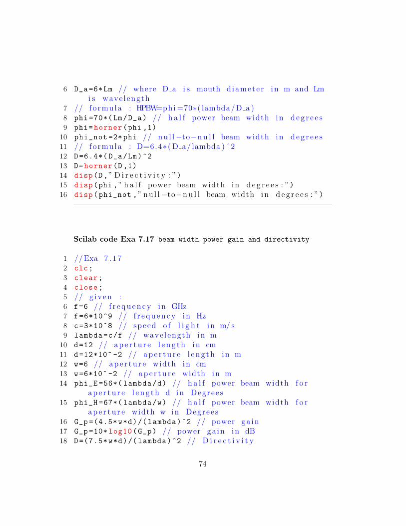
6 D_a =6*Lm // where D a i s mouth d iamete r i n m and Lmi s wave l ength

7 // fo rmu la : HPBW=phi =70∗( lambda /D a )8 phi =70*( Lm/D_a) // h a l f power beam width i n d e g r e e s9 phi=horner(phi ,1)

10 phi_not =2*phi // n u l l −to−n u l l beam width i n d e g r e e s11 // fo rmu la : D=6.4∗ ( D a/ lambda ) ˆ212 D=6.4*( D_a/Lm)^2

13 D=horner(D,1)

14 disp(D,” D i r e c t i v i t y : ”)15 disp(phi ,” h a l f power beam width i n d e g r e e s : ”)16 disp(phi_not ,” n u l l −to−n u l l beam width i n d e g r e e s : ”)

Scilab code Exa 7.17 beam width power gain and directivity

1 //Exa 7 . 1 72 clc;

3 clear;

4 close;

5 // g i v e n :6 f=6 // f r e q u e n c y i n GHz7 f=6*10^9 // f r e q u e n c y i n Hz8 c=3*10^8 // speed o f l i g h t i n m/ s9 lambda=c/f // wave l ength i n m

10 d=12 // a p e r t u r e l e n g t h i n cm11 d=12*10^ -2 // a p e r t u r e l e n g t h i n m12 w=6 // a p e r t u r e width i n cm13 w=6*10^ -2 // a p e r t u r e width i n m14 phi_E =56*( lambda/d) // h a l f power beam width f o r

a p e r t u r e l e n g t h d i n Degree s15 phi_H =67*( lambda/w) // h a l f power beam width f o r

a p e r t u r e width w i n Degree s16 G_p =(4.5*w*d)/( lambda)^2 // power ga in17 G_p =10* log10(G_p) // power ga in i n dB18 D=(7.5*w*d)/( lambda)^2 // D i r e c t i v i t y

74

19 disp(phi_E ,” h a l f power beam width f o r a p e r t u r el e n g t h d i n Degree s : ”)

20 disp(phi_H ,” h a l f power beam width f o r a p e r t u r e widthw i n Degree s : ”)

21 disp(G_p ,” power ga in i n dB : ”)22 disp(D,” D i r e c t i v i t y : ”)

Scilab code Exa 7.18 power gain of a square horn antenna

1 // Exa 7 . 1 82 clc;

3 clear;

4 close;

5 Lm=poly(0, ’Lm ’ ) // d e f i n i n g Lm as lambda6 d=8*Lm // where d i s a p e r t u r e l e n g t h and Lm i s

wave l ength7 w=8*Lm // where w i s a p e r t u r e width8 // fo rmu la : G p =(4.5∗w∗d ) / lambda ˆ29 G_p =(4.5*w*d)/Lm^2 // power ga in

10 G_p=horner(G_p ,1)

11 G_p =10* log10(G_p) // power ga in i n dB12 disp(G_p ,” power ga in i n dB : ”)

Scilab code Exa 7.19 power gain and directivity of a horn antenna

1 //Exa 7 . 1 92 clc;

3 clear;

4 close;

5 // g i v e n :6 f=6 // f r e q u e n c y i n GHz7 f=6*10^9 // f r e q u e n c y i n Hz8 c=3*10^8 // speed o f l i g h t i n m/ s

75

9 lambda=c/f // wave l ength i n m10 d=10 // a p e r t u r e l e n g t h i n cm11 d=10*10^ -2 // a p e r t u r e l e n g t h i n m12 w=5 // a p e r t u r e width i n cm13 w=5*10^ -2 // a p e r t u r e width i n m14 G_p =(4.5*w*d)/( lambda)^2 // power ga in15 G_p =10* log10(G_p) // power ga in i n dB16 D=(7.5*w*d)/( lambda)^2 // D i r e c t i v i t y17 D=10* log10(D) // d i r e c t i v i t y i n dB18 disp(G_p ,” power ga in i n dB : ”)19 disp(D,” D i r e c t i v i t y i n dB : ”)

Scilab code Exa 7.20 complementary slot impedances

1 //Exa 7 . 2 02 clc;

3 clear;

4 close;

5 // g i v e n :6 eta_0 =377 // i n t r i n s i c impedance i n ohm7 disp(”when Zd=73+%i ∗4 2 . 5 ”)8 Zd=73+%i*42.5 // d i p o l e impedance9 // fo rmu la : z s ∗ zd=( e t a 0 ) ˆ2/410 Zs=eta_0 ^2/(4* Zd) // s l o t impedance i n ohm11 disp(Zs,” complementary s l o t impedance i n ohm : ”)12

13 disp(”when Zd=67+%i∗0 ”)14 Zd=67+%i*0 // d i p o l e impedance15 // fo rmu la : z s ∗ zd=( e t a 0 ) ˆ2/416 Zs=eta_0 ^2/(4* Zd) // s l o t impedance i n ohm17 disp(Zs,” complementary s l o t impedance i n ohm : ”)18

19 disp(”when Zd=710+%i∗0 ”)20 Zd=710+%i*0 // d i p o l e impedance21 // fo rmu la : z s ∗ zd=( e t a 0 ) ˆ2/4

76

22 Zs=eta_0 ^2/(4* Zd) // s l o t impedance i n ohm23 disp(Zs,” complementary s l o t impedance i n ohm : ”)24

25


32


39

40 disp(”when Zd=50−%i∗25 ”)41 Zd=50-%i*25 // d i p o l e impedance42 // fo rmu la : z s ∗ zd=( e t a 0 ) ˆ2/443 Zs=eta_0 ^2/(4* Zd) // s l o t impedance i n ohm44 disp(Zs,” complementary s l o t impedance i n ohm : ”)45

46

47 disp(”when Zd=300+%i∗0 ”)48 Zd=300+%i*0 // d i p o l e impedance49 // fo rmu la : z s ∗ zd=( e t a 0 ) ˆ2/450 Zs=eta_0 ^2/(4* Zd) // s l o t impedance i n ohm51 disp(Zs,” complementary s l o t impedance i n ohm : ”)

77

Chapter 9

WAVE PROPAGATION

Scilab code Exa 9.1 Required transmitter power

1 //Exa 9 . 12 clc;

3 clear;

4 close;

5 // g i v e n :6 f=1.7 // f r e q u e n c y i n MHz7 f=1.7*10^6 // f r e q u e n c y i n Hz8 E=0.5 // e l e c t r i c f i e l d i n mV/m9 E=0.5*10^( -3) // e l e c t r i c f i e l d i n V/m

10 sigma =5*10^ -5 // c o n d u c t i v i t y i n mho/cm11 eta =0.5 // e f f i c i e n c y12 epsilon_r =10 // r e l a t i v e p e r m i t t i v i t y13 c=3*10^8 // speed o f l i g h t i n m/ s14 lambda=c/f // wave l ength i n m15 d=10 // d i s t a n c e i n km16 d=10*10^3 // d i s t a n c e i n m17 Df =1.8*10^12*( sigma/f) // d i s s i p a t i o n f a c t o r18 b=atand (( epsilon_r +1)/Df) // phase c o n s t a n t i n

d e g r e e s19 p=(%pi/Df)*(d/lambda)*cosd(b) // n u m er i c a l d i s t a n c e20 A=((2+0.3*p)/(2+p+0.6*p^2))-(sind(b)*(sqrt(p/2)*exp

78

((-5*p)/8))) // f a c t o r o f the ground l o s s e s21 // fo rmu la : E=(A∗E not ) /d22 // E not =300∗ s q r t (P kW) // E not i s i n mV/m23 // E not =300∗ s q r t (P kW) ∗10ˆ(−3) // E not i s i n V/m24 P_kW=(E*d*10^ -3/(A*300*10^ -3))^2 // Power i n kW and

d i s i n km25 // fo rmu la : P=Ptx∗ e t a26 Ptx=P_kW/eta // t r a n s m i t t e r power r e q u i r e d i n kW27 disp(Ptx*1000,” t r a n s m i t t e r power r e q u i r e d i n W: ”)28

29

30 // note : answer i n the book i s wrong . s c i l a b g i v e Ptx=11.48W whereas answer i n the book i s Ptx =12.6W

Scilab code Exa 9.2 field strength of the ground wave

1 //Exa 9 . 22 clc;

3 clear;

4 close;

5 // g i v e n :6 disp(” f o r f r e q u e n c y =500kHz”)7 f1 =500*10^3 // f r e q u e n c y i n Hz8 c=3*10^8 // speed o f l i g h t i n m/ s9 lambda1=c/f1 // wave l ength i n m

10 d=100 // d i s t a n c e i n km11 d=100*10^3 // d i s t a n c e i n m12 Pt=100 // t r a n s m i t t e r power i n kW13 eta =50 // e f f i c i e n c y i n p e r c e n t a g e14 eta =0.5 // e f f i c i e n c y15 P_kW=Pt*eta // r a d i a t e d power i n kW16 E_not =300*1.28* sqrt(P_kW) // f i e l d s t r e n g t h i n mV/m

without ground l o s s e s at 1km17

18 // f o r s e a water e a r t h

79

19 epsilon_r =81 // p e r m i t t i v i t y20 sigma =45*10^ -3 // c o n d u c t i v i t y i n mho/cm21 Df =1.8*10^12*( sigma/f1) // d i s s i p a t i o n f a c t o r22 b=atand(( epsilon_r +1)/Df) // phase c o n s t a n t i n

d e g r e e s23 p=(%pi/Df)*(d/lambda1)*cosd(b) // n u me r i c a l d i s t a n c e24 A=((2+0.3*p)/(2+p+0.6*p^2))-(sind(b)*(sqrt(p/2)*exp

((-5*p)/8))) // f a c t o r o f the ground l o s s e s25 E1=(A*E_not)/(d) // i n V/m26 disp(E1*1000,” e l e c t r i c f i e l d s t r e n g t h f o r s ea water

e a r t h i n mV/m when f =500kHz : ”)27

28 // f o r good s o i l29 epsilon_r =20 // p e r m i t t i v i t y30 sigma =10^ -4 // c o n d u c t i v i t y i n mho/cm31 Df =1.8*10^12*( sigma/f1) // d i s s i p a t i o n f a c t o r32 b=atand(( epsilon_r +1)/Df) // phase c o n s t a n t i n

d e g r e e s33 p=(%pi/Df)*(d/lambda1)*cosd(b) // n u m er i c a l d i s t a n c e34 A=((2+0.3*p)/(2+p+0.6*p^2))-(sind(b)*(sqrt(p/2)*exp

((-5*p)/8))) // f a c t o r o f the ground l o s s e s35 E2=(A*E_not)/(d) // i n V/m36 disp(E2*1000,” e l e c t r i c f i e l d s t r e n g t h f o r good s o i l

i n mV/m when f =500kHz : ”)37

38 // f o r poor s o i l39 epsilon_r =10 // p e r m i t t i v i t y40 sigma =0.2*10^ -4 // c o n d u c t i v i t y i n mho/cm41 Df =1.8*10^12*( sigma/f1) // d i s s i p a t i o n f a c t o r42 b=atand(( epsilon_r +1)/Df) // phase c o n s t a n t i n


((-5*p)/8))) // f a c t o r o f the ground l o s s e s45 E3=(A*E_not)/(d) // i n V/m46 disp(E3*1000,” e l e c t r i c f i e l d s t r e n g t h f o r poor s o i l


80

48 // f o r c i t i e s , i n d u s t r i a l a r e a s49 epsilon_r =5 // p e r m i t t i v i t y50 sigma =10^ -5 // c o n d u c t i v i t y i n mho/cm51 Df =1.8*10^12*( sigma/f1) // d i s s i p a t i o n f a c t o r52 b=atand(( epsilon_r +1)/Df) // phase c o n s t a n t i n

d e g r e e s53 p=(%pi/Df)*(d/lambda1)*cosd(b) // n u me r i c a l d i s t a n c e54 A=((2+0.3*p)/(2+p+0.6*p^2))-(sind(b)*(sqrt(p/2)*exp

((-5*p)/8))) // f a c t o r o f the ground l o s s e s55 E4=(A*E_not)/(d) // i n V/m56 disp(E4*1000,” e l e c t r i c f i e l d s t r e n g t h f o r c i t i e s ,

i n d u s t r i a l a r e a s i n mV/m when f =500kHz : ”)57

58 // f o r Rockey s o i l , f l a t sandy59 epsilon_r =10 // p e r m i t t i v i t y60 sigma =2*10^ -3 // c o n d u c t i v i t y i n mho/cm61 Df =1.8*10^12*( sigma/f1) // d i s s i p a t i o n f a c t o r62 b=atand(( epsilon_r +1)/Df) // phase c o n s t a n t i n


((-5*p)/8))) // f a c t o r o f the ground l o s s e s65 E5=(A*E_not)/(d) // i n V/m66 disp(E5*1000,” e l e c t r i c f i e l d s t r e n g t h f o r Rockey

s o i l , f l a t sandy i n mV/m when f =500kHz : ”)67

68 // f o r medium h i l l s , f o r e s t a t i o n69 epsilon_r =13 // p e r m i t t i v i t y70 sigma =5*10^ -5 // c o n d u c t i v i t y i n mho/cm71 Df =1.8*10^12*( sigma/f1) // d i s s i p a t i o n f a c t o r72 b=atand(( epsilon_r +1)/Df) // phase c o n s t a n t i n


((-5*p)/8))) // f a c t o r o f the ground l o s s e s75 E6=(A*E_not)/(d) // i n V/m76 disp(E6*1000,” e l e c t r i c f i e l d s t r e n g t h f o r medium

h i l l s , f o r e s t a t i o n i n mV/m when f =500kHz : ”)

81

77

78

79

80 disp(” f o r f r e q u e n c y =1500kHz”)81

82 f2=1500 // i n kHz83 f2 =1500*10^(3) // i n Hz84 lambda2=c/f2 // i n m85 // f o r s e a water e a r t h86 epsilon_r =81 // p e r m i t t i v i t y87 sigma =45*10^ -3 // c o n d u c t i v i t y i n mho/cm88 Df =1.8*10^12*( sigma/f2) // d i s s i p a t i o n f a c t o r89 b=atand(( epsilon_r +1)/Df) // phase c o n s t a n t i n


((-5*p)/8))) // f a c t o r o f the ground l o s s e s92 E1=(A*E_not)/(d) // i n V/m93 disp(E1*1000,” e l e c t r i c f i e l d s t r e n g t h f o r s ea water

e a r t h i n mV/m when f =1500kHz : ”)94

95 // f o r good s o i l96 epsilon_r =20 // p e r m i t t i v i t y97 sigma =10^ -4 // c o n d u c t i v i t y i n mho/cm98 Df =1.8*10^12*( sigma/f2) // d i s s i p a t i o n f a c t o r99 b=atand(( epsilon_r +1)/Df) // phase c o n s t a n t i n


((-5*p)/8))) // f a c t o r o f the ground l o s s e s102 E2=(A*E_not)/(d) // i n V/m103 disp(E2*1000,” e l e c t r i c f i e l d s t r e n g t h f o r good s o i l


105 // f o r poor s o i l106 epsilon_r =10 // p e r m i t t i v i t y107 sigma =0.2*10^ -4 // c o n d u c t i v i t y i n mho/cm108 Df =1.8*10^12*( sigma/f2) // d i s s i p a t i o n f a c t o r

82

109 b=atand(( epsilon_r +1)/Df) // phase c o n s t a n t i nd e g r e e s

110 p=(%pi/Df)*(d/lambda2)*cosd(b) // n u me r i c a l d i s t a n c e111 A=((2+0.3*p)/(2+p+0.6*p^2)) -(sind(b)*(sqrt(p/2)*exp

((-5*p)/8))) // f a c t o r o f the ground l o s s e s112 E3=(A*E_not)/(d) // i n V/m113 disp(E3*1000,” e l e c t r i c f i e l d s t r e n g t h f o r poor s o i l


115 // f o r c i t i e s , i n d u s t r i a l a r e a s116 epsilon_r =5 // p e r m i t t i v i t y117 sigma =10^ -5 // c o n d u c t i v i t y i n mho/cm118 Df =1.8*10^12*( sigma/f2) // d i s s i p a t i o n f a c t o r119 b=atand(( epsilon_r +1)/Df) // phase c o n s t a n t i n

d e g r e e s120 p=(%pi/Df)*(d/lambda2)*cosd(b) // n u me r i c a l d i s t a n c e121 A=((2+0.3*p)/(2+p+0.6*p^2)) -(sind(b)*(sqrt(p/2)*exp

((-5*p)/8))) // f a c t o r o f the ground l o s s e s122 E4=(A*E_not)/(d) // i n V/m123 disp(E4*1000,” e l e c t r i c f i e l d s t r e n g t h f o r c i t i e s ,

i n d u s t r i a l a r e a s i n mV/m when f =1500kHz : ”)124

125 // f o r Rockey s o i l , f l a t sandy126 epsilon_r =10 // p e r m i t t i v i t y127 sigma =2*10^ -3 // c o n d u c t i v i t y i n mho/cm128 Df =1.8*10^12*( sigma/f2) // d i s s i p a t i o n f a c t o r129 b=atand(( epsilon_r +1)/Df) // phase c o n s t a n t i n


((-5*p)/8))) // f a c t o r o f the ground l o s s e s132 E5=(A*E_not)/(d) // i n V/m133 disp(E5*1000,” e l e c t r i c f i e l d s t r e n g t h f o r Rockey

s o i l , f l a t sandy i n mV/m when f =1500kHz : ”)134

135 // f o r medium h i l l s , f o r e s t a t i o n136 epsilon_r =13 // p e r m i t t i v i t y137 sigma =5*10^ -5 // c o n d u c t i v i t y i n mho/cm

83

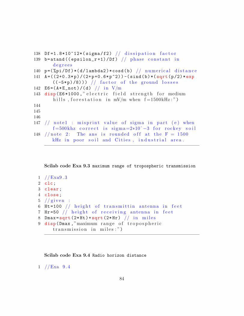
138 Df =1.8*10^12*( sigma/f2) // d i s s i p a t i o n f a c t o r139 b=atand(( epsilon_r +1)/Df) // phase c o n s t a n t i n


((-5*p)/8))) // f a c t o r o f the ground l o s s e s142 E6=(A*E_not)/(d) // i n V/m143 disp(E6*1000,” e l e c t r i c f i e l d s t r e n g t h f o r medium

h i l l s , f o r e s t a t i o n i n mV/m when f =1500kHz : ”)144

145

146

147 // note1 : m i s p r i n t v a l u e o f s igma i n pa r t ( e ) whenf =500 khz c o r r e c t i s s igma =2∗10ˆ−3 f o r r o ckey s o i l

148 // note 2 : The ans i s rounded o f f a t the F = 1500kHz i n poor s o i l and C i t i e s , i n d u s t r i a l a r ea .

Scilab code Exa 9.3 maximum range of tropospheric transmission

1 // Exa9 . 32 clc;

3 clear;

4 close;

5 // g i v e n :6 Ht=100 // h e i g h t o f t r a n s m i t t i n antenna i n f e e t7 Hr=50 // h e i g h t o f r e c e i v i n g antenna i n f e e t8 Dmax=sqrt (2*Ht)+sqrt (2*Hr) // i n m i l e s9 disp(Dmax ,”maximum range o f t r o p o s p h e r i c

t r a n s m i s s i o n i n m i l e s : ”)

Scilab code Exa 9.4 Radio horizon distance

1 //Exa 9 . 4

84

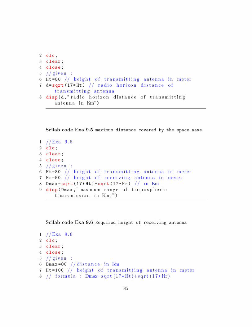
2 clc;

3 clear;

4 close;

5 // g i v e n :6 Ht=80 // h e i g h t o f t r a n s m i t t i n g antenna i n meter7 d=sqrt (17*Ht) // r a d i o h o r i z o n d i s t a n c e o f

t r a n s m i t t i n g antenna8 disp(d,” r a d i o h o r i z o n d i s t a n c e o f t r a n s m i t t i n g

antenna i n Km”)

Scilab code Exa 9.5 maximum distance covered by the space wave

1 //Exa 9 . 52 clc;

3 clear;

4 close;

5 // g i v e n :6 Ht=80 // h e i g h t o f t r a n s m i t t i n g antenna i n meter7 Hr=50 // h e i g h t o f r e c e i v i n g antenna i n meter8 Dmax=sqrt (17*Ht)+sqrt (17*Hr) // i n Km9 disp(Dmax ,”maximum range o f t r o p o s p h e r i c

t r a n s m i s s i o n i n Km: ”)

Scilab code Exa 9.6 Required height of receiving antenna

1 //Exa 9 . 62 clc;

3 clear;

4 close;

5 // g i v e n :6 Dmax =80 // d i s t a n c e i n Km7 Ht=100 // h e i g h t o f t r a n s m i t t i n g antenna i n meter8 // fo rmu la : Dmax=s q r t (17∗Ht )+s q r t (17∗Hr )

85

9 Hr=(Dmax -(sqrt (17*Ht)))^2/17 // h e i g h t o f r e c e i v i n gantenna i n m

10 disp(Hr,” h e i g h t o f r e c e i v i n g antenna i n m”)

Scilab code Exa 9.7 Radio horizon distance for transmitting and receiving antenna and maximum range

1 //Exa 9 . 72 clc;

3 clear;

4 close;

5 // g i v e n ;6 Ht=300 // h e i g h t o f antenna i n f e e t7 Hr=100 // h e i g h t o f r e c e i v i n g antenna i n f e e t8 dt=sqrt (2*Ht) // r a d i o h o r i z o n d i s t a n c e f o r a

t r a n s m i t t i n g antenna i n m i l e s9 dr=sqrt (2*Hr) // r a d i o h o r i z o n d i s t a n c e f o r a

t r a n s m i t t i n g antenna i n m i l e s10 dmax=dt+dr // maximum range o f space wave

p r o p a g a t i o n i n m i l e s11 disp(dt,” r a d i o h o r i z o n d i s t a n c e f o r a t r a n s m i t t i n g

antenna i n m i l e s : ”)12 disp(dr,” r a d i o h o r i z o n d i s t a n c e f o r a r e c e i v i n g

antenna i n m i l e s : ”)13 disp(dmax ,”maximum range o f space wave p r o p a g a t i o n

i n m i l e s : ”)

Scilab code Exa 9.8 range of the space wave

1 //Exa 9 . 82 clc;

3 clear;

4 close;

5 // g i v e n :

86

6 f=60 // i n MHz7 f=60*10^6 // i n Hertz8 c=3*10^8 // speed o f l i g h t i n m/ s9 lambda=c/f // wave l ength i n meter10 Ptx=1 // t r a n s m i t t i n g power i n k i l o watt11 ht=50 // h e i g h t o f t r a n s m i t i n g antenna i n meter12 hr=5 // h e i g h t o f r e c e i v i n g antenna i n meter13 E=80 // e l e c t r i c f i e l d i n micro V/m14 E=80*10^( -6) // e l e c t r i c f i e l d i n V/m15 E0 =3*137.6* sqrt(Ptx)*(8/5) *10^3 // f i e l d i n mV/m at

1 meter where Ptx i s i n kW16 E0 =3*137.6* sqrt(Ptx)*(8/5) *10^3*10^( -3) // f i e l d i n

V/m at 1 meter where Ptx i s i n kW17 // fo rmu la : E=(4∗( %pi ) ∗ht ∗hr ∗E0 ) /( lambda∗d ˆ2)18 d=sqrt ((4* %pi*ht*hr*E0)/( lambda*E)) // range o f

space wave i n meter19 disp(d/1000,” range o f space wave i n Km: ”)

Scilab code Exa 9.9 maximum wavelength at which propagation is possible

1 //Exa 9 . 92 clc;

3 clear;

4 close;

5 // g i v e n :6 hd=30 // h e i g h t o f duct i n m7 delta_M =30 // u n i t l e s s8 LAMBDA_max =2.5* hd*sqrt(delta_M *10^ -6) // maximum

wave l ength at which duct p r o p a g a t i o n i s p o s s i b l e9 disp(LAMBDA_max ,”maximum wave l ength at which duct

p r o p a g a t i o n i s p o s s i b l e i n m: ”)

Scilab code Exa 9.10 Electron density of the layer

87

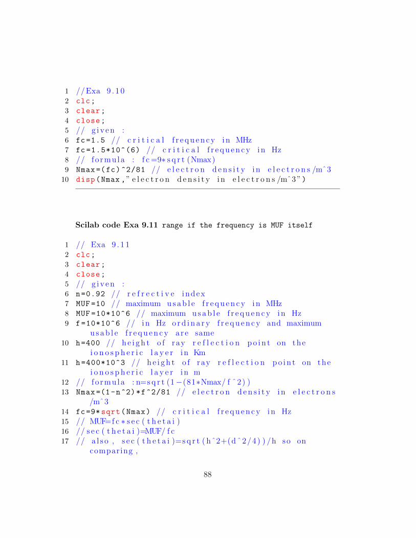
1 //Exa 9 . 1 02 clc;

3 clear;

4 close;

5 // g i v e n :6 fc=1.5 // c r i t i c a l f r e q u e n c y i n MHz7 fc =1.5*10^(6) // c r i t i c a l f r e q u e n c y i n Hz8 // fo rmu la : f c =9∗ s q r t (Nmax)9 Nmax=(fc)^2/81 // e l e c t r o n d e n s i t y i n e l e c t r o n s /mˆ310 disp(Nmax ,” e l e c t r o n d e n s i t y i n e l e c t r o n s /mˆ3 ”)

Scilab code Exa 9.11 range if the frequency is MUF itself

1 // Exa 9 . 1 12 clc;

3 clear;

4 close;

5 // g i v e n :6 n=0.92 // r e f r e c t i v e index7 MUF =10 // maximum u s a b l e f r e q u e n c y i n MHz8 MUF =10*10^6 // maximum u s a b l e f r e q u e n c y i n Hz9 f=10*10^6 // i n Hz o r d i n a r y f r e q u e n c y and maximum

u s a b l e f r e q u e n c y a r e same10 h=400 // h e i g h t o f ray r e f l e c t i o n p o i n t on the

i o n o s p h e r i c l a y e r i n Km11 h=400*10^3 // h e i g h t o f ray r e f l e c t i o n p o i n t on the

i o n o s p h e r i c l a y e r i n m12 // fo rmu la : n=s q r t (1−(81∗Nmax/ f ˆ2) )13 Nmax=(1-n^2)*f^2/81 // e l e c t r o n d e n s i t y i n e l e c t r o n s

/mˆ314 fc=9* sqrt(Nmax) // c r i t i c a l f r e q u e n c y i n Hz15 // MUF=f c ∗ s e c ( t h e t a i )16 // s e c ( t h e t a i )=MUF/ f c17 // a l s o , s e c ( t h e t a i )=s q r t ( hˆ2+(d ˆ2/4) ) /h so on

comparing ,

88

18 d=sqrt ((( MUF*h/fc)^2-h^2)*4) // range i n km19 disp(d/1000,”Range i n Km”)20

21

22 // note : answer i n the book i s 1 8 7 6 . 5 9 where as i ns c i l a b i s 1 8 7 7 . 9 4 minute d i f f e r e n c e on ly

Scilab code Exa 9.12 Relative permittivity of D E F layers

1 //Exa 9 . 1 22 clc;

3 clear;

4 close;

5 // g i v e n ;6 f=50 // i n hz7 f=50*10^3 // i n KHz8 N1=400 // e l e c t r o n d e n s i t y o f D l a y e r i n e l e c t r o n s /

cmˆ39 N2 =5*10^5 // e l e c t r o n d e n s i t y o f E l a y e r i n

e l e c t r o n s /cmˆ310 N3 =2*10^6 // e l e c t r o n d e n s i t y o f F l a y e r i n

e l e c t r o n s /cmˆ311 // fo rmu la : n=s q r t ( e p s i l o n r )=s q r t (1−(81∗N/ f ˆ2) ) //

WHERE f IS IN KhZ12 // f o r D l a y e r13 epsilon_r1 =1 -(81*N1/f^2) // r e l a t i v e p e r m i t t i v i t y o f

D l a y e r14 // f o r E l a y e r15 epsilon_r2 =1 -(81*N2/f^2) // r e l a t i v e p e r m i t t i v i t y o f

E l a y e r16 // f o r F l a y e r17 epsilon_r3 =1 -(81*N3/f^2) // r e l a t i v e p e r m i t t i v i t y o f

F l a y e r18 disp(round(epsilon_r1),” r e l a t i v e p e r m i t t i v i t y o f D

l a y e r : ”)

89

19 disp(epsilon_r2 ,” r e l a t i v e p e r m i t t i v i t y o f E l a y e r : ”)20 disp(epsilon_r3 ,” r e l a t i v e p e r m i t t i v i t y o f F l a y e r : ”)

Scilab code Exa 9.13 Angle of refraction

1 // Exa 9 . 1 32 clc;

3 clear;

4 close;

5 // g i v e n :6 f=50 // i n hz7 f=50*10^3 // i n KHz8 theta_i =30 // i n d e g r e e s9 N=400 // e l e c t r o n d e n s i t y o f D l a y e r i n e l e c t r o n s /cm

ˆ310 // fo rmu la : n=s q r t ( e p s i l o n r )=s q r t (1−(81∗N/ f ˆ2) ) //

WHERE f IS IN KhZ11 // f o r D l a y e r12 epsilon_r =1 -(81*N/f^2) // r e l a t i v e p e r m i t t i v i t y o f D

l a y e r13 n=sqrt(epsilon_r) // r e f r e c t i v e index14 // fo rmu la : n s i n ( t h e t a r )=s i n ( t h e t a i ) // s n e l l ’ s

law15 theta_r=asind(sind(theta_i/n)) // a n g l e o f

r e f r a c t i o n i n d e g r e e s16 disp(theta_r ,” a n g l e o f r e f r a c t i o n i n d e g r e e s : ”)

Scilab code Exa 9.14 critical frequency of an electromagnetic wave

1 //Exa 9 . 1 42 clc;

3 clear;

4 close;

90

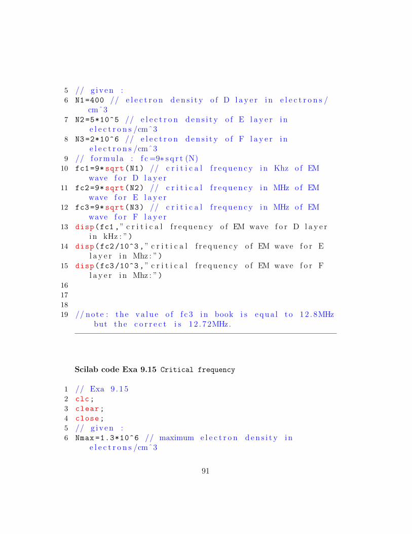
5 // g i v e n :6 N1=400 // e l e c t r o n d e n s i t y o f D l a y e r i n e l e c t r o n s /

cmˆ37 N2 =5*10^5 // e l e c t r o n d e n s i t y o f E l a y e r i n

e l e c t r o n s /cmˆ38 N3 =2*10^6 // e l e c t r o n d e n s i t y o f F l a y e r i n

e l e c t r o n s /cmˆ39 // fo rmu la : f c =9∗ s q r t (N)10 fc1 =9* sqrt(N1) // c r i t i c a l f r e q u e n c y i n Khz o f EM

wave f o r D l a y e r11 fc2 =9* sqrt(N2) // c r i t i c a l f r e q u e n c y i n MHz o f EM

wave f o r E l a y e r12 fc3 =9* sqrt(N3) // c r i t i c a l f r e q u e n c y i n MHz o f EM

wave f o r F l a y e r13 disp(fc1 ,” c r i t i c a l f r e q u e n c y o f EM wave f o r D l a y e r

i n kHz : ”)14 disp(fc2/10^3,” c r i t i c a l f r e q u e n c y o f EM wave f o r E

l a y e r i n Mhz : ”)15 disp(fc3/10^3,” c r i t i c a l f r e q u e n c y o f EM wave f o r F

l a y e r i n Mhz : ”)16

17

18

19 // note : the v a l u e o f f c 3 i n book i s e q u a l to 1 2 . 8MHzbut the c o r r e c t i s 1 2 . 7 2MHz.

Scilab code Exa 9.15 Critical frequency

1 // Exa 9 . 1 52 clc;

3 clear;

4 close;

5 // g i v e n :6 Nmax =1.3*10^6 // maximum e l e c t r o n d e n s i t y i n

e l e c t r o n s /cmˆ3

91

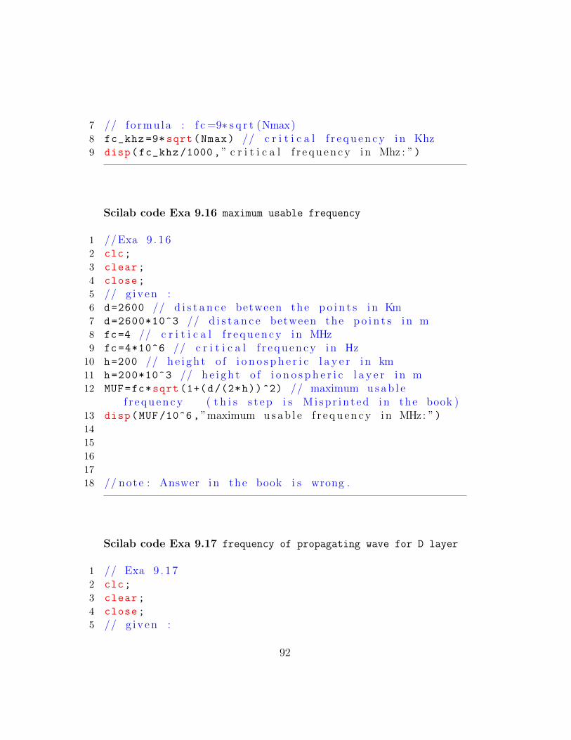
7 // fo rmu la : f c =9∗ s q r t (Nmax)8 fc_khz =9* sqrt(Nmax) // c r i t i c a l f r e q u e n c y i n Khz9 disp(fc_khz /1000 ,” c r i t i c a l f r e q u e n c y i n Mhz : ”)

Scilab code Exa 9.16 maximum usable frequency

1 //Exa 9 . 1 62 clc;

3 clear;

4 close;

5 // g i v e n :6 d=2600 // d i s t a n c e between the p o i n t s i n Km7 d=2600*10^3 // d i s t a n c e between the p o i n t s i n m8 fc=4 // c r i t i c a l f r e q u e n c y i n MHz9 fc =4*10^6 // c r i t i c a l f r e q u e n c y i n Hz

10 h=200 // h e i g h t o f i o n o s p h e r i c l a y e r i n km11 h=200*10^3 // h e i g h t o f i o n o s p h e r i c l a y e r i n m12 MUF=fc*sqrt (1+(d/(2*h))^2) // maximum u s a b l e

f r e q u e n c y ( t h i s s t e p i s M i s p r i n t e d i n the book )13 disp(MUF/10^6,”maximum u s a b l e f r e q u e n c y i n MHz: ”)14

15

16

17

18 // note : Answer i n the book i s wrong .

Scilab code Exa 9.17 frequency of propagating wave for D layer

1 // Exa 9 . 1 72 clc;

3 clear;

4 close;

5 // g i v e n :

92

6 N=400 // e l e c t r o n d e n s i t y i n e l e c t r o n s /cmˆ37 n=0.5 // r e f r e c t i v e index8 // fo rmu la : n=s q r t (1−(81∗N/ f ˆ2) )9 f=sqrt (81*N/(1-n^2)) // f r e q u e n c y i n kHz10 disp(f,” f r e q u e n c y o f p r o p a g a t i n g wave i n kHz : ”)

Scilab code Exa 9.18 Range of line of sight

1 //Exa 9 . 1 82 clc;

3 clear;

4 close;

5 // g i v e n :6 Ht=60 // h e i g h t o f t r a n s m i t t i n g antenna i n meter7 Hr=6 // h e i g h t o f r e c e i v i n g antenna i n meter8 d=sqrt (17*Ht)+sqrt (17*Hr) // i n Km9 disp(d,” range o f l i n e o f s i g h t i n Km: ”)

Scilab code Exa 9.19 Critical angle of propagation for D layer

1 //Exa 9 . 1 92 clc;

3 clear;

4 close;

5 // g i v e n :6 d=500 // d i s t a n c e between t r a n s m i t t e r and r e c e i v e r

i n km7 h=70 // h e i g h t o f D l a y e r i n km8 theta_c=asind(h/(sqrt(h^2+(d^2/4)))) // c r i t i c a l

a n g l e i n d e g r e e s9 disp(theta_c ,” c r i t i c a l a n g l e o f p r o p a g a t i o n i n

d e g r e e s : ”)10

93

11

12

13 // i t can a l s o be c a l c u l a t e d from14 theta_c=atand (2*h/d) // c r i t i c a l a n g l e i n d e g r e e s15 disp(theta_c ,” c r i t i c a l a n g l e o f p r o p a g a t i o n i n

d e g r e e s by method 2 : ”)

94

scilab textbook companion for antenna and wave propagation

Documents