1

School of Technology and Society

MA

STE

R D

EG

RE

E P

RO

JEC

T

VALUE AT RISK (VaR) METHOD: AN APPLICATION FOR SWEDISH NATIONAL PENSION FUNDS (AP1, AP2, AP3)

BY USING PARAMETRIC MODEL

Master degree project in Financial EconomicsMaster in FinanceSpring term 2007

Students:Blanka GrubjesicEda Orhun

Supervisor: Hong WuExaminer: Max Zamanian

2

TABLE OF CONTENT

Abstract

CHAPTER 1. INTRODUCTION............................................................................ 51.1 Background........................................................................................................... 51.2 Purpose.................................................................................................................. 61.3 Outline of the Thesis........................................................................................... 7

CHAPTER 2. THEORETICAL FRAMEWORK: OUTLINE OF VaR METHOD.. 82.1 Basic Characteristics of VaR ............................................................................... 82.2 VaR methods......................................................................................................102.2.1 Parametric model (Variance/Covariance approach) .............................112.2.2 Historic and Monte Carlo Simulation......................................................142.2.3 VaR tools......................................................................................................162.2.4 Backtesting VaR models ............................................................................182.3 Recent Studies about Various Applications of VaR.....................................19

CHAPTER 3. PENSION FUNDS...............................................................................223.1 Pension System ..................................................................................................223.2 Risk Factors ........................................................................................................243.3 Role and characteristics of AP funds..............................................................273.4 Application of Value at Risk in Pension Funds ............................................33

CHAPTER 4. EMPIRICAL ANALYSIS......................................................................374.1 Data......................................................................................................................374.2 Methodology.......................................................................................................384.2.1 Calculating returns and standard deviations ...........................................384.2.2 Modified duration calculations for fixed income ...................................404.2.3 Formation of correlation matrix ...............................................................414.2.4 DEAR calculations .....................................................................................42

CHAPTER 5. ANALYSIS AND DISCUSSION OF RESULTS .................................435.1 Presentation and Discussion of Results .........................................................435.2 Limitations of Empirical Study and Results ..................................................45

CHAPTER 6. CONCLUSION AND RECOMMENDATIONS................................476.1 Conclusion ..........................................................................................................476.2 Recommendations for Further Research .......................................................48

7. REFERENCES.........................................................................................................49

8. APPENDIX ……... ...................................................................................................53

3

FIGURES, TABLES AND GRAPHS

Figure 1: Back-testing VaR ..............................................................................................................19Figure 2: Factors that influence balance between pension contributions and disbursements...............................................................................................................................................................25Figure 3: New pension system ........................................................................................................28Figure 4: Possible scenarios of the net contribution during period from 2007 to 2057 ........29

Table 1: Correlation Matrix..............................................................................................................42Table 2: DEAR Estimations at 95% Confidence Level ..............................................................44Table 3: DEAR Estimations at 99% Confidence Level ..............................................................44Table 4: Other risk measures and return of funds for 2005 .......................................................45

Graph 1: Percentage of realized total return after expenses for AP1, AP2 and AP3 funds for 2006 ......................................................................................................................................................31Graph 2: Composition of portfolio for AP funds for 2006 ........................................................32

4

VALUE AT RISK (VaR) METHOD: AN APPLICATION FOR SWEDISH NATIONAL PENSION FUNDS (AP1, AP2, AP3) BY

USING PARAMETRIC MODEL

ABSTRACT

Value at Risk (VaR) approach has been extensively used by investment and commercial banks since its development by JP Morgan in 1990s. As time passes, it has become interesting to investigate whether VaR could be used also by other financial intermediaries like pension funds and insurance companies. The aim of this paper is to outline Value at Risk (VaR) methodology by giving more emphasis on parametric approach which is used for empirical section and to investigate the applicability and usefulness of VaR in pension funds. After providing theoretical framework for VaR approach, the paper continues with pension fund systems in general and especially highlights AP funds of Swedish National pension fund system by trying to show why VaR could be an invaluable risk management tool for these funds together with other traditional risk measures used. Based on this given theoretical frame, a practical application of VaR –parametric or covariance/variance method- is executed on 50 biggest investments in the fixed income and equity portfolios of three selected Swedish national pension funds – AP1, AP2 and AP3. Results of one day VaR (DEAR) estimations on 30/12/2005 for each fund have been presented and it is aimed to show the additional information that could be obtained by using VaR and which is not always apparent from other risk measures employed by funds. According to the two traditional risk measures which are active risk and Sharpe ratio; AP2 and AP3 lie in the same risk level for 2005 which can create a contradiction by considering their different returns. On the other hand, obtained DEAR estimates show their different risk exposures even with the 50 biggest investments employed. The results give a matching relationship between return of funds and DEAR estimates meaning that; the fund with the highest return has the highest DEAR value and the fund with the lowest return has the lowest DEAR value; which is consistent with the main rule- “higher risk, higher return”. Thus, we can conclude that VaR could be applied additionally to get a better picture about real risk exposures and also to get valuable information on expected possible loss together with other traditional risk measures used.

Key words: Value at Risk, DEAR, Pension funds, Risk management, Swedish pension plan, AP1, AP2, AP3

5

CHAPTER 1. INTRODUCTION

1.1 Background

In today’s volatile and complex market environment, financial auditorium have witnessed to the cases where the lack of good assessment and control of risk had led to thecatastrophic consequences. Especially, the historical evolution of financial markets accompanied with an adoption of the flexible exchange rate regimes, sudden oil price shocks and high volatility in interest rates and stock markets encouraged strong development of Financial Risk Management in the last thirty years. Moreover, fast growing globalization and risk connected with the emerging markets pointed out the necessity of improvement and usage of the more advanced risk management tools. (Jorion, 2001, p.4) This new area deals with various financial risks - market, credit, liquidity, operational and legal risks; in order to find solutions for better trade off between return and these risk factors.

At that point, as one of the most powerful tools of financial risk management Value at Risk (VaR) Method or literally called RiskMetrics Model has been developed in 1990s by the financial services company, J.P. Morgan with the initial intention of measuring the extent of exposure to market risks. VaR can be defined simply that it tries to answer the question of “What is the most likely value that I can expect to lose if things go wrong?” (Introduction to Value at Risk (VaR)-Part 1, Investopedia). VaR model has become so popular within financial industry due to its simplicity that it summarizes the “down-side” or “worst-case” risk of the company with one simple number. Moreover, instead of focusing on particular instruments, VaR can capture most of the risk factors financial institutions confront and offer useful insights on risk which can serve as a decision criterion in determination of the capital cushion. By taking into consideration this fact, commercial banks are let by regulators to use their own internal models to assess their market risk instead of the standardized model which was used before 1998 when BIS (Bank for International Settlements) updated this decision. However, it should not be forgotten that the internal VaR model should be set up very carefully in order to prevent future failures.

After this evolution of VaR, pension funds; which are also at the heart of financial industry together with commercial banks and other financial institutions; began to take attention for the applicability of this model. Risk Management within pension funds has begun to be addressed heavily when this millennium started. Before this date, particularly during 1980s and 1990s the equities that funds are invested in were providing stable and higher returns that were adequately enough to cover retirement benefits of the beneficiaries. This positive situation would not have required for pension fund managers and regulators to investigate alternative risk management methods. However, conditions began to change

6

severely by the turn of the millennium due to financial turmoil in the Asian financial markets that affected several countries in the world and dot.com business failures. Thus, Financial Risk Management and various tools of this area like VaR started to be very attractive for stakeholders of pension funds including policy makers and regulators in order to identify and address their risk exposures. While the size of pension funds’ total assets makes them a vital participant of the financial markets, on the other hand, their social role in providing stable and safe retirement system attracts a great deal of interest from the regulators and publicity. (Development in Pension Fund Risk Management in Selected OECD and Asian Countries, n.d., p.2)

In this regard, the question of VaR implementation is very challenging one, keeping in mind that pension funds should provide retirement benefits and therefore higher returns in the long horizon. There are a lot of risk factors that influence pension funds’ assets and liabilities. On the liabilities side, they are affected by demographic impacts for instance decrease in the number of individuals working today relative to the number of retired persons, which is one of the main reasons of inefficiency of the pay-as-you-go system. Mortality rates and fiscal policy that do not allow further tax increase for funding retirement payments are further liability side risk factors. In addition to all these, biometric risk factors that stem from actuarial assumptions like the longevity, death and disability in life are another important risk aspect for pension fund management. On the asset side, however, pension funds confront different types of risk due to various and global instruments they invest in. Those asset side risks are even more emphasized because of the necessity to invest in more risky assets to obtain returns that can bear the burden of growing disbursement requirements. Mainly, asset side risk is composed of two headings that are “asset-liability mismatching” (where assets on hand are not enough to meet benefits when they are due) and “return related risks” (where insufficient or very volatile income is generated over time which is not sufficient to cover liabilities). Thus, VaR comes into the stage as a valuable risk management tool due to its ability to combine different types of risks while assessing the total portfolio of the company. (Development in Pension Fund Risk Management in Selected OECD and Asian Countries, n.d.) Despite the fact that VaR could be used as a powerful tool for measuring the risk, there exist some vital decisions to be taken related to some specific characteristics of VaR methods, definitions of fundamental parameters in evaluation and pension funds’ specificities.

1.2 Purpose

As it is outlined above, the applicability of VaR models for pension funds is present as an interesting research area due to the challenges that should be identified and solved. With this in mind, this research aims to provide an analysis and understanding of VaR techniques by trying to answer the question “What makes this method such useful and why it could be used also by pension funds as a back-up instrument of other risk measures like Sharpe and Information ratios?”.

7

Although the main focus of this paper is on VaR, it aims to focus on its practical application on real world issues. Due to this, three AP funds (AP1, AP2 and AP3) of Swedish National pension system are taken as the subjects of VaR analysis. After providing the necessary theoretical background on VaR, pension funds in general, Swedish National pension system and selected AP funds, empirical VaR analysis will be executed. Accordingly,the empirical analysis part tends to provide funds’ comparison by utilizing their major risk exposures in order to estimate one day VaR (DEAR) values on 30/12/2005 through the usage of parametric approach of VaR. With this aim, for each selected fund, 20 biggest Swedish stocks, 20 biggest foreign stocks and 10 biggest fixed-income investments (bonds) has been identified which has been utilized to make normal stock and fixed income investment DEAR estimations that will reflect the possible “worst-case scenario” risk exposures of funds. Foreign exchange risk exposure on foreign stocks and bonds would not have been taken into consideration in the purpose of this study. Additionally, it will be discussed why VaR approach could be used additionally and together with other risk measures in order to get better insight about the risk exposure.

1.3 Outline of the Thesis

This paper is organized into five main parts after the introduction chapter. Chapter 2 provides an introduction into Value at Risk methodology; with examination of the historic factors and environment that influenced the evolution of advanced risk management tools. Further, this unit gives an essential theoretical frame for understanding VaR concept and application of it. Here basic methods and calculation techniques are discussed and accompanied with detailed description of parameters needed for VaR estimation. Moreover, comparative analysis of advantages and shortcomings of each method is provided with examples. Finally, this chapters turns to examination of alternative VaR methods and toolsand also it presents recent studies and research about the various usage areas of VaR.

Next, Chapter 3 presents general information about pension systems and the risk factors that they confront. It puts more emphasis on AP funds of Swedish National pension system by explaining their characteristics and the reform process, three of which are selected as the subjects of empirical part. This section concludes with the discussion why application of VaR is supportive and could provide additional useful information for pension funds meaning that traditional risk measures should be backed up with VaR in order to get better insight.

Afterward, Chapter 4 of the paper tackles an empirical analysis and application of VaR on three Swedish national buffer funds – First, Second and Third AP funds or shorter AP1, AP2 and AP3. Parametric approach is applied on their biggest part of equity and bond portfolios for the purpose of getting insight into their risk exposures. Description of methods used and sequences analyzed, leads to Chapter 5 where results are presented and

8

evaluated with comparison of each fund’s one-day Value at Risk estimation and conclusions about their trade off between risk factors and return are included.

After discussing the obtained results and usefulness of VaR in Chapter 5, the general conclusion part together with some recommendations for further research constitutes the last part-Chapter 6- of the thesis.

CHAPTER 2. THEORETICAL FRAMEWORK: OUTLINE OF VaR METHOD

2.1 Basic Characteristics of VaR

The period of 1970s is characterized with high volatility of financial markets driven by the oil price shocks and sharp stock prices and interest rates movements. Furthermore, beginning from this period we can witness a rapid evolution of derivative markets through occurrence of broad variety and complexity of those instruments. Although, their first intention was hedging, they were also used for speculation purposes, quite often accompanied with unawareness or ignorance of the risks involved. Due to these circumstances, some of the well known and publicized financial disasters took place, such as Barings, Orange County, Daiwa, Procter & Gamble and many others. All these events inevitably led to the increased consciousness about risk monitoring and highlighted the importance and the necessity of developing new methods to deal with uncertainty. That is to say, derivatives which are developed for hedging the market risk in fact began to be a problem instead of a solution that created incentives for companies to find better risk management methods. (Jorion, 2001)

In this way, in 1994 J.P.Morgan’s management also wanted to know better its exposure to the risk and assessment of possible losses across all its firms and branches operating in different countries, at the end of the day. The result was development of RiskMetrics model, which provided information of maximum dollar amount of expected losses over the chosen confidence level and under the normal circumstances. Because of its simplicity, as well as definition of risk in new probabilistic way and its quantification, Value at Risk became widely accepted foremost in the investment area. Furthermore, since then simple RiskMetrics model has evolved into more complex methods with the main aim to capture the different types of risks and apply this method in varying situations. Because of its advantages over the classic risk-management tools, corporations, pension funds, insurance corporations and other institutions started to explore potentiality of VaR.

Basically, we can define VaR as quantile (or percentile) based risk measure, which provides the maximum expected loss under some probability level. Here the word “maximum expected loss” should be emphasized because VaR does not provide a number

9

for loss value that will be realized for sure at the end of the time period. For example, if the one day VaR equals to 500.000 SEK at 95% confidence level, it means that the financial institution can expect with 95% certainty, loss should not exceed 500.000 SEK during one day. However, the maximum possible loss can be much higher. From previous example it is obvious that we have to define variables such as confidence level, time period that VaR refers to and standard deviation (volatility) of the variable that reflects the adverse deviations from the mean. Therefore, parameters needed for estimation can be grouped in the following way:

Characteristics of the portfolio:

o Overall portfolio value marked to market – represents the value of all the items in the balance sheet of financial institution if they would be bought or sold at present market prices or in other words, their present value

o Volatility of portfolio – in order to get an insight how worse possible losses can get, we need to measure total deviations of each return Xi ; which could be stock returns or any other variable; that enables us to measure the volatility of the asset or portfolio; from its mean values μ, i.e. we have to define variance and standard deviation:

22 )(1

1

iXN

, where 2 (Watsham, Parramore,

2006)

Time horizon – definition of holding period is extremely important for correct interpretation of VaR. First of all, because volatility grows with square root of time, increase of time will produce higher VaR. According to Jorion (2001, p.116), time horizon should be chosen depending on the application of VaR. Therefore, if it is used to get general insight over different types of risk, the choice is more of subjective nature and the only request is consistency. However, if VaR is used as an indicator for possible losses, then the liquidity criterion should be used, i.e. the time in which portfolio can be sold out and the risk positions can be corrected.

Additionally, in the case when computation of VaR is used for estimation of capital needed for coverage of possible losses, time horizon should be defined not only by the liquidity criterion, but also by the risk aversion level of the company as well as the cost of a possible loss exceeding VaR. Eventually, selection of the long horizon will decrease the number of independent observations that are used to understand how good our VaR estimation really is. Hence, this is an important factor that will have impact on the application of VaR in pension funds. As it will be observed later, for the empirical part of this study time period will be selected as one day for each AP fund in order to estimate

10

their one day VaR values or Daily earnings at risk values (DEARs). One day has been used as the time period because as pension funds’ investment periods are much longer than just five or ten days, it has been thought that calculating one day VaR values would be more reasonable for comparison purposes.

Confidence level– It can be defined as a statistical value that measures the degree of certainty about a forecast. In the context of VaR, it can be interpreted as the probability that true value of loss will fall within an estimated interval. Hence, in given example VaR of 500.000 SEK at 95% confidence level means that 95% of time expected loss should not extend outside of the given value limit. Like in the case of the time horizon, larger confidence level will increase VaR number and decision criteria for selecting confidence level also depends on the characteristics of the financial institution. For instance, those that exhibit higher degree of risk aversion are likely to choose higher confidence level since it will end up with a more conservative or higher VaR value so that managers would be more prepared to worse outcomes. In addition, choice of the appropriate confidence level also depends on considerations regarding back testing. Back testing is amethod of checking out estimated VaR losses by comparing them with losses that really occurred during the underlying period. As it is mentioned before, 95% confidence level means that 95% of the time, loss should not go beyond the estimated VaR value. Obviously, in the case of 99% confidence level, a manager will have to wait for longer time to review the success of VaR estimation because a higher confidence level decreases the expected number of observations in thetail or so-called the possible results for extreme scenarios. Therefore, having back testing purposes in mind, 95% level is highly recommended (Jorion, 2001). On the other hand, because of the concern that financial institutions can intentionallytry to underestimate their risk level in order to minimize the capital requirementfor the undertaken risk by choosing lower confidence levels, regulators such as Bank for International Settlements (BIS), proposed higher confidence level that is99% rather then 95% as well as a minimum time period of 10 days (Saunders, 2006, p.280). In the case of this study, DEAR values for each AP fund will be estimated both at 95% and 99% confidence levels in order to have a complete picture.

2.2 VaR methods

As a result of different kind of assumptions in VaR calculations, such as presuming the type of distribution, three main models have evolved:

Parametric model (Variance/Covariance approach) Historic simulation Monte Carlo simulation

11

2.2.1 Parametric model (Variance/Covariance approach)

The main assumption of parametric model is that returns of assets in the portfolio and so total portfolio returns are normally distributed. This model can be summarized by a simple formula:

VVDEAR

where DEAR is Daily Earnings at Risk or the VaR measure for one day, V represents the market value of the asset (the present value of the asset if it is wanted to be sold/bought in today’s market conditions), volatility of risk factors (this is the standard deviation ofreturns or values of the underlying asset that can be bonds, stocks, FX investments…), is critical value that equals to +/- 1.65 for 95% confidence level or +/- 2.33 for 99% confidence level and μ is the expected value, i.e. mean value of the asset. However, it is very common in the Variance/Covariance approach to consider the expected change in a market variable –μ here- over the time period as zero. This is usually a reasonable assumption bytaking into consideration that the expected change–μ- in a market variable is much smaller than the standard deviation-σ- of the variable. When this assumption has been realized and μhas been taken as zero, the formula would return simply to VDEAR (Jorion, 2003 & Hull, 2006). Furthermore, if we are interested in VaR value for more than one day, we will

have to multiply the DEAR value with square root of time; N (Saunders, Cornett, 2006 &Parametric VaR Estimation-Risk Metrics Group).

In order to better understand this main formula of parametric VaR approach which also constitutes the empirical part of this study, examples for various investment assets like bonds, stocks and FX investments; which also make up the main investment categories of pension funds in general; have been provided in the following section. Stocks and bond investments of these examples are the main assets that will be utilized in the empirical part later for three Swedish AP funds.

-Example 1 for Stock:

Assume that, we have a stock which is traded on the market whose current market value is 5000 SEK. Other than knowing the market value of the shares, the potential risk in this equity position should also be discovered. As the Capital Asset Pricing Model (CAPM) asserts, there exist two types of risks in an individual stock (і) position which are systematic and unsystematic risks that constitute the total risk together as follows (Saunders, Cornett, 2006):

icRiskUnsystematRiskSystematicTotalRisk ; or

12

)()()( 2222eitmtiit

While the unsystematic risk is specific to the firm in question, the systematic risk or market risk derives from holding the market portfolio. Each stock reacts to the market movements with a coefficient which is present in the formula as βi. That is to say, the volatility of the stock- it - depends on the market volatility- mt -, reaction or co-movement of this stock to

this market volatility- i -and to the risk which is totally independent from the market but

specific to the firm- eit -. It is believed that in a very well diversified portfolio, unsystematic risk disappears due to the fact that one firm’s risk can be compensated by another’s meaning that while one performing badly, the other can perform well. Thus, in a well diversified portfolio only systematic risk remains. It is even possible to say that when the investor distributes his money evenly in every stock of the market and so replicates a market portfolio, this portfolio constructed will move same with the market itself that means βi

would be taken as one. In this situation, the risk would be simplified to the volatility of the market- 2

mt . However, it should not be forgotten that this last assumption can be extremely strong to be agreed on in many cases (Bodie, Kane, Marcus, 2006 & CAPM-Risk Glossary, 1996).

For this example, if we know that the volatility- mt - of the daily returns on the stock market index was 1 percent, then by accepting all assumptions above the VaR value for 10 days could be calculated as follows by using MV of the stock, value for the confidence level from the normal table and the volatility of the market index:

SEKVaR 887.2601001.065.15000

This calculated number represents at least 260.887 SEK stands to be lost if adverse stock market returns become realized in the following 10 days. If DEAR value would be calculated meaning that square root of 10 would be removed from the calculation, then the result would reflect the potential loss in the next day.

It should be also noted that the β of the stock or the portfolio could be inserted into the formula as a multiplication in order to get a better insight, if it is not for sure that the portfolio at hand is not fully successful at replicating the market index.

-Example 2 for Bond:

For the bond example, suppose we have a bond for which we want to estimate VaR. Our first step would be to determine its market value, in this case we assume one year zero coupon bond of 1.000 SEK nominal value and that interest rates on similar instruments are 3%. Thus, market value of that bond is 970.87 SEK which can be found by using the general present value formula. Next step is to gauge an extent which will point out how much theprice of the bond will fall in response to a small increase in the interest rates, or in other words we have to find duration and modified duration (in the case of a zero coupon bond,

13

duration equals to maturity and if it is divided by 1+R we will get modified duration i.e. 0.971). Assuming the normal distribution, estimation of standard deviation is quite easy –suppose in this case it equals to 0.035. Additionally, we will take level of confidence is 95% and time horizon 10 days as given. In this particular case VaR is determined in the following way:

SEKVaR 16.17210035.065.1971.087.970 This number could be interpreted in the same way as in the case of previous stock example.

-Example 3 for Foreign Exchange (FX) Investment:

As a last example, calculation of VaR value for an FX investment will be provided subsequently:

Assume that we have 2000 € position invested in spot euros. The first step in calculating VaR should be converting this value to the main currency unit in which all VaR calculations are executed that is Swedish Crones in our case. This conversion can be carried out by using the EUR/SEK spot exchange rate of that day that is 9.2867 for this example.

Thus, SEK Equivalent Value of Position SEK4.185732867.92000

We know that in order to have the VaR value, we need a volatility measure which would be the volatility of FX rate for this example. The volatility or standard deviation of FX rate can be obtained by looking back to the daily changes in FX rate EUR/SEK over some past years which has been given as 0.0041 for this illustration. In this way, VaR for this FX position for a ten days period at 95 % confidence level will result like that (Saunders, Cornett, 2006):

SEKVaR 337.397100041.065.14.18573

Furthermore, these kinds of calculations similar to ones in these examples can be broadened for whole portfolio of the financial institution with certain adjustments to the type of the instrument we are dealing with. For instance, valuation for derivatives which is not illustrated with an example, their deltas should take place in the formula. However, we should keep in mind that VaR for whole portfolio is not simple sum of all individual VaR components. In that case we would disregard a diversification effect and positive influence of less than perfect correlation on reducing the risk. Consequently, VaR of two assets can be represented by following formula (Value at Risk-RiskMetrics, n.d.):

212,12

22

1 ***2 assetassetassetassetassetasset VaRVaRVaRVaRVaR

14

Hence, it can be inferred that parametric model is relatively simple for application and it enables straightforward aggregation of portfolio positions by computing correlations between them. However, the main drawback of this method is the normal distribution postulation.

On the other hand, it is obvious that a financial institution that is dealing with many different financial assets daily would not just invest in two assets. Thus, the formula above could be adjusted to infinite number of assets as below:

ijj

N

i iji

N

ii DEARDEARDEARDEAR

11

2 2

Alternatively, the DEAR of a portfolio can be calculated by finding the aggregate standard deviation of return on the portfolio and multiplying it with the value of the confidence level. Suppose we have a portfolio P that consists n assets with an amount wi

being invested in asset i. Return on asset i for one day is defined as δxi. So, the return on portfolio P will be equal to:

i

n

ii xwP

1

As a next step, we need to find the mean and standard deviation of P . It is assumed that the expected value of each δxi is zero which implies the mean of P is also zero. For calculating standard deviation of P , it would require the daily volatility-

ix -of the return

on i th asset and coefficient of correlation- ij - between return on asset i- ix - and asset j-

jx . Then the variance of P , which will be denoted by 2P , can be written as:

jiji

n

i ijiji

n

iiP www

1

2

1

22 2

Hence, the VaR value for the portfolio can be obtained by multiplying standard deviation of the portfolio- P - with the confidence interval value and square root of number

of days- N (Hull, 2006). Both of these alternative two ways would provide the same VaR value at the end.

2.2.2 Historic and Monte Carlo Simulation

Second most common and simple way of finding VaR value is historic or back simulation. Unlike the parametric or RiskMetrics approach, it does not set any kind of

15

assumption about the type of distribution in advance which provides a big advantage especially for some assets like options which exhibit non-normal return distribution due to their unlimited upside or downside returns (losses). Moreover, historical approach requires sufficient historical time series and it simply use them to simulate future risk positions. Application of this method can be summarized in a few steps. First of all, we have to define and evaluate our risky positions. Similar to parametric model, sensitivity of each position to adverse market movements needs to be computed. Additionally, the total loss or gain of the position will be given by the price sensitivity times actual price changes. The repetition of this step for every single day of our historical data set is required. Finally, after retrieving all past returns we sort them in order from worst to best and cut off 5% or 1% of the worst losses, according to selected confidence level. If we take our previous example with FX investment,after writing down our FX position in SEK, we need to calculate Delta of position or in other words, the measure which shows how much the SEK value of FX position will change if the FX rate depreciates by one percent against Euro for this example. Then, by looking to the realized FX rate changes over the past days- say 500 days here- and using the delta value calculated, the risk exposure or the loss value should be calculated for each day. These losses should be arranged in ascending order and at the 95 % confidence level or 5 % worst case scenario, 25th (500 days x 5 %) observation from the bottom will represent our VaR estimate. This procedure can be updated every day, but it requires a main assumption that past returns can provide good estimation of future and it makes us to confront the problem of relevance of data far away from the present moment. For example, if we are analyzing high-tech stocks and we are using time series that spans over the last 20 years, it is questionable if dotcom bubble of the late 90’s is relevant for the future predictions of price movements. One of the suggested solutions is assigning higher weights to the more recent data (Saunders & Cornett, 2006, p.272).

However, as the response to the problems of these two methods which are mainly assuming normal distribution for the parametric model and past reflect future well enough for the historic simulation model, an alternative, but also technically more complicated method in the form of Monte Carlo simulation has been developed. By using a predefined distribution, Monte Carlo simulates large number of possible returns that should reflect their recent historical occurrence. Therefore, this method is similar to back simulation method, in the way that it uses historical data to retrieve possible outcomes, but on the other hand their predictions are not just simple replication of past because additional random observations are created by the simulation that are highly probable to occur in recent historic time periods. Its relationship with parametric approach can be drawn in the way that both approaches demand presumption of the distribution, although in the case of parametric model this assumption is limited just with the normal distribution, which is not the case with Monte Carlo simulation (Saunders & Cornett, 2006).

Finally, selection of the right method will depend on advantages and limitations of each approach and characteristics of particular portfolio and institution. Obviously, the main advantage of parametric method is in its simplicity and straightforwardness. However, in spite of its simplicity, this model requires calculation of the variance-covariance matrix,

16

which in case of large portfolios can be a daunting task. Furthermore, as a main drawback, the assumption of normal distribution should be emphasized. A great deal of asset returns, especially stocks and derivatives exhibit fat tail and skewed distributions, with extreme returns that result in inability of using this method without some major modifications. Moreover, at this point some assumptions concerning time scaling should be mentioned as well. As stated above, volatility increases with time or more precisely with square root of time. This holds only if price or return movements exhibit homoscedasticity, i.e. if they have finite variance. Besides, mean reversion as well as presence of trend will overestimate or underestimate volatility, respectively. (Value at Risk-Riskmetrics, n.d.)

The main advantage of historic or back simulation model over parametric one is in the fact that it does not require normal distribution. Regarding simplicity, it can be inferred that historic approach does not demand calculation of correlation matrices, but on the other hand measuring risk for every past observation may also involve considerable time for its development. Furthermore, earlier mentioned requirement for significant amount of time series and difficulties in defining which historic data are relevant, are additional shortcomings of this method.

Consequently, it can be inferred that Monte Carlo simulation is superior to other methods, because it is designed to overcome some of the mentioned problems. However, it demands software and substantial time for setting up the model as well as for obtaining the results.

By considering all these characteristics of three main methods of VaR, in this study parametric model will be employed due to its simplicity so that it would be possible to be understood by many people. In real life situations, this model has been also very popularized by managers because it is easy to understand and much more simple to construct. Although it is possible to claim that Monte Carlo Simulation method could give better results, it will not be used here due to the high amount of time required to construct the model and get results with the large portfolio at hand for three Swedish National pension funds and also due to a sophisticated computer program needed.

2.2.3 VaR tools

Other than these three main approaches of VaR, different tools and methods has been developed over time for active risk management. Three most important VaR tools would be explained briefly here:

Marginal VaR Incremental VaR Component VaR

17

First of the three, the aim of calculating Marginal VaR is to determine the effect of altering positions on the portfolio risk. It is simply calculated by finding the change in the portfolio VaR that result from shouldering an additional dollar exposure in a given component which is a security in the case of a general portfolio. Because it is a marginal measure, it is calculated by taking the partial derivative of initial VaR estimate with respect to the component weight. It is a very useful dimension since it shows the sole effect of one asset on the aggregate portfolio value which is not possible to be extracted from the general VaR estimation. By knowing the individual marginal VaRs of different assets that exist in the portfolio, managers would take better decisions regarding additional investments on those assets (Jayaraman, Denton, 2004, p.3).

The second VaR tool; incremental VaR; also provides useful information for risk managers. It finds the additional VaR value that stems from a new trading position. To be more clear, it could be represented by the formula; Incremental VaR = VaR P+A – VaR P where VaR P represents the VaR value of the initial position and VaR P*A represents the VaR valueof the new position that includes an additional amount of A dollars exposed newly to the risk factors. It could be very time-consuming to obtain incremental VaR value especially for large portfolios because it requires the calculation of VaR value twice for different trading positions. On the other hand, it is possible to find the trading position which will minimize the portfolio risk that is so called “best hedge position” through this tool. Additionally, it should not be mixed with marginal VaR which gives a unit value but differently incremental VaR can be used for larger changes in the position (Jorion, 2001, p.154).

The last variant of VaR tools; component VaR; is used to decompose the portfolio risk into its components. Thus, it shows the proportion of each component in the aggregate portfolio risk meaning that sum of individual component VaRs gives the total VaR value. It is calculated by the help of Marginal VaR that is a measure of unit risk for one component. So, component VaR can be represented by the formula, CVaRi= MVaRi x wi where wi

represents the weight of the component i in the portfolio. As it can be understood, CVaR also tells us how the portfolio VaR will change if this specific component is taken away. The concept of CVaR in fact is not limited only to calculation of portfolio VaRs. Instead, it can be even utilized to understand the risk allocation within business units or departments of a whole enterprise.

In the context of our study, these VaR tools are not planned to be employed because the aim here is to estimate the aggregate portfolio VaR value for the selected Swedish national pension funds and compare their risk level by examining the obtained VaR estimation values. However, extension of this study could be segregating the total portfolio VaR value of the pension funds into its components that would be individual assets invested in or the main financial asset blocks (stocks, bonds, FX investments…) by using component VaR tool.

18

2.2.4 Backtesting VaR models

After building their VaR models and obtaining VaR values through these models, financial institutions should verify whether the VaR model constructed gives accurate resultsboth for their own sake and for fulfilling regulatory requirements. This verification process is called back-testing and it should be performed at least on a quarterly basis. The easiest way to back-test would be to plot realized profits & losses (P&Ls) against estimated VaR values and to see to which extent they match each other. As an example, suppose that we are calculating 1-day 95 % VaR values. While we are back-testing, we will find out how often the loss in a day exceeds the 1-day 95 % calculated VaR value for that day. If this happens on average 5 % of the total days, then we can feel ourselves as confident to say that our VaR model works well enough (Hull, 2006). The excess deviations of P&Ls over VaR values can sometimes occur with a higher percentage value, say in this case 6 % or 7 %, which could be attributed simply to bad luck. On the other hand, if these deviations result as such a great number, say 20 % which would be compared with 5 %, then the validity of the VaR model need to be questioned (Jorion, 2001). And, in some cases it can be necessary to begin building the VaR model from the scratch. Additionally, while observing deviations from estimated VaR values, it should be also ensured that those deviations are dispersed evenly over time period. It is not our desire to observe that all deviations are clustered at one specific time for the reliability of our model (Backtesting VaR-Risk Metrics, n.d.).

Such a plot that is used for back-testing purposes has been provided below in Figure 1 in order to give better insight for the main method of Back-testing.

19

Figure 1: Back-testing VaR

Source: Risk Metrics Group

2.3 Recent Studies about Various Applications of VaR

After presenting VaR approach and its different methods in the previous parts, this section will review the previous studies and research that have used VaR for different purposes and in different business sectors. However, it should not be forgotten that this paper mainly investigates the application of VaR in pension funds and it will continue by focusing on pension funds and VaR application on those and then it will present the empirical application on AP funds of Swedish national pension system.

As it has been many times stressed, value at risk is widely used in the investment and commercial banks. Therefore, in different reports of those banks under the section that concerns risk evaluation, VaR estimation can be found together with the description of the selected methods, time horizon and confidence level. For instance, in the risk report of Deutsche Bank (p. 183, 2002) it is stated that for both – internal and external purposes, VaR at 99% confidence level is used. Furthermore, while for internal use one-day VaR is calculated, for Bank of International Settlements ten days VaR is reported. Prevailing method

20

that is used is Monte Carlo simulation which is combined with parametric approach for some portfolios.

In addition to such reports made by practitioners, a lot of scientific research can be found as well in the banking field. Berkowitz and O’Brien (2001) analyze profits and losses and present VaR estimations of the 6 large US commercial banks in their study about accuracy of the VaR models in commercial banks. As it is shown in their survey, VaR for analyzed commercial banks varies in the range of 1.72% up to 5.62%. Reported VaR numbers are estimated at 99% confidence level and for one day horizon. This study brought out few important observations. First of all, according to the observed sample it is shown that 99% confidence level overestimates the risk. While this can have positive effect on keeping capital reserves at a higher level in the case of adverse market movements, on the other side it has been seen that VaR is not providing an accurate estimation of the real risk. Second important observation of this study is that although violations of VaR are rare, when they occur their magnitude is very high. This implies that volatility is clustering. Therefore, authors used ARMA and GARCH model on modeling the volatility of profits and losses and their evaluation showed that more accurate estimation can be obtained by using these models. Hence, the conclusion of the study is that although overstepping of VaR limits is below the permitted level of 1%, commercial banks should use more advanced VaR models in order to deal with volatility clustering by using GARCH models, which will provide, a better insight for their real risk.

There are also some studies that explore the applicabilty of VaR within pension funds and insurance companies which have much longer investment horizons compared to investment and commercial banks. One study about the application of VaR for pension funds's asset side risk; which is also the focus of this paper; is made by Gupta, Stubbs and Thambiah (2000). The objective of that study is to calculate VaR in 200 largest US corporate defined-benefit plans. The survey reports annual VaR estimations for 1998 and extrapolations for 1999. Furthermore, study analyzes obtained results by taking into consideration each fund’s sector, asset size, funding status and proportion of the portfolio invested in equity.

The survey shows that annual VaR for those funds varies within range of 9.5% up to 28%. In addition, from observation of those funds, some important conclusions can be drawn. First, value at risk is increasing function of the proportion of the assets invested in equity. Secondly, although it might be expected that under-funded pension funds would take higher risks, this is not the case. Further, degree of the risk aversion is in the reverse relation with the asset size and it is closely connected with the risk aversion in certain sectors. Finally, another important inference of this study is that in the case of the analyzed large US corporate defined-benefit funds of this study, connection between estimated VaR and

21

realized return is not found very clearly. In other words for those funds, it means that funds with higher return do not inevitably have higher VaR and vice versa.

One other study by Ahlgrim (1999) about VaR and insurance companies shows that instead of employing the whole portfolio of the company, VaR could be applied for single products of insurance companies like the whole life insurance policy which is the subject of this study. This study combines actuarial risk and VaR in one place by using Monte Carlo simulation for estimating VaR of whole life insurance policy. In order to ease the application due to the actuarial risk involved, the paper assumes a known mortality rate.

Other than these main applications of VaR for these various financial sectors, VaR can be applied for many other purposes. For instance, VaR can be calculated for stock markets and stock indices. One of such studies by Varma (1999) applies various empirical tests with different underlying models in the VaR framework for NSE-50 (Nifty) Index of Indian stock market. He uses GARCH-GED (Generalised Auto-Regressive Conditional Heteroscedasticity with Generalised Error Distribution residuals) and alternatively EWMA models to estimate time-varying volatility and finds out that GARCH-GED model performs better than EWMA model at all risk levels. Another similar study that is executed for another stock market is done by Sahin (2002). In this study, Sahin (2002) estimates VaR values for ISE (Istanbul Stock Exchange) 100 index and also for a portfolio which is composed of 5 randomly chosen stocks from the index. He estimates VaR values by using three different methods of VaR approach that are variance-covariance, historical simulation and boot-strapped simulation methods. He finds out that VaR of variance-covariance method gives lower results than that of other methods. He attributes this due to the fact that variance-covariance method assumes normal distribution of returns although the returns are not all the time normally distributed.

Another hot issue about the usage of VaR approach is that it could be also used by central banks in order to predict solvency problems and financial crises. This idea is firstly developed by Blejer and Schumacher (1998) where they prescribe how to find the net value of central bank portfolio which will be utilized for VaR estimations. After explaining how to find the net value of central bank’s portfolio, they continue by explaining how VaR should be used in the concept of central bank’s assets and liabilities. By following and extending the theory developed by Blejer and Schumacher (1998), Nocetti (2006) creates an operational model to calculate central bank’s VaR and applies this model by using data from Argentina crisis of 2001. He also compares predictive performance of VaR measure with other well-known indicators of financial crisis.

As it can be understood, VaR has many different usage opportunities with various purposes. This section tried to give a brief review about recent research and developments about VaR’s different usage areas before beginning with our main focus. The next chapter will continue with pension funds and VaR application on those which is the main focus. The paper will then continue with the empirical section.

22

This chapter (2) of the thesis tried to outline the most important concepts about VaR methods, its tools and recent studies about various VaR applications for different purposes in order to give a complete picture. However, not all these concepts are relevant for the practical application that will take place in the empirical part. Mainly, parametric model (covariance/variance method) will constitute the empirical part where DEAR estimations will be calculated for the composed portfolios of each AP fund.

CHAPTER 3. PENSION FUNDS

Pension funds constitute one of the most important segments of the financial markets, exceeding majority of the other institutional investors with size of their assets. Only in Sweden pension funds disposed with assets under management equaling to 14.5 percent of the GDP in 2006 (OECD, 2006, p.2). However, in recent decades it became evident that the pension funds tend to be more and more under-funded leading to the reforms of pension systems that took place in many countries - Italy, France, Austria, Germany, Great Britain, Sweden, Chile and many more. Although in some of the countries, reforms were inevitably connected with significant cuts in retirement benefits, Swedish government searched for less painful methods in finding the way to ensure financial stability in the long run.

This section aims to provide general overview of the pension funds and basic terms connected with them. Furthermore, it gives brief description of the situation in Sweden and about reforms that occurred in 1990s. Furthermore, it explains the role of the AP funds in Swedish pension system. Theoretical framework given in this section tends to emphasize importance of the risk management and especially application of VaR for pension funds. Consequently, discussion is upgraded by putting focus on VaR regarding specificities of the pension funds business and its comparison to the other widely used risk methods.

3.1 Pension System

Pension funds can be defined as financial intermediaries that collect funds from the working population and manage them in the way to provide retirement benefits. They pursue an important social role in smoothing the level of income and consumption by taking into consideration the wages earned during the working period of each individual. Hence, the management of collected inflows, their investment, planning the future disbursements and dealing with risks involved, attract a lot of attention of the financial economists, politicians and general public.

In general, pension funds can be categorized as the private pension funds and public pension funds. Obviously, the public pension funds are under the administration of the

23

government. Because of their role in society, in many countries vast part of the pension system is comprised of the public funds. However, there are also private funds managed by other participants in financial markets like insurance companies and investment banks. In addition, private funds can be originated by companies and funded by contributions from employers as well as employees. While public funds constitute the first pillar of the pension system, private funds usually constitute the second pillar of the pension system, meaning that they often manage smaller portion of the pension contributions set aside from income and that they are supplementary to the public funds. In most of the cases individuals are allowed to decide in which private fund they will pay in their contributions, whereas they cannot select public fund.

Two main ways at which pension funds work can be distinguished as– funded system and pay-as-you-go system. In the funded system, funds invest their assets with the purpose to save for the future cash disbursements. Most of the private funds function in this way, even in some countries for instance USA, they are obligated by the regulations to be a funded system (CBO, 2004, p.1). On the contrary, pay-as-you-go approach represents such a system in which contributions received from currently working population are used for payments to present retirees. The majority of the public funds work according to this principal. As it will be shown later, the problem that occurs with the pay-as-you-go system is that today’s pension payments are conditioned by the current contributions which are dependent on the various factors such as unemployment rate, birth and immigration rate, business cycles and so on. Some of these risk factors are not so easily predictable and they complicate themaintenance of a safe and stabile pension system.

There exist also two main ways to determine the distribution of future pensions that are defined benefit and defined contribution formula. Under the defined benefit plan, the individual is guaranteed to obtain certain pension. Retirement benefits are determined according to the working time and income. Formulas used in calculation of pensions under the defined benefit plan can be categorized in the three main groups (Saunders, Cornett; 2001, p.528): flat benefit formula (provides same benefit for every year of the employment), career average formula (pension is based on the average income during the entire working period) and final pay formula (retirement is based on the income received during the end of the individual’s working period). Although defined benefit plan tends to smooth income during individual’s life time and to minimize discrepancy between wage and pension received, there are some serious drawbacks that should be considered. The main shortfall is that most of these plans do not encourage people to work longer and some methods of the retirement distributions can lead to the inequality among different groups of the population.

Unlike the defined benefit plan, defined contribution formula does not provide a guarantee concerning future retirement benefits. While only the lower limit for socially endangered population is guaranteed, for the rest of the individuals pension will depend on their contributions as well as the return that pension fund has gained over the time. In the context of the defined contribution system, the concept of the notional accounts should be mentioned as well. Notional accounts are imaginary accounts where contributed funds from

24

each individual as well as the proportion of the belonging return are recorded. These accounts are used upon retirement for establishment of the pension benefits. Previous pension plan in Sweden was “defined benefit pay-as-you-go system” and because of its imperfections it was reformed in 1990s. System that is running now can be categorized as “notional defined contribution” system and as it will be discussed later, it is organized as partially pay-as-you-go and partially funded system (Scherman, 1999, p.55).

3.2 Risk Factors

The main pension funds' risk factors can be divided into two groups – risk factors that affect the assets side and those that affect the liabilities side of their balance sheet. This paper underlines the assets side risk with special focus on market risk, interest rate risk, and equity risk by employing those risk factors for VaR estimation. Nevertheless, because of the specificity of pension funds it is also important to observe risk that will influence pension funds’ liabilities.

From assets’ side, in order to obtain the rate of return that will cover required pension disbursements, fund management will undertake certain investment decisions allocating funds into different instruments. Inevitably, those choices are connected with risk meaning that changes in prices will lead to decline in net asset value and total returns. Moreover, it is not that just volatility of returns will have impact on value of bonds, stocks, derivatives and other instruments held by pension funds, but also credit or default risk, country or sovereign risk, operational risk, liquidity risk, insolvency risk and other risk factors. Therefore, an appropriate allocation between securities and instruments with different risk-return performances is a crucial decision for every fund manager (Mina, 2005, p.3).

Among number of factors affecting pension funds liabilities, demographic factors are frequently mentioned as a cause of current pension plan problems. Under the term of demographic factors, it is actually meant that people live longer and number of persons working and contributing to pension system is decreasing compared to the number of retired individuals. For example in case of Sweden this ratio dropped over time from 5 in the 1950s to less than 4 and it is expected to fall to 3 (Normann, Mitchell, 2000, p.3). This is often referred as the main reason why pay-as-you-go system cannot provide sufficient funds for retirement payments anymore.

In addition, salaries and growth of earnings among different groups of population will determine cash inflows and outflows of pension funds. The total level of the salaries in the economy and thus the level of contributions to pension funds are depended on the rate of employment, immigration rate, population growth and economic growth. More specifically, earlier retirement and hence higher pay-outs for pension funds can be in connection with certain sectors and occupations. For instance, it is more likely that highly

25

paid managers will get retired earlier (Blake, 2001, p.193). Therefore, different distributionsof earnings in economy will influence the timing of retirement and cash inflows for pension funds.

Moreover, various economic and political factors can influence pension funds’ liabilities. For example, instead of encouraging people to work longer, some pension plans do not make crucial distinction between pension benefits according to the working life of individuals which leads to situation where people prefer to get retired earlier. Besides, system with heavy concentration of taxes can also discourage people to work longer and earn more, resulting as higher pressure on funds’ liabilities and lower cash inflows. Furthermore, other impacts such as inflation have impact on the liabilities as well as allocation of funds by managers.

In short, risk factors that are connected with liabilities side of the pension funds can be divided into two groups – those that affect pension contributions and those that affect pension benefits. Figure 2 summarizes mentioned risks and shows factors that affect AP funds’ buffer capital.

Figure 2: Factors that influence balance between pension contributions and disbursements

Source: www.ap3.se

After dealing with pension funds’ two-sided (asset and liability) risks in general, it is worth here to concentrate on the individual risks which are elements of these two main risk groups and can be measured and controlled by VaR approach. As it is formerly mentioned, on their asset side pension funds mainly confront investment and market risk which arises from their investments in various financial instruments by using the pension benefits that they obtain from their members. Market risk is closely related with investment risk considering that market risk arises from active trading or holding investments rather for short-term (Saunders, Cornett, 2006). This investment risk and strongly related market risk are also comprised of different type of risks according to the specific financial instrument that pension funds are invested in. It takes the form of interest rate risk for fixed income assets, equity risk for stock investments and foreign exchange risk for investments denominated in foreign currencies (Price, 2005 & Moloney, 2006). It has been shown in the previous chapter with examples how VaR method can be used to measure the possible risk

26

occurring from these three kinds of investments. It is important to determine the variable that affects the value of the specific investment and to measure the volatility of this variable in order to estimate the VaR value. As it can be understood from the examples of three specific investment types in Chapter 2, the variable affecting the value of the investment changes for every type of investment. In the case of option investments the variable would be delta of the position or in the case of linear derivatives like forward contracts; it would be the composition of changes in the values of spot and forward positions regarding the forward contract (Jorion, 2001). As it could be understood, it is possible to capture the asset side risks of pension funds by carefully defining the appropriate VaR model. However, there could exist other types of risks on the asset side like credit, country (sovereign) or liquidity risks which are not possible to be appraised by usual VaR. There are other works that develop special models to measure those risks mentioned like CreditMetrics which is again developed by JP Morgan that uses a different version of VaR methodology (Saunders, Cornett, 2006).

When it comes to the liability side risks, it even gets more complicated to use VaR methods to control and measure the confronted risk at this side. As it is mentioned, liability -side risks are mainly derived from ‘biometric’ factors. (Development in Pension Fund Risk Management in Selected OECD and Asian Countries, n.d.) As mentioned above, they are related with demographic factors like population growth, immigration rate and especially the most important one is the longevity risk which means people expected to live much longer and so pension funds would have to pay annuity payments for much longer time to their pensioners (Ewijk, Ven, 2003). This kind of risk is dealt with by employing actuarial science and its assumptions. And, it is quite difficult to combine the knowledge of actuarial science and VaR method in order to be able to control the liability side risk. However, there are some studies that try to combine these two areas for the pension funds and insurance companies that face the longevity risk. In one of these studies by Ahlgrim (1999), he tries to calculate VaR value for whole life product of an insurance company by following the actuarial model for a whole life insurance policy developed by Bowers, et. al. (1986). The VaR value depends on the probability that the insured person would live to a specific age and also depends on his mortality rate. Mortality rate is assumed to be known to ease the application (Ahlgrim, 1999). This study is specific to insurance companies but the logic of using actuarial science for the longevity risk and combining it with the VaR methods would be also same for pension funds. As it can be understood, it could be possible to apply VaR for the liability side risks of pension funds but it is much more complicated and still has a long way for new studies and developments.

27

3.3 Role and characteristics of AP funds

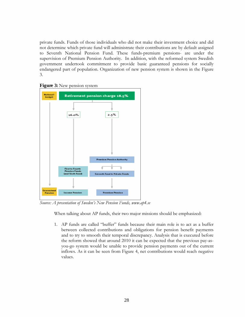
Faced with serious demographic, social and economic pressures, in 1990s it became obvious that old Swedish pension plan is not capable of providing safe and stabile retirement benefits. Old pension plan was designed as entirely pay-as-you-go system functioning as intergenerational solidarity scheme in which present working people bear the burden of pension payments for current retirees. Several factors had major impact on the inefficiency of this system. Primarily, previously mentioned longevity related with the rise in the retired population compared to the working one, is usually determined as one of the most important reasons for reform of old scheme. Previous pension plan was created as a flat-rate system indexed by prices instead of wages. Therefore, insensitivity to economic growth, led to absurd situation that when economy was strong, relationship between earnings and pension benefits decreased (Sundén, 2000, p. 1). Furthermore, system was privileged for individuals with shorter working life and higher income on expense of those working longer and earning less. This was due to the fact that pension disbursements were based on the 15 highest earning years over the working period, which creates unfair pension redistribution among different income classes and so it led to higher pensions for those with higher income oscillations compared to those with smoother income over the working period (Sundén, 2000, p. 2). Moreover, high taxes resulted as a discouragement to work longer and formed the consequence of stronger pressure on lower contributions which created the pension system insolvency (Normann, Mitchell; 2000, p.3). Besides, as taxes already reached theirceilings, their further enlargement in order to provide liquidity for future pension payments was impossible.

In 1991 it became evident that the old Swedish pension system cannot achieve its main goals – financial stability and fairness (Sundén, 2000, p. 2). At that time, a working group started to explore possibilities in order to find the most suitable solution for reforming the old system. Because of political debate, it was not until 1994 that Swedish Parliament finally accepted the proposal. The main purpose of the reform was to transfer it from entirely pay-as-you-go scheme to individual accounts and partial privatization. Essentially, the partial privatization means that previous 18.5% of taxes set apart for retirement disbursements were divided into two parts – 16 percent dedicated to finance current needs for pension withdrawals and 2.5 percent that are extracted into individual accounts and invested into different funds according to preferences of each individual. Those 16 percent is sharedwithin Swedish buffer funds “AP fonderna” – the First, Second, Third and Fourth National Pension Funds or abbreviated AP1, AP2, AP3 and AP4. The Sixth National Pension Fund (AP6) is also a buffer fund, but acts under different investment rules. These buffer (AP) funds were in existence since 1960 but they got reorganized and reestablished as a result of the reform. Following the reform, AP funds have got more competitive character. Furthermore, Swedish working people have had a wide range of -over 645- funds to choose for investment of 2.5 percent of the total wealth assigned for retirement (Palme, Sundén, Söderlind, 2004, p.2). These funds are called premium pensions and are administrated by

28

private funds. Funds of those individuals who did not make their investment choice and did not determine which private fund will administrate their contributions are by default assigned to Seventh National Pension Fund. These funds-premium pensions- are under the supervision of Premium Pension Authority. In addition, with the reformed system Swedish government undertook commitment to provide basic guaranteed pensions for socially endangered part of population. Organization of new pension system is shown in the Figure 3.

Figure 3: New pension system

Source: A presentation of Sweden’s New Pension Funds, www.ap4.se

When talking about AP funds, their two major missions should be emphasized:

1. AP funds are called “buffer” funds because their main role is to act as a buffer between collected contributions and obligations for pension benefit payments and to try to smooth their temporal discrepancy. Analysis that is executed before the reform showed that around 2010 it can be expected that the previous pay-as-you-go system would be unable to provide pension payments out of the current inflows. As it can be seen from Figure 4, net contributions would reach negative values.

29

Figure 4: Possible scenarios of the net contribution during period from 2007 to 2057

Source: Första AP-Fonden Annual Report 2006, www.ap1.se

Evidently, even under the most optimistic scenario, the old system would encounter problems very soon. Since the reform, AP funds sought to invest the inherited capital from the old system as efficient as possible in order to obtain the required rate of return that could solve the problem. Although up until now they seem to have been successful and if they continue like this they would prevent the negative net contributions, it is still early to assert that the future of the system is fully guaranteed.

2. The second mission of AP funds is to generate return that will provide long-term stability and accumulate certain reserves (Palmer, 2001, p.13). When the new pension system was introduced, buffer funds inherited capital of SEK 536 billion that was equally divided among funds (AP3 Annual Report, 2006, p.7). From 2001 until now, AP funds invested that capital with main goal to achieve considerable rate of return for the future pension needs. According to funds’ survey, rate of return that would provide financial stability of the system is estimated to be between 5.1 and 6.1 percent (Första AP Fonden, 2006, p.14). At the same time, AP funds are required to maintain level of their risk exposure as low as possible (Weaver, 2002, p.20). Because of the high volatility of the financial market, that return is not an easy goal to achieve and thus VaR can be used as a very valuable tool to manage risk while reaching the required return targets. However, in the case that mission can not be accomplished, so called balancing mechanism will be activated. Basically, that means that pension benefits will be readjusted until system stability is achieved again. Obviously, lower

30

retiree’s income would have negative social consequences. Nevertheless, current estimations suggest that so far this goal is achieved and AP funds will be able to maintain the system stability in upcoming years without cutting the pension benefits (AP3 Annual Report, 2006, p.5).

Although reform of pension plan was starting point in ensuring safety and stability of retirement system, it became evident that without major transformation of investment rules and regulations it will be impossible to provide the adequate return for future pension benefits. Low rates of return on safe instruments like government bonds were insufficient to provide long term stability of the benefit payments. Moreover, analysis conducted by AP1 fund showed that in the case that whole fund’s assets would be invested in fixed income securities, the fund would have such a low return that it would be underperformed and be unable to meet its obligations (Första AP Fonden, 2006, p.16). Inevitably, increased awareness of that risk-return issue led to the introduction of new investment rules that permitted less restrictive allocation of funds regarding allowed instruments, markets and risk exposures. New investment rules introduced in 2001 lowered proportion of assets that should be invested into bonds to 30% and at the same time increased permitted investments into equity up to 70% and tolerable currency risk exposure up to 40%.

Enforcement of new investment rules allowed a higher degree of flexibility in allocation decisions of pension funds. Even a quick glance at their balance sheet will reveal significant investments to emerging markets, foreign countries, exposures to foreign exchange and so on. Even more, an idea of further revisions and liberalization of investment rules is often brought up recently by some chief executives of buffer funds (Nordic Region Pensions & Investment News, March 2007, p.28). Therefore, departure from safer investments and shift to those instruments that will provide higher returns are also connected with much higher risk level at the same time. In such circumstances, importance of efficient risk methods, especially VaR become underlined. In addition to some traditional risk methods, VaR can provide valuable information on how much fund can expect to lose from certain investments and enable the fund management setting certain limits on acceptable level of loss.

Analyzing Swedish pension system one might ask why there are five AP funds instead of just one. Obviously, it is diversification effect on risk of the whole system that will enhance probability of its stability. Even though one fund might not fulfill its mission, distribution of the resources among more independent pension funds makes it less possible that all of them will under-perform. The differences among funds may be seen in the allocation of their assets in the various instruments and markets, different degree of reliance on external or internal management and so on. Furthermore, a competitive environment has been developed among these funds in order to make them more eager in outperforming other funds. For instance, AP1 fund established a special system of rewarding employees for surpassing performance of other funds (Weaver, 2002, p.23). Because nobody wants to end up “last in the row” and because of their search for different investment solutions, these

31

funds have different allocation structure as it will be briefly analyzed in following section(Weaver, 2002, p.25).

Independence of AP funds in their investment decisions results in their different performance and rates of return. From this point, only AP1, AP2 and AP3 funds are going to be observed, since they are in focus of our empirical analysis.

Graph 1: Percentage of realized total return after expenses for AP1, AP2 and AP3 funds for 2006

Return on total portfolio, after commision costs and operating expences, %

0,002,004,006,008,00

10,0012,0014,0016,0018,0020,00

2006 2005 2004

AP1AP2AP3

Source: Annual Reports for 2006 for AP1, AP2 and AP3, www.ap1.se, www.ap2.se, www.ap3.se.

As it can be seen from Graph 1, all three funds were almost equal with their returns in 2004. However, during 2005 and especially during 2006, AP2 outperformed other funds, gaining considerably higher return. Those distinctions can be explained by different investment decisions and allocation of funds over diverse proportions of various instruments and markets, which can be observed from Graph 2. Although AP funds grouped instruments in somewhat different classes (for instance, some classes are distinguished according to if they are hedged or not), still graphs provide quite good insight in the way that how funds designed allocation of their resources. Apparently, major contrast can be perceived among stakes invested in Swedish equity and foreign stocks. While AP1 and AP3 held 12% of their portfolios invested in Swedish stocks, AP2 invested considerable higher portion that is 20%. On the other hand AP2 had lower investments in foreign equities (hedged and non-hedged foreign equities total of 35%), comparing to AP1 and AP3 who had around 40%. Other differences can also be observed among portions invested in fixed income in which AP1 having the biggest allocation. As well as, there are distribution differences among different types of bonds for instance percentages invested in index-linked bonds and so on. Generally, by analyzing portfolio of these funds, it can be inferred that the most significant parts of assets is invested in foreign equities, fixed income and Swedish equities. Other instruments like emerging markets’ equities, private funds’ investments, real estate and alternative investments constitute a smaller part of the overall portfolio. As it will be seen later, these dominant asset classes will be used in the empirical analysis to better represent the general risk exposure of funds.

32

Graph 2: Composition of portfolio for AP funds for 2006

A P1 Strategic Portf olio f or 2006

12%

40%

5%10%

3%8%

22%

Swedish equities

Non-Swedish equities

Emerging markets' equities

Nominal Swedish f ixedincome

Nominal non-Swedish f ixedincome

Index-linked bonds

Alternativ e inv estments

AP2 Strategic Portf olio f or 2006

20%

29%6%5%

3% 1%

36%

Swedish equities

Foreign equities hedged

Foreign equities non-hedged

Emerging markets' equities

Fixed income

Real estate

Priv ate equity f unds

AP3 Strategic Portf olio f or 2006

12,0%

39,5%

3,0%6,1%

3,1%8,5%

23,4%

4,4%

Swedish equities

Non-Swedish equities

Emerging markets' equities

Nominal Swedish f ixedincomeNominal non-Swedish f ixedincomeSwedish index-linked bonds

Non-Swedish index-linkedbondsReal estate

Source: Annual Reports for 2006 for AP1, AP2 and AP3, www.ap1.se, www.ap2.se, www.ap3.se.

Additionally, to get the insight in size of those asset classes, it is worth to mention that the market value of total assets was around 200 billions SEK for each fund or more precisely, on 31st of December 2006 it equaled to SEK 207.1 billions for AP1 and SEK 216.8 and 212.2 billions for AP2 and AP3 respectively.

Finally, from everything presented about AP funds so far, it can be inferred that there are at least three important reasons why VaR should be used. First, because of their main

33

goal to provide long-term financial stability, AP funds tend to maximize their return at the lowest possible risk. By using VaR methodology, AP funds’ management will get insight in daily risk exposure. Second, the new investment rules enabled investments in the areas connected with higher return and therefore higher risk. VaR should be used for setting limits for tolerable risk exposures and bearable losses that will not jeopardize achievement of funds’ goals. Finally, because of competitive character of AP funds and their different investment decisions, VaR can be used as a tool for performance evaluation of the risk-return relation. Those funds with higher returns may simply be the ones which have undertaken higher risk without acceptable risk control.

3.4 Application of Value at Risk in Pension Funds

From its development in 1990s, Value at Risk was more designed for banks,

especially investment banks with large trading portfolios, short investment horizons and positions that turn over even during one day. Moreover, focus of the further VaR improvements was on the risk connected with banks’ business, not on longevity, unemployment or immigration rates. Nevertheless, during the time pension funds as well as other institutional investors found their interest in application of this method. However, because of the specificities of the pension funds, there are some factors to consider in the implementation of the VaR model.

First of all, unlike banks where certain regulatory framework for VaR is given by Bank for International Settlement (BIS) and Basel Accords, there are no regulatory agency providing guidelines for pension funds. Basically, this means that decisions about time horizon for VaR and confidence level depend on the judgment of the risk manager. One of the proposals was Risk Standards for Institutional Investment Managers and Institutional Investors by Capital Market Risk Advisors (Risk Standards Working Group, 1996), trying to provide general standards in implementation not only for VaR, but for other risk methods as well.

Secondly, definition of the time factor used in VaR calculations should reflect the holding period of the portfolio. Unlike the investment banks, investment horizons for pension funds are much longer, reflecting long term nature of their liabilities. As risk estimated with VaR is the function of the square root of the time, the problem that occurs is that long holding horizon might increase our estimation significantly. The question is how much it can overestimate the risk exposure. Apparently, for investment horizons of few years, deviation from the actual risk can be quite big. Moreover, correlations and volatilities estimated using daily changes, might give flawed results when using them for long horizons. This paper attempts to avoid this problem of time definition by simply using one day VaR estimation, DEAR.

34

Moreover, VaR is a method that quite successfully combines risks over various instruments in the investment banks. However, since a lot of the risk connected with pension funds are caused by the liabilities’ side risk factors that are previously mentioned, they create another difficulty in application of VaR, since they are difficult to measure. Although, there are actuarial methods that can deal with longevity risk, contributions into pension funds also depend on the factors such as unemployment rate, birth rate, immigration rate which are hard to estimate.

However, there is no doubt that VaR is a valuable tool for the pension funds as well. Pension funds’ portfolio can be divided into two parts – long term and short term portfolio. Here distinction between these portfolios is not on the maturity of the instruments that are held in them, it is rather the purpose of each portfolio. Thereby, long term portfolio or also called “policy portfolio” is long term in the sense that it is intended to ensure long period fund’s capability to meet its obligation for retirement disbursements and gain satisfying return relative to the strategic benchmark (Simons, 2001, p.2). On the other hand, short term portfolio’s purpose is to provide an additional return and thus to surpass and support performance of the policy portfolio. Here it is called short term in the sense that its investment decisions are more tactical compared to long-term strategic nature of the policy portfolio. Moreover, its positions are more frequently updated compared to long term portfolio.

In constructing the appropriate VaR model, it should be taken into account that the main measurement of the pension funds’ performance is the return relative to strategic benchmark rather than the only return itself (Simons, 2001, p.2). Essentially, strategic benchmark is an estimated portfolio that represents such a combination of various instruments over different markets and risk factors that will provide the best possible fulfillment of return requirements. To each of these asset classes associated index is awarded and the overall performance of fund is measured by comparison of its return with return on the benchmark.

When we are talking about risk methods which interpret risk and return in the correlation with strategic benchmark, there are three methods that should be mentioned because of their wide application in pension funds – tracking error, information ratio and Sharpe ratio. While these methods provide valuable information to management, they have some shortfalls as well and because of that VaR should be used as an additional method in the risk assessment.

Tracking error is a measure of the active risk calculated as the standard deviation of the portfolio return from its benchmark:

)(/1 ERERTerrorTracking t

where ERt represents excess return of the whole portfolio over the strategic benchmark in period t, while ER equals average excess return over the strategic benchmark (Simons, 2001,

35

p.5). It is also called the measure of the active risk, because it gauges departure from the index-like or passive investment strategy. Usually, tracking error is used to measure historical deviation of the return over the benchmark.

Further, Sharpe ratio represents excess of realized return relative to the volatility or the standard deviation of the portfolio (Sharpe, 1994, p.1), where the excess of the return is measured as an additional return over the risk free rate:

PfP rrratioSharpe /)(

where rP represents total portfolio return over some chosen period, rf the risk free rate and σP

standard deviation of the whole portfolio (Bodie, Kane, Marcus; 2003, p.814).

The last measure usually represented in pension funds’ annual reports is information ratio. Information ratio is similar to the Sharpe ratio and it measures excess of realized return over the return on the benchmark or in other words the alpha of the portfolio relative to the tracking error (Pomerantz, 2005, p.4):

errorTrackingrrrationInformatio BP /)(

where rB represents return on the benchmark.

Although, there is no doubt that these ratios are useful measures of risk adjusted performance, comparing to VaR we can show at least five major shortcomings. First, usually these methods measure historic performance deviations of portfolio, while VaR uses market value of the current portfolio. If the structure of portfolio had varied significantly over the time, traditional measures can produce flawed results. Second, Sharpe ratio uses risk-free rate to obtain comparison over performance of the different instruments, while VaR uses specific indicators of risk such as duration and beta. Third, neither one of the mentioned traditional methods uses duration for bonds nor beta for stocks, delta for options nor some other sensitivity indicator specific for certain instrument, making it really hard to combine different risk factors with one measure. Fourth, it is possible for tracking error measure to be quite low while the fund seriously underperformed in reality compared to the benchmark. (Simons, 2001, p.6) Assuming normal distribution of the returns relative to the strategic benchmark, there is one sixth of chance that the actual return will underperform more than tracking error. (Kemp, Cumberworth, Gardner, Griffiths and Sandford, 2000, p.10) Finally, the most important drawback is that traditional methods give an equal treatment to upside and downside risk.

Therefore, in comparison to the traditional methods there are at least four advantages of the application of VaR in the pension funds:

1. Value at risk is the risk measure that is explicitly focused on the downside risk giving straightforward information about expected losses.

2. Traditional methods mostly assume normal distribution and in the presence of the skewness and fat tails, they can give flawed results. But this problem could be

36

overcome by using VaR in the form of historical or Monte Carlo simulation that would provide more accurate estimations than traditional methods in the case of non-normal distribution.

3. Expressed in the terms of the probable losses, VaR is more intuitive and reliable measure, leaving fewer opportunities for the wrong interpretations. In the case of the funds which continuously “beat” the benchmark, traditional methods can lead to the flawed conclusion that they did not undertake risk at all (Kemp, Cumberworth, Gardner, Griffiths and Sandford, 2000, p.18).

4. While traditional methods are commonly used as backward based methods, VaR attempts to predict future losses and thus have a valuable practical usage.

It is important to emphasize that VaR is not a risk method beyond any criticism. As it is previously mentioned, each of the VaR methods has its own strengths and weaknesses that should be considered prior to the implementation. According to some surveys, parametric approach is the most frequently used VaR method in the pension funds (Simons, 2001, p.2). The main shortfall of this approach is in the fact that if the returns are not normally distributed, VaR estimation will give us flawed results by underestimating the risk in turmoil’s moments. These problems are caused by correlation estimations, which can be misleading because most of the instruments show low correlation in normal circumstances, but in the case of crisis they exhibit much higher correlation (Simons, 2001, p.10). Problems with estimation of correlation and also variances will get some attention later in this paper by mentioning some alternative econometric models to be used for estimations instead.

It can be inferred that despite the difficulties in usage of traditional methods, it is not suggested that they should be abandoned and replaced by VaR; moreover they can give some precious information about fund performance. As it is suggest by Kemp, Cumberworth, Gardner, Griffiths and Sandford (2000), fund management should be aware of the type of the information that each of the methods will provide - traditional methods will mostly provide information about risk of underperformance compared to the strategic benchmark or compared to the other funds, while with VaR information about risk will be given in the term of the expected capital loss (Kemp, Cumberworth, Gardner, Griffiths and Sandford, 2000, p.26).

Because of the different information that each of the method provides together with their advantages and weaknesses, it is important to be aware of the fact that replacement of the one method by another is not recommended. Rather it can be inferred that to get a deeper insight in return-risk relation, the risk analysis should be extended with VaR. It will be also emphasized in the empirical part that enhancing commonly used risk measures by applying VaR at the same time could give better and more reliable information on risk-return relationship.

37

CHAPTER 4. EMPIRICAL ANALYSIS

4.1 Data

As it has been already indicated, biggest 20 Swedish stocks, 20 foreign stocks and biggest 10 bond investments, which constitute the main investment categories of AP funds and thus give a good picture of their risk exposures, have been selected for DEAR estimation. Various data has been utilized in order to be able to calculate DEAR values for each 40 stocks and 10 bonds selected for each AP fund and finally to calculate the final portfolio DEAR that consists these selected bonds and stocks for each fund. Data sets used are mainly obtained from three sources: Reuters and Bloomberg databases and Yahoo Finance. In addition to these sources, financial reports of AP funds are also used.

The first step in data gathering process was to determine the biggest 20 Swedish and 20 foreign stocks and 10 bond investments for each AP fund by looking to the market values of those investments stated in the yearly financial reports of funds. It is important here to indicate that available updated yearly reports made authors to decide for which date the DEAR estimations should be made. The 30/12/2005 (last working day of the year) has been selected to execute the DEAR calculations because this was the most recent date for which financial yearly reports and so market values both for fixed income and stock investments for each fund is available when the data has been gathered. After deciding for the date to execute calculations, the market values –V of DEAR formula- of these 20 biggest Swedish and 20 biggest foreign stocks and 10 biggest bond investments has been noted down which are the main inputs of DEAR calculations.

After determining stock and bond investments that will be used for VaR estimations for each fund, daily price data for stocks and daily yield data for bonds which will be used to find the volatility of return-σ of DEAR formula- on those investments has to be obtained. Daily price data for stocks for the period of one year, beginning from 03/01/2005 until to the date of VaR estimations- 30/12/2005, has been obtained from the website of Yahoo Finance. Additional to price data of stocks that AP funds invested in, daily stock market indices data again for the same period of time in order to have the volatility of return on the market where stocks of AP funds traded have also collected from Yahoo Finance. Beta value of each stock which is necessary for DEAR calculations and is coming from CAPM estimations has been obtained from Bloomberg and Reuters database.

Bloomberg and Reuters database has been utilized in order to collect the daily yields for bond investments for this one year period-2005. The yield data has been used is ISMA (International Securities Market Association) yield to maturity which is compounded annually regardless of the coupon frequency. Additional to their yields, their dates and times of

38

coupon payments with their percentages, which will be used to calculate modified durations, has been also gathered from these databases. Naturally, the maturity dates of those bond investments has been another important data input for calculations.

It should be indicated here that total number of trading days for the selected period of time were higher in European countries and so in Sweden compared to USA. Due to this, the number of days for investments in Europe was higher than the number of days for investments in USA. In order to prevent this data problem and to equate the number of days and so the number of data which is necessary to make calculations-especially for creating the correlation matrix, the missing data for the days which are not official trading days for USA, has been obtained by replicating the value of the variable at the last observable trading day. The number of these days which differs for European and US investments used are eight days.

4.2 Methodology

4.2.1 Calculating returns and standard deviations

As it has been already outlined in the purpose of this study, parametric or covariance-variance approach has been used to estimate DEAR values on 30/12/2005 for each AP fund both for 95% and 99% confidence levels. It is good here to recall it that it is one of the most common assumption of this approach that mean (μ) of the returns on investments and on the whole portfolio is zero by knowing that the expected change would be very close to zero over the short holding period like one day or five days (Linsmeier & Pearson, 1996). It has been also observed here that the mean returns of the investments that will be used for DEAR estimations for the funds also have very close values to zero most of the time. Due to this, the common and reasonable assumption of this approach has been also adopted in this study.

As it has been outlined in the Data part, after the biggest 50 investments (fixed income and equity) were determined, it was necessary to find out in which market they are traded in. Because as it is known, the same stock which has been issued by the same company and so has the same ISIN number can be traded at different stock markets at the same time. It has not been a great concern for Swedish stocks because nearly all of themwere the ones that are traded in Stockholm Stock Exchange (SSE). But when it comes to foreign stocks it was not easy to answer this question, because all of these investments were the stocks of big companies like Microsoft or BP which has been traded in all biggest stock markets and so it has not been possible to determine whether the pension fund possess the stock which is traded in New York Stock Exchange (NYSE) or London Stock Exchange(LSE). This confusion has been solved by using the Total Market Value (TMV) formula,

39

which is Pr# SharesTMV where #Shares is number of shares outstanding or in this case the number of shares that the pension fund possess of this stock and Pr is the current price or the close price of that day (Saunders & Cornett, 2006). This formula has been employed to compare the price that we find through this formula with the close price of the stocks which are traded in different markets in order to find out which one the pension fund possess actually. For Swedish stocks, the price that is found by dividing TMV over #Shares is compared with the close price of the stock traded in SSE for the date 30/12/2005 in order to assure that right prices for the right stock will be taken.

The same procedure has been also repeated for foreign stocks. However, because the price that we find through the formula would be in SEK and the close price that we try to compare would be in other currencies because stocks are traded in foreign markets, the price that is found has been divided by the foreign exchange rate (FX rate-SEK/other currency) of that day. And then, this value has been compared with the closing prices of stocks indifferent markets and the one that is most close to the price that is found through the formula has been selected as the specific stock to use for its prices. The value of FX rate forthe specified date and #Shares which are used for these calculations has been gathered from Riksbank of Sweden and yearly financial reports of the funds respectively.

After determining exactly in which stocks AP funds are invested in and getting their price data, returns from these prices have to be calculated which will be used to build the correlation matrix within stocks and bonds for DEAR calculations. Returns from prices are calculated by using the geometric rate of return formula which is )ln()ln( 1 tt PPR or

)/ln( 1 tt PPR instead of the general arithmetic return formula which is

11 /)( ttt PPPR because geometric return formula works better for stocks by taking into consideration these returns can be continuously reinvested not just at the end of the day. (Jorion, 2001). It has been argued by economists that if one asset is continuously compounded it means that the interest or return from one period is reinvested immediately so that the investor earns interest on interest (Mankiw, 2004).

In addition to calculation of returns for each stock invested in, returns of market indices where these stocks are traded in have to be also determined. The market indices that were used are NYSE Composite Index, FTSE All Share Index, OMX Stockholm All Share Index, CAC-40 Index, DAX and SMI (Swiss Market Index).

The returns for these market indices are also calculated in the same way like with stocks by employing the geometric return formula. After having returns on these indices, return volatility has been found by calculating unconditional standard deviation that is

2)(1

1

iXN

for the selected time period (Watsham & Parramore, 2006). And,

these standard deviations which show the return volatility of the market indices will be used for DEAR calculations of each stock. For each stock, according to the market where it is

40

traded; return volatility or standard deviation of this market index will be included in the DEAR formula.

For fixed income investments, the yields are obtained according to their ISIN codes. From these yields, the returns or changes of yields have to be calculated from which adverse daily yield move or standard deviation of yield changes will be calculated (Saunders & Cornett, 2006). In order to find daily yield changes, arithmetic rate of return formula-or Percentage change formula- that is 11 /)(% ttt YYYchange has been employed as it is suggested by Hull (2006) that the standard deviations for VaR calculations should be calculated from percentage changes of each variable. After getting these yield changes, the adverse daily yield move-σ- which will be used for DEAR estimations of each bond has been calculated in the same way as it is done for market indices.

4.2.2 Modified duration calculations for fixed income

Modified durations of each bond are another important input for DEAR calculations of fixed of investments. Duration is a very crucial concept in financial economics because it provides a much better measure of the interest rate sensitivity of an asset or liability than normal maturity by taking into consideration both the time of arrival of all cash flows and the asset’s or liability’s maturity. Duration concept can be understood as “weighted-average time to maturity„ on the instrument due to including the relative present values of the cash flows as weights. In fact, duration tells us the real period of time that is required to recover the initial investment on the instrument. The general formula for duration can be represented by

N

ttt

N

ttt DFCFtDFCFD

11

; where D is duration measured in years, CFt is cash

flow received on the security at the end of period t and DFt is discount factor which is equal to tR)1(1 , where R is the annual yield or current level of interest rates in the market. The

tt DFCF in the formula is same with the present value of the cash flow at the end of period t, PVt.. If a bond paying coupon semiannually is a matter of subject, the duration

equation becomes

N

tt

tN

tt

t

RCF

RtCFD

2/12

2/12 )2/1()2/1(

.

The relationship within duration, price of the bond and yield can be captured

through the following formula; ]1

[R

dRDP

dP

where PdP is price changes and

RdR

1 is yield changes. This formula can be rearranged as dRMDPdP where MD

or so called modified duration is equal to RD

1 . The second variant of the formula is

preferred over the first one especially by practitioners because it is more intuitive meaning

41

that MD is simply multiplied by the change in interest rates in order to find the change in bond price (Saunders, Cornett, 2006).

In this work modified durations; RDMD

1 are calculated for each selected bond

investments of AP funds. Modified duration is important for VaR estimations because bond’s daily price volatility should be found in order to capture its risk exposure by multiplying modified duration with the adverse daily yield move. In this way, it would be possible to know how much we should expect to lose in one day from the value of bond (Jorion, 2001 & Saunders, Cornett, 2006).

4.2.3 Formation of correlation matrix

In economics, it has been always interesting to explore relationships between economic variables in order to understand “how closely do two price variables move together?” (Hill, Griffiths, Judge, 1997, p.25). The answer to this vital question lies in the concepts of covariance and correlation.

The covariance tells us the amount of co-variation revealed by the two random variables. It is a mathematical expectation like in the same way with mean and variance of single random variables. The sign of the covariance between two random variables shows the direction of their association either positive (direct) or negative (inverse). Namely, if the price of the security A generally rises (falls) at the same time while the price of security B rises (falls), the covariance will be positive. However; while one is rising, the other one is mostly falling at the same time then the covariance will result as negative. It can be calculated as

following; 1

))())(((cov 1

n

YEYXEXn

iii

XYXY where Xi and Yi are observations of

each random variable and n is the sample size. However; it should not be forgotten that as it is observable from the formula, the value of covariance depends on the values of X and Yobservations. It means that a large value of covariance can be due to the high values of observations rather than the closer association within these two variables (Hill, Griffiths, Judge, 1997 & Watsham, Parramore, 2006).

Because of this problem with covariance, correlation comes at this point to the stage as a better measure of the degree of association between two variables. It is a “unit-free measure” of the strength and the direction of the linear relationship and thus, the size of thecorrelation can not be affected by the values of the observations (Watsham & Parramore, 2006, p.66). The values for correlation lie between -1 (perfectly negative relationship) and +1 (perfectly positive relationship). The value of zero would indicate that the two variables are independent from each other. Correlation coefficient is calculated by dividing the covariance

42

of variables ( xy ) with the standard deviations of each variable ( x & y );

yx

xyxy

(Watsham & Parramore, 2006).

The calculated correlation coefficients can be displayed in matrices where the diagonal from top left to bottom right will be one by definition as it could be seen in Table 2. This occurs like that because the correlation of one variable with itself would be perfectly positive relationship or +1. As it could be also realized from the table the matrix is also symmetrical over the diagonal by knowing that the correlation between X-Y is same with the correlation Y-X (Hill, Griffiths, Judge, 1997).

Table 1: Correlation MatrixX Y Z

X 1 xy xz

Y xy 1 yz

Z xz yz 1

For this study, correlation matrix for 50 selected assets (equity and fixed income) for each AP fund has been formed meaning that several matrices with correlation coefficients have been filled. Correlation coefficients have been calculated by using calculated stock returns and bond yield changes. When realized correlations are observed, it has been seen that while closely related assets like two Swedish government bonds or highly related stocks show a high and positive correlation, correlation within stocks and bonds are quite low or even sometimes negative as it is generally expected (Waggle, Moon, 2005).

4.2.4 DEAR calculations

As it has been outlined in the first part of the thesis, DEAR is the VaR estimate for one day. Thus, DEAR values for each 50 selected assets (equity and fixed income) both at 95% and 99% confidence level has been calculated for each fund by employing the respective formulas where we need the inputs that have been calculated as outlined in previous sections.

For foreign and Swedish stocks, the assumption that investment portfolio for each fund is well diversified enough meaning that the unsystematic risk is largely thrown away has been adopted. Accordingly, DEAR estimates has been calculated by multiplying the market value of the investment with stock market return volatility ( m ), beta of this specific stock and the critical value coming from the normal distribution table that is 1.65 for 95%

43

confidence level and 2.33 for 99% confidence level. For each stock, according to the market they are traded in, the return volatility ( m ) of that market index has been included into the formula.

For fixed income investments, DEAR values has been calculated by multiplying the market value of each bond with its modified duration, potential adverse move in yield or the standard deviation of calculated yield changes- -and with again normal distribution table values for 95%-1.65- and 99%-2.33- confidence levels.

As all these different investments construct an investment portfolio for each fund, it is not just enough to calculate individual VaRs but portfolio VaR for one day or DEAR portfolio should be calculated. As it has been already stressed out in the second part of the thesis, portfolio VaR can not be calculated simply by adding all individual VaRs because this method would ignore the lessening effect of diversification on portfolio VaR that could happen due to negative correlations or covariances between assets.

In this way, DEAR of the portfolio has been calculated by using the following formula in order to take into consideration diversification effects.

ijj

N

i iji

N

ii DEARDEARDEARDEAR

11

2 2

After estimating the DEAR values in terms of SEK, DEAR value % will be also calculated for each fund by dividing DEAR value in terms of SEK to the total market value

of selected assets; %100)(% TMVDEARDEAR where TMV is the total market value of

assets. As it can be understood, it is a measure to show the possible percentage loss of total market value stemming from DEAR estimates (Jorion, 2001 & Saunders, Cornett, 2006).

CHAPTER 5. ANALYSIS AND DISCUSSION OF RESULTS

5.1 Presentation and Discussion of Results

DEAR estimations for each AP fund both at 95% and 99% confidence levels at 30/12/2005 are presented in the following tables-Table 3 & 4. DEAR Value % has been also calculated to get a better understanding of the results by dividing the DEAR value estimation in million SEK by the total market value of selected assets for the analysis (40 biggest foreign and Swedish stocks and 10 biggest bond investments). It is important to notice here that

44

market value of assets for each fund is around 55.000 million SEK which makes the results comparable. According to these results, while AP2 has the highest value; AP1 has the lowest one and AP3 lies in the middle. As it has been explained before in Chapter 2 on VaR methods and tools, these DEAR values (and DEAR value %) stand for the possible loss(possible loss as a percentage of the total market value of assets) that AP funds would face with on the next day due to their risk exposures on the selected assets. However, in reality it is possible that the realized loss could have been even higher than the results of estimations.

As it is known, DEAR estimations at 99% confidence level result higher due to the fact that the value coming from the normal distribution table; which is higher at 99% confidence level, is used for calculations. And, it is because that regulators advise to estimate VaR values at 99% confidence level in order to have more conservative estimations. Thus, at 99% confidence level they would be better ready expect to lose more and could take better precautions like in our case with AP funds (Saunders, Cornett, 2006).

Table 2: DEAR Estimations at 95% Confidence LevelAP1 AP2 AP3

DEAR Value 1.172 MLN SEK 1.788 MLN SEK 1.351 MLN SEK

DEAR VALUE % %11.2385.55/172.1 %23.3317.55/788.1 %46.2735.54/351.1

Table 3: DEAR Estimations at 99% Confidence LevelAP1 AP2 AP3

DEAR Value 1.656 MLN SEK 2.525 MLN SEK 1.907 MLN SEK

DEAR VALUE % %99.2385.55/656.1 %56.4317.55/525.2 %48.3735.54/907.1

At this stage, it is possible to make some inferences about AP funds and our estimations by looking to other risk measures presented in Table 5 that are employed by the funds themselves. As it is graphed before, in 2005 AP2 had the highest return while AP1 had the lowest of the three. According to the active risk measure or tracking error which measures the nonsystematic risk of the portfolio or in other words measures the non-diversifiable risk, while AP2 and AP3 are in the same level AP1 lies in a lower level. The same result; that is AP2 and AP3 have the same risk level while AP1 has a lower level; can be also extracted from Sharpe Ratio which measures “reward to volatility trade-off” by calculating average portfolio excess return compared to risk-free rate and dividing it by the standard deviation of the portfolio. On the other hand, the third risk measure; Information Ratio; which gauges the extent of “residual-active return (or alpha of the portfolio) relative to residual (active or nonsystematic) risk” provides quite different results for each fund (Shein, 2000, p.4 & Bodie, Kane, Marcus, 2006). This difference in results could be attributed to either difference in residual return or alpha of the portfolios which shows the difference

45

between the fair and actually expected rate of return or to the nonsystematic-nondiversifiable risk (Bodie, Kane, Marcus, 2006).

However, the important outcome from all these is that active risk and Sharpe ratio measures put AP2 and AP3 exactly to the same risk class. But, by looking to their returns it is possible to infer that AP2 should have born more risk in order to obtain its higher return compared to AP3 in line with the main rule of “higher risk, higher return” (Dorsey, 2006 & Ross, Randolf, Jeffrey, 2006). And, it is possible to observe this from DEAR estimations even with the biggest 50 investments used, that AP2 should have taken more risk due to its higher DEAR value and DEAR value % for 30/12/2005. This intensifies the main argument that traditional risk measures should be supported by applying VaR at the same time in order to have a complete picture of real risk exposure. It is another advantage of VaR approach that it does not try to replace those methods but just to intensify and give more accurate overall results which is additional to its main property; summarizing the possible expected loss with one simple number which is not possible to be seen from other measures. In this case, by having VaR estimates and other risk measures at the same time, we could be more knowledgeable about the risk exposure of AP2 and so better understand each fund’s risk-return relationship. So, as it is seen DEAR estimates and return of each fund match with the general risk-return rule in this case meaning that AP2 having the highest return has the highest DEAR value and AP1 having the lowest return has the lowest DEAR value.

Table 4: Other risk measures and return of funds for 2005Active Risk

(2005)

Information Ratio

(2005)

Sharpe Ratio

(2005)

Return on total portfolio %

(2005)

AP1 0.4 3.9 2.8 17.35

AP2 0.5 0.3 3.4 18.50

AP3 0.5 2.2 3.4 17.70

Source: Annual Reports for 2006 for AP1, AP2 and AP3, www.ap1.se, www.ap2.se, www.ap3.se.

Nevertheless, it should not be forgotten that our DEAR estimations is representing the biggest 50 investments of each fund. Thus, in order to have a complete risk-return relationship and make better comments, the whole portfolio of AP funds should be utilized for VaR estimations which would become a very daunting task due to the very high number of assets. Employing whole portfolio for estimations will create additional diversification effects and could provide new and additional inferences about the funds (Bodie, Kane, Marcus, 2006).

5.2 Limitations of Empirical Study and Results

46

After presenting the results of this study, it will be indicated here some limitations that stem from some data and methods used.

In this study, unconditional or constant standard deviations have been used for asset volatilities. However, as it is known many financial assets show time-varying or conditional volatility or in other words they show heteroscedastic properties. Due to this, better or more reliable results could have been taken by using some econometric models like GARCH or EWMA that would capture the issue of time-varying volatility. Nevertheless, it should be also noted that because the main aim of the empirical part was to compare the risk exposure of each AP fund and because the same methods have been applied for every fund, the results would still give a good picture of the risk exposures for the aim of making comparisons (Mills, 2000 & Watsham, Parramore, 2006).

Additionally, as it has been indicated before, time horizon for making VaR estimations has been selected as one day for each fund and so DEAR estimations have been obtained. One day has been picked up because the real investment horizon or the holding period for the selected assets of funds has not been surely known. However, by considering the long investment horizon of pension funds; the real holding period is probably much higher but this espousal was necessary in order to be able to make comparisons for funds and also to make it much less complicated. Besides, as it is already known VaR values for longer time periods are calculated by multiplying the DEAR value by the square root of time. In this case, if a longer time period is selected for all funds, their DEAR values would be multiplied by the square root of the same number which would not change the results for the aim of making comparisons. That means the highest DEAR value would be still the highestone and the lowest one would be still the lowest because they are multiplied by the square root of the same number.

Main data problem has been the employed yield data for fixed income. As it has been indicated before, the yield used for calculations is the ISMA yield to maturity (YTM). However, because VaR estimates aims to capture the market risk exposure of the trading portfolio but not the long-term investment portfolio, another yield measure that takes into consideration this issue like the realized compound yield which is calculated according to a specific date until that the investor wants to hold the asset, could be a more suitable data input. But, ISMA YTM was the most common and the only yield data that could be accessed(Saunders, Cornett, 2006 & Watsham, Parramore, 2006).

Lastly, the foreign exchange risk exposure of the foreign stocks has not been included in the empirical calculations as it was indicated in the purpose of the study which was to focus on and calculate normal stock investment and fixed income-bond investment DEAR. The complete picture of risk on these investments of each AP fund would have been taken if the foreign exchange risk exposure of foreign stocks would have been also incorporated.

47

CHAPTER 6. CONCLUSION AND RECOMMENDATIONS

6.1 Conclusion

This paper tried to outline Value at Risk (VaR) methodology by giving more emphasis on parametric approach which is used for the empirical section and to investigate the applicability and usefulness of VaR in pension funds. It includes a practical application of VaR –parametric or covariance/variance method- on 50 biggest investments which are fromfixed income and equity portfolios of three selected Swedish national pension funds – AP1, AP2 and AP3. The paper aimed to show the additional information can be obtained from VaR which is not always apparent from other traditional risk measures applied by the funds and so it suggests that VaR should be used together with other risk measures in order to get much better insight.

Value at Risk (VaR) approach has become a cornerstone in financial risk management during the last decade when it was developed by JP Morgan and it still preserves its popularity and effectiveness. The first model developed by J.P Morgan called Risk Metrics Model which employs parametric approach has led over time development of other alternative VaR models like historic simulation and Monte Carlo simulation. With all these alternative models, VaR began to be used intensively especially by investment and commercial banks and it also began to be advised by regulators and policymakers to be used as internal risk management model as the first choice. As time passes, it has become interesting to investigate whether VaR could be used also by other financial intermediaries like pension funds and insurance companies.

One of these intermediaries; pension funds play an important role both for financial markets and for the welfare of the society. The success of pension funds which heavily depends on a good financial risk management is crucial due to pension funds’ responsibility that is providing stable and secure pension disbursements for the society. They could achieve this only if they manage to control their overall risk coming from their investments in various financial assets through a sophisticated risk management tool like VaR. With this aspect, Swedish National Pension Fund system; facing serious economic and demographic problems in 1990s and living through a significant reform due to these; could also be suitable for the undertaking of VaR approach (Saunders, Cornett, 2006 & Sunden, 2000).

In the context of this study, it has been aimed to enlighten VaR approach with its alternative methods by giving more emphasis on parametric approach which is more popular due to its various advantages and also to show VaR’s some potential advantages over traditional risk measures. The practical application of parametric approach has been executed for selected AP funds of Swedish national pension system after providing the necessary info

48

about Swedish national pension system and these funds and connecting that general info with the availability and usefulness of VaR application for the system. For the practical application, it has been aimed to compare the risk exposures of selected three AP funds (AP1, AP2, AP3) of the system by applying parametric approach which assumes a normal distribution for the returns. For this purpose, the 50 biggest (20 Swedish stocks, 20 foreign stocks and 10 bond) investments of these funds has been selected to make one day VaR estimation (DEAR) at 30/12/2005 which is thought to picture funds’ general risk positions. DEAR estimations of funds have been executed by applying necessary steps and assuming unconditional variances and then they are presented. It has been observed that DEAR estimations match with the return structure of funds for 2005 meaning that fund with thehighest return has the highest DEAR and the vice versa although other two risk measures; active risk and Sharpe ratio; does not exactly show this relationship. This found relationship that is the fund with the highest return has the highest DEAR and the vice versa could have been expected by knowing the main rule of finance “higher risk, higher return”. Thus, it can be concluded by answering the raised question in the introduction part that VaR approach is a very useful risk management tool that summarizes the possible expected loss and provides additional information which is not always observable from other risk measures. And, so it should be used as a back-up and together with other risk measures in order to better understand the real risk-return relationship of AP funds by accepting the general rule of “higher risk, higher return” (Dorsey, 2006).

6.2 Recommendations for Further Research

As it is known, the empirical analysis of this study consist the 50 biggest investments of AP funds. In this respect, in order to have a more complete risk analysis of AP funds through VaR approach the whole portfolio of funds could be utilized. This will reflect the additional diversification effects within the total portfolio that do not exist for the selected 50 investments. However, making VaR estimations for the whole portfolio through parametric approach would be a very hard task due to the high number of assets and a huge correlation matrix that should be created. Thus, a more sophisticated VaR method like Monte Carlo simulation; that will also use past returns but will additionally simulate random return values that could have occurred and assume a statistical distribution according to return values instead of the pre-assumed normal distribution of parametric approach; could be employed in the form of a sophisticated computer program. The usage of Monte Carlo simulation in the form of a computer program could solve the problems of normal distribution assumption and unconditional variances used for asset returns. With this method, employing the whole portfolio of funds for VaR estimations would give a complete picture of risk structure of AP funds and so would provide better conclusions and comparisons of those (Saunders, Cornett, 2006).

49

7. REFERENCES

Textbooks and Articles:

Ahlgrim, K. C. (1999). Investigating the Use of Value at Risk in Insurance. University of Illinois at Urbana-Champaign.

Berkowitz, J., O'Brien, J. (2002). How Accurate are Value-at-Risk Models at Commercial Banks?. The Journal of Finance. Vol. 57. No. 3. pp. 1093–1111.

Blejer, M. I., Schumacher, L. (1998). Central Bank Vulnerability and the Credibility of Commitments: A Value at Risk Approach to Currency Crises. IMF Working Paper/98/65.

Bodie, Z., Kane, A., Marcus, A. J. (2006). Investments (6th ed.). McGraw-Hill International Edition.

Denton, M., Jayaraman, J. (2004). Incremental, Marginal and Component VaR. Sungard Energy Systems.

Gupta, F., Stubbs, E., Thambiah, Y. (2000). U.S. Corporate Pension Plans – a Value at Risk Analysis. The Journal of Portfolio Management: No. 26. Summer 2000. pp. 65-72.

Hill, C., Griffiths, W., Judge, G. (1997). Undergraduate Econometrics. John Wiley & Sons, Inc.

Hull, J. C. (2006). Options, Futures and Other Derivatives (6th ed.). Pearson Prentice Hall.

Jorion, P. (2001). Value at Risk: The New Benchmark for Managing Risk (2nd ed.). McGraw-Hill.

Linsmeier, T. J., Pearson, N. D. (1996). Risk Measurement: An Introduction to Value at Risk. University of Illinois at Urbana-Champaign.

Mankiw, N. G. (2004). Principles of Economics. Thomson South-Western.

Mills, T. C. (1999). The Econometric Modeling of Financial Time Series. Cambridge University Press.

Nocetti. D. (2006). Central Bank’s Value at Risk and Financial Crises: An Application to the 2001 Argentina Crisis. Journal of Applied Economics. Vol. 9. No.2. pp. 381-402. Nov. 2006.

Nordic Funds Free Their Minds and Cut Loose from Traditional Investment Ideas. (2007, March 27). Nordic Region Pensions & Investments News, pp.28.

50

Persson, M. (2000). Five Fallacies in the Social Security Debate. Institute for International Economic Studies, Stockholm University

Ross, S. A., Westerfield, R. W., Jaffe, J. (2004). Corporate Finance (6th ed.). Mc-Graw Hill.

Sahin, H. (2002). Riskteki deger (value at risk, VaR) ve Istanbul Menkul Kiymetler Borsasina Uygulanmasi. Iktisat Isletme ve Finans. 17. yil. Aralik 2002-104.

Saunders, A., Cornett, M. M. (2006). Financial Institutions Management: A Risk Management Approach (5th ed.). McGraw-Hill International Edition.

Saunders, A., Cornett, M. M. (2006). Financial Market and Institutions: An Introduction to the Risk Management Approach (3rd ed.). New York: McGraw-Hill International Edition.

Scherman, K.G. (1999) Issues in Social Protection. Social Security Department, International Labour Office Geneva.

Settergren, O. (2001). The Automatic Balance Mechanism of the Swedish Pension System.Riksförsäkringsverket.

Sunden, A. E. (2006). The Swedish Experience with Pension Reform. Oxford Review of Economic Policy. Vol 22. No 1. pp. 133-148.

Varma, J. R. (1999). Value at Risk Models in the Indian Stock Market. Indian Institute of Management, Ahmedabad. Working Paper 99-07-05.

Waggle, D., Moon, G. (2005). Expected Returns, Correlations, and Optimal Asset Allocations. Financial Services Review. Vol 14. No 3. pp. 253-267.

Watsham, T. J., Parramore, K. (2005). Quantitative Methods in Finance (1st ed.). Thomson.

Weaver, R.K. (2005) Social Security Smörgåsbord? Lessons from Sweden’s Individual Pension Accounts. The Brookings Institution Policy Brief.

Weaver, R.K. (2003) Whose Money Is It Anyhow? Governance and Social Investment in Collective Investment Funds. Center for Retirement Research Working, Boston College.

Electronic Resources:

Backtesting VaR, Risk Metrics Group. Retrieved March 30 2007 from http://www.riskmetrics.com/courses/managing_risk/backtesting.html.

51

Capital Asset Pricing Model, Risk Glossary. Retrieved March 30 2007 from http://www.riskglossary.com/link/capital_asset_pricing_model.htm.

Casey, B.H. (2004). Evaluating Pension Reform. Retrieved March 24 2007 fromhttp://pensions-institute.org/workingpapers/wp0405.pdf.

Congressional Budget Office (2004). How Pension Financing Affects Returns to Different Generations. Retrieved March 15 2007 fromhttp://www.cbo.gov/publications/.

Deutsche Bank (DB). (2001). Risk report for 2001. Retrieved June 7 fromhttp://www.deutsche-bank.de/ir/pdfs/E_Risk_Report_01.pdf.

Dorsey, T. J. (2006). Evaluating Risk and Return. Retrieved April 30 2007 from Path to Investing Web site: http://www.pathtoinvesting.org/experts/pdfs/risk_ret.pdf.

Ewijk, C., Ven, M. (2003). Pension Funds at Risk. Centraal Planbureau. Retrieved June 8 from http://www.cpb.nl/nl/pub/cpbreeksen/cpbreport/2003_1/s2_1.pdf

Harper, D. (2004). Introduction to Value at Risk (VaR)-Part 1, Investopedia. Retrieved March 29 2007 from http://www.investopedia.com/articles/04/092904.asp.

Kemp, M., Cumberworth, M., Gardner, D., Griffiths, J., Sandford, C. (2000).Portfolio Risk Measurement and Reporting: An Overview for Pension Funds. Retrieved April 27 from http://www.actuaries.org.uk/files/pdf/finance_invest/kemp.pdf.

Mina, J. (2005). Risk Budgeting for Pension Plans. Retrieved March 21 2007 fromhttp://www.riskmetrics.com/working_papers.html.

Moloney M. (2006). Managing an Unwanted Risk for DB pension funds. Mercer Human Resource Consulting. Retrieved June 7 from http://www.mercerhr.com/summary.jhtml;jsessionid=PDZDCJTD2N2RKCTGOUFCIIQKMZ0QUJLW?idContent=1233060.

Normann, G., Mitchell, D. (2000) Pension Reform in Sweden: Lessons for American Policymakers.Retrieved March 15 from http://www.heritage.org/Research/SocialSecurity/bg1381.cfm

OECD. (2006). Pension Markets in Focus. Retrieved March 19 2007 fromhttp://www.oecd.org/daf/pensions.

OECD Secreteriat. (n.d.). Development in Pension Fund Risk Management in Selected OECD and Asian Countries. Retrieved March 29 2007 from http://www.oecd.org/dataoecd/38/52/34030924.pdf.

52

Palmer, E. (2000) The Swedish Pension Reform Model: Framework and Issues. Retrieved April 25 2007 fromhttp://www-wds.worldbank.org/servlet/WDSContentServer/WDSP/IB/2001/12/11/000094946_01110704111524/Rendered/PDF/multi0page.pdf.

Palmer, E. (2001) The New Swedish Pension System.Retrieved April 25 2007 fromhttp://www.ier.hit-u.ac.jp/pie/Japanese/discussionpaper/dp2001/dp36/text.pdf.

Palme, M., Sundén, A., Söderlind, P. (2004). Investment Choice in the Swedish Premium Pension Plan. Retrieved April 4 2007 fromhttp://escholarship.bc.edu/cgi/viewcontent.cgi?article=1021&context=retirement_papers.

Price. T. (2005). Why Avoiding Risk is Much Riskier. Money Week. Retrieved June 7 from http://www.moneyweek.com/file/2706/tim-risk.html.

Risk Standards Working Group. (1996). Risk Standards for Institutional Investment Managers and Institutional Investors. Retrieved April 16 2007 fromhttp://www.cmra.com/html/the_risk_standards.html

Settergren, O. (2001). Two Thousand Five Hundred Words on the Swedish Pension Reform.Retrieved April 15 2007 from http://www.worldbank.org/wbi/pensions/otherevents/sept2003/readings/swedishengl.pdf.

Shein, J. L. (2000). Is It More Than Just Performance: Tracking Error and The Information Ratio.Retrieved April 30 2007 from https://www.jpmorganfunds.com/pdfs/other/Tracking_Error.pdf.

Shina, T., Chamú, F. (2000). Comparing Different Methods of Calculating Value at Risk.Retrieved March 14 2007 from http://www.stat.unc.edu/students/fchamu/tapens.pdf.

Simons, K. (2001). The Use of Value at Risk by Institutional Investors. Retrieved March 5 2007 from http://www.dartmouth.edu/~ksimons/#Publications.

Sundén, A. (2000). How Will Sweden’s New Pension System Work?.Retrieved March 16 2007 from http://www.bc.edu/centers/crr/issues/ib_3.pdf.

Value at Risk (VaR), Risk Metrics Group. Retrieved March 30 2007 from http://www.riskmetrics.com/courses/measuring_risk/var.html.

53

8. APPENDIX

APPENDIX 1: List of the securities included in VaR estimation

SECURITIES AP1 AP2 AP3

Swedish Government 3104 Swedish Government 1041 Italy Buoni Poliennali Del Tesoro

Swedish Government 3105 Swedish Government 1043 Kingdom of Sweden-IL

Swedish Government 3102 Swedish Government 1045 Spintab AB

Spintab AB 171 5% 2006-06-21 Swedish Government 1037 Freddie Mac

Swedish Government 1050 Spintab 172 5% 2007-06-20 Hellenic Republic

Swedish Government 1046 Swedish Government 3105 Spintab AB

Swedish Government 1048 Swedish Government 3104 Deutsche Bundesrepublik 2009

US Government 7.125% 2023-02-15 Swedish Government 3102 Deutsche Bundesrepublik 2008

US Gov. notes 2.625% 2015-05-15 Swedish Government 3101 Italy Buoni Poliennali Del Tesoro

BONDS

US Gov. notes 3.375% 2008-11-15 Germany 4.75 2008-07-04 Freddie Mac

Ericsson B Ericsson B Astra Zeneca Plc

Nordea Svenska Handelsbanken A Föreningssparbanken

H&M Volvo A HM

Svenska Handelsbanken A Nordea Nordea

Atlas Copco A Electrolux B Skandinavska Enskilda Banken A

Telia Sonera AB Astra Zeneca Plc Svenska Handelsbanken A

Skandinaviska Enskilda Banken A Skandia Ericsson

Volvo AB B SHS Hennes & Mauritz B Telia

Sandvik AB SCA B Volvo

SCA SV Cellulosa B TeliaSonera Atlas

Electrolux B Föreningssparbanken Sandvik

Skandia Forsakring Meda AB Skanska

Skanska AB/B SHS Sandvik Securitas

Assa Abloy AB-B Skandinaviska Enskilda Banken A Investor B

SWEDISH EQUITY

Volvo AB A SHS Assa Abloy B Electrolux B

54

Securitas B Investor B SKF B

SKF B Skanska B Assa Abloy AB-B

Tele2 B Atlas Copco B Investor B

General Electric Co BP BP

Exxon Mobil Corp General Electric Co HSBC Holdings

Microsoft Corp Exxon Mobil Corp General Electric

Citigroup Inc Nestle Total SA

BP HSBC Holdings Vodafone Group

Procter & Gamble Co Total SA Exxon Mobil Corp

Bank of America Corp Glaxo Smith Kline Plc Glaxo Smith Kline Plc

Johnson & Johnson Citigroup Inc Microsoft Corp

Pfizer Roche Novartis

HSBC Holdings UBS AG Nestle

Glaxo Smith Kline Plc Microsoft Corp Citigroup Inc

Altria Group/Philip Morris Vodafone Group Roche

Intel Corp Johnson & Johnson UBS AG

America Intl Group Procter & Gamble Co Mitsubishi

Total Novartis Royal Bank of Scotland

Vodafone Sanofi-Aventis DFA US

JP Morgan Chase & CO Royal Dutch Shell Royal Dutch Shell

Novartis E.ON Sumitomo

BNP Paribas Bank of America Corp UBS Sea Perles

FOREIGN EQUITY

IBM Intel Corp Morgan Stanley

TOTAL MARKET

VALUE OF PORTFOLIOS

55,385,258,667 MLN SEK 55,317,488,000 MLN SEK 54,735,287,629 MLN SEK

55

APPENDIX 2: DEAR Estimations presented in the form of Normal distribution

56