school of computing department of ... - …
TRANSCRIPT

1
SCHOOL OF COMPUTING
DEPARTMENT OF COMPUTER SCIENCE AND ENGINEERING
SCSA5202-WIRELESS SENSOR NETWORKS
Unit- I- WIRELESS SENSOR NETWORKS-SCSA5202
2
UNIT I
NETWORK ARCHITECTURE
Concept of sensor network – Introduction, Applications, Sensors. Single Node Architecture:
Hardware and software component of a sensor node-Tiny OS operating system-C language.
Wireless Sensor Network architecture: Typical network architectures-Data relaying strategies
Aggregation-Role of energy in routing decisions
1. Introduction
Wireless Sensor Networks
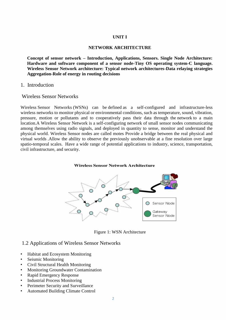
Wireless Sensor Networks (WSNs) can be defined as a self-configured and infrastructure-less
wireless networks to monitor physical or environmental conditions, such as temperature, sound, vibration,
pressure, motion or pollutants and to cooperatively pass their data through the network to a main
location.A Wireless Sensor Network is a self-configuring network of small sensor nodes communicating
among themselves using radio signals, and deployed in quantity to sense, monitor and understand the
physical world. Wireless Sensor nodes are called motes Provide a bridge between the real physical and
virtual worlds .Allow the ability to observe the previously unobservable at a fine resolution over large
spatio-temporal scales. Have a wide range of potential applications to industry, science, transportation,
civil infrastructure, and security.
Figure 1: WSN Architecture
1.2 Applications of Wireless Sensor Networks
• Habitat and Ecosystem Monitoring
• Seismic Monitoring
• Civil Structural Health Monitoring
• Monitoring Groundwater Contamination
• Rapid Emergency Response
• Industrial Process Monitoring
• Perimeter Security and Surveillance
• Automated Building Climate Control

3
• Habitat Monitoring on Great Duck Island
1.2.1 FireBug
Wildfire Instrumentation System Using Networked Sensors.Allows predictive analysis of evolving fire
behavior.Firebugs: GPS-enabled, wireless thermal sensor motes based on TinyOS that self-organize
into networks for collecting real time data in wild fire environments.Software architecture: Several
interacting layers (Sensors, Processing of sensor data, Command center)
1.2.2 Preventive Maintenance on an Oil Tanker in the North Sea: The BP
ExperimentCollaboration of Intel & BP
Use of sensor networks to support preventive maintenance on board an oil tanker in the North Sea. A
sensor network deployment onboard the ship. System gathered data reliably and recovered from errors
when they occurred.
1.2.3 “Cricket” Mote
Basically a location-aware mote. Includes an Ultrasound transmitter and receiver.Uses the combination
of RF and Ultrasound technologies to establish differential time of arrival and hence linear range
estimates.
1.3 TinyOS
TinyOS is an embedded, component-based operating system and platform for low-power wireless
devices, such as those used in wireless sensor networks (WSNs), smartdust, ubiquitous
computing, personal area networks, building automation, and smart meters. It is written in
the programming language nesC, as a set of cooperating tasks and processes. It began as a
collaboration between the University of California, Berkeley, Intel Research, and Crossbow
Technology, was released as free and open-source software under a BSD license, and has since grown
into an international consortium, the TinyOS Alliance.
TinyOS has been used in space, being implemented in ESTCube-1. Low-power sensors, due to their
limitations in scope, require efficient utilization of resources. TinyOS is essentially built on a
“components-based architecture” to reduce code size to around 400 to 500 bytes and an “events-based
design” which eliminates the need for even a command shell. The components-based architecture uses
“nesC,” which is a C programming language designed for networking embedded systems. Each code
snippet consists of simple functions placed within components and complex functions integrating all
the components together.
TinyOS also uses an “events-based design” whose objective is to put the CPU to rest when there are
no pending tasks. An event can be something such as the triggering of an alert when the temperature
of a thermostat rises or falls above a certain value. As soon as the event is over, the sensor motes can
go to sleep.
The need for a design like TinyOS is mandatory in applications such as smart transit and smart
factories. Because of thousands of sensors, it is important to have a very small memory footprint to
reduce power requirements.
4
1.3.1 Applications of TinyOs
Environmental monitoring: since each TinyOS system can be embedded in a small sensor, they are
useful in monitoring air pollution, forest fires, and natural disaster prevention.
Smart vehicles: smart vehicles are autonomous and can be understood as a network of sensors. These
sensors communicate through low-power wireless area networks (LPWAN) which makes TinyOS a
perfect fit.
Smart cities: TinyOS is a viable solution for the low-power sensor requirements of smart cities’
utilities, power grids, Internet infrastructure and other applications.
Machine condition monitoring: machine-to-machine (M2M) applications have many sensor interfaces.
It is impossible to assign a complete computing environment to each sensor. TinyOS can perform
security, power management and debugging of the sensors.
1.3.2 Salient features of TinyOS
A simple event-based concurrency model and split-phase operations that influence the development
phases and techniques when writing application code.
It has a component-based architecture which provides rapid innovation and implementation while
reducing code size as required by the difficult memory constraints inherent in wireless sensor networks.
TinyOS’s component library includes network protocols, distributed services, sensor drivers, and data
acquisition tools.
TinyOS’s event-driven execution model enables fine grained power management, yet allows the
scheduling flexibility made necessary by the unpredictable nature of wireless communication and
physical world interfaces.
1.4 Data Mule
Data mules have been used to offer internet connectivity to remote villages. Computers with a disk and
wifi link are attached to buses on a bus route between villages. As a bus stops at the village to pick up
passengers and cargo, the DTN router on the bus communicates with a DTN router in the bus station
over Wi-Fi. DataMule – a mobile entity present in the environment that will pick up data from the
mote when in range, buffer it, and drop off the data at base station.ex: People, Vehicles, Livestock.Data
mules have been used to offer internet connectivity to remote villages. Computers with a disk and wifi
link are attached to buses on a bus route between villages. As a bus stops at the village to pick up
passengers and cargo, the DTN router on the bus communicates with a DTN router in the bus station
over Wi-Fi. Email is down-loaded to the village and up-loaded for transport to the Internet or to other
villages along the bus route.Data mules are a cost-effective mechanism for rural connectivity because

5
they use inexpensive commodity hardware, can be quickly installed, and can be piggy backed on
existing transportation infrastructure.
1.5 Single Node Architecture
Choosing the hardware components for a wireless sensor node, obviously the applications has to
consider size, costs, and energy consumption of the nodes. A basic sensor node comprises five main
components such as Controller, Memory, Sensors and Actuators, Communication devices and Power
supply Unit.
Figure 2: Single Node Architecture
A controller is used to process all the relevant data, capable of executing arbitrary code. The controller
is the core of a wireless sensor node. It collects data from the sensors, processes this data, decides
when and where to send it, receives data from other sensor nodes, and decides on the actuator’s
behavior. It has to execute various programs, ranging from time critical signal processing and
communication protocols to application programs; it is the Central Processing Unit (CPU) of the
node.For General-purpose processors applications microcontrollers are used.
These are highly overpowered, and their energy consumption is excessive. These are used in
embedded systems. key characteristics of microcontrollers are particularly suited to embedded
systems are their flexibility in connecting with other devices like sensors and they are also convenient
in that they often have memory built in. In a wireless sensor node, DSP could be used to process data
coming from a simple analog, wireless communication device to extract a digital data stream. In
broadband wireless communication, DSPs are an appropriate and successfully used platform.DSP-
specifically geared, with respect to their architecture and their instruction set, for processing large
amounts of vectorial data, as is typically the case in signal processing applications.Memory -to store
programs and intermediate data.Different types of memory are used for programs and data.
In WSN there is a need for Random Access Memory (RAM) to store intermediate sensor readings,
packets from other nodes, and so on. While RAM is fast, its main disadvantage is that it loses its
content if power supply is interrupted. Program code can be stored in Read-Only Memory (ROM) or,
more typically, in Electrically Erasable Programmable Read-Only Memory (EEPROM) or flash
memory (the later being similar to EEPROM but allowing data to be erased or written in blocks
instead of only a byte at a time). Flash memory can also serve as intermediate storage of data in case
6
RAM is insufficient or when the power supply of RAM should be shut down for some time.Turning
nodes into a network requires a device for sending and receiving inform.
Choice of transmission medium:
The communication device is used to exchange data between individual nodes. In some cases, wired
communication can actually be the method of choice and is frequently applied in many sensor
networks. The case of wireless communication is considerably more interesting because it include
radio frequencies. Radio Frequency (RF)- based communication, best fits the requirements of most
WSN applications.
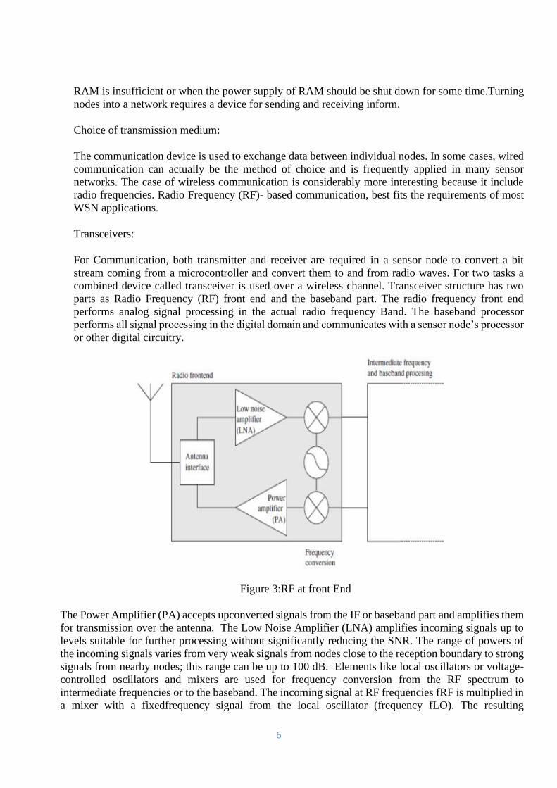
Transceivers:
For Communication, both transmitter and receiver are required in a sensor node to convert a bit
stream coming from a microcontroller and convert them to and from radio waves. For two tasks a
combined device called transceiver is used over a wireless channel. Transceiver structure has two
parts as Radio Frequency (RF) front end and the baseband part. The radio frequency front end
performs analog signal processing in the actual radio frequency Band. The baseband processor
performs all signal processing in the digital domain and communicates with a sensor node’s processor
or other digital circuitry.
Figure 3:RF at front End
The Power Amplifier (PA) accepts upconverted signals from the IF or baseband part and amplifies them
for transmission over the antenna. The Low Noise Amplifier (LNA) amplifies incoming signals up to
levels suitable for further processing without significantly reducing the SNR. The range of powers of
the incoming signals varies from very weak signals from nodes close to the reception boundary to strong
signals from nearby nodes; this range can be up to 100 dB. Elements like local oscillators or voltage-
controlled oscillators and mixers are used for frequency conversion from the RF spectrum to
intermediate frequencies or to the baseband. The incoming signal at RF frequencies fRF is multiplied in
a mixer with a fixedfrequency signal from the local oscillator (frequency fLO). The resulting

7
intermediate frequency signal has frequency fLO − fRF. Depending on the RF front end architecture,
other elements like filters are also present
Transceiver tasks and Characteristics
Service to upper layer: A receiver has to offer certain services to the upper layers, most notably to the
Medium Access Control (MAC) layer. Sometimes, this service is packet oriented; sometimes, a
transceiver only provides a byte interface or even only a bit interface to the microcontroller. Power
consumption and energy efficiency: The simplest interpretation of energy efficiency is the energy
required to transmit and receive a single bit
Carrier frequency and multiple channels: Transceivers are available for different carrier frequencies;
evidently, it must match application requirements and regulatory restrictions. State change times and
energy: A transceiver can operate in different modes: sending or receiving, use different channels, or
be in different power-safe states.Data rates: Carrier frequency and used bandwidth together with
modulation and coding determine the gross data rate.
• Modulations: The transceivers typically support one or several of on/off-keying, ASK, FSK, or similar
modulations.
• Coding: Some transceivers allow various coding schemes to be selected.
• Transmission power control: Some transceivers can directly provide control over the transmission
power to be used; some require some external circuitry for that purpose.
• Usually, only a discrete number of power levels are available from which the actual transmission power
can be chosen. Maximum output power is usually determined by regulations.
• Noise figure: The noise figure NF of an element is defined as the ratio of the Signal-toNoise Ratio
(SNR) ratio SNRI at the input of the element to the SNR ratio SNRO at the element’s output.
• It describes the degradation of SNR due to the element’s operation and is typically given in dB: NF
dB= SNRI dB − SNRO dB
• Gain: The gain is the ratio of the output signal power to the input signal power and is typically given
in dB. Amplifiers with high gain are desirable to achieve good energy efficiency.
• Power efficiency: The efficiency of the radio front end is given as the ratio of the radiated power to
the overall power consumed by the front end; for a power amplifier, the efficiency describes the ratio
of the output signal’s power to the power consumed by the overall power amplifier.
• Receiver sensitivity: The receiver sensitivity (given in dBm) specifies the minimum signal power at
the receiver needed to achieve a prescribed Eb/N0 or a prescribed bit/packet error rate.
• Range: The range of a transmitter is clear. The range is considered in absence of interference; it
evidently depends on the maximum transmission power, on the antenna characteristics.
• Blocking performance: The blocking performance of a receiver is its achieved bit error rate in the
presence of an interferer
• Out of band emission: The inverse to adjacent channel suppression is the out of band emission of a
transmitter. To limit disturbance of other systems, or of the WSN itself in a multichannel setup, the
transmitter should produce as little as possible of transmission power outside of its prescribed
bandwidth, centered around the carrier frequency
• Carrier sense and RSSI: In many medium access control protocols, sensing whether the wireless
channel, the carrier, is busy (another node is transmitting) is a critical information.

8
• The receiver has to be able to provide that information. the signal strength at which an incoming data
packet has been received can provide useful information a receiver has to provide this information in
the Received Signal Strength Indicator (RSSI).
• Frequency stability: The frequency stability denotes the degree of variation from nominal center
frequencies when environmental conditions of oscillators like temperature or pressure change.
• Voltage range: Transceivers should operate reliably over a range of supply voltages. Otherwise,
inefficient voltage stabilization circuitry is required.
1.6 Sensors and Actuators
• The actual interface to the physical world: devices that can observe or control physical parameters of
the environment.Sensors can be roughly categorized into three categories as
• Passive, omnidirectional sensors: These sensors can measure a physical quantity at the point of the
sensor node without actually manipulating the environment by active probing – in this sense, they are
passive. Moreover, some of these sensors actually are self-powered in the sense that they obtain the
energy they need from the environment – energy is only needed to amplify their analog signal.
• Passive, narrow-beam sensors: These sensors are passive as well, but have a well defined notion of
direction of measurement.
• Active sensors: This last group of sensors actively probes the environment, for example, a sonar or
radar sensor or some types of seismic sensors, which generate shock waves by small explosions. These
are quite specific – triggering an explosion is certainly not a lightly undertaken action – and require
quite special attention. Actuators are just about as diverse as sensors
Purposes of designing a WSN - converts electrical signals into physical phenomenon.As usually no
tethered power supply is available, some form of batteries are necessary to provide energy. Sometimes,
some form of recharging by obtaining energy from the environment is available as well (e.g. solar
cells). There are essentially two aspects: Storing energy and Energy scavenging.Traditional batteries:
The power source of a sensor node is a battery, either nonrechargeable (“primary batteries”) or, if an
energy scavenging device is present on the node, also rechargeable (“secondary batteries”).
Requirements of Battery
• Capacity: They should have high capacity at a small weight, small volume, and low price. The main
metric is energy per volume, J/cm3.
• Capacity under load: They should withstand various usage patterns as a sensor node can consume quite
different levels of power over time and actually draw high current in certain operation modes.
• Self-discharge: Their self-discharge should be low. Zinc-air batteries, for example, have only a very
short lifetime (on the order of weeks).
• Efficient recharging: Recharging should be efficient even at low and intermittently available recharge
power
• Relaxation: Their relaxation effect – the seeming self-recharging of an empty or almost empty battery
when no current is drawn from it, based on chemical diffusion processes within the cell – should be
clearly understood. Battery lifetime and usable capacity is considerably extended if this effect is
leveraged.
• DC–DC Conversion: Unfortunately, batteries alone are not sufficient as a direct power source for a
sensor node. One typical problem is the reduction of a battery’s voltage as its capacity drops.
• DC – DC converter can be used to overcome this problem by regulating the voltage delivered to the
node’s circuitry. To ensure a constant voltage even though the battery’s supply voltage drops, the DC

9
– DC converter has to draw increasingly higher current from the battery when the battery is already
becoming weak, speeding up battery death.
• The DC – DC converter does consume energy for its own operation, reducing overall efficiency
Energy Scavenging
• Depending on application, high capacity batteries that last for long times, that is, have only a negligible
self-discharge rate, and that can efficiently provide small amounts of current.
• Ideally, a sensor node also has a device for energy scavenging, recharging the battery with energy
gathered from the environment – solar cells or vibration-based power generation are conceivable
options.
• Photovoltaics: The well-known solar cells can be used to power sensor nodes. The available power
depends on whether nodes are used outdoors or indoors, and on time of day and whether for outdoor
usage.
• The resulting power is somewhere between 10 μW/cm2 indoors and 15 mW/cm2 outdoors. Single
cells achieve a fairly stable output voltage of about 0.6 V (and have therefore to be used in series) as
long as the drawn current does not exceed a critical threshold, which depends on the light intensity.
Hence, solar cells are usually used to recharge secondary batteries.
• Temperature gradients: Differences in temperature can be directly converted to electrical energy.
• Vibrations: One almost pervasive form of mechanical energy is vibrations: walls or windows in
buildings are resonating with cars or trucks passing in the streets, machinery often has low frequency
vibrations. both amplitude and frequency of the vibration and ranges from about 0.1 μW/cm3 up to 10,
000 μW/cm3 for some extreme cases. Converting vibrations to electrical energy can be undertaken by
various means, based on electromagnetic, electrostatic, or piezoelectric principles.
• Pressure variations: Variation of pressure can also be used as a power source.
• Flow of air/liquid: Another often-used power source is the flow of air or liquid in wind mills or
turbines. The challenge here is again the miniaturization, but some of the work on millimeter scale
MEMS gas turbines might be reusable.
Figure 4: MEMS device for converting vibrations to electrical energy, based on a variable capacitor
10
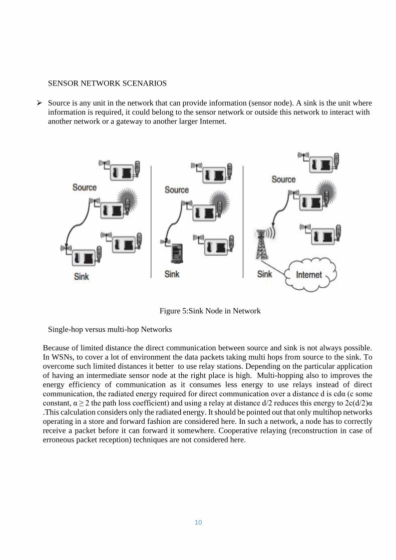
SENSOR NETWORK SCENARIOS
⮚ Source is any unit in the network that can provide information (sensor node). A sink is the unit where
information is required, it could belong to the sensor network or outside this network to interact with
another network or a gateway to another larger Internet.
Figure 5:Sink Node in Network
Single-hop versus multi-hop Networks
Because of limited distance the direct communication between source and sink is not always possible.
In WSNs, to cover a lot of environment the data packets taking multi hops from source to the sink. To
overcome such limited distances it better to use relay stations. Depending on the particular application
of having an intermediate sensor node at the right place is high. Multi-hopping also to improves the
energy efficiency of communication as it consumes less energy to use relays instead of direct
communication, the radiated energy required for direct communication over a distance d is cdα (c some
constant, α ≥ 2 the path loss coefficient) and using a relay at distance d/2 reduces this energy to 2c(d/2)α
.This calculation considers only the radiated energy. It should be pointed out that only multihop networks
operating in a store and forward fashion are considered here. In such a network, a node has to correctly
receive a packet before it can forward it somewhere. Cooperative relaying (reconstruction in case of
erroneous packet reception) techniques are not considered here.

11
Figure 6: Single-hop versus multi-hop Networks
Multiple sinks and sources
⮚ Multiple sources should send information to multiple sinks.
⮚ Either all or some of the information has to reach all or some of the sinks.
Figure 7: Multiple sinks and sources
Types of Mobility
All participants were stationary. But one of the main virtues of wireless communication is its ability
to support mobile participants.In wireless sensor networks, mobility can appear in three main forms

12
a. Node mobility
b. Sink mobility
c. Event mobility
Node Mobility: The wireless sensor nodes themselves can be mobile. The meaning of such mobility
is highly application dependent. In examples like environmental control, node mobility should not
happen; in livestock surveillance (sensor nodes attached to cattle, for example), it is the common rule.
In the face of node mobility, the network has to reorganize to function correctly.
Sink Mobility: The information sinks can be mobile. For example, a human user requested information
via a PDA while walking in an intelligent building. In a simple case, such a requester can interact with
the WSN at one point and complete its interactions before moving on, In many cases, consecutive
interactions can be treated as separate, unrelated requests.
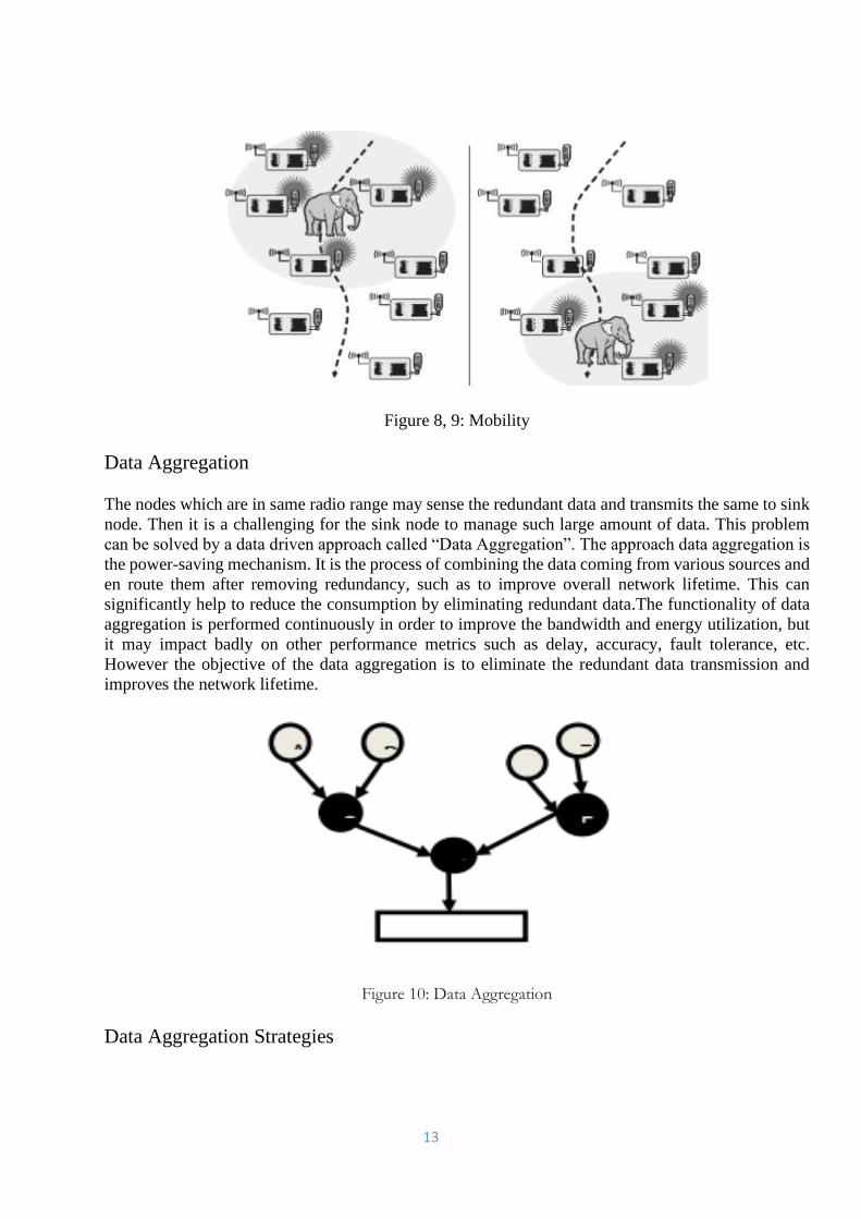
Event Mobility: In tracking applications, the cause of the events or the objects to be tracked can be
mobile. In such scenarios, it is (usually) important that the observed event is covered by a sufficient
number of sensors at all time. As the event source moves through the network, it is accompanied by
an area of activity within the network – this has been called the frisbee model detect a moving elephant
and to observe it as it moves around
Sink mobility: A mobile sink moves through a sensor network as information is being retrieved on its
behalf . Area of sensor nodes detecting an event – an elephant– that moves through the network along
with the event source (dashed line indicate the elephant’s trajectory; shaded ellipse the activity area
following or even preceding the elephant)
•
13
Figure 8, 9: Mobility
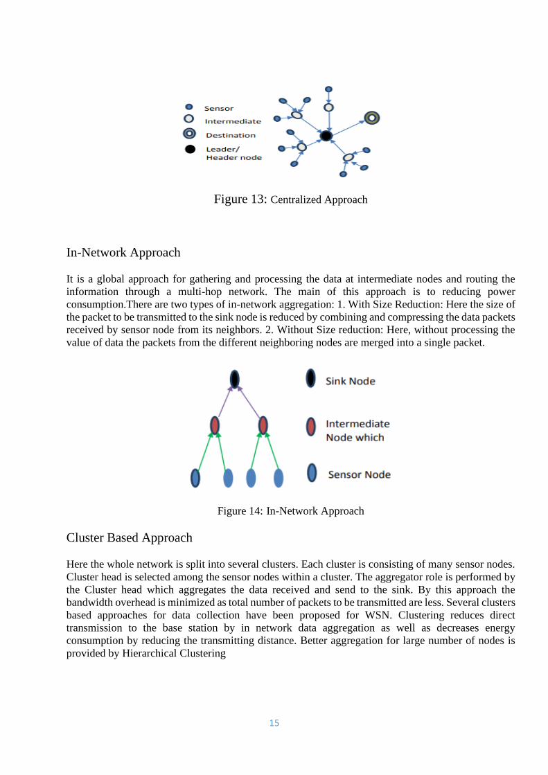
Data Aggregation
The nodes which are in same radio range may sense the redundant data and transmits the same to sink
node. Then it is a challenging for the sink node to manage such large amount of data. This problem
can be solved by a data driven approach called “Data Aggregation”. The approach data aggregation is
the power-saving mechanism. It is the process of combining the data coming from various sources and
en route them after removing redundancy, such as to improve overall network lifetime. This can
significantly help to reduce the consumption by eliminating redundant data.The functionality of data
aggregation is performed continuously in order to improve the bandwidth and energy utilization, but
it may impact badly on other performance metrics such as delay, accuracy, fault tolerance, etc.
However the objective of the data aggregation is to eliminate the redundant data transmission and
improves the network lifetime.
Figure 10: Data Aggregation
Data Aggregation Strategies

14
Figure 11: Data Aggregation Strategies
Tree Based Approach
In this approach, a Data Aggregation Tree (DAT) is framed and here for each data transmission a
minimum spanning tree is constructed. Each node in a network has a parent-child relationship in which
the data is forwarded in a bottom-up approach. The data starts flowing from leaf nodes to the sink node
and the aggregation of the data is done by parent nodes in the network.
Figure 12: Tree Based Approach
Centralized Approach
In this approach each sensor node sends its sensed data to a central node (base station) via the shortest
possible route. All the sensor nodes simply sends the data packets to a node, which is the powerful
among all other nodes This node is called aggregator node or header node. This node aggregates the
data coming from other nodes and the resultant data will be sent as a single packet.
15
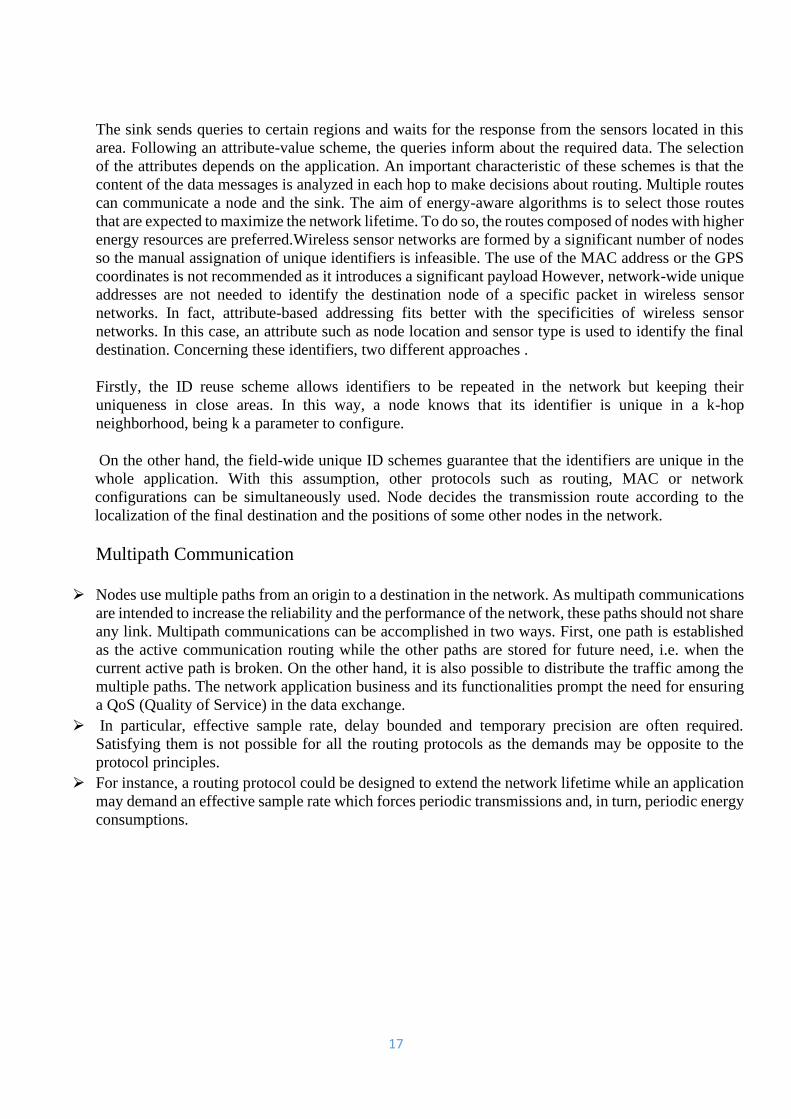
Figure 13: Centralized Approach
In-Network Approach
It is a global approach for gathering and processing the data at intermediate nodes and routing the
information through a multi-hop network. The main of this approach is to reducing power
consumption.There are two types of in-network aggregation: 1. With Size Reduction: Here the size of
the packet to be transmitted to the sink node is reduced by combining and compressing the data packets
received by sensor node from its neighbors. 2. Without Size reduction: Here, without processing the
value of data the packets from the different neighboring nodes are merged into a single packet.
Figure 14: In-Network Approach
Cluster Based Approach
Here the whole network is split into several clusters. Each cluster is consisting of many sensor nodes.
Cluster head is selected among the sensor nodes within a cluster. The aggregator role is performed by
the Cluster head which aggregates the data received and send to the sink. By this approach the
bandwidth overhead is minimized as total number of packets to be transmitted are less. Several clusters
based approaches for data collection have been proposed for WSN. Clustering reduces direct
transmission to the base station by in network data aggregation as well as decreases energy
consumption by reducing the transmitting distance. Better aggregation for large number of nodes is
provided by Hierarchical Clustering

16
Figure 15: Cluster Based Approach
Routing Protocols in WSNs
Figure 16: Routing Protocols in WSNs
Optimization Techniques for Routing in Wireless Sensor Networks
Attribute-based
17
The sink sends queries to certain regions and waits for the response from the sensors located in this
area. Following an attribute-value scheme, the queries inform about the required data. The selection
of the attributes depends on the application. An important characteristic of these schemes is that the
content of the data messages is analyzed in each hop to make decisions about routing. Multiple routes
can communicate a node and the sink. The aim of energy-aware algorithms is to select those routes
that are expected to maximize the network lifetime. To do so, the routes composed of nodes with higher
energy resources are preferred.Wireless sensor networks are formed by a significant number of nodes
so the manual assignation of unique identifiers is infeasible. The use of the MAC address or the GPS
coordinates is not recommended as it introduces a significant payload However, network-wide unique
addresses are not needed to identify the destination node of a specific packet in wireless sensor
networks. In fact, attribute-based addressing fits better with the specificities of wireless sensor
networks. In this case, an attribute such as node location and sensor type is used to identify the final
destination. Concerning these identifiers, two different approaches .
Firstly, the ID reuse scheme allows identifiers to be repeated in the network but keeping their
uniqueness in close areas. In this way, a node knows that its identifier is unique in a k-hop
neighborhood, being k a parameter to configure.
On the other hand, the field-wide unique ID schemes guarantee that the identifiers are unique in the
whole application. With this assumption, other protocols such as routing, MAC or network
configurations can be simultaneously used. Node decides the transmission route according to the
localization of the final destination and the positions of some other nodes in the network.
Multipath Communication
⮚ Nodes use multiple paths from an origin to a destination in the network. As multipath communications
are intended to increase the reliability and the performance of the network, these paths should not share
any link. Multipath communications can be accomplished in two ways. First, one path is established
as the active communication routing while the other paths are stored for future need, i.e. when the
current active path is broken. On the other hand, it is also possible to distribute the traffic among the
multiple paths. The network application business and its functionalities prompt the need for ensuring
a QoS (Quality of Service) in the data exchange.
⮚ In particular, effective sample rate, delay bounded and temporary precision are often required.
Satisfying them is not possible for all the routing protocols as the demands may be opposite to the
protocol principles.
⮚ For instance, a routing protocol could be designed to extend the network lifetime while an application
may demand an effective sample rate which forces periodic transmissions and, in turn, periodic energy
consumptions.

18
Figure 17: WSN Vs QOS Metrics
Significance for Study of Energy in Wireless Sensor Networks
To evaluate the network performance, consider parameters that evidence proper network operation
directly influencing the energy consumption of each node. There are local and global parameters.
Global parameters display the total energy costs for the network considering each type of energy for
each specific activity. In contrast, local parameters provide total energy consumption rates for a single
node. This energy depends on the location of the node within the topology regardless of how near or
far they are located from the coordinator node and how much traffic is transmitted through it
An energy-efficient routing protocol decreases the consumption of the nodes by routing data through
paths that display the least amount of energy. There are some special mechanisms to achieve this goal
such as optimization of jumps to the destination node, maintenance of optimal and valid routes,
reduction of transmission delays, and reduction of packet retransmissions and attempts to listen to the
channel.Concerning the communication channel, it is a factor that significantly influences the energy
consumption because the protocol executes a series of listening attempts to determine whether the
channel is already busy with other information packets. The carrier senses multiple accesses with the
collision avoidance (CSMA/CA) protocol.first, a node begins listening to the wireless channel and if
it is free, the node begins transmitting. If the wireless channel is not free, the node recalculates a
random delay, waits, and listens again. MAC-level protocol is used for all extensions of 802.15.4
(including the original version), which is the CSMA/CA that guarantees a high data rate.
A network recognition is being carried out at all times to check the status of the channel (carrier
detection). Only when free, data can be sent. In the 802.11 standard, the physical layer polls the energy
level over the radio frequency to determine whether or not there is transmission. If the channel is busy,
a random timer starts (with a maximum of five back off periods), the timer only discovers time with
free channel, transmits when it expires, and finally, if it does not receive ACK, it increases the back
off. This metric is known as CSMA/CA retries. If these CSMA/CA retries are frequent, the channel is
busy most of the time. Consequently, there might be several collisions due to overload. In addition,
when the wireless channel is permanently busy with information packets, there are many collisions
and retransmissions of packets. This fact influences energy consumption because the nodes spend more
time and capacity retransmitting over and over.In a network layer, overloads are an important factor
that influence energy consumption.
The efficiency of the routing protocol may also be measured by the number of packets the protocol
needs to route to its destination. A protocol with many control packets will contribute to packet

19
collisions and overall performance reduction. In terms of route discovery, in all the protocols
considered, the nodes exhibit capacity to know their neighbors.
Network energy consumption is directly related to the complexity in the administration of routing or
neighbor tables. As sensors execute huge routing processes, energy consumption increases if these
routes have not been properly updated. This is why it is also important to assess route delays; they are
directly related to the number of jumps that a node takes to reach a destination.

20
SCHOOL OF COMPUTING
DEPARTMENT OF COMPUTER SCIENCE AND ENGINEERING
Unit- II- WIRELESS SENSOR NETWORKS-SCSA5202
21
Unit 2
MAC LAYER
MAC Layer Strategies: MAC Layer Protocols-Scheduling Sleep Cycles-Energy Management-
Contention Based ProtocolsSchedule Based Protocols, 802.15.4 Standard. Naming and
Addressing: Addressing Services - Publish-Subscribe Topologies. Clock Synchronization:
Clustering For Synchronization-Sender-Receiver-Receiver Synchronization-Error Analysis.
Power Management – Per Node -System-Wide-Sentry Services-Sensing Coverage
The wireless medium being inherently broadcast in nature and hence prone to interferences requires
highly optimized medium access control (MAC) protocols. The prime role of the MAC is to coordinate
access to and transmission over a medium common to several nodes
Issues in designing MAC protocol for Sensor networks
1. Bandwidth Efficiency
It is defined as the ratio of the bandwidth utilized for data transmission to the total available bandwidth.
Bandwidth must be utilized in efficient manner. Control-overhead must be kept as minimal as possible.
2. Quality of Service support
This is essential for supporting time-critical traffic-sessions. • The protocol should have resource
reservation mechanism that takes into considerations. 1) Nature of wireless-channel and 2) Mobility
of nodes
3. Synchronization • This is very important for bandwidth (time-slot) reservation by nodes. • The
protocol must consider synchronization between nodes in the network. • Exchange of control-packets
may be required for achieving timesynchronization among nodes.
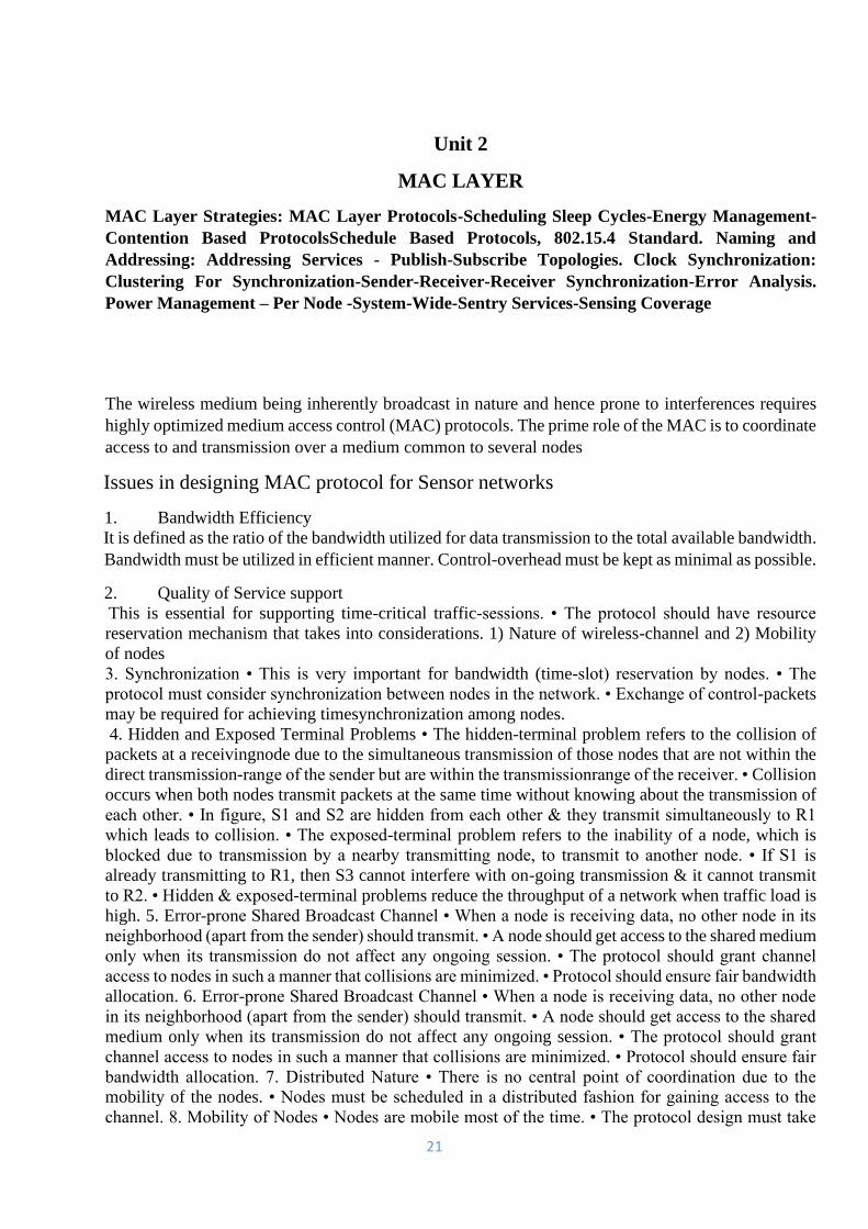
4. Hidden and Exposed Terminal Problems • The hidden-terminal problem refers to the collision of
packets at a receivingnode due to the simultaneous transmission of those nodes that are not within the
direct transmission-range of the sender but are within the transmissionrange of the receiver. • Collision
occurs when both nodes transmit packets at the same time without knowing about the transmission of
each other. • In figure, S1 and S2 are hidden from each other & they transmit simultaneously to R1
which leads to collision. • The exposed-terminal problem refers to the inability of a node, which is
blocked due to transmission by a nearby transmitting node, to transmit to another node. • If S1 is
already transmitting to R1, then S3 cannot interfere with on-going transmission & it cannot transmit
to R2. • Hidden & exposed-terminal problems reduce the throughput of a network when traffic load is
high. 5. Error-prone Shared Broadcast Channel • When a node is receiving data, no other node in its
neighborhood (apart from the sender) should transmit. • A node should get access to the shared medium
only when its transmission do not affect any ongoing session. • The protocol should grant channel
access to nodes in such a manner that collisions are minimized. • Protocol should ensure fair bandwidth
allocation. 6. Error-prone Shared Broadcast Channel • When a node is receiving data, no other node
in its neighborhood (apart from the sender) should transmit. • A node should get access to the shared
medium only when its transmission do not affect any ongoing session. • The protocol should grant
channel access to nodes in such a manner that collisions are minimized. • Protocol should ensure fair
bandwidth allocation. 7. Distributed Nature • There is no central point of coordination due to the
mobility of the nodes. • Nodes must be scheduled in a distributed fashion for gaining access to the
channel. 8. Mobility of Nodes • Nodes are mobile most of the time. • The protocol design must take

22
this mobility factor into consideration so that the performance of the system is not affected due to node
mobility.
Figure 1: Hidden and Exposed Terminal
MAC Layer Protocols
There are two main categories of MAC protocols for WSNs, according to how the MAC manages when
certain nodes can communicate on the channel:
• Time-division multiple access (TDMA) based: These protocols assign different time slots to nodes.
Nodes can send messages only in their time slot, thus eliminating contention. Examples of this kind
of MAC protocols include LMAC, TRAMA, etc.
• Carrier-sense multiple access (CSMA) based: These protocols use carrier sensing and backoffs to
avoid collisions, similarly to IEEE 802.11. Examples include B-MAC, SMAC, TMAC, X-MAC.
B-MAC
B-MAC (short for Berkeley MAC) is a widely used WSN MAC protocol; it is part of TinyOS. It employs
low-power listening (LPL) to minimize power consumption due to idle listening. Nodes have a sleep period,
after which they wake up and sense the medium for preambles (clear channel assessment - CCA.) If none is
detected, the nodes go back to sleep. If there is a preamble, the nodes stay awake and receive the data packet
after the preamble. If a node wants to send a message, it first sends a preamble for at least the sleep period in
order for all nodes to detect it. After the preamble, it sends the data packet. There are optional
acknowledgments as well. After the data packet (or data packet + ACK) exchange, the nodes go back to sleep.
Note that the preamble doesn’t contain addressing information. Since the recipient’s address is contained in
23
the data packet, all nodes receive the preamble and the data packet in the sender’s communication range (not
just the intended recipient of the data packet.)
X-MAC
X-MAC is a development on B-MAC and aims to improve on some of B-MAC’s shortcomings. In B-MAC,
the entire preamble is transmitted, regardless of whether the destination node awoke at the beginning of the
preamble or the end. Furthermore, with B-MAC, all nodes receive both the preamble and the data packet. X-
MAC employs a strobed preamble, i.e. sending the same length preamble as B-MAC, but as shorter bursts,
with pauses in between. The pauses are long enough that the destination node can send an acknowledgment if
it is already awake. When the sender receives the acknowledgment, it stops sending preambles and sends the
data packet. This mechanism can save time because potentially, the sender doesn’t have to send the whole
length preamble. Also, the preamble contains the address of the destination node. Nodes can wake up, receive
the preamble, and go back to sleep if the packet is not addressed to them. These features improve B-MAC’s
power efficiency by decreasing nodes’ time spent in idle listening.
LMAC
LMAC (short for lightweight MAC) is a TDMA-based MAC protocol. There are data transfer timeframes,
which are divided into time slots. The number of time slots in a timeframe is configurable according to the
number of nodes in the network. Each node has its own time slot, in which only that particular node can
transmit. This feature saves power, as there are no collisions or retransmissions. A transmission consists of a
control message and a data unit. The control message contains the destination of the data, the length of the
data unit, and information about which time slots are occupied. All nodes wake up at the beginning of each
time slot. If there is no transmission, the time slot is assumed to be empty (not owned by any nodes), and the
nodes go back to sleep. If there is a transmission, after receiving the control message, nodes that are not the
recipient go back to sleep. The recipient node and the sender node goes back to sleep after receiving/sending
the transmission. Only one message can be sent in each time slot. In the first five timeframes, the network is
set up and no data packets are sent. The network is set up by nodes claiming a time slot. They send a control
message in the time slot they want to reserve. If there are no collisions, nodes note that the time slot is claimed.
If there are multiple nodes trying to claim the same time slot, and there is a collision, they randomly choose
another unclaimed time slot.
The INET implementations
The three MACs are implemented in INET as the BMac, XMac, and LMac modules. They have parameters
to adapt the MAC protocol to the size of the network and the traffic intensity, such as slot time, clear channel
assessment duration, bitrate, etc. The parameters have default values, thus the MAC modules can be used
without setting any of their parameters. Check the NED files of the MAC modules (BMac.ned, XMac.ned,
and LMac.ned) to see all parameters.
24
The MACs don’t have corresponding physical layer models. They can be used with existing generic radio
models in INET, such as UnitDiskRadio or ApskRadio.
Configuration
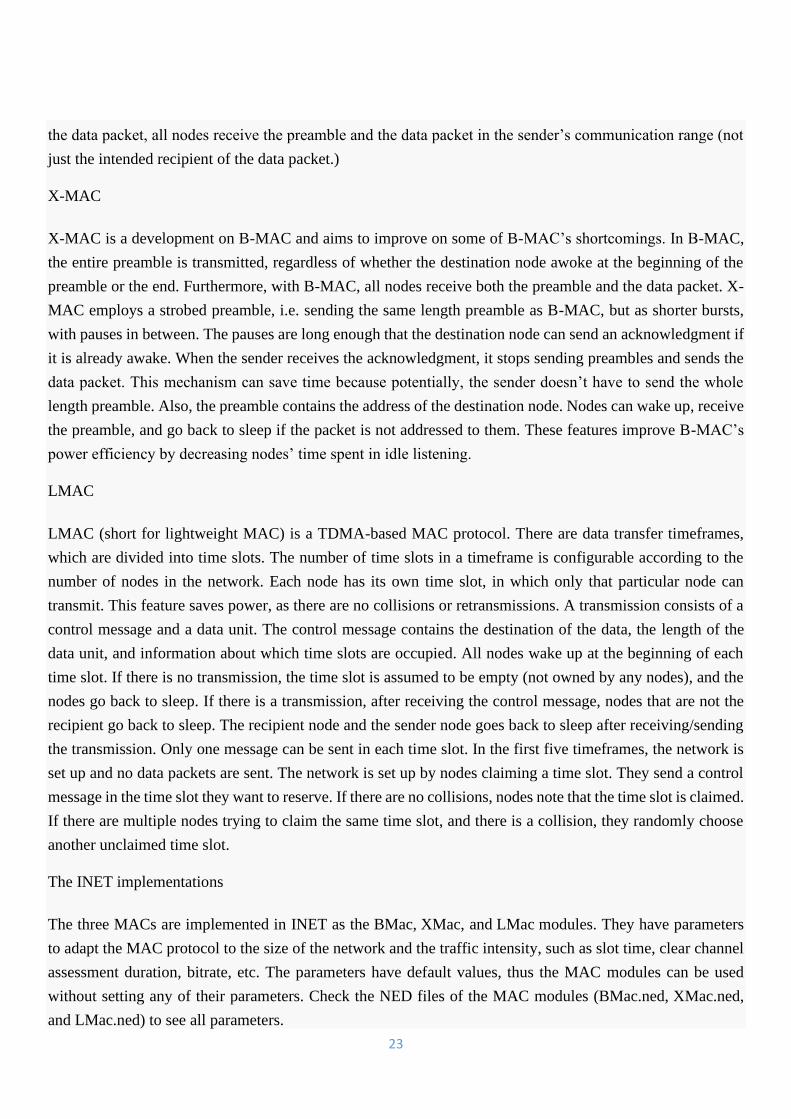
The showcase contains three example simulations, which demonstrate the three MACs in a wireless sensor
network. The scenario is that there are wireless sensor nodes in a refrigerated warehouse, monitoring the
temperature at their location. They periodically transmit temperature data wirelessly to a gateway node, which
forwards the data to a server via a wired connection.
Note that in WSN terminology, the gateway would be called sink. Ideally, there should be a specific
application in the gateway node called sink, which would receive the data from the WSN, and send it to the
server over IP. Thus the node would act as a gateway between the WSN and the external IP network. In the
example simulations, the gateway just forwards the data packets over IP.
Figure 2:Sensor sending data to gateway
In the network, the wireless sensor nodes are of the type SensorNode, named sensor1 up to sensor4,
and gateway. The node named server is a StandardHost. The network also contains
an Ipv4NetworkConfigurator, an IntegratedVisualizer, and an ApskScalarRadioMedium module. The nodes
are placed against the backdrop of a warehouse floorplan. The scene size is 60x30 meters. The warehouse is
just a background image providing context. Obstacle loss is not modeled, so the background image doesn’t
affect the simulation in any way. Routes are set up according to a star topology, with the gateway at the center.
This is achieved by dumping the full configuration of Ipv4NetworkConfigurator (which was generated with
the configurator’s default settings), and then modifying it. The modified configuration is in the config.xml file.
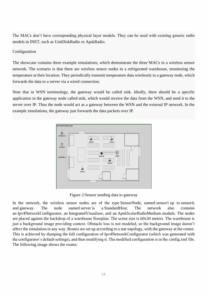
The following image shows the routes:
25
Figure 3: Bidirectional data transfer
Each sensor node will send an UDP packet with a 10-byte payload (“temperature data”) every second to the
server, with a random start time around 1s. The packets will have an 8-byte UDP header and a 20-byte Ipv4
header, so they will be 38 bytes at the MAC level. The packets will be routed via the gateway.The MAC-specific
parameters are set in the configurations for the individual MACs.
For B-MAC, the wireless interface’s macType parameter is set to BMac. Also, the slotDuration parameter is
set to 0.025s (an arbitrary value.) This parameter is essentially the nodes’ sleep duration.
For X-MAC, the wireless interface’s macType parameter is set to XMac. The MAC’s slotDuration parameter
determines the duration of the nodes’ sleep periods. It is set to 0.25s for the sensor nodes and 0.1s for the
gateway. Nodes transmit preambles for the duration of their own sleep periods unless interrupted by an
acknowledgment from the destination node. The design of X-MAC allows setting different sleep intervals for
different nodes, as long as the sender node’s sleep interval is greater than the receiver’s. (?). We set the slot
duration of the gateway to a shorter value because it has to receive and relay data from all sensors, thus it has
more traffic.
For LMAC, the wireless interface’s macType parameter is set to LMac. The numSlots parameter is set to 8,
as it is sufficient (there are only five nodes in the wireless sensor network.)
The reservedMobileSlots parameter reserves some of the slots for mobile nodes; these slots are not chosen by
any of the nodes during network setup. The parameter’s default value is 2, but it is set to 0.
The slotDuration parameter’s default value is 100ms, but we set it to 50ms to decrease the network setup time.
The duration of a timeframe will be 400ms (number of slots * slot duration.) The network is set up in the first
five frames, i.e. in the first 2 seconds.
Traditional MAC Families
There are two main approaches for regulating access to a shared wireless medium:
• Contention-based
• Reservation based approaches.
26
Reservation-Based Protocols
• Requires the knowledge of the network topology to establish a schedule that allows each node to access
the channel and communicate with other nodes.
• The schedule may have various goals such as ensuring fairness among nodes, or reducing collisions
by avoiding that two interfering nodes or more access to the channel and transmit at the same time.
• TDMA (Time Division Multiple Access) is a representative example for such a reservation-based
approach.
• In TDMA, time is divided into frames and each frame is divided into slots.
• During a frame, each node is assigned a unique slot during which it has the right to transmit.
• As a consequence, transmissions do not suffer from collisions , which guarantees finite and predictable
scheduling delays and also increases the overall throughput in highly loaded networks.
• The throughput is usually hard-limited, i.e. it cannot be increased beyond the utilization of all available
slots. TDMA schemes also ensure fairness among nodes as each node is assigned a unique slot in each
frame.
Contention-Based Protocols
• Neither global synchronization nor topology knowledge is required.
• In a contention-based approach, nodes compete for the use of the wireless medium and only the winner
of this competition is allowed to access to the channel and transmit.
• ALOHA and CSMA (Carrier Sense Multiple Access) are canonical representative schemes of
contentionbased approaches
• In CSMA, for instance, a node having a packet to transmit first senses the channel before actually
transmitting.
• In the case that the node finds the channel busy, it postpones its transmission to avoid interfering with
the ongoing transmission.
• In the other case that the node finds the channel clear, it starts transmitting (after possibly having
waited a random time).
• CSMA does not rely on a central entity and is robust to node mobility, which makes it intuitively a
good candidate for networks with mobility and dynamicity

27
Figure 4: Contention Based Protocol
Design-Drivers for WSN- MAC Protocols
The design of MAC protocols for WSNs is mainly impacted by a high energy constraint but also by a low
complexity of the nodes, their low computational capabilities and low memory footprints as well as poor
synchronization capabilities. A functional MAC for WSNs hence ought to be highly energy efficient but also
ensure high reliability, low access delay and throughput given above impairments.
Challenges for MAC
1. Collisions. They may happen when a node is within the transmission range of two or more nodes that are
simultaneously transmitting so that it does not capture any frame.The energy drained in the transmission
and reception of collided frames is just wasted. Due to the large impact of collisions on protocols
performance, MAC protocols should feature techniques to reduce or even avoid them
2. Overhearing.
It happens when a node drains energy receiving irrelevant packets or signals. Irrelevant packets may be for
example unicast packets destined to other nodes or redundant broadcast packets.Irrelevant signals
include the preambles used in some low power MAC protocols to occupy the communication channel
3. Overhead.
Protocol overhead may result in energy waste when transmitting and receiving control packets. For example,
RTS and CTS control packets used in some protocols do not carry any useful data to applications although
their transmission consumes energy. For example, the exchange of RTS/CTS induces high overheads in
the range of 40% to 75% of the channel capacity, because data frames are typically very small in sensor
networks
4. Idle Listening. It happens when a node does not know when it will be the receiver of a frame, which is
generally the situation. In this case, the node keeps its radio on while listening to the channel waiting for

28
potential data frames. The amount of energy wasted whilst the radio is on is considerable even when it is
neither receiving nor transmitting frames
Sleep Scheduling
• Sleep scheduling is a widely used mechanism in wireless sensor networks (WSNs) that can save the
energy wastage caused by the idle listening state by reducing the energy consumption.
• In sleep scheduling, sender nodes should wait until the receiver nodes are in active state and ready to
receive the message. Sleep scheduling increases the network lifetime but it could cause transmission
delay.
• Increase in network scale increases the broadcasting delays.
• So in order to provide low broadcasting delay from any node in the WSN, a delay aware sleep
scheduling method needs to be designed.
• Most of the sleep scheduling methods is introduced to minimize the energy consumption.
• The destination node should wake up immediately when the source nodes obtain the broadcasting
packets.
• Whenever a critical event occurs, it is detected by the nearby sensor nodes and immediately it should
have sent to its neighbor nodes
Components of sleep scheduling protocol
Target prediction
Target prediction scheme propose three steps: current state calculation, kinematics- based prediction
and probability based prediction. After the current state calculation, the kinematics based prediction
step is used to calculate the expected displacement from the current location within the next sleep
delay, and the probability models for scalar displacement and the derivation.
Awakened node reduction
• The number of awakened nodes can be minimized by two efforts: controlling the scope of awakened
regions, and by choosing a subset of nodes in an awakened region.
• Active time
Based on the probabilistic models the prediction scheduling can be done to make the particular node
to be active, so that the probability that it detects to target is close to 1.
Energy Efficient TDMA Sleep Scheduling
29
In a traditional sleep scheduling, sensors have to start up numerous times in a period, and thus consume
extra energy due to the state transitions. In energy efficient sleep scheduling, sensors not only consume
various amounts of energy in various states (transmit, receive, idle and sleep), but also consume energy
for state transitions.TDMA as the MAC layer protocol is used so that it has the advantages of avoiding
collisions, idle listening and overhearing. The energy efficient TDMA protocols allocate time slots to
sensor nodes. These slots are assigned to switch off the radio when not transmitting or receiving in the
sleep scheduling and switch on the radio during the assigned time slots.
In order to be interference free, the number of time slots should be equal to the number of communication
links of the network. To achieve this a simple approach is to assign each communication link a time slot.
This method requires much more time slots than necessary, which reduces the channel utilization and
increases the delay significantly. This is because multi-hop networks are able to make multiple
transmissions that can be scheduled in one-time slot without any interference and space reuse in the shared
channel. To minimize the number of time slots TDMA link scheduling is used while producing an
interference-free link scheduling, and it has been shown that the problem is NP-complete. However, if
the TDMA link scheduling is used as the start of mechanism in the scheduling with sleep mode, a node
may start up numerous times to communicate with its neighbors. The Important factor to be noticed is
that the startup time here is in the order of milliseconds, while the transmission time if the packets are
small may be less than transmission time.
Consequently, the transitory energy consumption during the startup process can be higher than the energy
during the actual transmission. Due to frequent starting up of sensor node, it not only takes extra time, but also
costs extra energy for the state transition. Therefore, the state transformation, for instance from the sleep mode
to the active mode, should be considered for an energy efficient TDMA sleep scheduling in WSNs Merits: 1)
Maximizes the life of wireless sensor network. 2) Reduces packet loss during Sleep Scheduling. 3) Avoids
collisions, idle listening and overhearing
• Demerits: 1) This method requires much more time slots, which significantly increases the delay and
reduces the channel utilization.
• 2) Overlapping of data may occur in this technique
Balanced-energy Sleep Scheduling
The sleeping techniques are widely used to conserve energy of battery powered sensors. Rotating active
and inactive modes of the sensors in the cluster, some of which provide redundant data, is one way that
sensors can be efficiently managed to extend network lifetime.In order to extend the network lifetime some
researchers suggest putting redundant sensor nodes into the network and allowing the extra sensors to
sleep. This is possible made due to the low cost of individual sensors.
When the sensor node is in a sleep state, it completely shuts itself down, leaving only one extremely low
power timer to be on to wake itself up at a later time. The energy costs of both computation and
communication activities were considered in the task allocation problems for wireless networked
embedded systems with homogeneous elements. However, determining which of the sensor nodes should
be put into the sleep state is essential.
This can be achieved by analyzing a Balanced-energy Scheduling (BS) scheme in the context of cluster-
based sensor networks. In BS scheme, it evenly distributes the energy load of the sensing and

30
communication tasks among all the sensor nodes in the cluster, thereby extending the time until the cluster
can no longer provide enough sensing coverage. The BS scheme extends the cluster's overall network
lifetime significantly by maintaining a similar sensing coverage compared with the DS and the RS schemes
for sensor clusters
• Merits: 1) Extends the network Lifetime by using redundant sensors. 2) Balances the load in network
thereby improving the efficiency of the WSN Network.
• Demerits: 1) While balancing the load in network, passing data to long distance become difficult
because some route requires more energy and some route require less energy.
Optimal Sleep Scheduling
A wireless sensor network nodes sleep periodically to maintain the energy level; however, rather than
analyzing the system with a given sleep control policy; e impose a cost structure and search for an optimal
policy among a class of policies. In order to approach the problem in this manner, it is necessary to consider
a far simpler system than those used in the already mentioned studies.Here only a single sensor node is
considered and focused on the tradeoffs between energy consumption and packet delay.As such, quality
of service measures such as connectivity or coverage is not taken in account.
The single node that is focused has the option of turning its transmitter and receiver off for fixed durations
of time in order to conserve energy. Doing so certainly results in additional packet delay. It is experimented
to identify the manner in which the optimal sleep schedule differs with the length of the sleeping period,
the arriving packets statistics, the charges calculated for energy consumption and packet delay.The final
result is a flexible framework in which application designers can trade-off energy versus latency of event
detection
• Merits: 1) This technique is used to minimize the Communication delay. 2) Optimal sleep scheduling
improves the lifetime of the WSN.
• Demerits: 1) This technique does not maintain the quality of service such as connectivity or
coverage
Dynamic Sleep Scheduling
The dynamic sleep energy conservation is important during the periods of no activity and also during the
occurrence of events. Since the transceiver consumes similar energy for idle listening as transmission, it
is critical to reduce traffic overhearing. The overhearing can be minimized if nodes can determine when
they are expected to send and receive packets.Although sleep-scheduling in wireless sensor networks has
been an active area of research, scheduling to reduce the energy conservation for nodes carrying traffic
has not received much attention. MAC layer protocols usually lead to low throughput and high event
reporting latency by putting nodes to low duty-cycle.
While for some applications like event tracking, besides energy saving throughput and latency are also
important metrics. To save energy on nodes carrying traffic, TDMA based link scheduling is widely used
to put nodes to sleep when they are idle while it is in the way of traffic. Based on information collected
from all links the per-packet scheduling is performed. Excessive messaging is necessary for the global
coordination which cause delays in link scheduling.TRAMA is traffic adaptive medium access protocol
which proposes distributed scheduling at each node based on information collected within a fixed number

31
of hops. This minimizes the limitation of centralized scheduling. Although TRAMA can reduce energy
conservation, the conservative local coordination results in exceed of latencies 100 times the latency of
CSMA based approaches. Therefore, TRAMA is not useful in scenarios where latency and throughput are
the critical metrics of performance, which is hardly the case in most wireless sensor networks
• Merits: 1) Avoids the packet loss. 2) Dynamic sleep scheduling used with the MAC layer improves
the high throughput.
• Demerits: 1) Controlling the traffic is very difficult. 2) Data loss in large network.
Delay Efficient Sleep Scheduling
Wireless sensor networks (WSN) are expected to work for months if not years with limited lifetimes on
small inexpensive batteries. Typically, the primary goal of these networks is energy efficiency. Previous
studies have identified that idle listening conserves more energy. A measurement on existing sensor device
shows that the idle listening consumes nearly the same energy as receiving. In sensor network applications
where the traffic load is very light most of the time, it is desirable to turn off the radio when a node does
not participate in any data delivery. In order to reduce the idle listening energy, cost the S-MAC is used to
introduce synchronized periodic duty cycles of nodes.
In S-MAC each node undergoes a periodic active/sleep state, synchronized with its neighboring nodes.
During sleep state, the radios are completely turned off, and they are turned back on during active periods
to transmit and receive messages.Although the synchronized low duty cycle process of a sensor network
is energy efficient; it has one major deficiency of increase in packet delivery latency. At a source node,
during the sleep period a sampling reading may occur and until the active period it has to be queued. Until
the receiver wakes up an intermediate node may have to wait to forward a packet received. This approach
provides some reduction in sleep latency at the expense of greater energy due to extended overhearing and
activation, but not for long paths. An alternate approach designed particularly for wireless sensor networks
where the communication pattern is restricted to an established unidirectional data gathering tree is the
delay-efficient sleep scheduling.
In this case, the sleep latency can be essentially eliminated by having a periodic receive-transmit-sleep
cycle with level-by-level offset schedules, where the data cascades in step by step from the leaves of the
tree towards the sink. The nodes go to sleep as soon as they transmit their packets to the next level, and
wakes up just in time to receive the next round of packets
• Merits: 1) Avoids collision during broadcasting in WSN. 2) Reduces the Energy Consumption and
delay in communication.
• Demerits: 1) Difficult to minimize the Delay in communication while broadcasting the message. 2)
Difficult to maintain latency parameter.
Names vs. Addresses
• Names: Refer to “things”
• Nodes, networks, data, transactions, …
• May or may not be globally unique

32
• Addresses: Information needed to find these things
• Street address, IP address, MAC address
• May or may not be globally unique
• Services to map between names and addresses
• E.g., DNS
• Some names are also addresses
• Nodes are not independent
• But collaborate to solve a given task
• Better to shift view from naming nodes to naming data
Address Management Issues
• Address allocation: Assign an entity an address from a given pool of possible addresses
• Distributed address assignment (centralized like DHCP does not scale)
• Address deallocation: Once address no longer used, put it back into the address pool
• Because of limited pool size
• Graceful or abrupt, depending on node actions
• Address representation
• Conflict detection & resolution (Duplicate Address Detection - DAD)
• What to do when the same address is assigned multiple times?
• Can happen e.g. when two networks merge
• Binding
• Map between addresses used by different protocol layers
• E.g., IP addresses are bound to MAC address by ARP
Uniqueness of Addresses
• Globally unique
• Appears at most once all over the world
• Network-wide unique
• Appears at most once in a given network
• Locally unique
• Appears at most once in a defined neighborhood
Addressing Overhead
33
• The fewer bits per address, the better
• Global > Network-wide > Local
• Tradeoffs
• Address length management overhead
• Typically, address negotiation runs only at the beginning
• Except when there is mobility
Distributed Address Assignment
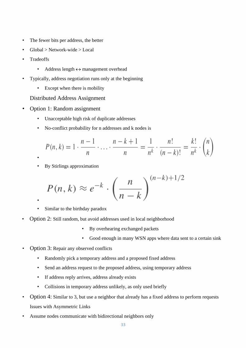
• Option 1: Random assignment
• Unacceptable high risk of duplicate addresses
• No-conflict probability for n addresses and k nodes is
•
• By Stirlings approximation
•
• Similar to the birthday paradox
• Option 2: Still random, but avoid addresses used in local neighborhood
• By overhearing exchanged packets
• Good enough in many WSN apps where data sent to a certain sink
• Option 3: Repair any observed conflicts
• Randomly pick a temporary address and a proposed fixed address
• Send an address request to the proposed address, using temporary address
• If address reply arrives, address already exists
• Collisions in temporary address unlikely, as only used briefly
• Option 4: Similar to 3, but use a neighbor that already has a fixed address to perform requests
Issues with Asymmetric Links
• Assume nodes communicate with bidirectional neighbors only
34
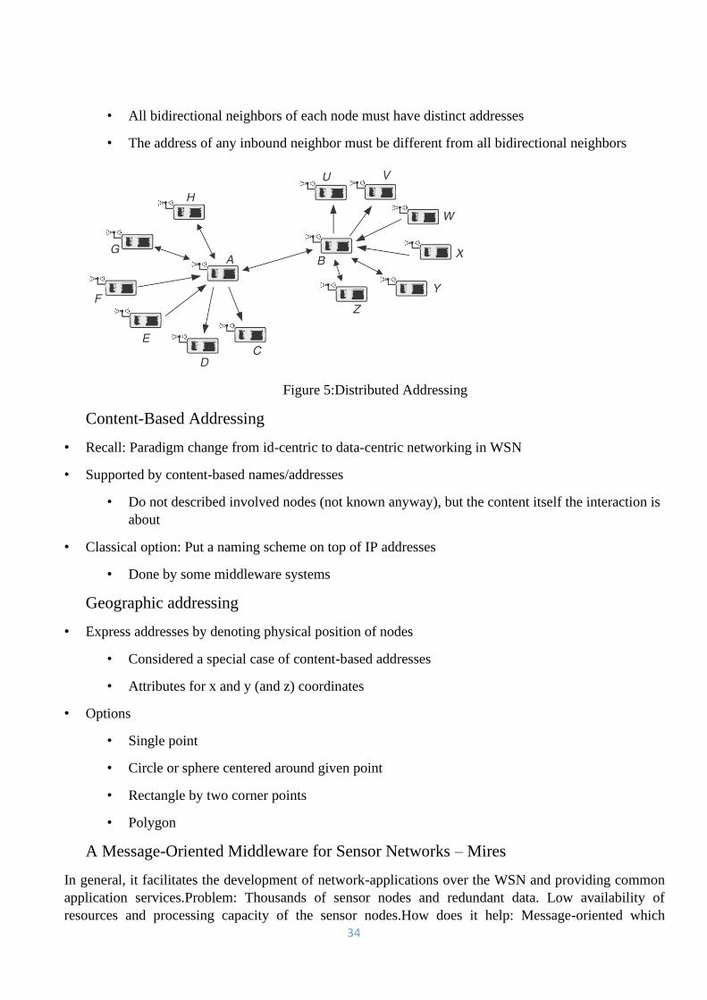
• All bidirectional neighbors of each node must have distinct addresses
• The address of any inbound neighbor must be different from all bidirectional neighbors
Figure 5:Distributed Addressing
Content-Based Addressing
• Recall: Paradigm change from id-centric to data-centric networking in WSN
• Supported by content-based names/addresses
• Do not described involved nodes (not known anyway), but the content itself the interaction is
about
• Classical option: Put a naming scheme on top of IP addresses
• Done by some middleware systems
Geographic addressing
• Express addresses by denoting physical position of nodes
• Considered a special case of content-based addresses
• Attributes for x and y (and z) coordinates
• Options
• Single point
• Circle or sphere centered around given point
• Rectangle by two corner points
• Polygon
A Message-Oriented Middleware for Sensor Networks – Mires
In general, it facilitates the development of network-applications over the WSN and providing common
application services.Problem: Thousands of sensor nodes and redundant data. Low availability of
resources and processing capacity of the sensor nodes.How does it help: Message-oriented which

35
aggregate data, Multi-Hop routing and greatly reduce the among of transmissions, save lots of
energy.Traditional request/response approach is not suitable for event-driven communication model.
Publish/subscribe approach is used to query and extract data from the network.In applications: Use in
habitat monitoring, object tracking, precision agriculture, building monitoring and military systems.
MIRES Architecture
• Publish/Subscribe service
• communication between middleware services.
• Advertising the topics available.
• Maintaining the list of topics subscribed by the node application
• Publishing messages.
• Routing
• Multi-hop routing to the Sink
• 3 types of notification events:
• TopicArrival,
• event signals that the node application has submitted data collected from sensors.
• StateArrival
• Event signals that data received from the network.
• TopicSetupArrival
• the subscribe message broadcasted from the user application.
Figure 6:MIRES Architecture
Publish/Subscribe Service
• PublishState interface define the command used by ServiceX to publish their processing results.
• Notifier interface defines 3 events
• MultiHopRouter-route to the sink

36
• BCast-Boardcast Setup info.
Figure 7: Publish Service
Figure 8: Advertisement
Figure 9: Subscibe Service
37
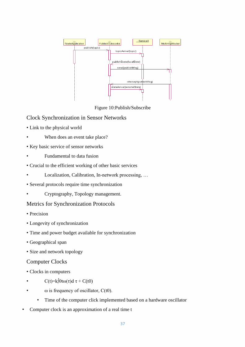
Figure 10:Publish/Subscribe
Clock Synchronization in Sensor Networks
• Link to the physical world
• When does an event take place?
• Key basic service of sensor networks
• Fundamental to data fusion
• Crucial to the efficient working of other basic services
• Localization, Calibration, In-network processing, …
• Several protocols require time synchronization
• Cryptography, Topology management.
Metrics for Synchronization Protocols
• Precision
• Longevity of synchronization
• Time and power budget available for synchronization
• Geographical span
• Size and network topology
Computer Clocks
• Clocks in computers
• C(t)=k∫0tω(τ)d τ + C(t0)
• ω is frequency of oscillator, C(t0).
• Time of the computer click implemented based on a hardware oscillator
• Computer clock is an approximation of a real time t
38
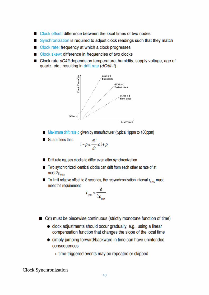
• C(t)=a*t+b
• a is a clock drift (rate)
• B is an offset of the clock
• Perfect clock
• Rate = 1
• Offset = 0
Definition of time synchronization
• Let C(t) be a perfect clock
A clock Ci(t) is called correct at time t
If Ci(t)=C(t)
A clock Ct(t) is called accurate at time t
If dCi(t)/dt = dC(t)/dt = 1
Two clocks Ci(t) and Ck(t) are synchronized at time t
if Ci(t)=Ck(t)
Time synchronization
• Requires knowing both offset and drift
• Most widely used time synchronization protocol
• Hierarchical: C/S model
• Perfectly acceptable for most cases.
• Coarse grain synchronization
• Inefficient when fine grain synchronization is required
Why Synchronization in WSNs?

39
Why Time Synchronization in WSNs?
Clocks and the Synchronization Problem
Clock Parameters
40
Clock Synchronization

41
Synchronization Messages

42
Receiver-Receiver Synchronization
Lightweight Tree-Based Synchronization

43
44
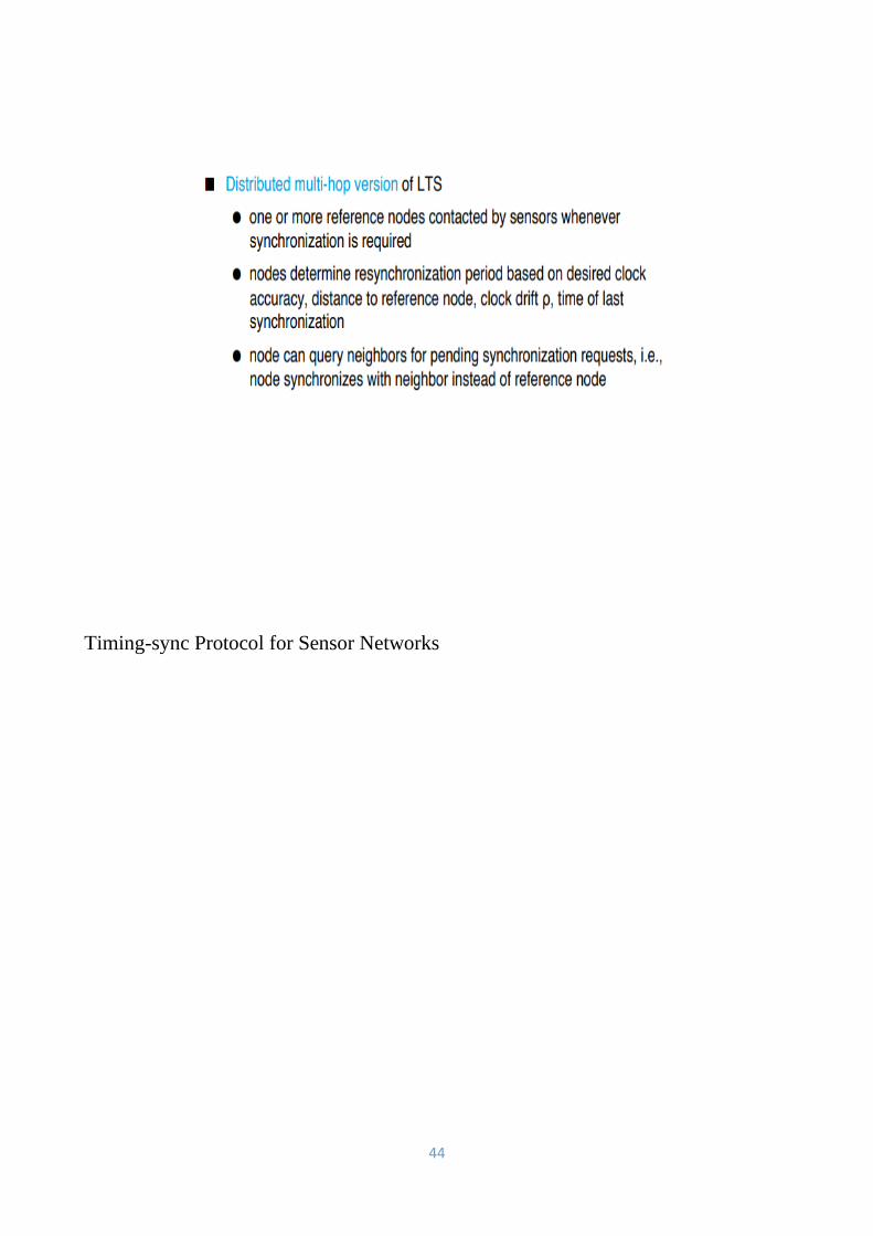
Timing-sync Protocol for Sensor Networks
45
Timing-sync Protocol for Sensor Networks
Timing-sync Protocol for Sensor Networks (TPSN) that aims at providing network-wide time
synchronization in a sensor network.
46
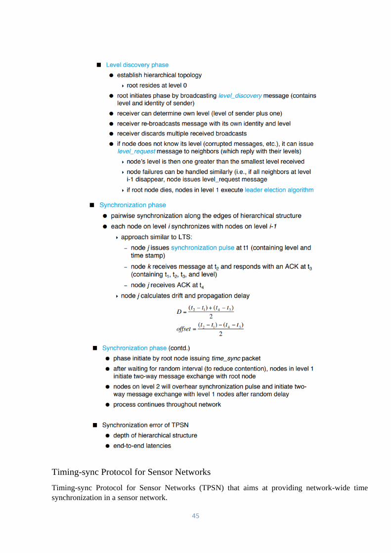
1. Level Discovery Phase
This phase of the algorithm occurs at the onset, when the network is deployed. The root node is
assigned a level 0 and itinitiates this phase by broadcasting a level_discovery packet. The
level_discovery packet contains the identity and the level of the sender. The immediate neighbors of
the root node receive this packet and assign themselves a level, one greater than the level they have
received i.e., level 1. After establishing their own level, they broadcast a new level_discovery packet
containing their own level. This process is continued and eventually every node in the network is
assigned a level. On being assigned a level, a node neglects any such future packets. This makes sure
that no flooding congestion takes place in this phase. Thus a hierarchical structure is created with
only one node, root node, at level 0. A node might not receive any level_discovery packets owing to
MAC layer collisions.
2. Synchronization Phase
n this phase, pair wise synchronization is performed along the edges of the hierarchical structure
established in the earlier phase.

47
SCHOOL OF COMPUTING
DEPARTMENT OF COMPUTER SCIENCE AND ENGINEERING
Unit- III- WIRELESS SENSOR NETWORKS-SCSA5202
48
Unit III
NODE LOCALIZATION AND DATA GATHERING
Node Localization: Absolute and Relative Localization-Triangulation-Multi-Hop Localization and
Error Analysis-Anchoring - Geographic Localization-Target Tracking - Localization and Identity
Management-Walking GPS-Range Free Solutions. Data Gathering - Tree Construction Algorithms and
Analysis - Asymptotic Capacity- Lifetime Optimization Formulations- Storage and Retrieval.
Deployment & Configuration - Sensor deployment, scheduling and coverage issues-Self configuration
and topology contro
Node Localization
Awareness of location is one of the important and critical issue and challenge in wireless sensor network.
Knowledge of Location among the participating nodes is one of the crucial requirements in designing of
solutions for various issues related to Wireless sensor networks. Wireless sensor networks are being used in
environmental applications to perform the number of task such as environment monitoring, disaster relief,
target tracking, defences and many more. In many such tasks, node localization is inherently one of the system
parameters. Node localization is required to report the origin of events, assist group querying of sensors,
routing and to answer questions on the network coverage. So, one of the fundamental challenges in wireless
sensor network is node localization.
PARAMETERS FOR LOCALIZATION
Accuracy: Accuracy is very important in the localization of wireless sensor network. Higher accuracy is
typically required in military installations, such as sensor network deployed for intrusion detection. However,
for commercial networks which may use localization to send advertisements from neighboring shops, the
required accuracy may not be lower. Cost: Cost is a very challenging issue in the localization of wireless
sensor network. There are very few algorithms which give low cost but those algorithms don’t give the high
rate of accuracy. Power: Power is necessary for computation purpose. Power play a major role in wireless
sensor network as each sensor device has limited power. Power supplied by battery. Static Nodes: All static
sensor nodes are homogeneous in nature. This means that, all the nodes have identical sensing ability,
computational ability, and the ability to communicate. We also assume that, the initial battery powers of the
nodes are identical at deployment. Mobile Nodes: It is assumed that a few number of GPS enabled mobile
nodes are part of the sensor network. These nodes are homogeneous in nature. But, are assumed to have more
battery power as compared to the static nodes and do not drain out completely during the localization process.
The communication range of mobile sensor nodes are assumed not to change drastically during the entire
localization algorithm runtime and also not to change significantly within the reception of four beacon
messages by a particular static node
Localization can be roughly divided into two categories: range-based and range-free. Range-based approach
uses absolute distance estimate or angle estimate, meaning that a node in a network can measure the distances
from itself to the beacons
In contrast, range-free approach means that it is impossible for a node to measure the direct distances from
itself to beacons. Only through connectivity and proximity, a node can estimate its regions or areas where it
49
stays. Range-based approach is precise while range-free method is often inaccurate. Range-based localization
can also divided into another two categories. One is distance estimation by one-hop; another is by multi-hop,
meaning that a node in the network can not directly communicate with beacons. Localization in WSN is a
multi-hop approach because a node may not communicate directly with beacons. Only through multi-hop
routing, can a node send or receive messages to or from beacons.
In terms of computation, the WSN localization algorithms can be classified into centralized and distributed
schemes. Further each category divided in to corresponding methods to solve localization problem. In the
centralized scheme, sensor nodes send control messages to a central node whose location is known. The central
node then computes the location of every sensor node and informs the nodes of their locations. In the
distributed scheme, each sensor node determines its own location independently.
Distributed Localization:
If each node collects partial data and executes the algorithm then localization algorithm is distributed. Beacon-
based distributed algorithms: Categorized into three parts: Diffusion: In diffusion the most likely position of
the node is at the centroid of its neighboring known nodes. APIT requires a high ratio of beacons to nodes
and longer range beacons to get a good position estimate. For low beacon density this scheme will not give
accurate results. Bounding box: Bounding box forms a bounding region for each node and then tries to refine
their positions. The collaborative multilateration enables sensor nodes to accurately estimate their locations
by using known beacon locations that are several hops away and distance measurements to neighboring nodes.
At the same time it increases the computational cost also. Gradient: Error in hop count distance matrices in
the presence of an obstacle. Relaxation-based distributed algorithms: The limitation of this approach is that
the algorithm is susceptible to local minima Coordinate system stitching based distributed algorithms: The
advantage of this approach is that no global resources or communications are needed. The disadvantage is that
convergence may take some time and that nodes with high mobility may be hard to cover. Hybrid localization
algorithms: The limitation of this scheme is that it does not perform well when there are only few anchors.
SHARP gives poor performance for anisotropic network. Interferometric ranging based localization:
Localization using this scheme requires considerably larger set of measurement which limits their solution to
smaller network
Centralized Localization: If an algorithm collects localization related data from one station and execute it
from the same station then it is called centralized. In centralized model the problem is that if computing server
fails due to some problem then entire processing goes down. Scalability is another problem when we consider
the centralized model for computation of our data. For security reasons this approach is also not best.
Localize node based on Simulated Annealing:
This algorithm does not propagate error in localization. The proposed flip ambiguity mitigation method is
based on neighborhood information of nodes and it works well in a sensor network with medium to high node
density. However when the node density is low, it is possible that a node is flipped and still maintains the
correct neighborhood. In this situation, the proposed algorithm fails to identify the flipped node. A RSSI-
based centralized localization technique: The advantage of this scheme is that it is a practical, self organizing
scheme that allows addressing any outdoor environments.The limitation of this scheme is that the scheme is
power consuming because it requires extensive generation and need to forward much information to the central
unit.
50
CUREENT ASPECTS IN LOCALIZTION
Resource constraints: Nodes must be cheap to fabricate, and trivially easy to deploy. Nodes must be cheap,
since fifty cents of additional cost per node translates to $500 for a one thousand node network. Deployment
must be easy as well: thirty seconds of handling time per node to prepare for localization translates to over
eight man-hours of work to deploy a 1000 node network. That means designers must actively work to
minimize the power cost, hardware cost and deployment cost of their localization algorithms. Node density:
.Many localization algorithms are sensitive to node density.
For instance, hop count based schemes generally require high node density so that the hop count
approximation for distance is accurate. Similarly, algorithms that depend on beacon nodes fail when the
beacon density is not high enough in a particular region. Thus, when designing or analysing an algorithm, it
is important to notice the algorithm’s implicit density assumptions, since high node density can sometimes be
expensive if not totally infeasible. Environmental obstacles and terrain irregularities: Environmental obstacles
and terrain irregularities can also wreak havoc on localization.
Large rocks can occlude line of sight, preventing TDoA ranging, or interfere with radios, introducing error
into RSSI ranges and producing incorrect hop count ranges. Indoors, natural features like walls can impede
measurements as well. All of these issues are likely to come up in real deployments, so localization systems
should be able to cope. Security: Security is the main issue in localization as the data is transferred from
beacon node to anchor node then any of mobile beacons which is a virus or not secure acting as original mobile
beacons transmit false messages due to this an error will occur which is harmful for our computation. Non
convex topologies: Border nodes are a problem because less information is available about them and that
information is of lower quality. This problem is exacerbated when a sensor network has a non-convex shape:
Sensors outside the main convex body of the network can often prove unlocalizable. Even when locations can
be found, the results tend to feature disproportionate error.
Global position
Global Positioning System or GPS (longitudes, latitudes)
Universal Transverse Mercator or UTM (zones and latitude bands) Relative position
based on arbitrary coordinate systems and reference frames distances between sensors (no relationship to
global coordinates) Accuracy versus precision
GPS: true within 10m for 90% of all measurements accuracy: 10m (“how close is the reading to the
ground truth?”) precision: 90% (“how consistent are the readings?”)

51
Example of range-based localization Uses the geometric properties of triangles to estimate location Relies
on angle (bearing) measurements Minimum of two bearing lines (and the locations of anchor nodes or the
distance between them) are needed for two-dimensional space
Triangulation Triangulation ‰ Lateration Lateration: use multiple distance : use multiple distance
measurements between measurements between known points known points ‰ Angulation Angulation:
measures angle or bearing relative to points : measures angle or bearing relative to points with known with
known separation
Geographic Distributed Localization
Localization schemes are classified as anchor based or anchor free, centralized or distributed, GPS based or
GPS free, fine grained or coarse grained, stationary or mobile sensor nodes, and range based or range free.
4.1. Anchor Based and Anchor Free
In anchor-based mechanisms, the positions of few nodes are known. Unlocalized nodes are localized by
these known nodes positions. Accuracy is highly depending on the number of anchor nodes. Anchor-free
algorithms estimate relative positions of nodes instead of computing absolute node positions
4.2. Centralized and Distributed
In centralized schemes, all information is passed to one central point or node which is usually called “sink
node or base station”. Sink node computes position of nodes and forwards information to respected nodes.
Computation cost of centralized based algorithm is decreased, and it takes less energy as compared with
computation at individual node. In distributed schemes, sensors calculate and estimate their positions
individually and directly communicate with anchor nodes. There is no clustering in distributed schemes,
and every node estimates its own position
4.3. GPS Based and GPS Free
GPS-based schemes are very costly because GPS receiver has to be put on every node. Localization
accuracy is very high as well. GPS-free algorithms do not use GPS, and they calculate the distance between
the nodes relative to local network and are less costly as compared with GPS-based schemes . Some nodes
need to be localized through GPS which are called anchor or beacon nodes that initiate the localization
process .
4.4. Coarse Grained and Fine Grained
Fine-grained localization schemes result when localization methods use features of received signal
strength, while coarse-grained localization schemes result without using received signal strength.

52
4.5. Stationary and Mobile Sensor Nodes
Localization algorithms are also designed according to field of sensor nodes in which they are deployed.
Some nodes are static in nature and are fixed at one place, and the majority applications use static nodes.
That is why many localization algorithms are designed for static nodes. Few applications use mobile sensor
nodes, for which few mechanisms are designed
Range-Free Methods
Range-free methods are distance vector (DV) hop, hop terrain, centroid system, APIT, and gradient
algorithm. Range-free methods use radio connectivity to communicate between nodes to infer their
location. In range-free schemes, distance measurement, angle of arrival, and special hardware are not used
DV Hop
DV hop estimates range between nodes using hop count. At least three anchor nodes broadcast coordinates
with hop count across the network. The information propagates across the network from neighbor to
neighbor node. When neighbor node receives such information, hop count is incremented by one . In this
way, unlocalized node can find number of hops away from anchor node. All anchor nodes calculate shortest
path from other nodes, and unlocalized nodes also calculate shortest path from all anchor nodes]. Average
hop distance formula is calculated as follows: distance between two nodes/number of hops.
Unknown nodes use triangulation method to estimate their positions from three or more anchor nodes
using hop count to measure shortest distance.
Hop Terrain
Hop terrain is similar to DV hop method in finding the distance between anchor node and unlocalized node.
There are two parts in the method. In the first part, unlocalized node estimates its position from anchor
node by using average hop distance formula which is distance between two nodes/total number
ofhops. This is initial position estimation. After initial position estimation, the second part executes, in
which initial estimated position is broadcast to neighbor nodes. Neighbor nodes receive this information
with distance information. A node refines its position until final position is met by using least square
method
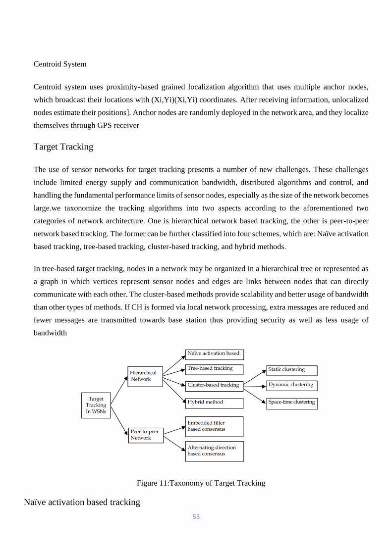
53
Centroid System
Centroid system uses proximity-based grained localization algorithm that uses multiple anchor nodes,
which broadcast their locations with (Xi,Yi)(Xi,Yi) coordinates. After receiving information, unlocalized
nodes estimate their positions]. Anchor nodes are randomly deployed in the network area, and they localize
themselves through GPS receiver
Target Tracking
The use of sensor networks for target tracking presents a number of new challenges. These challenges
include limited energy supply and communication bandwidth, distributed algorithms and control, and
handling the fundamental performance limits of sensor nodes, especially as the size of the network becomes
large.we taxonomize the tracking algorithms into two aspects according to the aforementioned two
categories of network architecture. One is hierarchical network based tracking, the other is peer-to-peer
network based tracking. The former can be further classified into four schemes, which are: Naïve activation
based tracking, tree-based tracking, cluster-based tracking, and hybrid methods.
In tree-based target tracking, nodes in a network may be organized in a hierarchical tree or represented as
a graph in which vertices represent sensor nodes and edges are links between nodes that can directly
communicate with each other. The cluster-based methods provide scalability and better usage of bandwidth
than other types of methods. If CH is formed via local network processing, extra messages are reduced and
fewer messages are transmitted towards base station thus providing security as well as less usage of
bandwidth
Figure 11:Taxonomy of Target Tracking
Naïve activation based tracking

54
Naïve activation (or direct communication) based tracking scheme is the simplest approach, for which all
nodes are in tracking mode all the time. Each node sends the local measurement to the sink node or base
station. Then the base station estimates and predicts the target state according to the received local
measurements. Since it offers the best tracking results, it is a useful baseline for comparison. However, this
strategy offers the worst energy efficiency and it inflects heavy communication and computation burden on
the base station of sink node. This makes the naïve approach not robust against base station failure especially
for the case of link failure and channel congestion.
Cluster-based tracking
To facilitate collaborative data processing in target tracking-centric sensor networks, the cluster architecture
is usually used in which sensors are organized into clusters, with each cluster consisting of a CH and several
slave nodes (members). Hierarchical (clustering) techniques can aid in reducing useful energy consumption
.). Clustering is particularly useful for applications that require scalability to hundreds or thousands of nodes.
Scalability in this context implies the need for load balancing and efficient resource utilization. Clustering can
be extremely effective in one-to-many, many-toone, one-to-any, or one-to-all (broadcast) communication. For
example, in many-to-one communication, clustering can support data fusion and reduce communication
interference
Tracking methods for peer-to-peer networks
It can guarantee that sensors obtain the desired estimates and rely only on singlehop communications between
neighbouring nodes, the limitations mentioned above are not encountered in peer-to-peer WSN based target
tracking systems.
DATA GATHERING IN WSN
Data gathering is recognized as one of the basic distributed data processing procedures in wireless sensor
networks for saving energy and reducing medium access layer contention.. A common function of sensor
networks in which the information are sampled at sensor nodes and are transported to central base stations for
further processing and analysis is called data gathering .The time sensitive data needs to be transmitted back
to the station in a near real time fashion for many data gathering applications such as object tracking and
intrusion detection. The applications like acoustic sensor networks, underwater or ocean sensor networks and
environmental monitoring do not need realtime data transmission and access. It can be used in scientific
applications by domain scientists to collect scientific data for further analysis The three major stages of data
collection are namely the deployment stage, the control message dissemination stage and the data delivery
stage .The issues regarding the deployment of the network is in the sensing field is addressed by the
deployment stage. The network setup/management and/or collection command messages are disseminated
from the base station to all sensor nodes in the control message dissemination stage. Here the challenge is to
disseminate messages to all the sensor nodes with small transmission costs and low latencies. The main task
of the sensor data collection is fulfilled by the data delivery stage
Importance of Data Gathering
Data gathering mechanism performs in-network aggregation of data which is needed for energy efficient
information flow. Data gathering protocols can reduce the communication cost, thereby extending the lifetime
of sensor networks
55
The inherent redundancy in raw data collected from the sensors can often be eliminated by in-network data
gathering. Data gathering can reduce the number of data packets transmitted and the data conflict thus raises
the data accuracy and data collection efficiency through dealing with the redundant data in network
Topology control
It is applied to deliberately restrict the set of nodes that are considered neighbors of a given node. This can
be done by controlling transmission power, by introducing hierarchies in the network and signaling out some
nodes to take over certain coordination tasks, or by simply turning off some nodes for a certain time
Aspects of topology-control algorithms
Connectivity Topology control should not disconnect a connected graph G. In other words, if there is a
(multihop) path in G between two nodes u and v, there should also be some such path in T (clearly, it does not
have to be the same path). Stretch factors Removing links from a graph will likely increase the length of a
path between any two nodes u and v.
Graph metrics The intuitive examples above already indicated the importance of a small number of edges in
T and a low maximum degree (number of neighbors) for each node.
Throughput The reduced network topology should be able to sustain a comparable amount of traffic as the
original network (this can be important even in wireless sensor networks with low average traffic, in particular,
in case of event showers). One metric to capture this aspect is throughput competitiveness (the largest φ ≤ 1
such that, given a set of flows from node si to node di with rate ri that are routable in G, the set with rates φri
can be routed in T
Robustness to mobility When neighborhood relationships change in the original graph G (for example,
because nodes move around or the radio channel characteristics change), some other nodes might have to
change their topology information (for example, to reactivate links). Clearly, a robust topology should only
require a small amount of such adaptations and avoid having the effects of a reorganization of a local node
movement ripple through the entire network.
Algorithm overhead It almost goes without saying that the overhead imposed by the algorithm itself should
be small (low number of additional messages, low computational overhead).
Sensor coverage
Sensor coverage is important while evaluating the effectiveness of a wireless sensor network. A lower
coverage level (simple coverage) is enough for environmental or habitat monitoring or applications like home
security .Higher degree of coverage (k-coverage) will be required for some applications like target tracking to
track the targets accurately or if sensors work in a hostile environment such as battle fields or chemically
polluted areas More reliable results are produced for higher degree of coverage which requires multiple sensor
nodes to monitor the region/targets. In some cases, for the same application, the coverage requirement may
vary. For example, for forest fire detections, the coverage level may be low in rainy seasons, but high in dry
seasons An example of Q-coverage is a video surveillance system deployed for monitoring hostile territorial
area where some sensitive targets like a nuclear plant may need more sensors cooperate to ensure source
redundancy for precise data Both sensor deployment and scheduling are important to ensure prolonged
network lifetime. Traditionally, the problems of sensor placement and scheduling have been considered

56
separately from each other. A balanced performance is crucial for most applications Different sensor
deployment strategies can cause very different network topology, and thus different degrees of sensor
redundancy A good sensor deployment with sufficient number of sensors which ensures a certain degree of
redundancy in coverage so that sensors can rotate between active and sleep modes is required to balance the
workload of sensors
Sensor Deployment 1) Sensor Deployment to Achieve 1-Coverage: Given a set of n targets T = {T1, T2,...,
Tn} located in u×v region and m sensor nodes S = {S1, S2,..., Sm}, place the nodes such that each target is
monitored by at least one sensor node and the network lifetime is maximum. The objective is to maximize U
such that each target is monitored by at least one sensor node. 2) Sensor Deployment to Achieve k-Coverage:
Given a set of n targets T = {T1, T2,..., Tn} located in u × v region and m sensor nodes S = {S1, S2,..., Sm},
place the nodes such that each target is monitored by at least k-sensor nodes and to maximize U. 3) Sensor
Deployment to Achieve Q-Coverage: Given a set of n targets T = {T1, T2,..., Tn} located in u×v region and
m sensor nodes S = {S1, S2,..., Sm}, place the nodes such that each target Tj , 1 ≤ j ≤ n, is covered by at least
q j sensor nodes and to maximize U
Sensor Deployment Since the upper bound of network lifetime can be computed, we have to find the
deployment locations such that the network lifetime is maximum. First we use a heuristic to compute the
deployment locations and then we use ABC and PSO algorithms to compute the locations. 1) A Heuristic for
Sensor Deployment: Here , a heuristic for sensor deployment Initially, place the sensor nodes randomly. If
any sensor node is idle (without monitoring any target), the node is moved to the least monitored targets’
location. This is to ensure that all sensor nodes play their part in monitoring the targets. The sensor nodes are
then sorted based on the number of targets it cover. The sensor node is placed at the middle of all the targets
it cover. The next nearest target is identified and the sensor node is placed at the middle of all these targets. If
it can cover this new target along with targets it was already monitoring, allow this move, else discard the
move. This is done till the sensor node cannot cover any new target. At the end, upper bound is computed.
The drawback of this approach is that it depends on the initial position of the sensor nodes. Though it may
perform well for dense deployments, consistency cannot always be guaranteed
ABC Based Sensor Deployment:
Artificial Bee Colony (ABC) Algorithm is an optimization algorithm based on the intelligent behavior of
honey bee swarm. The colony of bees contains three groups: employed bees, onlookers and scouts.The
employed bee takes a load of nectar from the source and returns to the hive and unloads the nectar to a food
store. After unloading the food, the bee performs a special form of dance called waggle dance which contains
information about the direction in which the food will be found, its distance from the hive and its quality
rating. Since information about all the current rich sources is available to an onlooker on the dance floor, an
onlooker bee probably could watch numerous dances and choose to employ itself at the most qualitative
source. There is a greater probability of onlookers choosing more qualitative sources since more information
is circulating about the more qualitative sources. Employed foragers share their information with a probability,
which is proportional to the quality of the food source. Hence, the recruitment is proportional to quality of a
food source Exploitation is carried out by employed bees and onlookers, while exploration is carried out by
scouts.
Sensor Deployment 1) Random Deployment: In random deployment, there is more chance of targets
being not detected or targets not being covered with the required level of coverage. However, this may not
hold true with dense deployment of nodes. But there is another possibility of some targets being monitored by
many sensor nodes, and some by a few sensor nodes. This difference in the number of sensor nodes monitoring

57
each target will affect the network lifetime. The sensor nodes may be positioned in a better way so as to avoid
this variation. This will yield better lifetime. Though random deployment has these drawbacks, there are
applications where random deployment is the only feasible strategy.
Heuristic: The heuristic could consistently achieve better results compared to random deployment when
the network size is increased

1
SCHOOL OF COMPUTING
DEPARTMENT OF COMPUTER SCIENCE AND ENGINEERING
SCSA5202-WIRELESS SENSOR NETWORKS
Unit- I- WIRELESS SENSOR NETWORKS-SCSA5202
2
UNIT 4
ROUTING AND DISTRIBUTED COMPUTATION
Routing: Agent-Based Routing -Random Walk-Trace Routing Data Centric-Hierarchical -
Location-Based – Energy Efficient-Routing Querying-Data Collection and Processing-
Collaborative Information Processing And Group Connectivity.
ROUTING:
Routing in WSNs can be divided into flat-based routing, hierarchical-based routing, and location-
based routing depending on the network structure. In flat-based routing, all nodes are typically
assigned equal roles or functionality. In hierarchical-based routing, however, nodes will play
different roles in the network. In location-based routing, sensor nodes’ positions are exploited to
route data in the network. A routing protocol is considered adaptive if certain system parameters
can be controlled in order to adapt to the current network conditions and available energy levels.
Furthermore, these protocols can be classified into multipath-based, query-based, negotiation-
based, QoS-based, or coherent-based routing techniques depending on the protocol operation.
In addition to the above, routing protocols can be classified into three categories, namely,
proactive, reactive, and hybrid protocols depending on how the source finds a route to the
destination. In proactive protocols, all routes are computed before they are really needed, while in
reactive protocols, routes are computed on demand. Hybrid protocols use a combination of these
two ideas. When sensor nodes are static, it is preferable to have table driven routing protocols
rather than using reactive protocols. A significant amount of energy is used in route discovery and
setup of reactive protocols. Another class of routing protocol is called the cooperative routing
protocols.
AGENT BASED ROUTING:
➢ Agent-based routing approach is One of the main objectives of WSNs is to report back the
events of user’s interest. The user interests are injected into a network by the Sink. Sink is
a special node that acts like a server. The node that can identify the user requested interest
is called source node. The source nodes report back the events to the sink. The WSN
consists of uncountable nodes deployed with limited amount of banked energy,
replenishment of which is a tedious task. This banked energy marks the life time on these
nodes.
➢ Utilizing the energy of the nodes equitably and intelligently increases the life time of WSN
into many folds. Hence, a scalable and intelligent routing approach is required. Towards
this end, we propose AbR system that is scalable and intelligent enough to avoid
continuously using and burning nodes energy along the shortest path to source node.
Therefore, nodes along the shortest path will be provided a fair chance to rest by
distributing their duty cycles to neighboring nodes.

3
➢ This may lead to exploration of energy expensive path toward source node, however in the
long run network connectivity is maintained for longer period of time and abrupt node
depletion is not witnessed. The sudden breakdown of aggressively used nodes in the
optimal path creates connectivity holes in the network. This leads to the early segmentation
of network with price payoff as inefficient and costly routing at later stage.
➢ To cut down on such sumptuous price payoff, developed two types of agent: stationary
agent (SA) and mobile agent (MA).
Figure 1: Agent Based Routing
➢ Every node on the sensor network is equipped with stationary agent. The role of SA is to
acquire knowledge about its environment. The mobile agent is created and injected into the
network by sink (SI). The MA benefits from the knowledge acquired by SA to select its
next hop towards source node (SO), to distribute interest or processing code or report data
to SI.
RANDOM WALK ROUTING:
The objective of random walks-based routing technique is to achieve load balancing in a statistical
sense and by making use of multi-path routing in WSNs. This technique considers only large-scale
networks where nodes have very limited mobility. In this protocol, it is assumed that sensor nodes
can be turned on or off at random times. Further, each node has a unique identifier but no location
information is needed. Nodes were arranged such that each node falls exactly on one crossing point
of a regular grid on a plane, but the topology can be irregular. To find a route from a source to its
destination, the location information or lattice coordination is obtained by computing distances
between nodes using the distributed asynchronous version of the well-known Bellman-Ford
algorithm.
Random walk- based routing is a probabilistic protocol in which each node selects randomly from
its neighbor’s nodes to forward the data packet. The path thus formed is a random walk (RW). RW
based routing protocol is often proposed for very small devices, in large and dynamic networks
due to being extremely simple to implement, requiring small memory footprints, and not requiring
topology information of the network and load balancing property of the RW. On the other hand,

4
reactive (on-demand) routing protocols are also considered to be useful in resource constrained
and dynamic WSNs.
However due to their inherent properties, increasing density of nodes badly affects performance
of such protocols in terms of scalability. Furthermore, high mobility of sensor nodes and enabling
low duty cycling make routing quite challenging. In such scenarios, random walk-based routing
has not been studied widely. In this paper, we have put before a Lightweight Random Walk based
Routing (LRWR) protocol in which each step follows a three messages exchange not only to
discover neighbors but also to randomly select and forward the packets to the selected neighbor.
We call this protocol lightweight since the number of messages required to achieve one step of
RW are bare minimum. We applied the LRWR protocol in WSN with IEEE 802.15.4 standard and
duty cycle enabled environments. By comparing its performance for low data rate with DYMO, a
widely used protocol for WSN, we find that LRWR protocol offers a better alternative for duty
cycle enabled mobile WSNs.
Figure 2: Random Walk
An intermediate node would select as the next hop the neighboring node that is closer to the
destination according to a computed probability. By carefully manipulating this probability, some
kind of load balancing can be obtained in the network. The routing algorithm is simple as nodes
are required to maintain little state information. Moreover, different routes are chosen at different
times even for the same pair of source and destination nodes. However, the main concern about
this protocol is that the topology of the network may not be practical.
HIERARCHICAL ROUTING:
Hierarchical or cluster-based routing, originally proposed in wireline networks, are well-known
techniques with special advantages related to scalability and efficient communication. As such,
the concept of hierarchical routing is also utilized to perform energy-efficient routing in WSNs. In

5
a hierarchical architecture, higher energy nodes can be used to process and send the information
while low energy nodes can be used to perform the sensing in the proximity of the target.
This means that creation of clusters and assigning special tasks to cluster heads can greatly
contribute to overall system scalability, lifetime, and energy efficiency. Hierarchical routing is an
efficient way to lower energy consumption within a cluster and by performing data aggregation
and fusion in order to decrease the number of transmitted messages to the BS.
Hierarchical routing is mainly two-layer routing where one layer is used to select cluster heads and
the other layer is used for routing. However, most techniques in this category are not about routing,
rather on” who and when to send or process/aggregate” the information, channel allocation etc.,
which can be orthogonal to the multihop routing function.
Figure 3: Hierarchical Routing
• LEACH protocol: Low Energy Adaptive Clustering Hierarchy (LEACH). LEACH is a
cluster-based protocol, which includes distributed cluster formation. LEACH randomly selects a
few sensor nodes as cluster heads (CHs) and rotate this role to evenly distribute the energy load
among the sensors in the network. In LEACH, the cluster head (CH) nodes compress data arriving
from nodes that belong to the respective cluster, and send an aggregated packet to the base station
6
in order to reduce the amount of information that must be transmitted to the base station. LEACH
uses a TDMA/CDMA MAC to reduce inter-cluster and intra-cluster collisions. However, data
collection is centralized and is performed periodically. Therefore, this protocol is most appropriate
when there is a need for constant monitoring by the sensor network. A user may not need all the
data immediately. Hence, periodic data transmissions are unnecessary which may drain the limited
energy of the sensor nodes. After a given interval of time, a randomized rotation of the role of the
CH is conducted so that uniform energy dissipation in the sensor network is obtained.
The operation of LEACH is separated into two phases, the setup phase and the steady state phase.
➢ In the setup phase, the clusters are organized and CHs are selected. In the steady state
phase, the actual data transfer to the base station takes place. The duration of the steady
state phase is longer than the duration of the setup phase in order to minimize overhead.
During the setup phase, a predetermined fraction of nodes, p, elect themselves as CHs as
follows. A sensor node chooses a random number, r, between 0 and 1. If this random
number is less than a threshold value, T(n), the node becomes a cluster-head for the current
round. The threshold value is calculated based on an equation that incorporates the desired
percentage to become a cluster-head, the current round, and the set of nodes that have not
been selected as a cluster-head in the last (1/P) rounds, denoted by G. It is given by:
T(n) = p / 1 − p(r mod (1/p)) if n ∈ G
where G is the set of nodes that are involved in the CH election. Each elected CH broadcast an
advertisement message to the rest of the nodes in the network that they are the new cluster-heads.
All the non-cluster head nodes, after receiving this advertisement, decide on the cluster to which
they want to belong to. This decision is based on the signal strength of the advertisement. The non
cluster-head nodes inform the appropriate cluster-heads that they will be a member of the cluster.
After receiving all the messages from the nodes that would like to be included in the cluster and
based on the number of nodes in the cluster, the cluster-head node creates a TDMA schedule and
assigns each node a time slot when it can transmit. This schedule is broadcast to all the nodes in
the cluster.
➢ During the steady state phase, the sensor nodes can begin sensing and transmitting data to
the cluster-heads. The cluster-head node, after receiving all the data, aggregates it before
sending it to the base-station. After a certain time, which is determined a priori, the network
goes back into the setup phase again and enters another round of selecting new CH. Each
cluster communicates using different CDMA codes to reduce interference from nodes
belonging to other clusters
• Power-Efficient Gathering in Sensor Information Systems (PEGASIS): an
enhancement over LEACH protocol was proposed. The protocol, called Power-Efficient Gathering
in Sensor Information Systems (PEGASIS), is a near optimal chain-based protocol. The basic idea
of the protocol is that in order to extend network lifetime, nodes need only communicate with their
closest neighbors and they take turns in communicating with the base-station. When the round of
all nodes communicating with the base-station ends, a new round will start and so on. This reduces
7
the power required to transmit data per round as the power draining is spread uniformly over all
nodes. Hence, PEGASIS has two main objectives. First, increase the lifetime of each node by using
collaborative techniques and as a result the network lifetime will be increased. Second, allow only
local coordination between nodes that are close together so that the bandwidth consumed in
communication is reduced. Unlike LEACH, PEGASIS avoids cluster formation and uses only one
node in a chain to transmit to the BS instead of using multiple nodes.
To locate the closest neighbor node in PEGASIS, each node uses the signal strength to measure
the distance to all neighboring nodes and then adjust the signal strength so that only one node can
be heard. The chain in PEGASIS will consist of those nodes that are closest to each other and form
a path to the base-stationSuch performance gain is achieved through the elimination of the
overhead caused by dynamic cluster formation in LEACH and through decreasing the number of
transmissions and reception by using data aggregation.
Although the clustering overhead is avoided, PEGASIS still requires dynamic topology adjustment
since a sensor node needs to know about energy status of its neighbors in order to know where to
route its data. Such topology adjustment can introduce significant overhead especially for highly
utilized networks. Moreover, PEGASIS assumes that each sensor node can be able to communicate
with the BS directly. In practical cases, sensor nodes use multihop communication to reach the
base-station
• Threshold-sensitive Energy Efficient Protocols (TEEN and APTEEN): Two
hierarchical routing protocols called TEEN (Threshold-sensitive Energy Efficient sensor Network
protocol), and APTEEN (Adaptive Periodic Threshold-sensitive Energy Efficient sensor Network
protocol). These protocols were proposed for time-critical applications. In TEEN, sensor nodes
sense the medium continuously, but the data transmission is done less frequently. A cluster head
sensor sends its members a hard threshold, which is the threshold value of the sensed attribute and
a soft threshold, which is a small change in the value of the sensed attribute that triggers the node
to switch on its transmitter and transmit. Thus, the hard threshold tries to reduce the number of
transmissions by allowing the nodes to transmit only when the sensed attribute is in the range of
interest. The soft threshold further reduces the number of transmissions that might have otherwise
occurred when there is little or no change in the sensed attribute. A smaller value of the soft
threshold gives a more accurate picture of the network, at the expense of increased energy
consumption.
Thus, the user can control the trade-off between energy efficiency and data accuracy. When
cluster-heads are to change new values for the above parameters are broadcast. The main drawback
of this scheme is that, if the thresholds are not received, the nodes will never communicate, and
the user will not get any data from the network at all. The nodes sense their environment
continuously. The first time a parameter from the attribute set reaches its hard threshold value, the
node switches its transmitter on and sends the sensed data. The sensed value is stored in an internal
variable, called Sensed Value (SV). The nodes will transmit data in the current cluster period only
when the following conditions are true: (1) The current value of the sensed attribute is greater than
the hard threshold (2) The current value of the sensed attribute differs from SV by an amount equal
to or greater than the soft threshold.
8
In APTEEN, the cluster-heads broadcasts the following parameters
1. Attributes (A): this is a set of physical parameters which the user is interested in obtaining
information about.
2. Thresholds: this parameter consists of the Hard Threshold (HT) and the Soft Threshold (ST).
3. Schedule: this is a TDMA schedule, assigning a slot to each node.
4. Count Time (CT): it is the maximum time period between two successive reports sent by a node.
• Small Minimum Energy Communication Network (MECN): an energy-efficient
subnetwork, namely the minimum energy communication network (MECN) for a certain sensor
network by utilizing low power GPS. MECN identifies a relay region for every node. The relay
region consists of nodes in a surrounding area where transmitting through those nodes is more
energy efficient than direct transmission. The main idea of MECN is to find a sub-network, which
will have a smaller number of nodes and require less power for transmission between any two
particular nodes. In this way, global minimum power paths are found without considering all the
nodes in the network. This is performed using a localized search for each node considering its
relay region. MECN is self-reconfiguring and thus can dynamically adapt to nodes failure or the
deployment of new sensors.
The small minimum energy communication network (SMECN) is an extension to MECN. In
MECN, it is assumed that every node can transmit to every other node, which is not possible every
time
• Self Organizing Protocol (SOP): a self-organizing protocol and an application taxonomy
that was used to build architecture used to support heterogeneous sensors. Furthermore, these
sensors can be mobile or stationary. Some sensors probe the environment and forward the data to
a designated set of nodes that act as routers. Router nodes are stationary and form the backbone
for communication.
In this approach, sensor nodes can be addressed individually in the routing architecture, and hence
it is suitable for applications where communication to a particular node is required. Furthermore,
this algorithm incurs a small cost for maintaining routing tables and keeping a balanced routing
hierarchy. It was also found that the energy consumed for broadcasting a message is less than that
consumed in the SPIN protocol. This protocol, however, is not an on-demand protocols especially
in the organization phase of algorithm. Therefore, introducing extra overhead. Another issue is
related to the formation of hierarchy. It could happen that there are many cuts in the network, and
hence the probability of applying reorganization phase increases, which will be an expensive
operation.
• Sensor Aggregates Routing: A sensor aggregate comprises those nodes in a network that
satisfy a grouping predicate for a collaborative processing task. The parameters of the predicate
depend on the task and its resource requirements. Sensors in a sensor field is divided into clusters
according to their sensed signal strength, so that there is only one peak per cluster. Then, local
cluster leaders are elected.

9
One peak may represent one target, multiple targets, or no target in case the peak is generated by
noise sources. To elect a leader, information exchanges between neighboring sensors are
necessary. If a sensor, after exchanging packets with all its one-hop neighbors, finds that it is higher
than all its one-hop neighbors on the signal field landscape, it declares itself a leader. This leader-
based tracking algorithm assumes the unique leader knows the geographical region of the
collaboration.
• Hierarchical Power-aware Routing (HPAR): a hierarchical power-aware routing
protocol divides the network into groups of sensors. Each group of sensors in geographic proximity
are clustered together as a zone and each zone is treated as an entity. To perform routing, each
zone is allowed to decide how it will route a message hierarchically across the other zones such
that the battery lives of the nodes in the system are maximized. Message are routed along the path
which has the maximum over all the minimum of the remaining power, called the max-min path.
The motivation is that using nodes with high residual power may be expensive as compared to the
path with the minimal power consumption. An approximation algorithm, called the max-min
algorithm, First, the algorithm finds the path with the least power consumption (Pmin) by using
the Dijkstra algorithm. Second, the algorithm finds a path that maximizes the minimal residual
power in the network.
DATA CENTRIC ROUTING:
Data-centric protocols differ from traditional address centric protocols in the manner that the data
is sent from source sensors to the sink. In address-centric protocols, each source sensor that has
the appropriate data responds by sending its data to the sink independently of all other sensors.
However, in datacentric protocols, when the source sensors send their data to the sink, intermediate
sensors can perform some form of aggregation on the data originating from multiple source sensors
and send the aggregated data toward the sink. This process can result in energy savings because of
less transmission required to send the data from the sources to the sink. Following f the data-centric
routing protocols for WSNs.
A. Sensor Protocols for Information via Negotiation (SPIN): SPIN protocol was designed to
improve classic flooding protocols and overcome the problems they may cause, for example,
implosion and overlap. The SPIN protocols are resource aware and resource adaptive. The
sensors running the SPIN protocols are able to compute the energy consumption required to
compute, send, and receive data over the network. Thus, they can make informed decisions
for efficient use of their own resources. The SPIN protocols are based on two key mechanisms
namely negotiation and resource adaptation. SPIN uses meta-data as the descriptors of the data
that the sensors want to disseminate. The notion of meta-data avoids the occurrence of overlap
given sensors can name the interesting portion of the data they want to get. It may be noted
here that the size of the meta-data should definitely be less than that of the corresponding
sensor data. This allows the sensors to use their energy and bandwidth efficiently.
B. Directed Diffusion (DD): Direct diffusion is a data centric query based and application-
aware protocol where data aggregation is carried out at each node in the network. The nodes
will not advertise the sensed data until a request is made by the BS, and all the data generated
by sensor node is named by attribute-value pairs. The gradient specifies data rate and the
10
direction in which to send the events. The node which receives the events information from
the source attempts to find a matching entry in its interest cache. All sensor nodes in a directed-
diffusion-based network are application-aware, which enables diffusion to achieve energy
savings by selecting empirically good paths, and by caching and processing data in the
network. Caching can increase the efficiency, robustness, and scalability of coordination
between sensor nodes, which is the essence of the data diffusion paradigm.
C. Rumor Routing (RR): Rumor routing is another variation of Directed Diffusion and is
mainly intended for contexts in which geographic routing criteria are not applicable. Generally
Directed Diffusion floods the query to the entire network when there is no geographic criterion
to diffuse tasks. However, in some cases there is only a little amount of data requested from
the nodes and thus the use of flooding is unnecessary. An alternative approach is to flood the
events if number of events is small and number of queries is large. Rumor routing is between
event flooding and query flooding. The idea is to route the queries to the nodes that have
observed a particular event rather than flooding the entire network to retrieve information
about the occurring events. In order to flood events through the network, the rumor routing
algorithm employs long-lived packets, called agents. When a node detects an event, it adds
such event to its local table and generates an agent. Agents travel the network in order to
propagate information about local events to distant nodes. When a node generates a query for
an event, the nodes that know the route, can respond to the query by referring its event table.
Hence, the cost of flooding the whole network is avoided. Rumor routing maintains only one
path between source and destination as opposed to Directed Diffusion where data can be sent
through multiple paths at low rates.
D. COUGAR: A data-centric protocol that views the network as a huge distributed database
system. The main idea is to use declarative queries in order to abstract query processing from
the network layer functions such as selection of relevant sensors etc. and utilize in-network
data aggregation to save energy. The abstraction is supported through a new query layer
between the network and application layers. COUGAR proposes architecture for the sensor
database system where sensor nodes select a leader node to perform aggregation and transmit
the data to the gateway.
E. Active Query Forwarding in Sensor Networks (ACQUIRE): ACQUIRE is another data
centric querying mechanism used for querying named data. It provides superior query
optimization to answer specific types of queries, called one-shot complex queries for
replicated data. ACQUIRE query (i.e., interest for named data) consists of several sub queries
for which several simple responses are provided by several relevant sensors. Each sub-query
is answered based on the currently stored data at its relevant sensor. ACQUIRE allows a sensor
to inject an active query in a network following either a random or a specified trajectory until
the query gets answered by some sensors on the path using a localized update mechanism.
Unlike other query techniques, ACQUIRE allows the queries to inject a complex query into
the network to be forwarded stepwise through a sequence of sensors
F. DRUG: This protocol introduces a novel adaptive approach to find an optimal routing path
from source to sink when the sensor nodes are deployed randomly deployed in a restricted
service area with single sink. This also aggregates the data in intermediate node to reduce the
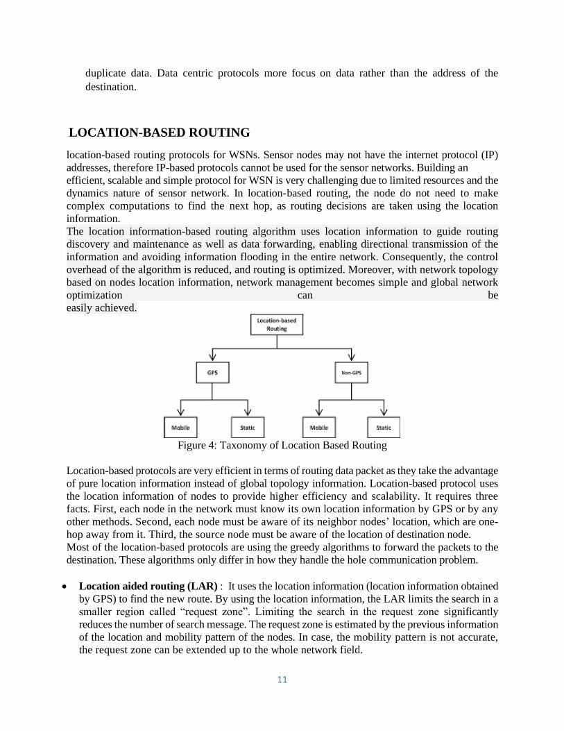
11
duplicate data. Data centric protocols more focus on data rather than the address of the
destination.
LOCATION-BASED ROUTING
location-based routing protocols for WSNs. Sensor nodes may not have the internet protocol (IP)
addresses, therefore IP-based protocols cannot be used for the sensor networks. Building an
efficient, scalable and simple protocol for WSN is very challenging due to limited resources and the
dynamics nature of sensor network. In location-based routing, the node do not need to make
complex computations to find the next hop, as routing decisions are taken using the location
information.
The location information-based routing algorithm uses location information to guide routing
discovery and maintenance as well as data forwarding, enabling directional transmission of the
information and avoiding information flooding in the entire network. Consequently, the control
overhead of the algorithm is reduced, and routing is optimized. Moreover, with network topology
based on nodes location information, network management becomes simple and global network
optimization can be
easily achieved.
Figure 4: Taxonomy of Location Based Routing
Location-based protocols are very efficient in terms of routing data packet as they take the advantage
of pure location information instead of global topology information. Location-based protocol uses
the location information of nodes to provide higher efficiency and scalability. It requires three
facts. First, each node in the network must know its own location information by GPS or by any
other methods. Second, each node must be aware of its neighbor nodes’ location, which are one-
hop away from it. Third, the source node must be aware of the location of destination node.
Most of the location-based protocols are using the greedy algorithms to forward the packets to the
destination. These algorithms only differ in how they handle the hole communication problem.
• Location aided routing (LAR) : It uses the location information (location information obtained
by GPS) to find the new route. By using the location information, the LAR limits the search in a
smaller region called “request zone”. Limiting the search in the request zone significantly
reduces the number of search message. The request zone is estimated by the previous information
of the location and mobility pattern of the nodes. In case, the mobility pattern is not accurate,
the request zone can be extended up to the whole network field.
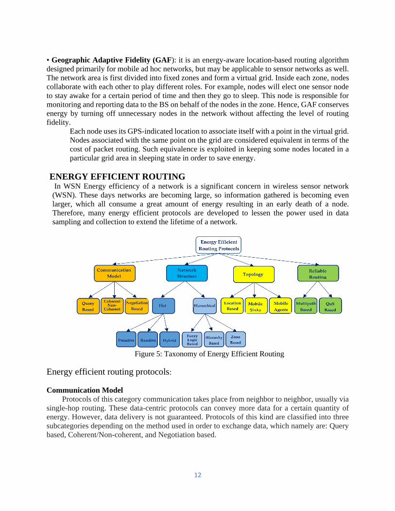
12
• Geographic Adaptive Fidelity (GAF): it is an energy-aware location-based routing algorithm
designed primarily for mobile ad hoc networks, but may be applicable to sensor networks as well.
The network area is first divided into fixed zones and form a virtual grid. Inside each zone, nodes
collaborate with each other to play different roles. For example, nodes will elect one sensor node
to stay awake for a certain period of time and then they go to sleep. This node is responsible for
monitoring and reporting data to the BS on behalf of the nodes in the zone. Hence, GAF conserves
energy by turning off unnecessary nodes in the network without affecting the level of routing
fidelity.
Each node uses its GPS-indicated location to associate itself with a point in the virtual grid.
Nodes associated with the same point on the grid are considered equivalent in terms of the
cost of packet routing. Such equivalence is exploited in keeping some nodes located in a
particular grid area in sleeping state in order to save energy.
ENERGY EFFICIENT ROUTING In WSN Energy efficiency of a network is a significant concern in wireless sensor network
(WSN). These days networks are becoming large, so information gathered is becoming even
larger, which all consume a great amount of energy resulting in an early death of a node.
Therefore, many energy efficient protocols are developed to lessen the power used in data
sampling and collection to extend the lifetime of a network.
Figure 5: Taxonomy of Energy Efficient Routing
Energy efficient routing protocols:
Communication Model
Protocols of this category communication takes place from neighbor to neighbor, usually via
single-hop routing. These data-centric protocols can convey more data for a certain quantity of
energy. However, data delivery is not guaranteed. Protocols of this kind are classified into three
subcategories depending on the method used in order to exchange data, which namely are: Query
based, Coherent/Non-coherent, and Negotiation based.
13
1.Query Based:
Protocols of this subcategory use queries in order to route data. Whenever a node needs new
data, it propagates a message (query) to ask for these data from the node that has them. Next, the
node which owns the data requested sends them to the node that has applied the query. In what
follows in this section, six typical examples of query based energy efficient routing protocols are
described.
Directed Diffusion (DD) is a protocol that uses a naming scheme for data packets. It saves
energy by diffusing data through the nodes and preventing unnecessary operations to run.DD uses
a list of attribute-value pairs, with which it defines interests as object name, transmission, or
geographic location. Interests are broadcasted from the BS to its neighbors and can be cached for
later use. Interest caching includes gradients. Gradient is a reply link, from the neighbor sent the
interest, which is described by data flow, duration, and expiring time generated from received
interests. The nodes can do in-network data aggregation that is modeled as a minimum Steiner
tree. Combining interests and gradients, multiple paths are generated between the BS and nodes,
with one path been chosen using reinforcement.
To achieve this, the BS resends the initial interest from the selected path, in smaller intervals,
resulting in reinforcement of the source node to send data more frequently. When a route failure
occurs, DD tries to create a new or an alternative path by reinitiating reinforcement to search for
new paths with lower casting ratios. The main advantages of DD are that node addressing
mechanisms are not needed and there is no need for global knowledge of network topology. In
addition, high energy efficiency is achieved.
COUGAR is a protocol that perceives the network as a distributed database system. It uses
declarative queries to replace the network layer functions of query processing, as the selection of
relevant nodes and utilizes in network data aggregation to save energy. To replace the network
layer functions, it imports an additional layer, called query layer, between network and application
layer. In COUGAR’s architecture, nodes select a leader node for data aggregation and transmission
to the BS. The main advantage of COUGAR is that it provides energy efficiency even with huge
number of active nodes.
Active Query Forwarding In Sensor Networks (Acquire) uses a data centric mechanism
for query sending and perceives the network as a distributed database, as COUGAR, which can
divide complex queries in many sub-queries. The BS transmits a query, which is forwarded from
every node that receives it. Upon query forwarding, nodes use their pre-cached information to
reply to the query partially, updating pre-cached information from neighbor nodes, when needed,
within a d hops distance. After the query is resolved, it can be sent back to the BS either from the
reverse path or the shortest path. ACQUIRE provides efficient queries with proper setting of look-
ahead parameter d. The traffic behaves like flooding when look-ahead parameter d is equal to
network size but when the parameter is significant small queries have to travel more. ACQUIRE
provides efficient querying when responses are collected from many nodes. However, if the look-
ahead parameter is too small, query travels more hops.
Energy aware routing is a data centric routing protocol that constantly uses non optimal
paths to maximize network lifetime. To pick one of these paths, it uses a probability function that
depends on energy consumption of each path. This approach takes into consideration network
lifetime as the only metric attribute. Instead of using the minimum energy path, it uses multiple
routes with a certain probability to maximize network lifetime.
The operation of the routing protocol has three phases:

14
(i) Setup phase: Localized flooding is performed to find all paths from source to
destination, calculate corresponding energy costs and create routing tables.
(ii) Data Communication phase: Based on the energy costs calculated, routing paths are chosen
probabilistically and data are sent from source to destination.
(iii) Routing maintenance phase: With the intermittent use of localized flooding, routing paths are
kept alive.
Gradient Based Routing (GBR) is a variant of Directed Diffusion. It combines the number
of hops with interests and creates link heights and gradients to improve data communication. When
an interest is diffused through the network, the number of hops is stored. Every node can find out
the minimum number of hops to the BS, called node’s height. A packet is transmitted through a
link with a high gradient. The algorithm uniformly balances traffic over the network, which helps
to balance nodes’ load and prolong network lifetime, using techniques as data aggregation and
traffic spread, as nodes act as relays for multiple paths. It uses three data spreading techniques:
(i) Stochastic design: the sender node picks one link in random in case there are two or
more hops with the same gradient.
(ii) Energy based design: when a node has energy below a specified threshold, it increases
its height to discourage other neighbors to transmit data.
(iii) Flow based design: flows from nodes that are part of other flows are prevented.
(iv)
Compared to DD, GBR has lower communication energy consumption
2.Coherent/Non-Coherent:
In this subcategory, nodes process collected data in the node level before they route them. In
Coherent protocols, a node applies minimum processing only on the data it captures. On the other
hand, in non-coherent routing protocols, nodes preprocess data they capture and send them to
nodes, called aggregators, which further process them. In what follows in this section, two typical
examples of this subcategory are described.
Single Winner Algorithm (SWE) an aggregator node, called Central Node (CN), to perform
complex computations, depending on energy reservoirs and computational power. There are
various message broadcasts before a CN can be elected. The first message is an announcement of
nomination of each node and, when another node receives the message, it compares those
candidates with itself. This comparison creates a second message broadcast, with the result of the
comparison being sent again for another comparison, until a CN is elected. During the message
broadcasts, better candidates create a minimum hop spanning tree, routed at the winning
candidates, covering eventually the entire network.
Multiple Winner Algorithm (MWE) is an extension of SWE to prevent extra energy and
computational overhead when multiple sources send data to CN. In MWE, each node keeps records
of best candidate nodes and a set of minimum energy paths to each source. Thus, both energy and
overhead are saved. Then, SWE is used to elect the best candidate for CN to aggregate data. Thus,
energy consumption is reduced and a set of minimum energy routes to each source is found.
However, long delays are caused and the scalability achieved is limited.
3.Negotiation Based
In this subcategory routing protocols, a source node exchanges data with their destination
after negotiating. These protocols name data based on a naming scheme and use these names to
advertise, negotiate and eventually reduce redundant data at destination. In what follows in this

15
section, SPIN family protocols, which are typical examples of this negotiation based energy
efficient routing, protocols are described.
Sensor Protocols for Information via Negotiation (SPIN) is a protocol that names the data
using high level descriptors or meta-data. Before data transmission takes place, meta-data are
exchanged among nodes via an advertisement mechanism. The meta-data format is no standard,
but it depends on the application. Every node upon receiving new data advertises packets to its
neighbors with advertisement messages (ADV). Interested neighbors, who do not have the data,
send a request message (REQ). Then, sending nodes send the actual data (DATA) to interested
nodes. This negotiation of meta-data not only solves the classic problems of Flooding, but also is
more energy efficient. In addition, metadata negotiation reduces in half redundant data and changes
in topology are localized.
SPIN Point to Point (SPIN-PP) is a variant of SPIN for communication between only two
nodes that use the same 3-way handshake SPIN algorithm. When new data are available at a node,
it sends ADV messages. Interested nodes send an REQ message back to the source, in order to
show their interest for these new data. Then, the source replies with a DATA message containing
the data. This algorithm is executed between two nodes, without any interference. In addition, as
it happens in SPIN too, SPIN-PP does not take into consideration energy constrains. In SPINN-PP
protocol, set-up simplicity is offered, and implosion is avoided. However, needless energy
consumption takes place while data delivery is not guaranteed.
SPIN-Energy Conservation (SPIN-EC) protocol uses the same algorithm of SPIN-PP but
adds a heuristic of energy conservation. To take into consideration energy constraints, SPIN-EC
uses an energy threshold. Nodes, whose residual energy is below this threshold, can receive ADV
or REQ messages, but they will not send REQ messages if they are interested or will not handle
DATA messages. SPIN-EC considers energy constraints and properly adapts its operation.
However, nodes even below the low energy threshold keep consuming energy because they are
still able to receive ADV and REQ messages.
SPIN for Broadcast Networks (SPIN-BC) is another variation of SPIN protocol that uses
one to many communications. The source sends the ADV message to all nodes in its range and
interested nodes wait for a predetermined time before they send an REQ message. In case they
receive an REQ message from another interested node, they cancel their REQ message to limit
unnecessary requests. The source, in the case that it receives the REQ message, broadcasts the
DATA message once, regardless of the number of REQ messages. SPIN-BC uses cheap one to
many communications. It also achieves good scalability and generally performs better than SPIN-
PP. However, there is a waiting time before sending the REQ message.
Network Structure
Protocols belonging to the network structure scheme are classified in two subcategories
according to whether the nodes are treated as equals or whether they are members of a hierarchy.
These subcategories are:
➢ Flat
In Flat subcategory, nodes are considered to be equal entities with unique global addresses.
Protocols of this type can be further classified into three different operational categories which
namely are: proactive protocols, reactive protocols, and hybrid protocols.
1. Proactive
16
The proactive protocols are constantly active waiting to sense anything with the result of a
quicker response and a greater energy consumption. In what follows in this section, two typical
examples of proactive flat energy efficient routing protocols are described.
Wireless Routing Protocol (WRP) is a table based protocol which uses the distributed
Bellman–Ford algorithm. WRP maintains more accurate information and an up-to-date view of
the network with the use of a set of tables. These tables are:
-Distance Table (DT),
-Routing Table (RT),
-Link Cost Table (LCT),
-Message Retransmission List (MRL).
Topology Dissemination Based on Reverse-Path Forwarding Protocol (TBRPF)
[compares previous and current network states and broadcasts the difference between them, which
is a smaller routing message that can be sent more frequently. Similarly, TBRPF protocol creates
spanning trees from source to destination, by calculating minimum-hop paths used to broadcast,
in the reverse direction, link-state updates. After minimum-hop path calculation, every source
creates a broadcast tree. Every node has a topology table that includes all link states, a list of
neighboring nodes and a parent, a list of children, and a sequence number of most recent link state
updates. New topology information is used to modify the spanning tree. The broadcast of a link-
state update that originates at a source is accepted by another node, if it is received from the parent
of the source and has a larger sequence number than the corresponding link-state entry in the
topology table of the parent. Then, the topology table is updated and forwarded to all children of
the node.
2.Reactive
The reactive flat protocols are actuated after an event has occurred leading in energy
conservation, but also a slower response. In this subsection, five typical examples of protocols of
this type are described.
Temporarily Ordered Routing Algorithm (TORA) implements link reversal concept.
Every node has an attribute called height, which is its location from the BS, with tall nodes being
distant nodes and short being closer to the destination. When a link established the destination
node compares its own height i with its neighbor height j, then the link is marked either upstream
or downstream if j is greater than i or vice versa, respectively.
In Flooding , nodes broadcast data packets to all of their neighbors except the sender of the
message, until the packet is received by its destination or the maximum number of hops is reached.
Although Flooding does not require a routing algorithm to exist, in most cases, the destination will
get its packet. In addition, it is resource blind because it generates network overhead with similar
sensed data and it does not consider the energy reserves of nodes. It is easy to implement and
requires no knowledge of network topology. On the other hand, neighbor nodes sensing the same
region send similar data packets to the same neighbor node and high energy consumption without
energy awareness is caused.
Gossiping is another simple networking technique that solves the implosion problem of
flooding and routes data without the need of a routing algorithm. During its operation, a source
node picks a random neighbor node to send a data packet. Then, the receiver node picks another
random neighbor to forward the packet and so on, until the destination receives the data. In
Gossiping, implosion is avoided. On the other hand, delays in propagation of data are caused.

17
Rumor Routing (RR) is an alternative of Directed Diffusion, operating between event
flooding and query flooding. RR prevents flooding by creating agents whenever a node observes
an event. These agents are broadcasted through the network creating paths to the event. When a
query is created, it travels on random routes until it meets an agent, discovering the route to the
event. If a query is unable to find any agent, the algorithm can either resubmit it or flood it.
E-TORA is a variation of TORA with energy awareness. Instead of using only the shorter
path nodes, it considers their energy level and prevents frequent use of low energy nodes, resulting
in better network lifetime than TORA. Whenever a node needs new data, it broadcasts a query
message and sets its route-required flag; receiving nodes operate as follows:
(i)In case the receiving node has unset route-required flag and not any downstream links, the query
packets are re-broadcasted and its route-required flag is set.
(ii)In case the receiving node has set route-required flag and not any downstream links, the query
packets are discarded.
3. Hybrid
These protocols combine the benefits of proactive and reactive routing protocols. They use a
proactive routing scheme locally to respond quickly and inter-locally, reactive routing scheme to
respond more efficiently with lower energy consumption. In what follows in this section, two
typical examples of hybrid flat energy efficient routing protocols are described.
Zone Routing Protocol (ZRP) combines the advantages of proactive and reactive protocols.
ZRP divides the network into zones and uses two schemes for routing, one for in-zone nodes, and
one for nodes outside of it. These two schemes are:
(i)Inter-zone routing: nodes inform their neighbors periodically, broadcasting notices when a link-
state changes, resulting in nodes knowing a path to any other inter-zone node.
(ii)Outside zone routing: nodes send route request (RREQ) to zone border nodes. Border nodes
check in the zone node table, if they find a match to the request, they send a route reply (RREP),
else they send a request to another border node until they find a route. Multiple routing paths are
discovered with minimum number of query messages. On the other hand, simultaneous querying
of nodes is not possible. In ZRP, only a small amount of routing information is required and less
routing traffic is caused. However, excessive delays are caused.
Adaptive Threshold Energy Efficient cross layer based Routing (ATEER) is a clustering
protocol for heterogeneous WSNs that combines the properties of reactive and proactive network
subcategories. ATEER operation consists of two models:
(i)Network model: a model that focuses on cluster head selection and cluster formation.
(ii)Radio energy model: a model used to calculate transmission energy consumption, reception,
and data accumulation.
DATA COLLECTION AND PROCESSING:
❖ For sensing the data from the environment and transferring to the BS, the sensor nodes
are deployed at specific locations. The data collection’s main goal is accuracy of sensing
and transmitting the data to BS without any information loss and delay. Transmitting of
sensed data to BS is either by data dissemination (data diffusion) or data gathering (data
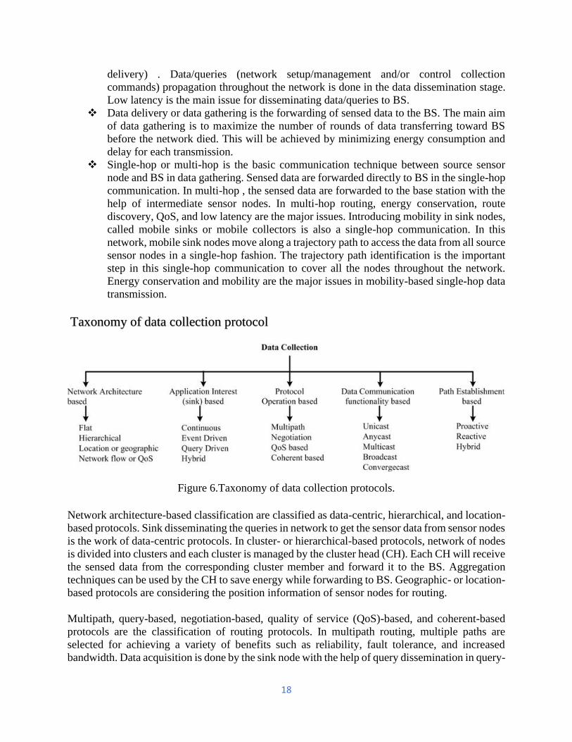
18
delivery) . Data/queries (network setup/management and/or control collection
commands) propagation throughout the network is done in the data dissemination stage.
Low latency is the main issue for disseminating data/queries to BS.
❖ Data delivery or data gathering is the forwarding of sensed data to the BS. The main aim
of data gathering is to maximize the number of rounds of data transferring toward BS
before the network died. This will be achieved by minimizing energy consumption and
delay for each transmission.
❖ Single-hop or multi-hop is the basic communication technique between source sensor
node and BS in data gathering. Sensed data are forwarded directly to BS in the single-hop
communication. In multi-hop , the sensed data are forwarded to the base station with the
help of intermediate sensor nodes. In multi-hop routing, energy conservation, route
discovery, QoS, and low latency are the major issues. Introducing mobility in sink nodes,
called mobile sinks or mobile collectors is also a single-hop communication. In this
network, mobile sink nodes move along a trajectory path to access the data from all source
sensor nodes in a single-hop fashion. The trajectory path identification is the important
step in this single-hop communication to cover all the nodes throughout the network.
Energy conservation and mobility are the major issues in mobility-based single-hop data
transmission.
Taxonomy of data collection protocol
Figure 6.Taxonomy of data collection protocols.
Network architecture-based classification are classified as data-centric, hierarchical, and location-
based protocols. Sink disseminating the queries in network to get the sensor data from sensor nodes
is the work of data-centric protocols. In cluster- or hierarchical-based protocols, network of nodes
is divided into clusters and each cluster is managed by the cluster head (CH). Each CH will receive
the sensed data from the corresponding cluster member and forward it to the BS. Aggregation
techniques can be used by the CH to save energy while forwarding to BS. Geographic- or location-
based protocols are considering the position information of sensor nodes for routing.
Multipath, query-based, negotiation-based, quality of service (QoS)-based, and coherent-based
protocols are the classification of routing protocols. In multipath routing, multiple paths are
selected for achieving a variety of benefits such as reliability, fault tolerance, and increased
bandwidth. Data acquisition is done by the sink node with the help of query dissemination in query-
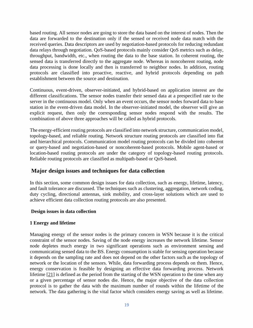
19
based routing. All sensor nodes are going to store the data based on the interest of nodes. Then the
data are forwarded to the destination only if the sensed or received node data match with the
received queries. Data descriptors are used by negotiation-based protocols for reducing redundant
data relays through negotiation. QoS-based protocols mainly consider QoS metrics such as delay,
throughput, bandwidth, etc., when routing the data to the base station. In coherent routing, the
sensed data is transferred directly to the aggregate node. Whereas in noncoherent routing, node
data processing is done locally and then is transferred to neighbor nodes. In addition, routing
protocols are classified into proactive, reactive, and hybrid protocols depending on path
establishment between the source and destination.
Continuous, event-driven, observer-initiated, and hybrid-based on application interest are the
different classifications. The sensor nodes transfer their sensed data at a prespecified rate to the
server in the continuous model. Only when an event occurs, the sensor nodes forward data to base
station in the event-driven data model. In the observer-initiated model, the observer will give an
explicit request, then only the corresponding sensor nodes respond with the results. The
combination of above three approaches will be called as hybrid protocols.
The energy-efficient routing protocols are classified into network structure, communication model,
topology-based, and reliable routing. Network structure routing protocols are classified into flat
and hierarchical protocols. Communication model routing protocols can be divided into coherent
or query-based and negotiation-based or noncoherent-based protocols. Mobile agent-based or
location-based routing protocols are under the category of topology-based routing protocols.
Reliable routing protocols are classified as multipath-based or QoS-based.
Major design issues and techniques for data collection
In this section, some common design issues for data collection, such as energy, lifetime, latency,
and fault tolerance are discussed. The techniques such as clustering, aggregation, network coding,
duty cycling, directional antennas, sink mobility, and cross-layer solutions which are used to
achieve efficient data collection routing protocols are also presented.
Design issues in data collection
1 Energy and lifetime
Managing energy of the sensor nodes is the primary concern in WSN because it is the critical
constraint of the sensor nodes. Saving of the node energy increases the network lifetime. Sensor
node depletes much energy in two significant operations such as environment sensing and
communicating sensed data to the BS. Energy consumption is stable for sensing operation because
it depends on the sampling rate and does not depend on the other factors such as the topology of
network or the location of the sensors. While, data forwarding process depends on them. Hence,
energy conservation is feasible by designing an effective data forwarding process. Network
lifetime [21] is defined as the period from the starting of the WSN operation to the time when any
or a given percentage of sensor nodes die. Hence, the major objective of the data collection
protocol is to gather the data with the maximum number of rounds within the lifetime of the
network. The data gathering is the vital factor which considers energy saving as well as lifetime.
20
In literature [4, 22], the authors have presented energy-efficient techniques for data collection.
Rault et al. [4] have reviewed the energy-saving techniques and its classification such as radio
optimization, data reduction, sleep/wake-up schemes, energy-efficient routing, and battery
repletion. Anastasi et al. [22] in 2009 discussed directions for energy conservation in WSNs and
presented the taxonomy of energy conservation techniques such as duty cycling, data driven, and
mobility-based routing
2. Latency
Latency is the period from the time unit that the data generation at the sensor node started to the
time unit that data reception was completed at the base station. It is one of the main concerns for
time significant applications such as military and medical health-care monitoring. Attaining low
latency is a vital concern because of the following reasons:
1. Due to limited constraints of sensor nodes which are more prone to failure.
2. Collisions and network traffic will be increased due to the broadcast nature of radio
channel.
3. Same kind of data will be sensed by densely deployed sensors and transfer to BS will
increase the network traffic and exhaust the communication bandwidth.
To deal with the above issues, there is a need for low-latency protocols.; such mechanisms are
sampling time, propagation time, processing time, scheduling, use of directional antennas, MAC
protocols, sleep/wake-up cycles, predictions, use of dual-frequency radios, etc. A review on
energy-efficient and low-latency routing protocols for WSNs without dominating the other design
factors
3.Fault tolerance
Fault tolerance enhances the availability, reliability, and dependability of the system by ensuring
the usage availability of the system without any disruption in the presence of faults. In WSN, fault
tolerance is also a demanding issue due to the sensor nodes more vulnerable to failure because of
energy depletions, desynchronization, communication link errors, etc., which are provoked owing
to hardware and software failures, environmental conditions, etc. Hence, fault management in
WSN must be administered with additional care. Initial review works on fault-tolerant routing
schemes are Three phases called fault diagnosis, fault detection, and fault recovery for supervising
faults have been proposed. In fault detection phase, an unexpected failure should be identified by
the system.. In fault diagnosis phase, comprehensive description or model has been determined to
distinguish various faults in WSNs or fault recovery action. In the fault recovery phase, the sensor
network is redesigned from failures or fault nodes to enhance the network performance.
COLLABRATIVE INFORMATION PROCESSING AND GROUP
CONNECTIVITY: • WSN evolved as a consequence of the advancements in several areas of research. These
are mainly: sensing, wireless communication and computing (including hardware,
software, and algorithms). Examples of early WSN include the radar networks used in air
21
traffic control. The national power grid, with its many sensors, can be viewed as one large
sensor network. These systems were developed with specialized computers and
communication capabilities, and before the term “wireless sensor networks” came into
vogue.
• The rapid progress of wireless communication and embedded micro sensing MEMS
technologies has made the development of WSN possible through the tiny, battery powered
nodes that have computational capabilities.
• The wireless nodes can communicate with each other and interact with their environment
in order to gather, process and convey the information. WSN are commonly referred to as
ad-hoc or decentralized wireless networks, due to their capability of forwarding data to
other nodes, and so the determination of which nodes forward data is made dynamically,
based on the network connectivity. The nodes in an ad-hoc wireless sensor network
collaborate to collect and process data to generate useful information.
• Collaborative signal and information processing over a network is a relatively new area of
research and is related to distributed information fusion. Important technical issues include
the degree of information sharing between nodes and how nodes fuse the information from
other nodes. Processing data from more sensors generally results in better performance but
also requires more communication resources (and, thus, energy).
• Less information is lost when communicating information at a lower level (e.g., raw
signals), but requires more bandwidth. Therefore, one needs to consider the multiple
tradeoffs between performance and resource utilization in collaborative signal and
information processing using wireless sensors. Other processing issues include how to
meet mission latency and reliability requirements, and how to maximize sensor network
operational life. A dense network of cheap sensors may allow spatial sampling without the
need for expensive algorithms. These algorithms must be asynchronous, as the processor
speeds and communication capabilities may vary or even disappear and reappear.
• Research and experience have shown that optimal collaboration among sensor nodes can
significantly improve the efficiency of sensing and processing in sensor networks. There
are instances when collections of nodes need to cooperate with each other in detection of
signals or events . In such instances, when a cooperative function is required to extract
information about a specific target, a local network is built to facilitate the necessary
signaling and data transfer tasks.
• Typically, cooperative functions involve a small set of nodes near the target location and
operate for relatively short time spans. They are required to adapt quickly and efficiently
to the appearance of the target and the nature of the signal processing techniques required.
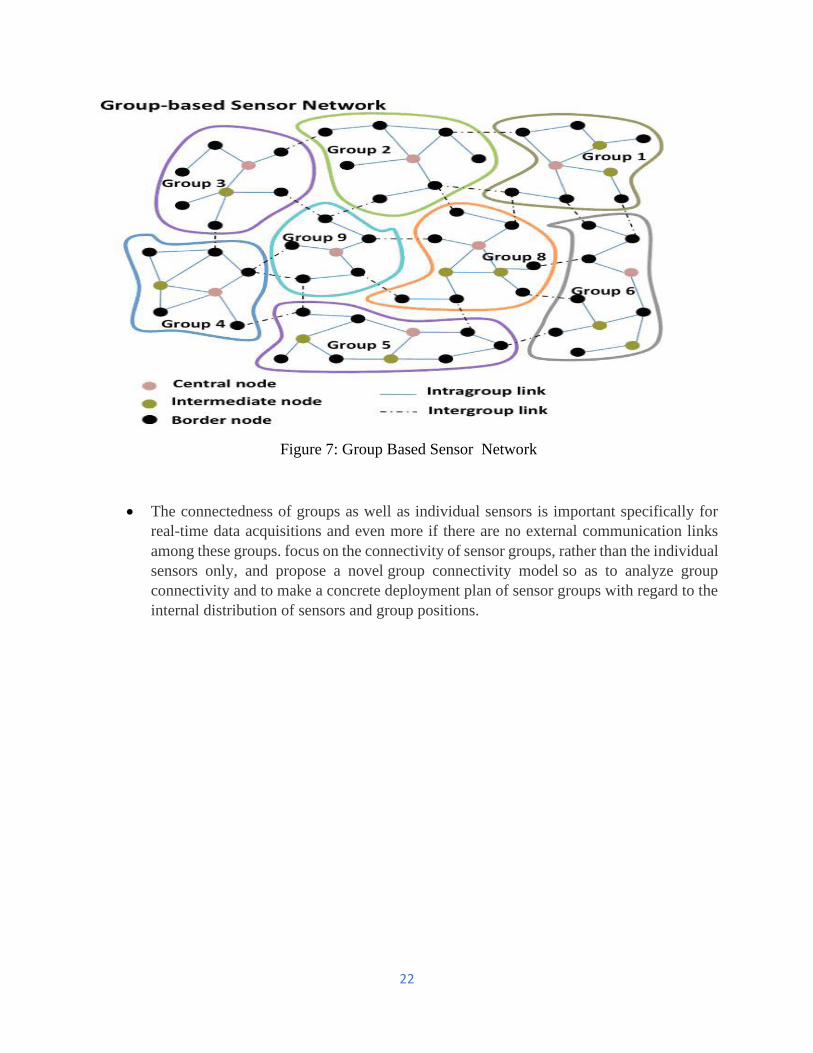
22
Figure 7: Group Based Sensor Network
• The connectedness of groups as well as individual sensors is important specifically for
real-time data acquisitions and even more if there are no external communication links
among these groups. focus on the connectivity of sensor groups, rather than the individual
sensors only, and propose a novel group connectivity model so as to analyze group
connectivity and to make a concrete deployment plan of sensor groups with regard to the
internal distribution of sensors and group positions.

1
SCHOOL OF COMPUTING
DEPARTMENT OF COMPUTER SCIENCE AND ENGINEERING
SCSA5202-WIRELESS SENSOR NETWORKS
Unit- I- WIRELESS SENSOR NETWORKS-SCSA5202

2
Unit V
SENSOR NETWORK TOOLS
Sensor Network Platforms and Tools: Sensor node hardware- Programming challenges-Node
level software platform-Node level simulators-Programming beyond individual nodes-Security-
Privacy issues-Attacks and counter measures.
Sensor Node Hardware and programing
Sensor Node Hardware:
Sensor node hardware can be grouped into three categories. Augmented general-purpose computers, Dedicated embedded sensor nodes,System-on-chip (SoC).Berkley motes due to their small form factor, open source software development, and commercial availability, have gained wide popularity in the sensor network research community. In order to keep the program footprint small to accommodate their small memory size, programmers of these platforms are given full access to hardware but barely any operating system support. Typically support at least one programming language, such as C.zEx: mica, TinyOS. Node-level software platforms
Node-centric design methodologies: Programmers think in terms of how a node should behave in the environment.zA node-level platform can be a node-centric OS, which provides hardware and networking abstractions of a sensor node to programmers.
TINY OS
Static memory allocation: analyzable, reduce memory management overheadzOnly parts of OS are compiled
with the application. A program executed in TinyOShas two contexts, tasks and events.zTasks are posted by
components to a task scheduler. Without preempting or being preempted by other taskszTriggered events can
be preempted by other events and preempt tasks
nesC
An event call is a method call from a lower layer component to a higher layer component. (signal)zA command
is the opposite. (call)zA component may use or provide the same interface multiple times. Give each interface inesCzAn application must contain the Main module which links the code to the scheduler at run time.zThe Main has a single StdControlinterface, which is the ultimate source of initialization of all componenstance a separate name using as notation.
Node-Level Simulators
• Wireless network are vulnerable to security attacks due to the broadcast nature of the transmission
medium.
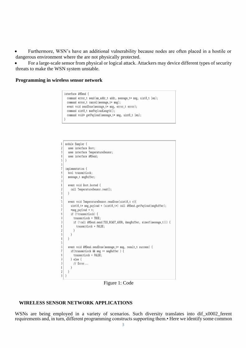
3
• Furthermore, WSN’s have an additional vulnerability because nodes are often placed in a hostile or
dangerous environment where the are not physically protected.
• For a large-scale sensor from physical or logical attack. Attackers may device different types of security
threats to make the WSN system unstable.
Programming in wireless sensor network
Figure 1: Code
WIRELESS SENSOR NETWORK APPLICATIONS WSNs are being employed in a variety of scenarios. Such diversity translates into dif_x0002_ferent requirements and, in turn, different programming constructs supporting them.• Here we identify some common
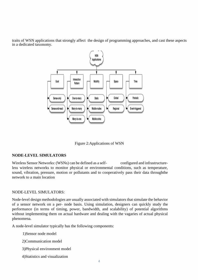
4
traits of WSN applications that strongly affect the design of programming approaches, and cast these aspects in a dedicated taxonomy.
Figure 2:Applications of WSN
NODE-LEVEL SIMULATORS
Wireless Sensor Networks: (WSNs) can be defined as a self- configured and infrastructure-
less wireless networks to monitor physical or environmental conditions, such as temperature,
sound, vibration, pressure, motion or pollutants and to cooperatively pass their data throughthe
network to a main location
NODE-LEVEL SIMULATORS:
Node-level design methodologies are usually associated with simulators that simulate the behavior
of a sensor network on a per- node basis. Using simulation, designers can quickly study the
performance (in terms of timing, power, bandwidth, and scalability) of potential algorithms
without implementing them on actual hardware and dealing with the vagaries of actual physical
phenomena.
A node-level simulator typically has the following components:
1)Sensor node model
2)Communication model
3)Physical environment model
4)Statistics and visualization
5
1)Sensor node model: A node in a simulator acts as a software execution platform, a
sensor host, as well as a communication terminal. In order for designers to focus on the application-
level code, a node model typically provides or simulates a communication protocol stack, sensor
behaviors (e.g., sensing noise), and operating system services. If the nodes are mobile, then the
positions and motion properties of the nodes need to be modeled. If energy characteristics are part
of the design considerations, then the power consumption of the nodes needs to be modeled.
2)Communication model: Depending on the details of modeling, communication may be captured
at different layers. The most elaborate simulators model the communication media at the physical
layer, simulating the RF propagation delay and collision of simultaneous transmissions. Alternately,
the communication may be simulated at the MAC layer or network layer, using, for example,
stochastic processes to represent low-level behaviors.
3)Physical environment model: A key element of the environment within which a sensor network
operates is the physical phenomenon of interest. The environment can also be simulated at various
levels of detail. For example, a moving object in the physical world may be abstracted into a point
signal source. The motion of the point signal source may be modeled by differential equations or
interpolated from a trajectory profile. If the sensor network is passive—that is, it does not impact
the behavior of the environment—then the environment can be simulated separately or can even
be stored in data files for sensor nodes to read in. If, in addition to sensing, the network also
performs actions that influence the behavior of the environment, then a more tightly integrated
simulation mechanism is required.
4) Statistics and visualization: The simulation results need to be collected for analysis. Since the
goal of a simulation is typically to derive global properties from the execution of individual
nodes, visualizing global behaviors is extremely important. An ideal visualization tool should
allow users to easily observe on demand the spatial distribution and mobility of the nodes, the
connectivity among nodes, link qualities, end-to-end communication routes and delays,
phenomena and their spatio-temporal dynamics, sensor readings on each node, sensor node
states, and node lifetime parameters (e.g., battery power).
->For engineers to perform study ,which in terms of Power and
Bandwidth
->A sensor network simulator simulates the behavior of a subset of the sensor nodes with respect
to time. Depending on how the time is advanced in the simulation, there are two types of execution
models:
cycle-driven simulation and discrete-event simulation. A cycle-driven (CD) simulation discretizes
the continuous notion of real time into (typically regularly spaced) ticks and simulates the system
behavior at these ticks. At each tick, the physical phenomena are first simulated, and then all nodes
are checked to see if they have anything to sense, process, or communicate. Sensing and
computation are assumed to be finished before the next tick.
That is, there should be no two components, such that one of them computes yk = f(xk) and the other computes xk = g(yk), for the same tick index k. In fact, one of the most subtle issues in designing a CD simulator is how to detect and deal with cyclic dependencies among nodes or algorithm components. Most
6
CD simulators do not allow interdependencies within a single tick. Synchronous languages [91], which are typically used in control system designs rather than sensor network designs, do allow cyclic dependencies. They use a fixed-point semantics to define the behavior of a system at each tick.
Unlike cycle-driven simulators, a discrete-event (DE) simulator assumes that the time is continuous and an event may occur at any time. An event is a 2-tuple with a value and a time stamp indicating when the event is supposed to be handled. Components in a DE simulation react to input events and produce output events. In node-level simulators, a component can be a sensor node and the events can be communication packets; or a component can be a software module within a node and the events can be message passings among these modules.
Typically, components are causal, in the sense that if an output event is computed from an input event, then the time stamp of the output event should not be earlier than that of the input event. Noncausal components require the simulators to be able to roll back in time, and, worse, they may not define a deterministic behavior of a system .A DE simulator typically requires a global event queue. All events passing between nodes or modules are put in the event queue and sorted according to their chronological order. At each iteration of the simulation, the simulator removes the first event (the one with the earliest time stamp) from the queue and triggers the component that reacts to that event.
In terms of timing behavior, a DE simulator is more accurate than a CD simulator, and, as a consequence, DE
simulators run slower. The overhead of ordering all events and computation, in addition to the values and time
stamps of events, usually dominates the computation time. At an early stage of a design when only the
asymptotic behaviors rather than timing properties are of concern, CD simulations usually require less
complex components and give faster simulations. Partly because of the approximate timing behaviors, which
make simulation results less comparable from application to application, there is no general CD simulator that
fits all sensor network simulation tasks. We have come across a number of home grown simulators written in
Matlab, Java, and C++. Many of them are developed for particular applications and exploit application-
specific assumptions to gain efficiency.
DE simulations are sometimes considered as good as actual implementations, because of their continuous
notion of time and discrete notion of events. There are several open-source or commercial simulators available.
One class of these simulators comprises extensions of classical network simulators, such as ns-2, J-Sim
(previously known as JavaSim), and GloMoSim/QualNet.8 The focus of these simulators is on network
modeling, protocols stacks, and simulation performance. Another class of simulators, sometimes
called software-in-the-loop simulators, incorporate the actual node software into the simulation. For this
reason, they are typically attached to particular hardware platforms and are less portable. Examples include
TOSSIM for Berkeley motes and Em* (pronounced em star)for Linux-based nodes such as Sensoria WINS
NG platforms.
Node-Level Simulator: ns-2 &TOSSIM:
ns-2
-Originally developed for wired networks
-Extensions for sensor nodes
-Node locations vs. logical addresses
7
-Energy models
-Physical phenomena
TOSSIM
-Simulator for TinyOS apps on Berkeley motes
-Compiles nesC source into simulator components
Programming beyond individual nodes:
->Applications more than simple distributed programs
-> Applications depend on state of physical environment
->Collaboration groups
-Set of entities that contribute to state updates
-Abstracts network topology and communication protocols
->Multi-target tracking problem
-Global state decoupled into separate pieces
-Each piece managed by different principal
- State updated by looking at inputs from other principals
-Collaboration groups define communication and roles
of each principal
Programming beyond individual nodes:
->The individual nodes in a wireless sensor network (WSN) are inherently resource constrained: they have limited processing speed, storage capacity, and communication bandwidth.
->After the sensor nodes are deployed, they are responsible for self- organizing an
appropriate network infrastructure often with multi-hop communication with them.
->Then the onboard sensors start collecting information of interest.
->Wireless sensor devices also respond to queries sent from a “control site”to perform specific instructions or
provide sensing samples.
-Applications that isn’t just simply generic distributed programs over an ad hoc network.
-We have to centralize data into nodes.
Def:
X:state of a system

8
U:inputs
Y:outputs
K:update index
F:state update function
G:output observation function
Security and Privacy Issues in Wireless Sensor Networks.
The sensor networks face a lot of challenges owing to the use of wireless medium for communication
which is prone to various types of attacks. There are various issues like energy exhaustion, memory and
storage shortage, security attacks. It is very important to safeguard the network for reliable
communication.
Why NEED SECURITY?
Wireless sensor networks have many applications in military, homeland security and other areas. In that
many sensor networks have mission-critical tasks. Security is critical for such networks deployed
in hostile environments.
Most sensor networks actively monitor their surroundings, and it is often easy to deduce information other
than the data monitored. Moreover, the wireless communication employed by sensor networks facilitates
eavesdropping and packet injection by an adversary. The combination of these factors demands security
for sensor networks at design time to ensure operation safety, secrecy of sensitive data, and privacy for
people in sensor environments. Providing security in sensor networks is even more difficult than
MANETs due to the resource limitations of sensor nodes.
WHY SECURITY IS COMPLICATED IN WSN?
• Overall cost of WSN should be as low as possible.
• Senor nodes are susceptible to physical capture.
• Sensor nodes use wireless communication, eavesdrop.
• Attacker can easily inject malicious message into network.
Anti-jamming and physical temper proofing techniques are impossible due to greater design
complexity and energy consumption.Sensor node constraints make WSN’S more susceptible to denial-
of service attack.Frequent topology changes of WSN facilities different link attacks ranging from
passive eavesdropping to active interfering.There is a conflict between resource consumption and
maximization of security level.Due to node constraints asymmetric cryptography is often too
expensive.Managing key distribution is not unique to WSN’s, but constraints such as small memory
capacity make centralized keying techniques impossible.
SECURITY REQUIREMENTS
• Confidentiality.
• Integrity.

9
• Availability.
• Freshness.
❖ Additional requirements:
• Authentication.
• Access-control.
• Privacy.
• Authorization.
• Non-repudiation.
• Survivability.
GUIDING PRINCIPLES FOR SECURING WSN?
• Security of a network is determined by the security over all layers.
• In a massively distributed network, security measure should be amenable to dynamic
reconfiguration and decentralized management.
• In a given network, at any given time, the cost incurred due to the security measures should not
exceed the cost assessed due to the security risks at that time.
• If physical security of nodes n a network is not guaranteed, the be carefully considered when
designing a security scheme: Power efficiency, Node Density and reliability, Adaptive Security,
Self-configurability, Simplicity and Local ID.
EVALUATION METRICS TO SECURITY SCHEME
• Security.
• Resiliency.
• Energy efficiency.
• Flexibility.
• Scalability.
• Fault-tolerance.
• Self-healing.
• Assurance.
TAXONOMY OF ATTACKS • Wireless network are vulnerable to security attacks due to the broadcast nature of the
transmission medium.
• Furthermore, WSN’s have an additional vulnerability because nodes are often placed in a
hostile or dangerous environment where the are not physically protected.
• For a large-scale sensor from physical or logical attack. Attackers may device different types
of security threats to make the WSN system unstable.

10
BASED ON CAPABILITY OF ATTACKER
• Outsider versus insider (Node Compromise) attack.
• Passive versus active attacks.
• Mote-class versus laptop-class attacks.
Attacks on Information in Transit
• Interruption
• Interception
• Modification
• Fabrication
• Replaying existing messages.
ISSUES WITH HIGH-LEVEL SECURITY MECHANISMS
CRYPTOGRAPH
To achieve security in WSNs, it is important to be able to perform various cryptographic operations, including encryption, authentication, and so on. However, decision for Selecting the appropriate cryptography method depends on the computation and communication capability of the sensor nodes. Asymmetric cryptography is often too expensive for many applications. Thus, a promising approach is to use more efficient symmetric cryptographic alternatives. However, symmetric cryptography is not as versatile as public key cryptographic techniques, which complicates the design of secure applications. Applying any encryption scheme requires transmission of extra bits, hence extra processing, memory and battery power, which are very important resources for the sensors’ longevity. Applying the security mechanisms such as encryption could also increase delay, jitter and packet loss in WSNs.
The process by which public key and symmetric key cryptography schemes should be selected is
based on the following criteria:
▪ Energy
11
▪ Program memory
▪ Temporary memory
▪ Execution time
▪ Program parameters memory
PURPOSE OF SENSOR NETWORK TOOLS
A WSN aims to gather environmental data and the node devices placement may be known or unknown a
priori. Network nodes can have actual or logical communication with all devices; such a communication
defines a topology according to the application
WHY SECURITY IS NEEDED
Attacks Sensor networks are particularly vulnerable to several key types of attacks. Attacks can be
performed in a variety of ways. Wireless networks are vulnerable to security attacks due to the broadcast
nature of the transmission medium. Furthermore, WSNs have an additional vulnerability because nodes
are often placed in a hostile or dangerous environment where they are not physically protected. For a
large-scale sensor network, it is impractical to monitor and protect each individual sensor from physical
or logical attack. Attackers may device different types of security threats to make the WSN system
unstable.
MAJOR CLASSIFICATION OF ATTACKS IN WSN TOOLS
1) Capability of Attackers
2) Attack on Information in Transit
3) Protocol Stack
Outside Attacks Are Defined As Attacks From Nodes, Which Do Not Belong Wsn. Insider Attacks Occur
When Legitimate Nodes Of A Wsn Behave In Unintended Or Unauthorised Ways. Passive Attacksit Refers
To Monitoring Packets Exchanged Within Wsn. Active Wsn It Involves Some Modifications Of The Data
Stream Or The Creation Of A Fake Streams. In Mote-Class Attacks An Advesary Attacks A Wsn By Using
A Few Nodes With Similar Capabilities To The Network Nodes. Laptop-Class Attacks An Advesary Can
Use More Powerful Devices (Eg- Laptop) To Attack A Wsn
ATTACKS ON INFORMATION IN TRANSIT
Software Compromise: This Involves Breaking The Software Running On The Sensor Nodes. Chances Are
The Operating System Or The Applications Running In A Sensor Node Are Vulnerable To Popular
12
Exploits Such As Buffer Overflows. It Has Two Orthogonal Perspectives Layer Specific Compromises
And Protocol Specific Compromises.This Includes All The Attacks On Information In Transit , It Also
Includes Deviating From Protocol
Attacks in the Physical Layer
Many attacks target this layer as all upper layer functionalities rely on it. Adversaries can do “non-
technical” things such as destroying sensors, or conduct“technical” actions such as wiretapping. In general,
the following three types of attacks are categorized as physical layer attacks:
• Device Tampering
• Eavesdropping
• Jamming
Device Tampering: As imaginable, the simplest way to attack is to damage or modify sensors physically and
thus stop or alter their services. The negative impact will be greater if base stations or aggregation points
instead of normal sensors are attacked, since the former carry more responsibility of communications and/or
data processing. However, the effectiveness of these attacks against physical sensors is very limited due to
the high redundancy inherent in most WSNs. Unless large amount of sensors are compromised, the
operations of WSNs will not be affected much. Another way to attack is to capture sensors and extract
sensitive data from them. As more complicated attacks (e.g. spoofing and denial of services) are made
possible by this step (based on the sensitive data), such attacks are probably more threatening.
Eavesdropping: Without senders and receivers’ awareness, eavesdropping attackers monitor the traffic in
transmission on communication channels and collect data that can later be analyzed to extract sensitive
information. WSNs are especially vulnerable to such attacks since wireless transmission is the dominant
method of communication used by sensors. During transmission, wireless signals are broadcast in the air and
thus accessible to the public. With modest equipment, attackers within the sender’s transmission range can
easily plug themselves into the wireless channel and obtain raw data. By and large, the capability of
eavesdropping depends on the power of antennas. The more powerful the antennas, the weaker signals
attackers can receive, and thus the more data can be collected. Since eavesdropping is a passive behavior,
such attacks are rarely detectable.
Jamming: Unlike device tampering attacks that are physical, jamming attacks disrupt the availability of
transmission media. The approach is to introduce intense interference to occupy the channels and bereave
normal sensors of the chances to communicate. With a device jamming its surrounding sensors, adversaries
can disrupt an entire sensor network by deploying enough number of such devices. The problem of such
attacks is that jamming devices have the risk of being identified, since sensors close to a jamming device
may detect higher background noise than usual.
Countermeasures in the Physical Layer
Some attacks in the physical layer are quite hard to cope with. For example, after sensors are deployed in the
field, it is difficult or infeasible to prevent every single sensor from device tampering. Therefore, although
there are some mechanisms that attempt to reduce the occurrences of attacks, more of them focus on
protecting information from divulgence.

13
Access Restriction: Obviously, restricting adversaries from physically accessing or getting close to sensors
is effective on all the attacks aforementioned. It is good to have such restrictions if we can, but unfortunately,
they are either difficult or infeasible in most cases. Therefore, we usually have to fall back on another type
of restrictions: communication media access restriction. A few techniques exist nowadays that prevent
attackers from accessing the wireless medium in use, including sleeping/hibernating and spread spectrum
communication [7]. The former is fairly simple as it switches off sensors and keeps them silent until the
attackers go away. However, its effectiveness is at the expense of sacrificing the operations of WSNs. The
latter is more intelligent, with frequencies varying deliberately. This technique uses either analog schemes
where the frequency variation is continuous, or digital schemes (e.g. frequency hopping) where the frequency
variation is abrupt. By this way, attackers cannot easily locate the communication channel, and are thus
restrained from attacking. With current technology, powerful devices are required to perform such
functionalities. Therefore, spread spectrum communications are not yet feasible for WSNs that are usually
constrained in resources. Nonetheless, given the rapid advancement of technologies, this technique is very
promising in the future. Directional antenna [is another technique for access restriction. By confining the
directions of the signal propagation, it reduces the chances of adversaries accessing the communication
channel. Again, similar to spread spectrum 5 communication, its production cost is high at present and
unsuitable for large-scale sensor networks, but may be more useful in the long run.
Encryption: In general, cryptography is the all-purpose solution to achieve security goals in WSNs. To
protect data confidentiality, cryptography is indispensable. Cryptography can be applied to the data stored
on sensors. Once data are encrypted, even if the sensors are captured, it is difficult for the adversaries to
obtain useful information. Of course, the strength of the encryption depends on various factors. A more
costly encryption can yield higher strength, but it also drains the limited precious energy faster and needs
more memory. More often, cryptography is applied to the data in transmission. There are basically two
categories of cryptographic mechanisms: asymmetric and symmetric. In asymmetric mechanisms (e.g. RSA
[13, 14, 15]), the keys used for encryption and decryption are different, allowing for easier key distribution.
It usually requires a third trusted party called Certificate Authority (CA) to distribute and check certificates
so that the identity of the users using a certain key can be verified. However, due to the lack of a priori trust
relationship and infrastructure support, it is infeasible to have CAs in WSNs. Furthermore, asymmetric
cryptography usually consumes more resources such as computation and memory
Attacks in the MAC Layer
Due to the openness of wireless channels, the coordinations between sensors based on MAC protocols are
subject to malicious manipulation. Adversaries can disobey the coordination rules and produce malicious
traffic to interrupt network operations in the MAC layer. They can also forge MAC layer identifications and
masquerade as other entities for various purposes.
Traffic Manipulation: The wireless communication in WSNs (and other wireless networks) can be easily
manipulated in the MAC layer. Attackers can transmit packets right at the moment when legitimate users do
so to cause excessive packet collisions. The timing can be readily decided by monitoring the channel and
doing some calculations based on the MAC protocol in effect. The artificially increased contention will
decrease signal quality and network availability, and will thus dramatically reduce the network throughput
Besides, in widely used MAC schemes where packet transmissions are carefully coordinated, attackers can
compete for channel usage aggressively disobeying the coordination rules.This misbehavior can break the
14
operations of the protocols and result in unfair bandwidth usage. In either way, the network performance is
degraded. Eventually, the collisions and unfairness lead traffic distortion.
Identity Spoofing: MAC identity spoofing is another common attack in the MAC layer.Due to the broadcast
nature of wireless communications, the MAC identity (such as a MAC address or a certificate) of a sensor
is open to all the neighbors, including attackers. Without proper protection on it, an attacker can fake an
identity and pretend to be a different one. A typical MAC identity spoofing attack is the Sybil attack.
CounterMeasures:
Misbehavior Detection Because attacks deviate from normal behaviors, it is possible to identify attackers by
observing what has happened. Various data can be collected for this purpose, and various actions can be
taken after detection. In a countering scheme for the IEEE 802.11 protocol, a receiver assigns and adjusts
the backoff values to be used by the corresponding sender. Whenever detecting the sender’s misbehavior in
manipulating backoff value, the receiver may add some penalty to the next backoff value assigned to the
sender. The idea was applied to ad hoc networks similarly can also be applied to WSNs. Another solution
uses “watchdogs” on every node to monitor whether or not the neighbors of a node forward the packets sent
out by this particular node. A neighbor not forwarding packets will be identified by the watchdog as a
misbehaving node.