Forthcoming: Journal of Development Economics

SCHOOL FEEDING AND LEARNING ACHIEVEMENT:EVIDENCE FROM INDIA’S MIDDAY MEAL PROGRAM

TANIKA CHAKRABORTY AND RAJSHRI JAYARAMAN

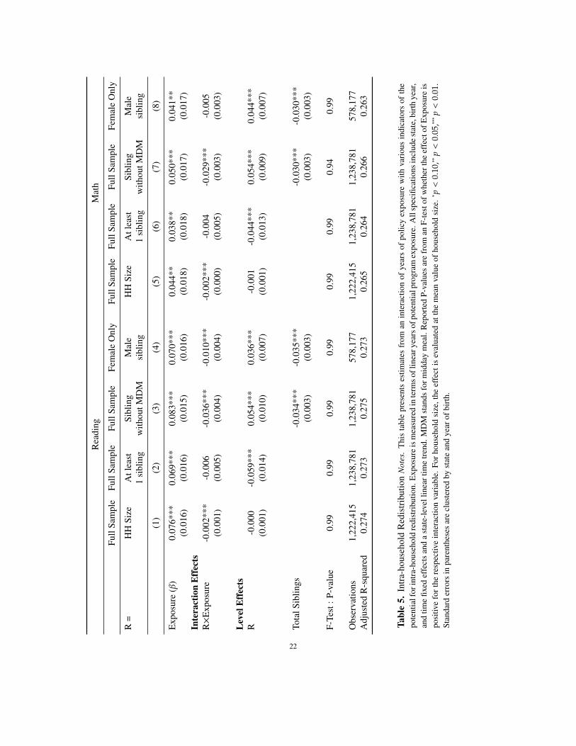
ABSTRACT. We study the effect of the world’s largest school feeding program on children’s learningoutcomes. Staggered implementation across different states of a 2001 Indian Supreme Court Directivemandating the introduction of free school lunches in public primary schools generates plausibly exoge-nous variation in program exposure across different birth cohorts. We exploit this to estimate the effectof program exposure on math and reading test scores of primary school-aged children. We find thatprolonged exposure to midday meals has a robust positive effect on learning achievement. We furtherinvestigate various channels that may account for this improvement including complementary school-ing inputs, heterogeneous responses by socio-economic status, and intra-household redistribution.

JEL Classification: I21, I25, O12

Keywords: school feeding, learning, midday meal, primary school education

Date: September 2018.

1. INTRODUCTION

School feeding programs are ubiquitous. The World Food Program estimated that in 2013, 368million children, or one in five, received a school meal at a total cost of US$ 75 billion (WFP, 2013).There are two main rationales for this sizable investment. The first is to abate hunger and improvehealth and nutrition. The second is to improve schooling outcomes.

This paper analyzes the latter by evaluating the impact of India’s free school lunch program—whichwe will refer to by its local moniker, “midday meals”—on learning achievements of primary schoolchildren. Importantly, we examine the effect of long-term program exposure of up to five years, onlearning outcomes. Proponents argue that free in-school feeding programs have a positive impacton learning through two main channels. First, they encourage school participation in the form ofschool enrollment or attendance. The latter in particular affords children the opportunity to learn inthe first place. Second, they improve children’s nutritional intake; alleviation of short-term hungerfacilitates concentration, and improved health and nutritional status leads to better cognition andlower absenteeism due to illness.

However, these positive effects are not self-evident for three reasons. First, complementary schoolinginputs, such as teachers or school infrastructure, are presumably needed in order to translate poten-tial increases in school participation and improvements in nutrition into better learning outcomes.Second, if children are already well-nourished (e.g. because they come from wealthy families), thenschool feeding may not provide any added benefit. Third, the program may not actually improve achild’s nutritional status if school meals induce families to substitute food away from a school-goingchild towards other family members. In addition to our main treatment effects, we explore each ofthese channels.

The Indian context we study is important for three reasons. First, the learning deficit in primaryschools is large. An ASER (2005) report, for example, revealed that 44% of children between theages of 7 and 12 who were actually enrolled in school could not read a basic paragraph and 50%could not do simple subtraction. Second, the scale of the intervention is massive: India’s middaymeal scheme is the largest school nutrition program in the world. In 2006, it provided lunch to 120million children in government primary schools on every school day (Kingdon, 2007). To put thisnumber in perspective, it accounts for one third of children globally who, according to the WFP(2013), enjoy school feeding programs. Finally, undernutrition is a severe problem in the country.India has some of the worst anthropometric indicators of nutrition in the world. According to the2005-6 National Family Health Survey (NFHS-3), 48% of children under the age of 5 were con-sidered chronically malnourished. Comparable data from 40 other developing countries covered bythe Demographic and Health Surveys (DHS) indicates that this proportion is higher in India than inany of those other countries. Undernourishment during childhood has been well-documented to havedeleterious lifetime consequences. In this context, school feeding programs have a potentially vitalrole to play in combating undernutrition.

In order to identify the causal effect of this program, we exploit its staggered implementation. Briefly,and in more detail later, a 2001 Indian Supreme Court directive ordered Indian states to institute freemidday meals in government primary schools. Prior to 2001 only two states, Tamil Nadu and Gujarat,had universal public primary school midday meal provision. Over the subsequent five years, however,state governments across India introduced midday meals. Staggered implementation of the program

1

in primary schools generates variation in the length of potential exposure to the program based ona child’s birth cohort and state of residence. Children only enjoyed the program to the extent thatthey were of primary-school going age—6 to 10 years old—and lived in a state which had institutedmidday meals in primary school. Hence, the earlier their state introduced the program and the youngenough they were at the time, the longer was the child’s potential exposure to midday meals in thisintent-to-treat (ITT) framework.

Although our quasi-experimental empirical design has some advantages that we elaborate on below,its obvious disadvantage is that identification is not as clean as it is in experimental studies. Ourmain identifying assumption is that there are parallel trends in learning achievement within cohortsbetween early and late program implementers. We present evidence that the timing of implementa-tion was plausibly exogenous to state-level characteristics; the descriptive analysis suggests that thestronger assumption of parallel trends in average outcomes between early and late implementers isplausible; and our results are robust to a number of specification checks pertaining to the timing ofimplementation. However, in keeping with all difference-in-differences-type empirical strategies, wemust concede that we cannot formally test this assumption.

Our data come from the Annual Status of Education Report (ASER) survey, whose goal is to as-sess the state of education among children in India. It has three unique features that are useful forthe purpose of this analysis. First, it has wide geographic coverage, surveying over 200,000 house-holds across India’s roughly 580 rural districts. Second, it has been administered annually since2005. Third, ASER administers learning assessments of basic literacy (reading skills) and numer-acy (number recognition and arithmetic skills) to all children aged 5 to 16. These features allow usto capture variation in exposure to treatment across states and time, while correcting for state- andcohort-specific effects as well as state-specific time trends, in order to assess the program’s effect onlearning. State fixed effects allow for average test scores to vary across different states, accountingfor the possibility that children in better or worse performing states may have longer program ex-posure because their states implemented the program earlier or later. Cohort fixed effects addressthe concern that older children are likely to have higher test scores than younger children, and alsopotentially have longer program exposure. Finally, the inclusion of state-specific time trends permitsfor trends in average test performance to vary from state to state.

We find that exposure to midday meals increases students’ learning achievement, albeit at a decreas-ing rate. Children with up to five years of exposure have reading test scores that are 18% higher, andmath test scores that are 9% higher than students with less than a year of exposure. In terms of po-tential channels, when we explore complementarities, we find that schooling inputs that are directlyrelated to teaching are associated with significantly higher learning when combined with a middaymeal, but more general schooling infrastructure is not. At the same time, we find no evidence ofheterogeneous treatment effects on the basis of gender or housing assets. Finally, we find limitedevidence of intra-household redistribution from eligible children to other family members.

The benefits of the midday meal program in terms of test score improvements are roughly comparableto some recent interventions aimed at improving the test performance of primary school children inIndia, in particular the introduction of extra teachers (Muralidharan and Sundararaman, 2013) andtutoring (Banerjee et al., 2007). On the one hand, this is impressive given that improved schoolperformance is, if anything, a side benefit of a program whose primary goal was to improve children’snutritional status. On the other hand, this improvement comes at a cost per child that is almost three

2

times higher than these teaching and tutoring inputs. As a consequence, midday meals underperformrelative to these programs in terms of test score improvements per dollar spent.

Related Literature. There is a substantial literature on the effect of school feeding programs onschool participation and nutritional outcomes; see Alderman and Bundy (2012) for an excellent re-view. Most of these studies have focused on young, typically primary-school-aged children, and havegenerally found that there are positive treatment effects on both participation (e.g. higher schoolenrollment or attendance) and nutritional status (e.g. lower anemia or higher BMI).1

The focus of this paper is to examine the effects of school feeding on learning achievement. It speaksto two main strands of this literature. The first strand has examined the effect of school feedingprograms on learning achievement in the context of small-scale, relatively short-term, randomizedfield experiments.2 Most of these experiments find no effect on cognitive achievement. A handfulthat reports improvements finds it only for narrowly defined subsets of students on a subset of skills.

The second strand of the literature has explored the effect of India’s midday meal program on chil-dren’s nutritional and schooling outcomes using quasi-experimental methods. To the best of ourknowledge, only two studies have examined its effect on learning outcomes, both using variation atthe local level.3 Singh (2008) finds improvements in Peabody Picture Vocabulary Tests in the YoungLives panel of about 500 children in Andhra Pradesh. However, he is cautious in the interpretationof this result since he lacks a control group in the analysis. Afridi et al. (2014) use the extension ofmidday meals to upper primary school (grades 6-8) in educationally “backward” localities to evaluateits effect on learning outcomes of 400 students in 16 Delhi schools using difference-in-differences.The authors find a significant improvement in classroom attention. However, in the 4-month timeframe of their study, they find no improvement in academic test scores.

We contribute to these two strands of literature in a couple of ways. First, whereas extant evidencehas focused on relatively short-term effects—anywhere from a few weeks to at most two years—weexplore the effect of up to five years of program exposure. Second, we use a large dataset. This notonly affords us statistical power but also allows us to study an intervention that has been implementedon a massive scale. The fact that the intervention is in no way “gold-plated”, combined with our useof a large data set that is representative of rural India also arguably adds to the generalizability of ourfindings.

Our results are in line with the extant literature, in that we find negligible or no positive effects ofmidday meals on learning outcomes in the short run. However, in contrast to most of this literature,

1See, for example, Jacoby et al. (1998), Powell et al. (1998), Van Stuijvenberg et al. (1999), Jacoby (2002), Neumannet al. (2003), and Bhattacharya et al. (2006), who generally find positive effects of school feeding programs on children’shealth and nutritional status. Jacoby et al. (1998), Powell et al. (1998), Ahmed (2004), Kremer and Vermeersch (2005),Belot and James (2011), Kazianga et al. (2012) find positive effects of school feeding programs on school participation.

2See Kazianga et al. (2012), Powell et al. (1998), Van Stuijvenberg et al. (1999), Grantham-McGregor et al. (1998),Adelman et al. (2008), Neumann et al. (2007), Kremer and Vermeersch (2005), and Whaley et al. (2003). In a rare non-randomized evaluation of an extant national program, McEwan (2013) uses a regression discontinuity design to studythe effect of Chile’s long-established school feeding program on (among other things) fourth-grade test scores. The dis-continuity comes from the fact that students received meals with different caloric content depending on a school-level“vulnerability” index cutoff. McEwan (2013) finds that there is no difference in test performance when the caloric contentof meals is increased.

3Others have examined the effect of midday meals in India on school participation and nutritional outcomes; see Afridi(2010), Singh et al. (2014), Afridi (2011) and Jayaraman and Simroth (2015).

3

we find an unambiguously positive effect of school feeding after the almost five-year exposure pe-riod, measured by both reading and math test scores. There are three possible explanations for thedifference between our findings and the previous literature. First, small sample sizes may accountfor imprecise estimates of positive effects in earlier studies. Our large dataset allows us to evade thisproblem. Second, the gains that we observe due to long-term exposure may not be fully capturedin many of the shorter-term interventions that have been evaluated to date. The empirical design ofthis paper is not equipped to provide a definitive answer for why this discrepancy between short- andlong-term exposure exists; that is left to future research. Conceptually, however, cognitive ability hasbeen shown to be associated with cumulative nutrition, as measured in height or height-for-age, andit is likely that the long-term exposure we investigate here captures just that.4 Moreover, as King andBehrman (2009) have argued in the context of natural policy settings such as ours, there may be lagsin implementation, or learning and adjustment to social programs. On the provider side, setting upand operating a school feeding program is logistically challenging in terms of both physical inputssuch as food delivery and cooking, and personnel management of teachers and cooks. On the benefi-ciaries side, learning and adoption by parents and students may also take time. Both of these lags maymean that a program which is otherwise effective in the long-run, may not appear so in the short-run.

The third explanation for why we find positive treatment effects while others often haven’t, is thecontext we study. Our data come from villages in rural India where nutritional deficiency is a chronicproblem. Using National Sample Survey (NSS) data, Deaton and Dreze (2009) calculate that in 2004-5—the first year of observation in our data—almost 80% of the rural population lived in householdswith a per capita calorie consumption below the rural poverty line of 2,400. It is conceivable that thesizable gains in learning achievement that we find reflect the fact that the target population of thisintervention in our sample is extremely nutritionally disadvantaged to begin with. This would be inline with the findings of Powell et al. (1998), Van Stuijvenberg et al. (1999) and Grantham-McGregoret al. (1998). It is also consistent with the fact that we find no heterogeneous treatment effects interms of gender or household assets, in that the bulk of children in our data are likely to suffer fromsubstantial economic disadvantage.

The rest of the paper is organized as follows. Section 2 furnishes the policy background. Section3 describes our data and empirical model. The main result—the effect of midday meals on testscores—is presented in Section 4. Section 5 delves into some channels that may drive the increase intest scores. Section 6 describes a series of robustness checks on our main result from Section 4, andSection 7 concludes with a cost-benefit analysis.

2. POLICY BACKGROUND

The Indian central government has a long-standing commitment to on-site school feeding programs.5

In 1995, the central government mandated free cooked meals in all public primary schools via the Na-tional Program of Nutritional Support to Primary Education. In India, the central government’s role

4See, for example, Case and Paxson (2008a,b), Schick and Steckel (2010), Karp et al. (1992) and in the Indian context,Spears (2012).

5The description of the natural experiment in this section draws, in part, from Jayaraman and Simroth (2015), whoexploit the same policy setting that we do. However, the question we address, the data, the empirical strategy, and theanalysis are completely different.

4

in school education lies in issuing policy guidelines and providing funding. Policy implementation isthe prerogative of state governments, and not a single state responded to this universal mandate.6

Half a decade later, India witnessed a sea change. In early 2001 there was a severe drought in7 districts, to which the press and many civil society organizations attributed a number of starvationdeaths.7 In April 2001, the People’s Union for Civil Liberties (PUCL) took the government of India tocourt, arguing in its writ petition that, “while on the one hand the stocks of food grains in the countryare more than the capacity of storage facilities, on the other there are reports from various statesalleging starvation deaths.”8 The PUCL documented that it was perfectly feasible for the governmentto widen a number of statutory food and nutrition programs, including the moribund midday mealscheme in schools. In response to this petition, on November 28, 2001, the Indian Supreme Courtissued an interim order stating that “Every child in every government and government-assisted schoolshould be given a prepared midday meal”.9

Implementation of this and other Supreme Court orders lies in the hands of the relevant executivebranch of government, which in this instance was state governments (Desai and Muralidhar, 2000).Midday meal implementation did not take place immediately or all at once, but over the next 5years states across India implemented the program until, by 2006, every Indian state had instituteda free school lunch in primary schools. Appendix Table 1 documents the month and year of policyimplementation in the 24 states and union territories used in our main analysis; the map in Figure A1of the Online Appendix depicts geographic variation in the timing of implementation. Tamil Nadu,Gujarat, Puducherry and Kerala are excluded from this sample since their program implementationpreceded the 2001 mandate, but we show in robustness checks that their inclusion does not alter ourresults. The table shows that there is considerable variation in the timing of implementation acrossdifferent states. As we explain later, this will be key to our identification strategy.

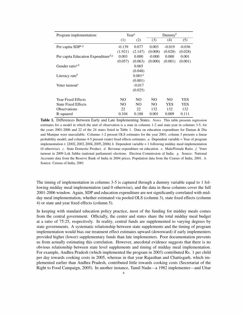
It is worth noting that there appears to be no significant correlation between the timing of imple-mentation and a number of observed state-level variables. This is evident in Table 1, which usesstate-level data from 2001 to 2006—the window over which the program was introduced and imple-mented. The first 2 columns present the results of an OLS regression for states in our main samplein 2001.10 This was the year of the Supreme Court directive, and the year before the earliest statesimplemented the program. The first 2 columns regress the year of midday meal implementation ona number of state-level covariates in this baseline year. These include economic indicators such asstate domestic product (SDP) and education expenditure, as well as social and civic indicators suchas the gender ratio, literacy rates, and voter turnout. None are statistically significant at the 5% level(only literacy is statistically significant at the 10% level, but the coefficient is close to zero.)

6Kerala responded with an opt-in program for public primary schools, leading to partial coverage. Tamil Nadu andGujarat had, in 1982 and 1984 respectively, already instituted universal primary school midday meal programs. Mostother states provided raw wheat or rice grains to enrolled children who attended school. Most accounts indicate that thissystem did not function well: grains were of poor quality, conditional attendance requirements were on paper alone (seefor example Probe Team (1999)), and the system was plagued with leakage (see for example Muralidharan (2006)).

7There were 7 drought-affected states in 2001: Gujarat, Rajasthan, Maharashtra, Orissa, Madhya Pradesh, Chhattisgarh,and Andhra Pradesh (Down to Earth, Vol. 10, Issue 20010615, June 2001). They include both early and late implementersof midday meals.

8Rajasthan PUCL Writ in Supreme Court on Famine Deaths, PUCL Bulletin, November 2001.9Supreme Court Order of November 28, 2001, Record of Proceedings Writ Petition (Civil) No. 196 of 2001.10Daman & Diu as well as Manipur are excluded from this sample since they lack education expenditure data.

5

Program implementation: Yeara Dummyb

(1) (2) (3) (4) (5)

Per capita SDPc,g -0.139 0.077 0.003 -0.019 -0.036(1.921) (2.147) (0.008) (0.028) (0.028)

Per capita Education Expenditured,g 0.003 0.000 -0.000 0.000 0.001(0.057) (0.063) (0.000) (0.001) (0.001)

Gender ratioe,h 0.065(0.048)

Literacy rateh 0.001*(0.001)

Voter turnoute -0.017(0.025)

Year Fixed Effects NO NO NO NO YESState Fixed Effects NO NO NO YES YESObservations 22 22 132 132 132R-squared 0.104 0.188 0.001 0.009 0.111

Table 1. Differences Between Early and Late Implementing States. Notes. This table presents regressionestimates for a model in which the unit of observation is a state in columns 1-2 and state-year in columns 3-5, forthe years 2001-2006 and 22 of the 24 states listed in Table 1. Data on education expenditure for Daman & Diuand Manipur were unavailable. Columns 1-2 present OLS estimates for the year 2001; column 3 presents a linearprobability model; and columns 4-5 present (state) fixed effects estimates. a. Dependent variable = Year of programimplementation ∈ {2002, 2003, 2004, 2005, 2006} b. Dependent variable = 1 following midday meal implementation(0 otherwise). c. State Domestic Product. d. Revenue expenditure on education. e. Male/Female Ratio. f. Voterturnout in 2009 Lok Sabha (national parliament) elections. Election Commission of India. g. Source: NationalAccounts data from the Reserve Bank of India in 2004 prices, Population data from the Census of India, 2001. h.Source: Census of India, 2001

The timing of implementation in columns 3-5 is captured through a dummy variable equal to 1 fol-lowing midday meal implementation (and 0 otherwise), and the data in these columns cover the full2001-2006 window. Again, SDP and education expenditure are not significantly correlated with mid-day meal implementation, whether estimated via pooled OLS (column 3), state fixed effects (column4) or state and year fixed effects (column 5).

In keeping with standard education policy practice, most of the funding for midday meals comesfrom the central government. Officially, the center and states share the total midday meal budgetat a ratio of 75:25, respectively. In reality, central funds are supplemented to varying degrees bystate governments. A systematic relationship between state supplements and the timing of programimplementation would bias our treatment effect estimates upward (downward) if early implementersprovided higher (lower) supplementary funds than late implementers. Poor documentation preventsus from actually estimating this correlation. However, anecdotal evidence suggests that there is noobvious relationship between state level supplements and timing of midday meal implementation.For example, Andhra Pradesh (which implemented the program in 2003) contributed Rs. 1 per childper day towards cooking costs in 2005, whereas in that year Rajasthan and Chattisgarh, which im-plemented earlier than Andhra Pradesh, contributed little towards cooking costs (Secretariat of theRight to Food Campaign, 2005). In another instance, Tamil Nadu—a 1982 implementer—and Uttar

6

Pradesh—a 2004 implementer—were both reported to have allocated the largest (state) budgets perchild per day towards midday meals in 2009-2010 (Centre for Policy Research, 2013).

In what follows, we describe central government funding provisions, which are more transparentlydocumented. Food grains are provided by the Food Corporation of India (FCI), an institution set upin 1964 to support the operation of the central government’s food policies. Midday meal guidelinesstipulate that each student be provided 100 grams of wheat or rice, 20 grams of pulses, 50 grams ofvegetables and 5 grams of fat per day, amounting to a targeted total of 300 kilo calories and 8-12grams of protein (MHRD, MHRD). As of 2009, this cost approximately Rs. 2.5 per student per day,including cooking costs.11 In addition to the direct cost of food, the cost of labor and management,which include salaries paid to cooks and helpers, adds another Rs. 0.40, for a total cost of foodequal to Rs. 2.90 per child per day. Of this, the central government provides Rs 2.17 and states areleft to bear the remaining Rs. 0.63. Further, the central government provides a transport subsidyto carry grains from the nearest FCI warehouse to the primary school, up to a maximum of Rs. 75per quintal, amounting to an average transport subsidy of Rs. 0.075 per child per school day. Anadditional budget of approximately 2% of total cost is assigned by the central government for themanagement, monitoring and evaluation of the program, amounting to an additional Rs. 0.045 perchild per day. The total value of the central government subsidy therefore amounted to Rs. 2.30. Thisis approximately 5 U.S. cents per child per school day, or 10 USD per child per year.12

While the overall responsibility for program implementation rests with state governments, day-to-dayoperations lie in the hands of local government bodies, typically village governments (panchayats),who sometimes delegate implementation to local Parent Teacher Associations (PTAs) or NGOs. Themeal itself is not extravagant. It is cooked at schools by cooks and their helpers, who are hired for thispurpose. At around noon, children are served cooked rice or wheat, depending on the local staple,mixed with lentils or jaggery, and sometimes supplemented with oil, vegetables, fruits, nuts, eggs ordessert at the local level. The menu varies from place to place, but anecdotal evidence suggests thatchildren generally enjoy the opportunity to sit with their peers and eat their midday meals (see, forexample, Dreze and Goyal (2003)).

3. DATA AND EMPIRICAL STRATEGY

3.1. Data. Our data come from the Annual Status of Education Report (ASER), a yearly surveydevoted to documenting the status of education among children in rural India. The data comprisea repeated cross-section. Each year, the survey is conducted around October and covers a randomsample of 20-30 households per village in 20 villages in each of India’s roughly 580 rural districts.

What makes ASER truly unique is that it tests all children in the household between the ages of 5and 16 for reading and math proficiency using rigorously developed testing tools. The fact that thesurvey is administered in households rather than in schools is useful because it enables an assessmentof learning outcomes regardless of school participation. Appendix Figure 1 depicts ASER’s Englishlanguage tests in reading and math. In practice the tests are administered in vernacular languages.

11The information on cost of providing midday meals was obtained from http://mdm.nic.in/, accessed on 20th March,2016. The figures quoted here reflect the cost for India excluding the North Eastern States. In the case of North EasternStates, the central government bears a higher fraction of the total costs.

12We use the exchange rate for October 2009, 47.4 INR to a USD, to match with the reference date of the cost estimates10 USD = 0.05×200 school days per year.

7

The reading assessment has 4 levels of mastery: letters, words, a short paragraph (grade 1 level text),and a short story (grade 2 level text). Similarly, the math assessment consists of four levels: single-digit number recognition, double-digit number recognition, two-digit subtraction with carry over, andthree digit by one digit division. For both tests separately, the child is marked at the highest level heor she can do comfortably with scores ranging from 0 to 4. A score of 0 means that the child cannotdo even the most basic level and a score of 4 means that he or she can do level 4 in the respectivesubject.

We use data from 8 available household cross-sections, from 2005–2012. Our sample comprisesprimary school-aged children. In India, primary school typically runs from grade 1 to grade 5 andofficially corresponds to children aged 6-10. We restrict our sample to this age group for two reasons.First, the Supreme Court mandate pertained to primary schools, which cover precisely this age group.Second, some localities offer feeding programs to younger children, in “Anganwadis” that care forpreschool children, or older children in secondary schools. While there is no systematic patternacross states in these offerings, including younger and older children in the sample would run the riskof “mis-allocating” children to the control group when, in fact, they received school feeding.13

Since the program itself is likely to have had an enrollment effect, we include all children in thisage group who were either enrolled in public school or were not enrolled in school. Dropping non-enrolled children does not change our results since almost all children are in fact enrolled in schoolover this sample period, but doing so would subject our results to sample selection bias in this ITTframework. We do not include private school students in our sample, both because the policy mandatedid not apply to this group and because previous work has found that the program introduction inpublic schools did not result in children switching from public to private schools (see Jayaraman andSimroth (2015)). Our results are, however, robust to the inclusion of private school students in ourmain sample.

We further restrict our attention to the states listed in Appendix Table 1, which were subject to theSupreme Court mandate; in additional robustness checks, we add earlier implementers. Altogether,our main sample of 6-10 year olds comprises roughly 1.24 million children in 24 states and unionterritories, averaging about 150,000 observations in each cross section. The data display rich tem-poral and geographic coverage; see Online Appendix Table A1. State-wise sample sizes obviouslyvary, reflecting their differing populations, but robustness checks in which we drop states one-by-oneindicate that no one state is driving our results.

Table 2 furnishes summary statistics for each of the 8 survey years. The first two rows denote averagereading and math scores. These scores measure learning achievement and will be the main outcomesof interest in our empirical analysis. The scores take integer values ranging from 0 (inability to doeven the most basic level) to 4 (mastery of the highest level). In our main analysis, the dependentvariable will be this raw integer test score. In other words, we treat test scores as interval scales.Later, in our robustness checks, we discuss the limitations of this approach and use an alternativemeasure, which accounts for the ordinal nature of the test score variable.

The average scores for both reading and math hover at around 2 during the observation period. Con-cretely this number means that, on average, primary school-aged children can read words but not a

13When we extend the sample to include 5-11 year-olds, our estimates are qualitatively similar in terms of sign andstatistical significance, and the point estimates indicate, if anything, larger treatment effects for each of the specificationsin both reading and math.

8

Survey Year2005 2006 2007 2008 2009 2010 2011 2012 Overall

Reading Score 2.05 2.05 2.20 2.14 2.21 2.17 1.96 1.80 2.09(1.47) (1.39) (1.33) (1.36) (1.31) (1.32) (1.35) (1.40) (1.37)

Math Score 1.91 2.06 2.06 1.96 2.08 2.00 1.77 1.61 1.95(1.42) (1.40) (1.24) (1.25) (1.23) (1.21) (1.19) (1.16) (1.28)

Enrollment 95.56 94.21 97.41 96.89 97.38 97.89 97.87 97.94 96.82(20.59) (23.35) (15.88) (17.37) (15.97) (14.37) (14.43) (14.21) (17.56)

Dropout 1.24 1.15 0.97 0.94 0.77 0.69 0.54 0.56 0.88(11.06) (10.68) (9.80) (9.63) (8.73) (8.25) (7.36) (7.44) (9.32)

Never Enrolled 3.20 4.63 1.62 2.18 1.85 1.42 1.58 1.51 2.31(17.59) (21.02) (12.62) (14.59) (13.48) (11.85) (12.48) (12.18) (15.02)

Age 8.16 8.15 8.18 8.18 8.22 8.22 8.19 8.17 8.18(1.42) (1.43) (1.40) (1.41) (1.41) (1.41) (1.41) (1.41) (1.41)

Female 46.02 46.59 46.65 47.47 46.62 46.85 48.09 49.52 47.12(49.84) (49.88) (49.89) (49.94) (49.89) (49.90) (49.96) (50.00) (49.92)

Household 7.34 7.82 6.69 6.83 6.44 6.41 6.59 6.73 6.87Size (4.23) (4.64) (3.49) (3.14) (2.80) (2.85) (3.08) (3.25) (3.55)

Exposure in Months 15.00 20.51 26.31 29.01 30.65 30.69 30.23 30.05 26.49(9.60) (11.26) (13.53) (15.78) (16.93) (16.90) (16.95) (16.88) (15.73)

Exposure in Years 0.72 1.26 1.78 2.04 2.22 2.22 2.19 2.17 1.82(0.96) (0.96) (1.10) (1.27) (1.41) (1.41) (1.41) (1.41) (1.34)

No. Observations 125,960 184,628 198,321 173,711 162,829 149,564 132,768 111,000 1,238,781

Table 2. Summary Statistics by Survey Year. Notes. Each cell in this table (except in the last row) containsmeans, with standard deviations in parentheses. Enrollment, Dropout, Never Enrolled and Female are reported aspercentages.

grade 1 level paragraph or grade 2 level story; they can recognize double digit numbers but cannot dotwo digit subtraction or divide a 3 digit number by a 1 digit number.

In addition to administering these tests, ASER collects information regarding the child’s currentschool enrollment status (though, unfortunately, not class attendance), as well as some basic demo-graphic information pertaining to their age in years, gender and household size. Consistent with offi-cial estimates, net enrollment remains at a pretty steady 97% during the observation period. Amongout-of-school children, approximately one-third are dropouts and two-thirds have never enrolled inschool. The average age of children in our sample is around 8. Just under half are female, and theaverage household size is roughly 7.

9

3.2. Empirical Strategy. We use an ITT framework in which we examine the effect of potentialmidday meal exposure on test scores. This, rather than the average treatment effect on the treated(ATT), is particularly relevant in this context because it examines the overall effect in the full pop-ulation of eligible cohorts, for an extant program. Variation in potential program exposure is jointlydetermined by a child’s age at the time of program implementation, and their age at the time of ob-servation. Both depend on the child’s birth cohort. For a given birth cohort, the latter depends on thesurvey year; the former depends on the timing of implementation in the child’s state.

For example, consider a child born in 1996 in Andhra Pradesh, which implemented the program in2003. This child was 7 years old when the program was implemented. In 2005 (the first survey year),she was 9 years old. At that stage, she had up to 3 years of program exposure (between grades 2 to4). In 2006, she had up to 4 years of exposure, which is the maximum she could have had, since thismarks her final year of primary school. Another child, also born in 1996 but in a different state—say,Rajasthan, which implemented the program in 2002—would have had up to 4 years of exposure in2005, and her maximum of 5 years of exposure in 2006. Exogenous variation within the same cohort,observed in the same survey year, comes from the fact that the 2001 Supreme Court mandate wasimplemented in pubic primary schools in a staggered manner across Indian states between 2002 and2006.

In fact, since different states introduced the program in different months, we have variation in monthsrather than simply years of exposure. The Indian school year typically starts in June and children areofficially supposed to be enrolled in grade 1 in the year they turn 6. The ASER survey is conducted inSeptember-November each year. The precise month varies and is not systematically recorded, so wetake the median, October, which is when most surveys are conducted. Depending on the month andyear of program implementation a child can in principle have anywhere between 0 (if a 10 year-oldwas examined in the survey just after the program was implemented) and 52 months (if the childis 10 years old and has had 4 full years of exposure plus 4 months in grade 5 from June, whenthe academic year starts, to October when the test is administered) of program exposure. OnlineAppendix B provides a detailed description of how we construct the months of exposure variablebased on a child’s current age and her age at the time of midday meal introduction.

The bottom rows of Table 2 show that on average, children in the sample have 26 months, or roughly2 years, of policy exposure. This is obviously lower for earlier survey years given that the policy wasimplemented between 2002 and 2006. We will account for this difference in our empirical analysisby including survey year fixed effects.

Figure 1, which presents a scatter plot of months of potential exposure against birth year, demon-strates that there is considerable variation in year of birth (and thereby, age at first treatment) withineach exposure level. Three remarks on this figure are in order. First, all the children in our samplehave at least 4 months of program exposure. This follows from the fact that ASER commenced itssurveys in 2005 after all major states had already instituted the program. Second, as the megaphone-like shape of the data indicates, older and younger children tend to have less exposure than others.We account for this in our empirical analysis by accounting for birth year. Third, there is a natural“lumpiness” in the data at 4, 16, 28, 40 and 52 months of exposure. Each of these months containbetween 14-22% of the children in the main sample. This follows from the fact that the survey wasconducted 4 months after the school year commences. So, for example, a 6-year-old child will havehad 4 months of potential exposure if the program was instituted before June of the current year, a7-year old child will have had 16 months of exposure if it was instituted before June of the previous

10

1995

1996

1997

1998

1999

2000

2001

2002

2003

2004

2005

2006

Yea

r of

Bir

th

0 2 4 6 8 10 12 14 16 18 20 22 24 26 28 30 32 34 36 38 40 42 44 46 48 50 52Months of Potential Exposure

Figure 1. Variation in Months of Potential Exposure by Birth Year. Notes: This graph depicts the variation inour data in months of exposure (x-axis) by year or birth (y-axis).

year, and so forth.14 We start the empirical analysis by exploiting variation in months of exposure.However, in order to account for the lumpiness in the data and reduce the potential for measurementerror, we also report results by years of exposure and show that this does not alter our qualitativeresults.

We begin by estimating the following baseline model, which exploits variation in months of programexposure generated by the survey year (time of observation); a child’s birth cohort; and the timing ofpolicy introduction in his or her state:

(1) yitcs = α + β · Exposurei(tcs) + φControlsitcs + δt + δc + δs + γst + εi

where yicst measures the reading or math test score of child i, surveyed in year t, belonging to birthcohort c, and residing in state s. The Exposure variable captures months of potential program expo-sure. In principle, this could vary anywhere from 0 months if the child has never been exposed tothe program, and 60 months for children who have the full 5 years of exposure all through primaryschool. In these data, it varies between 4 and 52 months. Our parameter of interest is β: it is our ITTestimate which captures the treatment effect of potential exposure to midday meals on test scores.Control variables include gender, household size and a dummy variable for whether or not the child’smother attended school. The parameters δt, δc, and δs account for differences in test outcomes bytime (i.e. survey year), birth cohort, and state, respectively. The parameter γs is a linear state-specifictime trend, which allows for the linear evolution of test scores over time to vary by state.

This empirical specification allows us to control for any systematic shocks to outcomes, which arecorrelated with but not attributable to program exposure across three dimensions. First, survey timing(captured through δt) is important because there may be natural variation in test scores over timeand, as we saw in Table 2, children surveyed in earlier years naturally have lower levels of programexposure given that midday meals were implemented between 2002 and 2006. Second, cohort effects(δc) are relevant because it is natural to expect older children to have more exposure than younger

14This can be seen clearly upon examination of row 1 of Online Appendix Table B1.11

children and perform better in these tests. Third, differences across states are pertinent because,although Table 1 indicates that there is no correlation between the timing of implementation andmany observable state characteristics, there may still be some unobserved differences between earlyand late implementers. Including state fixed effects (δs) captures these unobserved time-invariantdifferences.

We may still worry that the timing of implementation is correlated with trends in test scores. Statespecific time trends (captured through γs) account for this possibility in part. We also provide sup-portive evidence to allay concerns about underlying and pre-existing state-cohort trends in test scores.First, in Figure 2 we investigate test score trends among children in our main sample who were bornprior to the 2001 Supreme Court mandate. It shows that early implementers exhibit slightly better testscores than late implementers. This difference in levels is accounted for by state fixed effects, andis natural since early implementers are likely to be states with better governance and institutions. Italso shows that older children have better test scores than younger children. This is accounted for bycohort fixed effects. Importantly for us though, for cohorts born before the Supreme Court Mandate,early and late implementers exhibit parallel trends in test scores.15

Second, we conduct a falsification analysis in Section 6 using older cohorts who had completed pri-mary schooling (i.e. were aged 12 and above) at the time of policy implementation. The results ofthis analysis once again supports the absence of any state-cohort trends in the cohorts which com-pleted primary schooling before the policy implementation. Third, again in Section 6, we show thatour results are robust to the inclusion of cohort-state fixed effects, which accounts for the possibilitythat timing of implementation may have been driven by the (under)performance of particular cohortswithin a state.

11.

52

2.5

33.

5 R

eadi

ng S

core

1995 1996 1997 1998 1999 2000Birth Year

Early Implementers (2002-2003)Late Implementers (2004-2006)

(a) Reading Score

11.

52

2.5

33.

5 M

ath

Scor

e

1995 1996 1997 1998 1999 2000Birth Year

Early Implementers (2002-3)Late Implementers (2004-6)

(b) Math Score

Figure 2. Parallel Trends. Notes: This graph depicts the trends in the reading and math score by early implementers(states implementing the policy in 2002-2003) and late implementers (states implementing the policy in 2004-2006)for cohorts born prior to the 2001 policy mandate.

15Online Appendix Figures A2 and A3 show that the parallel trend assumption depicted here is robust to the use ofalternate learning achievement indicators described in Section 6.1.

12

We estimate equation (1) using OLS.16 While this allows for conventional interpretations of the co-efficient, we acknowledge that our treatment of the ordinal variable as if it were an interval variableraises a number of issues. We discuss and deal with these in Section 6.

4. THE EFFECT OF MIDDAY MEALS ON TEST SCORES

In this section, we examine the effect of midday meal exposure on test scores. We present ITTestimates. Standard errors are clustered throughout by state and year of birth; the results are alsorobust to clustering by state.

In our raw data, program exposure is positively correlated with learning; see Online Appendix FigureA4. Children with the lowest level of program exposure (4 months) have an extremely low averagereading and math test scores of about 1.07. Concretely, on average, these children just about read aletter and recognize a one-digit number. Columns 1 and 5 of Table 3 indicate that, from this baseline,average test scores increase steadily by about 0.035 points for reading and 0.030 points for math witheach additional month of exposure. Consequently, average test scores for children with 52 months ofexposure (the maximum in our sample) are almost 3 times as high as they are for children with only4 months of exposure: on average, these children can read a short paragraph and conduct two-digitsubtraction with carryover.

This positive correlation, though large in magnitude, is likely to be an upward biased estimate of thetrue causal relationship between midday meal exposure and learning, since it captures differencesacross time, cohorts, or states. More specifically, children surveyed in later years, belonging to oldercohorts, and residing in states which implemented the policy earlier are likely to have both longerexposure and higher test scores.

We account for this in columns 2-4 and 6-8 of Table 3, which present OLS estimates for equation (1)for reading and math test scores, respectively. Row 1 presents the ITT estimate, β, which corrects forstate, cohort, and time fixed effects, as well as state-level time trends. The effect of midday mealson test scores is positive and statistically significant at the 1% level. In keeping with our priors, thistreatment effect is substantially smaller than the simple linear association. The point estimates incolumns 2 and 6, which present the baseline treatment effect without controls are roughly one-fourththe size of that in column 1 for reading and one-seventh the size of that in column 5 for math.

This treatment effect is qualitatively robust to the inclusion of additional controls in columns 3 and7. Controlling for these variables entails sample loss, and differences in point estimates and the lossof statistical significance for the math score are likely due to this. The coefficients of the controlsthemselves are largely in keeping with our priors. Test scores are lower for girls than they are forboys. Children in larger households perform worse, probably because these households also tend tobe poorer. And children whose mothers have attended school do considerably better than childrenwhose mothers haven’t. These regressions nevertheless demonstrate that the results are qualitativelyrobust to the inclusion of these controls. The estimates that follow will therefore use the full sample,eschewing these controls.

16Ordered probit and ordered logit and probit estimates produce qualitatively similar results.13

Rea

ding

Scor

eM

ath

Scor

e

(1)

(2)

(3)

(4)

(5)

(6)

(7)

(8)

Exp

osur

e(β

)0.

0352

***

0.00

81**

*0.

0059

***

0.01

75**

*0.

0300

***

0.00

42**

0.00

240.

0122

***

(in

mon

ths)

(0.0

01)

(0.0

02)

(0.0

01)

(0.0

02)

(0.0

01)

(0.0

02)

(0.0

02)

(0.0

02)

Exp

osur

e2-0

.000

2***

-0.0

001*

**(0

.000

)(0

.000

)Fe

mal

e-0

.026

5***

-0.0

552*

**(0

.007

)(0

.006

)H

ouse

hold

Size

-0.0

025*

**-0

.002

3***

(0.0

01)

(0.0

01)

Mot

herA

ttend

ed0.

3995

***

0.36

03**

*Sc

hool

(0.0

16)

(0.0

16)

Stat

eFE

NO

YE

SY

ES

YE

SN

OY

ES

YE

SY

ES

Bir

thY

earF

EN

OY

ES

YE

SY

ES

NO

YE

SY

ES

YE

STi

me

FEN

OY

ES

YE

SY

ES

NO

YE

SY

ES

YE

SSt

ate×

Tren

dN

OY

ES

YE

SY

ES

NO

YE

SY

ES

YE

S

Mea

nat

1.07

21.

072

1.06

11.

072

1.06

11.

061

1.06

81.

061

4m

onth

sO

bser

vatio

ns1,

238,

781

1,23

8,78

11,

048,

509

1,23

8,78

11,

238,

781

1,23

8,78

11,

048,

509

1,23

8,78

1A

djus

ted

R-s

quar

ed0.

163

0.27

30.

302

0.27

40.

136

0.26

40.

297

0.26

5

Tabl

e3.

Eff

ecto

fMid

day

Mea

lExp

osur

eon

Test

Scor

esN

otes

.Thi

sta

ble

pres

ents

OL

Ses

timat

esfo

requ

atio

n1.

Exp

osur

em

easu

res

mon

ths

ofpo

tent

ial

prog

ram

expo

sure

.The

depe

nden

tvar

iabl

eis

the

read

ing

test

scor

e(c

olum

ns1-

4)an

dth

em

ath

test

scor

e(c

olum

ns5-

8);t

hey

take

inte

gerv

alue

sra

ngin

gfr

om0

to4.

Eac

hco

lum

nre

pres

ents

adi

ffer

entr

egre

ssio

n.∗p<

0.10,∗∗

p<

0.05,∗∗∗p<

0.01

.Sta

ndar

der

rors

inpa

rent

hese

sar

ecl

uste

red

byst

ate

and

year

ofbi

rth.

14

Columns 4 and 8 allow for a non-linear treatment effect by adding squared months of exposure to thebaseline specification.17 The estimates in rows 1 and 2 show that the effect of program exposure ontest performance is increasing in the first 3 years of exposure and then tapers off in the last 2 years ofprimary school.

To understand the magnitude of these effects, we aggregate exposure in yearly intervals (where 0-1years is 0-12 months, 1-2 years are 13-24 months, etc.). This has three advantages over the monthlyexposure measure. First, it is more natural to think of children in primary school with years as op-posed to months of exposure, given that grade promotion occurs annually and primary school extendsover the course of 5 years. Second, exposure measured in years rather than months is less “lumpy”(see Figure 1), and this allows us to both avoid out-of-sample predictions for months of exposurefor which we have no observations and provides us with enough observations within each year ofexposure to estimate confidence intervals for marginal effects. Finally, it facilitates the interpretationof results in the next section, where we explore what may account for the learning effects we estimatein this section.

We estimate the following equation with Exposure measured through a vector of 4 dummy variablesdenoting 1-2, 2-3, 3-4, and 4-5 years of exposure, with 0-1 years of exposure being the exclusion:

(2) yitcs = α + β′Exposurei(tcs) + δt + δc + δs + γst + εi

where yitcs is the test score, so the coefficient estimates for the vector of yearly exposure dummies β′

capture the change in test scores as a result of up to one additional year of exposure. The remainingvariables are defined as in equation (1).

Figure 3 depicts OLS estimates for β′ in equation (2) graphically; regression results are presentedin Online Appendix Table A2. It confirms what we saw in the final results of Table 3, namely thatlearning increases, albeit at a decreasing rate, with exposure to midday meals. In the second year ofexposure, test scores increase by a statistically significant 0.057 points for reading, which amounts toan approximately 4.4% increase relative to the baseline (children with less than 1 year of exposure).For math, the increase in test scores is half this size and statistically insignificant.

Test scores jump dramatically in the third year with a 0.20 point (15%) increase in reading and a 0.13point (10%) increase in math, relative to the baseline. This increase in test scores from the secondto the third year of exposure is not just economically, but also statistically significant (p=0.0 for bothreading and math). The increase jumps slightly to 0.24 (i.e. by 18%) for reading and 0.14 (11%) formath in the fourth year of exposure although the difference relative to three years of exposure is onlymarginally significant for reading (p=0.08) and statistically insignificant for math (p=0.87).

In the final year of exposure the effect tapers off slightly to 0.23 points for reading and 0.12 points formath. This represents a statistically significant increase relative to the baseline for reading (p=0.0)and math (p=0.09), although the difference is statistically insignificant relative to the previous twoyears. The larger confidence intervals in the last year of exposure (4-5) reflects a loss of statisticalpower arising from the smaller sample size in this last group, since survey timing forces us to censorthe data at 52 months rather than the 60-month end of the full 5 years of primary school.

17The results for this quadratic specification are broadly consistent with the introduction of higher order polynomials inthis regression, as well as semi-parametric estimation. (Results not shown.)

15

.057

.2

.24 .23

-.10

.1.2

.3.4

Est

imat

ed E

ffect

on

Rea

ding

Sco

re

1-2 2-3 3-4 4-5Years of Potential Program Exposure

(a) Reading Score

.025

.13 .14.12

-.10

.1.2

.3.4

Est

imat

ed E

ffect

on

Mat

h S

core

1-2 2-3 3-4 4-5Years of Potential Program Exposure

(b) Math Score

Figure 3. Effect of Midday Meal Exposure on Test Scores by Years of Potential Exposure. Notes: Thisfigure provides a graphical depiction of the OLS estimates for β′ in equation (2). The exclusion is 0-12 months (i.e.less than 1 year) of potential exposure; 1-2 years correspond to 13-24 months, 2-3 correspond to 25-36 months, andso on. Coefficient estimates for the change in test scores from up to one additional year of exposure are denoted in thegraph, and the bars denote the corresponding 95% confidence intervals, with standard errors clustered by state andyear of birth. The full regression results corresponding to this figure are presented in Online Appendix Table A2.

According to these estimates, a child who has been exposed to midday meals throughout primaryschool has reading test scores that are 18% (0.17σ) higher and math test scores that are 9% (0.09σ)higher than those of a child with less than one year of exposure.18 As we discuss in more detailin Section 6.1, the increase in reading scores reflects a significant improvement in the proportion ofchildren who have achieved levels 2-4 in this subject, whereas that in math reflects increases in theproportion who have achieved levels 2-3.

In sum, relative to the (up to) one year baseline, the increase in test scores is small in magnitude,and in the case of math, statistically insignificant, after up to two years of exposure. Thereafter,it is large and significantly higher. This is important in view of the negligible learning effects ofschool feeding programs documented in the literature to date. In particular, the extant literaturehas—without exception—examined program effects after at most two years of exposure. Our resultssuggest that students may need prolonged exposure in order to reap substantive learning benefits fromthe program.

18Note that interpreting the increase in test scores as percentage improvements imposes the implicit assumption of testscores being on a ratio scale, i.e. the student scoring 2 knows twice as much as the student scoring 1; the student scoring 4knows twice as much as the student scoring 2 and so on.

16

5. ACCOUNTING FOR IMPROVED TEST SCORES

The analysis in the previous section shows that midday meals have a positive and statistically sig-nificant impact on learning achievement. The literature has stressed two avenues by which schoolfeeding programs may accomplish this. The first is increased school participation, which provideschildren the opportunity to learn in the first place. The second is through improved nutrition: betternourished children have more learning capacity and therefore perform better in school.19

Unfortunately, two things prevent us from directly exploring these channels. First, we have neithernutrition nor attendance data. Second, over our period of observation, we have no pure control groupsince all children have at least 4 months of program exposure. In other words, attendance, enrollment,or nutritional status may well have been lower in the absence of this program. However, we cannotidentify this effect because we do not have a pure counterfactual. Previous studies, which coverearlier time periods during which some states were yet to introduce midday meals, have estimatedsubstantial effects on school participation.20 In Online Appendix C we apply these estimates to anaccounting exercise which disaggregates the total learning effect into a participation-effect and anutrition-learning effect, to place an upper bound on the nutrition-learning effect.21 Beyond this,there is not much we can say with the data at hand.

In the remainder of this section, we explore three further channels which may account for the treat-ment effects documented in the previous section. The first is complementary inputs. School atten-dance and better nourishment doesn’t automatically foster learning. Children presumably need tolearn reading and math in class in order to answer reading and math questions. Section 5.1 exploresthis by estimating potential complementarities between program exposure and various schooling in-puts.

Second, school lunches are likely to be more effective in improving the performance of more disad-vantaged children because they are more likely to enjoy nutritional improvements as a result of theprogram and are likely to have higher marginal benefits of improved nutrition since they start froma lower baseline nutritional status. Section 5.2 explores this by examining heterogeneous treatmenteffects based on two measures of socio-economic status: gender and housing assets.

Finally, school lunches only improve the nutritional status of children to the extent that families donot fully substitute away food allocations from program recipients to other family members. Section5.3 explores this by examining whether children living in households that may be more likely toredistribute resources away from them, benefit less from midday meal exposure.

19See, for example, Adelman et al. (2008), Kristjansson et al. (2007), Bundy et al. (2009), Behrman et al. (2013), Jomaaet al. (2011), Alderman and Bundy (2012) Lawson (2012), and McEwan (2015), for recent reviews of this literature in thecontext of developing countries.

20Jayaraman and Simroth (2015) report that the introduction of midday meals increased grade 1 enrollment by approx-imately 25 per cent. Afridi (2010) finds that in Madhya Pradesh, the program increased girls’ grade 1 attendance by 10percentage points.

21We estimate the upper bound on the nutrition-learning effect to be 0.32 (0.23σ) for reading and 0.17 (0.13σ) for math.Under the assumptions spelled out there, this is effectively what the (maximum) increase in reading and math scores wouldbe if cognitive skills of newly enrolled children were unchanged, and the improvement in test scores came entirely from anutrition-learning channel for children who would be enrolled in school whether or not they received a school lunch.

17

5.1. Complementary Inputs. It is unlikely that school lunches work in isolation. For instance, ifteachers are frequently absent from school then the program may encourage children to go to schooland may improve their nutritional status, but they are unlikely to learn much once they are there.In general, it seems plausible that schooling inputs that directly foster learning—such as teachers,books, or blackboards—serve to translate higher school participation and nutritional status arisingfrom school feeding programs into improved cognitive skills.

From 2009-2012 ASER contemporaneously surveyed a public school in each village where they con-ducted household surveys.22 This allows us to explore potential complementarities between schoolinginputs and midday meal exposure. Hence, in this subsection we restrict the sample to 2009-2012 andmatch the school survey to the household survey data at the village level. Fewer survey years andmissing information on schooling inputs, has the drawback that we are only able to match roughly40% of the children in our main sample, that too only for later years.

Nonetheless, using this matched sample we show, in Section 6, that the results of our main specifica-tion with months of exposure are robust to the inclusion of a wide array of schooling inputs. Here,for ease of interpretation, we measure exposure linearly in terms of years rather than months, andinvestigate the presence of potential complementarities between schooling inputs and midday mealsby estimating the following model:

(3) yitcvs = α+ βExposurei(tcs) +φInputvts + θ(Exposurei(tcs) × Inputvts)+ δt + δc + δs + γst+ εitcvs

where Exposure = 1, 2, ...5 measures the linear years of potential program exposure and Input denotesa schooling input in village v for the government school surveyed in that village. The remainingvariables are defined as in equation (1). Our parameter of interest is θ, which captures potentialcomplementarities between program exposure and schooling inputs. If children attend school morefrequently and are better nourished on account of midday meal exposure, they are more likely tobenefit more from these inputs in the learning process. This would be consistent with θ > 0.

We examine complementarities between program exposure and six separate schooling inputs.23 Teacherattendance refers to the number of teachers present in school on the day the ASER school survey tookplace, as a fraction of the total number of appointed teachers. Usable Blackboard is a dummy vari-able reflecting the presence of at least one usable blackboard in either grade 2 or grade 4. LearningMaterial indicates the availability (or not) of supplementary learning materials, such as books, in theschool. Separate Classroom is a dummy indicating whether grade 2 and grade 4 are taught along withother grades or not. Tap in School indicates whether or not the school has a functioning drinkingwater tap. No. Classrooms indicates the total number of usable classrooms in the school.

22While ASER started the school surveys in 2007, the first round has little comparability to subsequent rounds whichprovide a much more comprehensive list of schooling variables.

23ASER reports a long list of schooling variables from which we choose a subset. Our choice of variables is driven bothby the fact that they have the fewest missing observations, and also because they are relevant learning inputs.

18

Inpu

tTe

ache

rAtte

ndan

ceU

sabl

eB

lack

boar

dL

earn

ing

Mat

eria

lSe

para

teC

lass

room

Tap

inSc

hool

No.

Cla

ssro

oms

(1)

(2)

(3)

(4)

(5)

(6)

Pane

lA:R

eadi

ng

Exp

osur

e(β

)0.

483*

**0.

314*

**0.

313*

**0.

335*

**0.

329*

**0.

442*

**(0

.081

)(0

.051

)(0

.048

)(0

.050

)(0

.060

)(0

.072

)

Scho

olIn

put(φ

)0.

061*

**0.

009

0.01

80.

084*

**0.

050*

**0.

011*

**(0

.023

)(0

.014

)(0

.014

)(0

.014

)(0

.016

)(0

.004

)

Exp

osur

e×

Inpu

t(θ

)0.

039*

**0.

023*

**0.

035*

**-0

.010

0.00

80.

001

(0.0

10)

(0.0

06)

(0.0

06)

(0.0

07)

(0.0

07)

(0.0

01)

Adj

uste

dR

-squ

ared

0.28

80.

288

0.28

90.

288

0.29

40.

293

Pane

lB:M

ath

Exp

osur

e(β

)0.

308*

**0.

180*

**0.

176*

**0.

196*

**0.

220*

**0.

267*

**(0

.074

)(0

.051

)(0

.049

)(0

.051

)(0

.064

)(0

.059

)

Inpu

t(φ

)0.

055*

**0.

019

0.01

60.

074*

**0.

037*

*0.

011*

**(0

.019

)(0

.014

)(0

.014

)(0

.012

)(0

.015

)(0

.003

)

Exp

osur

e×

Inpu

t(θ

)0.

041*

**0.

018*

**0.

031*

**-0

.005

0.01

00.

001

(0.0

09)

(0.0

06)

(0.0

06)

(0.0

06)

(0.0

07)

(0.0

01)

Adj

uste

dR

-squ

ared

0.29

70.

294

0.29

50.

294

0.29

90.

300

Stat

eFE

Yes

Yes

Yes

Yes

Yes

Yes

Bir

thY

earF

EY

esY

esY

esY

esY

esY

esTi

me

FEY

esY

esY

esY

esY

esY

esSt

ate×

Tren

dY

esY

esY

esY

esY

esY

es

Obs

erva

tions

460,

058

435,

076

435,

076

435,

076

340,

727

406,

240

Tabl

e4.

Com

plem

enta

rity

with

Scho

olin

gIn

puts

Not

es.T

his

tabl

epr

esen

tsO

LS

estim

ates

forβ,φ

andθ

from

equa

tion

(3),

estim

ated

sepa

rate

lyfo

rea

chsc

hool

ing

inpu

tan

dse

para

tely

for

read

ing

(Pan

elA

)an

dm

ath

(Pan

elB

).E

xpos

ure

ism

easu

red

inte

rms

oflin

ear

year

sof

pote

ntia

lpr

ogra

mex

posu

re.

The

rele

vant

Inpu

tin

each

row

corr

espo

nds

toth

eel

emen

tlis

ted

inth

eco

lum

nhe

adin

gs.∗p<

0.10,∗∗

p<

0.05,∗∗∗p<

0.01

.St

anda

rder

rors

inpa

rent

hese

sar

ecl

uste

red

byst

ate

and

year

ofbi

rth.

19

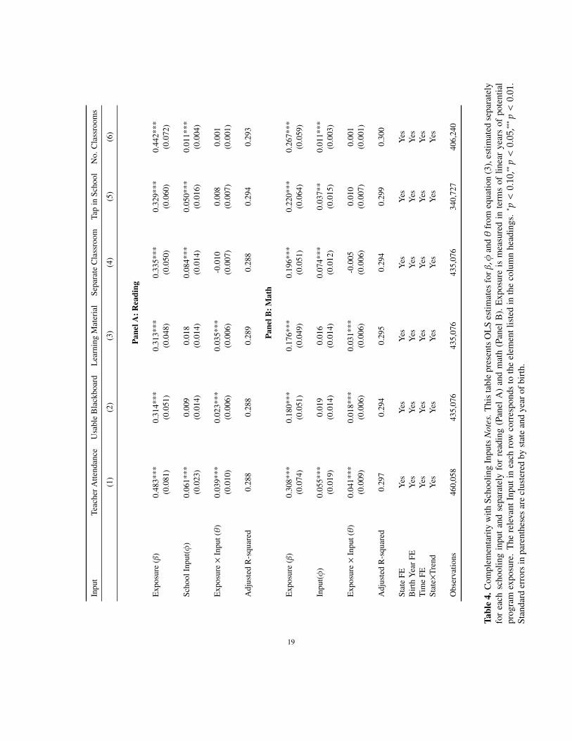
The findings are reported in Table 4, which presents OLS estimates for β, φ and θ from equation (3),estimated separately for each schooling input, separately for reading (Panel A) and math (Panel B).These results are robust to correcting for multiple hypothesis testing; See Online Appendix Table A3.They suggest the presence of significant complementarities with respect to those teaching inputs thatare directly related to learning opportunities of children. For instance in column 1, we see that a 10percentage point increase in teacher attendance is associated with a 0.006 (0.005) point increase inreading (math) scores on its own. However, when combined with one additional year of exposure toschool lunches, a 10 percentage point increase in teacher attendance is associated with a roughly 0.01point increase in reading and math scores. Although access to a functional blackboard (column 2) orsupplementary learning material (column 3) don’t by themselves improve test scores, when combinedwith midday meals they improve both reading and math test performance.

By contrast, in columns 4-6 we see that more general schooling infrastructure like the availabilityof separate classrooms, access to drinking water tap, or the total number of classrooms, is not com-plementary to midday meals. Together these results suggest that schooling inputs that are used inclassroom instruction are complements to midday meals, but more general schooling infrastructure isnot. What we interpret as complementarity may, however, be a reflection of differential funding for,and quality of, program implementation. More specifically, it is possible that early implementers arealso states that have also more generously invested in midday meals and other schooling inputs. Thisseems unlikely given the anecdotal evidence discussed in Section 2. Furthermore, as we will see inSection 6.6, baseline program effects are not affected by the inclusion of schooling inputs as controls.Nevertheless, we cannot rule this out in the absence of state-level funding information.

5.2. Heterogeneous Treatment Effects. The efficacy of school feeding programs in improvinglearning achievement depends on whether they improve attendance and nutrition, and whether thistranslates into better school performance. On the one hand, there are a couple of related reasonswhy disadvantaged children may derive greater benefit from the program’s nutritional benefits thanmore privileged children. First, as Afridi (2010) has documented, midday meals are more likely toincrease the nutritional intake of disadvantaged children. Second, since poorer children start from alower nutritional baseline, the marginal benefits of improved nutrition are likely to be larger for themthan for more privileged children who tend to have better nutritional status; see Strauss and Thomas(1998) and Strauss (1986) who document an increasing concave relationship between nutrition andproductivity. On the other hand, disadvantaged children may be less well positioned to take advantageof these nutritional benefits because they face larger barriers to (regular) school attendance.

Figure 4 investigates the presence of heterogeneous treatment effects for reading scores along twodimensions, namely, gender and housing assets; analogous results for math scores are presented inOnline Appendix Figure A5. Female disadvantage in terms of educational outcomes has been well-documented for India; see for example, Kingdon (2002, 2007). Following the logic outlined above,we would expect baseline test performance to be lower for girls than for boys, but for girls to bemore responsive to program exposure. The focus of the ASER survey is on testing children, and asa consequence information on economic status is rudimentary. Still, enumerators do record someproxies for wealth for the years 2008-2012, the most complete of which is housing assets.24 This

24Patterns are similar for other measures of economic status, such as a broader asset index constructed using princi-pal components analysis. However, reduced sample sizes due to missing observations on these indicators preclude thecalculation of confidence intervals for marginal effects.

20

11.

52

2.5

3P

redi

cted

Rea

ding

Sco

re

0-1 1-2 2-3 3-4 4-5Years of Potential Program Exposure

MaleFemale

(a) Gender

11.

52

2.5

3P

redi

cted

Rea

ding

Sco

re

0-1 1-2 2-3 3-4 4-5Years of Potential Program Exposure

KatchaSemipuccaPucca

(b) Housing

Figure 4. Heterogeneous Responses: Reading. Notes: This graph depicts predicted reading test scoresfor different years of potential exposure by gender (panel a) and housing assets (panel b). Bars denote95% confidence intervals, with standard errors clustered by state and time.

comprises a record of the material from which a house is made, where “Pucca” denotes a house madeof durable materials such as brick, stones or cement; “Kutcha” denotes a house made of less durablematerials such as mud, reeds, or bamboo; and “Semipucca” denotes something in between. Hence,Pucca (Kutcha) is a proxy for relatively high (low) economic status. Here again, we expect thatchildren living in Pucca houses have better baseline performance than children living in poorer qualityhousing, but that the increase in test scores with exposure is larger for the latter, more disadvantaged,group relative to the wealthier former group.

Figure 4 shows that our first prior is confirmed: girls perform worse than boys, as do poorer children(those living in Semipucca or Kutcha housing) relative to wealthier children. However, there is noevidence that disadvantaged children enjoy higher marginal benefits from program exposure. This“negative” result is likely to reflect three realities. First, these are crude measures of disadvantagecompared to measures like consumption expenditure or (better yet) baseline caloric intake; this maymask differences in marginal effects of program exposure. Second, these children are starting froma very low baseline in terms of nutritional status. Deaton and Dreze (2009) report that three quar-ters of the Indian population lives in households whose per capita calorie consumption lies below“minimum requirements” and that even privileged Indian children are mildly stunted. It is possible,in this context, that marginal effects of nutritional input are high, and roughly comparable, for bothrelatively privileged and relatively disadvantaged children. Finally, these children may not be able toreap potential nutritional benefits of the program because they are unable to attend school with anyregularity.

21

Rea

ding

Mat

h

Full

Sam

ple

Full

Sam

ple

Full

Sam

ple

Fem

ale

Onl

yFu

llSa

mpl

eFu

llSa

mpl

eFu

llSa

mpl

eFe

mal

eO

nly

R=

HH

Size

Atl

east

Sibl

ing

Mal

eH

HSi

zeA

tlea

stSi

blin

gM

ale

1si

blin

gw

ithou

tMD

Msi

blin

g1

sibl

ing

with

outM

DM

sibl

ing

(1)

(2)

(3)

(4)

(5)

(6)

(7)

(8)

Exp

osur

e(β

)0.

076*

**0.

069*

**0.

083*

**0.

070*

**0.

044*

*0.

038*

*0.

050*

**0.

041*

*(0

.016

)(0

.016

)(0

.015

)(0

.016

)(0

.018

)(0

.018

)(0

.017

)(0

.017

)In

tera

ctio

nE

ffec

tsR×

Exp

osur

e-0

.002

***

-0.0

06-0

.036

***

-0.0

10**

*-0

.002

***

-0.0

04-0

.029

***

-0.0

05(0

.001

)(0

.005

)(0

.004

)(0

.004

)(0

.000

)(0

.005

)(0

.003

)(0

.003

)

Lev

elE

ffec

tsR

-0.0

00-0

.059

***

0.05

4***

0.03

6***

-0.0

01-0

.044

***

0.05

4***

0.04

4***

(0.0

01)

(0.0

14)

(0.0

10)

(0.0

07)

(0.0

01)

(0.0

13)

(0.0

09)

(0.0

07)

Tota

lSib

lings

-0.0

34**

*-0

.035

***

-0.0

30**

*-0

.030

***

(0.0

03)

(0.0

03)

(0.0

03)

(0.0

03)

F-Te

st:P

-val

ue0.

990.

990.

990.

990.

990.

990.

940.

99

Obs

erva

tions

1,22

2,41

51,

238,

781

1,23

8,78

157

8,17

71,

222,

415

1,23

8,78

11,

238,

781

578,

177

Adj

uste

dR

-squ

ared

0.27

40.

273

0.27

50.

273

0.26

50.

264

0.26

60.

263

Tabl

e5.

Intr

a-ho

useh

old

Red

istr

ibut

ion

Not

es.

Thi

sta

ble

pres

ents

estim

ates

from

anin

tera

ctio

nof

year

sof

polic

yex

posu

rew

ithva

riou

sin

dica

tors

ofth

epo

tent

ialf

orin

tra-

hous

ehol

dre

dist

ribu

tion.

Exp

osur

eis

mea

sure

din

term

sofl

inea

ryea

rsof

pote

ntia

lpro

gram

expo

sure

.All

spec

ifica

tions

incl

ude

stat

e,bi

rth

year

,an

dtim

efix

edef

fect

san

da

stat

e-le

vell

inea

rtim

etr

end.

MD

Mst

ands

form

idda

ym

eal.

Rep

orte

dP-

valu

esar

efr

oman

F-te

stof

whe

ther

the

effe

ctof

Exp

osur

eis

posi

tive

fort

here

spec

tive

inte

ract

ion

vari

able

.Fo

rhou

seho

ldsi

ze,t

heef

fect

isev

alua

ted

atth

em

ean

valu

eof

hous

ehol

dsi

ze.∗p<

0.10,∗∗

p<

0.05,∗∗∗p<

0.01

.St

anda

rder

rors

inpa

rent

hese

sar

ecl

uste

red

byst

ate

and

year

ofbi

rth.

22

5.3. Intra-Household Redistribution. Our implicit assumption throughout this paper has been thatmidday meals improve the nutritional status of children directly exposed to the program. But this isnot self-evident. Although midday meals are targeted in-kind transfers, intrahousehold redistributionaway from the targeted child towards other family members may temper the program’s effect onlearning; see, for example, Das et al. (2013). The extent to which this takes place depends, amongother things, on parental preferences and family composition. Redistribution may be triggered byadditional children in the household, traditional son-preference, or simply by having more mouths tofeed.

Table 5 investigates these possibilities. The first row confirms our baseline results that each additionalyear of exposure to the program improves test scores significantly. The negative coefficient on theinteraction term in columns 1 and 5 suggests that children living in larger households experiencesmaller improvements in reading scores for additional years of exposure to the program compared tochildren living in smaller households. However, the marginal effect of one additional member in thehousehold is close to zero. It is, of course, conceivable that when redistribution occurs it takes placeacross children and not from children to adults. This possibility is explored in columns 2 and 6 bycomparing children with and without any siblings. We do not find any evidence of redistribution toother children in the household.

The implicit assumption in columns 2 and 6 is that households do not distinguish between additionalchildren based on their eligibility for midday meals in school. However, the need for redistributionacross children is likely to arise only when the household budget constraint binds. Additional siblingslead to fewer resources per child in the household only when they are not eligible for midday meals.On the other hand, siblings eligible for free meals in school are likely to relax the household budgetconstraint. Columns 3 and 7 explore this by comparing children who have the same number ofsiblings but vary in terms of their siblings’ eligibility for midday meals in school. We categorizesiblings as non-eligible for school lunches either if they are too young to be in school or if theyhave already completed primary school. The coefficients indicates that children who have siblingsreceiving midday meals in school experience a 0.08 (0.05) point increase in reading (math) scoresfor each additional year of policy exposure. However, for a child with siblings who do not receivefree meals in school, the reading or math score goes up only by half that amount. This suggeststhe presence of partial intra-household redistribution away from the child receiving midday meals inschool to the child not eligible for midday meals in school.

Finally, we investigate intra-household redistribution against the backdrop of a well-known male biasin Indian households. Columns 4 and 8 compare the effect of program exposure on female childrenwith and without male siblings. Our prior here is that in the presence of an inherent male bias,parents are more likely to spend the additional resources freed up on the male sibling. However,the coefficient estimate, although negative, is small relative to the level effect of the exposure and isstatistically significant only in the case of reading. This points to negligible redistribution.

Overall, we find some evidence of substitution away from potential midday meal recipients. How-ever, even in situations where substitution exists, redistribution is only partial so that, in general, thebenefits from the school meals tend to stick to the targeted child.

23

6. ROBUSTNESS

In this section we show that our main results from Section 4 are robust to a number of specificationchecks. Although the findings in this section generally hold for a quadratic specification as well, wekeep things simple by estimating β using OLS in the following linear specification where exposure ismeasured in months:

(4) yitcs = α + β · Exposurei(tcs) + δt + δc + δs + γst + εi

The estimates we present in this section are therefore directly comparable to those in columns 2and 6 of Table 3 for reading and math, respectively. Section 6.1 deals with test score measurementissues. Section 6.2, demonstrates that a “treatment effect” is absent for a placebo group of secondary-school-aged children who were presumably not exposed to the program. Section 6.3 shows that theresults are not driven by cohort-specific performance within states. In Section 6.4, we provide furtherevidence that our results are not driven by differences in the timing of implementation. Finally, inSection 6.6, we show that our results are robust to the inclusion of contemporaneous changes in otherschooling inputs.

Table 7 presents estimates for β in equation (4) for these specification tests, with minor variations, aswe will explain where relevant. The remainder of this section discusses these robustness checks andtheir results in more detail.

6.1. Test Score Measurement. In this section, we address two measurement issues pertaining to theoutcome variable. The first is that we have treated test scores as interval scales, when in fact theyare ordinal variables. The second is that there was a change in the number of levels of attainmentcaptured in the test between the first couple of survey years and later survey years. We deal with eachof these in turn.

ASER’s tests comprise 5 levels, which represent cumulative skill mastery. For both tests separately,the child is marked at the highest level he or she can do comfortably. The first measurement issuearises from the fact that we have assigned integer values (0,1,2,3 or 4) to these levels. In so doing, weare treating test scores as interval scales, when in fact, they have an ordinal scale. This is problematicfor two reasons. First, comparisons across groups—in our case children with different lengths ofprogram exposure—are sensitive to the choice of scale. Second, interpretation of treatment effectsare tricky in this context: with an ordinal scale, it is hard to know which levels of learning achievementare driving the percentage improvement over the baseline test scores.25

Table 6 addresses the ordinality of the test score measure by estimating linear probability modelsin which the dependent variable is a dummy variable equal to 1 if the child has achieved at least acertain level of mastery—separately for levels 1, 2, 3 and 4—in reading (Panel A) and math (Panel B).It confirms our main result that increased exposure fosters learning achievement. Furthermore, theestimates provide a useful interpretation of the effect of midday meal exposure on learning. Childrenwith the full five years of exposure are not significantly more likely to move from having no masteryat all to at least basic knowledge of either reading (word recognition or better) or math (one-digit

25See Bond and Lang (2013) for a clear exposition of these issues and Singh (2017) for a nice application in a developingcountry context.

24

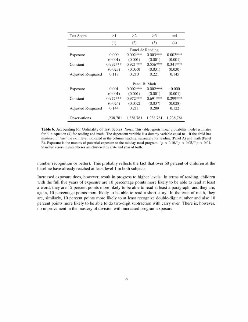
Test Score ≥1 ≥2 ≥3 =4

(1) (2) (3) (4)

Panel A: ReadingExposure 0.000 0.002*** 0.003*** 0.002***

(0.001) (0.001) (0.001) (0.001)Constant 0.992*** 0.921*** 0.556*** 0.341***

(0.023) (0.030) (0.031) (0.030)Adjusted R-squared 0.118 0.210 0.221 0.145

Panel B: MathExposure 0.001 0.002*** 0.002*** -0.000

(0.001) (0.001) (0.001) (0.001)Constant 0.972*** 0.972*** 0.691*** 0.299***

(0.024) (0.032) (0.037) (0.028)Adjusted R-squared 0.144 0.211 0.209 0.122

Observations 1,238,781 1,238,781 1,238,781 1,238,781

Table 6. Accounting for Ordinality of Test Scores. Notes. This table reports linear probability model estimatesfor β in equation (4) for reading and math. The dependent variable is a dummy variable equal to 1 if the child hasmastered at least the skill level indicated in the column heading, separately for reading (Panel A) and math (PanelB). Exposure is the months of potential exposure to the midday meal program. ∗p < 0.10,∗∗ p < 0.05,∗∗∗ p < 0.01.Standard errors in parentheses are clustered by state and year of birth.

number recognition or better). This probably reflects the fact that over 60 percent of children at thebaseline have already reached at least level 1 in both subjects.

Increased exposure does, however, result in progress to higher levels. In terms of reading, childrenwith the full five years of exposure are 10 percentage points more likely to be able to read at leasta word; they are 15 percent points more likely to be able to read at least a paragraph; and they are,again, 10 percentage points more likely to be able to read a short story. In the case of math, theyare, similarly, 10 percent points more likely to at least recognize double-digit number and also 10percent points more likely to be able to do two-digit subtraction with carry over. There is, however,no improvement in the mastery of division with increased program exposure.

25

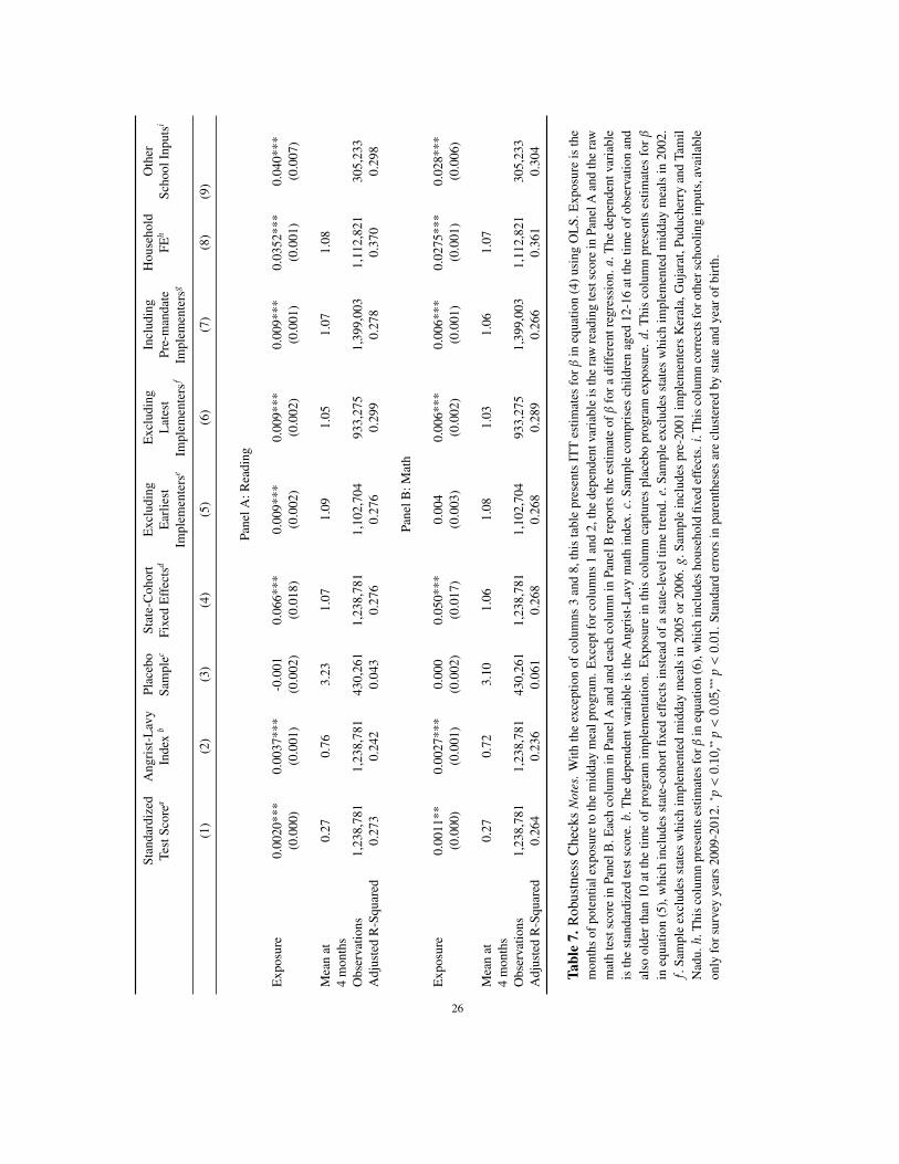
Stan

dard

ized

Ang

rist

-Lav

yPl

aceb

oSt

ate-

Coh

ort

Exc

ludi

ngE

xclu

ding

Incl

udin

gH

ouse

hold

Oth

erTe

stSc

orea

Inde

xb

Sam

plec

Fixe

dE

ffec

tsd

Ear

liest

Lat

est

Pre-

man

date

FEh

Scho

olIn

puts

i

Impl

emen

ters

eIm

plem

ente

rsf

Impl

emen

ters

g

(1)

(2)

(3)

(4)

(5)

(6)

(7)

(8)

(9)

Pane

lA:R

eadi

ng

Exp

osur

e0.

0020

***

0.00

37**

*-0

.001

0.06

6***

0.00

9***

0.00

9***

0.00

9***

0.03

52**

*0.

040*

**(0

.000

)(0

.001

)(0

.002

)(0

.018

)(0

.002

)(0

.002

)(0

.001

)(0

.001

)(0

.007

)

Mea

nat

0.27

0.76

3.23

1.07

1.09

1.05

1.07

1.08

4m

onth

sO

bser

vatio

ns1,

238,

781

1,23

8,78

143

0,26

11,

238,

781

1,10

2,70

493

3,27

51,

399,

003

1,11

2,82

130

5,23

3A

djus

ted

R-S

quar

ed0.

273

0.24

20.

043

0.27

60.

276

0.29

90.

278

0.37

00.

298

Pane

lB:M

ath

Exp

osur

e0.

0011

**0.

0027

***

0.00

00.

050*

**0.

004

0.00

6***

0.00

6***

0.02

75**

*0.

028*

**(0

.000

)(0

.001

)(0

.002

)(0

.017

)(0

.003

)(0

.002

)(0

.001

)(0

.001

)(0

.006

)

Mea

nat

0.27

0.72

3.10

1.06

1.08

1.03

1.06

1.07

4m

onth

sO

bser

vatio

ns1,

238,

781

1,23

8,78

143

0,26

11,

238,

781

1,10

2,70

493

3,27

51,

399,

003

1,11

2,82

130

5,23

3A

djus

ted

R-S

quar

ed0.

264

0.23

60.

061

0.26

80.

268

0.28

90.

266

0.36

10.

304

Tabl

e7.

Rob

ustn

ess

Che

cks

Not

es.W

ithth

eex

cept

ion

ofco

lum

ns3

and

8,th

ista

ble

pres

ents

ITT

estim

ates

forβ

ineq

uatio

n(4

)usi

ngO

LS.

Exp

osur

eis

the

mon

ths

ofpo

tent

iale

xpos

ure

toth

em

idda

ym

ealp

rogr

am.E

xcep

tfor

colu

mns

1an

d2,

the

depe

nden

tvar

iabl

eis

the

raw

read

ing

test

scor

ein

Pane

lAan

dth

era

wm

ath

test

scor

ein

Pane

lB.E

ach

colu

mn

inPa

nelA

and

and

each

colu

mn

inPa

nelB

repo

rts

the

estim

ate

ofβ

fora

diff

eren

treg

ress

ion.

a.T

hede

pend

entv

aria

ble

isth

est

anda

rdiz

edte

stsc

ore.

b.T

hede

pend

entv

aria

ble

isth

eA

ngri

st-L

avy

mat

hin

dex.

c.Sa

mpl

eco

mpr

ises

child

ren

aged

12-1

6at

the

time

ofob

serv

atio

nan

dal

sool

der

than

10at

the

time

ofpr

ogra

mim

plem

enta

tion.

Exp

osur

ein

this

colu

mn

capt

ures

plac

ebo

prog

ram

expo

sure

.d.

Thi

sco

lum

npr

esen

tses

timat

esfo

rβ

ineq

uatio

n(5

),w

hich

incl

udes

stat

e-co

hort

fixed

effe

cts

inst

ead

ofa

stat

e-le

velt

ime

tren

d.e.

Sam

ple

excl

udes

stat

esw

hich

impl

emen

ted

mid

day

mea

lsin

2002

.f.

Sam

ple

excl

udes

stat

esw

hich

impl

emen

ted

mid

day

mea

lsin

2005

or20

06.

g.Sa

mpl

ein

clud

espr

e-20

01im

plem

ente

rsK

eral

a,G

ujar

at,P

uduc

herr

yan

dTa

mil

Nad

u.h.

Thi

sco

lum

npr

esen

tses

timat

esfo

rβin

equa

tion

(6),

whi

chin

clud

esho

useh

old

fixed

effe

cts.

i.T

his

colu

mn

corr

ects

foro

ther

scho

olin

gin

puts

,ava

ilabl

eon

lyfo

rsur

vey

year

s20

09-2

012.∗p<

0.10,∗∗

p<

0.05,∗∗∗p<

0.01

.Sta

ndar

der

rors

inpa

rent

hese

sar

ecl

uste

red

byst

ate

and

year

ofbi

rth.

26

The second measurement issue arises from a change in the test instrument. From 2007-2012, testscores took 5 integer values: 0, 1, 2, 3 and 4. In 2005 and 2006, however, ASER aggregated singleand double digit number recognition, so math test scores took on only 4 values. In our preferredspecification, we use these raw test scores as outcome variables for the ease of interpreting our results.Due to the lack of disaggregation in the early rounds, we have coded single or double digit masteryin 2005 and 2006 as a math test score equal to 2, so our data contain no math test score values equalto 1 in those two years. This means that average test scores are mechanically higher in the first twosurvey years than in later survey years26. Survey year fixed effects will pick up these differences inpart. Here we account for this change in measurement by standardizing the test scores in two ways:first, through z-scores, and second by constructing Angrist-Lavy Indices following Angrist and Lavy(1997). The z-scores are constructed in the usual manner, by standardizing the test score separatelyfor each survey year. The Angrist-Lavy measure takes this standardized test score and assigns theindex a value 0 if the standardized score is 0, a value 1 if it is less than or equal to one-half, and avalue 2 if it is greater than one-half.

Table 7 presents estimates for β in equation (4) with the dependent variable being standardized testscores in column 1 and the Angrist-Lavy index in column 2. The results are qualitatively identical toour main results, indicating that the change in math assessment scoring is not material to our mainresult.

6.2. Placebo. In this section, we present estimates for equation (4) on the set of children aged 12-16at the time of the survey; and who were also 11 or older—above the primary school going age—atthe time of midday meals implementation. This constitutes a placebo group, which was potentiallyunexposed to the program.27 In an exercise similar to the construction of potential years of exposure,we assign pseudo years of exposure to these older children. Specifically, pseudo years of exposurefor children of age 12 at the time of the survey would be the same as the years of actual exposureassigned to children of age 6 according to the Online Appendix Table B1. The Exposure variable inthe table reflects this placebo exposure.

We expect a null result: since these children were potentially not exposed to the program, our ITTestimate β on this placebo exposure should be statistically insignificant and close to zero. This isconfirmed in column 3 of Table 7. The result also lends support to the underlying assumption ofparallel-trends in our estimation strategy.

6.3. State-cohort Specific Effects. In this section, we tackle the concern that the timing of programimplementation is correlated with cohort-specific performance within states, by introducing cohort-state fixed effects. Column 4 of Table 7 presents estimates for β in the following regression:

(5) yitcs = α + β · Exposurei(tcs) + δt + δc + δs + γcs + εi

26In an alternate measure, we aggregated the math scores in 2007-2012, recoding double digit mastery in 2007-2012 asa math test score equal to 1. This alternate measure has 4 overall categories and a mechanically lower average test score inthe later years. The results using this alternate measure are very similar in spirit to the ones we obtain in Table3.

27We say “potentially unexposed” because it is possible that some schools in some states also introduced midday mealsto this group. In some cases the states voluntarily extended the program to secondary schools prior to this; others did solater, or not at all. Clear documentation on implementation of the secondary school meals program does not exist. Theupper bound on this age group is restricted by the data availability as ASER only tested children up to the age of 16.

27

As we explained in Section 3.2, variation in exposure is jointly determined by a child’s age at thetime of program implementation, and their age at the time of observation. Both depend on the child’sbirth cohort. For a given birth cohort, the latter depends on the survey year; the former depends on thetiming of implementation in the child’s state. With state-cohort fixed effects, variation in the exposurevariable comes from observing the same cohort in a given state over consecutive survey years, as thechild progresses through primary school grades. The admittedly strong identifying assumption inthis context, is non-linearity in learning achievement within a state-cohort, as it progresses throughconsecutive grades.

The estimates in column 4 are bigger than our main results in columns 2 and 6 of Table 3. Thissuggests that failing to account for state-cohort effects, if anything, may result in underestimation ofthe true effects of midday meal exposure.

6.4. Timing. Columns 5-7 of Table 7 explore to what extent the timing of implementation influencesour result by considering alternative samples based on the date of program implementation. Column5 excludes states who were the earliest (2002) implementers. Column 6 excludes the late (2005-2006)implementers. Column 7 includes Kerala, Gujarat, Puducherry and Tamil Nadu, which had middaymeals in place prior to the 2001 Supreme Court Mandate. In one specification the estimate for mathscores is imprecise, but in general the estimates are statistically significant and their magnitudes arevery similar to those in our main results. Finally, dropping states one-by-one does not affect theresults either, indicating that our findings do not hinge on any one state (results not shown.)

6.5. Household Fixed Effects. The main results in this paper neglect the possibility that there maybe unobserved heterogeneity at the family level. More specifically, it is plausible that children frombetter-off families have higher test scores, and do not suffer nutritional disadvantage, resulting in adownward bias in the treatment effect of exposure. We account for this by estimating the followinghousehold fixed effects model:

(6) yihtcs = β · Exposurei(tcs) + δh(i) + δc + γst + εi

where δh(i) is a household fixed effect of child i living in household h, and the remaining parametersare defined as before. Identification of β in this specification exploits variation in exposure acrossdifferent children in the same household. Column 8 of Table 7 presents the results. They suggestthat, indeed, the estimates in Table 3 may be downward biased estimates of the true treatment effect.The treatment effects estimated with household fixed effects remain statistically significant at the 1percent level and are 4-6 times as large as the analogous OLS estimates.

6.6. Other Schooling Inputs. One concern with our quasi-experiment design is the possibility ofsimultaneous changes in schooling inputs other than midday meals. We account for this in Column9 of Table 7, by controlling for a range of schooling inputs that could be spuriously correlated withmidday meal exposure. These controls include teacher attendance; the availability of usable black-boards and the availability of supplementary learning material in school; whether different grades aretaught in different classrooms; the total number of usable classrooms; and access to a functional tapfor drinking water. As explained in Section 5.1, including these school-level controls entails a consid-erable loss in sample size since comprehensive school surveys were only conducted from 2009-2012.

28

As a result, the coefficient estimates in Column 9 are not directly comparable to those in Table 3.Table A4 in the Online Appendix provides estimates for each of the controls and elaborates on theramifications of sample loss for the (much larger) point estimates. Here we simply note that the coef-ficient on program exposure remains positive and statistically significance, even after controlling forother schooling inputs.

7. CONCLUSION

This paper has explored the effect of school feeding programs on children’s learning achievement.What sets it apart from previous papers is that it studies the effect of long-term program exposure, toa large-scale program, using a large data set. The results indicate that exposure to midday meals forthe nearly five-year duration of primary school increases test scores by 18% (0.17σ) for reading and9% (0.09σ) for math relative to children with less than a year of exposure.

We show that there are complementarities between teaching- and learning-related classroom inputs,though not with more general schooling infrastructure. Relatively disadvantaged children show nodifferential treatment response, probably because the children in this rural Indian sample may havelow baseline nutrition to begin with. And there is some evidence of partial redistribution away fromprogram recipients but, in general, this in-kind transfer tends to “stick” to its intended beneficiaries.

While the focus of this paper has been on the learning effect of midday meals it is worth rememberingthat this is, if anything, a side benefit of the program. Its primary aim was to improve child nutrition,and available evidence suggests that it has been quite successful in so doing. For example, in a carefulstudy, Afridi (2010) finds that the program reduced primary school children’s daily deficiencies inprotein, caloric intake and iron by roughly 100%, 30% and 10%, respectively. In keeping with thetheme of this paper, the remainder of this section will discuss the cost effectiveness of this programwhen it comes to learning outcomes. This means that while the costs we describe cover the marginalcost of what is effectively a child nutrition program, the benefits we will describe pertain solely to thelearning improvements; as such, the latter may be considered a lower bound on the “true” benefits ofthe program, which are likely to include both nutrition and health, in addition to learning.

One way to understand the cost effectiveness of the midday meals program with respect to learningoutcomes is to compare it with alternative education interventions that target test score improvements.In principle, improving test scores can be accomplished by enhancing any number of schooling in-puts including teacher quality, teacher numbers, teacher attendance or teaching aids. A few recentpapers in the Indian context have studied the effect on test scores of improvements in the pupil-teacher-ratio (Muralidharan and Sundararaman, 2013), additional instruction through private tutoring(Banerjee et al., 2007; Berry and Mukherjee, 2016) and additional instruction through technology-aided methods (Muralidharan et al., 2016; Banerjee et al., 2007). Of these, Banerjee et al. (2007)and Muralidharan and Sundararaman (2013) provide contexts which are most closely comparable toours in that their focus is also on primary school children. Hence, in what follows we use these twostudies as benchmarks against which to compare the costs and learning benefits of the midday mealprogram.

Banerjee et al. (2007) study the effect of tutoring outside the classroom in the form of two alter-nate interventions. In the first—the “Balsakhi” program—weaker children in third and fourth gradeswere taught for two hours during school time by women from the local community. Effectively, the

29

0.1

.2.3

.4.5

Rea

ding

scor

e im

prov

emen

t (σ

)

12 24 36 48 60Months of Program Exposure

Midday MealBalsakhi

Contract Teacher

(a) Reading

0.1

.2.3

.4.5

Mat

h sc

ore

impr

ovem

ent

(σ)

12 24 36 48 60Months of Program Exposure

Midday MealBalsakhi

Contract Teacher

(b) Math

Figure 5. Benefits of Midday Meals, Balsakhi, and Contract Teachers. Notes: This graph plots the effect ofmidday meal exposure on standardized test scores by month. The y-axis plots the improvement, measured in standarddeviations (σ), in reading scores (panel a) and math scores (panel b). The midday meal program is compared totwo comparable programs aimed at improving test scores, both of which lasted for two years: the Balsakhi program(Banerjee et al., 2007) and contract-teacher program (Muralidharan and Sundararaman, 2013).

program replaced regular classroom teaching by tutoring that involved more personalized attention.The second intervention included two hours of computer assisted learning (CAL) that involved mathsolving games during school time. Muralidharan and Sundararaman (2013) study the effect on testscores of reducing pupil-teacher-ratios in public schools by appointing contract teachers.

Figure 5 provides a graphical comparison of the standard deviation increases in reading scores (Panela) and math scores (Panel b) from midday meal exposure to those of Banerjee et al. (2007)’s Balsakhis(squares) and Muralidharan and Sundararaman (2013)’s contract teachers (triangles).28 The dashedblue line plots the standard deviation changes in test scores for each additional month of midday mealexposure, based on the quadratic “Exposure” estimates in columns 4 and 8 for reading and math,respectively; see Online Appendix Table A6. At the two-year mark the improvement in readingscores for midday meals compares favorably to that resulting from Balsakhi and contract teacherinterventions. For math, improvement in scores from midday meals is substantially lower than thatfrom Balsakhis, but slightly outperforms contract teachers.

Table 8 furnishes a more detailed cost-benefit comparison of these three programs. Columns 2 and4 present the improvement in reading and math test scores, respectively, after two years of programexposure. Columns 3 and 5 present the improvement in test scores per dollar spent after two years ofexposure, based on the annual cost estimates per child per year, presented in column 1. According toour calculations, discussed in Section 2, the cost of midday meal provision is 10 USD per child per

28Muralidharan and Sundararaman (2013) also provides estimates of the effect of reducing pupil-teacher-ratio by hiringpermanent teachers on student achievement. However, these estimates are not comparable to our study since they do notcapture the direct program effect of hiring an additional permanent teacher or the marginal cost of so doing. Hence werestrict our comparison to the contract teacher estimates. Similarly, the training, as part of the CAL program, in Banerjeeet al. (2007), is restricted to numerical skills and effectively do provide comparable estimates of reading scores. Wetherefore do not incorporate CAL estimates in our cost-benefit comparisons either.

30

Program Reading Score Math Score

Annual Costa Benefit Benefit Benefit Benefit(USD) (σ) per USD (σ) per USD

spent spent

(1) (2) (3) (4) (5)

Midday Mealsb 10 0.25 0.013 0.22 0.011Balsakhic 3.5 0.19 0.027 0.35 0.050Contract Teachersd 3.4 0.15 0.022 0.16 0.024

Table 8. Cost Benefit Comparison after Two Years of Program Exposure. Notes. This table reports the annualcost of the program in 2009 USD (column 1); standard deviation improvements (benefit) in test scores (columns 2 &4); and the corresponding improvement in test scores per dollar spent (columns 3 & 5). Note that the latter accountsfor 2 years of costs after two years of program exposure. a. USD costs are calculated by converting nominal IndianRupee amounts to 2009 Indian Rupees using the general CPI for industrial workers and then converting this Rupeeamount to USD using 2009 exchange rates. b. Benefits calculated based on the estimates in columns 4 and 8 of theOnline Appendix Table A6; authors’ cost calculations. c. Balsakhi program estimates from Banerjee et al. (2007).The Balsakhi program cost Rs. 107 per child per year in 2002. d. Contract teacher estimates from Muralidharan andSundararaman (2013); a contract teacher cost of Rs. 1500 per month in 2006-2007. The per child cost was calculatedassuming an average class size of 30 in grades one through four according to the sample in the paper.

year.29 The marginal cost of midday meals is thus almost three times higher than that of Balsakhis orcontract teachers. This likely reflects the fact that meals are an individual-level consumption activitywith commensurate individual-level costs as opposed to teachers, from whom all the children in agiven class jointly benefit.

The numbers in columns 3 and 5 indicate that, at the two year mark, reading scores increase by0.013σ and math scores by 0.011σ for each additional dollar spent on midday meals. The corre-sponding returns to the Balsakhi and contract teacher programs are at least twice as large due to theirconsiderably lower unit costs. In terms of bang for buck in learning outcomes, therefore, it wouldseem that those programs are a better investment. Then again, the aim of the midday meal programwas to improve nutrition and not learning. Viewed in this light, the program’s learning benefits seemrather remarkable.

29Kristjansson et al. (2016) independently comes to the same estimate, and remarks that this makes midday meals oneof the cheapest school feeding programs in the world. Note that 10 USD per child per year is the marginal cost of theprogram which, in the Indian context, rides on (fixed costs of) a well developed Public Distribution System. Marginal costsare likely to be substantially higher in countries which do not have such a system.

31

REFERENCES

Adelman, S., H. Alderman, D. O. Gilligan, and K. Lehrer (2008). The Impact of Alternative Food forEducation Programs on Learning Achievement and Cognitive Development in Northern Uganda.University of Maryland, College Park Working Paper.

Afridi, F. (2010). Child Welfare Programs and Child Nutrition: Evidence from a Mandated SchoolMeal Program in India. Journal of Development Economics 92(2), 152–165.

Afridi, F. (2011). The Impact of School Meals on School Participation: Evidence from Rural India.Journal of Development Studies 47(11), 1636–1656.

Afridi, F., B. Barooah, and R. Somanathan (2014). School Meals and Classroom Attention: Evidencefrom India. Mimeo. Indian Statistical Institute.

Ahmed, A. U. (2004). Impact of Feeding Children in School: Evidence from Bangladesh. Interna-tional Food Policy Research Institute.

Alderman, H. and D. Bundy (2012). School Feeding Programs and Development: Are We Framingthe Question Correctly? The World Bank Research Observer 27(2), 204–221.

Angrist, J. D. and V. Lavy (1997). The Effect of a Change in Language of Instruction on the Returnsto Schooling in Morocco. Journal of Labor Economics 15(1, Part 2), S48–S76.

ASER (2005). Annual Status of Education Report. Technical report, ASER.Banerjee, A. V., S. Cole, E. Duflo, L. Linden, et al. (2007). Remedying Education: Evidence from

Two Randomized Experiments in India. The Quarterly Journal of Economics 122(3), 1235–1264.Behrman, J. R., S. W. Parker, and P. E. Todd (2013). Incentives for Students and Parents, Chapter 5.

University of Chicago Press Chicago, IL.Belot, M. and J. James (2011). Healthy School Meals and Educational Outcomes. Journal of Health

Economics 30(3), 489–504.Berry, J. and P. Mukherjee (2016). Pricing of Private Education in Urban India. Preliminary Results.Bhattacharya, J., J. Currie, and S. J. Haider (2006). Breakfast of Champions? The School Breakfast

Program and the Nutrition of Children and Families. Journal of Human Resources 41(3), 445–466.Bond, T. N. and K. Lang (2013). The Evolution of the Black-White Test Score Gap in Grades K–3:

The Fragility of Results. Review of Economics and Statistics 95(5), 1468–1479.Bundy, D., C. Burbano, M. E. Grosh, A. Gelli, M. Juke, and D. Lesley (2009). Rethinking School

Feeding: Social Safety Nets, Child Development, and the Education Sector. The World Bank.Case, A. and C. Paxson (2008a). Height, Health, and Cognitive Function at Older Ages. American

Economic Review 98(2), 463–467.Case, A. and C. Paxson (2008b). Stature and Status: Height, Ability, and Labor Market Outcomes.

Journal of Political Economy 116(3), 499–532.Centre for Policy Research (2013). Midday Meals Scheme, GOI, 2013-14. Technical report.Das, J., S. Dercon, J. Habyarimana, P. Krishnan, K. Muralidharan, and V. Sundararaman (2013).

School Inputs, Household Substitution, and Test Scores. American Economic Journal: AppliedEconomics 5(2), 29–57.

Deaton, A. and J. Dreze (2009). Food and Nutrition in India: Facts and Interpretations. Economicand Political Weekly Vol. 44(Issue No. 07), 42–65.

Desai, A. H. and S. Muralidhar (2000). Public Interest Litigation: Potential and Problems. Technicalreport. International Environmental Law Research Centre.

Dreze, J. and A. Goyal (2003). Future of Mid-day Meals. Economic and Political Weekly 38(44),4673–4683.

32

Grantham-McGregor, S. M., S. Chang, and S. P. Walker (1998). Evaluation of School Feeding Pro-grams: Some Jamaican Examples. The American Journal of Clinical Nutrition 67(4), 785S–789S.

Jacoby, E. R., S. Cueto, and E. Pollitt (1998). When Science and Politics Listen to Each Other:Good Prospects from a New School Breakfast Program in Peru. The American Journal of ClinicalNutrition 67(4), 795S–797S.

Jacoby, H. G. (2002). Is There an Intrahousehold Flypaper Effect? Evidence from a School FeedingProgramme. The Economic Journal 112(476), 196–221.

Jayaraman, R. and D. Simroth (2015). The Impact of School Lunches on Primary School Enrollment:Evidence from India’s Midday Meal Scheme. The Scandinavian Journal of Economics 17(4),1176–1203.

Jomaa, L. H., E. McDonnell, and C. Probart (2011). School Feeding Programs in Developing Coun-tries: Impacts on Children’s Health and Educational Outcomes. Nutrition Reviews 69(2), 83–98.

Karp, R., R. Martin, T. Sewell, J. Manni, and A. Heller (1992). Growth and Academic Achievementin Inner-City Kindergarten Children: The Relationship of Height, Weight, Cognitive Ability, andNeurodevelopmental Level. Clinical Pediatrics 31(6), 336–340.

Kazianga, H., D. De Walque, and H. Alderman (2012). Educational and Child Labour Impacts of TwoFood-for-Education Schemes: Evidence from a Randomised Trial in Rural Burkina Faso. Journalof African Economies 21(5), 723–760.

King, E. M. and J. R. Behrman (2009). Timing and Duration of Exposure in Evaluations of SocialPrograms. The World Bank Research Observer 24(1), 55–82.

Kingdon, G. G. (2002). The Gender Gap in Educational Attainment in India: How Much Can BeExplained? Journal of Development Studies 39(2), 25–53.

Kingdon, G. G. (2007). The Progress of School Education in India. Oxford Review of EconomicPolicy 23(2), 168–195.

Kremer, M. and C. Vermeersch (2005). School Meals, Educational Achievement, and School Com-petition: Evidence from a Randomized Evaluation. The World Bank.

Kristjansson, E., A. Gelli, V. Welch, T. Greenhalgh, S. Liberato, D. Francis, and F. Espejo (2016).Costs, and Cost-outcome of School Feeding Programmes and Feeding Programmes for YoungChildren. Evidence and Recommendations. International Journal of Educational Development 48,79–83.

Kristjansson, E., V. Robinson, M. Petticrew, B. MacDonald, J. Krasevec, L. Janzen, T. Greenhalgh,G. Wells, J. MacGowan, A. Farmer, et al. (2007). School Feeding for Improving the Physicaland Psychosocial Health of Disadvantaged Elementary School Children. Number 1. CochraneCollaboration.

Lawson, T. M. (2012). Impact of School Feeding Programs on Educational, Nutritional, and Agri-cultural Development Goals: A Systematic Review of Literature. Master’s Thesis.

McEwan, P. J. (2013). The Impact of Chile’s School Feeding Program on Education Outcomes.Economics of Education Review 32, 122–139.

McEwan, P. J. (2015). Improving Learning in Primary Schools of Developing Countries A Meta-Analysis of Randomized Experiments. Review of Educational Research 85(3), 353–394.

MHRD, G. o. I. Documentation on Meal Provision of Midday Meal Scheme. Technical report,Ministry of Human Resource Development, Department of School Education and Literacy, Gov-ernment of India. http://mdm.nic.in, accessed on 24 April, 2016.

Muralidharan, K. (2006). Public-Private Partnerships for Quality Education in India. Mimeo.Muralidharan, K., A. Singh, and A. J. Ganimian (2016). Disrupting Education? Experimental Evi-

dence on Technology-Aided Instruction in India. Technical report, National Bureau of Economic

33

Research Working Paper. No. 22923.Muralidharan, K. and V. Sundararaman (2013). Contract Teachers: Experimental Evidence from

India. Technical report, National Bureau of Economic Research Working Paper. No. 19440.Neumann, C. G., N. O. Bwibo, S. P. Murphy, M. Sigman, S. Whaley, L. H. Allen, D. Guthrie, R. E.

Weiss, and M. W. Demment (2003). Animal Source Foods Improve Dietary Quality, MicronutrientStatus, Growth and Cognitive Function in Kenyan School Children: Background, Study Designand Baseline Findings. The Journal of Nutrition 133(11), 3941S–3949S.

Neumann, C. G., S. P. Murphy, C. Gewa, M. Grillenberger, and N. O. Bwibo (2007). Meat Sup-plementation Improves Growth, Cognitive, and Behavioral Outcomes in Kenyan Children. TheJournal of Nutrition 137(4), 1119–1123.

Powell, C. A., S. P. Walker, S. M. Chang, and S. M. Grantham-McGregor (1998). Nutrition andEducation: A Randomized Rrial of the Effects of Breakfast in Rural Primary School Children. TheAmerican Journal of Clinical Nutrition 68(4), 873–879.

Probe Team (1999). Public Report on Basic Education in India. Oxford University, New Delhi, IN.Schick, A. and R. H. Steckel (2010). Height as a Proxy for Cognitive and Non-Cognitive Ability.

Technical report, National Bureau of Economic Research. No. 16570.Secretariat of the Right to Food Campaign (2005). Midday Meals: A Primer. Right to Food Campaign

Materials.Singh, A. (2008). Do School Meals Work? Treatment Evaluation of the Midday Meal Scheme in

India. Young Lives Mimeo.Singh, A. (2017). Learning More With Every Year: School Year Productivity and International

Learning Divergence. Draft Paper.Singh, A., A. Park, and S. Dercon (2014). School Meals as a Safety Net: An Evaluation of the

Midday Meal Scheme in India. Economic Development and Cultural Change 62(2), 275–306.Spears, D. (2012). Height and Cognitive Achievement among Indian Children. Economics & Human

Biology 10(2), 210–219.Strauss, J. (1986). Does Better Nutrition Raise Farm Productivity? The Journal of Political Econ-

omy 94(2), 297–320.Strauss, J. and D. Thomas (1998). Health, Nutrition, and Economic Development. Journal of Eco-

nomic Literature 36(2), 766–817.Van Stuijvenberg, M. E., J. D. Kvalsvig, M. Faber, M. Kruger, D. G. Kenoyer, and A. S. Benade

(1999). Effect of Iron, Iodine, and β-Carotene–Fortified Biscuits on the Micronutrient Status ofPrimary School Children: A Randomized Controlled Trial. The American Journal of ClinicalNutrition 69(3), 497–503.

WFP (2013). State of School Feeding Worldwide. Technical report, World Food Program. WorldFood Program annual report.

Whaley, S. E., M. Sigman, C. Neumann, N. Bwibo, D. Guthrie, R. E. Weiss, S. Alber, and S. P.Murphy (2003). The Impact of Dietary Intervention on the Cognitive Development of KenyanSchool Children. The Journal of Nutrition 133(11), 3965S–3971S.

34

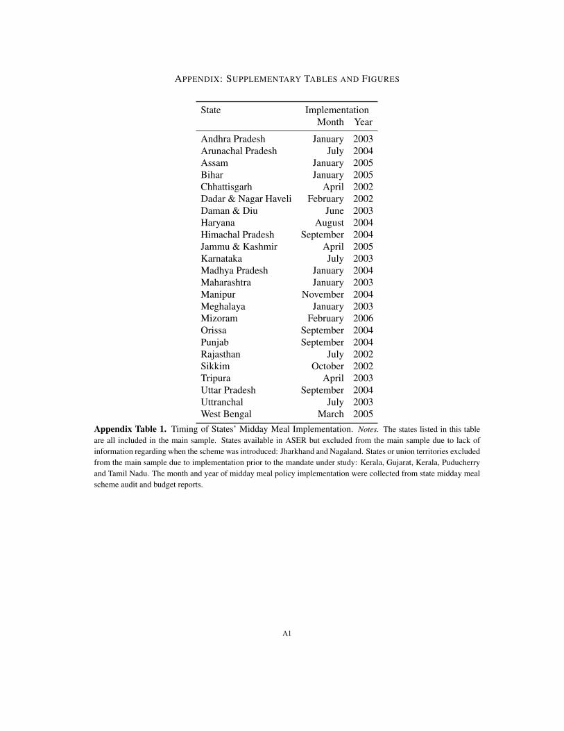
APPENDIX: SUPPLEMENTARY TABLES AND FIGURES

State ImplementationMonth Year

Andhra Pradesh January 2003Arunachal Pradesh July 2004Assam January 2005Bihar January 2005Chhattisgarh April 2002Dadar & Nagar Haveli February 2002Daman & Diu June 2003Haryana August 2004Himachal Pradesh September 2004Jammu & Kashmir April 2005Karnataka July 2003Madhya Pradesh January 2004Maharashtra January 2003Manipur November 2004Meghalaya January 2003Mizoram February 2006Orissa September 2004Punjab September 2004Rajasthan July 2002Sikkim October 2002Tripura April 2003Uttar Pradesh September 2004Uttranchal July 2003West Bengal March 2005

Appendix Table 1. Timing of States’ Midday Meal Implementation. Notes. The states listed in this tableare all included in the main sample. States available in ASER but excluded from the main sample due to lack ofinformation regarding when the scheme was introduced: Jharkhand and Nagaland. States or union territories excludedfrom the main sample due to implementation prior to the mandate under study: Kerala, Gujarat, Kerala, Puducherryand Tamil Nadu. The month and year of midday meal policy implementation were collected from state midday mealscheme audit and budget reports.

A1

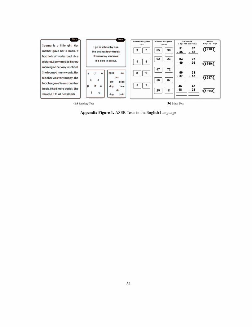
(a) Reading Test (b) Math Test

Appendix Figure 1. ASER Tests in the English Language

A2