Scheme of the equilibrium Environmental Compartments Model

Life-cycle of gaseous contaminants

Processes leading to atmospheric deposition

Dry and wet atmospheric deposition

Wet deposition

Rainout, washout and deposition of aerosols are one-way transport processes that transfer chemicals from the air to water and soils. Most efficient for soluble gases and for aerosols with diameters > 1 µm

Dry deposition

Airborne particles and dry gases

Processes affecting the compositio of rain droplets

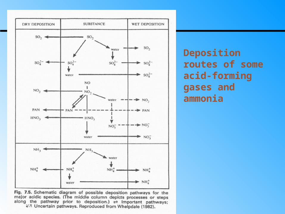
Deposition routes of some acid-forming gases and ammonia

Solubility of gases in liquids

Gas solubility is an equilibrium process controlled by the gas (partial) pressure. At constant temperature, the number of molecules transferred from the gas phase to the liquid phase (solution) is the same as the number of molecules transferred the opposite way. Increasing pressure leads to higher solubility:

Henry’s Law

Distribution of a gas between gas phase (air) and liquid phase (water) is described by the air-water distribution coefficient

Kaw = C(air)/C(aq)where C(air) is the concentration of a chemical in the air and C(aq) its concentration in water. C(air) can be calculated from the equation of state

C(air) = ni/V = pi/RT ni is the number of moles of the chemical in volume V of air and pi is partial pressure of the chemical:

pi = xipwhere p is the (total atmospheric) pressure and xi molar fraction of the chemical in the air. If this chemical is below its critical point and aqueous solution is saturated, i.e. C(aq) = CS, partial pressure is equal to the saturated vapor pressure – pS

More commonly applied is the Henry’s law constant H H = pS / CS = ( pi/C(aq) ) = Kaw RT

Solubility of gases in liquids – example

Calculate the solubility of oxygen in water at 25°C (H = 76900 Pa m3 mol-1)

O2 in air= 20,95 % (molar percentage)

PO2 = 0,2095 patm

C[O2 aq] = pO2 / H

Normal pressure = 105 Pa = 1 bar = 1 atm = 760 mm Hg (torr)(conversion to atm is not exact)

pO2 = 0,2095 105 = 2.095 ·104 Pa

 C[O2 aq] = pO2 /H = 2,7 10–4 mol/l

CT

BAp s

log

Pressure in a closed system containing only pure liquid and gas phases of a given compound is called its (saturated) vapor pressure.

Vapor pressure depends only on temperature. Many empirical correlation equations are used for this relation, most often the

Antoine equation

where A, B, C are constants derived from experimental data and valid only in some limited temperature interval. This equation is usually applied for vapor pressures from 1 to about 200 kPa.

Vapor pressure

Measurements of vapor pressure – static method

H2O (l) H2O (g)

start equilibrium

Phase diagram of water

Factors affecting gas solubility

PressureAccording to Henry’s law, solubility of a gas is proportional to its partial pressure in the air. Because atmospheric pressure is more or less constant, it depends just on the concentration of this gas in the air

Temperature Connected to gas expansivity, i.e. the equation of state: higher temperature leads to more expanded gases and thus lower concentration. Even more important is that Henry’s law constant of gases is growing with temperature. Both effects lead to lower gas solubility

SaltsGases are „salted-out“ from the solution: higher salinity leads to lower gas solubility

Chemical reactions in waterIf the gas is reacting with water, its solubility is increased

Oxygen in the air

Oxygen equilibrium is attained on one side by de-oxygenation (aerobic processes of biochemical degradation of organic compounds) and on the other side by re-aeration (dissolution of oxygen from the air, if water is less than saturated). Equilibrium amount of dissolved oxygen depends on temperature.

Equilibrium concentration of aqueous oxygen vs. temperature (mg/l)

t(°C) 0 10 15 20 25 30

O2(mg/l) 14.6 11.3 10.1 9.2 8.3 7.6

Concentrations below 4 mg/l are lethal to fish and other water organisms

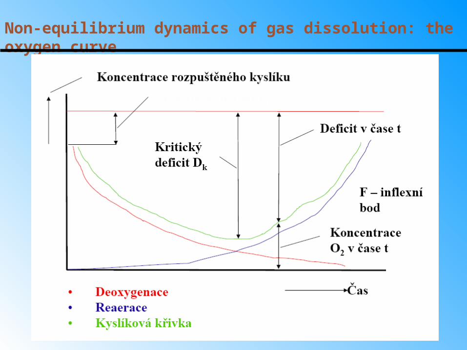
Non-equilibrium dynamics of gas dissolution: the oxygen curve

Re-aeration processes

The rate of oxygen dissolution depends on the water surface quality:

Still water dissolves 1.4 mg O2 per m2 / day

Stirred water dissolves 5.5 mg O2 per m2 / day

Turbulent water dissolves 50 mg O2 per m2 / day

The rate of re-aeration exponentially depends on the oxygen deficit – the above numbers refer to stationary state. Oxygen deficit can be increased by sudden increase of contamination and/or by increased temperature.