scheduling streaming applications on a complex multicore

HAL Id: ensl-00523018https://hal-ens-lyon.archives-ouvertes.fr/ensl-00523018

Preprint submitted on 4 Oct 2010

HAL is a multi-disciplinary open accessarchive for the deposit and dissemination of sci-entific research documents, whether they are pub-lished or not. The documents may come fromteaching and research institutions in France orabroad, or from public or private research centers.

L’archive ouverte pluridisciplinaire HAL, estdestinée au dépôt et à la diffusion de documentsscientifiques de niveau recherche, publiés ou non,émanant des établissements d’enseignement et derecherche français ou étrangers, des laboratoirespublics ou privés.

Scheduling streaming applications on a complexmulticore platform

Tudor David, Mathias Jacquelin, Loris Marchal

To cite this version:Tudor David, Mathias Jacquelin, Loris Marchal. Scheduling streaming applications on a complexmulticore platform. 2010. �ensl-00523018�

https://hal-ens-lyon.archives-ouvertes.fr/ensl-00523018

https://hal.archives-ouvertes.fr

Laboratoire de l’Informatique du Parallélisme

École Normale Supérieure de Lyon

Unité Mixte de Recherche CNRS-INRIA-ENS LYON-UCBL no 5668

Scheduling streaming applications

on a complex multicore platform

Tudor David,Mathias Jacquelin,Loris Marchal

July 2010

Research Report No 2010-25

École Normale Supérieure de Lyon46 Allée d’Italie, 69364 Lyon Cedex 07, France

Téléphone : +33(0)4.72.72.80.37Télécopieur : +33(0)4.72.72.80.80

Adresse électronique : [email protected]

Scheduling streaming applicationson a complex multicore platform

Tudor David, Mathias Jacquelin, Loris Marchal

July 2010

AbstractIn this report, we consider the problem of scheduling streaming applicationsdescribed by complex task graphs on a heterogeneous multi-core platform, theIBM QS 22 platform, embedding two STI Cell BE processor. We first de-rive a complete computation and communication model of the platform, basedon comprehensive benchmarks. Then, we use this model to express the prob-lem of maximizing the throughput of a streaming application on this platform.Although the problem is proven NP-complete, we present an optimal solu-tion based on mixed linear programming. We also propose simpler schedulingheuristics to compute mapping of the application task-graph on the platform.We then come back to the platform, and propose a scheduling software to de-ploy streaming applications on this platform. This allows us to thoroughly testour scheduling strategies on the real platform. We thus show that we are able toachieve a good speed-up, either with the mixed linear programming solution,or using involved scheduling heuristics.

Keywords: Scheduling, multicore processor, streaming application, Cell processor.

RésuméDans ce rapport, nous nous intéressons au problème de l’ordonnancementd’une application de flux décrite par un graphe de tâche sur une plate-formemulti-cœur hétérogène, le QS 22 d’IBM, qui embarque deux processeurs Cell.Nous mettons d’abord au point un modèle de calcul et de communication com-plet de la plate-forme, en nous fondant sur des tests de performances extensifs.Ensuite, nous utilisons ce modèle pour exprimer le problème d’optimisationdu débit d’une application de flux sur cette plate-forme. Nous montrons que ceproblème est NP-complet, et présentons une solution optimale utilisant la pro-grammation linéaire mixte. Nous proposons ensuite des heuristiques de pla-cement plus simples pour déterminer comment distribuer les tâches de l’ap-plication sur la plate-forme. Nous présentons également un canevas logicielpour exécuter une telle application sur cette plate-forme, qui permet de tes-ter les différentes stratégies de placement proposées. Nous montrons ainsi quenous sommes capables d’atteindre des performances intéressantes, soit avecla stratégie utilisant la programmation linéaire, soit avec des heuristiques deplacement élaborées.

Mots-clés: Ordonnancement, processeur multi-cœur, application de flux, processeur Cell.

Scheduling complex streaming applications on a complex multicore platform 1

1 Introduction

The last decade has seen the arrival of multi-core processors in every computer and electronic device,from the personal computer to the high-performance computing cluster. Nowadays, heterogeneousmulti-core processor are emerging. Future processors are likely to embed several special-purposecores –like networking or graphic cores– together with general cores, in order to tackle problems likeheat dissipation, computing capacity or power consumption. Deploying an application on this kind ofplatform becomes a challenging task due to the increasing heterogeneity.

Heterogeneous computing platforms such as Grids have been available for a decade or two. How-ever, the heterogeneity is now likely to exist at a much smaller scale, that is within a single machine,or even a single processor. Major actors of the CPU industry are already planning to include a GPUcore to their multi-core processors [2]. Classical processors are also often provided with an accelera-tor (like GPUs, graphics processing units), or with processors dedicated to special computations (likeClearSpeed [8] or Mercury cards [22]), thus resulting in a heterogeneous platform. The best exam-ple is probably the IBM RoadRunner, the first supercomputer to break the petaflop barrier, which iscomposed of an heterogeneous collection of classical AMD Opteron processors and Cell processors.

The STI Cell BE processor is an example of such an heterogeneous architecture, since it embedsboth a PowerPC processing unit, and up to eight simpler cores dedicated to vectorial computing.This processor has been used by IBM to design machines dedicated to high performance computing,like the Bladecenter QS 22. We have chosen to focus our study on this platform because the Cellprocessor is nowadays widely available and affordable, and it is to our mind a good example of futureheterogeneous processors.

Deploying an application on such a heterogeneous platform is not an easy task, especially whenthe application is not purely data-parallel. In this work, we focus on applications that exhibit someregularity, so that we can design efficient static scheduling solutions. We thus concentrate our workon streaming applications. These applications usually concern multimedia stream processing, likevideo edition software, web radios or Video On Demand applications [28, 17]. However, streamingapplications also exist in other domains, like real time data encryption applications, or routing soft-ware, which are for example required to manage mobile communication networks [27]. A streamis a sequence of data that have to go through several processing tasks. The application is generallystructured as a directed acyclic task graph, ranging from a simple chain of tasks to a more complexstructure, as illustrated in the following.

To process a streaming application on a heterogeneous platform, we have to decide which taskswill be processed onto which processing elements, that is, to find a mapping of the tasks onto theplatform. This is a complex problem since we have to take platform heterogeneity, task computingrequirements, and communication volume into account. The objective is to optimize the throughput ofthe application: for example in the case of a video stream, we are looking for a solution that maximizesthe number of images processed per time-unit.

Several streaming solutions have already been developed or adapted for the Cell processor. DataCutter-Lite [16] is an adaptation of the DataCutter framework for the Cell processor, but it is limited tosimple streaming applications described as linear chains, so it cannot deal with complex task graphs.StreamIt [15, 25] is a language developed to model streaming applications; a version of the Streamitcompiler has been developed for the Cell processor, however it does not allow the user to specify themapping of the application, and thus to precisely control the application. Some other frameworksallow to handle communications and are rather dedicated to matrix operations, like ALF (part of theIBM Software Kit for Multicore Acceleration [18]), Sequoia [11], CellSs [6] or BlockLib [1].

2 T. David, M. Jacquelin, L. Marchal

2 General framework and context

Streaming applications may be complex: for example, when organized as a task graph, a simpleVocoder audio filter can be decomposed in 140 tasks. All the data of the input stream must be pro-cessed by this task graph in a pipeline fashion. On a parallel platform, we have to decide whichprocessing element will process each task. In order to optimize the performance of the application,which is usually evaluated using its throughput, we have take into account the computation capabilitiesof each resource, as well as the incurred communication overhead between processing elements. Theplatform we target in this study is a heterogeneous multi-core processor, which adds to the previousconstraints a number of specific limitations (limited memory size on some nodes, specific communica-tion constraints, etc.). Thus, the optimization problem corresponding to the throughput maximizationis a complex duty. However, the typical run time of a streaming application is long: a video encoderis likely to run for at least several minutes, and probably several hours. Besides, we target a dedicatedenvironment, with stable run time conditions. Thus, it is worth taking additional time to optimize theapplication throughput.

In previous work, we have developed a framework to schedule large instance of similar jobs,known as steady-state scheduling [5]. It aims at maximizing the throughput, that is, the number ofjobs processed per time-unit. In the case of a streaming application like a video filter, a job maywell represent the complete processing of an image of the stream. Steady-state scheduling is ableto deal with complex jobs, described as directed acyclic graphs (DAG) of tasks. The nodes of thisgraph are the tasks of the applications, denoted by T1, . . . , Tn, whereas edges represent dependenciesbetween tasks as well as the data associated to the dependencies: Dk,l is a data produced by task Tk

and needed to process Tl. Figure 1(a) presents the task graph of a simplistic stream application: thestream goes through two successive filters. Applications may be much more complex, as depicted inFigure 1(b). Computing resources consist in several processing elements PE 1, . . . ,PE p, connectedby communication links. We usually adopt the general unrelated computation model: the processingtime of a task Tk on a processing element PE i, denoted by wPE i

(Tk) is not necessarily function of theprocessing element speed, since some processing elements may be faster for some tasks and slowerfor some others. Communication limitations are taken into account following one of the existingcommunication models, usually the one-port or bounded multiport models.

input stream

output stream

T1

T2

(a) Simple streaming application.

T1

T4T3

T7T6T5

T2

T9

T8

(b) Other streaming application.

PE 4

PE 2

PE 1

PE 3T1

T4T3

T7T6T5

T2

T9

T8

(c) A possible mapping.

Figure 1: Applications and mapping.


The application consists of a single task graph, but all data sets of the stream must be processedfollowing this task graphs. This results in a large number of copies, or instances, of each tasks.Consider the processing of the first data set (e.g., the first image of a video stream) for the applicationdescribed in Figure 1(b). A possible mapping of all these tasks to processing elements is described onFigure 1(c), which details on which processing element each task will be computed. For the followingdata sets, there is two possibilities. A possibility is that all data sets use the same mapping, thatit, on this example, all tasks T1 will be processed by processing element PE 1, etc. In this case, asingle mapping is used for all instances. Another possibility is that some instances may be processedusing different mappings. This multiple-mapping solution allows to split the processing of T1 amongdifferent processors, and thus can usually achieve a larger throughput. However, the control overheadfor a multiple-mapping solution is much larger than for a single-mapping solution.

The problem of optimizing the steady-state throughput of an application on heterogeneous plat-form has been studied in the context of Grid computing. It has been proven that the general problem,with multiple mappings, is NP-complete on general graphs, but can be solved in polynomial time pro-vided that the application graph has a limited depth [4]. Nevertheless, the control policy that would beneeded by a multiple-mapping solution would be far to complex for a heterogeneous multi-core pro-cessor: each processor would need to process a large number of different tasks, store a large numberof temporary files, and route messages to multiple destinations depending on their type and instanceindex. In particular, the limited memory of the Synergistic Processing Element makes it impossible toimplement such a complex solution.

Thus, single-mapping solutions are more suited for the targeted platform. These solution havealso been studied in the context of Grid computing. We have proven that the general solution is NP-complete, but can be computed using a mixed integer linear program; several heuristics have also beenpropose to compute an efficient mapping of the application onto the platform [12]. The present paperaims at studying the ability of adapting the former solution for heterogeneous multi-core processors,and illustrates this on the Cell processor and the QS 22. The task is challenging as it requires to solvethe following problems:

• Derive a model of the platform that both allows to accurately predict the behavior of the appli-cation, and to compute an efficient mapping using steady-state scheduling techniques.• As far as possible, adapt the solutions presented in [12] for the obtained model: optimal solution

via mixed linear programming and heuristics.• Develop a light but efficient scheduling software that allows to implement the proposed schedul-

ing policies and test them in real life conditions.

3 Adaptation of the scheduling framework to the QS 22 architecture

In this section, we present the adaptation of the steady-state scheduling framework in order to copewith streaming applications on the Cell processor and the QS 22 platform. As outlined, the mainchanges concern the computing platform. We first briefly present the architecture, and we propose amodel for this platform based on communication benchmarks. Then, we detail the application modeland some specificities related to stream applications. Based on these models, we adapt the optimalscheduling policy from [12] using mixed linear programing.


3.1 Platform description and model

We detail here the multi-core processor used in this study, and the platform which embeds this pro-cessor. In order to adapt our scheduling framework to this platform, we need a communication modelwhich is able to predict the time taken to perform a set of transfer between processing elements. Asoutlined below, no such model is available to the best of our knowledge. Thus, we perform somecommunications benchmarks on the QS 22, and we derive a model which is suitable for our study.

3.1.1 Description of the QS 22 architecture

The IBM Bladecenter QS 22 is a bi-processor platform embedding two Cell processors and up to32 GB of DDR2 memory [23]. This platform offers a high computing power for a limited powerconsumption. The QS 22 has already been used for high performance computing: it is the core of IBMRoadRunner platform, leader of the Top500 from November 2008 to June 2009, the first computer toreach one petaflops [3].

As mentioned in the introduction, the Cell processor is a heterogeneous multi-core processor. Ithas jointly been developed by Sony Computer Entertainment, Toshiba, and IBM [19], and embeds thefollowing components:

• Power Processing Element (PPE) core. This two-way multi-threaded core follows the PowerISA 2.03 standard. Its main role is to control the other cores, and to be used by the operatingsystem due to its similarity with existing Power processors.

• Synergistic Processing Elements (SPE) cores. These cores constitute the main innovation ofthe Cell processor and are small 128-bit RISC processors specialized in floating point, SIMDoperations. These differences induce that some tasks are by far faster when processed on a SPE,while some other tasks can be slower. Each SPE has its own local memory (called local store)of size LS = 256 kB, and can access other local stores and main memory only through explicitasynchronous DMA calls.

• Main memory. Only PPEs have a transparent access to main memory. The dedicated memorycontroller is integrated in the Cell processor and allows a fast access to the requested data. Sincethis memory is by far larger than the SPE’s local stores, we do not consider its limited size as aconstraint for the mapping of the application. The memory interface supports a total bandwidthof bw = 25 GB/s for read and writes combined.

• Element Interconnect Bus (EIB). This bus links all parts of the Cell processor to each other.It is composed of 4 unidirectional rings, 2 of them in each direction. The EIB has an aggregatedbandwidth BW = 204.8 GB/s, and each component is connected to the EIB through a bidirec-tional interface, with a bandwidth bw = 25 GB/s in each direction. Several restrictions applyon the EIB and its underlying rings:

– A transfer cannot be scheduled on a given ring if data has to travel more than halfwayaround that ring

– Only one transfer can take place on a given portion of a ring at a time– At most 3 non-overlapping transfers can take place simultaneously on a ring.

• FLEXIO Interfaces. The Cell processor has two FLEXIO interfaces (IOIF 0 and IOIF 1 ).These interfaces are used to communicate with other devices. Each of these interfaces offers aninput bandwidth of bwioin = 26 GB/s and an output bandwidth of bwioout = 36.4 GB/s.


Both Cell processors of the QS 22 are directly interconnected through their respective IOIF 0 in-terface.We will denote the first processor by Cell0, and the second processor Cell1. Each of these pro-cessors is connected to a bank of DDR memory; these banks are denoted by Memory0 and Memory1.A processor can access the other bank of memory, but then experiences a non-uniform memory accesstime.

EIB EIB

Mem

ory

0PPE

0

IOIF

1IO

IF0

SPE 3SPE 1 SPE 5 SPE 7

SPE 4 SPE 6SPE 2SPE 0

Mem

ory

1PPE

1

IOIF

1IO

IF0

SPE 11 SPE 9SPE 13SPE 15

SPE 12SPE 14 SPE 10 SPE 8

Figure 2: Schematic view of the QS 22.

Since we are considering a bi-processor Cell platform, there are nP = 2 PPE cores, denoted byPPE 0 and PPE 1. Furthermore, each Cell processor embedded in the QS 22 has eight SPEs, we thusconsider nS = 16 SPEs in our model, denoted by SPE 0, . . . ,SPE 15 (SPE 0, . . . ,SPE 7 belong tothe first processor). To simplify the following computations, we gather all processing elements underthe same notation PE i, so that the set of PPEs is {PE 0,PE 1}, while {PE 2, . . . ,PE 17} is the set ofSPEs (again, PE 2 to PE 9 are the SPEs of the first processor). Let n be the total number of processingelements, i.e., n = nP + nS = 18. All processing elements and their interconnection are depictedon Figure 2. We have two classes of processing elements, which fall under the unrelated computationmodel: a PPE can be fast for a given task Tk and slow for another one Tl, while a SPE can be slowerfor Tk but faster for Tl. Each core owns a dedicated communication interface (a DMA engine forthe SPEs and a memory controller for the PPEs), and communications can thus be overlapped withcomputations.

3.1.2 Benchmarks and model of the QS 22

We need a precise performance model for the communication within the Bladecenter QS 22. Morespecifically, we want to predict the time needed to perform any pattern of communication among thecomputing elements (PPEs and SPEs). However, we do not need this model to be precise enough topredict the behavior of each packet (DMA request, etc.) in the communications elements. We wanta simple (thus tractable) and yet accurate enough model. To the best of our knowledge, there doesnot exists such a model for irregular communication patterns on the QS 22. Existing studies generallyfocus on the aggregated bandwidth obtained with regular patterns, and are limited to a single Cellprocessor [20]. This is why, in addition to the documentation provided by the manufacturer, weperform communication benchmarks. We start by simple scenarios with communication patternsinvolving only two communication elements, and then move to more complex scenarios to evaluatecommunication contention.

To do so, we have developed a communication benchmark tool, which is able to perform andtime any pattern of communication: it launches (and pins) threads on all the computing elementsinvolved in the communication pattern, and make them read/write the right amount of data from/toa distant memory or local store. For all these benchmarks, each test is repeated a number of times(usually 10 times), and only the average performance is reported. We report the execution times of


the experiments, either in nanoseconds (ns) or in cycles: since the time-base frequency of the QS 22Bladecenter is 26.664 Mhz, a cycle is about 37.5 ns long.

In this section, we will first present the timing result for single communications. Then, sincewe need to understand communication contention, we present the results when performing severalsimultaneous communications. Thanks to these benchmarks, we are finally able to propose a completeand tractable model for communications on the QS 22.

Note that for any communication between two computing elements PE i and PE j , we have tochoose between two alternatives: (i) PE j reads data from PE i local memory, or (ii) PE i writesdata into PE j local memory. In order to keep our scheduling framework simple, we have chosen toimplement only one of these alternatives. When performing the tests presented in this section, we havenoticed a slightly better performance for read operations. Thus, we focus only on read operations: thefollowing benchmarks are presented only for read operations, and we will use only these operationswhen implementing the scheduling framework. However, write operations would most of the timebehave similarly.

Single transfer performances. First, we deal with the simplest kind of transfers: SPE to SPE datatransfers. In this test, we choose a pair of SPE in the same Cell, and we make one read in the localstore of the other, by issuing the corresponding DMA call. We present in Figure 3.1.2 the duration ofsuch a transfer for various data sizes, ranging from 8 bytes, to 16kB (the maximum size for a singletransfer). When the size of the data is small, the duration is 112 ns (3 cycles), which we consider asthe latency for this type of transfers. For larger data sizes, the execution time increases quasi-linearly.For 16 kB, the bandwidth obtained (around 25 GB/s) is close the theoretical one.

0 2000 4000 6000 8000 10000 12000 14000 16000

Data size (bytes)

0

100

200

300

400

500

600

700

Tra

nsfe

rdu

ratio

n(n

s)

Figure 3: Data transfer time between two SPE from the same Cell

When performing the same tests among SPEs from both Cells of the QS 22, the results are notthe same. The results can be summarized as follows: when a SPE from Cell0 reads from a localstore located in Cell1, the average latency of the transfer is 444 ns, and the average bandwidth is4.91 GB/s. When on the contrary, a SPE from Cell1 reads some data in local store of Cell0, thenthe average latency is 454 ns, and the average bandwidth is 3.38 GB/s (complete results for thisbenchmark may be found in Appendix A). This little asymmetry can explained by the fact that bothCells do not play the same role: the data arbiter and address concentrators of Cell0 act as masters forcommunications involving both Cells, which explains why communications originating from differentCells are handled differently.


When we involve both Cells in the data transfer, the performances fall again. We make an SPEof Cell0 read data from a local store in Cell1, and measure a latency of 12 cycles (448 ns) anda bandwidth of 5 GB/s. For the converse scenario when a SPE of Cell1 reads from a local store ofCell0, then the latency is similar, but the bandwidth is only 3 GB/s. We notice that all communicationsinitiated by Cell1 takes longer, because the DMA request must go through the data arbiter on Cell0before being actually performed.

Finally, we have to study the special case of a PPE reading from a SPE’s local store. This transferis particular, since it involves multiple transfers: in order to perform the communication, the PPE addsan DMA instruction in the transfer queue of the corresponding SPE. Then, the DMA engine of theSPE reads this instruction and perform the copy into the main memory. Then, in order for the data tobe loaded available for the PPE, it is loaded in its private cache. Due to this multiple transfers, and tothe fact that DMA instructions issued by the PPE have a smaller priority than the local instructions,the latency of these communications is particularly large, about 300 cycles (11250 ns). With such ahigh latency, the effect of the size of the data on the transfer time is almost negligible, which makes itdifficult to compute a maximal bandwidth.

Concurrent transfers. The previous benchmarks gives us an insight of the performances for a sin-gle transfer. However, when performing several transfers at the same time, other effect may appear:concurrent transfers may be able to reach a larger aggregated bandwidth, but each of them may alsosuffers from the contention and have its bandwidth reduced. In the following, we try to both exhibitthe maximum bandwidth of each connecting element, and to understand how the available bandwidthis shared between concurrent flows.

In a first step, we try to see if the bandwidths measured for single transfers and presented abovecan be increased when using several transfers instead of one. For SPE-SPE transfers, this is not thecase: when performing several read operations on different SPEs from the same local store (on thesame Cell), the 25 GB/s limitation makes it impossible to go beyond the single transfer performances.

The Element Interconnect Bus (EIB) has a theoretical capacity of 204.8 GB/s. However, its struc-ture consisting of two bi-directional rings makes certain communication pattern more efficient thanothers. For patterns which are made of short-distance transfers, and for which can be performed with-out overlap within one ring, we can almost get 200GB/s out of the EIB. On the other hand, if weconcurrently schedule several transfers between elements that are far away from each other, the wholepattern cannot be scheduled on the rings without overlapping some transfers, and the bandwidth isreduced substantially.

We illustrate this phenomenon by two examples. Consider the layout of the SPEs as depictedby Figure 2. In the first scenario, we perform the following transfers (SPE i ← SPE j means“SPE i reads from SPE j”): SPE 1 ← SPE 3, SPE 3 ← SPE 1, SPE 5 ← SPE 7, SPE 7 ← SPE 5,SPE 0 ← SPE 2, SPE 2 ← SPE 0, SPE 4 ← SPE 6, and SPE 6 ← SPE 4. Then, the aggregatedbandwidth is 200 GB/s, that is all transfers get their maximal bandwidth (25 GB/s). Then, we per-form another transfer pattern: SPE 0 ← SPE 7, SPE 7 ← SPE 0, SPE 1 ← SPE 6, SPE 6 ← SPE 1,SPE 2 ← SPE 5, SPE 5 ← SPE 2, SPE 3 ← SPE 4, and SPE 4 ← SPE 3. In this case, the aggre-gated bandwidth is only 80 GB/s, because of the large overlap between all transfers. However, thesecases are extreme ones; Figure 4 shows the distribution of the aggregated bandwidth when we run onehundred of random transfer patterns. The average bandwidth is 149 GB/s.

We have measured earlier that the bandwidth of a single transfer between the two Cells (throughthe FlexIO) was limited to either 4.91 GB/s or 3.38 GB/s depending on the direction of the trans-fer. When we aggregate several transfer through the FlexIO, a larger bandwidth can be obtained:


0 50 100 150 200

aggregated bandwidth (GB/s)

0

5

10

15

20

Freq

uenc

y(%

)

Figure 4: Bandwidth distribution

when several SPEs from Cell0 reads from local stores on Cell1, the maximal cumulated bandwidthis 13 GB/s, where as it is 11.5 GB/s for the converse scenario. Finally, we have measured the overallbandwidth of the FlexIO, when performing transfers in both direction. The cumulated bandwidth isonly 19 GB/s, and it is interesting to note that all transfers initiated by Cell0 gets an aggregated band-width of 10 GB/s, while all transfers initiated by Cell1 gets 9 GB/s. Excepted for the last scenario,bandwidth is always shared quite fairly among the different flows.

Toward a communication model for the QS 22. We are now able to propose a communicationmodel of the Cell processor and its integration in the Bladecenter QS 22. This model has to be a trade-off between accuracy and tractability. Our ultimate goal is to estimate the time needed to perform awhole pattern of transfers. The pattern is described by the amount of data exchanged between anypair of processing elements. Given two processing elements PE i and PE j , we denote by datai,j thesize (in GB) of the data which is read by PE j from PE i’s local memory. If PE i is a SPE, its localmemory is naturally its local store, and for the sake of simplicity, we consider that the local memoryof a PPE is the main memory of the same Cell. Note that the quantity datai,j may well be zero if nocommunication happens between PE i and PE j . We denote by T the time needed to complete thewhole transfer pattern.

We will use this model to optimize the schedule of a stream of task graphs, and this purpose hasan impact on the model design. In our scheduling framework, we try to overlap communications bycomputations: a computing resource process a tasks while it receives the data for the next task, asoutlined later when we discuss about steady-state scheduling. Thus, we are more concerned by thecapacity of the interconnection network, and the bandwidth of different resources underlined above,than by the latencies. In the following, we approximate the total completion time T by the maximumoccupation time of all communication resources. For sake of simplicity, we choose to express every-thing as linear formula of the size of the data. Of course, this choice limits the accuracy of our model;some behavior of the Cell are hard to model and do not follow linear laws. This is especially truein the case of multiple transfers. However, a linear model renders the optimization of the scheduletractable. A more complex model would result in more complex, thus harder, scheduling problem.Instead, we consider that a linear model is a very good trade-off between the simplicity of the solution


and its accuracy.In the following, we denote by chip(i) the index of the Cell where processing element PE i lies

(chip(i) = 0 or 1):

chip(i) =

{

0 if i = 0 or 2 ≤ i ≤ 9

1 if i = 1 or 10 ≤ i ≤ 17

We first consider the capacity of the input port of every processing element (either PPE or SPE),which is limited to 25 GB/s:

∀PE i,

17∑

j=0

δi,j ×1

25≤ T (1)

The output capacity of the processing elements and the main memory is also limited to 25 GB/s.

∀PE i,17∑

j=0

δj,i ×1

25≤ T (2)

When a PPE is performing a read operation, the maximum bandwidth of this transfer cannot exceed2 GB/s.

∀PE i such that 0 ≤ i ≤ 1), ∀PE j , δi,j ×1

2≤ T (3)

The average aggregate capacity of the EIB of one Cell is limited to 149 GB/s.

∀Cellk,∑

0≤i,j≤17 withchip(i)=k or chip(j)=k

δi,j ×1

149≤ T (4)

When a SPE of Cell0 reads from a local memory in Cell1, the bandwidth of the transfer is to4.91 GB/s.

∀PE i such that chip(i) = 0,∑

j, chip(j)=1

δj,i ×1

4.91≤ T (5)

Similarly, we a SPE of Cell1 reads from a local memory in Cell0, the bandwidth is limited to3.38 GB/s.

∀PE i such that chip(i) = 1,∑

j, chip(j)=0

δj,i ×1

3.38≤ T (6)

On the whole, all processing elements of Cell0 cannot read data from Cell1 at a rate larger than13 GB/s.

∑

PE i,PE j ,

chip(i)=0andchip(j)=1

δj,i ×1

13≤ T (7)

Similarly, all processing elements of Cell1 cannot read data from Cell0 at rate larger than 11.5 GB/s/

∑

PE i,PE j ,

chip(i)=1andchip(j)=0

δj,i ×1

11.5≤ T (8)

The overall capacity of the FlexIO between both Cells is limited to 19 GB/s.

∑

PE i,PE j

chip(i) 6=chip(j)

δi,j ×1

19≤ T (9)


We have tested this model on about one hundred random transfer patterns, comprising between 2and 49 concurrent transfers. The accuracy of the model is presented on Figure 5, as the ratio betweenthe theoretical transfer time and the experimental one. This figure shows that on average, the predictedcommunication time is close to the experimental one (the average absolute between the theoretical andthe experimental time is 13%). We can also notice that our model is slightly pessimistic (the averageratio is 0.89). This is because the congestion constraints presented above correspond to scenarioswhere all transfers must go through the same interface, which is unlikely. In practice, communicationsare scattered among all communication units, so that the total time for communications is slightly lessthan what is predicted by the model. However, we choose to keep our conservative model, to preventan excessive usage of the communications.

0 0.5 1 1.5 2

Ratio between theoretical and experimental communication times

0

5

10

15

20

25

30

Freq

uenc

y(%

)

Figure 5: Model accuracy

3.1.3 Communications and DMA calls

The Cell processor has very specific constraints, especially on communications between cores. Evenif SPEs are able to receive and send data while they are doing some computation, they are not multi-threaded. The computation must be interrupted to initiate a communication (but the computationis resumed immediately after the initialization of the communication). Due to the absence of auto-interruption mechanism, the thread running on each SPE has regularly to suspend its computation andcheck the status of current DMA calls. Moreover, the DMA stack on each SPE has a limited size.A SPE can issue at most 16 simultaneous DMA calls, and can handle at most 8 simultaneous DMAcalls issued by the PPEs. Furthermore, when building a steady-state schedule, we do not want toprecisely order communications among processing elements. Indeed, such a task would require a lotof synchronizations. On the contrary, we assume that all the communications of a given period mayhappen simultaneously. These communications correspond to edges Dk,l of the task graph when tasksTk and Tl are not mapped on the same processing element. With the previous limitation on concurrentDMA calls, this induces a strong limitation on the mapping: each SPE is able to receive at most 16different data, and to send at most 8 data to PPEs per period.


3.2 Mapping a streaming application on the Cell

Thanks to the model obtained in the previous section, we are now able to design an efficient strategy tomap a streaming application on the target platform. We first recall how we model the application. Wethen detail some specificities of the implementation of a streaming application on the Cell processor.

3.2.1 Complete application model

As presented above, we target complex streaming applications, as the one depicted on Figure 1(b).These applications are commonly modeled with a Directed Acyclic Graph (DAG) GA = (VA, EA).The set VA of nodes corresponds to tasks T1, . . . , TK . The set EA of edges models the dependenciesbetween tasks, and the associated data: the edge from Tk to Tl is denoted by Dk,l. A data Dk,l, ofsize datak,l (in bytes), models a dependency between two task Tk and Tl, so that the processing ofthe ith instance of task Tl requires the data corresponding to the ith instance of data Dl,k producedby Tk. Moreover, it may well be the case that Tl also requires the results of a few instances followingthe ith instance. In other words, Tl may need information on the near future (i.e., the next instances)before actually processing an instance. For example, this happens in video encoding softwares, whenthe program only encodes the difference between two images. We denote by peekk the number ofsuch instances. More formally, instances i, i+ 1, . . . , i+ peekk of Dk,l are needed to process the ithinstance of Tl. This number of following instances is important not only when constructing the actualschedule and synchronizing the processing elements, but also when computing the mapping, becauseof the limited size of local memories holding temporary data.

D1,3

T3

T2

T1

PE 2

PE 1

D1,2

peek 3 =1

(a) Application and mapping.peek

1= peek

2= 0 and peek

3= 1

period

T1

D1,2

D1,3

T3T2

T1

D1,2

D1,3

T3T2

T1

D1,2

D1,3

T1

T2

T1

D1,2

D1,3

T1

D1,2

D1,3

0 1 2 3 4

PE 2

PE 1

T

5

T2

(b) Periodic schedule.

Figure 6: Mapping and schedule

Given an application, our goal is to determine the best mapping of the tasks onto the processingelement. Once the mapping is chosen, a periodic schedule is automatically constructed as illustratedon Figure 6. After a few periods for initialization, each processing element enters a steady state phase.During this phase, a processing element in charge of a task Tk has to simultaneously perform threeoperations. First it has to process one instance of Tk. It has to send the result Dk,l of the previousinstance to the processing element in charge of each successor task Tl. Finally, it has to receive thedata Dj,k of the next instance from the processing element in charge of each predecessor task Tj .The exact construction of this periodic schedule is detailed in [4] for general mappings. In our case,the construction of the schedule is quite straightforward: a processing element PE i in charge of atask Tk simply processes it as soon as its input data is available. In other words, as soon as PE i

has received the data for the current instance and potentially the peekk following ones. For the sake


of simplicity, we do not consider the precise ordering of communications within a period. On thecontrary, we assume that all communications can happen simultaneously in one period as soon as thecommunication constraints expressed in the previous section are satisfied.

3.2.2 Determining buffer sizes

Since SPEs have only 256 kB of local store, memory constraints on the mapping are tight. We needto precisely model them by computing the exact buffer sizes required by the application.

Mainly for technical reasons, the code of the whole application is replicated in the local stores ofSPEs (of limited size LS) and in the memory shared by PPEs. We denote by code the size of the codedeployed on each SPE, so that the available memory for buffers is LS − code. A SPE processing atask Tk has to devote a part of its memory to the buffers dedicated to hold incoming data Dj,k, as wellas for outgoing data Dk,l. Note that both buffers have to be allocated into the SPE’s memory even ifone of the neighbor tasks Tj or Tl is mapped on the same SPE. In a future optimization, we could savememory by avoiding the duplication of buffers for neighbor tasks mapped on the same SPE.

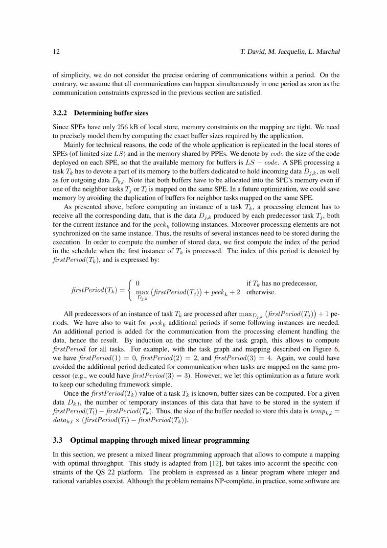
As presented above, before computing an instance of a task Tk, a processing element has toreceive all the corresponding data, that is the data Dj,k produced by each predecessor task Tj , bothfor the current instance and for the peekk following instances. Moreover processing elements are notsynchronized on the same instance. Thus, the results of several instances need to be stored during theexecution. In order to compute the number of stored data, we first compute the index of the periodin the schedule when the first instance of Tk is processed. The index of this period is denoted byfirstPeriod(Tk), and is expressed by:

firstPeriod(Tk) =

{

0 if Tk has no predecessor,maxDj,k

(

firstPeriod(Tj))

+ peekk + 2 otherwise.

All predecessors of an instance of task Tk are processed after maxDj,k

(

firstPeriod(Tj))

+ 1 pe-riods. We have also to wait for peekk additional periods if some following instances are needed.An additional period is added for the communication from the processing element handling thedata, hence the result. By induction on the structure of the task graph, this allows to computefirstPeriod for all tasks. For example, with the task graph and mapping described on Figure 6,we have firstPeriod(1) = 0, firstPeriod(2) = 2, and firstPeriod(3) = 4. Again, we could haveavoided the additional period dedicated for communication when tasks are mapped on the same pro-cessor (e.g., we could have firstPeriod(3) = 3). However, we let this optimization as a future workto keep our scheduling framework simple.

Once the firstPeriod(Tk) value of a task Tk is known, buffer sizes can be computed. For a givendata Dk,l, the number of temporary instances of this data that have to be stored in the system iffirstPeriod(Tl)− firstPeriod(Tk). Thus, the size of the buffer needed to store this data is tempk,l =datak,l × (firstPeriod(Tl)− firstPeriod(Tk)).

3.3 Optimal mapping through mixed linear programming

In this section, we present a mixed linear programming approach that allows to compute a mappingwith optimal throughput. This study is adapted from [12], but takes into account the specific con-straints of the QS 22 platform. The problem is expressed as a linear program where integer andrational variables coexist. Although the problem remains NP-complete, in practice, some software are


able to solve such linear programs [9]. Indeed, thanks to the limited number of processing elementsin the QS 22, we are able to compute the optimal solution for task graphs of reasonable size (up to afew hundreds of tasks).

Our linear programming formulation makes use of both integer and rational variables. The integervariables are described below. They can only take values 0 or 1.• α’s variables which characterize where each task is processed: αk

i = 1 if and only if task Tk ismapped on processing element PE i.• β’s variables which characterize the mapping of data transfers: βk,l

i,j = 1 if and only if data Dk,l

is transferred from PE i to PE j (note that the same processing element may well handle bothtask if i = j).

Obviously, these variables are related. In particular, βk,li,j = αk

i × αlj , but this redundancy al-

lows us to express the problem as a set of linear constraints. The objective of the linear programis to minimize the duration T of a period, which corresponds to maximizing the throughput ρ =1/T . The constraints of the linear program are detailed below. Remember that processing elementsPE 0, . . . ,PEnP−1 are PPEs whereas PEnP

, . . . ,PEn are SPEs.• α and β are integers.

∀Dk,l, ∀PE i and PE j , αki ∈ {0, 1}, β

k,li,j ∈ {0, 1} (10)

• Each task is mapped on one and only one processing element.

∀Tk,∑n−1

i=0 αki = 1 (11)

• The processing element computing a task holds all necessary input data.

∀Dk,l, ∀j, 0 ≤ j ≤ n− 1,∑n−1

i=0 (βk,li,j ) ≥ αl

j (12)

• A processing element can send the output data of a task only if it processes the correspondingtask.

∀Dk,l, ∀i, 0 ≤ i ≤ n− 1,∑n−1

j=0 (βk,li,j ) ≤ αk

i (13)

• The computing time of each processing element (PPE or SPE) is no larger that T .

∀i, 0 ≤ i < nP ,∑

Tk(αk

iwPPE(Tk)) ≤ T (14)

∀i, nP ≤ i < n,∑

Tk(αk

iwSPE(Tk)) ≤ T (15)

• All temporary buffers allocated on the SPEs fit into their local stores.

∀i, nP ≤ i < n,∑

Tk

(

αki

(

∑

Dk,ltempk,l +

∑

Dl,ktempl,k

))

≤ LS − code (16)

• A SPE can perform at most 16 simultaneous incoming DMA calls, and at most eight simulta-neous DMA calls are issued by PPEs on each SPE.

∀j, nP ≤ j < n,∑

0≤i<n,i 6=j

∑

Dk,lβk,li,j ≤ 16 (17)

∀i, nP ≤ i < n,∑

0≤j<nP

∑

Dk,lβk,li,j ≤ 8 (18)

• The amount of data communicated among processing elements during one period can be de-duced from β.

∀PE i and PE j , δi,j =∑

Dk,l

βk,li,j datak,l (19)

Using this definition, Equations (1), (2), (3), (4), (5), (6), (7), (8), and (9) ensure that allcommunications are performed within period T .


The size of the linear program depends on the size of the task graphs: it counts n |VA|+n2 |EA|+1variables.

We denote ρopt = 1/Topt , where Topt is the value of T in any optimal solution of the linearprogram. This linear program computes a mapping of the application that reaches the maximumachievable throughput. By construction, α is a valid mapping, and all possible mappings can bedescribed as α and β variables, which obey the constraints of the linear program.

4 Low-complexity heuristics

For large task graphs, solving the linear program may not be possible, or may take a very long time.This is why we propose in this section heuristics with lower complexity to find a mapping of the taskgraph on the QS 22. As explained in Section 3.2.1, the schedule which takes into account prece-dence constraints, naturally derives from the mapping. We start with straightforward greedy mappingalgorithms, and then move to more involved strategies.

We recall a few useful notations for this section: wPPE(Tk) denotes the processing time of task Tk

on any PPE, while wSPE(Tk) is its processing time on a SPE. For data dependency Dk,l between tasksTk and Tl, we have computed tempk,l, the number of temporary data that must be stored in steadystate. Thus, we can compute the overall buffer capacity needed for a given task Tk, which correspondsto the buffers for all incoming and outgoing data: buffers[k] =

∑

j 6=k(tempj,k + tempk,j).

4.1 Communication-unaware load-balancing heuristic

The first heuristic is a greedy load-balancing strategy, which is only concerned by computation, anddoes not take communication into account. Usually, such algorithms offer reasonable solutions whilehaving a low complexity.

This strategy first consider SPEs, since they hold the major part of the processing power of theplatform. The tasks are sorted according to their affinity with SPEs, and the tasks with larger affinityare load-balanced among SPEs. Tasks that do not fit in the local store of SPEs are mapped on PPEs.After this first step, some PPE might be underutilized. In this case, we then move some tasks whichhave affinity with PPEs from SPEs to PPEs, until the load is globally balanced. This heuristic will bereferred to as GREEDY in the following, and is detailed in Algorithm 1.

4.2 Prerequisites for communication-aware heuristics

When considering complex task graphs, handling communications while mapping tasks onto proces-sors is a hard task. This is especially true on the QS 22, which has several heterogeneous commu-nication links, and even within each of its Cell processors. The previous heuristic ignore commu-nications for the sake of simplicity. However, being aware of communications while mapping tasksonto processing element is crucial for performance. We present here a common framework to handlecommunications in our heuristics.

4.2.1 Partitioning the Cell in clusters of processing elements

As presented above, the QS 22 is made of several heterogeneous processing elements. In order tohandle communications, we first simplify its architecture and aggregate these processing elementsinto coarse-grain groups sharing common characteristics.


Algorithm 1: GREEDY(GA)

foreach Tk do affinity(Tk)←wSPE(Tk)wPPE(Tk)

foreach SPE i doworkload [SPE i]← 0memload [SPE i]← 0

foreach PPE j doworkload [PPE j ]← 0

foreach Tk in non decreasing order of affinity doFind SPE i such that workload [SPE i] is minimal and memload [SPE i]+ buffers[k] ≤ LSif there is such a SPE i then

mapping [Tk]← SPE i /* Map Tk onto SPE i */

workload [SPE i]← workload [SPE i] + wSPE(Tk)memload [SPE i]← memload [SPE i] + buffers[k]

elseFind PPE j such that workload [PPE j ] is minimalmapping [Tk]← PPE j /* Map Tk onto PPE j */

workload [PPE j ]← workload [PPE j ] + wPPE(Tk)

while the maximum workload of PPEs is smaller than the maximum workload of SPEs doLet SPE i be the SPE with maximum workloadLet PPE j be the PPE with minimum workloadConsider the list of tasks mapped on SPE i, ordered by non-increasing order of affinityFind the first task Tk in this list such thatworkload [PPE j ] + wPPE(Tk) ≤ workload [SPE i] andworkload [SPE i]− wSPE(Tk)) ≤ workload [SPE i]if there is such a task Tk then

Move Tk from SPE i to PPE j :mapping [Tk]← PPE j

workload [PPE j ]← workload [PPE j ] + wPPE(Tk)workload [SPE i]← workload [SPE i]− wSPE(Tk)memload [SPE i]← memload [SPE i]− buffers[k]

elseget out of the while loop

return mapping


If we take a closer look on the QS 22, we can see that some of the communication links are likelyto become bottlenecks. This is the case for the link between the PPEs and their respective set ofSPEs, and for the link between both Cell chips. Based on this observation, the QS 22 can therefore bepartitioned into four sets of processing elements, as shown in Figure 7. The communications withineach set are supposed to be fast enough. Therefore, their optimization is not crucial for performance,and only the communications among the sets will be taken into account.

PPE 1

PPE 2 C2

C1

tcommC1→PPE 1

tcommC1→C2

tcommPPE 1→C1

tcommC2→C1

tcommC2→PPE 2

tcommPPE 2→C2

Figure 7: Partition of the processing elements within the Cell

In order to estimate the performance of any candidate mapping of a given task graph on thisplatform, it is necessary to evaluate both communication and computation times. We adopt a similarview as developed above for the design of the linear program. Given a mapping, we estimate the timetaken by all computations and communications, and we compute the period as the maximum of allprocessing times.

As far as computations are concerned, we estimate the computation time tcompP of each part P of

processing element as the maximal workload of any processing element within the set. The workloadof a processing element PE is given by

∑

Tk∈SwSPE(Tk) in case of SPE, and by

∑

Tk∈SwPPE(Tk)

in case of a PPE, where S is the set of tasks mapped on the processing element.For communications, we need to estimate the data transfer times on every links interconnecting

the sets of processing elements, as represented on Figure 7. For each unidirectional communicationlink between two parts P1 and P2, we define tcomm

P1→P2as the time required to transfer every data going

through that link. We adopt a linear cost model, as in the previous section. Hence, the communicationtime is equal to the amount of data divided by the bandwidth of the link. We rely on the previousbenchmarks for the bandwidths:• The links links between the two Cell chips have a bandwidth of 13 GB/s (C1 → C2) and

11.5 GB/s (C2 → C1), as highlighted in Equations (7) and (8);• The links from a PPE to the accompanying set of SPEs (PPE 1 → C1 and PPE 2 → C2),

which correspond to a read operation from the main memory, have a bandwidth of 25 GB/s (seeEquation (2)).

The routing in this simplified platform is straightforward: for instance, the data transiting betweenPPE 1 and PPE 2 must go through links PPE 1 → C1, C1 → C2 and finally C2 → PPE 2. Formally,when DP1→P2

denotes the amount of data transferred from part P1 to part P2, the communicationtime of link C1 → C2 is given by:

tcommC1→C2

=DC1→C2

+DPPE1→C2+DC1→PPE2

+DPPE1→PPE2

13


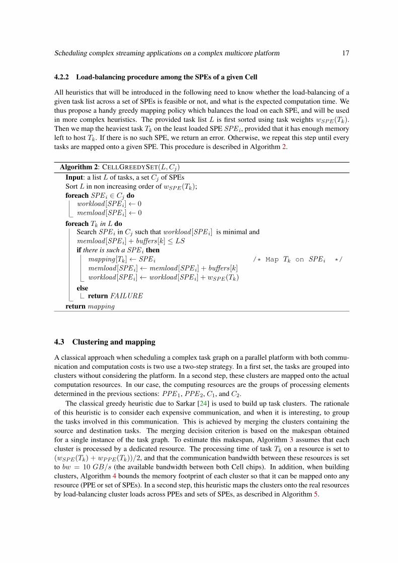
4.2.2 Load-balancing procedure among the SPEs of a given Cell

All heuristics that will be introduced in the following need to know whether the load-balancing of agiven task list across a set of SPEs is feasible or not, and what is the expected computation time. Wethus propose a handy greedy mapping policy which balances the load on each SPE, and will be usedin more complex heuristics. The provided task list L is first sorted using task weights wSPE(Tk).Then we map the heaviest task Tk on the least loaded SPE SPE i, provided that it has enough memoryleft to host Tk. If there is no such SPE, we return an error. Otherwise, we repeat this step until everytasks are mapped onto a given SPE. This procedure is described in Algorithm 2.

Algorithm 2: CELLGREEDYSET(L,Cj)

Input: a list L of tasks, a set Cj of SPEsSort L in non increasing order of wSPE(Tk);foreach SPE i ∈ Cj do

workload [SPE i]← 0memload [SPE i]← 0

foreach Tk in L doSearch SPE i in Cj such that workload [SPE i] is minimal andmemload [SPE i] + buffers[k] ≤ LSif there is such a SPE i then

mapping [Tk]← SPE i /* Map Tk on SPE i */

memload [SPE i]← memload [SPE i] + buffers[k]workload [SPE i]← workload [SPE i] + wSPE(Tk)

elsereturn FAILURE

return mapping

4.3 Clustering and mapping

A classical approach when scheduling a complex task graph on a parallel platform with both commu-nication and computation costs is two use a two-step strategy. In a first set, the tasks are grouped intoclusters without considering the platform. In a second step, these clusters are mapped onto the actualcomputation resources. In our case, the computing resources are the groups of processing elementsdetermined in the previous sections: PPE 1, PPE 2, C1, and C2.

The classical greedy heuristic due to Sarkar [24] is used to build up task clusters. The rationaleof this heuristic is to consider each expensive communication, and when it is interesting, to groupthe tasks involved in this communication. This is achieved by merging the clusters containing thesource and destination tasks. The merging decision criterion is based on the makespan obtainedfor a single instance of the task graph. To estimate this makespan, Algorithm 3 assumes that eachcluster is processed by a dedicated resource. The processing time of task Tk on a resource is set to(wSPE(Tk) + wPPE(Tk))/2, and that the communication bandwidth between these resources is setto bw = 10 GB/s (the available bandwidth between both Cell chips). In addition, when buildingclusters, Algorithm 4 bounds the memory footprint of each cluster so that it can be mapped onto anyresource (PPE or set of SPEs). In a second step, this heuristic maps the clusters onto the real resourcesby load-balancing cluster loads across PPEs and sets of SPEs, as described in Algorithm 5.


Algorithm 3: EPT (C): Estimated parallel time of the clustering C

foreach task Tk in reverse topological order do

maxoutlocal = max(

bl(Tm) such that (Tk, Tm) ∈ E and C(Tk) = C(Tm))

maxoutremote = max(

bl(Tm) +datak,m

bwsuch that (Tk, Tm) ∈ E and C(Tk) 6= C(Tm)

)

bl(Tk) =wPPE(Tk) + wSPE(Tk)

2+ max(maxoutlocal ,maxoutremote)

foreach task Tk in topological order do

maxinlocal = max(

tl(Tm) +wPPE(Tm) + wSPE(Tm)

2such that (Tm, Tk) ∈

E and C(Tm) = C(Tk))

maxinremote = max(

tl(Tm) +wPPE(Tm) + wSPE(Tm)

2+

datam,k

bwsuch that (Tm, Tk) ∈

E and C(Tm) 6= C(Tk))

tl(Tk) = max(maxinlocal ,maxinremote)

return max(bl(Tk) + tl(Tk))

Algorithm 4: CellClustering(GA)

In the initial clustering, each tasks of GA has its own cluster:foreach task Tk do Clustering(Tk) = kcompute EPT (Clustering)L← list of edges of the task graphSort L by non-increasing communication weightforeach edge (Tk, Tl) in L do

newClustering ← Clustering

Merge the clusters containing Tk and Tl:foreach task Ti do

if Clustering(Ti) = Clustering(Tl) thennewClustering(Ti)← Clustering(Tk)

compute EPT (newClustering)if EPT (newClustering) ≤ EPT (Clustering) and the CELLGREEDYSET greedy

heuristic successfully maps cluster newClustering(Tk) on a set of SPEs thenClustering ← newClustering


Algorithm 5: CellMapClusters(Clustering) : Map clusters into computing resourcesConsider a set of clusters Clustering built with Algorithm 4foreach cluster C in Clustering do

Compute the weight of cluster C: w(c) =∑

Tk∈C

wPPE(Tk) + wSPE(Tk)

Sort L by non-increasing weightsload(PPE 1)← 0, load(PPE 2)← 0foreach cluster C in Clustering do (we try to map C on each resource)

newload(PPE 1)← load(PPE 1) +∑

Tk∈CwPPE(Tk)

newload(PPE 2)← load(PPE 2) +∑

Tk∈CwPPE(Tk)

Run CELLGREEDYSET on C1 using the clusters already mapped to C1 plus C, computenewload(C1) as the maximum load of all SPEs in C1 (let newload(C1)←∞ ifCELLGREEDYSET fails)Do the same on C2 to compute newload(C2)Select the resource R such that newload(R) is minimumMap C on resource R: mapping [C]← Rif R is a PPE then load(R)← newload(R)

return mapping

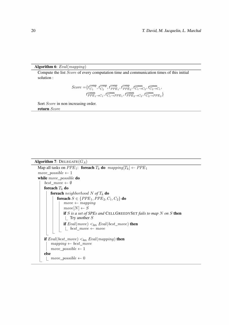
4.4 Iterative refinement using DELEGATE

In this Section, we present an iterative strategy to build an efficient allocation. This method, calledDELEGATE, is adapted from the heuristic introduced [12]. It consists in iteratively refining an al-location by moving some work from a highly loaded resource to a less loaded one, until the load isequally balanced on all resources. Here, resources can be either PPEs (PPE 1 or PPE 2) or set of SPEs(C1 or C2). In the beginning, all tasks are mapped on one of the PPE (PPE 1). Then, a (connected)subset of tasks is selected and its processing is delegated to another resource. The new mapping isselected if it respects memory constraints and improves the performance. This refinement procedureis then repeated until no more transfer is possible. If the selected resource for a move is a PPE, itis straightforward to compute the new processing time. If it is a set of SPEs, then the procedureCELLGREEDYSET is used to check memory constraints and compute the new processing time.

As in [12], at each step, a large number of moves are considered: for each task, all d-neighborhoodsof this task are generated (with d = 1, 2 . . . dmax), and mapped onto each available resource. Amongthis large set of moves, we select the one with best performance. This heuristic needs a more involvedway to compute the performance than simply using the period. Consider for example that both PPEsare equally loaded, but all SPEs are free. Then no move can directly decrease the period, but twomoves are needed to decrease the load of both PPEs. Thus, for a given mapping, we compute all con-tributions to the period: the load of each resource, and the time needed for communications betweenany pair of resources (the period is the maximum of all contributions). The list of these contributionsis sorted by non-increasing value. To compare two mappings, the one with the smallest contributionlist in lexicographical order is selected.


Algorithm 6: Eval(mapping)

Compute the list Score of every computation time and communication times of this initialsolution :

Score ={tcompC1

, tcompC2

, tcompPPE1

, tcompPPE2

, tcommC1→C2

, tcommC2→C1

,

tcommPPE1→C1

, tcommC1→PPE1

, tcommPPE2→C2

, tcommC2→PPE2

}

Sort Score in non increasing order.return Score

Algorithm 7: DELEGATE(GA)

Map all tasks on PPE 1: foreach Tk do mapping [Tk]← PPE 1

move_possible ← 1while move_possible do

best_move ← ∅foreach Tk do

foreach neighborhood N of Tk doforeach S ∈ {PPE 1,PPE 2, C1, C2} do

move ← mapping

move[N ]← Sif S is a set of SPEs and CELLGREEDYSET fails to map N on S then

Try another S

if Eval(move) <lex Eval(best_move) thenbest_move ← move

if Eval(best_move) <lex Eval(mapping) thenmapping ← best_move

move_possible ← 1else

move_possible ← 0


5 Experimental validation

This section presents the experiments conducted to validate the scheduling framework introducedabove. We first present the scheduling software developed to run steady-state schedules on the QS 22,then the application graphs in use, and finally report and comment the results.

5.1 Scheduling software

In order to run steady-state schedules on the QS 22, a complex software framework is needed: it hasto map tasks on different types of processing elements and to handle all communications. Althoughthere already exists some frameworks dedicated to streaming applications [15, 16], none of them isable to deal with complex task graphs while allowing to statically select the mapping. Thus, we havedecided to develop our own framework1. Our scheduler requires the description of the task graph,its mapping on the platform, and the code of each task. Even if it was designed to use the mappingreturned by the linear program, it can also use any other mapping, such as the ones dictated by thepreviously described heuristic strategies.

For now, our scheduling framework is able to handle only one PPE. For the following, we thusconsider nP = 1 PPE and nP = 16 SPE.

Once all tasks are mapped onto the right processing elements and the process is properly initial-ized, the scheduling procedure is divided into two main phases: the computation phase, when thescheduler selects a task and processes it, and the communication phase, when the scheduler performsasynchronous communications. These steps, depicted on Figure 8, are executed by every processingelements. Moreover, since communications have to be overlapped with computations, our schedulercyclically alternates between those two phases.

Select a Task

Wait for Resources

Process Task

Signal new Data

Communicate

Com

puta

tion

Pha

se

Communicate

(a) Computation Phase.

No more comm.

No

No

Com

mun

icat

ion

Pha

se

Compute

For each inbound comm.

Check input data

Watch DMA

Check input buffers

Get Data

(b) Communication Phase.

Figure 8: Scheduler state machine.

The computation phase, which is shown on Figure 8(a), begins with the selection of a runnable taskaccording to the provided schedule, and waits for the required resources (input data and output buffers)to be available. If all required resources are available, the selected task is processed, otherwise, itmoves to the communication phase. Whenever a new data is produced, the scheduler signals it to everydependent processing elements. Note that in our framework, computation tasks are not implemented

1An experimental version of our scheduling framework is available online, at http://graal.ens-lyon.fr/~mjacquel/cell_ss.html

http://graal.ens-lyon.fr/~mjacquel/cell_ss.html

http://graal.ens-lyon.fr/~mjacquel/cell_ss.html


as OS tasks but rather as function calls. One computing thread is launched on each processing element(PPE or SPEs). Each thread then internally chooses the next function (or node of the task graph) torun according to the provided schedule. This allows us to avoid fine task scheduling at the OS level.

The communication phase, depicted in Figure 8(b), aims at performing every incoming commu-nication, most often by issuing DMA calls. Therefore, the scheduler starts watching every previouslyissued DMA calls in order to unlock the output buffer of the sender as soon as data had been received.Then, the scheduler checks whether there is new incoming data. In that case, and if enough inputbuffers are available, it issues the proper “Get” command.

Libnuma [21] is used for both thread and memory affinity. Since a PPE can simultaneously handletwo threads, the affinity of every management threads is set to the first multi-threading unit, while PPEcomputing thread’s affinity is set to the second multi-threading unit. Therefore, management threadsand computing thread runs on different multi-threading units, and do not interfere. Moreover, the dataused by a given thread running on a PPE is always allocated on the memory bank associated to thatPPE.

To obtain a valid and efficient implementation of this scheduler, we had to overcome severalissues due to the very particular nature of the Cell processor. First, the main issue is heterogeneity:the Cell processor is made of two different types of cores, which induces additional challenges for theprogrammer:• SPE are 32-bit processors whereas the PPE is a 64-bit architecture;• Different communication mechanisms have to be used depending on which types of processing

elements are implied in the communication. To properly issue our “Get” operations, we madeuse of three different intrinsics: mfc_get for SPE to SPE communications, spe_mfcio_putfor SPE to PPE communication, and memcpy for communication between PPE and main mem-ory.

Another difficulty lies in the large number of variables that we need to statically initialize in each localstore before starting the processing of the stream: the information on the mapping, the buffer for datatransfer, and some control variables such as addresses of all memory blocks used for communications.This initialization phase is again complicated by the different data sizes between 32-bit and 64-bitarchitectures, and the run-time memory allocation.

All these issues show that the Cell processor is not designed for such a complex and decentralizedusage. However, our success in designing a complex scheduling framework proves that it is possibleto use such a heterogeneous processor for something else than pure data-parallelism.

5.2 Application scenarios

We test our scheduling framework on 25 random task graphs, obtained with the DagGen genera-tor [26]. This allows us to test our strategy against task graphs with different depths, widths, andbranching factors.

The smallest graph has 20 tasks while the largest has 135 tasks. The smallest graph is a simplechain of tasks, and the largest graph is depicted on Figure 9(a). On the communication side, thenumber of edges goes from 19 to 204, the graph with 204 edges is depicted on Figure 9(b).

We classified the generated graphs into two sets, one for the smaller graphs, having up to 59 tasks,and one for the larger graphs (87 - 135 tasks).

For all graphs, we generated 10 variants with different Communication-to-Computation Ratio(CCR), resulting in 250 different random applications and 230 hours of computation. We definethe CCR of a scenario as the total number of transferred elements divided by the total number of


operations on these elements. In the experiments, the CCR ranges from 0.001 (computation-intensivescenario) to 0.1 (communication-intensive scenario).

1

2

3

4

5

135

6 7

8

9

10 11 12 13 14 15 16

17

18

19

20

21

22 23 24 25

26

27 28 29

30

31

32

33

34

36

35 37 38 39 40

41

42

43

44

45

46

47

48 49

50

51

52

53

54

55

56

57

58 59 60 61

62

63

64 65

66

67

68

69 70

71

73

72

75

74

76

77

78

79

80

81 82

83

84

85

86

87 88 89 90 91

92

93

94

95 96

97

9899

100

101

102

103

105

104

106 107

108

109

110

111

114

112

113

115

116

117

118

119

120

121 122

123

124

125

126

127

128

129

130

131

132 133 134

(a) Graph with largest number of tasks

1

2

3 4

133

5

6

7 9

8

10

11

1415 16

12 1318 21

17

19

20

22 23

27

2534 28

2429 30

31

26 32

333538 37 36

45

47

414640

43 44

3942 48

5150 49

54 57586053

56

59

52

55

6265 6366 67 6461

72

68

75

77

70 69

7178

73

79 7476

80 8487

90

81

8689

838891 85

82

93 94

92 95

98

102 103104

100 97 99

96 101105

107

109 108 106

111

112115

116

113 114

110

118

123119 121 125 120 122124 127 128126 130

117129

132131

(b) Graph with largest number of edges

Figure 9: Largest task graphs used in the experiments

In the experiments, we denote by MIP the scheduling strategy using Mixed Integer Programmingto compute an optimal mapping, and described in Section 3.3. ILOG CPLEX [9] is used to solve thelinear program with rational and integer variables. To reduce the computation time for solving thelinear program, we used the ability of CPLEX to stop its computation as soon as its solution is within5% of the optimal solution. While this significantly reduces the average resolution time, it still offersa very good solution.

5.3 Experimental results

In this section, we present the performance obtained by the scheduling framework presented above.We first focus on the initialization phase of streaming applications using our framework, showingthat steady-state operation is reached within a reasonable amount of instances. Then, we comparethe throughput obtained by the heuristics introduced in Section 4 and the algorithm MIP, both usingthe model of the QS 22 and using experiments on a real platform. Finally, we discuss the impact ofthe communication-to-computation ration, and estimate the time required to compute mappings usingeach strategy. Note that except when we study the influence of the number of SPEs, all the resultspresented below are computed using all 16 SPEs in the QS 22.

5.3.1 Entering steady-state

First, we show that our scheduling framework succeeds in reaching steady-state, and that the through-put is then similar to the one predicted by the linear program. Figure 10 shows the experiments donewith the task graph described in Figure 9(b), with a CCR of 0.004, on the QS 22 using all 16 SPEs.

We notice that a steady-state operation is obtained after processing approximately 1000 instances.Note that the input data of one instance consists only of a few bytes, so the duration of the tran-sient phase before reaching the steady-state throughput is small compared to the total duration of the


stream. In steady state, the experimental throughput achieves 95% of the theoretical throughput pre-dicted by the linear program. The small gap is explained by the overhead of our framework, and thesynchronizations induced when communications are performed. The schedules given by other map-pings, computed using heuristics, also reaches steady state after a comparable transient phase. Wediscuss their steady-state throughput below.

Thr

ough

put(

inst

ance

/sec

)

1500 1750 2000 2250

Number of instances

0

1

2

3

4

5

6

7

8

9

10

11

12

0 250 500 750 1000 1250

GREEDY

Experimental MIPDELEGATE

Using a single PPECLUSTER

Theoretical MIP

Figure 10: Throughput achieved depending on the number of instances.

In Table 1, we present the number of instances that are required to reach steady state, that is, toreach 99% of the maximum (experimental) throughput, for all possible scenarios. The average valueis around 2000 instances, but the mapping computed using MIP reaches steady state faster than theother solutions. We have observed the same behavior on small and large task graphs. This shows thatour scheduling framework is able to reach steady-state operation for any mapping within a reasonableamount of instances compared to the usual length of streaming applications.

Algorithm Min. Max. Average Std. dev.GREEDY 300 18,500 2,234 2,589

DELEGATE 250 16,500 2,249 2,381CLUSTER 300 14,600 2,214 2,586

MIP 300 14,500 2,050 2,182

Table 1: Number of instances required to reach steady state for all scenarios.

Figure 11(a) presents the distribution of the ratio between the experimental throughput of MIP,and the theoretical throughput (the one predicted by the linear program). The average ratio is 0.91,but we can observe that the experimental throughput is sometimes very different from the theoreticalone (as less as 20% or as much as 597%). Cases when the experimental throughput is 5 times smallerthan the predicted one mainly happen for small task graphs, when the very few tasks are scheduledon each processing elements, which leads to a high synchronization cost. Figure 11(b) shows theresults for large task graphs, when the accuracy of the predicted throughput is larger (the average


ratio is 1.10). There still remain some cases with a high ratio (the experimental throughput is largerthan the predicted throughput). This corresponds to communication-intensive scenarios: in a fewcases, our communication model is very pessimistic for communications and overestimates bandwidthcontention.

1 2 3 4 5 6

Experimental/theoretical mip throughput

0

5

10

15

20

25

30

Freq

uenc

y(%

)

(a) All task graphs

1 1.5 2 2.5 3 3.5 4

Experimental/theoretical mip throughput

0

10

20

30

40

50

60

Freq

uenc

y(%

)

(b) Large task graphs

Figure 11: Distribution of the ratio between experimental and theoretical throughputs for the MIPstrategy.

5.3.2 Theoretical comparison of heuristics with MIP

We first start by comparing the expected throughput of the heuristics described in Section 4 withthe theoretical throughput of MIP, detailed in Section 3.3. This allows to measure the quality ofthe mapping produced by heuristics without the particularities of the scheduling framework, and theinaccuracies of the QS 22 model.

For this purpose, we first compute the theoretical throughput of all mappings produced by theheuristics. A mapping is first described using the α and β variables from the linear program presentedin Section 3.3. The expected period of the mapping can then be computed using Constraints (14)and (15) (for computations) and Constraints (1), (2), (3), (4), (5), (6), (7), (8), and (9) (for communi-cations).

This theoretical comparison also helps to assess the limitation of the constraints on DMA calls.In the design of the MIP strategy, the limited number of simultaneous DMA calls for PPEs andSPEs is taken into account with two Constraints (Equations (17) and (18)). This limitation is nottaken into account while designing heuristics, because we want to keep their design simple. Ourscheduling framework assigns DMA calls dynamically to communication requests, and is able to dealwith any number of communications. Of course, when the number of simultaneous communicationsexceeds the bounds, communications are delayed, thus impacting the throughput. The comparison oftheoretical throughput of mappings allows us to measure the limitation on the expected throughputinduced by these constraints, which only exist for MIP.

We hence compute the ratio between predicted throughput of heuristic strategies over the predictedthroughput of MIP. Detailed results are given in Table 2.

These results show that in some cases, the limitation on the number of DMA calls has an impacton the throughput: there are cases when the CLUSTER strategy finds a mapping with an expectedthroughput twice the one of MIP. The MIP strategy is able to reach the best throughput among allstrategies in only 80% of the scenarios, due to this limitation. However, MIP still gives a betteraverage throughput than all other strategies. Thus, this limitation has a little impact on performance.


All task graphsAlgorithm Min. Max. Average Std. dev. Best cases

GREEDY 0.55 1.49 0.82 0.12 6%DELEGATE 0.75 1.05 0.97 0.07 60%CLUSTER 0.00 2.46 0.32 0.28 1%

MIP 1.00 1.00 1.00 0.00 80%

Small task graphsAlgorithm Min. Max. Average Std. dev. Best cases


MIP 1.00 1.00 1.00 0.00 78%

Large task graphsAlgorithm Min. Max. Average Std. dev. Best cases


MIP 1.00 1.00 1.00 0.00 88%

Table 2: Predicted throughput of heuristics normalized to the predicted throughput of MIP

Among heuristics, the DELEGATE strategy ranks first: it is almost within 25% of the performanceof MIP, and on average gives the same results, and gives the best performance on 60% of the scenar-ios. (Note that several heuristics may give the best throughput for a scenario, hence leading to a sumlarger than 100%). Quite surprisingly, the CLUSTER strategy gives very poor results: on average itsthroughput is only one third of the MIP throughput, whereas the simple GREEDY strategy performsbetter, with an average throughput around 80% of the MIP throughput. All heuristics perform betteron small task graphs, and have more difficulties to tackle the higher complexity of large task graphs.

The bad performance of CLUSTER is surprising because this heuristics takes communication intoaccount, as opposed to GREEDY. However, the communications are considered only when buildingclusters in the first phase. In the second phase, when clusters are mapped on the resources, communi-cations are totally neglected. However, all communications do not have the same impact, because thecommunication graph has heterogeneous links. Moreover, since clusters have been made to cancelout the impact of large communications, the load balancing procedure in the second phase has lessfreedom, and is unable to reach a well balanced mapping. This explains why the mapping producedby CLUSTER are usually worse than the one given by DELEGATE or GREEDY.

5.3.3 Experimental comparison of heuristics with MIP

We move to the experimental comparison of heuristics and MIP, when all mappings are scheduledwith our scheduling software on the real QS 22 platform. The experimental throughputs of generatedmappings are presented in Table 3. For sake of comparison, all throughputs are normalized by thethroughput of MIP.

The comparison between heuristics and MIP is close to the one with expected throughputs. How-


All task graphsAlgorithm Min. Max. Average Std. dev. Best cases


MIP 1.00 1.00 1.00 0.00 54%

Small task graphsAlgorithm Min. Max. Average Std. dev. Best cases


MIP 1.00 1.00 1.00 0.00 46%

Large task graphsAlgorithm Min. Max. Average Std. dev. Best cases


MIP 1.00 1.00 1.00 0.00 80%

Table 3: Experimental throughput of heuristics normalized to the experimental throughput of MIP

ever, the gap between MIP and each heuristic is smaller: heuristics perform somewhat better onthe real platform that on the model. The average throughput of DELEGATE is very close to MIP’sthroughput (larger for small task graphs, but smaller for large task graphs), and GREEDY gets around90% of the MIP’s throughput. Once again, CLUSTER gives a very limited average throughput, withonly 41% of the MIP’s throughput. On large task graphs, MIP is above all heuristics, and reaches thebest throughput in 80% of the cases. However, on average, DELEGATE is able to achieve 95% of theMIP’s throughput.

5.3.4 Scaling and influence of the communication-to-computation ratio

In this section, we present the speed-up obtained by MIP and heuristics. We also study the influence ofthe Communication-to-Computation Ratio (CCR), both on the duration of the transient phase beforereaching steady state, and on the accuracy of the model.

We first present the performance obtained by all strategies, with different number of SPEs. Inthe MIP solution, the number of SPEs is a parameter, which may vary between 0 and 16. For allheuristics developed above, it is quite straightforward to adapt them to deal with a variable numberof SPEs. Figure 12 present the average speed-up of each heuristic obtained for different number ofSPEs. We observe that all heuristics are able to take advantage of an increasing number of SPEs.When the CCR is high, the resulting speed-up is smaller than when the CCR is low, because largecommunications make it more difficult to distribute tasks among processing elements. This is alsooutlined by Figure 13(b), which presents the variation of the average speed-up of heuristics (for 16SPEs) with the CCR. For a CCR smaller than 0.02, the average speed-up is almost constant, while itdecreases for a larger CCR. We can observe that DELEGATE is a little less sensitive to the increase


0 2 4 6 8 10 12 14 16

Number of SPE used

0

1

2

3

4

5

6

Ave

rage

spee

dup

GREEDY


CLUSTER

(a) With CCR=0.001

0 2 4 6 8 10 12 14 16

Number of SPE used

0

1

2

3

4

5

6

Ave

rage

spee

dup

GREEDY


CLUSTER

(b) With CCR=0.1

Figure 12: Average speed-up vs. number of SPEs in use.

of the CCR than MIP. For some strategies, the speed-up slightly increases when the CCR increasesfrom 0.001 to 0.02. This is because to increase the CCR, we first decrease the computation amount oftasks, which makes the overhead of the scheduling software more visible when all tasks are scheduledon the PPE.

All task graphs, CCR of 0.001Algorithm Min. Max. Average Std. dev.

GREEDY 300 400 367 38DELEGATE 300 400 367 42CLUSTER 300 400 361 40

MIP 300 400 375 35

All task graphs, CCR of 0.1Algorithm Min. Max. Average Std. dev.

GREEDY 200 4750 788 974DELEGATE 200 4200 750 850CLUSTER 150 2950 702 681

MIP 150 3200 646 670

Table 4: Number of instances required to reach steady state

Table 4 presents the number of instances that are processed in the transient phase before reachingsteady state, for the two extreme values of CCR: 0.001 (computation-intensive scenario) and 0.1(communication-intensive scenario). We observe that the larger the CCR, the longer the duration ofthe transient phase: when communications are predominant, it is more difficult to reach a steady statephase even if communications are well overlapped by computations.

Figure 13(a) presents the evolution of the ratio between the experimental throughput of MIP overits predicted throughput in function of the CCR. We notice that for all CCR smaller than 0.05, ourmodel is slightly optimistic, and predicts a throughput at most 30% larger than the one obtained inthe experiments. For larger CCRs, corresponding to communication-intensive scenarios, the model ispessimistic and larger throughputs are obtained in the experiments. Our model is thus best suited foraverage values of the CCR. In case of extreme values, it is necessary to modify the model, either bytaking into account synchronization costs, when CCR is very small, or by better modeling contentionbetween communications, in case of a very large CCR.

5.3.5 Time required to compute schedules

When considering streaming application, it is usually assumed that streams have very long durations.This is why it is worth spending some time to optimize the schedule before the real data process-ing. Yet, since we are using mixed linear programming, we report the time needed to compute the


0.001 0.01 0.1

CCR

0

0.2

0.4

0.6

0.8

1

1.2

1.4

1.6

Exp

erim

enta

l/Pre

dict

edM

IPT

hrou

ghpu

t

(a) Model accuracy vs. CCR

0.001 0.01 0.1

CCR

0

2

4

6

8

10

Ave

rage

spee

dup

GREEDY


CLUSTER

(b) Average speed-up vs. CCR

Figure 13: Evolution of the model accuracy and the speedup with the CCR.

schedules, to prove that this is done in reasonable time.Table 5 presents the time required to compute mappings using each algorithm. On average, the

MIP strategy requires twice as much time than all heuristics, and runs for less than two minutes.In some cases, corresponding to large graphs, the run time of MIP can reach 12 minutes, whereasDELEGATE need at most 3 minutes. These running, although large, are very reasonable in the contextof streaming applications that are supposed to run for several minutes or hours.

Algorithm Min. Max. Average

GREEDY 2.7 189 39CLUSTER 2.6 190 39

DELEGATE 2.9 205 48MIP 3.6 706 80

Table 5: Scheduling time in seconds

6 Related Work

Scheduling streaming applications is the subject of a vast literature. Several models and frameworkshad been introduced like StreamIt [25], Brook [10] or Data Cutter Lite [7]. However, our motivationfor this work was rather to extract a simple and yet relevant model for the Cell processor, so as tobe able to provide a way to compute interesting mapping for pipeline applications. To the best ofour knowledge, this has never been considered for the Cell processor, nor for another multi-corearchitecture that exhibits a similar heterogeneity. Note that the small scale of the target architecturemakes the problem very particular, and that it was not clear that such complex mapping techniquescould result in a feasible and competitive solution for streaming applications. To the best of ourknowledge, none of the existing frameworks which target the Cell processor make it is possible toimplement our own static scheduling strategies. The main two limitations of existing frameworks arethe restriction to simple pipeline applications (chain task graphs), whereas we target any DAG, andthe fact that only SPEs are used for computation, the PPE being restricted to control, whereas we takeadvantage of the heterogeneity.


Hiding memory accesses latencies is a crucial need when considering the Cell processor. In [14],the authors introduce an improvement to the Decoupled Threaded Architecture [13] consisting in aprefetching mechanism. They propose an implementation of this mechanism on the Cell processorthrough the use of DMA calls and extensions to compiler instructions set, which interest is demon-strated through simulation (no real implementation seems to be available). In our scheduler, we pro-pose a real implementation of a similar prefetching mechanism.

7 Conclusion

In this paper, we have studied the scheduling of streaming applications on a heterogeneous platform:the IBM Bladecenter QS 22, made of two heterogeneous multi-core Cell processors. The first chal-lenge was to come up with a realistic and yet tractable model of the Cell processor. We have designedsuch a model, and we have used it to express the optimization problem of finding a mapping with max-imal throughput. This problem has been proven NP-complete, and we have designed a formulation ofthe problem as a mixed linear program. By solving this linear program with appropriate tools, we cancompute a mapping with optimal throughput. We have also proposed a set of scheduling heuristics toavoid the complexity of mixed linear programing.

In a second step, we have implemented a complete scheduling framework to deploy streamingapplications on the QS 22. This framework, available for public use, allows the user to deploy anystreaming application, described by a potentially complex task graph, on a QS 22 platform or singleCell processor, given any mapping of the application to the platform. Thanks to this schedulingframework, we have been able to perform a comprehensive experimental study of all our schedulingstrategies. We have shown that our MIP strategy usually reaches 90% of the throughput predicted bythe linear program, that it has a good and scalable speed-up when using up to 16 SPEs. Some of theproposed heuristics, in particular DELEGATE, are also able to reach very good performance. Whenthe task graph to schedule is large, MIP is the one which offers the best performance, but DELEGATE

achieves 95% of its throughput on average. We have shown that considering load-balancing amongprocessing elements, and carefully estimating communications between the different components ofthis bi-Cell platform, is the key to performance.

Overall, this demonstrates that scheduling a complex application on a heterogeneous multi-coreprocessor is a challenging task, but that scheduling tools can help to achieve good performance.

This work has several natural extensions, which includes refining the model presented for theQS 22 to more complex platform, for example to consider a cluster of QS 22, or other multi-coreplatform.

References

[1] M. Ålind, M. Eriksson, and C. Kessler. BlockLib: a skeleton library for Cell broadband engine.In IWMSE ’08: Proceedings of the 1st international workshop on Multicore software engineer-

ing, pages 7–14. ACM, 2008.

[2] AMD Fusion. http://fusion.amd.com.

[3] Kevin J. Barker, Kei Davis, Adolfy Hoisie, Darren J. Kerbyson, Mike Lang, Scott Pakin, andJose C. Sancho. Entering the petaflop era: the architecture and performance of roadrunner. InSC ’08: Proceedings of the 2008 ACM/IEEE conference on Supercomputing, pages 1–11, 2008.

http://fusion.amd.com


[4] O. Beaumont, A. Legrand, L. Marchal, and Y. Robert. Steady-state scheduling on heterogeneousclusters. International Journal of Foundations of Computer Science, 16(2):163–194, 2005.

[5] Olivier Beaumont and Loris Marchal. Steady-state scheduling. In Introduction to Scheduling,pages 159–186. Chapman and Hall/CRC Press, 2010.

[6] Pieter Bellens, Josep M. Pérez, Felipe Cabarcas, Alex Ramírez, Rosa M. Badia, and JesúsLabarta. CellSs: Scheduling techniques to better exploit memory hierarchy. Scientific Pro-

gramming, 17(1-2):77–95, 2009.

[7] Michael D. Beynon, Tahsin M. Kurç, Ümit V. Çatalyürek, Chialin Chang, Alan Sussman, andJoel H. Saltz. Distributed processing of very large datasets with datacutter. Parallel Computing,27(11):1457–1478, 2001.

[8] ClearSpeed technology. http://www.clearspeed.com/technology/index.php.

[9] ILOG CPLEX: High-performance software for mathematical programming and optimization.http://www.ilog.com/products/cplex/.

[10] William J. Dally, Francois Labonte, Abhishek Das, Patrick Hanrahan, Jung-Ho Ahn, JayanthGummaraju, Mattan Erez, Nuwan Jayasena, Ian Buck, Timothy J. Knight, and Ujval J. Kapasi.Merrimac: Supercomputing with streams. In SC ’03: Proceedings of the 2003 ACM/IEEE

conference on Supercomputing, page 35, Washington, DC, USA, 2003. IEEE Computer Society.

[11] Kayvon Fatahalian, Daniel Reiter Horn, Timothy J. Knight, Larkhoon Leem, Mike Houston,Ji Young Park, Mattan Erez, Manman Ren, Alex Aiken, William J. Dally, and Pat Hanra-han. Memory - sequoia: programming the memory hierarchy. In SC ’06: Proceedings of the

ACM/IEEE conference on Supercomputing, page 83, 2006.

[12] Matthieu Gallet, Loris Marchal, and Frédéric Vivien. Efficient scheduling of task graph collec-tions on heterogeneous resources. In IEEE International Parallel and Distributed Processing

Symposium, 2009.

[13] Roberto Giorgi, Zdravko Popovic, and Nikola Puzovic. Dta-c: A decoupled multi-threadedarchitecture for cmp systems. In SBAC-PAD, pages 263–270, 2007.

[14] Roberto Giorgi, Zdravko Popovic, and Nikola Puzovic. Exploiting DMA to enable non-blockingexecution in decoupled threaded architecture. In IEEE International Parallel and Distributed

Processing Symposium, 2009.

[15] X. Hang. A streaming computation framework for the Cell processor. Master’s thesis, Mas-sachusetts Institute of Technology, 2007.

[16] T. Hartley and U. Catalyurek. A component-based framework for the Cell broadband engine. InIEEE International Parallel and Distributed Processing Symposium, 2009.

[17] Stephen L. Hary and Fusun Ozguner. Precedence-constrained task allocation onto point-to-pointnetworks for pipelined execution. IEEE Trans. Parallel and Distributed Systems, 10(8):838–851,1999.

[18] Ibm software kit for multicore acceleration. http://www.ibm.com/chips/techlib/

techlib.nsf/products/IBM_SDK_for_Multicore_Acceleration.

http://www.clearspeed.com/technology/index.php

http://www.ilog.com/products/cplex/

http://www.ibm.com/chips/techlib/techlib.nsf/products/IBM_SDK_for_Multicore_Acceleration

http://www.ibm.com/chips/techlib/techlib.nsf/products/IBM_SDK_for_Multicore_Acceleration


[19] James A. Kahle, Michael N. Day, H. Peter Hofstee, Charles R. Johns, Theodore R. Maeurer,and David J. Shippy. Introduction to the cell multiprocessor. IBM Journal of Research and

Development, 49(4-5):589–604, 2005.

[20] Michael Kistler, Michael Perrone, and Fabrizio Petrini. Cell multiprocessor communicationnetwork: Built for speed. IEEE Micro, 26(3):10–23, 2006.

[21] Andreas Kleen. A numa api for linux. http://andikleen.de/, 2005.

[22] Mercury technology. http://www.mc.com/technologies/technology.aspx.

[23] Ibm bladecenter qs22. http://www-03.ibm.com/systems/bladecenter/

hardware/servers/qs22/.

[24] Vivek Sarkar. Partitioning and Scheduling Parallel Programs for Multiprocessors. MIT Press,Cambridge, MA, USA, 1989.

[25] Streamit project. http://groups.csail.mit.edu/cag/streamit/index.

shtml.

[26] F. Suter. DAG generation program. http://www.loria.fr/~suter/dags.html.

[27] William Thies. Language and Compiler Support for Stream Programs. PhD thesis, Mas-sachusetts Institute of Technology, 2001.

[28] Q. Wu, J. Gao, M. Zhu, N.S.V. Rao, J. Huang, and S.S. Iyengar. On optimal resource utilizationfor distributed remote visualization. IEEE Trans. Computers, 57(1):55–68, 2008.

A Complete benchmark results

The following tables presents the measuder bandwidth and latency when performing a “read” opera-tion from a SPE to a distant local store. Table 6 presents the average latency for such a transfer, whileTable 7 shows the obtained bandwidth for a large transfer.

http://andikleen.de/

http://www.mc.com/technologies/technology.aspx

http://www-03.ibm.com/systems/bladecenter/hardware/servers/qs22/

http://www-03.ibm.com/systems/bladecenter/hardware/servers/qs22/

http://groups.csail.mit.edu/cag/streamit/index.shtml

http://groups.csail.mit.edu/cag/streamit/index.shtml

http://www.loria.fr/~suter/dags.html


Reader Distant local storeSPE 0 1 2 3 4 5 6 7 8 9 10 11 12 13 14 15

0 120 128 120 128 113 128 113 113 428 443 443 450 450 443 443 4501 113 128 113 120 113 143 113 128 458 420 450 443 450 413 465 4652 113 113 128 120 128 120 113 113 450 443 428 420 443 435 443 4503 120 113 128 120 120 128 113 128 450 458 450 443 435 435 428 4354 120 135 128 113 113 113 113 128 465 458 458 435 443 443 443 4435 113 113 113 113 113 113 113 120 450 450 443 435 450 450 458 4506 113 113 113 113 113 120 113 113 458 435 443 435 405 443 450 4507 113 113 128 113 113 113 113 120 435 450 450 450 435 458 450 4508 480 458 488 473 473 473 458 443 113 113 113 113 113 113 113 1139 450 480 473 495 428 458 480 458 113 113 113 113 113 113 113 11310 443 443 428 465 443 450 443 443 113 113 113 113 113 113 113 11311 480 473 458 488 465 473 443 465 113 120 113 113 113 113 113 11312 458 450 450 458 458 465 443 435 113 113 113 113 113 113 113 12813 458 420 435 450 480 443 443 450 113 113 120 113 113 113 113 11314 443 443 428 450 458 443 435 450 128 113 120 113 113 113 113 11315 450 488 435 435 443 450 458 435 113 113 113 113 113 113 113 113

Table 6: Latency when a SPE reads from a distant local store, in nanoseconds.

Reader Distant local storeSPE 0 1 2 3 4 5 6 7 8 9 10 11 12 13 14 15

0 23.1 23.4 24.2 24.8 24.8 23.9 23.5 23.9 4.9 4.8 4.9 4.9 4.9 5.1 4.9 5.11 23.9 23.7 23.4 24.5 23.2 24.5 23.6 24.2 4.9 4.9 4.8 4.9 5.0 4.8 4.9 4.82 23.9 24.2 23.1 24.2 23.0 23.4 23.7 23.9 5.0 4.9 4.9 4.8 5.0 4.9 5.0 4.93 24.5 23.9 24.2 23.5 22.3 24.0 25.1 24.8 5.1 4.7 4.9 5.0 4.9 4.9 4.9 5.04 25.4 25.4 23.9 25.1 25.4 25.4 25.4 25.4 4.9 5.0 5.0 5.0 5.0 5.0 4.8 4.85 25.4 25.4 24.0 25.4 25.4 25.4 24.8 25.4 4.9 4.8 4.8 4.8 5.0 4.9 4.9 4.96 25.1 25.1 25.1 25.4 24.8 25.4 25.4 24.8 4.9 4.9 4.9 4.9 4.9 5.0 5.0 5.07 24.3 25.1 24.5 25.1 23.1 24.6 25.1 24.5 4.9 5.0 4.8 4.8 4.9 4.8 4.9 5.18 3.3 3.3 3.5 3.4 3.4 3.4 3.5 3.5 25.4 25.4 24.8 25.1 25.4 25.4 25.4 25.49 3.5 3.3 3.5 3.3 3.3 3.4 3.5 3.5 25.4 25.4 24.8 25.1 24.5 25.1 25.4 25.410 3.3 3.3 3.4 3.4 3.4 3.4 3.5 3.3 25.4 25.4 24.6 25.1 24.8 25.4 25.4 25.111 3.5 3.3 3.4 3.3 3.4 3.4 3.3 3.4 25.4 25.4 25.1 25.4 25.4 25.4 25.4 25.412 3.3 3.3 3.4 3.3 3.5 3.4 3.4 3.4 25.4 25.4 25.4 25.1 25.4 25.4 24.6 25.413 3.3 3.2 3.4 3.3 3.3 3.3 3.3 3.4 25.4 25.4 25.1 24.8 25.4 25.4 25.4 25.414 3.4 3.3 3.4 3.4 3.4 3.3 3.5 3.5 25.4 25.1 24.8 25.4 25.4 25.4 25.4 25.415 3.4 3.4 3.5 3.4 3.4 3.3 3.4 3.4 25.1 25.4 24.3 25.4 25.4 25.1 25.1 25.4

Table 7: Bandwidth when a SPE reads from a distant local store, in GB/s.

scheduling streaming applications on a complex multicore

Documents