schechter siggraph2012 ghostsph

ACM Reference FormatSchechter, H., Bridson, R. 2012. Ghost SPH for Animating Water. ACM Trans. Graph. 31 4, Article 61 (July 2012), 8 pages. DOI = 10.1145/2185520.2185557 http://doi.acm.org/10.1145/2185520.2185557.

Copyright NoticePermission to make digital or hard copies of part or all of this work for personal or classroom use is granted without fee provided that copies are not made or distributed for profi t or direct commercial advantage and that copies show this notice on the fi rst page or initial screen of a display along with the full citation. Copyrights for components of this work owned by others than ACM must be honored. Abstracting with credit is permitted. To copy otherwise, to republish, to post on servers, to redistribute to lists, or to use any component of this work in other works requires prior specifi c permission and/or a fee. Permissions may be requested from Publications Dept., ACM, Inc., 2 Penn Plaza, Suite 701, New York, NY 10121-0701, fax +1 (212) 869-0481, or [email protected].© 2012 ACM 0730-0301/2012/08-ART61 $15.00 DOI 10.1145/2185520.2185557 http://doi.acm.org/10.1145/2185520.2185557

Ghost SPH for Animating Water

Hagit Schechter∗

University of British Columbia

Robert Bridson∗

University of British Columbia

Abstract

We propose a new ghost fluid approach for free surface and solidboundary conditions in Smoothed Particle Hydrodynamics (SPH)liquid simulations. Prior methods either suffer from a spurious nu-merical surface tension artifact or drift away from the mass con-servation constraint, and do not capture realistic cohesion of liquidto solids. Our Ghost SPH scheme resolves this with a new particlesampling algorithm to create a narrow layer of ghost particles in thesurrounding air and solid, with careful extrapolation and treatmentof fluid variables to reflect the boundary conditions. We also pro-vide a new, simpler form of artificial viscosity based on XSPH. Ex-amples demonstrate how the new approach captures real liquid be-haviour previously unattainable by SPH with very little extra cost.

CR Categories: Computer Graphics [I.3.7]: Three-DimensionalGraphics and Realism—Animation; Computer Graphics [I.3.5]:Computational Geometry and Object Modeling—Physically basedmodeling

Keywords: Smoothed Particles Hydrodynamics, SPH, free sur-face, boundary conditions, volume sampling, liquids, animation

Links: DL PDF

1 Introduction

Animating liquids like water via physical simulation remains a be-guiling area. Many methods have been developed in graphics tosolve various problems, both for realism of the results and for per-formance. Our focus here is Smoothed Particle Hydrodynamics(SPH), where the fluid is represented by material particles withrelatively simple interactions via sums of smooth kernel functionsand their gradients: see Monaghan for a detailed overview [2005],which we assume as background knowledge. Most SPH methodsenjoy automatic mass conservation (each particle represents a fixedamount of conserved mass, density is estimated by direct sum-mation), accurate tracking of the fluid through space (due to theLagrangian representation), and a conceptually simple algorithmickernel (summing weighted kernels over nearby particles, with nosystems of equations to solve or tricky geometric discretizations).

However, several problems remain: here we tackle the treatment offree surface and solid boundary conditions. Mass-conserving SPHmethods, where density is estimated by a sum rather than evolved asa state variable, suffer serious errors near free surfaces causing un-avoidable surface-tension-like artifacts and reduced stability. Prior

∗e-mail: (hagitsch|rbridson)@cs.ubc.ca

Figure 1: With our new boundary conditions, water pouring on toa sphere properly coheres to the underside, giving a realistic streamwithout excessive numerical surface tension.

treatments of arbitrary solid boundaries do not reflect the correct co-hesive behaviour visible in many real world scenarios. Our GhostSPH method resolves both by careful sampling of ghost particlesin the air and solid regions near the fluid, and appropriate extrapo-lation of fluid quantities to the ghost particles. Our new samplingalgorithm, an extension of a Poisson-disk method which accuratelycaptures boundaries, is also of interest to other applications.

2 Related Work

SPH was independently introduced by Gingold and Monaghan[1977] and Lucy [1977], and has since seen extensive use in physicsresearch. The advantages above have also made it popular in com-puter graphics for a variety of liquid phenomena.

Monaghan’s adaptation [1994] of SPH to free-surface flow servesas a basis for many later works. Muller et al. [2003] useda low stiffness equation of state along with surface tension andviscosity forces for interactive applications. Refined particlesampling near free surfaces for accuracy or efficiency is dis-cussed in several works [Keiser et al. 2006; Adams et al. 2007;Solenthaler and Gross 2011]. Becker and Teschner [2007] reducecompressibility with the stiffer “Tait Equation”, and introduce par-ticle initialization with highly damped equations to reach a stabledensity near the surface, which we directly solve with ghost air par-ticles.

Muller et al. seeded air particles to model bubbles [2003]. Keiseralso used a narrow band of air particles to aid in surface tension andsmall bubbles [2006] — however, whereas this work’s mirroringapproach may create air sampling with widely varying density, wealways seed ghost air particles with a near-rest-state distribution.

Bonet and Kulasegaram [2002] modified the underlying SPH

ACM Transactions on Graphics, Vol. 31, No. 4, Article 61, Publication Date: July 2012

http://doi.acm.org/10.1145/2185520.2185557

http://portal.acm.org/ft_gateway.cfm?id=2185557&type=pdf

method with corrections to make the scheme numerically consis-tent, resolving density problems near boundaries as we do, but withsignificantly heavier calculation.

Muller et al [2005] achieved two-way SPH fluid interaction using“color field”-derived curvature. Solenthaler and Pajarola [2008]introduced a modified density equation for accurate SPH densitycomputation at the interface between the two fluids. However, thisis not directly applicable to free surfaces.

Many SPH works represent solids with particles. Repulsion forcesfrom solid particles are often used to avoid fluid penetrating solids[Monaghan 1994]. Two-way interaction between fluid and solidparticles is also common [Keiser et al. 2006; Becker et al. 2009].Colagrossi and Landrini more accurately captured velocity bound-ary conditions at solids by mirroring nearby fluid particles, but werelimited to simple solid geometry [2003]. We handle velocities in asimilar manner, but with solid bodies of arbitrary shape. Ihmsenet al. [2010], like us, extrapolated fluid quantities into solid parti-cles to improve solid boundary conditions, avoiding “stacking” andirregular pressure distributions in standing water situations; we fur-ther capture accurate cohesion to solids.

Fedkiw and collaborators’ “Ghost Fluid Method” [1999], usedextensively for Eulerian fluids including coupling to Lagrangiansolids [Fedkiw 2002], inspires our velocity and density extrapola-tion to ghost particles at both solid and free surface boundaries.

Artificial viscosity is critical in SPH for stability and regularity.Many methods use Lucy’s equations [1977], e.g. [Monaghan 1994;Becker and Teschner 2007]. Muller et al. suggested another formu-lation based on second derivatives of a specially designed kernel[Muller et al. 2005; Muller et al. 2003]. Our artificial viscosity ap-proach instead derives from the Monaghan’s “XSPH” position up-date for handling shocks [1989]; we extend this to a velocity update,and find it more intuitive and controllable than prior forms.

Solenthaler and Pajarola’s PCISPH [2009] replaces the equation ofstate, with its stability time step restriction, by an iterative solverfor bringing the system to incompressibility. PCISPH allows muchlarger time steps and reduces the need for parameter tuning. Whileour examples use an equation of state, we use the same summed-mass density and thus our Ghost SPH method can just as easily beused with PCISPH.

Our seeding algorithm is based on blue noise sampling originaldeveloped for rendering. Cook [1986] emphasized the virtues ofPoisson-disk distributions for blue noise. Turk [1992] introduced arelaxation method for surface sampling. Dunbar et al. [2006] mod-ified dart throwing to efficiently generate Poisson-disk distributionsin 2D; Bridson [2007] simplified this with rejection sampling, ex-tending it to higher dimensions with minimal implementation ef-fort. We extend Bridson’s algorithm to tightly sample the boundaryof a domain as well as its interior.

3 The Basic Method

There is a wide variety of SPH methods; here we introduce ournotation and present a common set of choices for graphics, whichwe call “Basic SPH”. We also call attention to the problems we laterwill solve with our Ghost-SPH model.

Particle i has position xi, velocity vi, and mass mi (uniform acrossall particles), with acceleration ai computed from force divided bymi. Kernel function W is radially symmetric with a finite radiusof support: our examples use Monaghan’s M4 cubic spline [2005]with radius of support 3h for an average particle spacing of h, butthis is orthogonal to the contributions of the paper.

Density Evaluation: One critical choice is how to compute densityρi at particle i. We advocate the popular direct summation estimate,

ρi =∑

j

mjWij , (1)

where Wij = W (xi − xj). This naturally conserves mass, andforces computed from this density directly correct deficiencies inthe particle distribution, generally producing higher quality results.

Equation (1) is problematic near free surfaces. In the interior parti-cles are surrounded by other particles, so an even distribution givesa roughly uniform density. Near a free surface, however, the airpart of a particle’s neighborhood is empty and the same distributiongives a much lower density estimate: see Figure 3. The equation ofstate then causes particles to unnaturally cluster in a shell around theliquid, rebalancing density but causing a strong surface-tension-likeartifact, stability and accuracy issues due to the distorted distribu-tion, and a deformed initial shape as in Figure 4b and d.

An alternative is to evolve the density as an independent quantitywith ∂ρ/∂t + ∇ · (ρv) = 0 [Monaghan 1994]: this eliminatesthe free surface problem, but discretization and integration errors inthis equation permit drift from true mass conservation, leading tosteadily worse particle distributions particularly around splashes.

Solid Boundaries: We represent solids by sampling with particles.The most common way of preventing liquid particles from pene-trating solids is to apply repulsive forces near solid particles: ourBasic-SPH examples use the Lennard-Jones approach advanced byMonaghan [1994]. However, while this aims to prevent liquid fromentering a solid, it freely allows liquid to separate from a solid —which is often just wrong. In typical scenarios, liquid can only sep-arate from a solid if air can rush in to fill the gap: by default liquidshouldn’t be able to leave, leading to the standard no-stick v ·n = 0boundary condition. This provides a visually critical form of cohe-sion, quite apart from surface tension, which our ghost treatmentof solid boundaries enables (see Figures 1 and 11 as well as theaccompanying video with real footage).

Solid Collisions: Despite treating boundary conditions at the ve-locity level, truncation errors in time integration may allow liq-uid particle positions to stray inside solids. Therefore we checkthem against the solid geometry, represented by level sets for con-venience, and if inside project them back to the outside.

Incompressibility: In our examples we computed pressure

from density using the Tait equation, pi = k(

(ρi/ρ0)7 − 1

)

[Monaghan 1994] with k = 2000, but other equations or calcu-lations such as PCISPH may serve equally well for the purposes ofthis paper.

Pressure Force: We used Monaghan’s usual pressure gradi-ent, −mi

∑

jmj

[

pj/ρ2j + pi/ρ

2i

]

∇Wij to compute the pressure

force on particle i, but other formulas could be freely used.

XSPH: Noise in the raw particle velocities can make thesimple position update xnew

i = xi + δt · vi problem-atic. XSPH [Monaghan 1989] improves matters by blend-ing in surrounding particle velocities with the addition ofǫ∑

j(mj/ρj) (vj − vi)Wij where ǫ is a user-tuned parameter on

the order of 0.5.

Artificial Viscosity: Some form of artificial viscosity is necessaryto stabilize the inviscid equations. For Basic SPH we adopt thesame model as Becker and Teschner [2007] with α = 0.0005.

61:2 • H. Schechter et al.


(a) (b)

Figure 2: Ghost SPH: 2D Simulation Snapshots.Dark Blue: liquid. Light blue: ghost air. Green: ghost solid.

4 The Ghost SPH Method

4.1 Algorithm Overview

We solve the particle deficiency at boundaries and eliminate arti-facts by (1) dynamically seeding ghost particles in a layer of airaround the liquid with a blue noise distribution, (2) extrapolatingthe right quantities from the liquid to the air and solid ghost parti-cles to enforce the correct boundary conditions, and (3) using theghost particles appropriately in summations. Figure 2 shows thethree classes of particles in a 2D simulation and Algorithm 3 givesfull pseudocode for a time step. Mass, density, and velocity areassigned to ghost particles in the spirit of Fedkiw’s Ghost FluidMethod: if a quantity should be continuous across a boundary, it isleft as is in the ghost; if it is decoupled and may jump discontinu-ously, the fluid’s value is instead extrapolated to the ghost.

4.2 XSPH Artificial Viscosity

Before describing the ghost treatment of boundary conditions, weintroduce a simplification of the basic method which eases imple-mentation. The goal of artificial viscosity is just to damp out non-physical oscillations that plague the undamped method: a full treat-ment of physical viscosity, with a nonphysical coefficient tuned tostabilize the discretization, is overkill. We propose adopting thesimpler XSPH style of damping noise, but at the velocity updatelevel — this works just as well, but is cheaper and easier to tune,and further obviates the need for XSPH in the position update.

Every time step we take the step-advanced velocities v∗

i = vi +δt · ai and diffuse them with a tunable parameter ǫ = 0.05:

vnewi = v

∗

i + ǫ∑

j

mj

ρj

(

v∗

j − v∗

i

)

Wij . (2)

We can then evolve positions directly with the particle velocity,xnewi = xi + δtvnew

i .

4.3 Ghost Particles in the Air

Air particles are generated at the start of simulation within a kernelradius of the liquid, outside of solids: see Section 4.5. The ghostmass of each air particle is set to the mass of a liquid particle, andthe ghost velocity of an air particle is set to the velocity of the near-est liquid particle (extrapolating, since in a free surface simulation,there isn’t even a defined air mass or velocity). Under the p = 0free surface boundary condition, we set the ghost air density equalto the rest density of the liquid, producing zero pressure.

Ghost air particles contribute to the density summation, and sincethey fill a thick enough layer around the liquid, this entirely solves

(a) (b)

Figure 3: Ghost-Air Particles at the Free-Surface. (a) Basic SPH(b) Ghost SPH. Fluid particles are shown in blue, ghost-air parti-cles are shown in gray.

(a) (b)

(c) (d)

Figure 4: Hydrostatic Test. Upper row: 2D square. Lower row:3D cube. Left: Ghost SPH. Right: Basic SPH. Taken at frame 400.

the free surface density problem: see Figure 3. As their density isthe rest density, they contribute no pressure force on the liquid. Weexplicitly exclude them from the artificial viscosity, as they wouldadd a slight bias in favour of the outermost particles’ velocities.

To make the overhead of resampling negligible, we only resampleevery 10 time steps or so (twice per frame in our examples), andin interim steps advect the ghost air particles with their velocities.This is frequent enough that no appreciable drift of the ghost parti-cles away from the liquid happens in practice.

Figure 4 demonstrates the results of a zero-gravity hydrostatic testwith Basic SPH vs. Ghost SPH. Our method keeps the fluid stable,maintains its original shape and volume, and conserves the initialuniform particle distribution and density. In contrast, in the Ba-sic SPH model pressure pushes the outer particles inwards to reacha density equilibrium, forms a stiff shell of particles at the free-surface, and non-uniformly shrinks the fluid volume.

4.4 Ghost Particles in the Solid

Solid particles, like air particles, have a dual role: correcting thedensity summation near the boundary and implementing the rightboundary condition in lieu of the basic method’s Lennard-Jones ap-proach. They too are seeded inside each solid within a kernel-radiuslayer of the solid surface, are assigned a ghost mass equal to the liq-

Ghost SPH for Animating Water • 61:3


Figure 5: Ghost-Solid Velocity in inviscid flow with static solidwall. Blue: liquid particles. Green: ghost-solid particles.

(a) (b) (c) (d)

Figure 6: Grid sampling the air vs. Poisson disk. (a) Initial grid.(b) 500 frames later, with an anisotropic shell developed. (c) InitialPoisson disk. (d) 500 frames later, essentially unchanged.

uid particles, and contribute to density summation in the liquid.

The solid boundary condition implies different treatment of ghostdensity. Pressure should be continuous through the boundary, thuswe extrapolate fluid density (which controls pressure via the equa-tion of state) by setting each ghost density to the nearest liquidparticle’s density. This naturally enforces the no-penetration andno-separation boundary condition (up to numerical errors). Notethat while this is physically correct, when the boundary layer isunder-resolved, as may happen in large-scale simulations, revertingto freely separating boundary conditions by disallowing negativepressures may provide more plausible results [Batty et al. 2007;Chentanez and Muller 2011].

For an inviscid liquid, the associated no-stick condition impliesthe normal component of liquid and solid velocities match at theboundary, but that tangential components are completely decou-pled: the liquid can freely slip past tangentially. We thus constructthe ghost velocity at each solid particle by summing the normalcomponent of the solid’s true velocity and the tangential compo-nent of the nearest liquid particle’s velocity:

vghost = v

solidN + v

liquid

T . (3)

See Figure 5. Ghost solid velocities contribute to XSPH / artificialviscosity of Equation 2, reinforcing the velocity part of the solidboundary condition without introducing unphysical tangential drag.

Of course, for a visibly viscous liquid, the no-slip boundary con-dition may be more appropriate, where tangential components ofsolid and liquid velocities also match. In this case, setting the fullghost solid velocity to the real solid velocity, allowing its tangentialcomponent to enter the XSPH artificial viscosity term, gives rise tothe desired stickiness; the ǫ parameter controls the stickiness andmay be adjusted independently for the solid for artistic control.

(a) (b)

Figure 8: Sampling Relaxation Step in 2D. Our sampling algo-rithm running in a 2D cross section of the Stanford Bunny geometrywith zoom in to the head. Left: intermediate result before the lastrelaxation step. Right: the final result after relaxation.

4.5 Sampling Algorithm

For seeding particles in the initial liquid, solid layer, and dynamicair layer we need fast isotropic uniform sampling which tightly fitsgiven boundaries. The boundary fit rules out simple periodic pat-terns: Figure 6 illustrates the artifacts caused by simple grid sam-pling in the air. We turned to Poisson disk patterns, and specificallyBridson’s fast rejection-based approach as the simplest to imple-ment and modify in 3D [2007]. Throughout we take a parameter rproportional to the desired SPH inter-particle spacing and use it asthe Poisson disk radius.

There are several components to our sampling, used depending onthe context (liquid, solid, or air): sampling on the surface, relax-ation on the surface, sampling in the volume, and relaxation in thevolume.

For the initial liquid particles, we first sample the surface (repre-sented by a level set for convenience), then improve that initial sam-pling with surface relaxation, then sample the interior volume, andfinish with volume relaxation.

Solids are sampled the same way, but with a distance limit on thevolume sampling since we only need a narrow band of particles.

Air sampling, and continuous liquid emission during the simula-tion, eschew the surface sampling and the relaxation, and insteadjust sample the required volume starting from existing nearby liq-uid particles which serve the role of the “surface”. As a simpleoptimization, we do not sample air particles around isolated liquidparticles, as their motion is just ballistic anyhow.

We use similar hashed acceleration grids to expedite the the accep-tance/rejection search for point samples as we use for SPH summa-tions. For air sampling we also include liquid and solid particles inthe rejection test, as we must avoid sampling too close to the liquidor solid, and need not sample beyond one kernel-radius band of theliquid particles.

While reading through the following details of each step, refer toFigure 7 for an illustration of the different components in 2D, andFigure 8 for the interior relaxation in particular. Note that themethod applies equally to any dimension, and may be applicableto many problems outside SPH.

4.5.1 Surface Sampling

We assume the surface geometry is given as a signed distance func-tion: this permits fast projection of points to the surface. Pseu-docode is provided in Algorithm 1. In the outer loop we search



(a) (b) (c) (d)

Figure 7: Sampling Algorithm Illustration. (a) Sampling the surface. (b) Surface relaxation. (c) Sampling of the interior. (d) Volumerelaxation. Blue: newly added or moved particle. Darker gray: particle originating the new particle sample. White with gray line: pointsampled to the exterior before projected to the surface.

for “seed” sample points on the surface, checking every grid cellthat intersects the surface (i.e. where the level set changes sign) sowe don’t miss any components: in a cell we take up to t attempts,projecting random points from the cell to the surface and stoppingwhen one satisfies the Poisson disk criterion, i.e. is at least distancer from existing samples. Once we have a seed sample, we continuesampling from it, taking a step of size e · r from the previous sam-ple along a random tangential direction d, again projecting to thesurface and checking the Poisson disk criterion. Parameters t = 30and e = 1.085 worked well, but could be further tuned.

Algorithm 1 Surface Sampling

Input: Level set φ, radius r, # attempts t, extension eOutput: Sample set S

1: for all grid cells C where φ changes sign do2: for t attempts do3: Generate random point p in C4: Project p to surface of φ5: if p meets the Poisson Disk criterion in S then6: S ← S ∪ {p}7: Break8: if no point was found in C then9: Continue

10: while new samples are found do11: Generate random tangential direction d to surface at p12: q← p+ d · e · r13: Project q to surface of φ14: if q meets the Poisson Disk criterion in S then15: S ← S ∪ {q}16: p← q

4.5.2 Interior Sampling

In the interior sampling stage we run regular Fast Poisson DiskSampling [Bridson 2007] but starting with the surface samplepoints as initial seeds, and using the level set to reject any samplesoutside the geometry. For solids, we also use the level set to avoidsampling beyond one kernel-radius into the interior. For air or con-tinuous liquid emission, we use the existing liquid particles as theinitial “surface” seeds, and for air also avoid sampling more than akernel radius away from the liquid. As speed is critical for air andliquid emission during simulation, we reduce the maximum num-ber of random attempts per sample t to 8; for initial liquid shapesand solids we take the usual t = 30.

4.5.3 Surface and Volume Relaxation

The goal of the relaxation procedure (Algorithm 2) is to reducenoise in the SPH density by optimizing sample locations. It runs

twice during the initial particles seeding process, first for relaxingthe surface samples and then for relaxing the volume samples.

We attempt to reposition each sample in turn so that it is a greaterdistance away from its closest neighbor, again using simple rejec-tion sampling. The code takes t = 50 nearby random points (withdistance from the sample decreasing through the iteration) and ifany are further from other samples than the original position, wetake the best. Surface sample candidates are additionally projectedto the surface of the level set, and interior sample candidates areprojected if outside the level set. We sweep through all the samplesk times, with k = 5 for the surface and k = 30 for the volume.

Algorithm 2 Surface/Volume Relaxation

Input: Initial sample set S, level set φ, radius r, # sweeps k, and #attempts t

Output: S relaxed sample set1: for k sweeps do2: for all p ∈ S do3: Let B(p) ⊆ S be the samples within 2r of p4: d← minq∈B(p) ‖p− q‖5: pnew ← p6: for i = 0 . . . (t− 1) do7: τ ← t−i

t

8: Generate random vector f from unit sphere9: pcand ← p+ r · τ · f

10: if pcand outside φ or came from surface sample then11: Project pcand to surface of φ

12: d′ ← minq∈B(p) ‖pcand − q‖

13: if d′ > d then14: pnew ← pcand

15: d← d′

16: p← pnew

4.6 SPH Density Distribution

Our stochastic sampling doesn’t optimally pack samples together.Therefore we use an empirically determined radius of r = 0.92hwhere h is the desired simulation particle spacing, thereby reachingan SPH density close to the target rest density. At the initial state,we further measure the average density ρ and scale the initial parti-cle mass by ρ0/ρ where ρ0 is the target rest density: the densitiesthen average exactly to ρ0, and we start very close to a correct phys-ical equilibrium. In contrast, Basic SPH suffers from noticeableacoustic waves in the beginning of the simulation, which requiresseveral hundred damped steps to reach an initial equilibrium.



Algorithm 3 Ghost SPH Simulation Step

1: Sample new liquid particles, or air particles, if needed this step.2: Compute density:3: for all liquid particles i do4: Compute ρi with Equation 1

5: for all solid particles i do6: Find closest liquid particle j7: ρi ← ρj8: Compute pressure:9: for all particles i do

10: Compute pressure pi using the equation of state

11: Compute liquid accelerations and velocities:12: for all liquid particles i do13: Compute the acceleration ai from gravity and pressure14: v∗

i ← vi + δt · ai

15: Prepare solid boundary conditions:16: for all solid particles i do17: Find closest liquid particle j18: v∗

i ← vNi + vT

j as in Equation 3

19: Apply XSPH artificial viscosity:20: for all liquid particles i do21: Update vnew

i using Equation 2

22: Extrapolate velocity into air:23: for all air particles i do24: Find closest liquid particle j25: vnew

i ← vj

26: Update positions:27: for all liquid and air particles i do28: xnew

i ← xi + δt · vnewi

4.7 Temporal Coherence

Whenever we resample the air region, there can be a small changein the nearby density summations etc. which in principle could bea problem for temporal coherence. Since we resample twice perframe, this is not an issue — and even if we resampled less fre-quently we could always smoothly fade out the old air particleswhile fading in the new. That said, it’s worth evaluating how smallthe change due to resampling is.

Consider a simple constant shear flow where only internal forces(pressure, artificial viscosity) act on the fluid. The exact solutionhas zero acceleration, which we use as a baseline to measure thegeneral SPH error vs. the change due to air resampling. We ranthis example with 6400 liquid particles initially in the unit squarecentered at (0, 0) with velocity field v(x, y) = (0, x).

We measure the acceleration Ai of a particle with the second orderfinite difference of position, and from that define two metrics,

Eni = ‖Ai(t

n)‖ (4)

∆Eni = ‖Ai(t

n)− Ai(tn−1)‖, (5)

where tn is the time at step n. The general SPH error is given byEn

i , how far the acceleration deviates from the theoretical solution(zero), or in other words the SPH error. We estimate the jump due toresampling by comparing ∆En

i on the steps with resampling versusthe other steps.

Figure 9 shows both the average and the maximum of the metricsover all particles for the first few dozen steps. Every tenth step,after air resampling, we can see a telltale jump in the ∆Ei value.However, the jump is of the same magnitude as the SPH accelera-tion error Ei in steps without resampling, which is quite tolerable.

0 5 10 15 20 25 30 350

0.2

0.4

0.6

0.8

1

Average Error

Step (n)

Err

or

(arb

itra

ry u

nits)

0 5 10 15 20 25 30 350

0.5

1

1.5

Maximum Error

Step (n)

Err

or

(arb

itra

ry u

nits)

average{∆ Ei}

average{Ei}

max{Ei}

max{∆ Ei}

Figure 9: SPH Error vs. Resampling Error. Measurements ofthe general SPH error Ei (red) and the acceleration change ∆Ei

(blue) in simulation steps 3 − 32. Top: average values. Bottom:maximum values. Each graph is normalized by its maximum redplot value. Resampling occurs at every tenth step.

The accompanying video supports this, demonstrating stable flowin free fall stages and hydrostatic tests for example.

5 Results and Discussion

We ran our simulations on a quad-core Intel i7-2600 (8M Cache,3.40 GHz) with 8GB memory. Neighbor searches and sam-pling were accelerated with background grid structures. We usedOpenMP to parallelize particle computations.

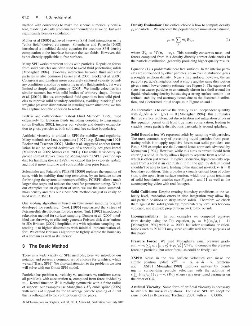
Figures 10 and 11 show selected frames from our 3D simulationresults, referred herein as the “tomato” and the “bunny” examples.Table 1 gives statistics on particle counts, overhead for ghost parti-cles, and run time. The tomato example has a continuous emissionof liquid particles, thus we report average liquid particle count andcomputation time over 16k time steps / 800 frames.

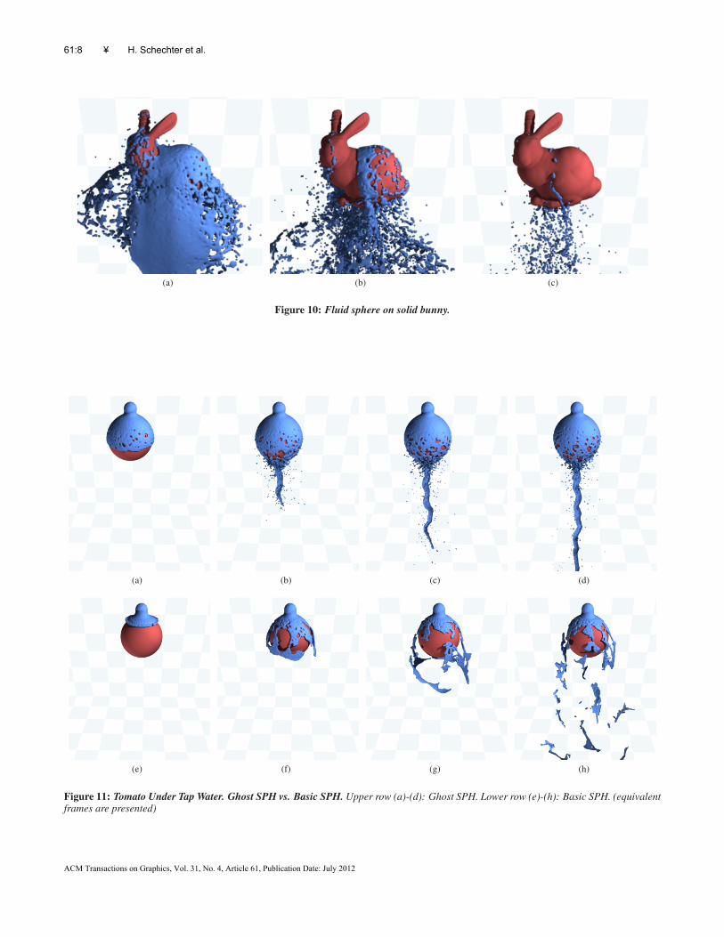
Figure 11 of the tomato example compares Ghost SPH to BasicSPH with the same shared parameters. Basic SPH suffers severesurface tension artifacts at air and solid interfaces, lacks the physi-cal cohesion between liquid and solid, and causes particles to formunnatural clusters instead of spray. Ghost SPH simulation comesmuch closer to the natural motion of the fluid flow (see the video forreal footage), wrapping all the way around the tomato before freelyleaving in a stream from the bottom — despite the small number ofsimulation particles.

The ghost air particles of Ghost SPH added a nontrivial 141%memory overhead in the tomato example, though a much smaller9% overhead for the bunny. Asymptotically the memory overheadscales with the surface area, not the volume, and thus the overheadis reduced at higher resolutions. Interestingly, Ghost SPH only took26% more computation time per time step than Basic SPH for thetomato, 1.29s versus 1.02s: we argue the considerable improve-ment in results at the same resolution is worth this small cost. Thecomputation overhead cause is the air resampling step and the in-creased number of particles; on average air resampling took 11% ofa simulation step computation time, density and particle neighbordata 56%, pressure force 19%, and XSPH for artificial viscosity andboundary conditions took 10% of the time. We also found the im-proved particle distribution at boundaries meant a much wider range



Statistic Tomato Bunny

Liquid particle average count (#) 59k 91kGhost-solid particle overhead 102% 9%Ghost-air particle overhead 136% 40%Avg. computation time per step 1.92 s 1.29sAvg. computation time per frame 38.46 s 25.75s

Table 1: Simulation statistics for the 3D examples. “Overhead”refers to the ratio of ghost particles to real liquid particles. Eachanimation frame is subdivided into 20 time steps.

of stiffness coefficients and artificial viscosities could work, sim-plifying parameter tuning; in some but not all simulations a muchlarger stable time step was possible than with Basic SPH, whichlead to a net improvement in performance.

A larger 750k particle simulation of adouble dam break (frame 250 to the left;also see the accompanying video) aver-aged 21.4s per step, demonstrating theexpected linear cost.

6 Conclusions

Together our ghost treatment of solid and free surface boundaries,particle sampling algorithms, and new XSPH artificial viscosity al-low significantly higher quality liquid simulations than basic SPHwith only a moderate overhead. Our approach should extend easilyto related methods such as PCISPH, and the sampling may find usein any particle simulation. Looking to the future, we plan to extendthe ghost method to a more accurate treatment of surface tensionand to two-way coupling with solids or other fluids.

Acknowledgements

This work was supported in part by a grant from the Natural Sci-ences and Engineering Research Council of Canada and a schol-arship from BC Innovation Council and Precarn Incorporated. Allbunny-like solids were derived from the scanned bunny model madeavailable by the Stanford Computer Graphics Laboratory.

References

ADAMS, B., PAULY, P., KEISER, R., AND GUIBAS, L. J. 2007.Adaptively sampled particle fluids. ACM Trans. on Graphics(Proc. SIGGRAPH) 26, 3.

BATTY, C., BERTAILS, F., AND BRIDSON, R. 2007. A fast varia-tional framework for accurate solid-fluid coupling. ACM Trans.Graph. (Proc. SIGGRAPH) 26, 3.

BECKER, M., AND TESCHNER, M. 2007. Weakly compressiblesph for free surface flows. In Proc. ACM SIGGRAPH / Euro-graphics SCA, 63–72.

BECKER, M., TESSENDORF, H., AND TESCHNER, M. 2009. Di-rect forcing for Lagrangian rigid-fluid coupling. IEEE Transac-tions on Visualization and Computer Graphics 15, 3, 493–503.

BONET, J., AND KULASEGARAM, S. 2002. A simplified approachto enhance the performance of smooth particle hydrodynamicsmethods. Appl. Math. Comput. 126, 2-3, 133–155.

BRIDSON, R. 2007. Fast Poisson disk sampling in arbitrary dimen-sions. In ACM SIGGRAPH Technical Sketches.

CHENTANEZ, N., AND MULLER, M. 2011. A multigrid fluidpressure solver handling separating solid boundary conditions.In Proc. Symp. Comp. Anim., 83–90.

COLAGROSSI, A., AND LANDRINI, M. 2003. Numerical simu-lation of interfacial flows by Smoothed Particle Hydrodynamics.J. Comp. Phys. 191, 2, 448–475.

COOK, R. L. 1986. Stochastic sampling in computer graphics.ACM Trans. Graph. 5, 1.

DUNBAR, D., AND HUMPHREYS, G. 2006. A spatial data struc-ture for fast Poisson-disk sample generation. ACM Trans. onGraphics (Proc. SIGGRAPH) 25, 3.

FEDKIW, R., ASLAM, T., MERRIMAN, B., AND OSHER, S. 1999.A non-osillatory Eulerian approach in multimaterial flows (theGhost Fluid Method). J. Comput. Phys. 152, 457–492.

FEDKIW, R. 2002. Coupling an Eulerian fluid calculation to aLagrangian solid calculation with the Ghost Fluid Method. J.Comp. Phys. 175, 200–224.

GINGOLD, R. A., AND MONAGHAN, J. J. 1977. Smoothed Par-ticle Hydrodynamics - theory and application to non-sphericalstars. Mon. Not. R. Astron. Soc. 181, 375–389.

IHMSEN, M., AKINCI, N., GISSLER, M., AND TESCHNER,M. 2010. Boundary handling and adaptive time-stepping forPCISPH. In Proc. VRIPHYS, 79–88.

KEISER, R., ADAMS, B., GUIBAS, L. J., DUTRE, P., AND PAULY,M. 2006. Multiresolution particle-based fluids. Tech. Rep. 520.

LUCY, L. B. 1977. A numerical approach to the testing of thefission hypothesis. Astron. J 82, 1013–1024.

MONAGHAN, J. J. 1989. On the problem of penetration in particlemethods. J. Comput. Phys. 82, 1–15.

MONAGHAN, J. J. 1994. Simulating free surface flows with SPH.J. Comput. Phys. 110, 399–406.

MONAGHAN, J. J. 2005. Smoothed Particle Hydrodynamics. Re-ports on Progress in Physics 68, 8, 1703–1759.

MULLER, M., CHARYPAR, D., AND GROSS, M. 2003. Particle-based fluid simulation for interactive applications. In Proc. ACMSIGGRAPH / Eurographics SCA, 154–159.

MULLER, M., SOLENTHALER, B., AND KEISER, R. 2005.Particle-based fluid-fluid interaction. In Proc. ACM SIGGRAPH/ Eurographics SCA, 237–244.

SOLENTHALER, B., AND GROSS, M. 2011. Two-scale particlesimulation. ACM Trans. on Graphics (Proc. SIGGRAPH) 30, 4,81:1–81:8.

SOLENTHALER, B., AND PAJAROLA, R. 2008. Density contrastSPH interfaces. In Proc. ACM SIGGRAPH / Eurographics SCA,211–218.

SOLENTHALER, B., AND PAJAROLA, R. 2009. Predictive-corrective incompressible SPH. ACM Trans. on Graphics (Proc.SIGGRAPH) 28, 3.

TURK, G. 1992. Re-tiling polygonal surfaces. ACM Trans. onGraphics (Proc. SIGGRAPH) 26, 2.



(a) (b) (c)

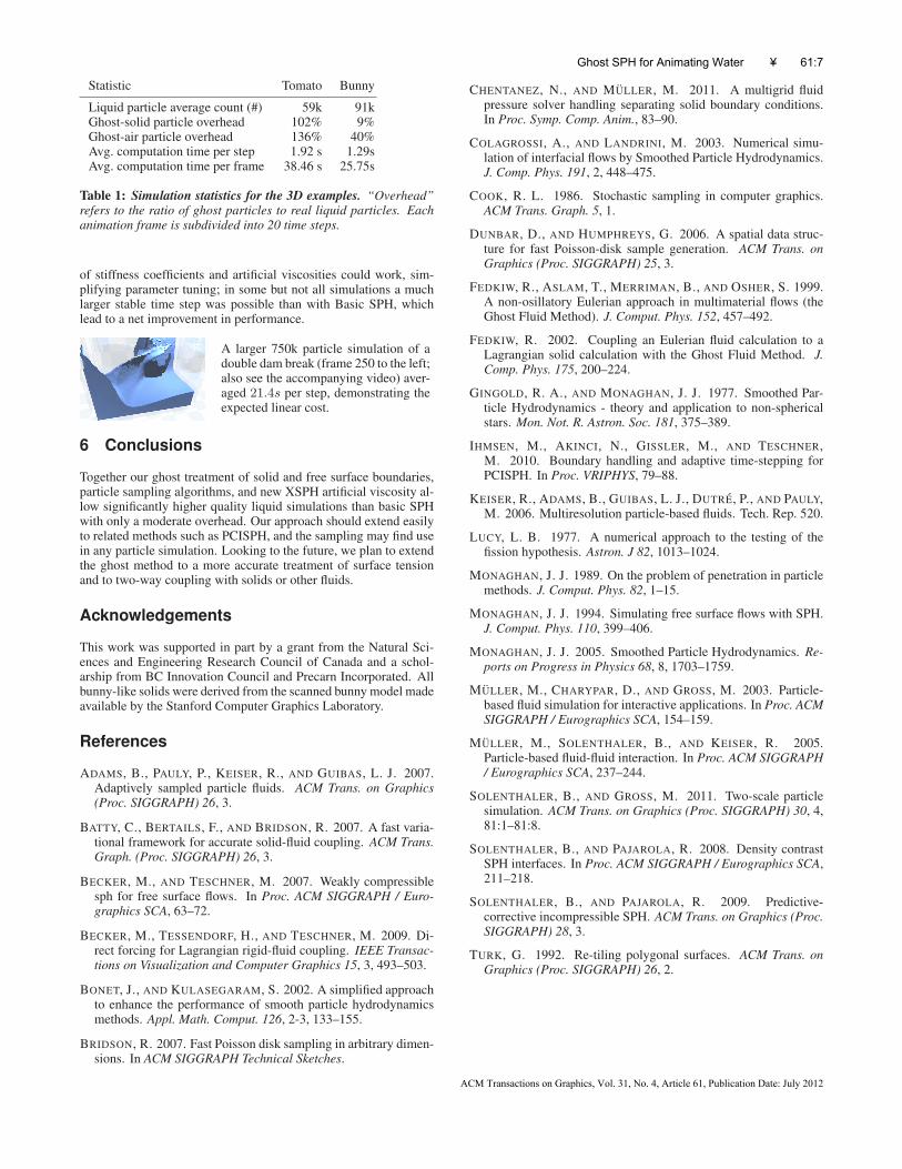
Figure 10: Fluid sphere on solid bunny.

(a) (b) (c) (d)

(e) (f) (g) (h)

Figure 11: Tomato Under Tap Water. Ghost SPH vs. Basic SPH. Upper row (a)-(d): Ghost SPH. Lower row (e)-(h): Basic SPH. (equivalentframes are presented)



schechter siggraph2012 ghostsph

Documents