scattering theory: born series - forschungszentrum...

Scattering Theory: Born Series

Stefan Blügel

This document has been published in

Manuel Angst, Thomas Brückel, Dieter Richter, Reiner Zorn (Eds.):Scattering Methods for Condensed Matter Research: Towards Novel Applications atFuture SourcesLecture Notes of the 43rd IFF Spring School 2012Schriften des Forschungszentrums Jülich / Reihe Schlüsseltechnologien / Key Tech-nologies, Vol. 33JCNS, PGI, ICS, IASForschungszentrum Jülich GmbH, JCNS, PGI, ICS, IAS, 2012ISBN: 978-3-89336-759-7All rights reserved.

A 2 Scattering Theory: Born Series 1

Stefan Blugel

Peter Grunberg Institut andInstitute for Advanced Simulation

Forschungszentrum Julich GmbH

Contents1 Introduction 2

2 The Scattering Problem 22.1 The Experimental Situation . . . . . . . . . . . . . . . . . . . . . . . . . . . . 32.2 Description of Scattering Experiment . . . . . . . . . . . . . . . . . . . . . . 42.3 Coherence . . . . . . . . . . . . . . . . . . . . . . . . . . . . . . . . . . . . . 72.4 The Cross Section . . . . . . . . . . . . . . . . . . . . . . . . . . . . . . . . . 8

3 Lippmann Schwinger Equation 9

4 Born Approximation 114.1 Example of Born Approximation: Central Potential . . . . . . . . . . . . . . . 124.2 Example of Born Approximation: Square Well Potential . . . . . . . . . . . . 134.3 Validity of first Born Approximation . . . . . . . . . . . . . . . . . . . . . . . 144.4 Distorted-Wave Born Approximation (DWBA) . . . . . . . . . . . . . . . . . 15

5 Method of Partial Wave Expansion 175.1 The Born Approximation for Partial Waves . . . . . . . . . . . . . . . . . . . 205.2 Low Energy Scattering: Scattering Phases and Scattering Length . . . . . . . . 215.3 S-Wave Scattering at Square Well Potential . . . . . . . . . . . . . . . . . . . 225.4 Nuclear Scattering Length . . . . . . . . . . . . . . . . . . . . . . . . . . . . 25

6 Scattering from a Collection of Scatterers 25

1Lecture Notes of the 43rd IFF Spring School “Scattering Methods for Condensed Matter Research: TowardsNovel Applications at Future Sources” (Forschungszentrum Julich, 2012). All rights reserved.

A2.2 Stefan Blugel

1 Introduction

Since Rutherford’s surprise at finding that atoms have their mass and positive charge concen-trated in almost point-like nuclei, scattering methods are of extreme importance for studyingthe properties of condensed matter at the atomic scale. Electromagnetic waves and particleradiation are used as microscopic probes to study a rich variety of structural and dynamicalproperties of solids and liquids. Atomistic processes in condensed matter take place at lengthscales on the order of an Angstrom (1A= 10−10m) and an energy scale between a meV and afew eV. Obviously, detailed information concerning atomic systems require measurements re-lated to their behavior at very small separations. Such measurements are in general not possibleunless the de Broglie wavelength (λ = h

p= h

mv) of the relative motion of the probing particle is

comparable to these distances. This makes x-ray scattering and neutron scattering, in additionto electron scattering and to a certain extent also Helium scattering, to the outstanding micro-scopic “measurement instruments” for studying condensed matter. To push electromagneticwaves in this area one uses either x-rays with wavelengths of a few Angstroms, but in the keVenergy range, or light with energies in the eV range, but wavelengths of some 1000 A. Neutrons(and Helium atoms) make it possible to match energy and wavelengths simultaneously to thetypical atomic spacings and excitation energies of solids (solid surfaces). Thus, a simultaneousspatial and temporal resolution of atomistic or magnetic processes is possible. In addition, thephoton, neutron, electron and under certain conditions also Helium possess internal degrees offreedom such as a polarization vector or a spin with which the probes couple to core and va-lence electrons. The photon, neutron and Helium result in only week interaction with matter,which simplifies considerably the analysis and interpretation of experiments as multiple scatter-ing processes are frequently of minor importance and can often be ignored completely, whichmakes an interpretation of the scattering results valid within a kinematic scattering theory.In this Chapter, we will provide a brief introduction to the elementary concepts and methodol-ogy of scattering theory. The focus lies on the introduction of the description of the scatteringprocess in terms of the Hamiltonian of the scattering projectile at a finite range interaction poten-tial of a single site target by the method of partial waves, i.e. using differential equation methodsand the Lippmann-Schwinger equation, i.e. using an integral equation formulation of scatteringthat leads then to the first Born approximation of scattering and the distored wave Born ap-proximation. The former is the approximation of choice if multiple scattering is unimportantand the latter is applied in the analysis of grazing-incidence small-angle scattering experimentsdiscussed in more details chapter D2. The lecture closes with the discussion of the scatteringon the lattice rather than a single site target resulting briefly the Bragg scattering, that will bediscussed in more detail in the lecture Scattering Theory: Dynamical Theory (A3). The subjectis typically part of an Advanced Quantum Mechanics curriculum and is therefore elaborated attextbooks on quantum mechanics. A selection is given as references [1, 2, 3, 4].

2 The Scattering Problem

In a scattering experiment a beam of particles is allowed to strike a target,2 and the particles thatemerge from the target area or scattering volume, respectively, are observed.

2In the language of elementary scattering theory one frequently refers to a target although we keep in mind thatin the language of condensed matter, it is referred to as the sample.

Basic Scattering Theory A2.3

z-axisCollimatorTarget

Θ

Source

Detector

Fig. 1: A set-up of a typical diffraction experiment consisting of a particle source, a scatteringtarget and a particle detector. The beam passes through a collimator with an beam opening ∆r.

2.1 The Experimental Situation

A schematic representation of a standard scattering experiment appears in Fig. 1. Each scat-tering experiment consists of three indispensable elements: (i) The source of incident beam ofparticles or electromagnetic wave, to propagate with wave vector k = 2π

λk of wavelength λ

along the direction k, which we assume without loss of generally to be the z-direction (the axisof the collimator). (ii) The target, that we consider stationary, a reasonable assumption in con-densed matter physics and (iii) the detector, whose function is to simply count the number ofparticles of a particular type that arrive at its position r with the coordinate r = (x, y, z) in realspace along the direction r at the angle (θ, ϕ) with respect to the axis of the propagating incidentbeam. Ideally it may be set to count only particles of a given energy, spin or polarization vector,respectively. We assume throughout that the source and detector are classical objects that havea clearly defined, precisely controllable effect on the scattering process. The detector will beassumed to be 100% efficient and to have no effect on the scattered particle prior to the time itenters the detector.The result of the scattering experiment will vary with the energy E of the incident beam. In or-der to simplify the analysis of the experimental data, the energy spectrum of the incident beamshould be sharply peaked so that the experiment may be considered to take place at a unique en-ergy eigenvalue E. To this end, in most experiments care is taken to achieve a monochromaticincident beam characterized by the wave vector k. We shall assume here that the beam emerg-ing from the collimator is both perfectly monochromatic and perfectly collimated, as well. Ofcourse, according to the uncertainty principle, a beam of finite cross section (of the size of thecollimator opening ∆r) cannot be perfectly monochromatic (∆k > 0) and perfectly collimatedas well. We may, however, assume the beam to be sufficiently well collimated that the angulardivergence may be ignored in an actual experiment. In that case we must necessarily have not amonochromatic beam represented by a plane wave, but rather a beam describable as a superpo-sition of such waves. In this respect the collimator can be considered the fourth indispensableelement of a scattering experiment. It shields the detector from the incoming beam to the idealextent that no count is measured in the detector without target, and produces a small beam ofmonochromatic energy. We further assume that the detector has a small opening angle dΩ andis positioned at large distance from the target. Under these conditions, the scattered beam can becharacterized at the position of the detector by the wave vector k′ and energy E ′. Summarizing,in a scattering experiment a wave packet of incident particles characterized by the initial state(k, E, e), denoting the polarization vector e of an x-ray beam as a representative of an internal

A2.4 Stefan Blugel

Target

θ

φ

x-axis

y-axis

z-axis

Detector

k

incident beam(E,k, e)

k′

scattered beam(E ′,k′, e′)

r2dΩr

Fig. 2: The geometry of the scattering experiment.

degree of freedom of the particle, is scattered into the final state:

(k, E, e)scattering−→ (k′, E ′, e′). (1)

The scattering process is characterized by the scattering vector

Q = k′ − k (2)

and the energy transition~ω = E ′ − E. (3)

~Q represents the momentum transfer during scattering, since according to de Broglie, the mo-mentum of the particle corresponding to the wave with wave vector k is given by p = ~k. Forelastic scattering (diffraction), it holds that E ′ = E and |k′| = |k| and all possible scatteringvectors are located on a sphere, called Ewald-sphere. Structural investigations are always car-ried out by elastic scattering. The magnitude Q of the scattering vector can be calculated fromwavelength λ and scattering angle θ as follows

Q =√k2 + k′2 − 2kk′ cos θ =

√2k2(1− cos θ) = k

√2(1− cos2

θ

2+ sin2 θ

2) =

4π

λsin

θ

2(4)

2.2 Description of Scattering ExperimentAfter the beam of particles is emitted from the collimated source, the experimenter has nocontrol over the particles until they have reached his detector. During that time, the propagationis controlled solely by the laws of quantum mechanics and the Hamiltonian of the projectile-target system. We restrain our description to the nonrelativistic domain and may thus formulatethe physical situation in terms of the solution of a Schrodinger equation using an appropriate


Hamiltonian and suitable boundary conditions. The occurring phenomena can be very complex.We assume in the following that the incident particles do not interact with each other duringthe time of flight, rather that the particles fly one by one, and that incident particles and thetarget particles do not change their internal structures or states, but only scatter off each other.Internal excitations, rearrangements, charge or spin exchange are also excluded. In fact, internaldegrees of freedom such as the spin or polarization vector are currently completely neglected.That means we shall consider only the purely elastic scattering. We further neglect the multiplescattering in the target and consider at first only the interaction of an incident particle with onetarget particle, the state of both is described by a two-particle wave function Ψ(rP, rT) and theinteraction is described by a potential V (r) which depends only on the relative distance r = rT−rP, where the subscripts T and P denote the target and the incoming particle, respectively. Weshall confine ourselves in this article to scattering processes in which only short-range centralforces are present. In the presence of such potentials, the particle is not under influence of thetarget potential when they are emitted from the source or when they enter the detector. Sincefor the two-body problem the motion of the center of mass R can be separated out, the problemreduces to the scattering of a particle with the reduced mass 1

m= 1

mT+ 1

mPat the potential

V (r). Since the potential does not depend explictly on the coordinate of the center of mass R,the two-particle wave function can be expressed in terms of a product of single-particle wavefunctions Ψ(rP, rT) = φ(R)ψ(r),3 both solutions of two separate Schrodinger equations. Theelementary two-body scattering process could be intrinsically elastic, but recoil of the targetparticle might lead to a transfer of energy to the target. In the present context elastic scatteringspecifically excludes such effects. Considering a solid as target, depending on the energy ofthe projectile and the interaction of the constituent atoms in a solid, this can be a very goodassumption, as for favorable circumstances all atoms contribute to the scattering mass of thesolid (of course, in other chapters it becomes clear that atoms in a solid vibrate and a scatteringevent may cause inelastic excitations of phonons in the vicinity of the elastic energy). To thinkthat the target particle or a target solid is infinitely heavy relative to the mass of the incidentparticle simplifies our thinking further. In this case the center of mass of the target remainsstationary at the position of the target particle throughout the scattering process. Under thesecircumstances the relative coordinate r represents the actual laboratory coordinate of the lightparticle and the mass m is then the mass of the incident particle. These parameters enter thetime-dependent Schrodinger equation

i~∂ψ

∂t=

[− ~2

2m∇2 + V (r)

]ψ with V (r) = 0 except r ∈ target region T (5)

to be solved.The time-dependent Schrodinger equation seems a natural starting point for the descriptionof a scattering event as it is not a stationary process but involves individual discrete particlesas projectiles, but as we see a bit later the good news is, that under reasonable assumptionsthat are fulfilled in typical experimental situations, the same results are obtained using a time-independent description applying the stationary Schrodinger equation.At the vicinity of the collimator and detector, the solution of the potential-free Schrodingerequation (5) is analytically known as the free-particle wave packet:

ψ(r, t) =1

(2π)3

∫d3k A(k)ψk(r, t) with ψk(r, t) = eikre−i

~k22m

t. (6)

3This does not hold if target and projectile are identical particles. Identical articles scattering about angle θ andπ − θ cannot be distinguished.

A2.6 Stefan Blugel

The wave packet is expressed as a superposition of a complete set of stationary-state solutionsψk(r) of this Schrodinger equation, which are plane waves ψk(r) = eikr. The energy eigenvaluecorresponding to the eigenfunction ψk is simply Ek = ~2

2mk2. For convenience the target is

placed at the origin of the coordinate system (r = 0). The coefficient A(k) is the probabilityamplitude for finding the wave number k, or momentum ~k in the initial state. We assumethat the properties of the source are such that the wave packet is close to monochromatic andthat the amplitude function A(k) peaks about the average momentum ~k = ~k with a spreadin the wave number ∆k that is small compared to k (∆k k), related to the opening ofthe collimator ∆r by Heisenberg’s uncertainty principle (∆k∆r ' 1). If we finally imposethe condition (∆k)2

kL 1 (equivalent to the condition λ

∆r ∆r

L) the packet does not spread

appreciably during the course of the experiment with the set-up of length L, and we can finallyshow that a stationary description of the scattering problem is sufficient. Under these conditionsthe energy-dependent phase factor of ψk(r, t) can be conveniently be approximated about themedian energy k2 ' −k2

+ 2k · k and Eq. (6) will become

ψ(r, t) = ei~k22m

t 1

(2π)3

∫d3k A(k) eik·(r−vt) = ei

~k22m

tψ(r− vt, 0), (7)

i.e. a wave packet ψ(r, t) centered about the origin r = 0 at t = 0 moves at the classicalvelocity v = ~k

mand the packet at time t > 0 will have exactly the same shape, but centered

about r = vt. Thus, the initial state limt→−∞ ψ(r, t) and the final state limt→+∞ ψ(r, t) canbe expressed by Eq. (7), but with the coefficients A(k) in the final state having been modifiedcompared to the ones in the initial state due to the scattering, as we shall discuss immediately.A solution of Eq. (5) requires, however, the specification of boundary conditions imposed onthe solution that reflect the physical situation in the laboratory as discussed in section 2.1. Theproper boundary condition is a condition on the wave function when the particle and target arefar apart. It can be motivated from Huygens’ principle [5] who proposed that every point whicha luminous disturbance reaches becomes a source of a spherical wave, and the sum of thesesecondary waves determines the form of the wave at any subsequent time. For a single targetscatterer we express the wave function

ψk(r)r→∞−→ eikr +

1

reikrfk(θ, φ) ∀k and t > 0 (8)

in terms of a superposition for the incoming wave plus an outgoing scattered wave emanatingfrom the target, removing some of the incoming particles from the incident primary beam.f(θ, φ), f(r) or f(k′), respectively, denotes the scattering amplitude. This form of the wavefunction is motivated by the fact that we expect, after scattering, an outgoing spherical wave,modified by the scattering amplitude, interfering with the incoming wave; we will later show amore rigorous justification of this expression. Consistent to the lab schematics in Fig. 1, k‖zand the azimuthal and polar scattering angle (θ, φ) are given by the projection of the direction ofthe wavevector k of the scattered wave, e.g. into the detector at direction r and the z direction.If we replace ψk(r, t) in (6) by its asymptotic form given in (8), when the packet is far fromthe target, the wave function ψ′(r, t) (where we use a prime to denote the wave function afterscattering) breaks up into two terms

ψ′(r, t) = ψk(r, t) + ψsc(r, t), with ψsc(r, t) = 0 for t < 0 (9)

with the incident beam ψk(r, t) identical to Eq. (7) and the scattered wave ψsc(r, t) according


to Eq. (6)

ψsc(r, t) =1

r

1

(2π)3

∫d3k fk(r)A(k) eikr e−i

~k22m

t. (10)

If we assume now that the scattering amplitude is slowly varying over the spread of the wavenumbers ∆k, and thus approximate fk(r) ' fk(r) as well as making use of the approximations

k ' k · k and k2 ' −k2 + 2k · k for (∆k)2 k2

(11)

(k = |k| = |k+∆k| = [k2+2k ·∆k+(∆k)2]1/2 ' k[1+2k ·∆k/k2

]1/2 ' k+k ·(k−k))

in which k is equal to the projection along k we obtain

ψsc(r, t) = e−i~k22m

t 1

rfk(r)

1

(2π)3

∫d3k A(k) eik·(kr−v t) = e−i

~k22m

t 1

rfk(r)ψ(kr−vt, 0) .

(12)Thus, after the incident packet has passed the target a spherical scattered wave shell of thickness∆r, equal to the size of the packet, centered on the origin and having a radius r = vt emergesfrom the target. One finds further that the incoming wave packet given in (7) and the scatteredwave, Eq. (12), share absolutely the same time dependence and are the same for all k. Thesolution is actually a superposition of all available wave numbers according to

∫d3kA(k) . . . .

Since there is no mode-mode coupling such as k → k1 + k2, it is totally sufficient to solvethe problem in terms of a scattering problem of ψk(r) on the basis of a stationary Schrodingerequation for all relevant wave vectors k, which will be pursued during the rest of the manuscript,and keep thereby in mind that a wave packet is formed with a certain probability amplitude. Thisstationary problem with plane waves as incident beam simplifies the description of scatteringsignificantly.

2.3 CoherenceThe formation of a wave packet bears, however, a consequence on which we shall briefly touchupon: The scattering pattern or diffraction pattern, respectively, will be a superposition of pat-terns for different incident wave vectors (k,k+∆k) and the question arises, which informationis lost due to these non-ideal conditions. This “instrumental resolution” is intimately connectedwith the “coherence” of the beam and the size of the scattering volume in comparison to the tar-get volume. Coherence is needed, so that the interference pattern is not significantly destroyed.Coherence requires a phase relation between the different components of the beam. A measurefor the coherence length l is given by the distance, at which two components of the beam be-come fully out of phase, i.e. when one wave train at position r exhibits a maximum, meats awave train exhibiting a minimum, thus experiencing a phase difference of λ/2. If the coherencelength l‖ is determined by the wavelength spread, λ and λ + ∆λ one refers to the temporal orlongitudinal coherence. The condition l‖ = nλ = (n− 1

2)(λ+ ∆λ) translates then into

l‖ =1

2

λ2

∆λfor longitudinal coherence

and

l⊥ =1

2

λ

∆θfor transversal coherence.

A2.8 Stefan Blugel

Analogously one obtains the transversal coherence length l⊥ shown in above equation due tothe divergence of the beam ∆θ that results from the finite transverse beam size due to thefinite extension of the source. In many instruments, the vertical and horizontal collimations aredifferent and the vertical one can even be different along different spatial directions.Together, the longitudinal and the two transversal coherence lengths define a coherence volume.This is a measure for a volume within the sample, in which the amplitudes of all scatteredwaves superimpose to produce an interference pattern. Normally, the coherence volume issignificantly smaller than the sample size, typically a few 100 A for neutron scattering, up to µmfor synchrotron radiation. Scattering between different coherence volumes within the sampleis no longer coherent, i.e. instead of the amplitudes, the intensities of the contributions to thescattering pattern have to be added. This limits the spatial resolution of a scattering experimentto the extension of the coherence volume.

2.4 The Cross Section

A general measure of the scattered intensity I(Ω) is the differential cross section ( dσdΩ

). It isdefined by the number of particles dN counted per unit time dt scattered into a cone of solidangle dΩ = sin θ dθ dφ in the detector located at the distance r along a ray specified by thedirection r, at angle (θ, φ) or the solid angle Ω, respectively, normalized to the current of theincoming particles jin

1

jin

dN

dt=

(dσ

dΩ

)dΩ =

(dσ

dΩ

)1

r2dA. (13)

dσ describes a cross-sectional area with a surface normal parallel to k, through which thenumber of particles dN that get scattered into the angle Ω flow per unit time. The total crosssection

σtot =

∫ 4π

0

(dσ

dΩ

)dΩ (14)

is the total effective geometrical cross-sectional area of the incident beam that is intercepted andthe particles therein deflected by the target object.From Eq. (13) the scattered current density is jsc = 1

r2jin( dσ

dΩ). On the other hand jsc can be

calculated directly employing the expression of the probability current density given by

jsc(r) = −i ~2m

[ψ∗sc(r)∇ψsc(r)− ψsc(r)∇ψ∗sc(r))] ' jin1

r2|f(Ω)|2 r +O

(1

r3

). . . (15)

where as ψsc = 1reikrf(Ω) is the asymptotic scattering wave, Eq. (8). We explicitly inserted

here the current density jin = ~km

to the incoming plane wave ψin. Equating the two expressionsgives the relation

I(Ω) ∝(dσ

dΩ

)= |f(Ω)|2 (16)

for the differential cross section. This expression relates the experimental quantity, the differ-ential cross section, to the scattering amplitude, which characterizes the wave function at largedistances from the target. It is the fundamental relation between scattering theory and scatteringexperiments.


3 Lippmann Schwinger EquationHaving established the basic concepts for the scattering problem, we turn now to the illustrationof the physical ideas that underlie the scattering analysis using integral equation methods. Werecall that we are looking for the solution of the stationary Schrodinger equation[− ~2

2m∇2 + V (r)

]ψk(r) = Eψk(r) with V (r) = 0 except r ∈ target region T,

(17)that is consistent with the boundary condition (8) of an incident plane wave ψk(r) = eikr andan emanating scattered wave. The energy E is determined by the energy of the incident planewave Ek = ~2

2mk2. By introducing the Green function G,[

~2

2m∇2 + E

]G(r, r

′|E) = δ(r− r′), (18)

for the potential-free Schrodinger equation, the Schrodinger equation for ψk(r),[~2

2m∇2 + E

]ψk(r) = V (r)ψk(r), (19)

can be transformed into an integral equation

ψ′k(r) = ψk(r) +

∫Td3r′G(r, r

′|E)V (r′)ψ′k(r′), (20)

in which the formal expression V (r)ψ′k(r) is conceived as inhomogeneity of the differentialequation (18). This integral equation is called the Lippmann-Schwinger equation. Hereby,ψk(r) is the above cited plane-wave solution of the potential-free Schrodinger equation. Theindex k in ψ′ expresses the fact that this state has evolved from one that in the remote past was aplane wave of the particular wavevector k. Obviously, in the limit of zero potential, V (r)→ 0,the scattered and the incident wave are identical, ψ′k(r) = ψk(r).The Green function G(r, r′|E) is not uniquely determined by the Schrodinger equation (18).Also here the unique solution requires a boundary condition, which is chosen such, that thesolution ψ′k(r) describes outgoing scattered waves. The Green function G(r, r′|E),

G(r, r′|E) = −2m

~2

1

4π

eik|r−r′|

|r− r′|with k =

√2m

~2E, (21)

describes then the stationary radiation of a particle of energy E, that is generated at r′, by aspherical wave outgoing from the target. In other words, the Green function G(r, r′|E) givesthe amplitude of this wave at location r due to its generation by the source at r′, under thecondition that the wave is not further scattered during its propagation from r′ to r. By theLippmann-Schwinger equation, the incident wave ψk(r) is superimposed with spherical wavesemitted from scattering at position r′ in the target. The amplitude of these scattered waves isproportional to the interaction potential V (r′) and the amplitude of the total wave field ψ′(r′) atthat point.Recalling our experimental set-up that the distance between target and detector is significantlylarger than the size of the sample, for large distances between r and the scattering center r′

A2.10 Stefan Blugel

it is useful to expand the Green function G in powers of r′

r 1 assuming that the extent

of r′ is restricted to the space of a small target or scattering volume, respectively, r′ ∈ T.Approximating for r′ r

1

|r− r′|=

1

r+O

(1

r2

)and |r− r′| ≈ r − r · r′ with r =

r

r(22)

and inserting this into the relation (21) one obtains the asymptotic form, or far-field limit, re-spectively, of the Green function G,

G(r, r′|E) = −2m

~2

1

4π

eikr

re−ikr·r

′+ O

(1

r2

). (23)

Inserting this expression into the Lippmann-Schwinger equation (20) one obtains the asymptoticsolution of the wave function ψ′k(r) for large distances r

ψ′k(r) ' eikr +1

reikrfk(r), (24)

which is exactly the boundary condition (8) we conjectured from Huygens’ principle, whereasthe scattering amplitude f(r) = f(θ, φ) is given by the integral,

fk(r) = −2m

~2

1

4π

∫d3r′ e−ik

′r′V (r′)ψ′k(r′) = −4π~2

2mT (k′,k) (25)

that can be interpreted as a transition-matrix element from the scattering state described byψ′k(r′) to the scattered state at far distances, which is a plane-wave state described by k′ =k · r, the wave vector of the scattered wave in the direction of the detector, which is knownin the experiment. T (k′,k) is referred to as the T matrix or transition amplitude, a quantityproportional to the scattering amplitude. Due to the far-field approximation (22) the scatteringpattern fk(r) is independent of the distance between target and detector, depending only on theangles to the detector from the target. In optics this is known as the Fraunhofer diffraction andin this context approximation (23) is also referred to as the Fraunhofer approximation of theGreen function.

scattering volume

Detector

k

k′‖rr′

r− r′

Fig. 3: Scattering geometry for the calculation of the far-field limit at the detector. In theFraunhofer approximation, we assume that |r| |r′|.


4 Born ApproximationNote that in the Lippmann-Schwinger equation (20) the wave function ψ′(k) appears both onthe left and right hand side. In a general case, there is no simple way to find exact solutions ofthe Lippmann-Schwinger equation. The form of the Lippmann-Schwinger equation provides anatural but approximate means that can be used for any potential, under the proper conditions,to proceed by an iterative procedure. At zeroth order in V , the scattering wave function isspecified by the unperturbed incident plane wave,

ψ′(0)k (r) = eikr. (26)

Then one can iterate the Lippmann-Schwinger equation (20) according to the rule

ψ′(n+1)k (r) = eikr +

∫d3r′G(r, r

′|E)V (r′)ψ′(n)k (r′) (27)

that results in the Born expansion of the wave function in powers of the interaction potential Vwritten here in a symbolic form4

ψ′k = ψ′(0)k + ψ

(1)k + ψ

(2)k + ψ

(3)k + · · ·+ (28)

= ψ′(0)k +GV ψ

′(0)k +GV GV ψ

′(0)k +GV GV GV ψ

′(0)k + · · ·+ (29)

= (1 +GT )ψ′(0)k with T = V +GV + · · ·+ =

1

1− V G(30)

k

k′+

k

k′+

k

k′+ . . .

A term-by-term convergence of this series is in general not guaranteed and depends on thepotential and the energy of the incident particle, even though the final expression is alwaysvalid. Physically, an incoming particle undergoes a sequence of multiple scatteringevents from the potential. The first term in the series expansion (29) de-

kk′

scribes single scattering processes of the incident wave, while the follow-ing terms describe then scattering processes of successively higher order.Rarely are higher-order terms calculated analytically, since the complica-tions then become so great that one might as well use a numerical methodto obtain the exact solution if this is possible at all. Thus, only the firstiteration of the series is taken into account, i.e. only single scattering, andthe T matrix is approximated by the potential matrix V (k′,k),

T (k′,k) ' V (k′,k). (31)

This first order term, in which the exact wave function ψ′k(r′) in the integral kernel is replacedby the plane wave eikr′ is the first Born approximation and typically abbreviated as the Bornapproximation.5 This approximation is most useful when calculating the scattering amplitude.

4Please note that ψ(n)k = (GV )nψ′(0)k . This is different from definition ψ′(n)

k (r) in (27).5It should not be confused with the Born-Oppenheimer approximation.

A2.12 Stefan Blugel

In first Born approximation the general equation for the scattering amplitude (25) reads then

f(1)k (r) = −2m

~2

1

4π

∫d3r′ e−ik

′r′V (r′) eikr′ = −2m

~2

1

4πV (Q) with Q = k− k′, (32)

with V (Q) denoting the Fourier transform of the potential with the momentum transfer Q.6

V (Q) can be interpreted as a transition-matrix describing the transition from the incomingplane-wave of state k into the outgoing plane-wave state k′ due to the action of the potentialexpressed in the reciprocal space at scattering angle Q. From (16) follows then the differentialcross section (

dσ

dΩ

)(1)

=

(2m

~2

)2π

2|V (Q)|2. (33)

The physics behind the 1st Born approximation is provided by the assumption that the incomingwave scatters only once inside the target potential before forming the scattered wave ψ(1). Thisis the concept behind the kinematic theory of scattering, that simplifies the interpretation ofthe scattering experiment substantially. For example, for the case of elastic scattering that weassumed all the time during the derivations, energy is conserved |k|2 = |k′|2, all possiblescattering vectors are placed on the so-called Ewald sphere with radius |k|. The length ofthe scattering vector Q is then given by

Q(Ω) = |Q| = 2 |k| sin1

2Ω =

4π

λsin

1

2Ω with Ω = (θ, φ)^(k′,k). (34)

Note, and this is the essence of the Ewald-sphere, that this shows Ewald sphere|k| = |k′|

k

k′ Q

θ

Fig. 4: The Ewald sphere.

that the differential cross section (33) does not depend on scat-tering angle and beam energy independently, but on a single pa-rameter through the combination Q = 2k sin 1

2Ω. By using a

range of energies, k, for the incoming particles, this dependencecan be used to test whether experimental data can be well de-scribed by the Born approximation. A very common use of theBorn approximation is, of course, in reverse. Having found dσ

dΩ,

experimentally, a reverse Fourier transform can be used to obtain the form of the potential.

4.1 Example of Born Approximation: Central PotentialFor a centrally symmetry potential, V (r) = V (r), we can make some progress with the matrixelement integral (32) if we choose a polar coordinate system with Q along the z-axis, so thatQ · r = Qr cos θ. Then, the scattering amplitude in Born approximation f (1)(θ) is written aftersome manipulations in the form

f(1)k (θ) = −2m

~2

1

Q

∫ ∞0

V (r) r sinQr dr (35)

and is seen to be independent of φ due to the cylindrical symmetry of the problem at hand andall scattering vectors are placed on an Ewald-circle. An example, is the Rutherford scatteringor Coulomb scattering, respectively, where a charged particle with charge Z1e impinges on an

6It would be mathematically more correct to denote the Fourier transformationF of V (r) by a different functionname e.g. V (Q) = F [V (r)]. To avoid incomprehension of reading due to unduly complicated notation we replaceV (Q) by V (Q).


other charged particle with charge Z2e under the action of a Coulomb potential, which resultsinto the scattering amplitude

f(1)k (θ) = −2m

~2

Z1Z2

Q2e2 = −1

4

Z1Z2

sin2 12θ

e2 1

E(36)

and the differential cross section,(dσ

dθ

)(1)

=

∣∣∣∣14 Z1Z2

sin2 12θ

e2

∣∣∣∣2 1

E2(37)

known as the Rutherford formula. Due to the long-range nature of the Coulomb scatteringpotential, the boundary condition on the scattering wave function does not apply. We can, how-ever, address the problem by working with the screened (Yukawa) potential, V (r) = Z1Z2

re−κr,

leading to f (1) ∝ 1Q2+κ2 and taking κ→ 0, which leads then to the Rutherford formula (37). Ac-

cidentally, the first Born approximation gives the correct result of the differential cross sectionfor the Coulomb potential.

4.2 Example of Born Approximation: Square Well PotentialConsider scattering of particles interacting via a spherical three dimensional (3D) square wellpotential V (r) = V for r ≤ R and zero outside (V (r) = 0 for r > R). The integral (35) forthe scattering amplitude required here is then

f(1)k (θ) =

2m

~2

1

Q

∫ R

0

V r sinQr dr =2m

~2

1

QV

[sinQr −Qr cosQr

Q2

]R0

(38)

7 and whence to the differential cross section(dσ

dθ

)(1)

=

(2m

~2

VQ

)2

R2 j

21(QR) '

(2m

~2

VQ

)2

19

(1− 1

5Q2R2

)

for low E, kR < 1R2

Q2 for high E, kR > 1.

(39)From integrating over θ and φ the low and high energy limits for the total cross section are

σ(E →∞) = π

(2m

~2

)2(VR

3

kR

)2

σ(E → 0) = σ(E →∞)8

9

(k2R2

−2

5k4R4

+ · · ·).

(40)The two examples illustrate some general features of scattering in the Born approximation:(i) Born approximation is based on perturbation theory, so it works best for high energy parti-cles.(ii) At high energy, the scattering amplitude and the cross section are inversely proportionalto the energy (E = ~2k2/2m). E.g. both become smaller and the scattering weaker withincreasing energy. This is a general phenomenon, if no bound states appear in the vicinityof the energy. This can be seen best by inspecting the Fourier transformed Green functionG(k|E) ∝ 1/(E − h2k2

2m) that is inverse proportional to the energy.

(iii) Scattering depends on square of the interaction potential, e.g. V 2 , so both attractive and

7j0(Qr) = sinQr/Qr is the spherical Bessel function for angular momentum ` = 0. Radial integration leadsto Bessel function j1(Qr).

A2.14 Stefan Blugel

repulsive potentials behave the same.(iv) The dependence on the energy of the incident beam k and scattering angle θ arises onlythrough the combination Q = 2k sin θ

2. Thus as energy increases, the scattering angle θ is re-

duced and the scattered beam becomes more peaked in the forward direction.(v) Angular dependence depends on the range of the potential R but not on the strength V.(vi) The total cross section depends on both range R and depth V of the potential.

4.3 Validity of first Born ApproximationThis raises the practical questions (i) under which conditions the Born expansion converges and(ii) whether the first term is a good approximation. In the Born approximation the T matrix isapproximated by the potential matrix V . This will not work if the denominator |1 − V G| in(30) is small or zero. This is the situation at low energy, when the energy of the incoming beamcoincides with bound states of the potential. Then, the Born approximation is invalid and theBorn expansion will not converge. The solution to this problem is provided by the dynamicalscattering theory discussed in Chapter A3. According to (30) the Born approximation T ' Vis equivalent to the condition∣∣∣∣∫ ∫

Td3r d3r′ V (r)G(r, r

′|E)V (r′)

∣∣∣∣ 1 . (41)

At the same time this condition determines the radius of convergence of the Born series withrespect to the strength of the potential. This condition means that the first Born approximationis valid and the Born series converges if the potential is sufficiently weak and the approximationimproves as the energy is increased. Concerning the question whether the first term is itself agood approximation to the wave function, a convenient, although nonrigorous, criterion can beobtained by requiring that the first-order correction to the wave function be small compared tothe incident wave in the region of the potential, i.e. |ψ′(1)

k (r)| |ψ′(0)k (r)| which results to

2m

~2

1

4π

∣∣∣∣∫Td3r′ e−ikr

′V (r′) e−ikr′

∣∣∣∣ 1. (42)

For the above introduced spherical 3D square well potential V (r ≤ R) = V and V (r > R) =0, this implies ∣∣∣∣mV~2k2

(eikR sin kR − kR

)∣∣∣∣ 1. (43)

orm

~2|V|R2

1 for low energies kR < 1 (44)

m

~2|V|R

1

k 1 for high energies kR > 1. (45)

Since a bound state for this potential exists when m~2 |V|R2

& 1, as said above, the Born ap-proximation will not be valid at low energies if the potential is so strong that it has a boundstate. On the other hand criterion (45) can be satisfied for any potential by going to sufficientlyhigh energy. When we square criterion (45) and multiply it by the geometrical cross sectionσgeo = πR2

, criterion (45) reads

π

(2m

~2

)2(VR

3

kR

)2

πR2 ⇐⇒ σtot σgeo. (46)


and provides a hand-waving criterion when the potential is sufficiently weak so that the Bornapproximation gives reliable results: If the ratio of the scattering cross section and the geomet-rical extension of the potential is small, u := σtot

σgeo 1, the Born approximation can be used.

For x-ray and neutron scattering, the scattering cross sections amount to a few 10−24 cm2, thecross-sectional area per atom is of the order of several 10−16 cm2. This results indeed in a verysmall potential strength of u ∼ 10−8 ÷ 10−7 for scattering on different atoms: that means, theBorn approximation is justified and the easy-to-interpret kinematic interpretation of scatteringresults is sufficient. The arguments become invalid for the nuclear scattering of neutrons byindividual nuclei as the cross-sectional area of a nucleus is eight orders of magnitude smallerand the scattering cross section and the geometrical gross section can be of similar size and thepotential strength u can be even larger than 1, u > 1. Due to the strong Coulomb interactionpotential, the probability for multiple scattering processes of electrons in solids is extremelyhigh, making the interpretation of electron diffraction experiments very difficult. Although inneutron and x-ray scattering, the first Born approximation is almost always adequate, even forneutrons and x-rays, the kinematic scattering theory can break down, for example in the case ofBragg scattering from large nearly perfect single crystals. In this case as in the case of electronscattering the wave equation has to be solved exactly under the boundary conditions given bythe crystal geometry. This is then called the dynamic scattering theory discussed in Chapter A3.For simple geometries, analytical solutions can be obtained. Other examples where the Bornseries do not converge are neutron optical phenomena like internal total reflection in a neutronguide, or grazing-incidence small-angle neutron scattering (GISANS). The same holds for x-ray scattering for example in combination with grazing-incidence small-angle x-ray scattering(GISAXS) experiments. The grazing-incidence small-angle scattering (GISAS) techniques andtheir application will be discussed in Chapter D2. The theoretical analysis makes use of thedistorted-wave Born approximation (DWBA).

4.4 Distorted-Wave Born Approximation (DWBA)In the previous Section we discussed that the Born approximation is accurate if the scatteredfield is small, compared to the incident field, in the scatterer. The scatterer is treated as a pertur-bation to free space or to a homogeneous medium, and the incident wave is a plane wave. Whenthis smallness criteria is not met, it is often possible to generalize the idea of the Born approxi-mation, which is frequently referred to as the distorted-wave Born approximation (DWBA). Ingeneralization to the Born approximation, the free space zero-potential, V(r) = 0, is replacedby a non-trivial reference potential V1(r) to which the scattered field ψ′1k is known analytically,numerically, e.g. due to the solution of the Lippmann-Schwinger equation (20),

ψ′1k (r) = eikr +

∫Td3r′G(r, r

′|E)V1(r′)ψ′1k (r′), (47)

or experimentally. The interaction of interest V

V (r) = V1(r) + δV (r) with |δV | |V1| (48)

is treated as a perturbation δV to the reference system V1. In the distorted-wave Born approx-imation, the scattering field ψ′k(r) due to the potential V is then determined applying the Bornapproximation

ψ′k(r) = ψ′1k (r) +

∫d3r′G1(r, r′|E) δV (r′)ψ′1k (r′) (49)

A2.16 Stefan Blugel

to the description of the scattering of the incident wave ψ′1k (r), the so-called “distorted” wave,due the perturbative potential δV (r). The “distorted” incident wave, is the outgoing-wave solu-tion of [

~2

2m∇2 − V1(r) + E

]ψ′1k (r) = 0, (50)

that is supposed to be known, and G1(r, r′|E) is the corresponding Green function with theoutgoing boundary condition for the same potential,[

~2

2m∇2 − V1(r) + E

]G1(r, r′|E) = δ(r− r′). (51)

In analogy to the potential-free case (19), the difference to the reference system that appears inthe Schrodinger equation, δV (r)ψ′1k (r), can be considered as inhomogeneity that constitutes aLippmann-Schwinger equation with ψ′1k (r) as homogeneous solution. The Born approximationto this equation is given by Eq. (49).To satisfy the boundary conditions we must also require that the “distorted” wave functionbehaves in the asymptotic limit as plane wave plus an outgoing wave

ψ′1k (r)r→∞−→ eikr +

1

reikrf 1

k(θ, φ), (52)

where, as in (25)

f 1k(θ, φ) = −2m

~2

1

4π

∫d3r′ e−ik

′r′V1(r′)ψ′1k (r′). (53)

This is simply the scattering amplitude for the potential V1(r), as if it were the only potentialpresent, assumed to be known. The total scattering amplitude fk(θ, φ) is

fk(θ, φ) = f 1k(θ, φ) + δfk(θ, φ) (54)

where δfk(θ, φ) is calculated in the Born approximation (ψ′k(r) ' ψ′1k (r))

δfk(θ, φ) ' −2m

~2

1

4π

∫d3r′ ψ

′1(−)∗k′ (r′)δV (r′)ψ′1k (r′). (55)

The scattering amplitude describes the scattering strength of an outgoing spherical wave. Byinspection of Eq. (53) one finds that the first wave function of the integrand is a plane wavee−ik

′r′ , whose negative sign in the exponent represents an incoming plane wave. According ofthe standard definition of plane waves we can write e−ik′r′ = ψ

(−)∗k , where (−) denotes the

incoming boundary condition. Quite in the same way ψ′1(−)∗k′ (r′) is the known incoming wave

function corresponding to the reference potential V1.Clearly Eq. (55) will be a good approximation if δV (r) is sufficiently small, so that the ad-ditional scattering that is generated does not significantly modify the wave function. Someexample in which this method is useful include scattering in which δV (r) may be the spin-orbitinteraction or a perturbation due to many-particle excitations, atomic scattering where δV (r)may be a deviation from the Coulomb potential or from a Hartree average potential, or in caseof scattering at a magnetic superlattice where V1(r) contains the scattering at the nuclei or elec-tron charge distribution plus the interaction to an average magnetization, and δV (r) describesthe interaction to the modulated magnetic structure of the superlattice. The DWBA is at placeanalyzing grazing-incidence small-angle scattering (GISAS) experiments to resolve the mag-netic structure of superlattices [6].


5 Method of Partial Wave ExpansionThe differential equation formulation of scattering provides additional insights that are not read-ily apparent from the integral equation discussed in the previous section. Many potentials innature are spherically symmetric, or nearly so, and thus for simplicity, here we will focus on theproperties of a centrally symmetric potential, V (r), where the scattering wave function, ψ′(r)(and indeed that scattering amplitudes, f(θ)) must be symmetrical about the axis of incidence,and hence independent of the azimuthal angle, φ. The method of partial wave expansion isinspired by the observation that a plane wave ψk = eikr can actually be written as a sum overspherical waves

ψk = eikr = eikr cos θ =∞∑`=0

(2`+ 1) i`j`(kr)P`(cos θ) , (56)

known as the Rayleigh expansion. As we shall discuss in more detail below, the real functionis a standing wave, made up of incoming and outgoing waves of equal amplitude. The radialfunctions j`(kr) appearing in the above expansion of a plane wave in its spherical componentsare the spherical Bessel functions, discussed below.Generalizing this concept, if we define the direction of the incident wave k to lie along thez-axis, and θ denotes the scattering angle to the detector, θ = ^(k, r), then the azimuthal rota-tional symmetry of plane waves and the spherical potential around the direction of the ingoingwave ensures that the wave function can be expanded in a series

ψ(r) = ψ(r, θ) =∞∑`=0

(2`+ 1)i`R`(r)P`(cos θ) (57)

of Legendre polynomials P`(cos θ) =√

4π2`+1

Y`0(θ), where Y`m denotes the spherical harmon-ics. Each term in the series is known as a partial wave, and is a simultaneous eigenfunction ofthe angular momentum operators L2 and Lz having eigenvalue ~2`(` + 1), and 0, respectively.Following standard spectroscopic notation, ` = 0, 1, 2, · · · are referred to as s, p, d, · · · waves.The partial wave amplitudes, f` are determined by the radial functions, R`(r), defined by[d2

dr2+

2

r

d

dr− `(`+ 1)

r2− v(r) + k2

]R`(r, E) = 0 with V (r) = 0 except r ∈ RT,

(58)where v(r) = 2m

~2 V (r) represents the effective potential and k2 refers to the energy of the incom-ing beam k2 = 2m

~2 Ek. The energy Ek can be chosen positive and equal to the kinetic energy ofthe projectile when it is far from the scattering center. The potential V (r) or v(r), respectively,will be assumed to vanish sufficiently rapidly with increasing r that it may be neglected beyondsome finite radius, that defines the radial target region RT or scattering volume, respectively.We are looking for the solution of the stationary Schrodinger equation that is consistent withthe boundary condition (8) of an incident plane wave ψk(r) = eikr and an emanating sphericalscattered wave. Beyond the range of the potential, i.e. r outside the radial target region RT,the R`(r, E) may be expressed in terms of the solutions of the potential free radial differentialequation [

d2

dr2+

2

r

d

dr− `(`+ 1)

r2+ k2

]R`(r, E) = 0. (59)

A2.18 Stefan Blugel

This is a differential equation of 2nd order which has two linearly independent solutions at eachenergy E, known as the spherical Bessel function

R`(r, E) = j`(kr) with j`(kr)rk1−→ z`

(2l + 1)!!and j`(kr)

rk1−→ 1

krsin(kr − `π

2

)(60)

and the spherical Neumann function

R`(r, E) = n`(kr) with n`(kr)rk1−→ (2`− 1)!!

z`+1and n`(kr)

rk1−→ 1

krcos(kr − `π

2

),

(61)whereas j` and n` show a regular and irregular solutions, respectively, in the origin r = 0and n!! = n(n − 2)(n − 4) · · · 1. That means any solution R`(r) of the radial Schrodingerequation (59) can be expressed at a given energy E for r outside RT as linear combination ofj` and n` or in the form spherical Hankel functions

h(±)` (kr) = n`(kr)± i j`(kr)

rk1−→ 1

kre±i(kr−`

π2 ) , (62)

a different set of independent solutions that correspond to incident (−) and emanating (+) radialwaves at large distances r. This holds also for the wave function of the incident beam beforescattering expressed in terms of a plane wave

ψk = eikr =∞∑`=0

(2`+1) i`j`(kr)P`(cos θ) =i

2

∞∑`=0

(2`+1) i`(h

(−)` (kr)− h(+)

` (kr))P`(cos θ),

(63)that can be recast according to Rayleigh into incoming and outgoing spherical Hankel functions.After scattering, the incoming spherical wave h(−)

` is unaffected by the scattering process, whilethe outgoing wave h(+)

` is modified by a herewith introduced quantity,

S`(k) or S`(E) = ei2δ`(E) , (64)

the partial wave scattering matrix, subject to the constraint |S`(k)| = 1 following from theconservation of particle flux (current density times area). δ`(E) is the phase shift (the namebecomes clear below as the phase difference between incoming and outgoing wave). For scat-tering processes where the net flux of particles is zero, the phase shift is real, and thus only thephase and not the amplitude of the outgoing spherical wave is affected but the presence of thepotential. The wave after scattering ψ′(r) reads then

ψ′k(r) = ψ′k(r, cos θ) =i

2

∞∑`=0

(2`+ 1)i`(h

(−)` (kr)− S`(k)h

(+)` (kr)

)P`(cos θ) (65)

=∞∑`=0

(2`+ 1)i`(j`(kr) + T`(k)h

(+)` (kr)

)P`(cos θ) r /∈ RT.(66)

The first term in the parenthesis proportional to j` sums up according to the Rayleigh expan-sion (56) to the incoming plane wave, the second describes the outgoing spherical wave multi-plied by a partial wave scattering amplitude f`(k) or the partial wave transition matrix elementT`(k)

T`(k) =1

2i(S`(k)− 1) = eiδ`(k) sin δ`(k) =

1

cot δ` − i= kf`(k) (67)


due to the presence of the interaction potential. The wave function after scattering takes theasymptotic form

ψ′k(r) ' eikr +∞∑`=0

(2`+ 1)i` T`(k)1

krei(kr−`

π2 )P`(cos θ) = eikr +

1

reikrfk(θ). (68)

consistent with the scattering boundary condition (8) where the scattering amplitude fk(θ) canbe related to the partial wave scattering amplitude and the phase shift as

fk(θ) =∞∑`=0

(2`+ 1)f`(k)P`(cos θ) . (69)

Making use of the identity∫dΩP`(cos θ)P`′(cos θ) = 4π

2`+1δ``′ and the definition of the total

cross section (14) one obtains

σtot(k) =

∫|fk(θ)|2dΩ =

∞∑`=0

σ`(k) =4π

k2

∞∑`=0

(2`+ 1)|T`(k)|2 =4π

k2

∞∑`=0

(2`+ 1) sin2 δ`(k) .

(70)The total cross section is additive in the contribution of the σ`(k) of each partial wave. Thisdoes not mean, though, that the differential cross-section for scattering into a given solid angleis a sum over separate ` values, no the different components interfere. It is only when allangles are integrated over, that the orthogonality of the Legendre polynomials guarantees thatthe cross-terms vanish.Notice that the scattering cross-section for particles in angular momentum state ` is upperbounded by

σ`(k) ≤ 4π

k2(2`+ 1) , (71)

which is four times the classical cross section for that partial wave impinging on, e.g. a hardsphere: Imagine semi-classically particles in an annular area, with the angular momentum L =rp, but L = ~` and p = ~k so ` = rk. Therefore, the annular area corresponding to angularmomentum between ` and ` + 1 has inner and outer radii, `/k and (` + 1)/k, respectively, andtherefore the area π

k2 (2`+ 1). The quantum result is essentially a diffractive effect.The maximal contribution is obtained for the phase shifts δ`(k) = (n + 1

2)π , with n =

0,±1,±2, · · · . For these energies Ek, resonant scattering occurs if in addition δ`(k) changesrapidly. On the other hand, for energies leading to phase shifts δ`(k) = nπ with n = 0,±1,±2, · · · ,the scattering amplitude and the cross section vanish.Since for the imaginary part of the partial wave scattering amplitude (67) holds

=f`(k) =1

ksin2 δ`(k) = k|f`(k)|2 or more simply = 1

f`(k)= −k (72)

and the Legendre polynomial at unity are always unity, P`(1) = 1 for ∀`, and apply this toequation (69) we find that

=fk(0) =k

4πσtot(k) , (73)

a relation known as the optical theorem. It is a direct consequence of the flux conversationin elastic scattering and says for example that the scattering amplitudes are complex valuedquantities.

A2.20 Stefan Blugel

Comparing equation (57) with equation (66) and replacing the definition of the partial wavetransition matrix T` by the phase shift given in (67) we can write the radial wave functionR`(r, E) after scattering outside the target region, r /∈ RT, as

R`(r, E) = j`(kr) + h(+)` (kr) eiδ`(k) sin δ`(k) for r /∈ RT (74)

= eiδ`(k) (cos δ`(k)j`(kr) + sin δ`(k)n`(kr)) (75)

' eiδ`(k) 1

kr

(cos δ`(k) sin

(kr − `π

2

)+ sin δ`(k) cos

(kr − `π

2

))(76)

' eiδ`(k) 1

krsin(kr − `π

2+ δ`(k)

)for kr 1 . (77)

In the asymptotic limit, the radial incoming wave j`(kr) ' 1kr

sin(kr − `π

2

)and the scattered

wave differ by just a phase δ`(k) known as the scattering phase, which gives δ`(k) the namephase shift, as well as a phase phase factor eiδ`(k).I would like to end this section with remarking that the scattering and transition matrices S,T , respectively, describe the scattering at different boundary condition. The scattering matrixdescribes the scattering from the incoming spherical wave into an outgoing spherical wave,while the transition matrix describes scattering from an incoming plane wave into an emanatingspherical wave. The scattering matrix contains all the scattered and the unscattered states andthe matrix elements are unity without scattering. The T matrix contains only the scattered statesand it has only zero valued matrix elements in the absence of scattering.

5.1 The Born Approximation for Partial WavesFrom the boundary condition (8) and the solution of the Lippmann-Schwinger equation (seeSection 3) in far-field limit

ψ′k(r) ' eikr − 2m

~2

1

4π

∫d3r′ e−ik

′r′V (r′)ψ′k(r′) (78)

we obtained the respective definition of scattering amplitude f(θ) (25). On inserting expression(56) and (57) for the plane wave and the wave function after scattering, respectively, and inte-grating over the angle dΩ′ one yields the radial Lippmann-Schwinger equation for the far fieldlimit,

R`(r, k) ' j`(kr)−∫

RTr′2dr′ j`(kr

′) v(r′)R`(r′, k) (79)

and an explicit formulation of the partial scattering amplitudes

f`(θ) =1

keiδ`(k) sin δ`(k) = −

∫RTr′2dr′ j`(kr

′) v(r′)R`(r′, k) (80)

which provides an elegant procedure to calculate the phase shift. We recall that in the first BornApproximation the exact wave function R`(r

′, k) in the integral kernel is replaced by the planewave represented by the Bessel function j`(kr′) and the partial-wave Born approximation of thescattering matrix and the transition matrix, respectively, reads

f(1)` (θ) =

1

kT

(1)` (k) =

1

keiδ

(1)` (k) sin δ

(1)` (k) = −

∫RTr′2dr′ j`(kr

′) v(r′) j`(kr′) ≈ 1

kδ

(1)` (k)

(81)


with an approximate expression for the phase shift in Born approximation δ(1)` (k) valid for small

phase shifts (the only place where the Born approximation is valid).Concerning the Distorted-Wave Born Approxmiation (DWBA) one can also perform a partial-wave analysis of Eq. (54) to obtain an approximate expression for the phase shift. This resultis

eiδ(1)` (k) sin δ

(1)` (k) = eiδ

1` (k) sin δ1

` (k)−∫

RTr′2dr′

(R1` (kr

′))2v(r′) , (82)

where δ1` (k) are the phase shifts to the nontrivial reference potential V1, and the Bessel function

representing the plane waves are replaced by the exact radial scattering solution R1` (kr).

5.2 Low Energy Scattering: Scattering Phases and Scattering LengthFrom (81) follows that the sign of δ`(k) is determined by the sign of the potential. For anattractive potential, the phase shift δ` > 0 is positive and the phase shift is negative, δ` < 0,for a repulsive potential. At large distances r, the zeros of R`(r, k) ' 1

krsin(kr − `π

2+ δ`(k)

)are at r0 = 1

k

(nπ + `π

2− δ`(k)

). Positive (negative) δ`(k) relate to an inward (outward) shift

of the nodes. That means, for an attractive potential, the probability of a particle to stay in thepotential range becomes greater, so that the wave function is drawn into the potential range: thenodes shift inwards, i.e. δ` > 0. For a repulsive potential the wave function is squeezed out ofthe potential range. In consequence the nodes move to the outside, i.e. δ` > 0.If kr′ 1 or λ r′, respectively, we shall be able to approximate the Bessel function j`(kr′) '

1(2`+1)!!

(kr′)` and one obtains the simple estimate

δ`(k) ≈(

1

(2`+ 1)!!

)2

k2`+1

∫RTdr′r′ 2`+2 v(r) (83)

for the scattering phase. For low energies and high angular momenta the scattering phases δ`(k)behave proportional to δ`(k) ∝ k2`+1. In particular one expects that only s-wave scattering(` = 0) survives for k → 0 since the cross section scales as

σ`(k) =4π

k2(2`+ 1) sin2 δ`(k) ∝ k4` . (84)

When a slow particle scatters off a short ranged scatterer it cannot resolve the structure of theobject since its de Broglie wavelength λ is very long, larger than the scatterer. The idea is thatthen it should not be important what precise potential V (r) one scatters off, but only how thepotential looks at long length scales. At very low energy the incoming particle does not seeany structure, therefore to lowest order one has only a spherical symmetric outgoing wave, theso called s-wave scattering (angular momentum ` = 0). At higher energies one also needs toconsider p and d-wave (l = 1,2) scattering and so on.Although exact at all energies, the partial wave method is most useful for dealing with scat-tering of low energy particles. This is because for slow moving particles to have large angularmomentum (~kb) they must have large impact radii b. Classically, particles with impact radiuslarger than the range of the potential miss the potential. Thus, for scattering of slow-movingparticles we need only to consider a few partial waves, all the others are unaffected by the po-tential (δ` ≈ 0). Thus at a given incoming momentum, ~k, we can determine how many termsin the partial wave expansion to consider from ~kbmax ≈ `max~, where bmax is the maximumimpact parameter for classical collision, i.e. the range of the potential RT. Since the angular

A2.22 Stefan Blugel

variation of the Legendre polynomial for the angular momentum ` = 0 is P`=0(cos θ) = 1, thes-wave scattering is isotropic, consistent with the thought of averaging over the potential. Sincein practical applications the expansion into Legendre polynomials has to be truncated for higher` values, since otherwise the effort becomes too large, the partial wave analysis is primarily amethod of approximation for low energies. It generally requires an exact (numerical) solutionof the radial equations, since the Born approximation fails at low energies in general. Thuspartial waves and the Born approximation are complementary methods, good for slow and fastparticles, respectively.At energy E → 0, the radial Schrodinger equation for rR`=0 away from the potential becomesd2

dr2rR`=0 = 0 with a straight line solution rR`=0 = (r − as).8 For the s-wave solution the ap-

proximation (77) becomes exact and the radial wave function rR0(r, k) = sin (kr + δ0(k))k→0−→

k(r + 1

kδ`(k)

)can only become a straight line in r, if δ0(k) is itself linear in k for sufficiently

small k. Then δ0(k) = −kas, as being the point at which the extrapolated external wave func-tion intersects the axis (maybe at negative r). So, as k goes to zero, the term

limk→0

k cot δ0(k) = − 1

as(85)

dominates in the denominator of expression (67) where the scattering amplitude and the crosssection take the expression

f`=0(k → 0) = −as and σ`=0(k → 0) = 4πa2s . (86)

The parameter as of dimension length is called the scattering length. At low energies it deter-mines solely the elastic cross section. This is a nontrivial construction from the potential itselfand the wave function of the state. We see that for momenta much less than the inverse radiusof the potential the scattering length is sufficient to describe all of the interactions. It is clearthat by measuring the scattering length of a system alone we cannot reconstruct the potentialuniquely. There are infinitely many different shapes, depths and ranges of potentials that willreproduce a single scattering length.

5.3 S-Wave Scattering at Square Well Potential

The properties of scattering phases are studied for the problem of quantum scattering from an at-tractive spherically symmetric three-dimensional (3D) square well potential V (r) = − ~2

2mv0Θ(R−

r). For convenience we write v0 = k2v . The continuity condition of the wave function R`

R`(r, k) = A`(κ) j`(κr) with κ2 = k2 + k2v for r ≤ R (87)

R`(r, k) = eiδ`(k) (cos δ`(k) j`(kr) + sin δ`(k)n`(kr)) for r ≥ R (88)

and its derivative R′` = ddrR` at the boundary, r = R, where A`(κ) is a normalization constant.

The wave function outside of R is normalized to to incoming plane wave normalized to unity.

A`(κ) j`(κR) = eiδ`(k) (cos δ`(k) j`(kR) + sin δ`(k)n`(kR)) (89)κA`(κ) j′`(κR) = k eiδ`(k) (cos δ`(k) j′`(kR) + sin δ`(k)n′`(kR)) (90)

8Normalization constant A0 is neglected for simplicity.


translates to the following relation for the phase shifts

tan δ`(k) = − k j′`(kR)− L`(E) j`(kR)

k n′`(kR)− L`(E)n`(kR)=

1

cot δ`(k)with L`(E) = κ

j′`(κR)

j`(κR),

(91)where L` is the logarithmic derivative of the wave function at the potential boundary. Herej′`(x) = d

dxj`(x) and similarly for n′`(x).

Hard Sphere Potential

The simplest case is the scattering at a hard sphere potential:

v(r) =∞ for r < R and v(r) = 0 for r ≥ R . (92)

Since then the wave function at the boundary r = R vanishes, it follows that L`(v → ∞) →∞, and the phase shift reduces to

tan δ`(k) = − j`(kR)n`(kR)

s-wave : tan δ0(k) = − (sin kR)/kR(cos kR)/kR

= − tan kR (93)

so that δ0(k) = kR. Thus, the s-wave radial wave function for r > R takes the form

R′0(r) = e−ikR(

cos kRsin kr

kr− sin kR

cos kr

kr

)= e−ikR

1

krsin k(r −R). (94)

The corresponding radial wave-function for the incident wave takes the formR0(r) = 1kr

sin kr.It is clear that the actual ` = 0 radial wave function is similar to the incident wave function,except that it is phase-shifted by kR. According to (86) the total s-wave cross-section of thehard wall potential yields then σ∞`=0 = 4πR2

, four times the geometric cross-section σgeo = πR2

(i.e., the cross-section for classical particles bouncing off a hard sphere of radius R). However,low energy scattering implies relatively long wave-lengths, so we do not necessarily expect toobtain the classical result in this limit. Recall that the s-wave scattering is a good approximationto the low-energy scattering.Consider the high energy limit kR 1. At high energies, all partial waves up to `max = kRcontribute significantly to the scattering cross-section. With so many ` values contributing,it is legitimate to replace sin2 δ` in the expression (70) for the partial wave cross section by itsaverage value 1/2 and thus (for comparison we include also the low energy result, i.e. kR 1)

σ∞tot(kR 1) ' σ∞`=0 = 4πR2 and σ∞tot(kR 1) ' 2πR2

. (95)

This is twice the classical result σgeo = πR2, which is somewhat surprising, since we might

expect to obtain the classical result in the short wave-length limit. For hard sphere scattering,incident waves with impact parameters less than R must be deflected. However, in order toproduce a “shadow” behind the sphere, there must be scattering in the forward direction (re-call the optical theorem) to produce destructive interference with the incident plane-wave. Infact, the interference is not completely destructive, and the shadow has a bright spot in the for-ward direction. The effective cross-section associated with this bright spot is πR2

which, whencombined with the cross-section for classical reflection, πR2

, gives the actual cross-section of2σgeo.

A2.24 Stefan Blugel

Fig. 5: Radial scattering wave function, rR0(r), for three-dimensional square well potential ofradius R for kR = 0.1 and γ = kvR = 1 (left), π/2 (middle) and 2 (right). Note that thescattering length, a0 changes from negative to positive as system passes through bound state.

Soft Sphere Potential

For a potential with finite scattering strength V (r) = − ~2

2mv(r) the logarithmic derivative of the

scattering potential L` is finite. Analogously to (93) for s-wave scattering, Eq. (93) is simplifiedto

tan δ0(k) =k tan(κR)− κ tan(kR)

κ+ k tan(kR) tan(κR). (96)

Then, unless tan(κR) = ∞, an expansion at low energy (small k) yields δ0(k) ' kR××(

tan(κR)κR

− 1)

, and the ` = 0 partial cross section,

σ`=0(k) =4π

k2sin2 δ0(k) =

4π

k2

1

1 + cot2 δ0(k)' 4π

k2δ2

0(k) = 4πR2

(tan(κR)

κR− 1

)(97)

From this result we find that, when tan(κR)κR

= 1, the scattering cross-section vanishes. Anexpansion in small k obtains,

k cot δ0(k) = − 1

a0

+1

2r0k

2 + · · · , (98)

where a0 =(

1− tan(kvR)kvR

)R, defines the scattering length a0 or as, respectively, and r0 is the

effective range of the interaction that is obtained from the Taylor expansion of (96) for smallkR. At low energies, k → 0, the scattering cross section, σ0 = 4πa2

0 (see above) is fixed by thescattering length alone. If |kvR| 1, a0 is negative. As kvR is increased, when kvR = π/2,both a0 and σ0 diverge there is said to be a zero energy resonance. This condition correspondsto a potential well that is just able to support an s-wave bound state at zero energy. If kvRis further increased, a0 turns positive as it would be for an effective repulsive interaction untilkvR = π when σ0 = 0 and the process is repeated with the appearance of a second bound stateat kvR = 3/2, and so on. Since the scattering state must be orthogonal to all bounded statesof the potential V (r), the radial wave function of the scattering state must be orthogonal to allradial wave functions of bound states at equal angular momentum `.9 Consider the situation ofa potential that supports at a given energy two bound states of s character. Then the scattering

9The orthogonality to states of different ` is automatically taken care of by orthogonality conditions of theangular part of the wave function.


wave should also have two additional nodes, which moves the scattering phase δ` about 2π.This is quantitatively expressed by the Levinson Theorem

δ`(k = 0) = N`π (99)

where N` is the number of bound states at given angular momentum `. If δ`(k) is increasingrapidly through an odd multiple of π/2, sin2 δ` = 1 the `-th partial cross-section takes itsmaximum value and the cross-section exhibits a narrow peak as a function of energy and thereis said to be a resonance. The analysis leads to the Breit-Wigner formula that goes beyond thescope of this lecture.

5.4 Nuclear Scattering LengthTwo fundamental interactions govern the scattering of neutrons by an atomic system and definethe neutron scattering cross-section measured in an experiment. The residual strong interaction,also known as the nuclear force, gives rise to scattering by the atomic nuclei (nuclear scattering).The electromagnetic interaction of the neutron’s magnetic moment with the sample’s internalmagnetic fields gives rise to magnetic scattering. The latter is neglected in this chapter. Thenuclear force is not weak as it is responsible for holding together protons and neutrons in thenucleus. However, it has extremely short range, 10−13 cm to 10−12 cm, comparable with the sizeof the nuclei, and much smaller than the typical distances in solids and much smaller than thetypical neutron’s wavelength. Consequently, away from the conditions of the resonance neutroncapture, the probability of a neutron being scattered by an individual nucleus is very small. Todescribe the neutron’s interaction with the atomic system in which the typical distances areabout 1 A (10−8 cm), the nuclear scattering length operator bN can be effectively treated as aδ-function in the coordinate representation

bN = bNδ(r−RN) , (100)

where r is a coordinate of a neutron and RN is that of a nucleus. Alternatively, in the momentumrepresentation it is just a number (for the nucleus fixed at the origin), bN(Q) = bN, independentof the incident neutron’s wave vector and of the wave-vector transfer, Q. This again indicatesthat the applicability of such treatment is limited to neutrons whose wavelength is large enoughcompared to the size of the nuclei. In the Born approximation, Eq. (100) for the scatteringlength would correspond to the neutron-nucleus interaction,

V (r,RN) = −4π~2

2mn

bNδ(r−RN) (101)

generally known as the Fermi pseudopotential [7, 8]. In Eqs. (100) and (101), the scatteringlength refers to the fixed nucleus. Usually, it is treated as a phenomenological parameter that isdetermined experimentally [9].

6 Scattering from a Collection of ScatterersFinally, after having considered so far only the scattering at a single site with the target potentialV (r) placed at position Rτ = 0, prior to closing this chapter we shall relate these derivations

A2.26 Stefan Blugel

to the scattering phenomena in solid state systems with the potential composed of an assemblyof targets

V (r) =∑τ

vτ (r−Rτ ) (102)

centered at a collection of sites Rτ . Inserting this into the Lippmann-Schwinger equation (20),replacing the integration variable r′ by a vector r′τ ∈ Tτ within the target τ and the center-of-gravity-vector Rτ , r′τ + Rτ , and taking into consideration that the free-space Green functionG(r, r

′|E) depends only on r− r′, the Lippmann-Schwinger equation for many potentials canbe written as

ψ′k(r) = ψk(r) +∑τ

∫Tτd3r′τG(r−Rτ , r

′τ |E)V (r′τ )ψ

′k(r′τ + Rτ ). (103)

Approximating the Green function by its far-field asymptotic form (23) and considering thatin the far-field solution ψ′k(r′τ + Rτ ) ' eikRτψ′k(r′τ ), behind which is the Huygens’ principlewhere the wave function generated at different sites share a phase relation, which becomes exactin the limit of the Born approximation, one obtains the asymptotic solution of the wave functionψ′k(r) for large distances r

ψ′k(r) ' eikr +∑τ

1

|r−Rτ |eik|r−Rτ |eikRτfk(r−Rτ ) (104)

Since in the far-field approximation (22), r Rτ , k|r−Rτ | ' k(r − r ·Rτ ) = kr − k′ ·Rτ ,we shall rewrite the asymptotic solution of the wave function for scattering at many potentialsas

ψ′k(r) ' eikr +1

reikrF (Q) with F (Q) =

∑τ

Pτ (Q) fτk(rτ ) and Q = k′−k .

(105)where the static structure factor (or structure factor for short) F (Q) describes the way in whichan incident beam is scattered by the atoms of a solid state system, taking into account thedifferent scattering power of the elements through the term fτk(rτ ) also called atomic formfactor

fτk(rτ ) = −2m

~2

1

4π

∫Tτd3r′τ e

−ik′r′τV (r′τ )ψ′k(r′τ ) with rτ = r−Rτ (106)

that depends only on the potential and not on the position of the atom. The atomic form factor,or scattering power, of an element depends on the type of radiation considered. Since the atomsare spatially distributed, there will be a difference in phase when considering the scatteredamplitude from two atoms. This phase difference is taken into account by the phase factor

Pτ (Q) = eiQ·Rτ , (107)

which depends only on the position of the atoms and is completely independent of the scatteringpotential. So in total the structure factor separates the interference effects from the scatteringwithin an target from the interference effects arising from scattering from different targets.Thus, the scattering intensity and the differential cross section are proportional to the square ofthe structure factor

I(Q) ∝(dσ

dΩ

)= |F (Q|2 =

∣∣∣∣∣∑τ

Pτ (Q) fτk(rτ )

∣∣∣∣∣2

. (108)


If we ignore spin degrees of freedom, so that we do not have to worry whether an electrondoes or does not flip its spin during the scattering process, then at low energies the scatteringamplitude f(θ) of particles from a cluster of atoms or a crystal becomes independent of angle(s-wave) and maybe described by the scattering length bτ for atom τ , i.e. fτk(rτ ) = bτ . Then,the differential cross section simplifies to(

dσ

dΩ

)=

∣∣∣∣∣∑τ

Pτ (Q) bτ

∣∣∣∣∣2

. (109)

If we consider scattering from a periodic crystal lattice, all atoms are same, i.e. have the samenuclear number (and we consider here also all nuclei as identical), thus bτ = b for all atoms τ .Then, we are left with the differential cross section(

dσ

dΩ

)= N |b|2S(Q) with S(Q) =

1

N

∣∣∣∣∣∑τ

eiQRτ

∣∣∣∣∣2

. (110)

S(Q) is the form factor of the lattice, a quantity closely

q q q q q q q q qq q q q q q q q qq q q q q q q q qq q q q q q q q q

- -

N2a2

N1a1

~a1~a2

related to the pair density of a solid. For simplicitywe consider scattering at a finite Bravais lattice. Thelattice points are spanned by the lattice vector Rτ =Rm = Am, where A is the Bravais matrix consistentwith the primitive vectors (a1, a2, a3) of the three di-mensional lattice, and m = (m1,m2,m3) ∈ N3 with0 ≤ mi ≤ (Ni − 1). The reciprocal lattice is definedby the matrix B, that is orthogonal to A, BTA = 2π1. The reciprocal lattice vectors are givenas Gh = Bh with h = (h1, h2, h3) ∈ Z3. The transfer of scattering momentum vector isexpressed by Q = (Q1,Q2,Q3) = Bκ, with κ = (κ1, κ2, κ3) ∈ R3. The scattering amplitudeis calculated analytically summing up the geometrical series

∑m

eiQRm =∑m

ei2πκm =

N1−1∑m1=0

N2−1∑m2=0

N3−1∑m3=0

ei2πκ1m1ei2πκ2m2ei2πκ3m3

=1− ei2πκ1N1

1− ei2πκ1· 1− ei2πκ2N2

1− ei2πκ2· 1− ei2πκ3N3

1− ei2πκ3

= ei2π(κ1(N1−1)/2+κ2(N2−1)/2+κ3(N3−1)/2) · sinN1πκ1

sin πκ1

· sinN2πκ2

sin πκ2

· sinN3πκ3

sin πκ3

giving the scattered intensity

I(Q) ∝(dσ

dΩ

)= |b|2

sin2 12N1Q1a1

sin2 12Q1a1

·sin2 1

2N2Q2a2

sin2 12Q2a2

·sin2 1

2N3Q3a3

sin2 12Q3a3

. (111)

taking into account that 2πκi = Qiai, for i = 1, 2, 3. The dependence of the scattering intensityon the scattering vector Q is given by the so-called Laue function, which separates according tothe three Bravais vectors. One factor along one lattice direction a is plotted in Fig. 6.The main peaks are the Bragg reflections. They occur at integer κ, κ = (κ1, κ2, κ3) ∈ Z3, i.e.at reciprocal lattice vectors Q = Gn. At points of Bragg reflection the coherent interferenceof scattering waves of all atoms add up constructively so that the maximum intensity scales

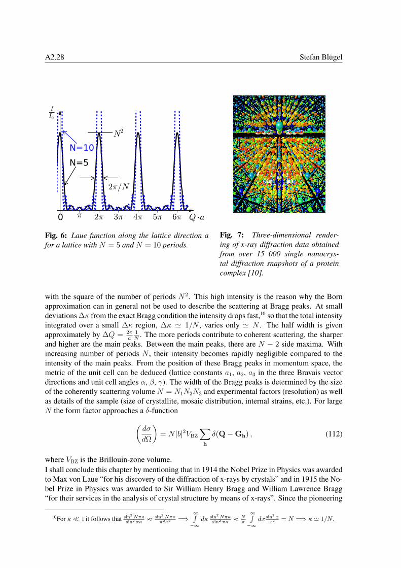
A2.28 Stefan Blugel

Fig. 6: Laue function along the lattice direction afor a lattice with N = 5 and N = 10 periods.

Fig. 7: Three-dimensional render-ing of x-ray diffraction data obtainedfrom over 15 000 single nanocrys-tal diffraction snapshots of a proteincomplex [10].

with the square of the number of periods N2. This high intensity is the reason why the Bornapproximation can in general not be used to describe the scattering at Bragg peaks. At smalldeviations ∆κ from the exact Bragg condition the intensity drops fast,10 so that the total intensityintegrated over a small ∆κ region, ∆κ ' 1/N , varies only ' N . The half width is givenapproximately by ∆Q = 2π

a1N

. The more periods contribute to coherent scattering, the sharperand higher are the main peaks. Between the main peaks, there are N − 2 side maxima. Withincreasing number of periods N , their intensity becomes rapidly negligible compared to theintensity of the main peaks. From the position of these Bragg peaks in momentum space, themetric of the unit cell can be deduced (lattice constants a1, a2, a3 in the three Bravais vectordirections and unit cell angles α, β, γ). The width of the Bragg peaks is determined by the sizeof the coherently scattering volume N = N1N2N3 and experimental factors (resolution) as wellas details of the sample (size of crystallite, mosaic distribution, internal strains, etc.). For largeN the form factor approaches a δ-function(

dσ

dΩ

)= N |b|2VBZ

∑h

δ(Q−Gh) , (112)

where VBZ is the Brillouin-zone volume.I shall conclude this chapter by mentioning that in 1914 the Nobel Prize in Physics was awardedto Max von Laue “for his discovery of the diffraction of x-rays by crystals” and in 1915 the No-bel Prize in Physics was awarded to Sir William Henry Bragg and William Lawrence Bragg“for their services in the analysis of crystal structure by means of x-rays”. Since the pioneering

10For κ 1 it follows that sin2Nπκsin2 πκ

≈ sin2Nπκπ2κ2 =⇒

∞∫−∞

dκ sin2Nπκsin2 πκ

≈ Nπ

∞∫−∞

dx sin2 xx2 = N =⇒ κ ' 1/N .


days of von Laue, Ewald, Knipping, Friedrich, the Bragg’s, Compton, etc., diffraction experi-ments went a long way deciphering today the atomic arrangement of noncrystalline solids suchas viruses as shown in a recent experiment [10] carried out at the Linac Coherent Light Source(LCLS), at SLAC National Accelerator Laboratory in California, USA) as shown in the diffrac-tion image Fig. 7. Physical principles established 100 years ago and subsequent theoretical andexperimental methods developed, reinvented and constantly brought to perfection contribute today and will contribute in the future to the welfare of mankind.

AcknowledgementsI thank Dr. Phivos Mavropoulos and Prof. Peter Dederichs for discussions and Benedikt Schwe-flinghaus for his assistance in preparing the figures.

References[1] J.J. Sakurai, Modern Quantum Theory, (Addison Wesley, 1984).

[2] Wu and Ohmura, Quantum Theory of Scattering, (Prentice Hall, 1962).

[3] A. S. Davidov, Quantum Mechanics, (Pergamon Press, 1991)

[4] N. W. Ashcroft and N. D. Mermin, Solid State Physics, (Brooks Cole, 1976)

[5] Chr. Huygens, Trait de la Lumiere (completed in 1678, published in Leyden in 1690)

[6] Sabrina Disch, Erik Wetterskog, Raphael P. Hermann, German Salazar-Alvarez, PeterBusch, Thomas Bruckel, Lennart Bergstrom, and Saeed Kamali, Nano Lett. 11, 1651(2011).

[7] G. L. Squires, Introduction to the theory of thermal neutron scattering, (Cambridge: Cam-bridge University Press, 1978); (New York: Dover Publications, 1996).

[8] E. Fermi, Ric. Sci. 7, 13 (1936).

[9] E. Fermi, and L. Marshall, Phys. Rev. 71, 666 (1947); Phys. Rev. 72, 408 (1947).

[10] Henry N. Chapman et al., Nature 470, 73 (2011).

scattering theory: born series - forschungszentrum...

Documents