scattering processes in atomic physics, nuclear
TRANSCRIPT
SCATTERING PROCESSESIN ATOMIC PHYSICS, NUCLEAR PHYSICS, AND COSMOLOGY
By
Gavriil Shchedrin
A DISSERTATION
Submitted toMichigan State University
in partial fulfillment of the requirementsfor the degree of
PHYSICS - DOCTOR OF PHILOSOPHY
2013

ABSTRACT
SCATTERING PROCESSESIN ATOMIC PHYSICS, NUCLEAR PHYSICS, AND COSMOLOGY
By
Gavriil Shchedrin
The universal way to probe a physical system is to scatter a particle or radiation off the
system. The results of the scattering are governed by the interaction Hamiltonian of the
physical system and scattered probe. An object of the investigation can be a hydrogen atom
immersed in a laser field, heavy nucleus exposed to a flux of neutrons, or space-time metric
perturbed by the stress-energy tensor of neutrino flux in the early Universe. This universality
of scattering process designates the Scattering Matrix, defined as the unitary matrix of the
overlapping in and out collision states, as the central tool in theoretical physics.
In this Thesis we present our results in atomic physics, nuclear physics, and cosmology. In
these branches of theoretical physics the key element that unifies all of them is the scattering
matrix. Additionally, within the scope of Thesis we present underlying ideas responsible for
the unification of various physical systems. Within atomic physics problems, namely the
axial anomaly contribution to parity nonconservation in atoms, and two-photon resonant
transition in a hydrogen atom, it was the scattering matrix which led to the Landau-Yang
theorem, playing the central role in these problems. In scattering problems of cosmology and
quantum optics we developed and implemented mathematical tools that allowed us to get a
new point of view on the subject. Finally, in nuclear physics we were able to take advantage
of the target complexity in the process of neutron scattering which led to the formulation of
a new resonance width distribution for an open quantum system.

Copyright byGAVRIIL SHCHEDRIN2013
ACKNOWLEDGMENTS
In this section I would like to give a credit to many physicists and mathematicians who
shared their knowledge and shaped my understanding of this beautifully designed Physical
and Mathematical World whose elegance can be appreciated by mere mortals.
The first in the list is my Thesis advisor, Prof. Vladimir G. Zelevinsky, whose knowledge
and real understanding of theoretical physics and in particular nuclear physics is truly
remarkable. My advisor expertise in atomic physics, nuclear physics and cosmology made
possible the very existence of the present Thesis. Also his teaching talent is of the same
caliber as his physics expertise. Here I would like to mention that MSU Physics & Astronomy
Outstanding Faculty Teaching Award of 2003, 2004, and in the unprecedented period of 6
consecutive years from 2006 till 2011 was given to my advisor. So I am very much privileged
and grateful to my great advisor for his willingness to work with such a troublemaker and
crazy guy like me. Most importantly for me, besides physics of course, was his company
where we shared a great deal of fun.
I am very thankful to the Condensed Matter group at Michigan State. First of all, I am
thankful to great physicist Prof. Mark Dykman for his active position in every respect and his
teaching style. The very special thank you goes to Prof. Norman Birge, remarkable physicist
and great experimentalist. His way of explaining physics was absolutely new experience for
me. It was a refreshing point of view on the subject which gave me a practical understanding.
Prof. Thomas Kaplan is the great soul of the condensed matter body at Michigan State.
Prof. Chih-Wei Lai and Prof. John McGuire were very kind to share their time and ideas
with me.
iv

I am grateful to the High Energy group at Michigan State. I am thankful to Prof.
Wayne Repko for an exciting problem in cosmology and for the reference to a jewel in the
modern physics literature, a masterpiece by the greatest living physicist Steven Weinberg,
named Cosmology, published by the Oxford University Press in 2008. If someone wants to
appreciate a truth beauty of the Physical World, this book will blow someone’s mind as it
happened with me while I was writing this Thesis. I would like to thank Prof. Carl Schmidt
for his courses on Quantum Field Theory and Mathematical Physics. Also I would like to
thank Prof. James Linnemann, Prof. Carl Bromberg and Prof. Kirsten Tollefson, supported
by the team of Tibor Nagy, Richard Hallstein and Mark Olson, who guided me thorough my
teaching courses at Michigan State. On the top of that, Prof. James Linnemann has always
been a great audience to discuss theoretical physics.
The physics division where I finally settled down had become Nuclear Cyclotron facility
at Michigan State. Prof. Scott Pratt who is the Graduate Program Director and who was
a witness of my ups and downs during my four years long graduate life, has always been
a great audience to discuss physics in a “five minutes” format. I would like to thank Prof.
Alex Brown and Prof. Remco Zegers for their time and efforts during my nuclear graduate
life. I am thankful to Prof. Michael Thoennessen whose invisible help has always been very
much appreciated.
Mathematics department at Michigan State has a number of great mathematicians. I
am very thankful to great mathematician Prof. Alexander Volberg for his keen interest in
physics that resulted in our joint paper. The chapter on quantum optics in this Thesis is
based on our work. Also I am indebted to a wonderful mathematician Prof. Michael Shapiro,
who shared his time and mathematical insights on the mathematical structures appearing
in nuclear physics problems.
v
From my undergraduate life in St. Petersburg I would like to thank remarkable physicist
Prof. Alexander N. Vasil’ev for his rich contribution to my undergraduate physics life which
would have been completely empty otherwise. Also I am grateful to my undergraduate
advisor, great physicist Prof. Leonti N. Labzowsky, who shared quite a bit of his time
and knowledge with me. Most importantly, he shared a very interesting problem on axial
anomaly that grew into a single chapter on atomic physics in this Thesis.
The present list would never be a complete one without paying a tribute to a truly
remarkable people, Anna G. Reznikova, Sergey G. Maloshevsky, and Inna D. Mints, all
wonderful mathematicians, who helped me get started and supported me wholeheartedly
during my rough undergraduate years in St. Petersburg.
Finally I would like to thank all of my fellow physics graduate students at Michigan
State, and in particular Pawin Ittisamai and Scott Bustabad who shared a great deal of
humor during my graduate life. Also I am grateful to my undergraduate students who
suffered at my physics classes and from whom I have learned quite a bit.
Thank all of you!
vi

TABLE OF CONTENTS
LIST OF FIGURES . . . . . . . . . . . . . . . . . . . . . . . . . . . . . . . . . . . ix
Chapter 1 Introduction . . . . . . . . . . . . . . . . . . . . . . . . . . . . . . . 1
Chapter 2 Atomic Physics . . . . . . . . . . . . . . . . . . . . . . . . . . . . . . 42.1 Standard Model in low-energy physics . . . . . . . . . . . . . . . . . . 52.2 Furry theorem . . . . . . . . . . . . . . . . . . . . . . . . . . . . . . . . . 62.3 Axial Anomaly . . . . . . . . . . . . . . . . . . . . . . . . . . . . . . . . . 82.4 Axial Anomaly S-matrix . . . . . . . . . . . . . . . . . . . . . . . . . . . 102.5 Z-boson decay . . . . . . . . . . . . . . . . . . . . . . . . . . . . . . . . . 142.6 PNC amplitude . . . . . . . . . . . . . . . . . . . . . . . . . . . . . . . . . 21
Chapter 3 Quantum Optics . . . . . . . . . . . . . . . . . . . . . . . . . . . . . 323.1 Introduction . . . . . . . . . . . . . . . . . . . . . . . . . . . . . . . . . . . 323.2 Laser-assisted hydrogen recombination . . . . . . . . . . . . . . . . . . 333.3 S-matrix . . . . . . . . . . . . . . . . . . . . . . . . . . . . . . . . . . . . . 343.4 The Coulomb-Volkov wave function . . . . . . . . . . . . . . . . . . . . 373.5 The partial cross section . . . . . . . . . . . . . . . . . . . . . . . . . . . 383.6 The summation procedure and cross section . . . . . . . . . . . . . . . 393.7 The soft photon approximation . . . . . . . . . . . . . . . . . . . . . . . 423.8 Summary . . . . . . . . . . . . . . . . . . . . . . . . . . . . . . . . . . . . . 43
Chapter 4 Nuclear Physics . . . . . . . . . . . . . . . . . . . . . . . . . . . . . 454.1 Introduction . . . . . . . . . . . . . . . . . . . . . . . . . . . . . . . . . . . 464.2 Resonance width distribution . . . . . . . . . . . . . . . . . . . . . . . . 494.3 Effective non-Hermitian Hamiltonian and scattering matrix . . . . . 524.4 From ensemble distribution to single width distribution . . . . . . . 544.5 Doorway approach . . . . . . . . . . . . . . . . . . . . . . . . . . . . . . . 574.6 Photon emission channels . . . . . . . . . . . . . . . . . . . . . . . . . . 604.7 Many-channel case . . . . . . . . . . . . . . . . . . . . . . . . . . . . . . . 644.8 Conclusion . . . . . . . . . . . . . . . . . . . . . . . . . . . . . . . . . . . . 67
Chapter 5 Cosmology . . . . . . . . . . . . . . . . . . . . . . . . . . . . . . . . 695.1 Introduction . . . . . . . . . . . . . . . . . . . . . . . . . . . . . . . . . . . 695.2 Fluctuations in General Relativity . . . . . . . . . . . . . . . . . . . . . 715.3 Boltzmann equation for neutrinos . . . . . . . . . . . . . . . . . . . . . 775.4 Momentum representation . . . . . . . . . . . . . . . . . . . . . . . . . . 825.5 Perturbations to the energy-momentum tensor . . . . . . . . . . . . . 85
vii

5.6 Gravitational wave damping . . . . . . . . . . . . . . . . . . . . . . . . . 895.7 Matter-radiation equality . . . . . . . . . . . . . . . . . . . . . . . . . . 925.8 Late-time evolution of the gravitational wave damping . . . . . . . . 965.9 Early-time evolution of the gravitational wave damping . . . . . . . 1025.10 General solution for the gravitational wave damping . . . . . . . . . 1085.11 Evaluation of the convolution integrals . . . . . . . . . . . . . . . . . . 1135.12 Conclusion . . . . . . . . . . . . . . . . . . . . . . . . . . . . . . . . . . . . 117
Chapter 6 Conclusions . . . . . . . . . . . . . . . . . . . . . . . . . . . . . . . . 119
APPENDICES . . . . . . . . . . . . . . . . . . . . . . . . . . . . . . . . . 124A Electron wave function behavior near the nucleus . . . . . . . . . . . 124B Secular equation in the general case . . . . . . . . . . . . . . . . . . . . 125C Friedmann equations . . . . . . . . . . . . . . . . . . . . . . . . . . . . . 126D Energy density for fermions and bosons in the early Universe . . . 129E Convolution integral of spherical Bessel functions . . . . . . . . . . . 133F Convolution matrices in the late-time limit . . . . . . . . . . . . . . . 137G Convolution matrix in the early-time limit . . . . . . . . . . . . . . . . 139H Convolution matrices in the early-time limit . . . . . . . . . . . . . . 140
BIBLIOGRAPHY . . . . . . . . . . . . . . . . . . . . . . . . . . . . . . 143
viii

LIST OF FIGURES
Figure 2.1 Proof of the Furry theorem on the example of a triangle Feynmangraph. . . . . . . . . . . . . . . . . . . . . . . . . . . . . . . . . . . 7
Figure 2.2 The Feynman graphs that describe PNC effect in cesium. The doublesolid line denotes the electron in the field of the nucleus. The wavyline denotes the photon (real or virtual) and the dashed horizontal linewith the short thick solid line at the end denotes the effective weakpotential, i.e. the exchange by Z-boson between the atomic electronand the nucleus. Graph (a) corresponds to the basic M1 transitionamplitude, graph (b) corresponds to the E1 transition amplitude,induced by the effective weak potential. The latter violates the spatialparity and allows for the arrival of p-states in the electron propagatorin graph (b), of which the contributions of 6p and 7p states dominate.The standard PNC effect arises due to the interference betweengraphs (a) and (b). Graph (c) corresponds to the axial anomaly.The thin solid lines represent virtual electrons and positrons. Tograph (c), the Feynman diagram with interchanged external photonand Z-boson lines should be added. . . . . . . . . . . . . . . . . . . 9
Figure 2.3 Flow of momenta in the axial anomaly. . . . . . . . . . . . . . . . . 12
Figure 2.4 Feynman diagram of Z-boson decay into two photons. . . . . . . . 15
Figure 2.5 Feynman diagram of π0-meson decay into two photons. . . . . . . . 16
Figure 4.1 The proposed resonance width distribution according to eq. (4.3)with a single neutron channel in the practically important case η Γ.The width Γ and mean level spacing D are measured in units of themean value 〈Γ〉. “For interpretation of the references to color in thisand all other figures, the reader is referred to the electronic versionof this dissertation.” . . . . . . . . . . . . . . . . . . . . . . . . . . . 50
Figure 4.2 The proposed resonance width distribution according to eq. (4.28)with a single neutron channel and N gamma-channels in thepractically important case η Γ. The neutron width Γ, radiationwidth γ, and mean level spacing D are measured in units of the meanvalue 〈Γ〉. . . . . . . . . . . . . . . . . . . . . . . . . . . . . . . . . . 62
ix
Figure 5.1 Graphical representation for the upper but one triangular structureof the matrix B2k,2l, eq. (70). The matrix indices l and k define aposition of the matrix element in the xy-plane, while along z-axis weplot its value. . . . . . . . . . . . . . . . . . . . . . . . . . . . . . . 98
Figure 5.2 Late-time evolution of the gravitational wave damping D(u) in theearly Universe. . . . . . . . . . . . . . . . . . . . . . . . . . . . . . . 100
Figure 5.3 Graphical representation for the upper triangular structure of thematrix F2k,2l, eq. (72). The matrix indices l and k define the positionof the matrix element in the xy-plane, while along z-axe we plot itsvalue. . . . . . . . . . . . . . . . . . . . . . . . . . . . . . . . . . . . 104
Figure 5.4 Damping of gravitational wave as a function of conformal time u inthe early-time limit. Solid line corresponds to the exact solution ofthe gravitational wave damping in the early-time limit and dashedline is the approximate solution, A0j0(u), eq. (5.166). . . . . . . . . 106
Figure 1 Graphical representation for the upper but one triangular structureof the matrix B2k,2l. The matrix indices l and k define a position ofthe matrix element in the xy-plane, while along z-axe we plot its value.137
Figure 2 Graphical representation for the upper but one triangular structure ofthe matrix B2k+1,2l+1. The matrix indices l and k define a positionof the matrix element in the xy-plane, while along z-axe we plot itsvalue. . . . . . . . . . . . . . . . . . . . . . . . . . . . . . . . . . . . 138
Figure 3 Graphical representation for the upper triangular structure of thematrix F2k,2l, eq. (72). The matrix indices l and k define the positionof the matrix element in the xy-plane, while along z-axe we plot itsvalue. . . . . . . . . . . . . . . . . . . . . . . . . . . . . . . . . . . . 139
Figure 4 Graphical representation for the upper triangular structure of thematrix A2k+1,2l. The matrix indices l and k define the position ofthe matrix element in the xy-plane, while along z-axe we plot its value.140
Figure 5 Graphical representation for the upper triangular structure of thematrix A2k,2l+1. The matrix indices l and k define the position ofthe matrix element in the xy-plane, while along z-axe we plot its value.141
x
Chapter 1
Introduction
In this Thesis we summarize our results in atomic physics, quantum optics, nuclear physics,
and cosmology unified by various aspects of quantum scattering theory.
In Chapter 2 our object of investigation is the scattering matrix corresponding to the
axial anomaly contribution to parity nonconservation in atoms. Here we explain physics of
parity nonconservation in complex atoms and discuss the contribution of the axial anomaly to
parity nonconservation in atomic cesium. The main result is the prediction of the emission of
an electric photon by the magnetic dipole which has not been observed yet. The probability
of this process is very small but the non-zero result is important from theoretical point of
view.
The main aspect of our calculation is related to the well known theorem of axial anomaly
cancellation in the Standard Model. According to the Landau-Yang theorem, it is impossible
for the real Z-boson of spin J = 1 to decay into two real photons in contrast to the allowed
two-photon decay of the spinless π0-meson. However, if one of the photons that connects
the triangular graph of the axial anomaly with the electron atomic transition, e.g., 6s − 7s
transition in cesium, is virtual, the axial anomaly does not vanish. We have shown that one
can see the impact of the axial anomaly in atomic physics through the parity violation in
atoms.
1
Chapter 3 is devoted to the electron scattering process off an arbitrary central potential
in the presence of strong laser field. Here we introduce a new method that allows one to
obtain an analytical cross section for the laser-assisted electron-ion collision. As an example
we perform a calculation for the hydrogen laser-assisted recombination. The standard S-
matrix formalism is used for describing the collision process. The S-matrix is constructed
from the electron Coulomb-Volkov wave function in the combined Coulomb-laser field and
the hydrogen perturbed state. By the aid of the Bessel generating function, the S-matrix
is decomposed into an infinite series of the field harmonics. We have introduced a new step
that results in an analytical expression for the cross section of the process. The theoretical
novelty is in the application of the Plancherel theorem to the Bessel generating function.
This allows one to perform summation of the infinite series of Bessel functions and thus
obtain a closed analytical expression for the laser-assisted hydrogen photo-recombination
process.
In the field of nuclear physics presented in Chapter 4 we investigate the resonance width
distribution for low-energy neutron scattering off heavy nuclei. Our interest was ignited by
the recent experiments that claimed significant deviations from the routinely used chi square,
or the Porter-Thomas, distribution. The unstable complex nucleus is an open quantum
system, where the intrinsic dynamics has to be supplemented by the coupling of chaotic
internal states through the continuum. We propose a new width distribution based on
random matrix theory for a chaotic quantum system with a single decay channel as well
as for an open quantum system with an arbitrary number of open channels. The revealed
statistics of the width distribution exhibits distinctive properties that are characteristically
different from the regularities shared by closed quantum systems.
2

In Chapter 5 our object of investigation is the space-time metric perturbed by the stress-
energy tensor of neutrino scattering in the early Universe. In this Chapter we have developed
a mathematical machinery that allows one to evaluate gravitational wave damping due to
freely streaming neutrinos in the early Universe. The solution is represented by a convergent
series of spherical Bessel functions derived with the help of a new compact formula for
the convolution of spherical Bessel functions of integer order. These calculations can be
compared to the tensor fluctuations of the Cosmic Microwave Background in order to reveal
direct evidence of the presence of gravitational waves in the early Universe. The developed
technique can be applied for the analysis of the scalar Cosmic Microwave Background
fluctuations which provides a direct test of the standard inflationary cosmological model.
Finally, Chapter 6 summarizes the results of our investigation on scattering processes in
atomic physics, quantum optics, nuclear physics, and cosmology. Basic governing principles,
such as conservation laws and detailed balance principle, unitarity and gauge invariance of
the scattering matrix are given special attention throughout the Thesis.
3
Chapter 2
Atomic Physics
In this chapter the main interest is parity violation in atomic physics. Parity operation
is defined as a coordinate inversion ~r → −~r, which tests the coordinate symmetry of the
physical system, as well as intrinsic symmetries of fundamental physical objects. In quantum
electrodynamics (QED) that fully describes electron-photon interaction, parity is conserved
due to the invariance of the QED action under the spatial inversion.
However, in the Standard Model that treats electromagnetic and weak forces as a unified
electroweak interaction, which led to a prediction and subsequent discovery of the W and Z
bosons, parity is violated. The W and Z bosons are the carriers of the so-called weak axial
currents which are responsible for the parity violation.
In addition to the high energy experiments, that aim at the verification of the Standard
Model on a very high energy scale, one can test its predictions on a low energy scale by
running tabletop experiments. In particular, we are interested in parity non-conservation
effects in atoms, driven by the effective parity nonconserving interaction of electrons with
the nucleus.
This chapter is organized as follows. In the first subsection we briefly review the general
scope of the problem. In the section on the Furry theorem we provide an important result
for the fermion loop diagrams with an odd number of interaction vertices, e.g. one on Fig.
2.1. Next subsection stands for a general physical idea behind axial anomaly calculation in
atomic physics. The actual calculation is presented in section Axial Anomaly S-matrix. In
4

this section we explicitly write the S-matrix for the decay of the Z-boson into two photons
and apply it to our calculation. We show that due to the transversality conditions and
on-shell constraint for real photons and the Z-boson, the axial anomaly diagram identically
vanishes, in a full accordance with the Landau-Yang theorem. However, if one of the photons
that connects the triangular graph of the axial anomaly with the electron atomic transition,
e.g., 6s−7s transition in cesium, is virtual, the axial anomaly does not vanish and contributes
to the effect of parity nonconservation.
The results of this chapter are based on our paper,
GS and L. Labzowsky, Phys. Rev. A 80, 032517 (2009).
2.1 Standard Model in low-energy physics
The problem of testing the Standard Model (SM) in the low-energy physical phenomena is
one of the interesting topics in physics actively pursued in the last few decades. The SM
in the low energy limit is tested in nuclei, where significant many-body enhancement of the
parity nonconservation (PNC) effects was predicted and confirmed. Along with the PNC
effects in nuclei, atomic physics experiments offer a high precision for validating the SM
predictions. The most accurate of atomic experiments is the one with the neutral cesium
atom, first proposed in [1] and performed with the utmost precision in [2].
The basic atomic transition employed in the cesium experiment was the strongly
forbidden 6s − 7s transition of the valence electron with the absorption of a magnetic
dipole photon, M1. In the real experiment this very weak transition was opened by the
external electric field but it does not matter for our further derivations. The Feynman
5

graphs illustrating the PNC effect in cesium are given below in Fig. 2.2.
The atomic experiments are indirect and require very accurate calculations of the PNC
effects to extract the value of the characteristic parameter of the SM, the Weinberg angle,
which can be compared with the corresponding high-energy value. The main difficulty with
the PNC calculations in neutral atoms is the necessity to take into account the electron
correlations within the complex atom. Therefore the experiments with much simpler systems,
such as few-electron highly charged ions (HCI) would be highly desirable. Several proposals
on the subject were considered in [3–6]. At the same time relativistic corrections make
heavy-Z atoms preferable due the enhancement factor for electronic wave functions.
The radiative corrections to the PNC effect are important in cesium calculations to reach
the agreement with the high-energy SM predictions. These radiative corrections include
electron self-energy, vertex and vacuum polarization Feynman diagrams. They are even
more important in the case of the HCI. The entire set of these corrections for the neutral
cesium atom was calculated in [7–10]. The electron self-energy and vertex corrections for
HCI were obtained in [11]; the vacuum polarization correction was given in [12].
The full set of radiative corrections including Z-boson loops has not been calculated,
neither for a neutral atom nor for the HCI. Therefore the problem still cannot be considered
as fully solved.
2.2 Furry theorem
In quantum field theory Feynman diagrams with a high number of vertices are notoriously
difficult for calculation. However, in the special case of a fermion loop diagram with an odd
number of identical interaction vertices, its contribution, according to the Furry theorem,
6

γ
γ
γ
γµ
γν
γλ
p
k1
k2
p− k2
p+ k1
q
Figure 2.1: Proof of the Furry theorem on the example of a triangle Feynman graph.
is identically zero. To illustrate the proof of the Furry theorem we recognize that the Dirac
matrices γµ change sign and get transposed, γµ, under charge conjugation C,
C−1γµC = −γµ, (2.1)
while the charge conjugated fermion propagator modifies according to
C−1G(p)C = C−1[pνγ
ν +me
p2 −m2e
]C =
[−pν γν +me
p2 −m2e
]= G(−p). (2.2)
Therefore a typical triangle amplitude will change sign under charge conjugation,
7

Aµνλ(k1, k2) = (2.3)∫d4p Tr
[γµ6 p +me
p2 −m2eγν6 p− 6 k2 +me
(p− k2)2 −m2eγλ6 p+ 6 k1 +me
(p+ k1)2 −m2e
]−→ (−1)3
∫d4p Tr
[γµ6 p +me
p2 −m2eγν6 p− 6 k2 +me
(p− k2)2 −m2eγλ6 p+ 6 k1 +me
(p+ k1)2 −m2e
]≡ 0.
The same argument holds for a Feynman diagram with an arbitrary number of odd fermion-
boson vertices, and we thus prove the Furry theorem.
However, if a Feynman diagram has an odd number of vertices of a different kind, for
instance, two vector photon vertices, and a single π0 pseudo-scalar vertex, or a single Z-boson
pseudo-vector vertex, the corresponding Feynman diagram has a non-zero value.
2.3 Axial Anomaly
In the present work we consider a very special radiative correction to the PNC effect,
presented by a triangular Feynman graph, or axial anomaly (AA). We understand the triangle
AA as a fermion loop with at least one weak vertex [13]. Our conclusion will be that in a
neutral atom the contribution of the axial anomaly is non-zero albeit relatively small.
The leading contribution of the AA to the atomic PNC effect is depicted in Fig. 2.2 (c).
This contribution corresponds to the Adler-Bell-Jackiw anomaly [14]. In this work we will
concentrate exclusively on this term.
The final answer, that looks like the emission of the electric photon by the magnetic
dipole, can be easily understood before any real calculations are made. Suppose we have the
6s-7s transition in cesium. The virtual photon in this transition that connects the atomic
electron line with the triangular graph of the axial anomaly must be of a magnetic dipole
type M1. This virtual photon is absorbed by the fermion current in the axial anomaly
8

a
M1
7s
6s
7s
6s
Z
E1
6p, 7p
7s
6s
Z
b c
E1
Figure 2.2: The Feynman graphs that describe PNC effect in cesium. The double solid linedenotes the electron in the field of the nucleus. The wavy line denotes the photon (real orvirtual) and the dashed horizontal line with the short thick solid line at the end denotes theeffective weak potential, i.e. the exchange by Z-boson between the atomic electron and thenucleus. Graph (a) corresponds to the basic M1 transition amplitude, graph (b) correspondsto the E1 transition amplitude, induced by the effective weak potential. The latter violatesthe spatial parity and allows for the arrival of p-states in the electron propagator in graph(b), of which the contributions of 6p and 7p states dominate. The standard PNC effectarises due to the interference between graphs (a) and (b). Graph (c) corresponds to theaxial anomaly. The thin solid lines represent virtual electrons and positrons. To graph (c),the Feynman diagram with interchanged external photon and Z-boson lines should be added.
9

triangle, through a first vertex, and cannot change the parity of the fermion current flowing
through this vertex. Now, the second vertex in the axial anomaly triangle that is responsible
for exchange of the Z-boson between the fermion line and the cesium nucleus has the Dirac
matrix γ5 that changes the parity of the fermion line. As the result, the third vertex in the
axial anomaly triangle that connects two fermion lines with an opposite parity must emit
the electric photon type E1.
2.4 Axial Anomaly S-matrix
We employ the standard expression for the effective parity nonconserving interaction of the
atomic electron with the nucleus [15] in the form
HW = APNCρ0(~r)γ5, (2.4)
with parity nonconservation vertex APNC,
APNC = −GFQW2√
2, (2.5)
Dirac pseudoscalar matrix γ5,
γ5 = iγ0γ1γ2γ3 = − i
4!εµνρσγ
µγνγργσ =
0 1
1 0
, (2.6)
and contact electron-nucleus interaction ρ0(~r), where one can neglect the finite size of an
atomic nucleus,
ρ0(~r) = δ(~r). (2.7)
10

GF is the Fermi constant given in terms of the proton mass mp by
GF = 1.027× 10⁻⁵ 1
m2p
= 1.166× 10⁻⁵ 1
GeV2. (2.8)
QW is the weak charge of the nucleus,
QW = −N + Z(1− 4 sin2 θw), (2.9)
while Z and N are the numbers of protons and neutrons in the nucleus, and θw is the
Weinberg angle. The currently accepted value for this parameter is
sin2 θw ' 0.23. (2.10)
The singular δ-function potential acting in the space of Dirac electron wave functions does
not vanish only when electron and nucleon coordinates coincide. This approximation is valid
if the transferred momentum q is much less than the mass of Z-boson, which is clearly valid
for the atomic electron. For the electron in the loop this approximation is valid due to the
fact that the momentum transfer to the nucleus, as one can see on Fig. 2.3, is (q − k)
where q2 m2Z , and as the consequence (q− k)2 m2
Z . Therefore we can parametrize the
coupling of the electron-nucleon interaction by the contact interaction (2.4).
11

p′1
p1
qp
p + q
k
p + k
q − k
γν
γµ
γλγ5
γρ
Figure 2.3: Flow of momenta in the axial anomaly.
We write down the S-matrix corresponding to the amplitude Fig. 2.2 (c) in the
momentum representation (see Fig. 2.3):
S = (ie)3∫
d4p′1(2π)4
d4p1
(2π)4
d4p
(2π)4Ψn′s(p1)γρΨns(p
′1)
gρν
q2 + iε(2.11)
×Tr
[γµ6 p+me
p2 −m2eγν6 p+ 6 q +me
(p+ q)2 −m2eγλγ5 6 p+ 6 k +me
(p+ k)2 −m2e
]V PNCλ (q − k)Aµ(k).
12

Here e and me are the electron charge and mass,
Ψns(p) = Ψns(~p)δ(p0 − εns) (2.12)
is the wave function of the bound atomic electron in the state |ns〉 with εns being the energy
of this state, the transferred momentum q is
q = p1 − p′1, (2.13)
gρν is the pseudo-Euclidean metric tensor,
gρν =
1 0 0 0
0 −1 0 0
0 0 −1 0
0 0 0 −1
, (2.14)
γµ are the Dirac matrices,
γµ =
0 σµ
−σµ 0
≡ 0 σ
−σ 0
, (2.15)
γ0 ≡ β =
1 0
0 -1
, (2.16)
and Aµ(k) is the wave function of the emitted photon,
Aµ(x) =
√2π
ωεµe−ikx, (2.17)
13

in the momentum representation. Here εµ and k = (ω,k) are the four-vectors of the
polarization and the momentum of the emitted photon, correspondingly.
In the momentum representation the potential V PNCλ for the parity-nonconserving
interaction of the electron with the nucleus is
V PNCλ (q − k) = APNCρ0(q − k)δλ0, (2.18)
where the nucleon density in the particular case of the point-like nucleus is
ρ0(q − k) = 2πδ(q0 − k0). (2.19)
In this chapter we use the relativistic units with h = c = 1.
2.5 Z-boson decay
The central element in the Feynman diagram of Fig. 2.3, the fermion triangle, involves
two photon vertices and a single Z-boson vertex. First we consider the Z-boson (with spin
J(Z) = 1) decay [16] into two photons, Fig. 2.4. The Landau theorem forbids this decay
because a two-photon system cannot exist with angular momentum J = 1 [17,18], in contrast
to the allowed decay π0 → γγ since J(π0) = 0 [19], see Fig. 2.5. We shall derive this result
in the Feynman diagram language for the S-matrix of Fig. 2.4, and see implications for the
diagram in Fig. 2.3.
The S-matrix of the Z-boson decay into two photons, Fig. 2.4, is proportional to
Sµνλ(k1, k2) =
∫d4p Tr
[γµ6 p +me
p2 −m2eγν6 p− 6 k2 +me
(p− k2)2 −m2eγλγ5 6 p+ 6 k1 +me
(p+ k1)2 −m2e
]. (2.20)
14

Z
γ
γ
γµ
γν
γλγ5
p
k1
k2
p− k2
p+ k1
q
Figure 2.4: Feynman diagram of Z-boson decay into two photons.
A simple change of variables in the Z-boson amplitude (2.20),
k1 → k, (2.21)
k2 → −q,
leads to the loop integral in the original PNC-amplitude, eq. (2.11).
Here we shall note that the trace of a product of the Dirac γ5 matrix with the four other
distinct Dirac matrices leads to a non-vanishing result,
Tr[γ5γτγµγνγλ
]= 4iετµνλ, (2.22)
15
π0
γ
γ
γµ
γν
γ5
p
k1
k2
p− k2
p+ k1
q
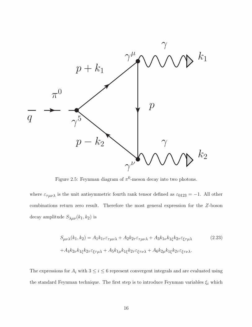
Figure 2.5: Feynman diagram of π0-meson decay into two photons.
where ετµνλ is the unit antisymmetric fourth rank tensor defined as ε0123 = −1. All other
combinations return zero result. Therefore the most general expression for the Z-boson
decay amplitude Sλµν(k1, k2) is
Sµνλ(k1, k2) = A1k1τετµνλ + A2k2τετµνλ + A3k1νk1ξk2τεξτµλ (2.23)
+A4k2νk1ξk2τεξτµλ + A5k1µk1ξk2τεξτνλ + A6k2µk1ξk2τεξτνλ.
The expressions for Ai with 3 ≤ i ≤ 6 represent convergent integrals and are evaluated using
the standard Feynman technique. The first step is to introduce Feynman variables ξi which
16

simplify the loop integral (2.20),
1
α1α2α3= 2!
∫ 1
0dξ1
∫ 1
0dξ2
∫ 1
0dξ3
δ(1− ξ1 − ξ2 − ξ3)
(α1ξ1 + α2ξ2 + α3ξ3)3(2.24)
≡ 2!
∫ 1
0dξ1
∫ ξ1
0dξ2
1
(α1ξ2 + α2(ξ1 − ξ2) + α3(1− ξ1))3.
In our specific case the variables αi are
α1 = (p+ k1 + k2)2 −m2e, (2.25)
α2 = (p+ k2)2 −m2e, (2.26)
α3 = p2 −m2e. (2.27)
Therefore the loop integral becomes
1
α1α2α3≡ 1
[(p+ k1 + k2)2 −m2e][(p+ k2)2 −m2
e][p2 −m2
e](2.28)
= 2!
∫ 1
0dξ1
∫ ξ1
0dξ2
1
(α1ξ2 + α2(ξ1 − ξ2) + α3(1− ξ1))3.
First we shall simplify the denominator in eq. (2.28) as follows:
[(p+ k1 + k2)2 −m2e]ξ2 + [(p+ k2)2 −m2
e](ξ1 − ξ2) + [p2 −m2e](1− ξ1)
= p2 − 2p(−k2ξ1 − k1ξ2) + (−m2 + 2k2k1ξ2 + k21ξ2 + k2
2ξ1). (2.29)
17

Further we notice a common integral
∫d4p
(p2 + l − 2pk)3=
iπ2
2(l − k2), (2.30)
and the loop integral becomes
∫d4p
1
[(p+ k1 + k2)2 −m2e][(p+ k2)2 −m2
e][p2 −m2
e](2.31)
= 2!
(iπ2
2
)∫ 1
0dξ1
∫ ξ1
0dξ2
1
−m2 + 2k2k1ξ2 + k21ξ2 + k2
2ξ1 − (k2ξ1 + k1ξ2)2.
Finally the expression of eq. (2.31) can be simplified by the change of variable
ξ1 −→ 1− ξ1, (2.32)
and the denominator in eq. (2.31) becomes
−m2 + 2k2k1ξ2 + k21ξ2 + k2
2(1− ξ1)− (k2(1− ξ1) + k1ξ2)2 (2.33)
= −m2 + k21ξ2 + k2
2ξ1 − (k2ξ1 − k1ξ2)2.
Finally the expressions for Ai with 3 ≤ i ≤ 6 will be expressed in terms of the convergent
integrals
Jrst(k1, k2) =1
π2
∫ 1
0dξ1
∫ 1
0dξ2
∫ 1
0dξ3
(ξ1rξ1
sξ3t)δ(1− ξ1 − ξ2 − ξ3)
(ξ1ξ2(k1 + k2)2 + ξ1ξ3k21 + ξ2ξ3k
22 −m2)
. (2.34)
In order to obtain a convergent and gauge invariant expression for the amplitude Sµνλ we
18

impose the Ward identities,
k1µSµνλ = 0, (2.35)
k2νSµνλ = 0. (2.36)
In terms of the general expression (2.23), eqs. (2.35) and (2.36) lead to the desirable
constraints on the divergent integrals
[−A2 + k21A5 + (k1k2)A6]k1ξk2τεξτνλ = 0, (2.37)
[−A1 + k22A4 + (k1k2)A3]k1ξk2τεξτµλ = 0. (2.38)
In this way the amplitude Sµνλ will be finite and gauge-invariant if we choose A2(k1, k2)
and A1(k1, k2) in the form
A2(k1, k2) = k21A5 + (k1k2)A6, (2.39)
A1(k1, k2) = k22A4 + (k1k2)A3. (2.40)
19

Finally we come to the Z-boson amplitude Sµνλ,
Sµνλ(k1, k2) = J110(k1, k2)εµναβk1αk2β(k1 + k2)λ (2.41)
+J101(k1, k2)(ελναβk1αk2βk1µ + k21ελµναk2α)
+J011(k1, k2)(ελµαβk1αk2βk2ν + k22ελµναk1α),
with the integrals Jrst(k1, k2) given by eq. (2.34).
Due to the transversality conditions for the Z-boson and on-shell photons expressed as
(k1 + k2)λελ = 0,
ε1µk1µ = 0, (2.42)
ε2νk2ν = 0,
and conditions for the real photons,
k21 = 0, (2.43)
k22 = 0,
we arrive at the result of the Landau theorem SZγγ = 0. But in our case one of the photons
(e.g. with index 2) is virtual, as well as the Z-boson. Therefore the initial S-matrix (2.11)
returns a nonzero result.
20

2.6 PNC amplitude
The next step is to contract the Z-boson amplitude Sµνλ with the Z-boson δ-potential,
photon polarization vector, and photon propagator,
Sµνλ(k, q)δλ0ε1µa2ν , (2.44)
where
a2ν =γ0γρgρν
q2=αρgρν
q2=ανq2, (2.45)
with Dirac α-matrices
αµ = γ0γµ =
0 σ
σ 0
. (2.46)
By noticing
ε0µνα = −εµνα, (2.47)
we finally arrive at the axial anomaly amplitude,
Sµνλ(k, q)δλ0ε1µανq2
= J011(k, q)[εµαβkαqαε1µ(α, q) + εµναε1µkααν ]
= J011(k, q)
(ε, [k × q])(α, q)
q2+ (ε, [α×k])
, (2.48)
21

and S-matrix for the PNC effect is
S = (ie)3APNCδ(Ef − Ein − ω0)
√4π
2ω0(2.49)
×∫
d3p′1(2π)3
d3p1
(2π)3Ψ+(p1)J011(k, q)
[(ε, [k × q])(α, q)
q2+ (ε, [α×k])
]Ψ(p′1).
Next we turn our attention to non-relativistic analysis of the S-matrix. The lower component
of the Dirac electron wave function χ is expressed in terms of the upper one ϕ via
χ =(σp)
2mϕ. (2.50)
Dirac α-matrices mix these components,
(ϕ∗1 χ∗1
) 0 σ
σ 0
ϕ
′1
χ′1
, (2.51)
which reduces to
ϕ∗1
[σ
(σp′1)
2m+
(σp1)
2mσ
]ϕ′1. (2.52)
The first term in square brackets in eq. (2.49) can be simplified to
(q, [ε× k])(σ, q)
q2(σp′1) + (σp1)
(q, [ε× k])(σ, q)
q2, (2.53)
while the second term reduces to
(σ, [k×ε])(σp′1) + (σp1)(σ, [k×ε]). (2.54)
22

Further we employ the well-known identity for the Pauli matrices,
(σa)(σb) = (ab) + i(σ, [a× b]), (2.55)
and owing to the transferred momentum is q = p1 − p′1, eq. (2.53) becomes
(q, [ε× k])(σ, q)
q2(σp′1) + (σp1)
(q, [ε× k])(σ, q)
q2= (q, p1 + p′1)
(q, [ε× k])
q2. (2.56)
In order to simplify eq. (2.54) we use the identities
(σ, [k × ε])(σp′1) = ([k × ε], p′1) + i(σ, [[k × ε]× p′1]]), (2.57)
(σp1)(σ, [k × ε]) = (p1, [k × ε]) + i(σ, [p1 × [k × ε]]). (2.58)
Therefore the sum of these terms is
(σ, [k × ε])(σp′1) + (σp1)(σ, [k × ε]) (2.59)
= (p1 + p′1, [k × ε]) + i(σ, [q × [k × ε]])
= (p1 + p′1, [k × ε]) + i(σk)(qε)− i(σε)(qk),
which represents the final expression for eq. (2.54). For the sake of convenience we introduce
P = p1 + p′1, (2.60)
23

and then the square brackets of the S-matrix in eq. (2.49) will be represented as
(q, P )(q, [ε× k])
q2+ (P, [k × ε]) + i(σk)(qε)− i(σε)(qk). (2.61)
Now we have to explore how the obtained expression changes under change of integration
variables
p1 −→ −p1, (2.62)
p′1 −→ −p′1.
The expression in eq. (2.59) changes sign and therefore we shall turn our attention to the
integral (2.34) which simplifies in the case for a real emitted photon k21 = 0,
I(k, q) =1
π2
∫ 1
0dξ1
∫ 1−ξ1
0dξ2
ξ1(ξ1 + ξ2 − 1)
−m2 + 2ξ1ξ2(kq) + ξ1(1− ξ1)q2, (2.63)
and in the non-relativistic limit we obtain
1
m2 − 2ξ1ξ2(kq)=
1
m2
[1 +
2ξ1ξ2(kq)
m2+O
(1
m4
)]. (2.64)
Finally, we have the expression which is even under the inversion (2.62),
(q, P )(q, [ε× k])
q2(qk) + (P, [k × ε])(qk) + i(σk)(qε)(qk)− i(σε)(qk)2. (2.65)
After integration over(p1, p
′1
)or similarly over (P, q), the first two terms in eq. (2.65) vanish
because of the contraction with the external vectors εµ and kµ. The third term in eq. (2.65)
24

will disappear in the final expression due to the Wigner-Eckart theorem as we show later.
The only nonvanishing term in eq. (2.65) that contributes to the probability of the PNC
effect is
−i(σε)(qk)2, (2.66)
and therefore the S-matrix in the nonrelativistic limit is
S = (ie)3APNCδ(Ef − Ein − ω0)
√4π
2ω0(2.67)
×∫
d3p′1(2π)3
d3p1
(2π)3
I
m5Ψ+(p1)[−i(σε)(qk)2]Ψ(p′1),
where
I = − 1
π2
∫ 1
0dξ1
∫ 1−ξ1
0dξ2(ξ2
1ξ2)(ξ1 + ξ2 − 1) =1
360π2. (2.68)
After performing the Fourier transformation,
∫d3p′1(2π)3
d3p1
(2π)3ϕ∗6s(p1)[(qk)2]ϕ7s(p
′1) (2.69)
= m6ϕ∗6s(0)[−(k∇)2]ϕ7s(0) = −m6ϕ∗6s(0)k2 d2ϕ7s(r)
dr2
∣∣∣∣r=0
For brevity we will write
d2ϕ(r)
dr2
∣∣∣∣r=0≡ ϕ′′(0), (2.70)
25

and the S-matrix takes the form
S = e3mAPNCδ(Ef − Ein − ω0)
√4π
2ω0
(1
360π2
)(σε)k2ϕ∗6s(0)ϕ
′′7s(0) (2.71)
= −e3 (GFm2p)QW
2√
2δ(Ef − Ein − ω0)
(me
mp
)2 √2π
360π2
ω3/20
me(σε)ϕ∗6s(0)ϕ
′′7s(0),
and, owing to the standard correspondence between the S-matrix and amplitude of the
process FPNC,
S = −2πiFPNCδ(En′s − Ens − ω0), (2.72)
we obtain for the parity-nonconserving amplitude,
FPNC =e3
2πi
(GFm2p)QW
2√
2
(me
mp
)2 √2π
360π2
ω3/20
me(σε)ϕ∗6s(0)ϕ
′′7s(0). (2.73)
For the Feynman diagrams a and c, Fig. 2.2, we have
F7s→6s = FM1 + FPNC, (2.74)
and the corresponding expression for the probability of the process, after averaging over the
initial electron spin projections and summing over the final spin projections,
W7s→6s = WM1 +1
2j0 + 1
∑m0m1
2Re [FM1FPNC] +O(F 2
PNC
), (2.75)
26

where the matrix element for FPNC is
FPNC =e3
2πi
(GFm2p)QW
2√
2
(me
mp
)2 √2π
360π2
ω3/20
meϕ∗6s(0)ϕ
′′7s(0) (2.76)
×〈n1j1l1m1s1|(σε)|n0j0l0m0s0〉.
In the specific case of the cesium transition we have
〈n1j1l1m1s1| = 〈6s1/2|, (2.77)
|n0j0l0m0s0〉 = |7s1/2〉.
Following Landau [20] we estimate the electron wavefunction (in atomic units) in the region
r ∼ 1/Z (see Appendix A) as
ϕ(r) ∼ Z1/2, (2.78)
ϕ′′(r) ∼ Z5/2.
Therefore the expression (2.76) becomes
FPNC =e3
2πi
(GFm2p)QW
2√
2
(me
mp
)2 √2π
360π2
ω3/20
meZ3〈n1j1l1m1s11|(σε)|n0j0l0m0s0〉. (2.79)
The matrix element in eq. (2.79) is evaluated by means of the Wigner-Eckart theorem,
〈n′j′l′m′|AJLM |njlm〉 = (−1)j′−m′
j′ J j
−m′ M m
〈n′j′l′||AJL||njl〉. (2.80)
27

In the following we shall evaluate the product of two matrix elements,
∑m0m1
(〈n1j1l1m1|
∑q
(−1)qµq[ε×k]−q|n0j0l0m0〉∗ (2.81)
× 〈n1j1l1m1|∑q′
(−1)q′σq′ε−q′|n0j0l0m0〉
,
where µ = µ0s is the magnetic moment of electron. Owing to the orthogonality relation
between 3j-symbols,
(2j + 1)∑m1m2
j1 j2 j
m1 m2 m
j1 j2 j′
m1 m2 m′
= δjj′δmm′ , (2.82)
we can perform the summation over the spin projections and obtain the mixed product
i∑q
(−1)qεq[ε∗×k]−q = i(ε, [ε∗×k]) = i(k, [ε×ε∗]) ≡ (ksph), (2.83)
where we have introduced a photon spin variable in terms of the vector product of the photon
polarization vectors,
sph = i[ε×ε∗]. (2.84)
Now we return to eq. (2.65), where we disregarded the term (σk) which corresponds to
∑m0m1
(〈n1j1l1m1|
∑q
(−1)qµq[ε×k]−q|n0j0l0m0〉∗ (2.85)
× 〈n1j1l1m1|∑q′
(−1)q′σq′k−q′|n0j0l0m0〉
.
28

The orthogonality relation between 3j-symbols leads to
i∑q
(−1)qkq[ε×k]−q = i(k, [ε×k]) = 0, (2.86)
and therefore this term does not contribute to the probability of the PNC process.
The expression (2.81) simplifies to a product of the reduced matrix elements,
(ksph)〈n1j1l1||µ||n0j0l0〉〈n1j1l1||σ||n0j0l0〉. (2.87)
Rewriting in terms of the spin operator s,
µ = µ0s, (2.88)
σ = 2s,
and owing to the reduced matrix elements of the spin operator,
〈s1||s||s0〉 = δs0s1
√s0(s0 + 1)(2s0 + 1), (2.89)
we get the final expression for eq. (2.81) for s0 = 1/2
µ0(ksph). (2.90)
Introducing the probability of the process on Fig. 2.2 (a),
WM1 =4
3ω3
0µ20, (2.91)
29

we get the final answer in the form
W7s→6s = WM1(1 +R(~ν · ~sph)), (2.92)
where ν = ~k/|~k| is the unit vector in the direction of the emitted photon momentum. In our
case R is equal to the ratio FPNC/FM1, where the amplitudes are expressed via the angular
reduced matrix elements.
Using the estimate ϕ(0)ϕ′′(0) ∼ α5Z3 for neutral atoms [20], we get for the anomaly
contribution to the PNC-amplitudes on Fig. 2.2 (c)
FPNC ∼1
360π2
(me
mp
)2
α3/2(GFm2p)QWα5Z3. (2.93)
Using a well-known estimate for the PNC-amplitude [15], Fig. 2.2 (b), in neutral atoms
without the contribution from the axial anomaly
F 0PNC ∼
(me
mp
)2
α3/2Z2(GFm2p)QW , (2.94)
we get for the relative axial anomaly contribution (2.93) in terms of F 0PNC,
FPNC
F 0PNC
∼ (10)−3α5Z. (2.95)
We should admit that contribution of the axial anomaly to the PNC effects in neutral atoms
is small for an observation in real experiments but the nonzero result is important from the
theoretical point of view for understanding the axial anomaly mechanism.
30

Chapter 3
Quantum Optics
In this chapter we introduce a new method that allows one to obtain in a closed form an
analytical cross section for the laser-assisted electron-ion interaction. As an example we
perform a calculation for the hydrogen laser-assisted recombination.
The results of this chapter are based on our paper,
GS and A. Volberg, J. Phys. A: Math. Theor. 44, 245301 (2011).
3.1 Introduction
Electron scattering processes in the presence of a laser field play a significant role in
the contemporary atomic physics [21]. A simple but sufficiently accurate theoretical
model for laser-assisted atomic scattering would be helpful for many experimental studies.
The standard theoretical approach for laser-assisted electron-ion collisions requires the
construction of the S-matrix for the corresponding process. The electron wave function
in a combined Coulomb-laser field is given by the well known Coulomb–Volkov solution.
The dressed state of the atom is described by the time-dependent perturbation series.
In our work we have developed a new method that allows one to derive in a closed
form an analytical expression for the cross section of a laser-assisted atomic scattering.
The new mathematical step is in using the Bessel generating function as an argument for
31

the Plancherel theorem. This allows one to perform the summation over the number of
field harmonics so that the analytical expression for the cross section of the process can be
explicitly written. As an example, we perform a calculation for the laser-assisted hydrogen
recombination.
3.2 Laser-assisted hydrogen recombination
The proposed method will be illustrated on a typical example of the laser-assisted hydrogen
recombination process,
p+ e+ Lhω0 −→ H + hω. (3.1)
The additional term Lhω0, where L is the number of exchanged laser quanta, indicates the
presence of a laser field,
~ε = ~ε0 sinω0t, (3.2)
and points out the conservation of quasienergy. Here ~ε0 is the amplitude of the field and ω0
is the field frequency.
The differential cross section of the reaction for the standard field-free hydrogen
recombination process is known [20] due to the detailed balance between the differential
cross section of photo-recombination, dσfi/dΩf , and that of photo-ionization, dσif/dΩi,
dσfidΩf
=k2
q2
dσifdΩi
, (3.3)
where k and q are the momenta of the outgoing photon and electron, respectively.
The differential photo-ionization cross section dσif/dΩi is given by [18,30]
32
dσifdΩi
= 27πe2
hc
(h2
mZe2
)2(W0
hω
)4 e−4ξarccotξ
1− e−2πξ(1− cos2 θ), (3.4)
where W0 is the ionization potential of the hydrogen atom from the continuum threshold to
the ground state. Here ω is the frequency of the photon emitted at an angle θ relative to
the incoming electron, and m and e are the mass and electric charge of the electron. The
dimensionless parameter ξ is defined as
ξ =Zh
a0q=η
q, (3.5)
where Z is the nuclear charge (Z = 1), a0 is the Bohr radius, and η = Zh/a0.
3.3 S-matrix
The S-matrix describing the photo-recombination process (3.1) in the presence of the laser
field (3.2) is given by [18,28,29]
S = −ie∫dt〈ΨH
0 (~r, t)|(~ε · ∇)e−i(~k·~r/h−ωt)|χe(~r, t)〉, (3.6)
where χe(~r, t) is the Coulomb-Volkov wave function of the electron in the field of the proton
and external laser field, ~ε,~k and ω are the polarization vector, momentum and frequency of
the emitted photon, respectively, and ΨH0 (~r, t) is the electron wave function in the hydrogen
atom in 1s state in the laser field ~ε, eq. (3.2).
Using the standard technique of transformation to the rotating frame we can obtain the
33

electron wave function in the total Coulomb-laser field [31]
χe(~r, t) = eπξ2 Γ(1− iξ)F (iξ, 1; i(qr − ~q · ~r)/h) (3.7)
× exp
[− ie
hmc
∫ t
0~q · ~A(τ)dτ − ie2
2hmc2
∫ t
0A2dτ +
i~q · ~rh− iEit
h
],
where ~q is the asymptotic value of the incoming electron momentum, q = |~q|, r = |~r|,
F (a, b;x) is the confluent hypergeometric function, Ei is the initial kinetic energy of the
incoming electron, and c is the speed of light.
In the harmonic laser field (3.2) the vector-potential ~A is defined as
~A(t) =c~ε0
ω0cosω0t ≡ ~A0 cosω0t. (3.8)
The quadratic term in the square brackets (3.7), (ie2/2hmc2)∫ t
0 A2dτ = O
(1/c2
), will be
neglected [31]. Evaluation of the remaining integral over τ in (3.7) yields
χe(~r, t) = Γ(1− iξ)F (iξ, 1; i(qr − ~q · ~r)/h) (3.9)
× exp i
[~q · ~rh
+ z sinω0t−Eit
h− iπξ
2
],
where the atomic parameter ξ was defined in eq. (3.5), and the field parameter z is given by
z =e
mh
(~q · ~ε0)
ω20
, (3.10)
The exact solution for the electron wave function in the discrete spectrum of a combined
Coulomb-laser field is known. However, in our calculation we will assume that laser field
introduces only a small perturbation for the ground state of electron in hydrogen. Therefore
34

we can use first-order perturbation theory for deriving the hydrogen wave function in the
presence of the laser field [20,28,29],
ΨHn (~r, t) = e−iWnt/h (3.11)
×
ψn(~r)− 1
2
∑m6=n
(eiω0t/h
ωmn + ω0+
e−iω0t/h
ωmn − ω0
)〈m|e
~A0 · ~phmcω0
|n〉ψm(~r)
,
where ψm(~r) is the wave function for the atomic electron in the field-free state |m〉 with
energy Wm, and ωmn = (Wm −Wn)/h. The summation in (3.11) is extended over the full
set of atomic electron states in the absence of the laser field. In the derivation of (3.11) it
was assumed that none of the denominators were close to zero [20].
For the optical frequency of the laser we have ω0 ωn0 and therefore we get the following
expression for ΨH0 (~r, t), which holds true even over a broader frequency range [28],
ΨH0 (~r, t) = e−iW0t/h
(1 +
ie(~ε0 · ~r)hω0
cosω0t
)ψH0 (~r), (3.12)
where
ψH0 (~r) =
√Z3
πa30
e−ηr/h ≡ C0e−ηr/h. (3.13)
35
3.4 The Coulomb-Volkov wave function
In order to perform the time integration in the S-matrix (3.6) we decompose the electron
wave function χe(~r, t) given by (3.9) over the Bessel functions JL(z) of integer order L and
argument z given by (3.10). For this purpose we introduce the Bessel generating function
exp [iz sinu] =L=+∞∑L=−∞
JL(z) exp(iLu). (3.14)
To simplify the S-matrix (3.6) we use the recurrence relation for the Bessel functions
JL+1(z) + JL−1(z) =2L
zJL(z). (3.15)
Performing the time integration in eq. (3.6) and applying the Gauss theorem we obtain the
following expression for the S-matrix in the dipole approximation, (~k · ~r)/h 1,
S = −2πiL=+∞∑L=−∞
fLδ(W0 + hω − Ei + Lhω0), (3.16)
where
fL = eπξ2 Γ(1− iξ)C0
[JL(z)ω(L)
(I1 +
L
zI2
)]. (3.17)
Here we have introduced the following notations:
I1 = ηh
∫d~rψH0 (~r)
(~ε · ~r)r
χe(~r), (3.18)
I2 =ie
ω0
∫d~rψH0 (~r)
(−(~ε0 · ~ε) +
η
h
(~ε0 · ~r)(~ε · ~r)r
)χe(~r), (3.19)
36

and
hω(L) = Ei −W0 − Lhω0 ≡ Ei0 − Lhω0. (3.20)
Exploiting the integral involving the confluent hypergeometric function [18,32],
∫d~rei(~q−~p)·~r/h−ηr/h
F (iξ, 1, i(qr − ~q · ~r))r
= 4πh2 [~p2 + (η − iq)2]−iξ
[(~q − ~p)2 + η2]1−iξ, (3.21)
we obtain the following expression for the integral I1, eq. (3.18),
I1 = 8πih4(~ε · ~eq)ξ(1− iξ)q2(1 + ξ2)2
e−2ξarccotξ, (3.22)
and the corresponding expression for the integral I2, eq. (3.19),
I2 = −8πih4 ξe
ω0
e−2(1+ξ)arccotξ
q3(1 + ξ2)2
((~ε0 · ~ε)− 2(~ε · ~eq)(~ε0 · ~eq)
(2− iξ)(1− iξ)
), (3.23)
where ~eq ≡ ~q/q is a unit vector along the electron momentum.
3.5 The partial cross section
The partial cross section of the reaction (3.1) with fixed L is given by
dσL = 2πe2
2qω(L)|fL|2δ(W0 + hω − Ei + Lhω0)
d3k
(2π)3. (3.24)
37

The integration over ω yields
dσLdΩ
=e2C2
0
8π2q(1− e−2πξ)(Ei −W0 − Lhω0)3 (3.25)
×|JL(z)|2(|I1|2 +
2L
zRe(I1I2) +
L2
z2|I2|2
).
The conservation of quasi-energy uniquely specifies the frequency of the emitted photon, eq.
(3.20), in terms of the number of exchanged laser quanta L. In order to obtain the total
cross section of the reaction (3.1) in the laser field (3.2) we must count all possibilities for
the number of exchanged laser quanta. In other words, we have to perform the summation
over all possible L,
dσ
dΩ=L=+∞∑L=−∞
dσLdΩ
. (3.26)
3.6 The summation procedure and cross section
We introduce a new step that allows one to analytically sum up the infinite series (3.26).
The summation over L in (3.26) is performed with the aid of the Plancherel theorem [33],
1
2π
∫ 2π
0|f(x)|2dx =
n=+∞∑n=−∞
|cn|2, (3.27)
where cn are the Fourier coefficients of the function f(x),
cn =1
2π
∫ 2π
0f(x)eiπnxdx. (3.28)
38
The application of the Plancherel theorem to the Bessel generating function (3.14) leads to
the following equalities [34] :
L=+∞∑L=−∞
J2L(z) = 1, (3.29)
L=+∞∑L=−∞
L2J2L(z) =
z2
2, (3.30)
L=+∞∑L=−∞
L2n−1J2L(z) = 0, n ∈ Z+ (3.31)
L=+∞∑L=−∞
L4J2L(z) =
z2(4 + 3z2)
8. (3.32)
Performing the summation over the photon polarizations we obtain the closed analytical
expression for the cross section of the process (3.1)
dσ
dΩ=
e2C20E
3i0
8π2q(1− e−2πξ)
[|I1|2 + F
],
F =|I2|2
2+
3hω0z2
2E2i0
(2Ei0z
Re(I1I2) + hω0|I1|2)
(3.33)
+h2ω2
0z2(4 + 3z2)
8E3i0
(3Ei0z2|I2|2 +
2hω0
zRe(I1I2)
).
In the zero-field limit, corresponding to z ≡ 0 and I2 ≡ 0, the correction term F in (3.33),
that is responsible for the laser-modified cross section, identically vanishes. To the best of
39

our knowledge, such a closed expression for the laser-assisted hydrogen recombination was
not given in the literature.
An explicit summation over the photon polarizations is performed as
∑λ
ελ∗µ ελν = δµν , (3.34)∑λ
(~a · ~ελ)2 = a2(1− cos2 ϑ),
where ϑ is the angle between the vector ~a, and the momentum of the outgoing photon ~k.
The corresponding expressions for the integrals in eqs. (3.22) and (3.23) with an explicit
summation over the photon polarizations are given by
∑λ
|I1|2 = 26π2h8 ξ2e−4ξarccotξ
q4(1 + ξ2)3(1− cos2 θ), (3.35)
∑λ
|I2|2 = 26π2h8 e2ξ2
ω20
e−4(1+ξ)arccotξ
q6(1 + ξ2)5(3.36)
×[ε20(1− cos2 φ)(1 + ξ2)− 4(~ε0 · ~eq)2(2 + ξ2) + 4(~ε0 · ~eq)2(4 + ξ2)(1− cos2 θ)
],
and for the interference term we find
∑λ
Re(I1I2) = 26π2h8 eξ2
ω0
e−2(1+2ξ)arccotξ
q5(1 + ξ2)4(~ε0 · ~eq)(4 cos2 θ − 3), (3.37)
where θ is the angle between the momentum of the incoming electron ~q and the momentum
of the outgoing photon ~k. The angle φ is formed by vectors ~ε0 and ~k.
40
3.7 The soft photon approximation
The cross section given by eq. (3.33) is an exact result for the laser-assisted hydrogen
recombination process under the used approximations for the electron and hydrogen laser-
modified wave functions. To clarify the meaning of the obtained result we shall introduce
a soft photon approximation. This allows one to reveal the meaning of each term in the
expression for the cross section of the process given by (3.33). With this approximation the
frequency of the emitted photon is independent of the number of the field harmonics L,
hω = Ei −W0 − Lhω0 ' Ei −W0. (3.38)
In this approximation the partial “soft photon” cross section is given by
dσsLdΩ
=e2C2
0
8π2q(1− e−2πξ)(Ei −W0)3 |JL(z)|2
(|I1|2 +
2L
zRe(I1I2) +
L2
z2|I2|2
). (3.39)
Performing the summation (3.26) over L by means of the equalities (3.29)-(3.31) we obtain
the following simple result:
dσs
dΩ=
e2C20
8π2q(1− e−2πξ)E3i0
(|I1|2 +
|I2|22
). (3.40)
Here the first term |I1|2 corresponds to the standard laser-free recombination process whereas
the second term |I2|2 is responsible for the field-modified electron (3.9) and hydrogen (3.12)
states. In the zero-field limit I2 ≡ 0 and (3.40) recovers the standard field-free recombination
cross section. We have to note that within the limits of the present approximation (3.38)
the interference terms Re(I1I2) are absent. In this and only this particular case does the
41
square of the S-matrix (3.16) equal the sum of the squares of its terms.
3.8 Summary
In this chapter we have developed a new method that allows one to obtain an analytical cross
section for the laser-assisted electron-ion collision. The standard S-matrix formalism is used
for describing the atomic collision process. The S-matrix is constructed from the electron
Coulomb-Volkov wave function in the combined Coulomb-laser field, and the hydrogen laser-
perturbed state. By the aid of the Bessel generating function, the S-matrix is decomposed
into an infinite series of the field harmonics.
We have introduced a new step to obtain the analytical expression for the cross section
of the process. The main theoretical novelty is the application of the Plancherel theorem to
the Bessel generating function. This allows one to obtain analytically the cross section of
the laser-assisted hydrogen photo-recombination process. This process has been chosen in
order to verify the proposed method. The field-enhancement coefficient is evaluated in an
analytical way and the final expression for a laser-assisted hydrogen recombination process is
presented by the sum of the field-free hydrogen cross section and the laser-assisted addition.
The developed method will allow one to reconsider a wide range of problems related to
electron-ion collisions in an external field with the goal of obtaining analytical expressions for
the cross sections of the corresponding scattering processes. The time-dependent problem
generated by the infinite series of the Coulomb-Volkov wave function is exactly separated
from the spatial dependence and thus can be analytically solved by the proposed method.
42

Chapter 4
Nuclear Physics
In this chapter we present our results for the resonance width distribution in open quantum
systems. Recent measurements of resonance widths for low-energy neutron scattering off
heavy nuclei claim large deviations from the routinely used chi square, or the Porter-Thomas
distribution. We propose a new “standard” width distribution based on the random matrix
theory for a chaotic quantum system with a single open decay channel. Two methods
of derivation lead to a single analytical expression that recovers, in the limit of very
weak continuum coupling, the Porter-Thomas distribution for small widths of experimental
interest. The parameter defining the result is the ratio of typical widths Γ to the energy level
spacing D. Compared to the Porter-Thomas distribution, the new distribution suppresses
small widths and increases the probabilities of larger widths. In the case of a neutron
scattering with open multiple photon channels we derive the resonance width distribution
which happens to be shifted compared to the Porter-Thomas distribution by an average
photon width. The experimental data are very sensitive to a shift of the distribution and
therefore the obtained results might be useful in comparison random matrix theory with the
nuclear experimental data.
The results of this chapter are based on our paper,
GS and V. Zelevinsky, Phys. Rev. C 86, 044602 (2012).
43

4.1 Introduction
Random matrix theory as a statistical approach for exploring properties of complex quantum
systems was pioneered by Wigner and Dyson half a century ago [37]. This theory was
successfully applied to excited states of complex nuclei and other mesoscopic systems [38–41],
evaluating statistical fluctuations and correlations of energy levels and corresponding wave
functions supposedly of “chaotic” nature.
The standard random matrix approach based on the Gaussian Orthogonal Ensemble
(GOE) for systems with time-reversal invariance, and on the Gaussian Unitary Ensemble
(GUE) if this invariance is violated, was formulated originally for closed systems with no
coupling to the outside world. Although the practical studies of complex nuclei, atoms,
disordered solids, or microwave cavities always require the use of reactions produced by
external sources, the typical assumption was that such a probe at the resonance is sensitive
to the specific components of the exceedingly complicated intrinsic wave function, one for
each open reaction channel, and the resonance widths are measuring the weights of these
components [42]. With the Gaussian distribution of independent amplitudes in a chaotic
intrinsic wave function, the widths under this assumption are proportional to the squares of
the amplitudes and as such can be described, for ν independent open channels, by the chi-
square distribution with ν degrees of freedom. For low-energy elastic scattering of neutrons
off heavy nuclei, where the interactions can be considered time-reversal invariant, one expects
ν = 1 that is usually called the Porter-Thomas distribution (PTD) [43],
χ2ν(x)
∣∣∣ν=1
=e−x/2x(ν−2)/2
2ν/2Γ[ν/2]
∣∣∣∣∣ν=1
=e−x/2√
2πx, (4.1)
where Γ[z] is the gamma function.
44

Recent measurements [44,45] claimed that the neutron width distributions in low-energy
neutron resonances on certain heavy nuclei are different from the PTD. As a rule, the
fraction of greater widths is increased, while the fraction of narrow resonances is reduced
which, being approximately presented with the aid of the same standard class of functions
χ2ν , would require ν 6= 1. The literature discussing the scattering and decay processes in
chaotic systems, see for example [46–49] and references therein, does not provide a detailed
description of the width distribution for the region of relatively small widths observed in
low-energy neutron resonances.
There are various reasons for possible deviations from the simple statistical predictions
[50–52]. First of all, the intrinsic dynamics, even in heavy nuclei, can be different from that
in the GOE limit of many-body quantum chaos. If so, the detailed analysis of specific nuclei
is required. As an example we can mention 232Th, where for a long time a sign problem
exists [53] concerning the resonances with strong enhancement of parity nonconservation
in scattering of longitudinally polarized neutrons. The observed predominance of a certain
sign of parity violating asymmetry contradicts to the statistical mechanism of the effect and
may be related to the non-random coupling between quadrupole and octupole degrees of
freedom [54]. The width distribution in the same nucleus reveals noticeable deviations from
the PTD. The presence of a shell-model single-particle resonance serving as a doorway from
the neutron capture to the compound nucleus can also make its footprint distorting the
statistical pattern. Another (maybe related to the doorway resonance) effect can come from
the changed energy dependence of the widths that is usually assumed to be proportional
to E`+1/2 for neutrons with orbital momentum `. Finally, the situation is not strictly
one-channel, since, along with elastic neutron scattering, many gamma-channels are open
as well. However, apart from structural effects, even in one-channel approximation, there
45
exists a generic cause for the deviations from the PTD, since the applicability of the GOE is
anyway violated by the open character of the system [55]. The appropriate modification of
the GOE and PTD predictions, which should be applied before making specific conclusions,
is our goal below.
The resonances are not the eigenstates of a Hermitian Hamiltonian, they are poles of
the scattering matrix in the complex plane. Their complex energies E = E − iΓ/2 can be
rigorously described as eigenvalues of the effective non-Hermitian Hamiltonian [56]. As shown
long ago, even for a single open channel, the statistical properties of the complex energies
cannot be described by the GOE. The new dynamics is related to the interaction of intrinsic
states through continuum. In the limit of strong coupling this leads to the overlapping
resonances, Ericson fluctuations of cross sections, and sharp redistribution of widths similar
to the phenomenon of super-radiance, see the review [57] and references therein. The control
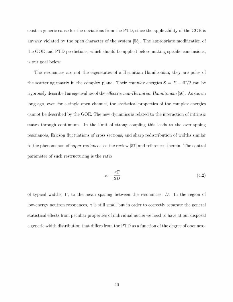
parameter of such restructuring is the ratio
κ =πΓ
2D(4.2)
of typical widths, Γ, to the mean spacing between the resonances, D. In the region of
low-energy neutron resonances, κ is still small but in order to correctly separate the general
statistical effects from peculiar properties of individual nuclei we need to have at our disposal
a generic width distribution that differs from the PTD as a function of the degree of openness.
46

4.2 Resonance width distribution
We need a practical tool that would allow one to compare an experimental output for
an unstable quantum system with predictions of random matrix theory. We propose a
new distribution function that is based, similar to the GOE, on the chaotic character of
time-reversal invariant internal dynamics and corresponding decay amplitudes, but properly
accounts for the continuum coupling through the effective non-Hermitian Hamiltonian.
The numerical simulations for this Hamiltonian were described earlier [51, 58] but here we
derive the analytical expression. In the typical case of nuclear applications, the introduced
dimensionless parameter κ is bound from above by one. The super-radiant regime, κ ≥ 1,
can be of special interest, including such systems as microwave cavities, and in the considered
framework the formal symmetry exists, κ→ 1/κ. At a large number of resonances and fixed
number of open channels, after the super-radiant transition the broad state becomes a part
of the background while the remaining “trapped” states return into the non-overlap regime.
However, in heavy nuclei this transition hardly can be observed because earlier many new
channels can be opened; in the modification of the PTD we see only precursors of this
transition.
Our arguments will follow two different routes which lead to the equivalent results. The
final formula for the statistical width distribution can be presented as
P (Γ) = Cexp
[− N
2σ2 Γ(η − Γ)]
√Γ(η − Γ)
sinh[πΓ2D
(η−Γ)η
]πΓ2D
(η−Γ)η
1/2
. (4.3)
Here we consider N 1 intrinsic states coupled to a single decay channel, for example,
s-wave elastic neutron scattering. The parameter D is a mean energy spacing between the
47

Χ1
2
D = 4D = 2
Cnorm Χ1
2 SinhA Π G
2 DE
Π G2 D
2 4 6 8 10G
0.05
0.10
0.15
0.20
0.25
0.30
PHGL
Figure 4.1: The proposed resonance width distribution according to eq. (4.3) with a singleneutron channel in the practically important case η Γ. The width Γ and mean levelspacing D are measured in units of the mean value 〈Γ〉. “For interpretation of the referencesto color in this and all other figures, the reader is referred to the electronic version of thisdissertation.”
resonances, and C is a normalization constant. The quantity η is the total sum (the trace
of the imaginary part of the effective non-Hermitian Hamiltonian that remains invariant in
the transition to the biorthogonal set of its eigenfunctions) of all N widths; it appears as a
parameter that fixes the starting ensemble distribution, see below eqs. (4.9) and (4.10). The
possible values of widths are restricted from both sides, 0 < Γ < η. The above mentioned
symmetry κ→ 1/κ is reflected in the symmetry Γ→ (η − Γ) of a factor in eq. (4.3) but, as
was already stated, our region of interest is at Γ η. Another parameter, σ, determines the
standard deviation of variable Γ evaluated consistently with the distribution of eq. (4.3). In
48
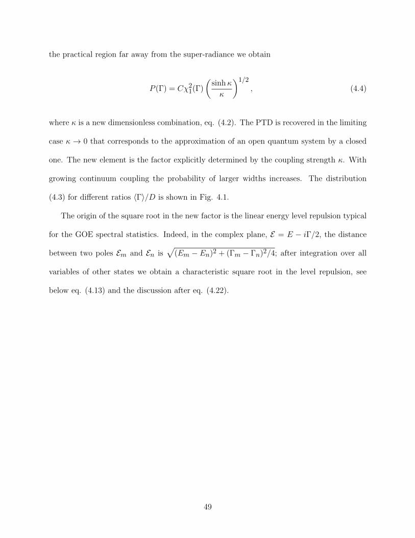
the practical region far away from the super-radiance we obtain
P (Γ) = Cχ21(Γ)
(sinhκ
κ
)1/2
, (4.4)
where κ is a new dimensionless combination, eq. (4.2). The PTD is recovered in the limiting
case κ → 0 that corresponds to the approximation of an open quantum system by a closed
one. The new element is the factor explicitly determined by the coupling strength κ. With
growing continuum coupling the probability of larger widths increases. The distribution
(4.3) for different ratios 〈Γ〉/D is shown in Fig. 4.1.
The origin of the square root in the new factor is the linear energy level repulsion typical
for the GOE spectral statistics. Indeed, in the complex plane, E = E − iΓ/2, the distance
between two poles Em and En is√
(Em − En)2 + (Γm − Γn)2/4; after integration over all
variables of other states we obtain a characteristic square root in the level repulsion, see
below eq. (4.13) and the discussion after eq. (4.22).
49

4.3 Effective non-Hermitian Hamiltonian and
scattering matrix
In order to come to the result (4.3), we start with the general description of complex energies
E = E − iΓ/2 in a system of N unstable states satisfying the GOE statistics inside the
system and interacting with the single open channel through Gaussian random amplitudes.
The general reaction theory [59] is constructed in terms of the elements of the scattering
matrix in the space of open channels a, b, ...,
Sba(E) = δba − iT ba(E). (4.5)
Within the formalism of the effective non-Hermitian Hamiltonian H = H − (i/2)W , the
T -matrix is defined as
T ba(E) =N∑
m,n=1
Ab∗m
[1
E −H
]mn
Aan (4.6)
in terms of the amplitudes Aan connecting an internal basis state n with an open channel
a. Here we do not explicitly indicate the potential part of scattering that is not related to
the internal dynamics of the compound nucleus. The anti-Hermitian part of the effective
Hamiltonian is exactly represented by the sum over k open channels,
Wmn =k∑a=1
AamAa∗n , (4.7)
where the amplitudes can be considered real in the case of time-reversal invariance. It is
important that the factorized structure of the effective Hamiltonian guarantees the unitarity
50

of the scattering matrix. The amplitudes Aan are assumed to be uncorrelated Gaussian
quantities with zero mean and variance defined as AanAbn′ = δabδnn′η/N . The trace of the
anti-Hermitian part of the effective Hamiltonian, η = TrW , i.e. the total sum of all N widths
used in eq. (4.3), is a quantity invariant under orthogonal transformations of the intrinsic
basis. The detailed discussion of the whole approach, numerous applications and relevant
references can be found in the recent review article [57].
The simplest version of the R-matrix description uses instead of the amplitude T ba
its approximate form, where the denominator contains poles on the real energy axis
corresponding to the eigenvalues of the Hermitian part H of the effective Hamiltonian. Then
the continuum coupling occurs only at the entrance and exit points of the process while the
influence of this coupling on the intrinsic dynamics of the compound nucleus is neglected
(in general, the Hermitian part of the Hamiltonian, H, should also be renormalized by the
off-shell contributions from the presence of the decay channels). Contrary to that, the full
amplitude T ba, eq. (4.6), accounts for this coupling during the entire process including
the virtual excursions to the continuum and back from intrinsic states. The poles are the
eigenvalues of the full effective Hamiltonian in the lower half of the complex energy plane.
The experimental treatment corresponds to this full picture. According to the original
experimental paper [44], the R-matrix code SAMMY [60] had been used in the experimental
analysis where the relevant expression is given in the form
Rcc′ =∑λ
γλcγλc′Eλ − E − iΓλ/2
δJJ ′ , (4.8)
and the treatment included a careful segregation of s- and p-resonances, J = J ′ = 1/2 for an
even target nucleus. In the notations of [60] λ represents a particular resonance, Eλ is the
51
energy of the resonance. Here we can identify the intermediate states λ and their complex
energies Eλ− iΓλ/2 with the eigenstates and complex eigenvalues of H, while the numerator
includes the amplitudes transformed to this new basis (under time-reversal invariance the
scattering matrix is symmetric). In terms of the reduced width γ2λc and the penetration
factor Pc, the partial width is Γλc = 2Pcγ2λc. Assuming a single channel and universal
energy dependence of penetration factors, the statistics of the total widths is the same as
that of γ2λc.
4.4 From ensemble distribution to single width
distribution
For a single-channel case, the joint distribution P ( ~E; ~Γ) of all complex energy poles has been
rigorously derived in [55] under assumptions of the GOE intrinsic dynamics in the closed
system and Gaussian distributed random decay amplitudes. The result is given by
P ( ~E; ~Γ) = CN∏m<n
(Em − En)2 +(Γm−Γn)2
4√(Em − En)2 +
(Γm+Γn)2
4
∏n
1√Γn
e−NF ( ~E;~Γ), (4.9)
where the “free energy” F contains interactions of N 1 complex poles in the interval
2a = ND of energies,
F ( ~E; ~Γ) =1
a2
∑n
E2n +
1
2a2
∑m<n
ΓmΓn +1
2η
∑n
Γn. (4.10)
For given N , this distribution contains two parameters, the semicircle radius a for the
intrinsic dynamics and η characterizing the total trace of the imaginary part of the effective
52

Hamiltonian.
Considering this free energy in the “mean-field” approximation, we see that the original
mean value 〈Γ〉0 = η/N is substituted by 〈Γ〉 that is determined by the competition of two
terms, 1/〈Γ〉 = 1/〈Γ〉0 + 〈Γ〉/4D2. The first product in front of exp(−NF ) in eq. (4.9)
substitutes the GOE level repulsion by the repulsion in the complex plane and interaction of
the poles with their negative-Γ “images” [55]. The structure of this result guarantees that
all widths Γ are positive. The formal difficulty with the distribution of eq. (4.9) is that it is
not an analytic function of complex energies.
Our first step is to specify a single N -th pole (EN ,ΓN ) ≡ (E,Γ) and, using the fact that
the distribution ensures Γn ≥ 0, return to the absolute values of the amplitudes,√
Γn = ξn
for other roots. In this form we can apply the steepest descent method owing to a large
parameter N 1 and a saddle point inside the integration interval that was absent in the
initial expression. Integration∏N−1n=1 dξn over all but one variable Γ ≡ ΓN = ξ2
N leads to the
following result for P ( ~E; Γ) as a function of multiple energy variables ~E and a single width
variable Γ
P ( ~E; Γ) = CN∏m<n
|Em − En|∏n
√(En − E)2 +
Γ2
4(4.11)
× exp
[−Na2
(∑n
E2n + E2
)]exp
[−N2ηΓ
]√
Γ
√√√√ 2π
N(
Γa2 + 1
η
)N−1
Introducing new variables, 2a/N = D and λ = ηN , we shall examine the behavior of one of
53

the N -dependent factors in eq. (4.11) in the limit of N →∞,
limN→∞
exp[−N2ηΓ
]√
Γ
(1 +
λΓ
a2N
)−N−12
=exp
[−N2ηΓ
]√
Γexp
[− λ
2a2Γ
](4.12)
The scaling properties of the parameters η, a2, and λ are as follows: η ∝ N , a2 and λ are
both ∝ N2. As a result, the product of two exponents produces a well defined limit that
brings in the desired dependence on the coupling strength κ.
The real energy distribution does not change much in an open system with a single decay
channel being still, at finite but large N , close to a semicircle. We are working in the central
region of the spectrum where the level density is approximately constant and the energy
spectrum is close to equidistant (the maximum of the level spacing distribution is always at
s = δE/D ≈ 1 although the distribution in an open system changes at small spacings, s < 1,
as we will comment later). With En = E − nD, we are able to perform an exact calculation
of the product,
CN∏n
√(En − E)2 +
Γ2
4(4.13)
= CN
N∏n=1
[1 +
Γ2/4
(nD)2
]1/2
N→∞= CN
sinh[π2
ΓD
]π2
ΓD
1/2
,
where we have used the famous Euler formula,
sinhx
x=∞∏k=1
[1 +
x2
k2π2
]. (4.14)
The width-independent factors will enter the normalization constant. Of course, the whole
reasoning is valid in the limit N 1. Finally, the width distribution for Γ η is represented
54

by
P (Γ) = C
sinh[π2
ΓD
]π2
ΓD
1/2exp
[−N2ηΓ
]√
Γexp
[− λ
2a2Γ
]. (4.15)
4.5 Doorway approach
As an alternative derivation, we will apply the doorway approach [38, 61, 62]. Here we use
the eigenbasis of the imaginary part W of the effective non-Hermitian Hamiltonian, eq.
(4.7). Due to the factorized nature of W dictated by unitarity [55], the number of its non-
zero eigenvalues is equal to the number of open channels. In our case we have only one
eigenvalue, the doorway ε0 − iη/2, that has a non-zero width equal to the imaginary part
η of the trace of the Hamiltonian. Remaining basis states are stable being driven by the
Hermitian intrinsic Hamiltonian; its diagonalization produces their real energies εn. These
states acquire the widths through the interaction with the doorway state; the corresponding
matrix elements will be denoted hn. In this basis, the effective Hamiltonian is represented
as
ε0 − i2η h1 h2 · · · hN
h∗1 ε1 0 · · · 0
h∗2 0 ε2 · · · 0
· · · · · · · · · · · · · · ·
h∗N 0 0 · · · εN
. (4.16)
55

The complex eigenvalues E = E − iΓ/2 are the roots of the secular equation,
E = ε0 −i
2η +
N∑n=1
|hn|2E − εn
, (4.17)
that is equivalent to the set of coupled equations for real and imaginary parts,
E = ε0 +N∑n=1
|hn|2E − εn
(E − εn)2 + Γ2/4, (4.18)
Γ =η
1 +∑Nn=1
|hn|2(E−εn)2+Γ2/4
≡ f(Γ, E). (4.19)
For the Gaussian distribution of the coupling matrix elements with 〈|h|2〉 = 2σ2/N (this
scaling was derived in [61]), we obtain
P (Γ) =
∫ +∞
−∞δ (Γ− f(Γ, E)) exp
−Nσ2
N∑n=1
h2n
N∏n=1
dhn. (4.20)
The integration in (4.20) via the steepest descent method leads to eq. (4.3). In order to
get this result we use a possibility to find a highest root E = εN which we set as an origin
relative to which the energies εn can be counted as E = εN , εn = εN − nD. An important
intermediate step is the evaluation of the infinite product of the Lorentzian peaks that can
56

be simplified as
N−1∏n=1
1−Γ2
4 + (E − εN )2
Γ24 + (E − εn)2
−1/2
(4.21)
=
N−1∏n=1
1−Γ2
4
Γ24 + (nD)2
−1/2
=
sinh[π2
ΓD
]π2
ΓD
+1/2
.
In a similar way one can analyze the resonance spacing distribution P (s) along the real
energy axis; spacings s = δE/D are measured in units of their mean value D. As predicted
in [55] and observed numerically in [58], the short-range repulsion disappears and the Wigner
surmise with the standard linear preexponential factor s is substituted by the square root,
P (s) ∝
√s2 + 4
〈Γ2〉D2
exp[− const · s2
]. (4.22)
At spacing s 1, the probability behaves as a+bs2 with the quadratic dependence on s that,
similar to the GUE, mimics the violation of time-reversal invariance due to the open decay
channel. The absence of short-range repulsion, a 6= 0 (the interaction through continuum,
opposite to a normal Hermitian perturbation, repels widths and attracts real energies [63]),
reflects the energy uncertainty of unstable states.
We demonstrated that two complementary approaches which reflect different physical
aspects of the situation lead essentially to the equivalent (after identification of corresponding
parameters) results which we prefer to write in the form (4.3). We expect that for other
canonical ensembles the width distribution far from the super-radiance can be expressed by
a similar formula with the function (sinhκ/κ)β/2, where the standard index of ensemble is
β = 1 for the GOE, β = 2 for the GUE, and β = 4 for the Gaussian Symplectic Ensemble.
57

In the same way we expect the square root in eq. (4.22) to be substituted by the same power
β/2.
The doorway approach naturally indicates the limits of the variable, 0 ≤ Γ ≤ η. It has
also an advantage of the possibility to generalize the answer taking into account explicitly the
rigidity of the internal energy spectrum with fluctuations of level spacings around their mean
value D [in our approximation, only this average value enters eq. (4.3)]. Another direction
of generalization includes the possible influence of a single-particle resonance depending on
a position of its centroid with respect to the considered interval of the resonance spectrum.
In particular, that centroid may be located under threshold of our decay channel. In this
case even the standard energy dependence of the widths can change as was mentioned long
ago [61], see also [50]. The doorway state may or may not coincide with such a resonance
so that the effective Hamiltonian (4.16) may contain two special states coupled with the
“chaotic” background, one by intrinsic interactions and another one through the continuum.
4.6 Photon emission channels
The goal of this section is to estimate in the same spirit the influence of γ-channels on the
resonance width distribution. Only a single open elastic neutron channel was taken into
account in the analysis of data [44,45]. The presence of even weak additional open channels
changes the unitarity conditions. Examples of mutual influence of neutron and gamma
channels are well known in the literature from long ago, see for example [64].
Generalizing the doorway description we allow now each intrinsic state to decay by
gamma-emission which is always possible independently of the position of the neutron
threshold. In the simplest approximation, the effective non-Hermitian Hamiltonian is now
58
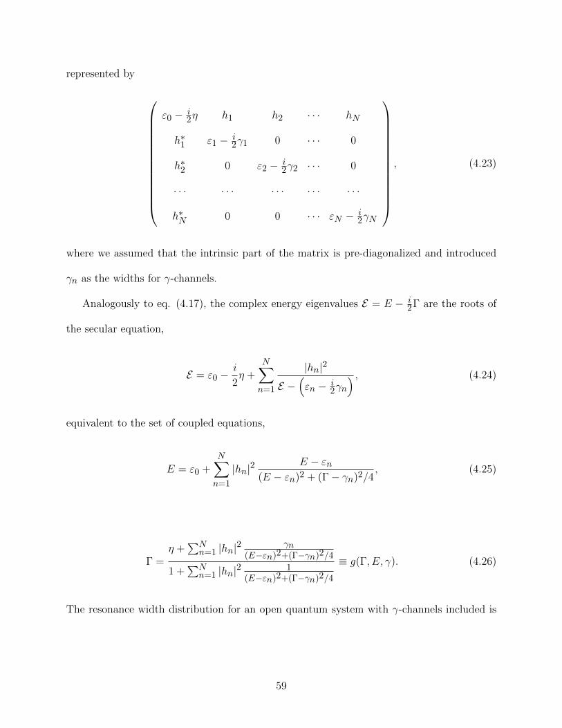
represented by
ε0 − i2η h1 h2 · · · hN
h∗1 ε1 − i2γ1 0 · · · 0
h∗2 0 ε2 − i2γ2 · · · 0
· · · · · · · · · · · · · · ·
h∗N 0 0 · · · εN − i2γN
, (4.23)
where we assumed that the intrinsic part of the matrix is pre-diagonalized and introduced
γn as the widths for γ-channels.
Analogously to eq. (4.17), the complex energy eigenvalues E = E − i2Γ are the roots of
the secular equation,
E = ε0 −i
2η +
N∑n=1
|hn|2
E −(εn − i
2γn
) , (4.24)
equivalent to the set of coupled equations,
E = ε0 +N∑n=1
|hn|2E − εn
(E − εn)2 + (Γ− γn)2/4, (4.25)
Γ =η +
∑Nn=1 |hn|2 γn
(E−εn)2+(Γ−γn)2/4
1 +∑Nn=1 |hn|2 1
(E−εn)2+(Γ−γn)2/4
≡ g(Γ, E, γ). (4.26)
The resonance width distribution for an open quantum system with γ-channels included is
59

Cnorm Χ1
2@G - ΓDSinhA Π HG-ΓL
2 DE
Π HG-ΓL2 D
Χ1
2@GD
D = 2
D = 4
2 4 6 8 10G
0.05
0.10
0.15
0.20
0.25
0.30PHG, ΓL
Figure 4.2: The proposed resonance width distribution according to eq. (4.28) with a singleneutron channel and N gamma-channels in the practically important case η Γ. Theneutron width Γ, radiation width γ, and mean level spacing D are measured in units of themean value 〈Γ〉.
given by
P (Γ, γ) =
∫ +∞
−∞δ (Γ− g(Γ, E, γ)) exp
−Nσ2
N∑n=1
h2n
N∏n=1
dhn. (4.27)
Estimating the gamma-widths by their average value, γ, and acting in the same manner as
in the case of a single open channel we come to the final expression for the resonance width
distribution,
P (Γ, γ) = C(η − γ)√
(Γ− γ)(η − Γ)(4.28)
× exp
[− N
2σ2(Γ− γ)(η − Γ)
]sinh[π(Γ−γ)
2D(η−Γ)η
]π(Γ−γ)
2D(η−Γ)η
1/2
,
60
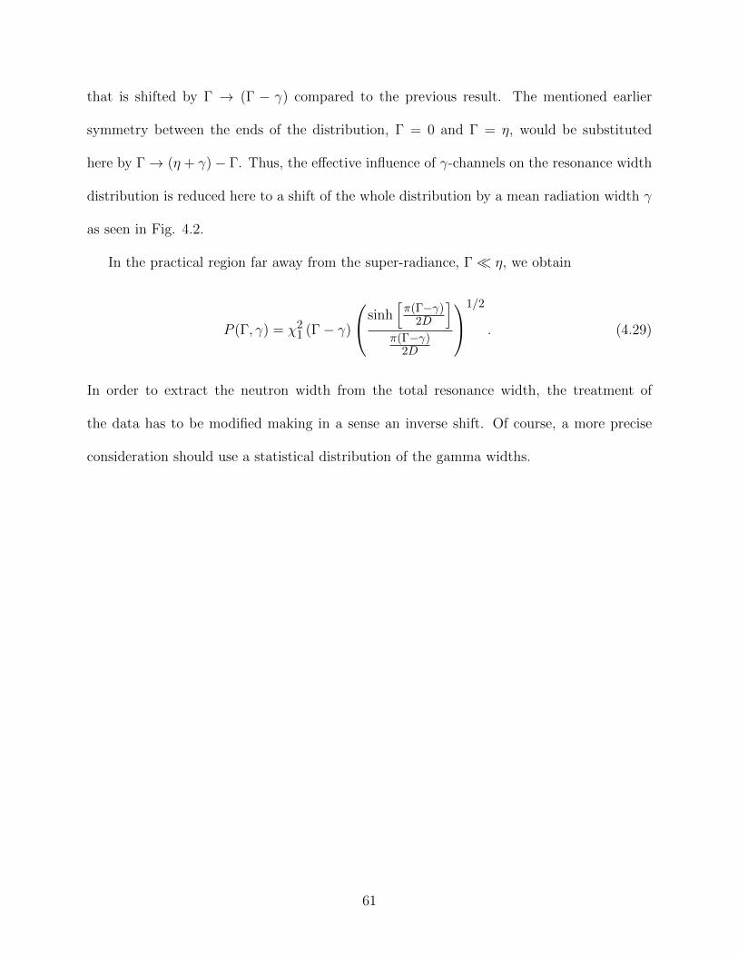
that is shifted by Γ → (Γ − γ) compared to the previous result. The mentioned earlier
symmetry between the ends of the distribution, Γ = 0 and Γ = η, would be substituted
here by Γ→ (η + γ)− Γ. Thus, the effective influence of γ-channels on the resonance width
distribution is reduced here to a shift of the whole distribution by a mean radiation width γ
as seen in Fig. 4.2.
In the practical region far away from the super-radiance, Γ η, we obtain
P (Γ, γ) = χ21 (Γ− γ)
sinh[π(Γ−γ)
2D
]π(Γ−γ)
2D
1/2
. (4.29)
In order to extract the neutron width from the total resonance width, the treatment of
the data has to be modified making in a sense an inverse shift. Of course, a more precise
consideration should use a statistical distribution of the gamma widths.
61

4.7 Many-channel case
In the two-channel case the effective Hamiltonian is
ε0 − i2η0 h1 h2 h3 · · · hN
h∗1 ε1 − i2η1 v2 v3 · · · vN
h∗2 v∗2 ε2 0 · · · 0
· · · · · · · · · · · · · · · · · ·
h∗N v∗N 0 0 · · · εN
. (4.30)
It can be shown that the Schrodinger equation with Hamiltonian eq. (4.30) for complex
eigenvalue Eα = Eα − i2Γα can be rewritten in terms of matrix
A =
∑Nk=2
h2k
εk−Eα+ Eα − (ε0 − iη0
2 ) h1 −∑Nk=2
hkvkεk−Eα
h1 −∑Nk=2
hkvkεk−Eα
∑Nk=2
v2k
εk−Eα+ Eα − (ε1 − iη1
2 )
, (4.31)
namely the secular equation for the Hamiltonian eq. (4.30) is equivalent to
detA = 0. (4.32)
We shall note that in the general case dimension of the corresponding matrix A is equal to
the number of open channels, i.e. number of rows (or columns) k with random variables in
the original Hamiltonian (see Appendix B).
62

Following the general procedure we get the equation for the width,
Γ =
E(η0+η1)2 − ε1η0+ε0η1
2E − ε0+ε12 −∑k
v2kε0+h2
kε1
2
(Γ24 +(E−εk)2
) +∑k
E(v2k
+h2k
)
2
(Γ24 +(E−εk)2
)
≡ f(Γ, hk, vk). (4.33)
By averaging the width Γ, eq. (4.33), over the set of random variables hn and vn we get the
width distribution,
P (Γ) =
∫ +∞
−∞δ (Γ− f(Γ, hn, vn))
× exp
−Nσ2
N∑n=1
h2n
N∏n=1
dhn exp
−Nσ2
N∑n=1
v2n
N∏n=1
dvn. (4.34)
Introducing k = 2 dimensional spherical coordinates
r2N ≡ v2
N + h2N (4.35)
and taking into account
Vk(R) =πk2
Γ[k2 + 1
]Rk, (4.36)
dVk(R) =πk2
Γ[k2 + 1
]kRk−1dR ' CkRk−1dR,
63

we obtain
P (Γ) =
∫ +∞
−∞
N−1∏n=1
dhn
N−1∏n=1
dvnδ (Γ− f(Γ, hn, vn)) (4.37)
× exp
−Nσ2
N−1∑n=1
h2n
exp
−Nσ2
N−1∑n=1
v2n
exp
[−N r2
N
σ2
]πk2
Γ[k2 + 1
]krk−1N drN .
The Dirac δ-function produces a derivative in the denominator which behaves as
∣∣∣∣ dΓ
drN
∣∣∣∣ = CrN∑k
i=1 ηi/k. (4.38)
After applying the steepest descent method and in the particular case k = 2 after smoke
clears we have
P (Γ) = C exp
[− N
2σ2Γ
(η0 + η1
2− Γ
)]× φ
(Γ
D
), (4.39)
which, except for the factor φ (Γ/D), is nothing but χ2k
[Γ(η0+η1
2 − Γ)]
distribution in case
of k = 2 open channels. The factor φ (Γ/D) is evaluated by means of the Euler formula and
is given in terms of the sum of partial width η,
η =
∑ki=1 ηik
, (4.40)
and the number of open channels k,
φ
(Γ
D
)=
sinh[πΓ2D
(η−Γ)η
]πΓ2D
(η−Γ)η
k2
. (4.41)
64

In the general case of k open channels the width distribution is
P (Γ) = C exp
[− N
2σ2Γ (η − Γ)
](Γ (η − Γ))
k−22
sinh[πΓ2D
(η−Γ)η
]πΓ2D
(η−Γ)η
k2
. (4.42)
4.8 Conclusion
In this chapter we proposed a new resonance width distribution for an open quantum
system based on chaotic intrinsic dynamics and coupling of states with the same quantum
numbers to the common decay channel. Two approximate methods lead to an equivalent
analytical expression for the width distribution that does not belong to the class of chi-
square distributions with the only parameter ν traditionally used in the analysis of data.
In the limit of vanishing openness and return to a closed system we recover the standard
PTD. The new result depends on the ratio (4.2) of the width to the mean level spacing,
κ ∼ Γ/D, that regulates the strength of the continuum coupling. The deviations from the
PTD grow with κ up to the critical strength κ ∼ 1, when the broad “super-radiant” state
becomes essentially the part of the background, while the remaining “trapped” states return
to the weak coupling regime. This physics was repeatedly discussed previously, especially in
relation to quantum signal transmission through mesoscopic devices [57,65], but it is outside
of our interest here.
In the practical region of low-energy neutron resonances, the effects predicted here are
relatively small. Although at small κ the derived neutron width distribution supports an
experimental trend, the final judgment can be made only after the presence of gamma-
channels was accounted for. We have to attract the attention of experimentalists to the fact
that the data should be analyzed with the aid of the distribution that does not belong to the
65

routinely used chi-square class; gamma channels should be included into consideration. We
can also mention that the result agrees with numerical simulations [51] for the full many-
resonance distribution function (4.9). Using the suggested distribution as a new reference
point, one can ascribe the remaining deviations to the specific features of individual systems
(level densities, single-particle structure in a given energy region, shape transformations,
energy dependence of the widths etc.). Unfortunately, we still do not have experimental
tests for the full distribution (4.9). Although in nuclear physics it is hard to make such a
detailed analysis for higher energies and greater degree of resonance overlap, the systems
with tunable chaos, such as microwave cavities, acoustic blocks, or even elastomechanical
devices [66], seem to provide appropriate tools for such studies.
66
Chapter 5
Cosmology
In this chapter we present analytical solution for time evolution of the gravitational wave
damping in the early Universe due to freely streaming neutrinos in both early-time and late-
time limit, as well as for the general case. In the extreme cases of early-time and late-time
limits, the solution is represented by a convergent series of spherical Bessel functions of even
order, which is not the case for the general solution. The derivation was possible with the
help of a new compact formula for the convolution of spherical Bessel functions of integer
order.
The results of this chapter are based on our work,
GS, arXiv:1204.1384 (2012).
5.1 Introduction
Thorough analysis of cosmic microwave background (CMB) radiation provides a unique test
for the standard inflationary cosmological model [67–72]. While scalar fluctuations of CMB
serve as an invaluable source for exploring density of matter and radiation and large-scale
structure of the universe [73–78], observations of tensor fluctuations of CMB open a window
for searching after a signature of gravitational waves [79–82].
The CMB observations done by Wilkinson Microwave Anisotropy Probe (WMAP) [83]
67

generally support theoretical predictions based on the standard inflationary cosmological
model. The detailed analysis of the experimental data provides more and more accurate
values [84–86] for the most valuable cosmological parameters, such as baryon density, total
matter density, Hubble constant, and age of the Universe.
Independently of WMAP measurements, there is a long quest for a direct observation
of cosmological gravitational waves [87]. The specially designed for this task Laser
Interferometer Gravitational Wave Observatory (LIGO) puts a major effort in this
experimental challenge [88]. A direct observation of cosmological gravitational waves would
serve as a decisive test for validity of the Einstein general theory of relativity in the same
way as the Michelson - Morley experiment served as a major proof for the Einstein special
theory of relativity.
In this chapter we analyze the problem of gravitational wave damping in the early
Universe due to freely streaming neutrinos in both early and late-time regime. The exact
solution in the early-time limit is given by a convergent series of spherical Bessel functions
of even order. In this limit the solution is independent of dimensionless parameter of
momentum Q. The neutrino source perturbation does not change the qualitative behavior of
the homogeneous gravitational wave damping solution but effectively changes its amplitude
from unity to the corresponding asymptotic value.
The late-time limit solution is represented by a convergent series of spherical Bessel
functions of even order and is Q-independent for large values of Q. Thus the prediction made
by S. Weinberg concerning the Q-independent solution for the gravitational wave damping
given by a series of even spherical Bessel functions is valid in both early and late-time limit.
S. Weinberg’s predictions fails in the general case where we were able to construct the
solution in terms of an infinite series of the product of spherical Bessel function and reciprocal
68

sum of the time parameter u and the parameter Q. Even though for large Q-values the series
coefficients of the proposed solution are Q-independent, the solution for the gravitational
wave damping depends on Q-value, and in general is represented by a linear combination of
both even and odd spherical Bessel functions.
The constructed solution for the general case was possible due the nontrivial equality for
the differential operator of the gravitational wave damping problem which upon its action
onto the trial function returns the exact sum of its action onto the function in the early and
late-time limits, which we consider as the main result of the present investigation.
5.2 Fluctuations in General Relativity
In this section we are interested in the Einstein field equation for the traceless and
divergenceless part of the metric perturbation tensor hij(x, t) for the metric tensor gµν ,
defined as
g00 = −1, (5.1)
gi0 = 0,
gij(x, t) = a2(t)δij + hij(x, t),
where a(t) is the Robertson--Walker scale factor, which measures the expansion rate of the
Universe.
In the subsequent section we derive the kinetic Boltzmann equation for the neutrino
energy-momentum tensor πTij which will be given in terms of the metric perturbation tensor
hij(x, t). Finally we obtain the integro-differential equation for the metric perturbation
69

hij(x, t) which we subsequently build solution for.
The Einstein field equation,
Rµν = −8πGSµν , (5.2)
is given in terms of the Ricci tensor Rµν ,
Rµν =∂Γλλµ∂xν
−∂Γλµν
∂xλ+ ΓλµσΓσνλ − ΓλµνΓσλσ, (5.3)
the shifted energy-momentum tensor Sµν ,
Sµν = Tµν −1
2gµνg
ρσTρσ, (5.4)
and Newton gravitational constant G. Here we have introduced the field Γλµν known as the
affine connection,
Γλµν =1
2gλρ
[∂gρµ∂xν
+∂gρν∂xµ
− ∂gµν∂xρ
]. (5.5)
Below we introduce the unperturbed metrics and energy-momentum tensor which we label
by a horizontal bar.
First we introduce the unperturbed Robertson–Walker metrics,
g00 = −1, (5.6)
gi0 = g0i = 0,
gij(t) = a2(t)δij ,
70
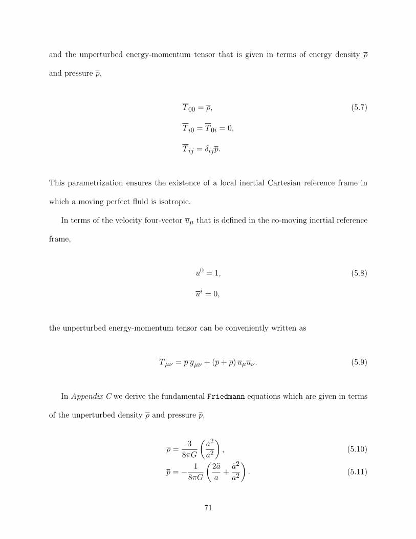
and the unperturbed energy-momentum tensor that is given in terms of energy density ρ
and pressure p,
T 00 = ρ, (5.7)
T i0 = T 0i = 0,
T ij = δijp.
This parametrization ensures the existence of a local inertial Cartesian reference frame in
which a moving perfect fluid is isotropic.
In terms of the velocity four-vector uµ that is defined in the co-moving inertial reference
frame,
u0 = 1, (5.8)
ui = 0,
the unperturbed energy-momentum tensor can be conveniently written as
Tµν = p gµν + (p+ ρ)uµuν . (5.9)
In Appendix C we derive the fundamental Friedmann equations which are given in terms
of the unperturbed density ρ and pressure p,
ρ =3
8πG
(a2
a2
), (5.10)
p = − 1
8πG
(2a
a+a2
a2
). (5.11)
71
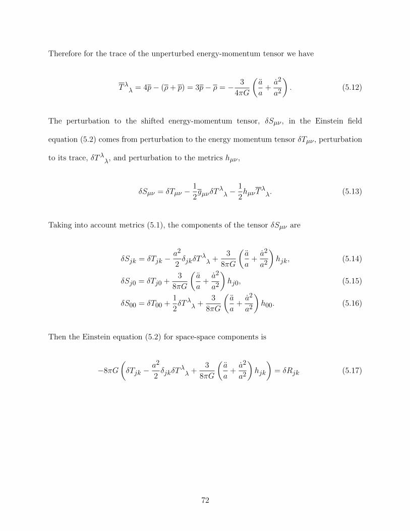
Therefore for the trace of the unperturbed energy-momentum tensor we have
Tλλ = 4p− (ρ+ p) = 3p− ρ = − 3
4πG
(a
a+a2
a2
). (5.12)
The perturbation to the shifted energy-momentum tensor, δSµν , in the Einstein field
equation (5.2) comes from perturbation to the energy momentum tensor δTµν , perturbation
to its trace, δTλλ, and perturbation to the metrics hµν ,
δSµν = δTµν −1
2gµνδT
λλ −
1
2hµνT
λλ. (5.13)
Taking into account metrics (5.1), the components of the tensor δSµν are
δSjk = δTjk −a2
2δjkδT
λλ +
3
8πG
(a
a+a2
a2
)hjk, (5.14)
δSj0 = δTj0 +3
8πG
(a
a+a2
a2
)hj0, (5.15)
δS00 = δT00 +1
2δTλλ +
3
8πG
(a
a+a2
a2
)h00. (5.16)
Then the Einstein equation (5.2) for space-space components is
−8πG
(δTjk −
a2
2δjkδT
λλ +
3
8πG
(a
a+a2
a2
)hjk
)= δRjk (5.17)
72

with the perturbation to the Ricci tensor
δRjk = −1
2∂j∂kh00 − (2a2 + aa)δjkh00 −
1
2aaδjkh00 (5.18)
+1
2a2
(∇2hjk − ∂i∂jhik − ∂i∂khij + ∂j∂khii
)−1
2hjk +
a
2a(hjk − δjkhii) +
(a2
a2
)(−2hjk + δjkhii) +
a
aδjk∂ihi0
+1
2(∂j hk0 + ∂khj0 +
a
2a(∂jhk0 + ∂khj0).
The next step is to introduce the most general parametrization for the metrics perturbation,
hij = a2[Aδij +
∂2B
∂xi∂xj+∂Ci∂xj
+∂Cj
∂xi+Dij
], (5.19)
hi0 = a
[∂F
∂xi+Gi
], (5.20)
h00 = −E. (5.21)
For the traceless and divergenceless tensor perturbation,
∂Dij
∂xi= 0, (5.22)
Dii = 0, (5.23)
Dij = Dji, (5.24)
we are left only with
hij = a2Dij , (5.25)
while all other terms contribute only to scalar and vector perturbations. As a consequence,
73

the metrics perturbation tremendously simplifies to
3
(a
a+a2
a2
)hjk + δRjk =
1
2a2∇2hjk −
1
2hjk +
a
2ahjk +
(3a
a+a2
a2
)hjk
=1
2∇2Djk −
a
2
(3aDjk + aDjk
). (5.26)
The most general perturbation to the energy-momentum tensor can be written as
δTij = phij + a2[δijδp+ ∂i∂jπ
S + ∂iπVj + ∂jπ
Vi + πTij
], (5.27)
δTi0 = phi0 − (ρ+ p)(∂iδu+ δuVi
), (5.28)
δT00 = −ρh00 + δρ. (5.29)
where πS , πVj , and πTij are the scalar, vector and tensor perturbations, correspondingly. For
the perturbation to the energy-momentum tensor δTµν , there is only a single term πTij , which
satisfies the traceless and divergenceless conditions,
∂πTij
∂xi= 0, (5.30)
πTii = 0, (5.31)
πTij = πTji. (5.32)
The explicit form of the tensor perturbation πTij will be found from the kinetic Boltzmann
equation in the subsequent section.
Finally we arrive at the desirable Einstein field equation for the metrics perturbation
74

mode Djk [89],
∇2Djk − a2Djk − 3aaDjk = −16πGa2πTjk. (5.33)
The obtained equation governs the metric perturbation tensor Djk that is driven by the
energy-momentum tensor perturbation πTjk.
5.3 Boltzmann equation for neutrinos
In this section our main interest is to obtain the neutrino energy-momentum tensor
perturbation πTjk from the Boltzmann equation. Following S. Weinberg [89] we argue that
the velocity of cold dark matter and baryonic plasma is too slow to make a contribution to
anisotropic inertia tensor. Therefore the only contributions to the anisotropic inertia tensor
are due to photons and neutrinos. Photons, however, have a short mean free time before the
era of recombination [89], and therefore their contribution to the anisotropic inertia tensor is
relatively small. As the result, we are left with neutrinos, which we assume to be massless,
that represent the main source for perturbation to the anisotropic inertia tensor.
First we define the neutrino distribution function in the phase space as
nν(x,p, t) ≡∑r
[3∏i=1
δ(xi − xir(t)
) 3∏i=1
δ(pi − pir(t)
)], (5.34)
where r labels a neutrino trajectory. From the momentum definition
pµr =
dxµr
dur, (5.35)
75
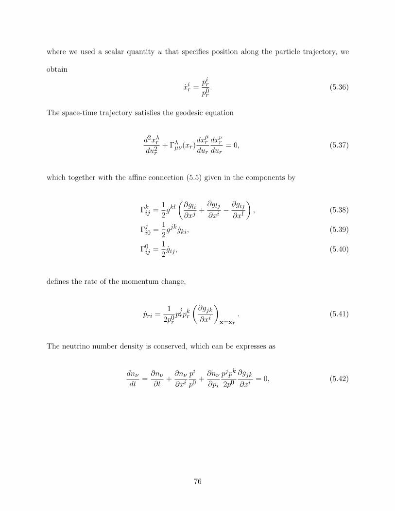
where we used a scalar quantity u that specifies position along the particle trajectory, we
obtain
xir =pirp0r. (5.36)
The space-time trajectory satisfies the geodesic equation
d2xλrdu2r
+ Γλµν(xr)dxµr
dur
dxνrdur
= 0, (5.37)
which together with the affine connection (5.5) given in the components by
Γkij =1
2gkl(∂gli∂xj
+∂glj
∂xi− ∂gij
∂xl
), (5.38)
Γji0 =
1
2gjkgki, (5.39)
Γ0ij =
1
2gij , (5.40)
defines the rate of the momentum change,
pri =1
2p0rpjrpkr
(∂gjk
∂xi
)x=xr
. (5.41)
The neutrino number density is conserved, which can be expresses as
dnνdt
=∂nν∂t
+∂nν
∂xipi
p0+∂nν∂pi
pjpk
2p0
∂gjk
∂xi= 0, (5.42)
76

where we we have introduced the standard notations,
pi = gij(x, t)pj , (5.43)
p0 =√gij(x, t)pipj .
Our goal is to derive the kinetic Boltzmann equation in the first order in metrics and
density perturbation, δgij(x, t) and δnν(x, t), correspondingly. In the following we denote
an arbitrary perturbation to the metrics as
gij(x, t) = a2(t)δij + δgij(x, t). (5.44)
For the perturbation of the neutrino density we have
nν(x, t) = nν [a(t)p] + δnν(x, t), (5.45)
nν(p) =1
(2π)3
1
exp
[pa(t)
1kT (t)
]+ 1
. (5.46)
Then the Boltzmann equation for neutrinos to the first order in perturbations reads
∂δnν(x,p, t)
∂t+∂δnν(x,p, t)
∂xipi
a(t)p(5.47)
+n′ν(p)
2p
∂
∂t
(a2(t)δgij(x, t)
)pipj +
n′ν(p)
2p
∂
∂xk
(a2(t)δgij(x, t)
)pipj
pka(t)p
+n′ν(p)pipjpk
2a3(t)p2
∂
∂xk
(δgij(x, t)
)= 0,
where
n′ν(p) =∂nν(p)
∂p. (5.48)
77

Up to the first order the inverse metric tensor is
gij =1
a2δij −
1
a4δgij , (5.49)
and we can greatly simplify the Boltzmann equation due to the following cancellation:
n′ν(p)
2p
∂
∂xk
(a2(t)δgij(x, t)
)pipj
pka(t)p
+ n′ν(p)pipjpk
2a3(t)p2
∂
∂xk
(δgij(x, t)
)(5.50)
=
(− 1
a2(t)
)n′ν(p)
pipjpk2a(t)p2
∂
∂xk
(δgij(x, t)
)+ n′ν(p)
pipjpk2a3(t)p2
∂
∂xk
(δgij(x, t)
)= 0.
Therefore we are left with
∂δnν(x,p, t)
∂t+∂δnν(x,p, t)
∂xipi
a(t)p=n′ν(p)
2ppipj
∂
∂t
(1
a2(t)δgij(x, t)
). (5.51)
Introducing the tensor perturbation
δgij(x, t) = hij(x, t) = a2Dij(x, t), (5.52)
and the unit vector along the momentum
pi =pip, (5.53)
p ≡ √pipi, (5.54)
we arrive at the Boltzmann equation in the coordinate space,
∂δnν(x,p, t)
∂t+∂δnν(x,p, t)
∂xipia(t)
=1
2pn′ν(p)pipjDij(x, t). (5.55)
78

The next step is to introduce a dimensionless intensity perturbation J(x, p, t),
a4(t)ρν(t)J(x, p, t) ≡ Nν
∫ ∞0
δnν(x,p, t)p3dpd2p, (5.56)
ρν(t) ≡ Nνa4(t)
∫ ∞0
dpnν(p)4πp3. (5.57)
Multiplying the Boltzmann equation (5.55) by p3dpd2p with subsequent integration over
momentum p and performing integration by parts, we obtain for the right hand side
1
2pipjDij(x, t)
∫ ∞0
dpn′ν(p)4πp4 = −2pipjDij(x, t)
∫ ∞0
dpnν(p)4πp3
= −2pipjDij(x, t)ρν(t)a4(t)
Nν. (5.58)
As the result, the Boltzmann equation for the dimensionless neutrino density J(x, p, t) is [89]
∂J(x, p, t)
∂t+
pia(t)
∂J(x, p, t)
∂xi= −2pipjDij(x, t). (5.59)
79
5.4 Momentum representation
Now we have all the tools we need to build the solution of the Boltzmann equation for the
neutrino density. We introduce a stochastic amplitude for the single non-decaying mode
with the wave number q and helicity λ,
β(q, λ), (5.60)
together with its local correlation,
〈β(q, λ)β∗(q′, λ′)〉 = δλλ′δ3 (q− q′
). (5.61)
Also we need the polarization tensor
eij(q, λ), (5.62)
satisfying the traceless and divergenceless conditions automatically,
eii = 0, (5.63)
qieij = 0. (5.64)
In the following we transform the obtained Boltzmann equation (5.59) into the momentum
representation.
First we need to introduce the notion of helicity, labeled by λ. The wave propagating
in the direction k is said to have a helicity λ if it bears an angular momentum hλ in the
direction of flight. The traceless and divergenceless conditions for the metric perturbation
80

tensor in the momentum representation Dqij are
Dqij = D
qji, (5.65)
Dqii = 0, (5.66)
qiDqij = qjD
qij = 0. (5.67)
Under the rotation by an angle θ, the metric perturbation tensor in the momentum
representation Dqij transforms as
Dq11 ∓D
q12 −→ eiλθ
[Dq11 ∓D
q12
], (5.68)
λ = ±2.
Further we introduce the Fourier representation for the metric perturbation tensor Dij(x, t),
Dij(x, t) =∑λ=±2
∫d3q exp (iqx)β(q, λ)eij(q, λ)Dq(t), (5.69)
the Fourier representation for the anisotropic inertia tensor πTij(x, t),
πTij(x, t) =∑λ=±2
∫d3q exp (iqx)β(q, λ)eij(q, λ)πTq (t), (5.70)
and the Fourier representation for dimensionless neutrino density function J(x, p, t),
J(x, p, t) =∑λ=±2
∫d3q exp (iqx)β(q, λ)eij(q, λ)pipjJq(q, p · q, t). (5.71)
As the result, the momentum representation of the Boltzmann equation (5.59) for the
81

neutrino density Jq(q, p · q, t) becomes the first-order differential equation,
Jq(q, p · q, t) + ip · q q
a(t)Jq(q, p · q, t) = −2Dq(t). (5.72)
Performing a simple algebra with an integrating factor,
exp
[−iqp · q
∫ t
t0
dt′′
a(t′′)
]∫ t
t0
dt′ exp
[iqp · q
∫ t′
t0
dt′′
a(t′′)
]Dq(t
′) (5.73)
=
∫ t
t0
dt′ exp
[−iqp · q
∫ t
t′dt′′
a(t′′)
]Dq(t
′),
we obtain the solution of the Boltzmann equation for the neutrino density,
Jq(q, p · q, t) = −2
∫ t
t0
dt′ exp
[−iqp · q
∫ t
t′dt′′
a(t′′)
]Dq(t
′). (5.74)
82

5.5 Perturbations to the energy-momentum tensor
In this section we shall find the neutrino stress-energy tensor in the momentum representation
πTq (t). The first-order perturbations to the energy-momentum tensor are
δT ij =1
a4(t)
∫ (3∏
k=1
dpk
)δnν(x,p, t)
pipjp, (5.75)
δT 0j =
1
a4(t)
∫ (3∏
k=1
dpk
)δnν(x,p, t)pj , (5.76)
δT 00 =
1
a4(t)
∫ (3∏
k=1
dpk
)δnν(x,p, t)p. (5.77)
For our purpose we need only the tensor part δT ij that can be simplified as
δT ij =1
a4(t)
∫ (3∏
k=1
dpk
)a2(t)δnν(x,p, t)ppipj . (5.78)
Recalling the definition of the dimensionless intensity perturbation J(x, p, t), eq. (5.56), we
obtain for the tensor perturbation δT ij
δT ij = (5.79)
=1
a4(t)
∫ (3∏
k=1
dpk
)δnν(x,p, t)ppipj = ρν(t)
∫d2p
4πJ(x, p, t)pipj
= ρν(t)∑λ=±2
∫d3q exp (iqx)β(q, λ)ekl(q, λ)
∫d2p
4πpipj pkplJq(q, p · q, t).
The algebra of the polarization tensor ekl(q) simplifies the task,
∫d2p f(p · q)pipkejk(q) =
1
2eij(q)
∫d2p f(p · q)
(1− (p · q)2
), (5.80)
83

∫d2p f(p · q)pipj pkplekl(q) =
1
4eij(q)
∫d2p f(p · q)
(1− (p · q)2
)2. (5.81)
As the result we have for the tensor perturbation
δT ij = ρν(t)∑λ=±2
∫d3q exp (iqx)β(q, λ)eij(q) (5.82)
×1
4
∫d2p
4π
(1− (p · q)2
)2Jq(q, p · q, t),
and with the obtained earlier solution of the Boltzmann equation for the neutrino density
Jq(q, µ, t), eq. (5.74), we have
δT ij = ρν(t)∑λ=±2
∫d3q exp (iqx)β(q, λ)eij(q) (5.83)
×(−2
4
)∫d2p
4π
(1− (p · q)2
)2∫ t
t0
dt′ exp
[−iq(p · q)
∫ t
t′dt′′
a(t′′)
]Dq(t
′).
In the obtained expression for the tensor perturbation we can perform the surface integration
I(u) ≡∫d2p
4π
(1− (p · q)2
)2exp
[−iq(p · q)
∫ t
t′dt′′
a(t′′)
]. (5.84)
Introducing the time variable u and the angle variable s,
u = q
∫ t
t′dt′′
a(t′′), (5.85)
s = (p · q), (5.86)
and, owing to the azimuthal symmetry,
d2p = 2πds, (5.87)
84

we express the surface integral I(u) in terms of spherical Bessel functions jn(u),
I(u) =
∫ 1
−1
ds
2
(1− s2
)2exp [−ius]
=
(− 8
u5
)[3u cosu+
(u2 − 3
)sinu
]= 8
j2(u)
u2= 8
(1
15j0(u) +
2
21j2(u) +
1
35j4(u)
). (5.88)
Finally the tensor perturbation simplifies to
δT ij =∑λ=±2
∫d3q exp (iqx)β(q, λ)eij(q) (5.89)
×(−4)ρν(t)
∫ t
t0
dt′K(q
∫ t
t′dt′′
a(t′′)
)Dq(t
′),
with the kernel
K(u) ≡ 1
15j0(u) +
2
21j2(u) +
1
35j4(u). (5.90)
Recalling the momentum representation of the anisotropic inertia tensor πTij(x, t), eq. (5.70),
we arrive at the neutrino stress-energy tensor in the momentum representation
πTq (t) = −4ρν(t)
∫ t
0dt′K
(q
∫ t
t′dt′′
a(t′′)
)Dq(t
′). (5.91)
In terms of the time variable u it looks like [89]
πTq (u) = −4ρν(u)
∫ u
0dUK (u− U)D′q(U), (5.92)
which is nothing but the convolution integral of the kernel K(u), eq. (5.90), and the time
derivative of the metrics perturbation Dq(u).
85

5.6 Gravitational wave damping
The Einstein field equation for the tensor perturbation is given by eq. (5.33). Recalling the
Fourier representations for the metric perturbation tensor Dij(x, t), eq. (5.69), and for the
anisotropic inertia tensor πTij(x, t), eq. (5.70), we obtain the gravitational wave damping
equation in the momentum representation
Dq(t) +3a
aDq(t) +
q2
a2Dq(t) = −64πGρν(t)
∫ t
0dt′K
(q
∫ t
t′dt′′
a(t′′)
)Dq(t
′), (5.93)
where the kernel K(u) is given by (5.90). In terms of the time variable u, eq. (5.85), the left
hand side of the gravitational wave equation transforms as
Dq(t) +3a
aDq(t) +
q2
a2Dq(t) (5.94)
=
(q
a(u)
)2 [D′′q (u) + 2
(a′(u)
a(u)
)D′q(u) +Dq(u)
].
As the result, we obtain the gravitational wave equation entirely in terms of the variable u,
D′′(u) + 2
(a′(u)
a(u)
)D′(u) +D(u) (5.95)
= −64πG
(a(u)
q
)2
ρν(u)
∫ u
0dUK (u− U)D′(U).
In terms of the Hubble expansion rate,
H(t) =a(t)
a(t), (5.96)
86

and the time variable u, the Friedmann equation for the unperturbed energy density ρ
becomes
ρ =3
8πGH2(t) =
3
8πG
(a2(t)
a2(t)
)=
3
8πG
(q
a(u)
a′(u)
a(u)
)2
, (5.97)
and therefore the energy-momentum prefactor in eq. (5.95) can be expressed as
−64πG
(a(u)
q
)2
ρν(u) (5.98)
= −64πG
(a(u)
q
)2
H2(t)ρν(u)
ρ
3
8πG= −24
ρν(u)
ρ
(a′(u)
a(u)
)2
.
Finally we obtain the gravitational wave equation
D′′(u) + 2
(a′(u)
a(u)
)D′(u) +D(u) = −24
ρν(u)
ρ
(a′(u)
a(u)
)2 ∫ u
0dUK (u− U)D′(U). (5.99)
The unperturbed equilibrium neutrino and photon energy density, ρν(u) and ργ(u),
correspondingly, define the ratio
fν(0) ≡ ρν(u)
ρ=
ρνρν + ργ
=3(
78
)(411
)4/3
1 + 3(
78
)(411
)4/3' 0.40523, (5.100)
which we refer to Appendix D for details.
It is convenient to use the dimensionless quantity
y ≡ a(t)
aeq, (5.101)
aeq = a(t = teq),
87

where teq is the time of matter-radiation equality, which will be discussed in the next section.
Introducing Q as the ratio of the wave number to its value at the time of matter-radiation
equality,
Q =√
2q
qeq, (5.102)
qeq = aeqHeq,
and owing to
du
dy=
Q√1 + y
, (5.103)
we obtain
(1 + y)d2D(y)
dy2+
(2(1 + y)
y+
1
2
)dD(y)
dy+Q2D(y) (5.104)
= −24fν(0)
y2
∫ y
0K(
2Q(√
1 + y −√
1 + y′)) dD(y′)
dy′dy′.
With the change of variable
y =u(u+ 4Q)
4Q2, (5.105)
we may rewrite the obtained equation in a more convenient form,
d2D(u)
du2+
(4(u+ 2Q)
u(u+ 4Q)
)dD(u)
du+D(u) (5.106)
= −24fν(0)
(4Q
u(u+ 4Q)
)2 ∫ u
0K(u− U)
dD(U)
dUdU,
88

with the kernel K(u) given by eq. (5.90), and the initial conditions
D(0) = 1, (5.107)
dD(u)
du
∣∣∣∣u=0
= 0.
5.7 Matter-radiation equality
Matter-radiation equality corresponds to moment at which ratio of the co-moving
wavenumber q to the expansion rate a becomes equal to the Hubble expansion rate H,
q
a(t)= H(t), (5.108)
t ≡ teq. (5.109)
By integrating eq. (5.108) over time we can express the matter-radiation equality in terms
of the time variable u,
u(teq) = q
∫ teq
0
dt′
a(t′)=
∫ teq
0H(t′)dt′ =
∫ teq
0
a(t′)a(t′)
dt′ = ln
[a(teq)
a(0)
](5.110)
The early-time limit, u Q, that corresponds to the long wavelengths, or equivalently to
the lower-bound wavenumbers q qeq, while the late-time limit, u Q, that is referred to
the short wavelengths, corresponds to the upper-bound wavenumbers q qeq.
In order to find the value for qeq we must recall the black-body spectrum, which is
formulated in terms of the number density of photons nT (ν) being in equilibrium with
89
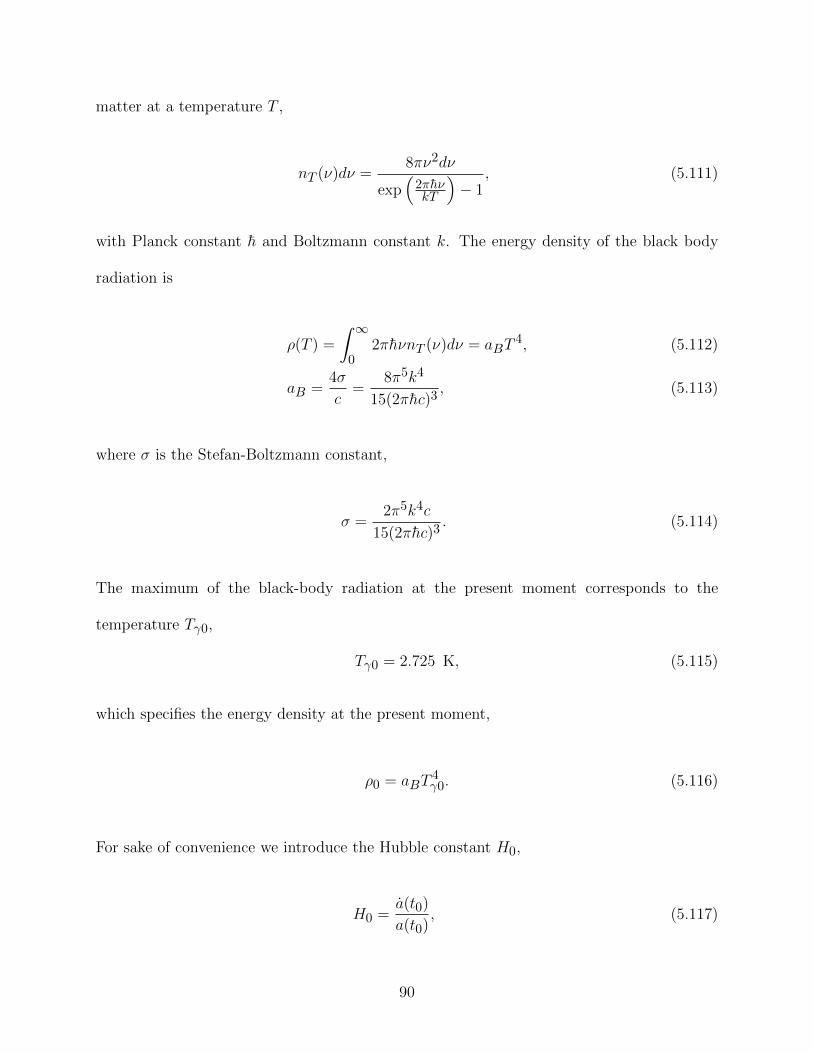
matter at a temperature T ,
nT (ν)dν =8πν2dν
exp(
2πhνkT
)− 1
, (5.111)
with Planck constant h and Boltzmann constant k. The energy density of the black body
radiation is
ρ(T ) =
∫ ∞0
2πhνnT (ν)dν = aBT4, (5.112)
aB =4σ
c=
8π5k4
15(2πhc)3, (5.113)
where σ is the Stefan-Boltzmann constant,
σ =2π5k4c
15(2πhc)3. (5.114)
The maximum of the black-body radiation at the present moment corresponds to the
temperature Tγ0,
Tγ0 = 2.725 K, (5.115)
which specifies the energy density at the present moment,
ρ0 = aBT4γ0. (5.116)
For sake of convenience we introduce the Hubble constant H0,
H0 =a(t0)
a(t0), (5.117)
90

in units of 100 kms Mpc and denote it as h,
h = H0 ×(
100km
s Mpc
)−1
. (5.118)
In the general case the critical energy density ρ is given by the Friedmann equation and it
consists of a mixture of vacuum energy, non-relativistic matter, and radiation,
ρ =3
8πGH2
0
[ΩΛ + ΩM
(a0
a
)3+ ΩR
(a0
a
)4], (5.119)
where present date quantities are labeled by a zero index. The present values for energy
density of vacuum, non-relativistic matter, and radiation are given by
ρΛ0 =3
8πGH2
0ΩΛ, (5.120)
ρM0 =3
8πGH2
0ΩM , (5.121)
ρR0 =3
8πGH2
0ΩR, (5.122)
and according to the general Friedmann equation we have constraint for some of Ω-ratios,
ΩΛ + ΩM + ΩR + ΩK = 1, (5.123)
ΩK ≡ −K
(a0H0)2, (5.124)
where K is the curvature constant. Owing to eqs. (5.119) and (5.116) we get the expansion
rate for the radiation-dominated universe filled by photons and neutrinos, we have
H(t) =a(t)
a(t)= H0
√ΩR
T 4
T 4γ0
= 2.1× 10⁻²⁰ s−1 T2
T 2γ0
. (5.125)
91

Now we introduce the ratio of the photon and neutrino mass density to the total mass density
ρM0 = ΩMρ0,
ρR0
ρM0=
ΩRΩM
= 4.15× 10⁻⁵ 1
ΩMh2. (5.126)
The redshift of the matter-radiation equality is
1 + zeq =ΩMΩR
=ΩMh2
4.15× 10⁻⁵. (5.127)
During the radiation-dominated era we get the expansion rate
H(t) = 2.1× 10⁻²⁰ (1 + z)2s−1. (5.128)
At the matter-radiation equality, the matter energy density is larger then the radiation
energy density, and as the result Hubble constant acquires additional√
2,
qeqaeq
= Heq =√
2× 2.1× 10−20 (1 + zeq)2s−1 (5.129)
= 1.72× 10⁻¹¹(ΩMh2)2s−1,
which corresponds to the critical wavelength λ0,
λ0 = 2πa0
qeq= 2π
aeqqeq
(1 + zeq) = 85(ΩMh2)−1Mpc. (5.130)
92

5.8 Late-time evolution of the gravitational wave
damping
In the late-time regime, u Q 1, the general eq. (5.106) simplifies into
u4(d2D(u)
du2+
4
u
dD(u)
du+D(u)
)= α
∫ u
0K(u− U)
dD(U)
dUdU, (5.131)
where
α ≡ −24fν(0)(4Q)2. (5.132)
Below we present the analytical solution for eq. (5.131) together with boundary conditions
(5.107).
We need to find a specific function that would “absorb” all derivatives d/du and all
powers of u in the left hand side of eq. (5.131). For the differential operator that appears in
the left hand side of eq. (5.131),
L = u4(d2
du2+
4
u
d
du+ 1
), (5.133)
these conditions can be satisfied with the function
fn(u) =n(n+ 3)
2n− 1[jn−2(u) + jn(u)] +
(n− 2)(n+ 1)
2n+ 3[jn(u) + jn+2(u)], (5.134)
where jn(u) is the spherical Bessel function of the order n.
Applying the differential operator (5.133) to the function (5.134) we obtain a single
93

spherical Bessel function
L[fn(u)] = n(n− 2)(n+ 1)(n+ 3)(2n+ 1)jn(u) (5.135)
which is exactly what we are looking for.
Here we shall note that the functions fn(u), eq. (5.134), are not eigenfunctions of the
differential operator L, eq. (5.133), as one can see from eq. (5.135). However, the system of
spherical Bessel functions forms a complete set and therefore one can decompose any function
fn in a linear combination of those. The differential operator L is linear and therefore its
action onto a sum of spherical Bessel functions returns a sum of those. We will see that the
right hand side of eq. (5.131) can be represented by a series of spherical Bessel functions. As
a result we will have to identify coefficients in front of each spherical Bessel function. Each
of these coefficients is evaluated by the orthogonal property of spherical Bessel functions and
therefore determined uniquely.
Therefore we can look for the solution of eq. (5.131) in terms of the expansion
D(u) =∞∑n=0
cn
(n(n+ 3)
2n− 1[jn−2(u) + jn(u)] +
(n− 2)(n+ 1)
2n+ 3[jn(u) + jn+2(u)]
). (5.136)
The left hand side of eq. (5.131) transforms into
∞∑n=0
n(n− 2)(n+ 1)(n+ 3)(2n+ 1)cnjn(u). (5.137)
The regular at the origin solution for the homogeneous part of eq. (5.131),
D′′0(u) +4
uD′0(u) +D0(u) = 0, (5.138)
94

5 10
5
10
Figure 5.1: Graphical representation for the upper but one triangular structure of the matrixB2k,2l, eq. (70). The matrix indices l and k define a position of the matrix element in thexy-plane, while along z-axis we plot its value.
is the sum of the two spherical Bessel functions,
D0(u) = j0(u) + j2(u). (5.139)
The homogenous part D0(u) of the general solution D(u) can be already seen as a linear
combination of the first two terms in the expansion (5.136) for n = 0 and n = 2.
The right hand side of eq. (5.131) is represented by the convolution of the kernel (5.90)
with the first derivative of the unknown function D(u) which we are looking for in terms
of the series (5.136). We must have a mathematical tool that relates a convolution of
spherical Bessel functions to a series of those. In Appendix E we prove a useful formula
for the convolution of spherical Bessel functions, that is not presented in the mathematical
95
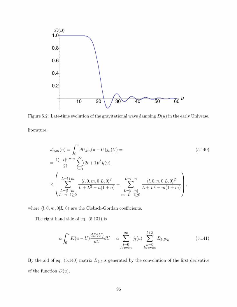
10 20 30 40 50 60u
0.2
0.4
0.6
0.8
1.0
DHuL
Figure 5.2: Late-time evolution of the gravitational wave dampingD(u) in the early Universe.
literature:
Jn,m(u) ≡∫ u
0dUjm(u− U)jn(U) = (5.140)
=4(−i)n+m
2i
∞∑l=0
(2l + 1)iljl(u)
×
L=l+m∑L=|l−m|L−n−1≥0
〈l, 0,m, 0|L, 0〉2L+ L2 − n(1 + n)
+L=l+n∑L=|l−n|m−L−1≥0
〈l, 0, n, 0|L, 0〉2L+ L2 −m(1 +m)
,
where 〈l, 0,m, 0|L, 0〉 are the Clebsch-Gordan coefficients.
The right hand side of eq. (5.131) is
α
∫ u
0K(u− U)
dD(U)
dUdU = α
∞∑l=0
l∈even
jl(u)l+2∑k=0
k∈even
Bk,lck. (5.141)
By the aid of eq. (5.140) matrix Bk,l is generated by the convolution of the first derivative
of the function D(u),
96
D′(u) = (5.142)
=∑n
cn
(jn−3(u)
(−2 + n)n(3 + n)
(−3 + 2n)(−1 + 2n)+ jn−1(u)
n(−3− 4n+ n2
)(−3 + 2n)(3 + 2n)
+jn+1(u)(−1− n)
(2 + 6n+ n2
)(−1 + 2n)(5 + 2n)
+ jn+3(u)(−1− n)(−2 + n)(3 + n)
(3 + 2n)(5 + 2n)
),
with the kernel (5.90) and for integer k ∈ [0, 10] and l ∈ [0, 10] is given by eq. (70) in
Appendix F.
We should notice an unpleasant feature of the matrix of coefficients (70): the first row up
to a factor k = −5 is identical to the second row. This is a direct response to the symmetry
of the introduced function fn(u), eq. (5.178). The functions fn(u) for n = 0 and n = 2 are
exactly the same up to the factor k = −5,
f0(u) = −2
3(j0(u) + j2(u)), (5.143)
f2(u) =10
3(j0(u) + j2(u)).
Therefore the rank of the matrix (70) is Rank[B] = N − 1. This is a real obstacle because
it leads to inconsistency with the boundary conditions. Indeed, the boundary conditions
(5.107) are met if we set
−2
3c0 +
10
3c2 = 1. (5.144)
On the other hand, the linear dependence of the matrix is equivalent to
−2
3c0 +
10
3c2 = 0. (5.145)
97

In order to avoid this unpleasant feature we can start summation in the series (5.136) from
n = 2 instead of n = 0 which is equivalent to setting
c0 ≡ 0, (5.146)
and thus the boundary conditions (5.107) are met if we set
c2 =3
10. (5.147)
Absence of the j2(u) term in the left hand side of eq. (5.137) leads to a restriction on the
first coefficients in eq. (5.141)
−1
3c2 +
4
15c4 = 0. (5.148)
Finally we get the system of linear equations for even integers n ≥ 0,
n(n− 2)(n+ 1)(n+ 3)(2n+ 1)cn = αn+2∑k=0
k∈even
Bk,nck (5.149)
that returns the solution (for even n and k)
cn+2 =
n(n− 2)(n+ 1)(n+ 3)(2n+ 1)cn − α∑n
k=0k∈even
Bk,nck
αBn+2,n. (5.150)
In the limit Q 1 and owing to α ≡ −24fν(0)(4Q)2 we have the Q-independent solution
cn+2 = −
∑nk=0
k∈evenBk,nck
Bn+2,n, (5.151)
98

and therefore for n ∈ [0, 9] we have
c2n =
0,
3
10,3
8,
5
16,
35
128,
63
256,
231
1024,
429
2048,
6435
32768,12155
65536
(5.152)
which completes our series solution (5.136).
5.9 Early-time evolution of the gravitational wave
damping
In this section we rederive the known solution [92] for the graviational wave damping in the
early-time limit, u Q. In this limit eq. (5.106) becomes
u2(d2D(u)
du2+
2
u
dD(u)
du+D(u)
)= β
∫ u
0K(u− U)
dD(U)
dUdU, (5.153)
where
β ≡ −24fν(0). (5.154)
We shall present the analytical solution for eq. (5.153) together with boundary conditions
(5.107). Recalling the differential equation for the spherical Bessel function jn(u),
u2(d2jn(u)
du2+
2
u
djn(u)
du+ jn(u)
)− n(n+ 1)jn(u) = 0, (5.155)
we will look for a solution in terms of a series of spherical Bessel functions
D(u) =∞∑n=0
cnjn(u). (5.156)
99

5 10
5
10
Figure 5.3: Graphical representation for the upper triangular structure of the matrix F2k,2l,eq. (72). The matrix indices l and k define the position of the matrix element in the xy-plane,while along z-axe we plot its value.
The left hand side of eq. (5.153) transforms into
∞∑n=0
n(n+ 1)cnjn(u). (5.157)
The right hand side of eq. (5.153) is represented by the convolution of the kernel (5.90) with
the first derivative of the unknown function D(u) which we are looking for in terms of a
series (5.156).
The right hand side of eq. (5.153) is
β
∞∑l=0
l∈even
jl(u)l∑
k=0k∈even
Fk,lck, (5.158)
where the matrix Fk,l is obtained by the convolution of the kernel (5.90) with the first
100

derivative of the spherical Bessel function,
djn(u)
du=
n
2n+ 1jn−1(u)− n+ 1
2n+ 1jn+1(u), (5.159)
and for integer k ∈ [0, 10] and l ∈ [0, 10] is given in the Appendix G.
Combination of eq. (5.158) and eq. (5.153) leads to the set of linear equations,
n(n+ 1)cn = β
n∑k=0
k∈even
Fk,nck, (5.160)
which returns a convergent solution (for even n and k) [92]
cn =
β∑n−2
k=0k∈even
Fk,nck
n(n+ 1)− βFnn. (5.161)
The boundary conditions (5.107) are met if we set
c0 = 1. (5.162)
The values for the coefficients c2k in the proposed series (5.156) are
c2 =5β
2(−90 + β), (5.163)
c4 =27(−40β + β2
)8(−300 + β)(−90 + β)
,
c6 =13(−756000β − 60960β2 + 469β3
)1680(−630 + β)(−300 + β)(−90 + β)
,
101
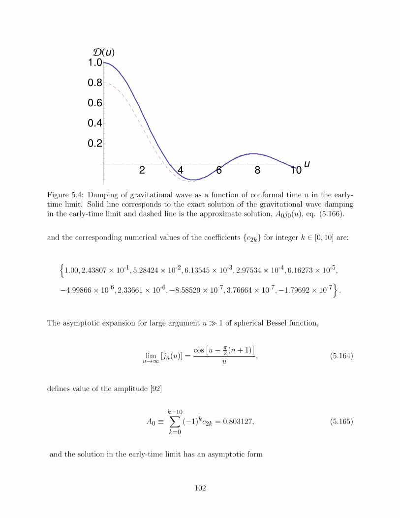
2 4 6 8 10u
0.2
0.4
0.6
0.8
1.0
DHuL
Figure 5.4: Damping of gravitational wave as a function of conformal time u in the early-time limit. Solid line corresponds to the exact solution of the gravitational wave dampingin the early-time limit and dashed line is the approximate solution, A0j0(u), eq. (5.166).
and the corresponding numerical values of the coefficients c2k for integer k ∈ [0, 10] are:
1.00, 2.43807× 10⁻¹, 5.28424× 10⁻², 6.13545× 10⁻³, 2.97534× 10⁻⁴, 6.16273× 10⁻⁵,
−4.99866× 10⁻⁶, 2.33661× 10⁻⁶,−8.58529× 10⁻⁷, 3.76664× 10⁻⁷,−1.79692× 10⁻⁷.
The asymptotic expansion for large argument u 1 of spherical Bessel function,
limu→∞ [jn(u)] =
cos[u− π
2 (n+ 1)]
u, (5.164)
defines value of the amplitude [92]
A0 ≡k=10∑k=0
(−1)kc2k = 0.803127, (5.165)
and the solution in the early-time limit has an asymptotic form
102

D(u) = A0j0(u). (5.166)
Here we have got a numerical value for A0 that differs from S. Weinberg’s [89, 90] value by
about 0.065%. The solution (5.166) is the asymptotic one, which could not be the exact
solution for the problem (5.153). Indeed, the differential operator on the left hand side of
eq. (5.153), being applied to (5.166) returns identical zero, which of course is inconsistent
with the perturbation presented by the right hand side of eq. (5.153). The exact solution is
given by an infinite linear combination of spherical Bessel functions (5.156) with coefficients
(5.164) and asymptotically approaches (5.166). In other words, the perturbation on the
right hand side of eq. (5.153) does not change the behavior of the homogeneous solution eq.
(5.153) but effectively changes the amplitude A0 from unity to the value given by (5.165).
To summarize, the series solution (5.156) with the coefficients (5.164) for the damping
of gravitational wave as a function of conformal time u in the early-time limit is shown in
Fig. 5.4. We note the strict upper triangular structure of matrix F2k,2l that guarantees
the convergent solution for eq. (5.153) in the early-time limit. In this limit the anisotropic
inertia tensor hij(t) never exceeds by absolute magnitude unity and therefore can be treated
as a small perturbation to the metric (5.1). Therefore in the limit u Q the problem
(5.153) leads to damping of a gravitational wave independently of the Q value.
103

5.10 General solution for the gravitational wave
damping
In this section we would like to build the solution for the general gravitational equation
(u(u+ 4Q))2(d2D(u)
du2+
(4(u+ 2Q)
u(u+ 4Q)
)dD(u)
du+D(u)
)(5.167)
= −24fν(0)(4Q)2∫ u
0K(u− U)
dD(U)
dUdU.
Here we define the differential operator
L ≡ (u(u+ 4Q))2(d2
du2+
4(u+ 2Q)
u(u+ 4Q)
d
du+ 1
), (5.168)
and consider the function
fn(u) =n(3 + n)jn−1(u)
4Q+ u+
(−2 + n)(1 + n)jn+1(u)
4Q+ u, (5.169)
then we have equality
L[fn(u)] = 4Q[(−1 + n)n2(3 + n)jn−1(u) + (−2 + n)(1 + n)2(2 + n)jn+1(u)
]+(−2 + n)n(1 + n)(3 + n)(1 + 2n)jn(u). (5.170)
We shall explain the meaning of the obtained eq. (5.170).
First we consider the early-time limit that simplifies the differential operator eq. (5.168)
104

into
limuQ
[L] ≡ L0 = (4Qu)2(d2
du2+
2
u
d
du+ 1
), (5.171)
and the trial function eq. (5.169) reduces to
limuQ
[fn(u)] ≡ f0n(u) =
n(3 + n)
4Qjn−1(u) +
(−2 + n)(1 + n)
4Qjn+1(u). (5.172)
By acting the operator (5.171) on the function (5.172) we obtain
L0[f0n(u)] = (5.173)
= 4Q[(−1 + n)n2(3 + n)jn−1(u) + (−2 + n)(1 + n)2(2 + n)jn+1(u)
]
that exactly coincides with the square brackets (5.170).
Repeating the analogous procedure in the late-time limit, we obtain for the operator
(5.168),
limuQ
[L] ≡ L1 = u4(d2
du2+
4
u
d
du+ 1
), (5.174)
and for the function (5.169),
limuQ
[fn(u)] ≡ f1n(u) =
n(3 + n)jn−1(u)
u+
(−2 + n)(1 + n)jn+1(u)
u
=n(n+ 3)
2n− 1[jn−2(u) + jn(u)] +
(n− 2)(n+ 1)
2n+ 3[jn(u) + jn+2(u)], (5.175)
105

we arrive at the identity
L1[f1n(u)] = (−2 + n)n(1 + n)(3 + n)(1 + 2n)jn(u), (5.176)
that exactly coincides with a single term outside of the square brackets (5.170).
Thus we have proved a nontrivial equality
L[fn(u)] = L0[f0n(u)] + L1[f1
n(u)], (5.177)
which means that action of the general operator L, eq. (5.169), onto the trial function fn(u),
eq. (5.170), returns the exact sum of its action onto the function in the early-time, L0[f0n(u)],
and the late-time, L1[f1n(u)], limits.
As the result of the obtained eq. (5.177) we will be looking for a solution in terms of a
series
D(u) =+∞∑n=0
cn
(n(3 + n)jn−1(u)
4Q+ u+
(−2 + n)(1 + n)jn+1(u)
4Q+ u
). (5.178)
Naturally we have to integrate the right hand side eq. (5.167) for arbitrary n,
−24fν(0)(4Q)2∫ u
0K(u− U)
d
dU
[n(3 + n)jn−1(U)
4Q+ U+
(−2 + n)(1 + n)jn+1(U)
4Q+ U
]dU.
(5.179)
We can break the integral (5.179) into two parts,
∫ u
0−→
∫ u0
0+
∫ u
u0
, (5.180)
106

bearing in mind that u0 Q. This procedure separates the early-time limit, representing
the first integral, from the late-time limit of the second integral
In the early-time limit eq. (5.179) reduces to
−24fν(0)(4Q) (5.181)
×∫ u
0K(u− U)
d
dU[n(3 + n)jn−1(U) + (−2 + n)(1 + n)jn+1(U)] ,
while in the late-time limit it corresponds to
−24fν(0)(4Q)2∫ u
0K(u− U) (5.182)
× d
dU
[n(n+ 3)
2n− 1[jn−2(U) + jn(U)] +
(n− 2)(n+ 1)
2n+ 3[jn(U) + jn+2(U)]
]dU.
Recalling the convolution integral formula (5.140) we will be able to transform the Einstein
field equation (5.167) into a set of linear equations.
After breaking the integral into two parts eq. (5.167) transforms into
+∞∑n=0
cn
[(4Q)
(−1 + n)n2(3 + n)jn−1(u) + (−2 + n)(1 + n)2(2 + n)jn+1(u)
(5.183)
+ (−2 + n)n(1 + n)(3 + n)(1 + 2n)jn(u)] = −24fν(0)(4Q)2
×(
+∞∑n=0
cn
∫ u
0K(u− U)
d
dU
[n(3 + n)jn−1(U) + (−2 + n)(1 + n)jn+1(U)
4Q
]dU
−+∞∑n=0
cn
∫ u
0K(u− U)
× d
dU
[n(n+ 3)
2n− 1[jn−2(U) + jn(U)] +
(n− 2)(n+ 1)
2n+ 3[jn(U) + jn+2(U)]
]dU
).
The early-time limit case that corresponds to the equation formed by the terms inside the
107

curly brackets,
+∞∑n=0
cn
[(−1 + n)n2(3 + n)jn−1(u) + (−2 + n)(1 + n)2(2 + n)jn+1(u)
]= (5.184)
−24fν(0)+∞∑n=0
cn
∫ u
0K(u− U)
d
dU[n(3 + n)jn−1(U) + (−2 + n)(1 + n)jn+1(U)] dU,
exactly reproduces the solution for the early-time evolution of the gravitational wave, and
the late-time limit evolution represented by the differential equation formed by the terms
outside the curly brackets,
+∞∑n=0
cn [(−2 + n)n(1 + n)(3 + n)(1 + 2n)jn(u)] = −24fν(0)(4Q)2 (5.185)
×+∞∑n=0
cn
∫ u
0K(u− U)
× d
dU
[n(n+ 3)
2n− 1[jn−2(U) + jn(U)] +
(n− 2)(n+ 1)
2n+ 3[jn(U) + jn+2(U)]
]dU,
exactly reconstructs the late-time evolution of the gravitational wave.
5.11 Evaluation of the convolution integrals
Here we shall calculate the convolution integrals in the right hand side of eq. (5.183). The
first integral is
−24fν(0)(4Q)+∞∑n=0
cn
∫ u
0K(u− U) (5.186)
× d
dU[n(3 + n)jn−1(U) + (−2 + n)(1 + n)jn+1(U)] dU
= −24fν(0)(4Q)
∞∑l=0
j2l(u)l∑
k=0
A2k+1,2lc2k+1 +∞∑l=0
j2l+1(u)l+1∑k=0
A2k,2l+1c2k
,108
where the matrices A2k+1,2l and A2k,2l+1 are obtained by the convolution of the kernel K(u)
given by eq. (5.90) with the first derivative of the function
d
dU[n(3 + n)jn−1(U) + (−2 + n)(1 + n)jn+1(U)] = (5.187)
= jn−2(U)
((−1 + n)n(3 + n)
−1 + 2n
)+ jn(U)
(−(1 + 2n)
(−2 + 5n+ 5n2
)(−1 + 2n)(3 + 2n)
)+jn+2(U)
(−(−2 + n)(1 + n)(2 + n)
3 + 2n
),
and for integer k ∈ [0, 10] and l ∈ [0, 10] are given in Appendix H.
The second integral that constitutes the right hand side eq. (5.183) is (without the factor
−24fν(0)(4Q)2)
+∞∑n=0
cn
∫ u
0K(u− U) (5.188)
× d
dU
[n(n+ 3)
2n− 1[jn−2(U) + jn(U)] +
(n− 2)(n+ 1)
2n+ 3[jn(U) + jn+2(U)]
]dU
=
∞∑l=0
j2l(u)l+1∑k=0
B2k,2lc2k +∞∑l=0
j2l+1(u)l+1∑k=0
B2k+1,2l+1c2k+1
,where the matrices B2k,2l and B2k+1,2l+1 are obtained by the convolution of the kernel K(u)
(5.90) with the first derivative of the function
d
dU
[n(n+ 3)
2n− 1[jn−2(U) + jn(U)] +
(n− 2)(n+ 1)
2n+ 3[jn(U) + jn+2(U)]
](5.189)
= jn−3(U)
((−2 + n)n(3 + n)
(−3 + 2n)(−1 + 2n)
)+ jn−1(U)
(n(−3− 4n+ n2
)(−3 + 2n)(3 + 2n)
)+
jn+1(U)
(−(1 + n)
(2 + 6n+ n2
)(−1 + 2n)(5 + 2n)
)+ jn+3(U)
(−(−2 + n)(1 + n)(3 + n)
(3 + 2n)(5 + 2n)
),
and for integer k ∈ [0, 10] and l ∈ [0, 10] are given in Appendix F.
109

Finally eq. (5.183) can be written as a set of linear equations
∑n
n(n+ 1)jn(u) (5.190)
× [(4Q)n(n− 3)cn−1 + (n+ 3)(n− 2)(2n+ 1)cn + (4Q)(n+ 1)(n+ 4)cn+1]
= −24fν(0)(4Q)
∞∑l=0
j2l(u)l∑
k=0
A2k+1,2lc2k+1 +∞∑l=0
j2l+1(u)l+1∑k=0
A2k,2l+1c2k
−24fν(0)(4Q)2
∞∑l=0
j2l(u)l+1∑k=0
B2k,2lc2k +∞∑l=0
j2l+1(u)l+1∑k=0
B2k+1,2l+1c2k+1
.Specifying even spherical Bessel functions in eq. (5.190) leads to
2n(1 + 2n) [(4Q)2n(−3 + 2n)c−1+2n + (−2 + 2n)(3 + 2n)(1 + 4n)c2n+ (5.191)
(4Q)(1 + 2n)(4 + 2n)c1+2n] j2n(u)+
+
(24fν(0)(4Q)j2n(u)
n∑k=0
A2k+1,2nc2k+1 + 24fν(0)(4Q)2j2n(u)n+1∑k=0
B2k,2nc2k
)= 0,
which returns the recurrence relation for even coefficients
c2n+2 = − 1
24fν(0)(4Q)2B2n+2,2n× 2n(1 + 2n)[(4Q)2n(−3 + 2n)c−1+2n
+(−2 + 2n)(3 + 2n)(1 + 4n)c2n + (4Q)(1 + 2n)(4 + 2n)c1+2n]+
+
(24fν(0)(4Q)
n∑k=0
A2k+1,2nc2k+1 + 24fν(0)(4Q)2n∑k=0
B2k,2nc2k
). (5.192)
110

Orthogonality between odd spherical Bessel functions in eq. (5.190) returns
(1 + 2n)(2 + 2n) [(4Q)(−2 + 2n)(1 + 2n)c2n+ (5.193)
(−1 + 2n)(4 + 2n)(1 + 2(1 + 2n))c1+2n + (4Q)(2 + 2n)(5 + 2n)c2+2n] j1+2n(u)+
+
(24fν(0)(4Q)j2n+1(u)
n+1∑k=0
A2k,2n+1c2k+
24fν(0)(4Q)2j2n+1(u)n+1∑k=0
B2k+1,2n+1c2k+1
)= 0,
that leads to the recurrence relation for the odd coefficients,
c2n+3 = − 1
24fν(0)(4Q)2B2n+3,2n+1(1 + 2n)(2 + 2n) [(4Q)(−2 + 2n)(1 + 2n)c2n+
+(−1 + 2n)(4 + 2n)(1 + 2(1 + 2n))c1+2n + (4Q)(2 + 2n)(5 + 2n)c2+2n] +
+
(24fν(0)(4Q)
n+1∑k=0
A2k,2n+1c2k + 24fν(0)(4Q)2n∑k=0
B2k+1,2n+1c2k+1
). (5.194)
As we see the coefficients of the general solution depend on the value of the parameter Q.
However, in both early-time and late-time limits the parameter Q 1, and we return to the
Q-independent coefficient values found in the late-time regime, eq. (5.152). Even though
the coefficient ck become Q-independent, the series solution given by (5.178) still depends
on Q-value, and in general is represented by a combination of even and odd spherical Bessel
functions. This is the main conclusion of the general solution of gravitational wave damping
which is in a contradiction with the prediction made by S. Weinberg [89] concerning the
behavior of gravitational wave damping in the early Universe.
111
5.12 Conclusion
We have analyzed the problem of gravitational wave damping in the early Universe due
to freely streaming neutrinos in both early-time and late-time limits. The derivation was
possible with the help of a new compact formula for the convolution of spherical Bessel
functions of integer order.
The exact solution in the early-time limit is given by a convergent series of spherical Bessel
functions of even order with Q-independent coefficients. The neutrino source perturbation
does not change the qualitative behavior of the homogeneous gravitational wave damping
solution but effectively changes its amplitude from unity to the corresponding asymptotic
value.
As in the early-time limit, the late-time limit solution is represented by a convergent
series of spherical Bessel functions of even order and is Q-independent for large values of
Q. Thus the prediction made by S. Weinberg concerning the Q-independent solution for the
gravitational wave damping given by a series of even spherical Bessel functions is valid in
both early-time and late-time limits.
S. Weinberg’s predictions fails in the general case where we were able to construct the
solution in terms of an infinite series of the product of spherical Bessel function and inverse
time parameter u shifted by the value of Q parameter. Even though for large Q-values the
coefficients of the proposed solution are Q-independent, the solution for the gravitational
wave damping depends on Q-value, and in general is represented by a linear combination of
even and odd spherical Bessel functions.
The constructed solution for the general case was possible due the nontrivial equality for
the differential operator of the gravitational wave damping problem which upon its action
112
onto the trial function returns the exact sum of its action onto the function in the early-time
and late-time limits, which we consider as the main result of the present investigation.
Thus we conclude that the problem of gravitational wave damping in the early Universe
due to freely streaming neutrinos is completely solved in an analytical way in both early and
late-time limits, and in the general time case.
113

Chapter 6
Conclusions
In this Thesis we exposed our results in atomic physics, nuclear physics, and cosmology
presented in the quantum scattering language and unified within the framework of the
scattering matrix formalism. Basic governing principles, such as conservation laws and
detailed balance principle, unitarity and gauge invariance of the scattering matrix were
given special attention throughout the Thesis.
In the Atomic Physics chapter we presented the calculation of the axial anomaly
contribution to parity nonconservation (PNC) in atoms. The main result is the prediction
of the emission of an electric photon by the magnetic dipole which has not been observed
yet. The probability of this process is very small but the non-zero result is important from
theoretical point of view.
The Ward identities were imposed on the S-matrix before the calculation of the loop
integral. This allowed us to express the divergent integrals in terms of the convergent ones
and thus obtain the gauge-invariant expression for the S-matrix. We emphasize the vital
difference between the axial anomaly contribution to the PNC effects and the impossibility
for the real Z-boson of spin J = 1 to decay into two real photons, the result known as the
Landau-Yang theorem. The difference is in the virtual photon that connects the triangular
graph of the axial anomaly with the electron atomic transition, e.g., 6s − 7s transition in
cesium, that contributes to the nonzero axial anomaly S-matrix. We have shown that one
can see the impact of the axial anomaly in atomic physics through the parity violation in
114
atoms.
The chapter on Quantum Optics was devoted to the electron laser-assisted scattering
process off an arbitrary central potential. Here we introduced a new method that allowed
us to obtain an analytical cross section for the electron-ion collision in a laser field. For the
illustration of the general method we performed a calculation for the hydrogen laser-assisted
recombination.
The S-matrix of the scattering process was constructed from the electron Coulomb-Volkov
wave function in the combined Coulomb-laser field and the hydrogen perturbed state. By
the aid of the Bessel generating function, the S-matrix was decomposed into an infinite
series of the field harmonics. The new step that resulted in a closed analytical expression
for the cross section of the process was the Plancherel theorem application to the Bessel
generating function. This allowed us to sum the infinite series of Bessel functions and as the
result obtain the cross section of the laser-assisted hydrogen photo-recombination process in
a closed form.
In the Nuclear Physics chapter we investigated the resonance width distribution for low-
energy neutron scattering off heavy nuclei. We used the language of Random Matrix Theory
for describing the nuclear scattering process. Random Matrix Theory that based on the
unitarity of scattering matrix was originally formulated for closed quantum systems. The
unstable complex nucleus is an open quantum system, where the intrinsic dynamics has to
be supplemented by the coupling of chaotic internal states through the continuum. In our
work we proposed a new width distribution based on random matrix theory and the doorway
approach for a chaotic quantum system with a single decay channel. The revealed statistics
of the width distribution exhibits distinctive properties that are characteristically different
from the regularities shared by closed quantum systems. The obtained results directly relate
115

the Porther-Thomas distribution for multiple narrow nuclear resonances to a resonance,
collectivized by the coherent coupling of intrinsic states through the continuum, a nuclear
analog of the Dicke superradiant phenomena in quantum optics.
In the Cosmology chapter our main object of investigation was the space-time metric
perturbed by the stress-energy tensor of neutrino scattering in the early Universe. We have
analyzed the problem of gravitational wave damping in the early Universe due to freely
streaming neutrinos in both early-time and late-time limits.
The Einstein field equation was derived for the traceless and divergenceless tensor
component of the metrics perturbation. The energy-momentum tensor that governs the
neutrino scattering in the early Universe was derived from the kinetic Boltzmann equation. In
the linearized Boltzmann equation neutrinos interact through the metrics perturbation. As
the result, the solution of the Boltzmann equation is given in terms of the tensor component
of the metrics perturbation. Finally we arrived at the intergo-differential Einstein field
equation for the tensor component of the metrics perturbation which we subsequently built
solution for.
The Einstein field equation for the tensor component of the metrics perturbation D(u) is
given in terms of the time parameter u and the dimensionless wavenumber Q. The obtained
equation we analyzed in two extreme cases, the early-time limit, u Q, that corresponds
to the lower-bound wavenumbers q qeq, and the late-time limit, u Q, that is referred
to the upper-bound wavenumbers q qeq. In these cases we were able to build the exact
solution in terms of a convergent series of spherical Bessel functions of even order with Q-
independent coefficients. In the early-time limit, the neutrino source perturbation does not
change the qualitative behavior of the homogeneous gravitational wave damping solution
but effectively changes its amplitude from unity to the corresponding asymptotic value. As
116

in the early-time limit, the late-time limit solution is represented by a convergent series of
spherical Bessel functions of even order and is Q-independent for large values of Q.
Based on the obtained solutions in the extreme cases, we were able to construct the
solution for the general time case due the nontrivial equality for the differential operator
of the gravitational wave damping problem. Its action onto the trial function returns the
exact sum of its action onto the function in the early-time and late-time limits. Even though
for large Q-values the coefficients of the proposed solution are Q-independent, the general
solution for the gravitational wave damping depends on the parameter Q, being represented
by a linear combination of the product of the spherical Bessel function and the inverse sum
of time variable u shifted the parameter Q.
Thus we conclude that the problem of gravitational wave damping in the early Universe
due to freely streaming neutrinos is completely solved in an analytical way in both early and
late-time limits, and in the general time case.
Here we would like to stress that the found property of the general differential operator
is the property of the Einstein field equation for the traceless and divergenceless tensor
component of the metrics perturbation that is independent of the specific form of the energy-
momentum tensor. This means that the developed technique can be equally applied for the
tensor perturbations obtained from the kinetic Boltzmann equation for photons or non-
relativistic matter. We thus hope that the developed method would be helpful for the
corresponding calculations.
117

APPENDICES
118
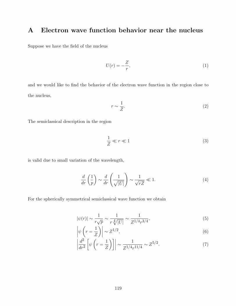
A Electron wave function behavior near the nucleus
Suppose we have the field of the nucleus
U(r) = −Zr, (1)
and we would like to find the behavior of the electron wave function in the region close to
the nucleus,
r ∼ 1
Z. (2)
The semiclassical description in the region
1
Z r 1 (3)
is valid due to small variation of the wavelength,
d
dr
(1
p
)∼ d
dr
(1√|U |
)∼ 1√
rZ 1. (4)
For the spherically symmetrical semiclassical wave function we obtain
|ψ(r)| ∼ 1
r√p∼ 1
r 4√|U |∼ 1
Z1/4r3/4, (5)∣∣∣∣ψ(r =
1
Z
)∣∣∣∣ ∼ Z1/2, (6)∣∣∣∣ d2
dr2
[ψ
(r =
1
Z
)]∣∣∣∣ ∼ 1
Z1/4r11/4∼ Z5/2. (7)
119

Finally the probability to find an electron in the region close to the nucleus in a nonrelativistic
limit is
W ∼ |ψ(r)|2 r3 ∼ 1
Z2. (8)
B Secular equation in the general case
The secular equation for the rotationally invariant Hamiltonian
ε0 − i2η0 h1 h2 h3 h4 · · · hN
h∗1 ε1 − i2η1 v2 v3 v4 · · · vN
h∗2 v∗2 ε2 − i2η2 l3 l4 · · · lN
h∗3 v∗3 l∗3 ε3 0 · · · 0
· · · · · · · · · · · · · · · · · · · · ·
h∗N v∗N l∗N 0 0 · · · εN
(9)
can be written in terms of the matrix
A = (10)
=
h2k
εk−Eα+ Eα − (ε0 − iη0
2 ) h1 −hkvkεk−Eα
h2 −hklkεk−Eα
h1 −hkvkεk−Eα
v2k
εk−Eα+ Eα − (ε1 − iη1
2 ) v2 −vklkεk−Eα
h2 −hklkεk−Eα
v2 −vklkεk−Eα
l2kεk−Eα
+ Eα − (ε2 − iη22 )
,
and is given by
detA = 0. (11)
120

C Friedmann equations
In this Appendix we give a detailed derivation of the fundamental Friedmann equation.
We start from the Ricci tensor that in components looks like,
Rij =∂Γkki∂xj
−[∂Γkij
∂xk+∂Γ0
ki
∂t
]+[Γ0ikΓkj0 + Γki0Γ0
jk + ΓlikΓkjl
]−[ΓkijΓ
lkl + Γ0
ijΓl0l
], (12)
R00 =∂Γii0∂t
+ Γi0jΓj0i. (13)
First we separate the spatial-spatial part of the Ricci tensor, Rij ,
Rij =∂Γkki∂xj
−∂Γkij
∂xk+ ΓlikΓkjl − ΓkijΓ
lkl. (14)
On the other hand the spatial part of the spherically symmetric and isotropic metrics is
given by
gij = δij +Kxixj
1−Kx2, (15)
gij∣∣x=0 = δij , (16)
where K is the curvature constant. We note that the spatial components of the 4D affine
connections Γkij are proportional to the affine connection calculated in the 3D from the spatial
part of the metric tensor gij ,
Γkij = Kxkgij . (17)
121

Further we calculate the spatial Ricci tensor at x = 0,
Rij
∣∣∣x=0
=∂Γkki∂xj
−∂Γkij
∂xk= Kδij − 3Kδij = −2Kδij . (18)
Recalling the metrics (15) we reconstruct the spatial Ricci tensor for every point,
Rij = −2Kgij , (19)
which is valid for all spatial coordinate systems.
The space-time components of the affine connections appearing in the Ricci tensor,
∂Γ0ij
∂t= gij
d
dt(aa), (20)
∂Γii0∂t
= 3d
dt
(a
a
),
Γ0ikΓkj0 = gij a
2,
Γ0ijΓ
l0l = 3gij a
2,
Γi0jΓji0 = 3
(a
a
)2
.
As the result, we have for the Ricci tensor,
Rij = Rij −[gij
d
dt(aa)
]+[2gij a
2]−[3gij a
2]
(21)
= Rij − 2a2gij − aagij ,
R00 = 3d
dt
(a
a
)+ 3
(a
a
)2
= 3a
a. (22)
Recalling the space-space components of the Ricci tensor eq. (18), we arrive at the final
122
expression for the Ricci tensor,
Rij = −[2K + 2a2 + aa
]gij . (23)
The energy-momentum tensor is given in terms of energy density ρ and pressure p,
T00 = ρ, (24)
Ti0 = T0i = 0,
Tij = a2pgij .
Therefore the shifted energy-momentum tensor Sµν ,
Sµν = Tµν −1
2gµνT
λλ, (25)
in components looks like
Sij = Tij −1
2gija
2Tλλ = a2pgij −1
2gija
2(3p− ρ) =1
2(ρ− p)a2gij , (26)
S00 = T00 +1
2Tλλ = ρ+
1
2(3p− ρ) =
1
2(3p+ ρ). (27)
Finally the Einstein equations are,
−[2K + 2a2 + aa
]gij = −4πG(ρ− p)a2gij , (28)
3a
a= −4πG(3p+ ρ). (29)
123

Simple algebra leads to the fundamental Friedmann equations,
ρ =3
8πG
(a2
a2+K
a2
), (30)
p = − 1
8πG
(2a
a+a2
a2+K
a2
), (31)
In the case when we can neglect the curvature constant termK, Friedmann equations simplify
to
ρ =3
8πG
(a2
a2
)=
3
8πGH2, (32)
p = − 1
8πG
(2a
a+a2
a2
). (33)
D Energy density for fermions and bosons in the early
Universe
We start form the number density n(p) for fermions, n+f (p, T ), and bosons, n−b(p, T ), with
the rest mass m, momentum p, with number of spin states, or the number of independent
polarization states g,
n±(p, T ) = g4πp2
(2πh)3
1
exp
[√p2+m2
kT
]± 1
. (34)
124

The energy, pressure and entropy density are given in terms of the number density n(p) by
ρ(T ) =
∫ ∞0
dp n(p, T )
√p2 +m2, (35)
p(T ) =
∫ ∞0
dp n(p, T )p2
3√p2 +m2
, (36)
s(T ) =1
T
∫ ∞0
dp n(p, T )
(√p2 +m2 +
p2
3√p2 +m2
). (37)
For massless particles we obtain
ρ±(T ) =
∫ ∞0
dp g4πp3
(2πh)3
1
exp[ pkT
]± 1
. (38)
In order to perform the momentum integration in eq. (38) we employ the standard integrals,
∫ ∞0
z2n−1
ez + 1=
22n−1 − 1
2nπ2nBn, (39)∫ ∞
0
z2n−1
ez − 1=
(2π)2n
4nπ2nBn, (40)
given in terms of the Bernoulli numbers Bn. Thus we obtain the massless fermion and boson
contribution to the energy density,
ρ−(T ) =g
2aBT
4, (41)
ρ+(T ) =7g
16aBT
4 =7
8ρ−(T ) (42)
where we used the earlier introduced notation,
aB =4σ
c=
8π5k4
15(2πhc)3. (43)
125

For the entropy density of photons, electrons and positrons,
s(T ) =4
3aBT
3 (44)
+2× 2
T
∫ ∞0
dp4πp2
(2πh)3
1
exp
[√p2+m2
ekT
]+ 1
(√p2 +m2
e +p2
3√p2 +m2
e
).
In terms of the dimensionless parameter,
x =me
kT, (45)
the entropy density (44) is given in terms of the function F (x).
F (x) = (46)
= 1 +45
2π4
∫ ∞0
dy y2 1
exp[√
y2 + x2]
+ 1
(√y2 + x2 +
y2
3√y2 + x2
),
with its asymptotic behavior,
F (0) =11
4, (47)
limx→∞F (x) = 1. (48)
As the result, the contribution of photons, electrons and positrons to the entropy density is,
s(T ) =4
3aBT
3F(me
kT
)(49)
126

The condition of thermal equilibrium can be expressed in term of entropy as,
s(T )a3 = const. (50)
Applying the thermal equilibrium condition in the limit that corresponds to the neutrino
temperature, kTν me, and to the photon temperature, kT me, we get,
Tν = T
(F (me/kT )
F (me/kTν)
)1/3
= T
(11
4
)−1/3
. (51)
Finally the photon, neutrino, and antineutrino contribution to the energy density is,
ρ(T ) = aBT4 +
(3× 2× 7
16
)aBT
4ν = aBT
4 + aBT4(
3× 2× 7
16
)(4
11
)4/3
. (52)
As the result, we obtain the ratio of neutrino energy density to the total neutrino and photon
energy density,
fν(0) =ρν
ργ + ρν=
3(
78
)(411
)4/3
1 + 3(
78
)(411
)4/3' 0.40523. (53)
E Convolution integral of spherical Bessel functions
Here we derive the convolution integral (5.140) of spherical Bessel functions for integer orders
n,m. Theoretical efforts for such a convolution integral were put forward in [92] but here
we report a new compact formula that has a clear exchange symmetry (n←→m) and can be
readily applied for practical calculations.
127

Starting with the integral
Jn,m(u) ≡∫ u
0dUjm(u− U)jn(U), (54)
we prove eq. (5.140). First, we represent a spherical Bessel function as a Fourier
transformation of the Legendre polynomial Pn(z),
jn(u) =(−i)n
2
∫ 1
−1ds exp(ius)Pn(s). (55)
Substitution of (55) into (54) leads to
Jn,m(u) =(−i)n+m
4
∫ 1
−1ds
∫ 1
−1dt exp(iut)Pm(s)Pn(t)
∫ u
0dU exp(iUs− iUt)
=(−i)n+m
4i
∫ 1
−1ds
∫ 1
−1dtPm(s)Pn(t)
exp(ius)− exp(iut)
(s− t) . (56)
Now we employ the Legendre function of the second kind Qn(z) defined as
Qn(z) =1
2
∫ 1
−1dz′
Pn(z′)z − z′ . (57)
Performing the integrations over t and s we obtain
(−i)n+m
4i
∫ 1
−1ds
∫ 1
−1dtPm(s)Pn(t)
exp(ius)− exp(iut)
(s− t) (58)
=(−i)n+m
2i
∫ 1
−1dt exp(iut) [Pn(t)Qm(t) + Pm(t)Qn(t)] .
Further we reincarnate spherical Bessel functions by decomposing plane waves in terms of
128

Legendre polynomials
exp(iut) =∞∑l=0
(2l + 1)iljl(u)Pl(t), (59)
which leads to
(−i)n+m
2i
∫ 1
−1dt exp(iut) [Pn(t)Qm(t) + Pm(t)Qn(t)] (60)
=(−i)n+m
2i
∞∑l=0
(2l + 1)iljl(u)
∫ 1
−1dtPl(t) [Pn(t)Qm(t) + Pm(t)Qn(t)] .
The angular momentum coupling simplifies the product of Legendre polynomials,
Pl(x)Pm(x) =L=l+m∑L=|l−m|
〈l, 0,m, 0|L, 0〉2PL(x), (61)
in terms of the Clebsch - Gordan coefficients 〈l, 0,m, 0|L, 0〉. Introducing
Wm−1(z) = 2
[m−12 ]∑
k=0
(m− 2k − 1)
(2k + 1)(m− k)Pm−2k−1(z), (62)
and using the analog of eq. (61),
Pl(z)Qm(z) =L=l+m∑L=|l−m|
〈l, 0,m, 0|L, 0〉2 (QL(z) +WL−1(z))− Pl(z)Wm−1(z), (63)
129

we come to
∫ 1
−1dtPl(t) [Pn(t)Qm(t) + Pm(t)Qn(t)] (64)
=
∫ 1
−1dt
Pn(t)Pl(t)Qm(t)︸ ︷︷ ︸I
+Pl(t)Pm(t)︸ ︷︷ ︸II
Qn(t)
=
∫ 1
−1dt
Pn(t)
L=l+m∑L=|l−m|
〈l, 0,m, 0|L, 0〉2 (QL(t) +WL−1(t))− Pl(t)Wm−1(t)
+
L=l+m∑L=|l−m|
〈l, 0,m, 0|L, 0〉2PL(t)Qn(t)
,where in the first term we have decomposed the product Pl(t)Qm(t), whereas in the second
term we decomposed the product Pl(t)Pm(t). Using the parity identity,
∫ 1
−1dtPn(t)QL(t) = −
∫ 1
−1dtPL(t)Qn(t), (65)
we obtain
∫ 1
−1dtPl(t) [Pn(t)Qm(t) + Pm(t)Qn(t)] (66)
=
∫ 1
−1dt
Pn(t)
L=l+m∑L=|l−m|
〈l, 0,m, 0|L, 0〉2WL−1(t)− Pl(t)Wm−1(t)
.
130

Therefore
∫ 1
−1dt
L=l+m∑L=|l−m|
〈l, 0,m, 0|L, 0〉2Pn(t)WL−1(t) (67)
=
∫ 1
−1dt
L=l+m∑L=|l−m|
〈l, 0,m, 0|L, 0〉2[(L−1)/2]∑k=0
2L− 4k − 1
(2k + 1)(L− k)PL−2k−1(t)Pn(t)
= 4L=l+m∑L=|l−m|L−n−1≥0
〈l, 0,m, 0|L, 0〉2L+ L2 − n(1 + n)
.
On the other hand,
∫ 1
−1dtPl(t)Wm−1(t)Pn(t) (68)
=
∫ 1
−1dt
[(m−1)/2]∑k=0
2m− 4k − 1
(2k + 1)(m− k)Pm−2k−1(t)Pl(t)Pn(t)
=
∫ 1
−1dt
[(m−1)/2]∑k=0
2m− 4k − 1
(2k + 1)(m− k)Pm−2k−1(t)
L=l+n∑L=|l−n|
〈l, 0, n, 0|L, 0〉2PL(t)
= −4L=l+n∑L=|l−n|m−L−1≥0
〈l, 0, n, 0|L, 0〉2L+ L2 −m(1 +m)
.
Thus, the identity (5.140) is demonstrated,
∫ 1
−1dt
L=l+m∑L=|l−m|
〈l, 0,m, 0|L, 0〉2Pn(t)WL−1(t)−∫ 1
−1dtPn(t)Pl(t)Wm−1(t)
= 4L=l+m∑L=|l−m|L−n−1≥0
〈l, 0,m, 0|L, 0〉2L+ L2 − n(1 + n)
+ 4L=l+n∑L=|l−n|m−L−1≥0
〈l, 0, n, 0|L, 0〉2L+ L2 −m(1 +m)
. (69)
131

5 10
5
10
Figure 1: Graphical representation for the upper but one triangular structure of the matrixB2k,2l. The matrix indices l and k define a position of the matrix element in the xy-plane,while along z-axe we plot its value.
F Convolution matrices in the late-time limit
B2k,2l ≡ (70)
0 115
110
13350
174900 − 1
37801
19404 − 291981980
1193050
0 −13 −1
2 −1370 − 17
9801
756 − 519404
29396396 − 1
38610
0 415
755 − 5671
17325 −1052344100 − 733
13860 − 1453640332 − 29
77297220173
5855850
0 0 1855
7933465 −3013
8820 −1350741580 − 2077
23716 − 1247220220
3531351350
0 0 0 88225
68323209475 − 6611
17955 −13433234 − 3652637
30060030 − 4375681491891400
0 0 0 0 2657
16613933 − 81703
204930 −45208398918910 − 39881
257400
0 0 0 0 0 1223
74315143451 −244553
567567 −302161504504
0 0 0 0 0 0 238405
7010171142505 −2355893
5077800
0 0 0 0 0 0 0 304465
1153916275
132

5 10
5
10
Figure 2: Graphical representation for the upper but one triangular structure of the matrixB2k+1,2l+1. The matrix indices l and k define a position of the matrix element in thexy-plane, while along z-axe we plot its value.
B2k+1,2l+1 ≡ (71)
625 −17
75 −1170 − 23
147095
15876 − 55434365900
1046323123100 − 713
356756428343
281582730
625
47675 − 91
270 −127630 − 19
540 − 161326700 − 439
3303300589
11042460 − 203993860910
0 827
4402457 − 9509
28665 − 742926460 − 102373
1455300 − 99132484300
5894471740
51085994
0 0 1439
12894641 −13655
38556 − 5074491372140 − 898553
8588580 − 2368307324648324
152875394215822
0 0 0 3685
400910710 − 6638
17325 −126901275275 − 4156573
30060030 − 61151558402344
0 0 0 0 2245
5291125 − 9433
22750 −116219210210 − 4553149
26546520
0 0 0 0 0 208375
1435825375 −1907
4263 − 921114280
0 0 0 0 0 0 1829
93031140679 −226529
471240
0 0 0 0 0 0 0 6899
1108714652
133

5 10
5
10
Figure 3: Graphical representation for the upper triangular structure of the matrix F2k,2l, eq.(72). The matrix indices l and k define the position of the matrix element in the xy-plane,while along z-axe we plot its value.
G Convolution matrix in the early-time limit
F2k,2l ≡ (72)
0 −16 − 1
10 − 13900
1711025 − 1
252025
174636 − 29463320
132175
0 115 − 1
20 − 13315 − 17
25201
1260 − 14536
29343035 − 1
25740
0 0 115 − 143
3150 − 2216300 − 41
756085
137214 − 5513243240
1632509650
0 0 0 115 − 17
392 − 17525 − 18715
38419928207
15057900 − 23156156
0 0 0 0 115 − 19
450 − 5162 − 2850091
62432370059
117117
0 0 0 0 0 115 − 115
2772 − 1454851 − 12247
2802800
0 0 0 0 0 0 115 − 261
6370 − 31910920
0 0 0 0 0 0 0 115 − 341
8400
0 0 0 0 0 0 0 0 115
134
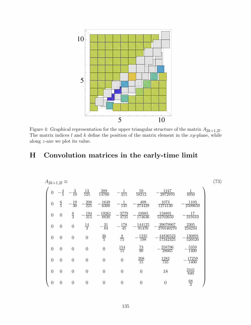
5 10
5
10
Figure 4: Graphical representation for the upper triangular structure of the matrix A2k+1,2l.The matrix indices l and k define the position of the matrix element in the xy-plane, whilealong z-axe we plot its value.
H Convolution matrices in the early-time limit
A2k+1,2l ≡ (73)
0 −45 − 3
1013525
28914700 − 1
31559
58212 − 12472972970
14950
0 65 −19
30 −208225 −1649
6300 − 1135 − 409
2744281073
1274130 − 11032509650
0 0 83 −194
315 −192618820 −3779
4725 − 10985174636
15889152702650 − 17
319410
0 0 0 143 −31
84 −17845 −144125
91476 − 39079907270540270
2305234234
0 0 0 0 365
875 −1235
198 −4483652317342325 −130891
520520
0 0 0 0 0 15415
7390 −258796
28665 −53591400
0 0 0 0 0 0 20815
1282735 −17259
1400
0 0 0 0 0 0 0 18 2441840
0 0 0 0 0 0 0 0 683
135

5 10
5
10
Figure 5: Graphical representation for the upper triangular structure of the matrix A2k,2l+1.The matrix indices l and k define the position of the matrix element in the xy-plane, whilealong z-axe we plot its value.
A2k,2l+1 ≡ (74)
− 215
19
22225
5294 − 19
945023
41580 − 29555
31326700 − 35
722007
23 −5
9 −2245 − 25
29419
1890 − 238316
21911 − 31
65340175
722007
0 2815 −49
75 −7349 −1577
3150 − 4853152460
177385385
858718404100 − 1069
3128697
0 0 185 −383
735 −56811890 −882947
762300 − 5807965780775
4061660660 − 509
722007
0 0 0 8815 −151
945 −8719317325 −154003
75075 − 585549730060030
21778715459444
0 0 0 0 263
71165 −492
65 −13457142350 − 33633
106964
0 0 0 0 0 12 341273 −4681
441 −25262555692
0 0 0 0 0 0 23815
36171575 −8671
612
0 0 0 0 0 0 0 30415
911255
136

BIBLIOGRAPHY
137

BIBLIOGRAPHY
[1] M. A. Bouchiat and C. C. Bouchiat, Physics Letters B, 48, 111 (1974).
[2] C. S. Wood, S. C. Bennet, D. Cho, B. P. Masterson, J. L. Roberts, C. E. Tanner andC. E. Wieman, Science 275, 1759 (1997).
[3] A. Schafer, G. Soff, P. Indelicato, B. Muller, and W. Greiner, Phys. Rev. A 40, 7362(1989).
[4] R. W. Dunford, Phys. Rev. A 54, 3820 (1996).
[5] L. N. Labzowsky, A. V. Nefiodov, G. Plunien, G. Soff, R. Marrus and D. Liesen, Phys.Rev. A 63, 054105 (2001).
[6] M. Zolotorev and D. Budker, Phys. Rev. Lett. 78, 4717 (1997).
[7] M. Y. Kuchiev and V. V. Flambaum, Phys. Rev. Lett. 89, 283002 (2002).
[8] A. I. Milstein, O. P. Sushkov and I. S. Terekhov, Phys. Rev. Lett. 89, 283003 (2002).
[9] V. M. Shabaev, K. Pachucki, I. I. Tupitsyn and V. A. Yerokhin, Phys. Rev. Lett. 94,213002 (2005).
[10] V. V. Flambaum and J. S. M. Ginges, Phys. Rev. A 72 , 052115 (2005).
[11] J. Sapirstein, K. Pachucki, A. Vietta and K. T. Cheng, Phys. Rev. A 67, 052110 (2003).
[12] I. Bednyakov, L. Labzowsky, G. Plunien, G. Soff and V. Karasiev, Phys. Rev. A 61,012103 (1999).
[13] S. Weinberg, The Quantum Theory of Fields, Vol. 2. Modern Applications (CambridgeUniversity Press, Cambridge, UK, 2000).
[14] S. Adler, Phys. Rev. 177, 2426 (1969);J. S.Bell and R. Jackiw, Nuovo Cimento A 60, 47, (1969).
138
[15] I. B. Khriplovich, Parity Noncoservation in Atomic Phenomena (Gordon and Breach,London, 1991).
[16] L. Rosenberg, Phys. Rev. 129, 2786 (1963); M.L. Laursen and M.A. Samuel, Z. Phys.C 14, 325 (1982); A. Barroso et al., Z. Phys. C 28, 149 (1985).
[17] L. D. Landau, Dokl. Akad. Nauk. S.S.S.R. 60, 207 (1948);C.N.Yang Phys. Rev. 77, 242 (1950).
[18] A. I. Akhiezer and V. B. Berestetskii, Quantum Electrodynamics (IntersciencePublishers, New York, 1965).
[19] C. Itzykson and J.B. Zuber, Quantum Field Theory (McGraw-Hill, 1980).
[20] L. D Landau and E. M. Lifschitz, Quantum Mechanics Non-Relativistic Theory (Oxford,Pergamon Press, 1977).
[21] M. H. Mittleman, Introduction to the Theory of Laser-Atom Interactions (New York,Plenum Press, 1993); C. J. Joachain, Laser Interaction with Atoms, Solids and Plasmas(New York, Plenum Press, 1994).
[22] G. Gabrielse et al, ATRAP collaboration, Phys. Rev. Lett, 89, 213401 (2002);M. Amoretti et al, ATHENA Collaboration, Nature, 419, 456 (2002).
[23] G. Gabrielse et al., http//cdsweb.cern.ch/record/1234581/files/CERN-SPSC-2010-006.
[24] M. Amoretti et al., ATHENA Collaboration, Phys. Rev. Lett. 97 213401;G. Gabrielse et al., ATRAP collaboration, Phys. Rev. Lett. 100, 113001 (2008).
[25] T. Pohl, D. Vrinceanu, and H. R. Sadeghpour, Phys. Rev. Lett. 100, 223201 (2008).
[26] F. Robicheaux, Phys. Rev. A 70, 022510 (2004); S. Roy, S. Ghosh, and C. Sinha Phys.Rev. A 78, 022706 (2008).
[27] G. Gabrielse, Adv. At., Mol., Opt. Phys. 50, 155 (2005).
[28] H. R. Reiss, Phys. Rev. A 22, 1786 (1980); F. W. Byron, P. Francken, and C. J.Joachain, J. Phys. B 20, 5487 (1987); P. Franken, C. J. Joachain, Phys. Rev. A 35,1590 (1987); P. Franken, C. J. Joachain, J. Opt. Soc. Am. B 7, 554 (1990).
139

[29] L. Shu-Min, C. Ji , Z. Jian-Ge, and Y. Hong-Jun, Phys. Rev. A 47 1197 (1993); L. Shu-Min, M. Yan-Gang, Z. Zi-Fang, C. Ji,and L. Yao-Yang,Phys. Rev. A 58 2615 (1998).
[30] M. Stobbe, Ann. Phys. 7, 661 (1930).
[31] M. Jain and N. Tzoar, Phys. Rev. A 18, 538 (1978).
[32] A. I. Akhiezer and N. P. Merenkov, J. Phys. B 29, 2135 (1996).
[33] W. Rudin, Principles of Mathematical Analysis (New York McGraw-Hill, 1976).
[34] G. Bateman and A. Erdelyi, Higher Transcendental Functions (New York McGraw-Hill,1953); I. S. Gradshteyn and I. M. Ryzhik, Table of Integrals, Series and Products (NewYork Academic Press, 1965).
[35] L. V. Keldysh, Sov. Phys. JETP 20, 1307 (1965).
[36] K. C. Kulander, Phys. Rev. A 35, 445 (1987);J. L. Krause, K. J. Schafer, and K. C. Kulander, Phys. Rev. A 45, 4998 (1992).
[37] M.L. Mehta, Random Matrices, 3rd ed., (Elsevier, Amsterdam, 2004).
[38] A. Bohr and B.R. Mottelson, Nuclear Structure (World Scientific, Singapore, 1998).
[39] V. Zelevinsky, B.A. Brown, N. Frazier, and M. Horoi, Phys. Rep. 276, 85 (1996).
[40] H.-J. Stockmann, Quantum chaos an introduction (Cambridge University Press, 2000).
[41] H.A. Weidenmuller and G.E. Mitchell, Rev. Mod. Phys. 81, 539 (2009).
[42] T.A. Brody, J. Flores, J.B. French, P.A. Mello, A. Pandey, and S.S.M. Wong, Rev. Mod.Phys. 53, 385 (1981).
[43] C.E. Porter and R.G. Thomas, Phys. Rev. 104, 483 (1956).
[44] P. E. Koehler, F. Becvar, M. Krticka, J. A. Harvey, and K. H. Guber, Phys. Rev. Lett.105, 072502 (2010).
[45] P.E. Koehler, Phys. Rev. C 84, 034312 (2011).
140

[46] H.-J. Sommers, Y.V. Fyodorov and M. Titov, J. Phys. A 32, L77 (1999).
[47] U. Kuhl, R. Hohmann, J. Main, and H.-J. Stockmann, Phys. Rev. Lett. 100, 254101(2008).
[48] Y. Fyodorov and H.-J. Sommers, J. Math. Phys. 38, 1918 (1997).
[49] D.V. Savin and V.V. Sokolov, Phys. Rev. E 56, R4911 (1997).
[50] H.A. Weidenmuller, Phys. Rev. Lett. 105, 232501 (2010).
[51] G.L. Celardo, N. Auerbach, F.M. Izrailev and V.G. Zelevinsky, Phys. Rev. Lett. 106,042501 (2011).
[52] A. Volya, Phys. Rev. C 83, 044312 (2011).
[53] G.E. Mitchell, J.D. Bowman, S.I. Penttil, and E.I. Sharapov, Phys. Rep. 354, 157(2001).
[54] V.V. Flambaum and V.G. Zelevinsky, Phys. Lett. B 350, 8 (1995).
[55] V.V. Sokolov and V.G. Zelevinsky, Nucl. Phys. A504, 562 (1989).
[56] C. Mahaux and H.A. Weidenmuller, Shell Model Approach to Nuclear Reactions (NorthHolland, Amsterdam, 1969).
[57] N. Auerbach and V. Zelevinsky, Rep. Prog. Phys. 74, 106301 (2011).
[58] S. Mizutori and V. Zelevinsky, Z. Phys. A346, 1 (1993).
[59] A. M. Lane and R. G. Thomas, Rev. Mod. Phys. 30, 257 (1958).
[60] N. M. Larson, Oak Ridge National Laboratory Technical Report No. ORNL/TM-9179/R8, (2008).
[61] V.V. Sokolov and V.G. Zelevinsky, Ann. Phys. 216, 323 (1992).
[62] N. Auerbach and V. Zelevinsky, Nucl. Phys. A781, 67 (2007).
141

[63] P. von Brentano, Phys. Rep. 264, 57 (1996).
[64] H. Komano, M. Igashira, M. Shimizu, and H. Kitazawa, Phys. Rev. C 29, 345 (1984).
[65] G.L. Celardo, A.M. Smith, S. Sorathia, V.G. Zelevinsky, R.A. Sen’kov, and L. Kaplan,Phys. Rev. B 82, 165437 (2010).
[66] J. Flores et al., AIP Conf. Proc. 1323, 62 (2010).
[67] A. A. Starobinsky, JETP Lett. 30, 682 (1979); Phys. Lett. B91, 99 (1980).
[68] D. Kazanas, Astrophys. J. 241, L59 (1980).
[69] K. Sato, Mon. Not. Roy. Astron. Soc. 195, 467 (1981).
[70] A. Guth, Phys. Rev. D 23, 347 (1981).
[71] A. D. Linde, Phys. Lett. B108, 389 (1982); 114, 431 (1982); Phys. Rev. Lett. 48, 335(1982).
[72] A. Albrecht and P. Steinhardt, Phys. Rev. Lett. 48, 1220 (1982).
[73] S. V. Mukhanov and G. V. Chibisov, Sov. Phys. JETP Lett. 33, 532 (1981).
[74] S. Hawking, Phys. Lett. 115B, 295 (1982).
[75] A. A. Starobinsky, Phys. Lett. 117B, 175 (1982).
[76] A. Guth and S.-Y. Pi, Phys. Rev. Lett. 49, 1110 (1982); Phys. Rev. D 32, 1899 (1985)
[77] J. M. Bardeen, P. J. Steinhardt, and M. S. Turner, Phys. Rev. D 28, 679 (1983).
[78] W. Fischler, B. Ratra, and L. Susskind, Nucl. Phys. B 259, 730 (1985).
[79] N. Seto, S. Kawamura, and T. Nakamura, Phys. Rev. Lett. 87, 221103 (2001).
[80] T. L. Smith, M. Kamionkowski, and A. Cooray, Phys. Rev. D 73, 023504 (2006).
[81] G. Efstathiou and S. Chongchitnan, Prog. Theor. Phys. Suppl. 163, 204 (2006).
142
[82] B. Friedman, A. Cooray, and A. Melchiorri, Phys. Rev. D 74, 123509 (2006).
[83] http//www.map.gsfc.nasa.gov
[84] E. Komatsu et al., Astrophys. J. Suppl. 180, 330 (2009); 192, 18 (2011).
[85] D. N. Spergel et al., Astrophys. J. Suppl. 148, 175 (2003); 170, 377 (2007).
[86] C. L. Bennett et al., Astrophys. J. Suppl. 148, 1 (2003).
[87] http//www.ligo.caltech.edu
[88] J. Abadie et al., Phys. Rev. Lett. 107, 271102 (2011);Nature Physics 7, 962 (2011); Phys. Rev. D 85, 022001 (2012).
[89] S. Weinberg, Cosmology, (Oxford University Press, 2008).
[90] S. Weinberg, Phys. Rev. D 69, 023503 (2004).
[91] S. Weinberg, Phys. Rev. D 74, 063517 (2006).
[92] D. A. Dicus and W. W. Repko, Phys. Rev. D 72, 088302 (2005).
[93] J. M. Stewart, Astrophys. J. 176, 323 (1972).
[94] E. T. Vishniac, Astrophys. J. 257, 456 (1982).
[95] J. R. Bond and A. S. Szalay, Astrophys. J. 274, 443 (1983).
[96] M. Kasai and K. Tomita, Phys. Rev. D 33, 1576 (1986).
[97] A. K. Rebhan and D. J. Schwarz, Phys. Rev. D 50, 2541 (1994).
[98] J. R. Pritchard and M. Kamionkowski, Ann. Phys. (N.Y.) 318, 2 (2005).
[99] Y. Watanabe and E. Komatsu, Phys. Rev. D 73, 123515 (2006).
143