SCANNER DATA: TOWARDS CONSTANT

UTILITY INDEXES?

Patrick SILLARD(*)

(*)INSEE, Division des prix a la consommation

Introduction

Price indices are now well internationally defined economic indicators. In particular, themethods applied by European countries are made comparable. Price indices are constant-quality indices. In other words, the price index aims at reflecting the evolution of theprices of goods, the level of quality being fixed. From the economic point of view, theunderlying concept is the utility constant price index (see for example [21, 27]). But,unless we adopt very restrictive assumptions, constant quality indexes are not coincidentwith constant utility indexes. Indeed, the constant utility framework supposes to observethe substitution that occurs between the consumption of goods during the successivestates of the economy. In other words, if one wants to build constant utility indexes inthe general case, one need to observe demand functions.

From the microeconomic point of view, substitutions concern goods of the same type,sold within a geographically limited area where the substitution is practically possible forthe consumer. The question of how far are constant utility indexes from constant qualityindices arises only at the level of micro-aggregates, that is the elementary computationof a price index based on the prices themselves. After this computation, the elementaryaggregates are combined through a Laspeyres aggregation in a separate operation. Thispaper only deals with micro-aggregates.

Practically, the joint observation of selling prices and quantities supposes the avail-ability of scanner data. In the project carried out by Insee, some retailors allowed Inseeto have access to their scanner data. The whole data sets covers 3 years for 1000 shopsand 10 families of products.

The bias of price indices has been a central issue of the Boskin Commission in the late1990s [3, 23, 7] in the US. This work has shown the distance between classical indexes andconstant utility indexes (Cost of Living Index). They also showed that the observationof demand functions makes it possible to build constant utility indexes. Some studieshave been made on price index biases, especially those ones linked with introductionof new goods or loss of existing goods [14]. The empirical application of these ideasis stayed limited until the availability of scanner data. The papers on scanner data aremainly related to substitution phenomenons [9, 15, 17]. The present paper examines morespecifically the application of these ideas to price indices.

1

1 The economic framework of consumer price indices

The breakdown of good consumption into volumes and prices is a fundamental issue forprice indices. The empirical approach that prevails in most modern price indices, however,rests on a number of assumptions that can be reviewed within the theoretical frameworkof microeconomic theory of consumer behavior [5].

1.1 Economic modelling

We postulate, consistently with microeconomic theory [25], that the consumer makeschoices among all the baskets of goods he may consume. He takes his decision accordingto a utility function maximised under a budget constraint.

Let us denote by p the price vector and s that of quantities, u the representative con-sumer utility function (the function is supposed to be time-independent). The consumerdecides to consume a quantity vector x based on the following optimization program(whose argument is x) :

e(p, U) =

∣∣∣∣∣ mins

p.s

u.c. u(s) = U(1)

Like this, e(p, U) is the expenditure function : it is the minimum amount of moneythe consumer must do to reach the utility level U conditionally to the exogenous pricevector p. In a dual manner, the maximum of utility that it is possible to reach for agiven spending R conditionally to the exogenous price vector p is the indirect utility. Wedenote this function by v(p, R).

Let us consider now to different times: a reference one t and a second one t′ (t′ > t).Between the two periods of time, we want to build a price index that shows the evolutionof prices. The observables are prices at both times and the initial spending Rt. At t, theconsumer-optimiser reaches a utility level v(pt, Rt). In order to reach the same utilitylevel at t′, he must spend e(pt′ , v(pt, Rt)). By construction, the constant utility priceindex is :

I t′,tCU(Rt) =

e(pt′ , v(pt, Rt))

Rt

(2)

This reflects changes in the budget that the consumer must accept to maintain itsutility at t′ at the level he reached at t with a spending Rt. It useful at this stage todefine the first argument of the previous ratio (p and q are two price vectors ; R is anyexpense) :

µ(p; q, R) = e(p, v(q, R)) (3)

This function is the money metric indirect utility function. It corresponds to the spendingthe consumer must do, at price p, to reach the utility level that he reaches with the pricevector q and a spending R.

With the help of the money metric indirect utility function, the constant utility indexmay be written:

I t′,tCU(R) =

µ(pt′ ; pt, R)

R(4)

1.2 The constant utility index for common utility functions

It is relevant to see the form the price index (4) takes when a utility function is explic-itly adopted to model consumer’s choices. The classical utility functions can be looked

2

at: Cobb-Douglas, Leontief and CES (Constant elasticity of substitution). All of thesefunctions are based on rather different assumptions concerning the substitutability of thegoods contained in the basket. The CES function was introduced by [1]. The main aspectof this function is to suppose that the elasticity of substitution between any couple ofgoods is the same whatever the couple (i, j). If xi is the demand for good i and pi is theprice, elasticity of substitution dln(xi/xj)/dln(pi/pj) is −ε for the CES utility presentedat table 1. This function is concave when ε > 0. We will suppose hereafter that thisinequality is true.

Cobb-Douglas and Leontief utilities are limit cases of CES. The first one correspondsto the case ε → 1 and the second to the case ε → 0. The expression of utility, demandand index functions are given in table 1.

Table 1: Demand and price index for CES, Cobb-Douglas and Leontief utilities

CES Cobb-Douglas Leontief

utility : u(s) =(∑

k αks(ε−1)/εk

)ε/(ε−1)

sα11 × . . .× sαnn min{α1s1, . . . , αnsn}

demand : xi(p, R) = Rpi

αi

(piαi

)1−ε∑k αk

(pkαk

)1−ε αiRpi

R/(αi∑

kpkαk

)

index : I t′,t =

∑k αk

(pt′kαk

)1−ε1/(1−ε)

(∑j αj

(ptjαj

)1−ε)1/(1−ε)

∏ni=1

(pt′i

pti

)αi (∑ipt′i

αi

)/(∑

j

ptjαj

)

Notes : The consumer consumes a basket of n goods, denoted {1, . . . , n}, in quantities s and prices p ;

the CES utility function is defined (concave) for ε > 0 ; the coefficients αi for i ∈ {1, . . . , n} are strictly

positive weights that reflects the consumer preferences ; R is the budget (exogenous) that the consumer

uses to purchase all goods {1, . . . , n} ; pti is the price of good i at time t; It′,t is the price index associated

to the basket of good at time t′ with respect to time t according to relation (2). Formally, the index

depends on the budget at time t. But since the utilities are homothetic, le budget disappears in the index

expression after some algebra.

One can notice that the Laspeyres price index derives from a Leontief utility func-tion, while the geometric Laspeyres index (Jevons) derives from the Cobb-Douglas utilityfunction. Both of these formulae are used in the French consumer price index micro-aggregate computation. This computation is made at the geographic scale of a town. Forhomogeneous products, the Laspeyres formula (with unitary weights) is used, while forheterogeneous products, the Jevons index is used.

The choice of utility function has obviously some important consequences on the con-stant utility index trajectory. In particular, the more the products are substitutes, themore the index is sensitive to relative price variations. Indeed, when the elasticity ofsubstitution is large, when the relative price of a good increases, the consumption of thisproduct decreases in favour of that of other goods, in such a way that the overall spendingincrease is smaller than the one which would result of the increase of the spending forthat good, the quantities being equal. This last case corresponds actually to what occurswhen the elasticity is null. The underlying utility is then Leontief and the price index isLaspeyres (see table 1): an increase of relative price of a good results in an increase of

3

the index proportional to the increase of the price weighted by the weight of the goodin the total spending. On the contrary, if the relative price decreases, the substitutionamplifies the downward compared to what occurs when goods are not substitutable. Insummary, the more the products are substitutable, the higher relative price increases willbe mitigated and the more cuts will be accentuated.

For example, in a behaviour model “a la Leontief”, no new good should appear since inthis model, the consumer is supposed to consume all the goods (see the Leontief demandfunction – table 1). Technically, this inability to describe zero consumption of some goodsresults, in particular, in the nullity of utility when the consumed quantity of any goodis equal to zero. Whereby, the use of such a model leads to abandon the fundamentalhypothesis of time stability of the utility function. By the way, it is what is done throughthe practise of replacement. The possibility to substitute one good to another is thena necessary condition for a model to allow null quantities for some consumed productat some period of time. In the case of CES, it is furthermore necessary to have ε > 1.Indeed, consider the case of a Cobb-Douglas model. To ensure that quantity consumedis zero, the price must be infinite (see the demand function – table 1). And in that case,the index, like utility function, degenerate and are equal to zero. It is the same for a CESutility when 0 < ε 6 1.

On the other hand, for a CES utility, if ε > 1, then the good i consumed quantity isequal to 0 when the price pti of the good is infinite at t. In this case, the good do notcontribute anymore to the index, except during a transition between two periods, oneduring which it is consumed and the other when it is not. In such a model, the emergenceof a new product results in an increase in consumer utility and lower prices. Conversely,a loss results in a price increase.

The possibility to compute price indexes on time varying baskets has been studied byBalk [2]. Is was successfully applied by Mesler [22] with a CES utility, one of the maindifficulties lies in estimating ε which may lead to values below 1 and thus not allowing touse the method.

1.3 From demand function observation to constant utility in-dices

Without making any additional economic assumption besides the utility maximisation, itis possible to derive utility function from the observation of empirical demand functions ofsome more or less substitutable dwellings. We consider that these goods are bought by arepresentative consumer who buys, during successive periods of time, the goods in a shopwhere it is physically feasible for him to make substitutions. The theoretical frameworkapplied here is that of the integrability of demand functions [19].

The derivation of utility functions or money metric indirect utility functions has beenstudied by Varian [25, 26] and Hausman [12, 13].

First, all the demand functions do not derive from a utility function. One shows[19, 25] that the demand functions of any goods i and j must verify the following symmetrycondition, in order to be solutions of a utility maximisation under budget constraint :

∀(i, j) ∈ {1, . . . , n} , ∂xi(p, R)

∂pj+∂xi(p, R)

∂Rxj(p, R) =

∂xj(p, R)

∂pi+∂xj(p, R)

∂Rxi(p, R) (5)

where xi and xj are demand functions1 of goods i and j.

1These functions depend on p and R. They are called, in literature, Marshalian demand. For the

4

If this hypothesis is true, one shows that a relationship exists between the demandconditional to prices p and for a given budget R, denoted x(p, R), and the money metricindirect utility function µ. This relation derives from the Shephard lemma and is a partialdifferential equation :

∀i ∈ {1, . . . , n} , xi(p, µ(p; q, R)) =∂µ(p; q, R)

∂pi(6)

In this set of equations, q et R are parameters, the function µ depending on p. If xiis observed (i.e. its dependency with respect to the price vector p and the budget Rare established empirically), then the set (6) is a partial differential equation set in µ,depending on p and on the parameters q and R. A limit condition is added to the set tofully solve the system:

µ(q; q, R) = R (7)

Whereby, with the help of relation(5), (6) and (7), it is possible to derive a constant utilityindex from observable demand functions of a set of dwellings {1, . . . , n}.

In practise, two solutions could be used. The first one consists in specifying an em-pirical demand function verifying symmetry conditions (5), estimating this function witheconometric methods, and computing a price index after having solved the set of differ-ential equations (6). This is the method we use in this paper. A second method couldbe used. It is based on non parametric demand functions, and solve for these functionsthe set (6). This method has been studied by Varian [24] making the link with revealedpreference. Nevertheless, practical applications seem to be rather difficult. Hausman andNewey [16] applied non parametric method to measure the effect of a price variation onwelfare.

Let us come back to the parametric approach and treat an example of a demand spec-ification and its econometric estimation. There are plenty of possible demand functions.The log-linear specification is often used to characterize demand functions for a giventype of product. We then adopt a demand of good i of the form :

xi(p, R) = pαii Rβieγi

This specification is log-linear. The application of integrability conditions (5) leads to(Mij is the left member of equation 5) :

Mij =βiRxi(p, R)xj(p, R) and Mij = Mji ⇔ βi ≡ β

Subject to this, the specification

xi(p, R) = pαii Rβeγi (8)

satisfies integrability conditions.The solution is derived in Appendix. One can find finally that the money metric indirectutility function associated to the set of log-linear demands is :

µ(p; q, R) =

{(1− β)

[R1−β

1− β+

n∑i=1

eγi .p1+αii − q1+αi

i

1 + αi

]} 11−β

(9)

whole basket, the vector of demand is denoted x(p, R).

5

And the constant utility index between t et t′ (where t′ > t and Rt is the budget of therepresentative consumer at time t) is :

I t′,tLogLin =

{1 + (1− β)Rβ−1

t

n∑i=1

eγi .p1+αiit′ − p

1+αiit

1 + αi

} 11−β

(10)

Unlike the indices presented in table 1, this index involves the budget Rt. The underlyingutility is not homothetic which in itself is consistent with intuition. Indeed, there is noreason that a budget increase results in a proportional increase of the consumed quantities.On the contrary, it is rather likely that when the budget increases, consumption shifts tohigher quality products, as the works on Engel curves show at the macroeconomic level(see e.g. [4, 18]).

2 The data

The model proposed in the previous section is based on assumptions of rational behaviourof a representative consumer. The idea of a representative consumer is not obvious. Wealso know that in general, aggregation of preferences is not based on the optimization ofa welfare function. Therefore, it is not certain that the aggregate behaviour of consumersderives from the optimization of a utility function. However, if we wish to retain thetheoretical foundation exposed in the previous section, we are led to rely on the notionof representative consumer. In other words, on this market, it is as if a single consumerbuys all goods consumed in this market, substituting a good to another according to arational decision resulting from the optimization of a utility function. This representativeconsumer is price taker on the market. Obviously, these hypothesis put together are ratherunrealistic. However, while considering micro markets, operating conditions are probablynot very far from these. In order to adopt a realistic framework, we have to work on alocal market where consumers make a choice between really substitutable products. Wetherefore chose to work with the market for yoghurt sold in a specific retail store. Thedata cover three years. For this store, we have the quantities sold and weekly prices of allyoghurt sold at least once in the week.

On this market, the assumptions relative to the representative consumer are acceptablesince it is possible, in this store, to substitute a good to another. Moreover, for theconsumer who consumes a yoghurt in the store, it is easier to substitute yoghurt foranother in this store rather than go to another store to buy a replacement product. Thus,an aggregate model of behaviour on the market of yoghurts sold in this store, if not theresult of the aggregation of individual preferences, is nevertheless a plausible picture ofhow the micro-market works. Therefore, a constant utility index based on this model willprobably properly reflect the evolution of prices in that market.

The data set includes about 35, 000 observations spread over 157 weeks (from January2007 to December 2009). Over this period, approximately 600 references (barcode) ofyoghurt were sold at least once. In this study, the bar code is the identifier of the product.On average, each reference has been sold 950 times during the three years of observation; median is 300 while 1st and 9th deciles are respectively 30 and 2300.

Figure 1 shows the weekly turnover (normalized by the average of three years) ofthe yoghurt market for the store. Over the period, the ratio between the highest andthe lowest turnover is 2. The curve also shows very marked seasonal effects, the high

6

Figure 1: Turnover associated with the yoghurt market for the studied store

Note : The “normalized spending” are the ratio of the weekly turnover and the three year-mean weekly

turnover. The plain curve is the low-pass Butterworth filtered ratio [11].

7

point being roughly the first half of the year, while the low point is in August. It is alsocharacterized by a slight downward trend over the period.

3 Application

Three indices where computed according to the principles given in section 1: an annuallychained Laspeyres index, a CES constant utility index (table 1 formula) and a constantutility index based on the inversion of demand functions (formula 10).

The Laspeyres index is based on a fixed basket of goods annually updated. The basketis based on the set of goods sold during the base period, here chosen as the first monthof the year (i.e. in January). The index is computed according to the Laspeyres formulawith weights equal to the base period quantities. For the case, when a product is not soldduring a month, its price is estimated by applying the observed monthly mean variationto the last observed price. The algorithm is applied iteratively, also in the case of productloss. Except from replacements, this process corresponds to that of the French CPI. Infood products, the quality corrections are rather small – estimated at less than 0,1%in annual increase [10] – therefore, the quality bias associated with the mechanics usedin this computation is probably small. In contrast, the index computed like this doesnot take into account the manufacturers’ promotions (such as the sale of two yoghurtsfor the price of one). Indeed, the barcode of this products is different. The relationbetween the two products (the one in promotion and the original one) is not done in thisstudy. This limit implies that the present Laspeyres index is not taking into accountmanufacturers’ promotions, and is then biased. Note that in the CPI, such bias does notexist since manufacturers’ promotions are followed. The collector makes the connectionbetween products in promotion and the elementary product concerned. The price takeninto account in the CPI is a unit price (per unit volume, weight, or otherwise as may berelevant for the product concerned) and then the manufacturers’promotion are naturallytaken in the CPI.

The computation of a CES index presupposes that the weighting parameters of individ-ual products and elasticity of substitution are fixed. They are estimated with econometricmethods based upon the whole 3-year set of data (prices and quantities). This estimationmakes it possible to fix, for each product i, an elementary preference parameter αi (seetable 1 formula). This parameter describes, at each time period, the consumer’s prefer-ence for the considered good, this good being present in the shop or not. Built like this,the utility which drives consumer choices is stable over time: the new products can beintegrated over time and the disappearing products are not any longer taken into accountin the index. Manufacturers’promotions fit naturally in the calculation.

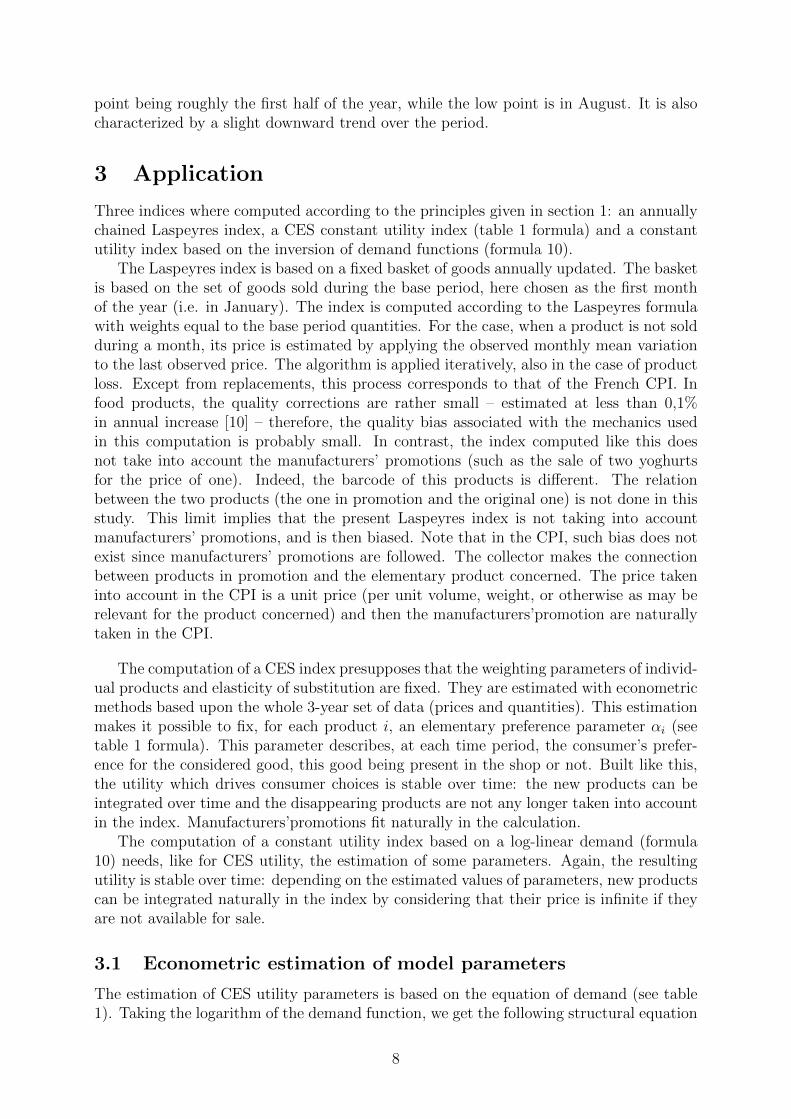
The computation of a constant utility index based on a log-linear demand (formula10) needs, like for CES utility, the estimation of some parameters. Again, the resultingutility is stable over time: depending on the estimated values of parameters, new productscan be integrated naturally in the index by considering that their price is infinite if theyare not available for sale.

3.1 Econometric estimation of model parameters

The estimation of CES utility parameters is based on the equation of demand (see table1). Taking the logarithm of the demand function, we get the following structural equation

8

(good i, time t) :

ln(xit) = ε ln(αi)︸ ︷︷ ︸ci

−ε ln(pit) + lnRt − ln

[∑k

αk

(pktαk

)1−ε]

︸ ︷︷ ︸νt

(11)

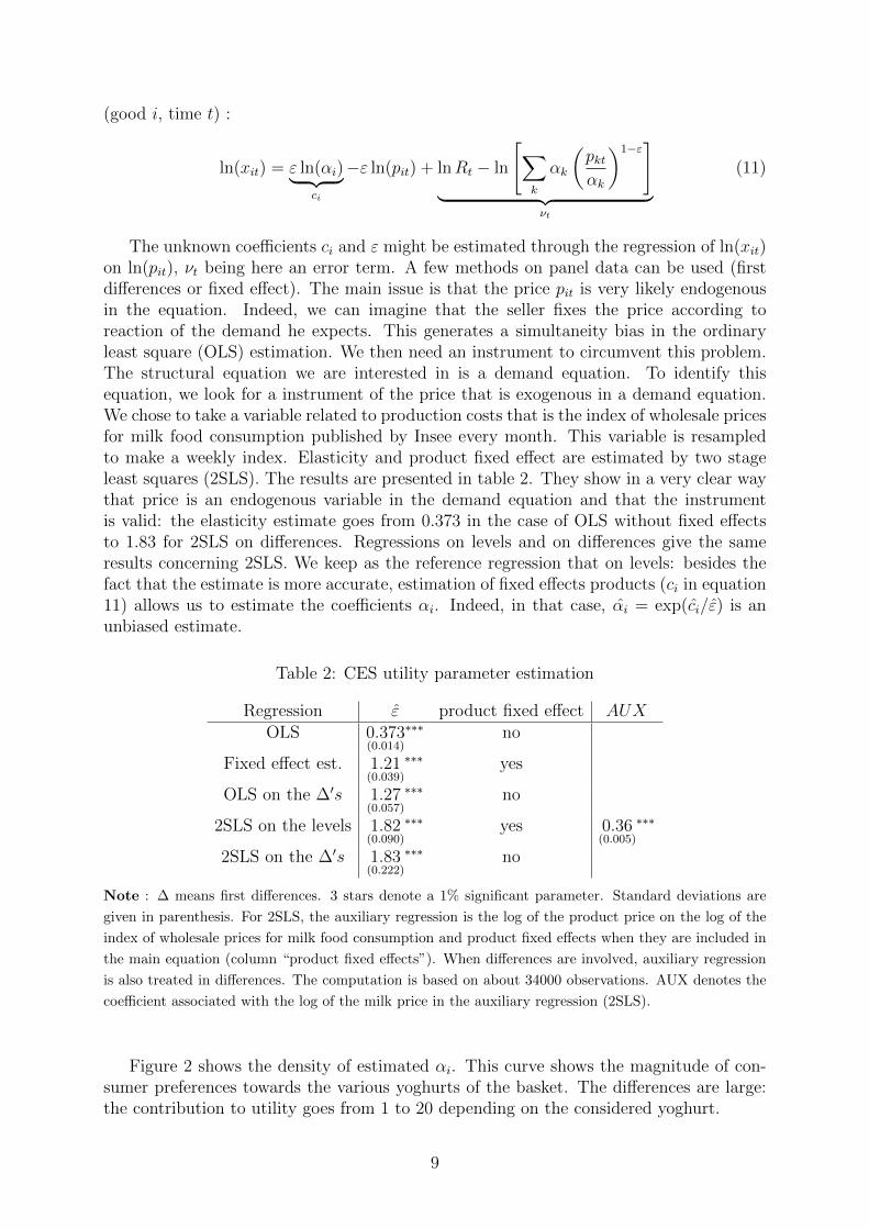
The unknown coefficients ci and ε might be estimated through the regression of ln(xit)on ln(pit), νt being here an error term. A few methods on panel data can be used (firstdifferences or fixed effect). The main issue is that the price pit is very likely endogenousin the equation. Indeed, we can imagine that the seller fixes the price according toreaction of the demand he expects. This generates a simultaneity bias in the ordinaryleast square (OLS) estimation. We then need an instrument to circumvent this problem.The structural equation we are interested in is a demand equation. To identify thisequation, we look for a instrument of the price that is exogenous in a demand equation.We chose to take a variable related to production costs that is the index of wholesale pricesfor milk food consumption published by Insee every month. This variable is resampledto make a weekly index. Elasticity and product fixed effect are estimated by two stageleast squares (2SLS). The results are presented in table 2. They show in a very clear waythat price is an endogenous variable in the demand equation and that the instrumentis valid: the elasticity estimate goes from 0.373 in the case of OLS without fixed effectsto 1.83 for 2SLS on differences. Regressions on levels and on differences give the sameresults concerning 2SLS. We keep as the reference regression that on levels: besides thefact that the estimate is more accurate, estimation of fixed effects products (ci in equation11) allows us to estimate the coefficients αi. Indeed, in that case, αi = exp(ci/ε) is anunbiased estimate.

Table 2: CES utility parameter estimation

Regression ε product fixed effect AUXOLS 0.373

(0.014)

∗∗∗ no

Fixed effect est. 1.21(0.039)

∗∗∗ yes

OLS on the ∆′s 1.27(0.057)

∗∗∗ no

2SLS on the levels 1.82(0.090)

∗∗∗ yes 0.36(0.005)

∗∗∗

2SLS on the ∆′s 1.83(0.222)

∗∗∗ no

Note : ∆ means first differences. 3 stars denote a 1% significant parameter. Standard deviations are

given in parenthesis. For 2SLS, the auxiliary regression is the log of the product price on the log of the

index of wholesale prices for milk food consumption and product fixed effects when they are included in

the main equation (column “product fixed effects”). When differences are involved, auxiliary regression

is also treated in differences. The computation is based on about 34000 observations. AUX denotes the

coefficient associated with the log of the milk price in the auxiliary regression (2SLS).

Figure 2 shows the density of estimated αi. This curve shows the magnitude of con-sumer preferences towards the various yoghurts of the basket. The differences are large:the contribution to utility goes from 1 to 20 depending on the considered yoghurt.

9

Like for CES utility parameter estimation, the estimates of the log-linear demandparameters are based on demand equation (8). Taking the logarithm, we get a structuralequation:

ln(xit) = γi + αi ln(pit) + β ln(Rt) (12)

We estimate the coefficient by regressing ln(xit) on ln(pit) and ln(Rt).

Figure 2: Density of αi coefficients of equation 11 (product weight in CES utility)

Note : coefficients αi are based on fixed effects coefficients ci in the 2SLS regression on the levels and

come from the relation: αi = exp(ci/ε). Smoothing by kernel estimation.

However, as before, the logarithm of the price pit is endogenous in the regression forthe same reasons as those mentioned in connection with the CES utility. We only haveone instrument for the whole set of product prices, therefore we are not able to identifythe whole set of αi coefficients. But if we assume that all αi are identical, then the aboveequation simplifies to:

ln(xit) = γi + α ln(pit) + β ln(Rt) (13)

This equation is identifiable if the expenditure Rt is exogenous in the equation or if wehave an instrument for it. We could imagine some cause for endogeneity: for example, ifthe consumer is price taker, then the seller is likely to fix its price in order to maximiseits profit (that is also the consumer expenditure), knowing the consumer reaction to pricechange. In that case, quantities result from the simultaneous determination of prices,quantities and expenditure.We try to test the endogeneity of the expenditure variablewith the help of an instrument of this variable in a demand equation, that is to say witha variable that is correlated with the expenditure but that do not play any role in thedemand equation.

10

For example, a wage variable would not be appropriate, because if it is actually cor-related with expenditure, it is likely that it plays a role in the demand. The variable weuse is a binary variable indicating the end of the month. Indeed, in terms of demanddeterminants, there is no indication that the end of the month is a special time to buyyoghurt. However, since the wages are usually paid in the last week of the month, thelast part of the month is probably a period xhen the budget constraint is heavier forconsumers. A binary variable indicating the end of the month (wee took the period fromthe 23th to the 30th) is then a good candidate for instrument: empirically, this variableis negatively correlated with expenditure (see column “AUX2” in table 3). However, wecan see the the instrument is not very powerful since the standard deviations of the ex-penditure coefficient in the 2SLS regression are much larger than the ones we get withOLS. Finally, a Hausman test shows that expenditure is not endogenous in the demandequation. We select the 2SLS regression on the levels with an instrument for prices only(regression “2SLS on the levels (2)” in table 3).

Table 3: Estimation of the log-linear demand parameters

Regression α β product fixed effect AUX1 AUX2

OLS on the levels −1.13(0.04)

∗∗∗ 1.09(0.02)

∗∗∗ yes

OLS on ∆′s −1.19(0.06)

∗∗∗ 1.00(0.03)

∗∗∗ no

2SLS on the levels −2.00(0.18)

∗∗∗ 0.67(0.42)

∗ yes 0.26(0.02)

∗∗∗ −0.017(0.002)

∗∗∗

2SLS on ∆′s −1.21(1.26)

2.51(1.63)

∗ no 0.24(0.03)

∗∗∗ −0.005(0.001)

∗∗∗

2SLS on the levels (2) −1.86(0.10)

∗∗∗ 1.08(0.02)

∗∗∗ yes 0.26(0.02)

∗∗∗

Note : ∆ means first differences. 3 stars denote a 1% significant parameter; 1 star denotes a 15%

significant parameter. Standard deviations are given in parenthesis. For 2SLS, the auxiliary regressions

are: 1) the log of the product price on the log of the index of wholesale prices for milk food consumption;

2) the log of expenditure on the binary variable indicating the end of the month. When differences are

involved, auxiliary regression is also treated in differences. The computation is based on about 34000

observations. AUX1 is the coefficient associated with the log of the milk price in the auxiliary regression ;

AUX2 is the coefficient of the binary variable indicating the end of the month in the auxiliary regression

of the log of expenditure. (2) : regression without expenditure instrumentation.

As for the CES index, the index based on log-linear demand makes it possible to treatincoming and outgoing products through a natural way, considering that the price of miss-ing products is infinite. Figure 3 gives de density of γi coefficients based on specification(13) for the reference regression. These coefficients are all negative and their spread goesfrom 0 to −6. This means that the weight of products in terms of contribution to theindex (see relation 10) is 1 to 1/400.

11

Figure 3: Density of Eq. 13 γi coefficients (constant multiplier of log-linear demand)

Note : The coefficients correspond to the fixed effects of the 2SLS regression with auxiliary regression

for prices, the expenditure being taken as exogenous. Smoothing by kernel estimation.

12

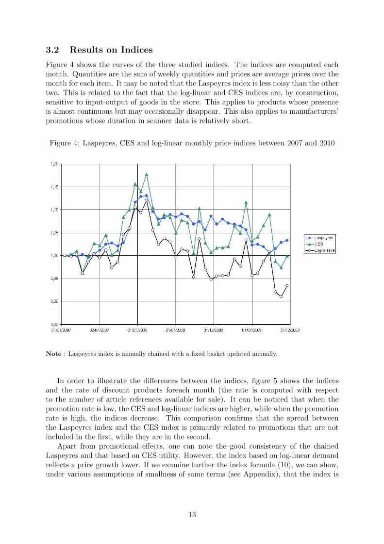
3.2 Results on Indices

Figure 4 shows the curves of the three studied indices. The indices are computed eachmonth. Quantities are the sum of weekly quantities and prices are average prices over themonth for each item. It may be noted that the Laspeyres index is less noisy than the othertwo. This is related to the fact that the log-linear and CES indices are, by construction,sensitive to input-output of goods in the store. This applies to products whose presenceis almost continuous but may occasionally disappear. This also applies to manufacturers’promotions whose duration in scanner data is relatively short.

Figure 4: Laspeyres, CES and log-linear monthly price indices between 2007 and 2010

Note : Laspeyres index is annually chained with a fixed basket updated annually.

In order to illustrate the differences between the indices, figure 5 shows the indicesand the rate of discount products foreach month (the rate is computed with respectto the number of article references available for sale). It can be noticed that when thepromotion rate is low, the CES and log-linear indices are higher, while when the promotionrate is high, the indices decrease. This comparison confirms that the spread betweenthe Laspeyres index and the CES index is primarily related to promotions that are notincluded in the first, while they are in the second.

Apart from promotional effects, one can note the good consistency of the chainedLaspeyres and that based on CES utility. However, the index based on log-linear demandreflects a price growth lower. If we examine further the index formula (10), we can show,under various assumptions of smallness of some terms (see Appendix), that the index is

13

Figure 5: Laspeyres, CES and log-linear monthly price indices and rate of discount prod-ucts

Note : Arrows indicate the months with higher promotion rate (resp. low discount rate), depending on

the case, which in turn leads to low (resp. high) prices.

14

approximately equal to:

I t′,tLogLin ' 1 +

∑i∈◦I

ωitpit′ − pitpit

+

1

1 + α

∑i∈◦I

ωit −∑i∈◦I

ωit′

+1− β1 + α

Rt′ −Rt

Rt

1−∑i∈◦I

ωit

(14)

where◦I is the set of all the products present at all observation dates, ωit is the product

i weight 2 in the expenditure at the time t, the latter being denoted Rt. The first termin this expression is a Laspeyres index, restricted solely to the goods present at time t

(basis) and t′ (in practice, we define◦I, with the help of all goods present at all dates).

Empirically, the corresponding price index, shown in Figure 6, reflects a positive changein prices over the period of observation. The first term of (14) is then positive. For theproducts always present, the trajectory of the price index is similar to that of the chainedLaspeyres index shown in Figure 4, this one being related to all goods.

The two other terms of (14) are related, on the one hand to the variation of weights inthe contemporary expenditure, of the products always present and, on the second hand,to total expenditure variations. Empirically, the weights of always present products isrelatively stable over the period 2007-2009 (see figure 7). A larger variability can be seenin 2009 due, inter alia, to a greater sensitivity of weights to promotion rates, probablyreflecting more frequent substitutions. The decrease in the weight of the products onall dates occurs mainly in the last quarter of 2009. The second term of (14) is thenempirically negative.

Finally, we observe (see figure 1) a downward trend of expenditure throughout thereporting period. Since α < −1 and β > 1, the last terme of (14) is negative.

Economically, the second term of (14) represents the effect of substitutions, while thelast term is sensitive to changes in overall spending. When utility is homothetic, thisterm vanishes. In this case, given the estimated values for α and β, a decline in spendingis associated with a utility gain ; in this context, the yoghurts are akin to an inferiorgood. The numerical computation presented in appendix shows that the magnitude ofsubstitution effect is twice larger than that related to the decreasing trend of expenditure.

4 Conclusion

Three different approaches are possible to construct a price index. The first, the classicalapproach, is based mainly on the ad hoc properties a price index should follow, theseproperties being inherited from the properties satisfied by a sequence of successive price ofa product [8]. This approach, called axiomatic approach [20], is that which prevails todayin the construction of “official” CPI. The second approach is to derive the index formulaafter the adoption of a utility function which is supposed to drive the choices made by arepresentative consumer. The parameters of the utility function are estimated from theobservation of both prices and quantities. The third approach is based on observation andparameterization of the demand functions from which we infer a constant utility index.The last two approaches are possible only with scanner data. For many years economistshave examined the differences between the indices based on the axiomatic approach, easy

2At any time t,∑

i ωit = 1.

15

Figure 6: Laspeyres Index for product always present

Note : there are about 200 references of articles always present. The products that are always present

over the 2007-2009 period represent approximatively 35% of the products (see figure 7).

Figure 7: Weight in total expenditure of the products that are always present

16

to use and easy to explain, and the constant utility index, satisfactory from an economicpoint of view, but which requires rarely available elements, on demand functions, to becomputed. If the link between the two types of index is known for a long time [6] , therecent availability of scanner data makes it possible to reconsider putting into practicethe concept of constant utility index. The first results show that the computation mightbe simplified, particularly with regard to replacement of products. Beyond this, muchremains to be done to measure in detail the implications of the econometric estimationof parameters on the computed index. Ideally, it would be good also to overcome someassumptions which are not always justified, for example on a specific utility function.Thenon-parametric approach could therefore constitute a goal in the use of scanner data.

References

[1] Arrow, K. J., Chenery, H. B., Minhas, B. S., and Solow, R. M. Capital-labor substitution and economic efficiency. The Review of Economics and Statistics43, 3 (1961), 225–250.

[2] Balk, B. On Curing the CPI’s Substitution and New Goods Bias. Discussion paper,The Ottawa Group, 1995, 1999.

[3] Boskin, M. J., Dulberger, E. R., Gordon, R. J., Griliches, Z., andW.Jorgenson, D. Consumer Prices, the Consumer Price index, and the Costof Living. Journal of Economic Perspectives 12, 1 (1998), 3–26.

[4] Clerc, E., and Coudin, E. L’IPC, miroir de l’evolution du cout de la vie enFrance ? Ce qu’apporte l’analyse des courbes d’Engel. Economie et Statistique 433–434 (2010), 77–105.

[5] Deaton, A., and Muelbauer, J. Economics and consumer behavior. CambridgeUniversity Press, 1980.

[6] Diewert, E. Aximoatic and economic approaches to elementary price indexes.Working paper 5104, NBER, 1995.

[7] Diewert, E. Index Number Issues in the Consumer Price Index. Journal of Eco-nomic Perspectives 12, 1 (1998), 47–58.

[8] Eichhorn, W., and Voeller, J. Theory of the Price Index. Springer-Verlag,1976.

[9] Feenstra, R. C., and Shapiro, M. D. High-Frequency Substitution and theMeasurement of Price Indexes. University of Chicago Press, 2003, pp. 123–146.

[10] Guedes, D. Impact des ajustement de qualite dans le calcul de l’indice des prix ala consommation. Document de travail F0404, INSEE, 2004.

[11] Hamming, R. Digital Filters, 3 ed. Dover, 1997.

[12] Hausman, J. Exact consumer’s surplus and deadweight loss. The American Eco-nomic Review 71, 4 (1981), 662–676.

17

[13] Hausman, J. Exact Consumer’s Surplus and Deadweight Loss. American EconomicReview 71, 4 (1981), 662–676.

[14] Hausman, J. Sources of Bias and Solutions to Bias ind the Consumer Price Index.Journal of Economic Perspectives 17, 1 (2003), 23–44.

[15] Hausman, J., and Leibtag, E. Consumer benefits from increased competition inshopping outlets : measuring the effect of WAL-MART. Journal of Applied Econo-metrics 22 (2007), 1157–1177.

[16] Hausman, J. A., and Newey, W. K. Nonparametric Estimation of Exact Con-sumers Surplus and Deadweight Loss. Econometrica 63, 6 (1995), 1445–1476.

[17] Hausman, J. A., Pakes, A., and Rosston, G. L. Valuing the Effect of Reg-ulation on New Services in Telecommunications. Brookings Papers on EconomicActivity, Microeconomics (1997), 1–54.

[18] Herpin, N., and Verger, D. Consommation et modes de vie en France, 3 ed. LaDecouverte, 2008.

[19] Hurwicz, L., and Uzawa, H. On the integrability of demand functions. InPreferences, Utility, and Demand (1971), J. S. Chipman, L. Hurwicz, M. K. Richter,and H. F. Sonnenschein, Eds., Harcourt, pp. 114–148.

[20] ILO, IMF, OECD, UNECE, Eurostat, and The World Bank. Consumerprice index manual : Theory and Practise. International Labour Office, 2004.

[21] Magnien, F., and Pougeard, J. Les indices a utilite constante : une referencepour mesurer l’evolution des prix. Economie et Statistique 335 (2000), 81 – 94.

[22] Mesler, D. Accounting for the effects of new and disappearing goods using scannerdata. Review of Income and Wealth 52, 4 (2006), 547–568.

[23] Moulton, B. R., and Stewart, K. J. An Overview of Experimental U.S. Con-sumer Price Indexes. Journal of Business & Economic Statistics 17, 2 (1999), 141–151.

[24] Varian, H. The Nonparametric Approach to Demand Analysis. Econometrica 50,4 (1982), 945–973.

[25] Varian, H. R. Microeconomic Analysis. The MIT Press, 1975.

[26] Varian, H. R. Trois evaluation de l’impact “social” d’un changement de prix.Cahiers du seminaire d’econometrie, 1982.

[27] Viglino, L. Le concept unificateur des indices de prix et proposition d’un nouvelindice. In Actes des journees de methodologie statistique (2000), INSEE.

18

Appendix: computational developments

Solving of the partial differential equation system (6) for demandfunctions (8)

We must solve in µ the following set of differential equations :

1 6 i 6 n ,∂µ

∂pi= pαii µ

βeγi

For i, we have in particular ∂µ∂pi

= pαii µβeγi which can be solved, partially, by integrating

on pi :µ1−β

1− β=

p1+αii

1 + αieγi + Ci(p(i); q, R)

where Ci is a function depending on p(i) (vector of prices p without the ith component),on q and on R. We can therefore seek a solution of the form

µ(p; q, R) =

{(1− β)

[n∑i=1

p1+αii

1 + αieγi + C(q, R)

]} 11−β

where C is a function depending on q and R. It can be found using the limit condition(see relation 7) µ(q; q, R) = R, so:

C(q, R) =R1−β

1− β−

n∑i=1

q1+αii

1 + αieγi

Finally,

µ(p; q, R) =

{(1− β)

[R1−β

1− β+

n∑i=1

eγi .p1+αii − q1+αi

i

1 + αi

]} 11−β

Approximation of the log-linear index (14)

The proof is based on the assumption that pit − pit′ , Rt − R′t, ωit − ωit′ and that the

complement to 1 of the index I t′,tLogLin are infinitesimals of first order. We also suppose

that all the αi are equal to a unique α (framework of econometrics). Starting from (10),to the first order, we have :

I t′,tLogLin ' 1 +Rβ−1

t

n∑i=1

eγip1+αit′ − p

1+αit

1 + α

If we note I t the set of products present at time t, it is possible to define the intersection◦I of these sets for all the dates. Thus defined,

◦I corresponds to the set of the products

that are always present. For all t, one note I t the complement to◦I in I t. The previous

relation can then be written:

I t′,tLogLin ' 1 +Rβ−1

t

∑i∈◦I

eγip1+αit′ − p

1+αit

1 + α+Rβ−1

t

∑i∈It′

eγip1+αit′

1 + α−Rβ−1

t

∑i∈It

eγip1+αit

1 + α

19

PThen, at any time t, the budget constraint implies∑pitxit = Rt. Taking into account

the expression of demand function (relation 8), it follows that ωit = Rβ−1t p1+α

it eγi is thegood i weight in the expenditure Rt at time t.

For i ∈◦I, by a Taylor expansion to first order in pit′ − pit, we have :

p1+αit − p1+α

it ' (1 + α)pαit(pit′ − pit)

It follows that:

Rβ−1t

∑i∈◦I

eγip1+αit′ − p

1+αit

1 + α'∑i∈◦I

ωitpit′ − pitpit

Then, the other terms are simplified by using the budget constraint and the fact that thesum of weights is 1 for a given time t. Thus:

Rβ−1t

∑i∈It

eγip1+αit

1 + α=

1

1 + α

1−∑i∈◦I

ωit

Similarly,

Rβ−1t

∑i∈It

eγip1+αit′

1 + α=

1

1 + α

(Rt

Rt′

)β−11−

∑i∈◦I

ωit′

The last expression can be simplified on the basis of the assumptions that the differencesRt′ −Rt and ωit − ωit′ are small. Indeed,

1

1 + α

(Rt

Rt′

)β−11−

∑i∈◦I

ωit′

=1

1 + α

(1 +

Rt′ −Rt

Rt

)1−β1−

∑i∈◦I

ωit +∑i∈◦I

(ωit − ωit′)

By developing to the first order and summing the result with the other two terms alreadyexplained, we have:

I t′,tLogLin ' 1 +

∑i∈◦I

ωitpit′ − pitpit

+

1

1 + α

∑i∈◦I

ωit −∑i∈◦I

ωit′

+1− β1 + α

Rt′ −Rt

Rt

1−∑i∈◦I

ωit

numerical computation : we adopt the following numerical values

•∑

i∈◦Iωit = 0.45

• 1∑i∈◦Iωit

∑i∈◦Iωit

pit′−pitpit

= 0.05

• α = −1.86

• β = 1.08

•∑

i∈◦I(ωit−ωit′) = 0.46− 0.44 = 0.02 (mean difference of the first and last semesters

of observation)

20

With these numbers,

I2009S2,2007S1LogLin ' 1 + 0.45× 0.05︸ ︷︷ ︸

0.02

− 1

0.86× 0.02︸ ︷︷ ︸

0.02

− 0.08

0.86× 0.2× (1− 0.45)︸ ︷︷ ︸

0.01

' 1− 0.01

As expected, the index I t′,2007LogLin is negative for the last semester of 2009. This compu-

tation allows us to derive the contributions: the Laspeyres index of the goods that arealways present contributes positively to 2 points; the decrease of the total expenditurecontributes negatively to 1 point; and substitutions contribute negatively to 2 points.Finally, according to this index, prices have decreased over the period;

21