Scaling Agricultural Policy Interventions:

Theory and Evidence from Uganda∗

Lauren Falcao Bergquist†, Benjamin Faber‡, Thibault Fally§,

Matthias Hoelzlein¶, Edward Miguel‖, Andres Rodriguez-Clare∗∗

November 2019

–Preliminary and Incomplete–

Interventions aimed at raising agricultural productivity in developing countries have been a cen-

terpiece in the global fight against poverty. These policies are increasingly informed by evidence

from field experiments and natural experiments, with the well-known limitation that findings

based on local variation generally do not speak to the general equilibrium (GE) effects if the

intervention were to be scaled up to the national level. In this paper, we develop a new frame-

work to quantify these forces based on a combination of theory and rich but widely available

microdata. We build a quantitative GE model of farm production and trade, and propose a new

solution method in this environment for studying high-dimensional counterfactuals at the level

of individual households in the macroeconomy. We then bring to bear microdata from Uganda

to calibrate the model to all households populating the country. We use these building blocks to

explore the average and distributional implications of local shocks compared to policies at scale,

and quantify the underlying mechanisms.

∗This research was supported by funding from the International Growth Centre (IGC). We thank Rodrigo Adao andPablo Fajgelbaum for helpful comments. All errors are our own.†Department of Economics, University of Michigan and NBER‡Department of Economics, UC Berkeley and NBER§Department of Agricultural and Resource Economics, UC Berkeley and NBER¶Department of Economics, UC Berkeley‖Department of Economics, UC Berkeley and NBER∗∗Department of Economics, UC Berkeley and NBER

1

1 Introduction

Roughly two thirds of the world’s population living below the poverty line work in agriculture.

In this context, interventions aimed at improving agricultural productivity, such as agricultural

extension campaigns providing access, information, training and/or subsidies for modern pro-

duction techniques, have played a prominent role in the global fight against poverty.1 In order

to inform these policies using rigorous evidence, much of the recent literature in this space has

used variation in household outcomes from randomized control trials (RCTs) or natural experi-

ments.

While rightly credited for revolutionizing the field of development economics, experiments

and quasi-experiments frequently face the well-known limitation that local interventions or

shocks often do not speak to the broader general equilibrium (GE) effects if the policy were to

be scaled up to cover all farmers at the regional or national levels. For example, both the average

and distributional effects of a fertilizer subsidy on household real incomes could substantially

differ between a local intervention that leaves market prices unchanged and a policy at scale

that affects output and factor prices across markets. The magnitude and distributional impli-

cations of these GE forces depend on a complex interplay of the policy’s direct effect on yields

across different crops, the pre-existing geography of household consumption and production

choices across market places in the country, the size and nature of trade costs between farmers

and local markets and across markets, the use of different factors of production across crops

and sectors, expenditure shares on crops and sectors across the income distribution, as well as

the responsiveness of production and consumption choices to the policy’s direct effect on yields

and prices.

While much has been written about the challenges of using local variation for informing

policy-making at scale (e.g. Heckman & Smith (1995), Moffitt (2009), Ravallion (2009, 2018),

Rodrik (2008), Deaton (2010)), these forces have not been studied and quantified using a com-

bination of theory and administrative microdata covering all households and market places for

the entire country.2 In this paper, we take a step in this direction through the lens of a rich but

tractable quantitative GE model of farmer-level production and trade. To capture a number of

salient features that we document in the agricultural empirical context, the model departs in

several dimensions from the workhorse ”gravity” structure of models in international trade and

economic geography. In this environment, we propose a new solution approach that allows us

to quantify GE counterfactuals without relying on structural gravity and without imposing stark

new data requirements to be able to do so. We then bring to bear administrative microdata

on pre-existing household locations, production, consumption and the transportation network

within and across local markets to calibrate the model to the roughly 6 million households pop-

ulating Uganda, and proceed to explore economy-wide GE counterfactuals at this granular level.

We use these building blocks to answer four central questions: i) To what extent do the aver-

1See e.g. Caldwell et al. (2019) for a review of recent impact evaluations in this space.2See discussion of related literature at the end of this section.

2

age and distributional effects of an agricultural policy on household welfare differ between a lo-

cal intervention and implementation at scale?; ii) How do these differences behave as a function

of increasing rates of saturation going from a small number of farmers to 100 percent coverage?;

iii) What is the role of modeling realistic trading frictions between agents in the economy, and

the nature of these frictions, for the impact of scaling up?; and iv) What is the role of modeling

individual households vs aggregating to regions or markets when quantifying the impact of scal-

ing up? To fix ideas throughout the analysis, we focus on the impact of a subsidy for modern

inputs (chemical fertilizers and hybrid seed varieties in our setting), but the framework is set up

to study other types of interventions that are targeted at increasing agricultural productivity or

farmers’ market access more generally.

Our analysis proceeds in five steps. In the first step, we use the Ugandan microdata we have

assembled described in Section 2 to document a number of stylized facts on farm production,

consumption and trade. These stylized facts inform the structure of the model we develop in the

second step. In terms of basic context, we document that farmers trade what they produce and

consume in local markets, rather than purely living in subsistence, and that farmers adjust the

share of land allocated across different crops across space and time. Using trader survey micro-

data, we find that local markets do not trade with one another on the vast majority of possible

bilateral connections, suggesting that agricultural crops are mostly not differentiated across pro-

ducers in this setting (Sotelo (2017)). We further document evidence for downward-sloping En-

gel curves in the share of agricultural consumption across rich and poor households facing the

same market prices, suggesting non-homothetic preferences and a potential for distributional

implications of GE effects on output prices. Next, we document that trade costs from farmers to

local markets and between local markets are best captured by additive unit trade costs (charged

per unit of weight) rather than ad valorem (iceberg), implying incomplete and decreasing price

pass-through as a function of distance between markets. Finally, we show that the adoption of

modern inputs, such as chemical fertilizer or hybrid seeds, changes the relative cost shares of

traditional inputs (land and labor), suggesting that adoption of modern production techniques

would not be well-captured by Hicks-neutral productivity shifts.

After laying out the model in step 2, step 3 proposes a new approach to quantifying GE coun-

terfactuals in this rich environment. To explain our approach, it is useful to compare it to what

is now standard practice using ”exact-hat algebra” in the international trade literature (see for

instance Adao et al. (2017)). This involves using the full matrix of bilateral trade flows and knowl-

edge of the key elasticities or aggregate demand functions to solve for the (hat) changes of the

endogenous variables given (hat) changes in the exogenous parameters. However, we do not

observe the universe of crop-level bilateral trade flows at the individual farmer-to-farmer level,

and even if one did have such data, it would be mostly made up of zeros, so the standard pro-

cedure would not be applicable. Instead, we show that solving for counterfactual changes in

our environment requires knowledge of the full vector of pre-existing prices faced by agents

across all markets. To address this challenge, we show that we can use estimates of trade costs

3

in combination with data on household-level expenditure shares and production quantities to

set up a ”price discovery problem”. This entails solving for equilibrium farm-gate prices and

trade flows that rationalize the observed consumption and production decisions given a graph

of trade costs connecting households and markets. In turn, with knowledge of farm-gate prices

and trade costs, we can express farmer-level excess demand functions in terms of counterfactual

prices and hat changes in farmer productivities (along with expenditure shares and production

in the original equilibrium). We then use these excess demand functions and the no-arbitrage

conditions to form a system of equations that we can use to solve for the counterfactual equilib-

rium.

This approach has several advantages. First, we are able to solve the model without relying

on structural gravity and without imposing stark new data requirements (such as observing the

full set of pre-existing market prices). Second, our solution method ensures that the economy is

in equilibrium before solving for counterfactuals: the household prices we obtain from the price

discovery are by construction consistent with the calibrated trade costs and the consumption

and production decisions we observe in the data.3 Finally, from a computational perspective

our solution method is capable of handling high-dimensional GE counterfactuals at the level of

individual households in the macroeconomy.

In step 4, we use the Ugandan microdata to calibrate the model to the roughly 6 million

households who populate the country. To calibrate cross-market trade costs, we make use of

estimates from Bergquist & McIntosh (2019), using newly collected market and trader survey

microdata to provide information on bilateral market trade flows and local market prices at ori-

gin and destination across crops. To calibrate within-market trade costs between farmers and

their local markets, we use observed gaps in the Ugandan National Panel Survey (UNPS) be-

tween farm-gate prices and local markets in combination with knowledge of farmer-level trade

flows to and from the markets. To estimate the key supply elasticity of the model, we use the

UNPS microdata and exploit plausibly exogenous changes in world market prices across differ-

ent crops that propagate differently to local markets as a function of distance from the nearest

border crossing.

In the final step, we use the calibrated model to conduct the counterfactual analysis and

present a number of additional robustness and model validation tests using natural experiments

over our sample period (road additions and weather shocks). To investigate the difference in

changes in economic outcomes across local interventions and scaling up, we randomly select

a representative sample of ten thousand rural households in Uganda (roughly 0.2 percent of

Ugandan households). We then solve for counterfactual GE changes in household-level eco-

nomic outcomes due to an intervention that only targets the subsidy for modern inputs at these

ten thousand households, and compare the effects on those same households to an intervention

that scales the subsidy policy to all rural households in the country. In particular, we investigate

3For example, Sotelo (2017) uses province-level crop unit values from agricultural surveys to calibrate and solvethe model, but these price data are not model-consistent with the calibrated trade costs.

4

differences in both the average and distributional welfare effects across households, and docu-

ment the underlying channels.

In our preliminary set of results (work in progress at the time of this writing), we find that the

average effect of a subsidy for modern inputs on rural household welfare can differ substantially

when comparing effects in the local intervention compared to effects on the same households

when scaling up to the national level. In addition, the policy’s distributional implications differ

significantly: while the local intervention is strongly regressive (benefiting initially richer ru-

ral households the most), the welfare gains are significantly more evenly distributed under the

intervention at scale. Underlying these findings, we document GE price effects on crops and

factors of production that propagate along the trading network and affect nominal incomes as

well as household price indices differently compared to the local intervention.

Recognizing that GE effects at scale can play an important role, recent empirical studies in

development economics have used two-stage cluster randomization designs (e.g. Baird et al.

(2011), Burke et al. (2019)), Egger et al. (2019)) to measure treatment effects at different levels of

saturation across clusters of markets. Due to constraints on statistical power, such designs typ-

ically limit the comparison to just two discrete levels of saturation (often chosen ad hoc). If the

aim is to extrapolate from these two points of saturation to make inference on what treatment ef-

fects would look like at 100% saturation, however, one must make the assumption that GE forces

are both monotonic and linear with respect to changes in saturation rates.4 To investigate this

question, we quantify GE effects on an identical sample of Ugandan households across various

levels of national saturation going from 0-100 percent. We find that the GE forces appear to be

both non-linear and non-monotonic as a function of the national saturation rate. This finding

suggests caution regarding unobserved non-linearities when extrapolating from the results of

randomized saturation designs to policy implications at full scale.

In the third question, we study the importance of allowing for realistic trade costs between

agents when aggregating the average and distributional implications of shocks in the macroe-

conomy. As we discuss below, the recent macroeconomics literature on aggregation mostly ab-

stracts from such frictions. To this end, we estimate two additional sets of counterfactuals (both

for the local intervention and the scaled intervention). We first re-estimate our baseline counter-

factuals after setting the trading frictions between households and local markets and across local

markets to zero. Second, we re-estimate the counterfactuals after specifying and calibrating the

model featuring ad valorem (iceberg) trading frictions, instead of our baseline counterfactuals

with additive unit costs. We find that the welfare gains from scaling up the policy are affected in

both the average and distributional effects subject to these alternative assumptions.

In the fourth question, we explore the implications of modeling households at a granular

level compared to aggregating them into different clusters of regional representative agents across

Uganda. In our preliminary results, we find that preserving trading frictions at a granular level

4Another necessary assumption for extrapolating results from randomized saturation designs to at-scale policiesis that there are no GE spillover effects across the clusters. We plan to present additional results on this question infuture versions of this draft.

5

matters for the counterfactual results.

Related Literature In addition to the references discussed above, this paper relates and con-

tributes to a number of different literatures. It relates to a large and growing number of studies

using experiments or quasi-experiments to evaluate the impact of agricultural policy interven-

tions in (e.g. Caldwell et al. (2019), Carter et al. (2014), Duflo et al. (2011), Emerick et al. (2016),

Magruder (2018)). Relative to the existing literature in this space, our objective is to study and

quantify how the impacts found in relatively small-scale interventions are subject to change if

the same intervention were to be scaled up at different levels of saturation, and to disentangle

the underlying mechanisms.5 Our hope is to provide a useful methodological toolkit that can be

used to complement the results from observed local interventions to evaluate interventions at

scale.

From a methodological point of view, our framework contributes to a growing literature in

macroeconomics that has sought to quantify the aggregation of observed local shocks if they

were to occur to all agents in the economy (e.g. Buera et al. (2017), Baqaee & Farhi (2018), Sraer

& Thesmar (2018), Fujimoto et al. (2019)). A common feature of this literature is its treatment

of the macroeconomy as one single integrated market in which all agents interact without trad-

ing frictions and face identical prices. In our framework, each household faces trading frictions

and imperfect pass-through for buying and selling output to local markets, for both goods and

factors of production, and in turn trade flows across local markets are subject to trade costs and

imperfect pass-through along the transportation network. We calibrate these trading frictions

using survey data on household farm-gate prices, local market prices and information on bilat-

eral trade flows across local markets. By studying counterfactuals before and after setting trade

costs close to zero, this allows us to investigate the importance of modeling realistic trading

frictions between agents when solving for both the average and distributional implications of a

shock in the aggregate.

Our methodology also relates to an earlier literature on computable general equilibrium

(CGE) models in development economics (see e.g. de Janvry & Sadoulet (1995) for a review).6

Our framework and analysis depart from this literature in at least three important respects. First,

due to computational constraints as well as much less availability of rich survey microdata at

the time, these models are usually based on one (or a small number of) representative agents

that make up the macroeconomy. In contrast, our framework embraces the full degree of het-

erogeneity across individual households that we observe in the initial equilibrium. Second, as

in the macroeconomics literature on aggregation discussed above, these models largely abstract

from trading frictions across households and markets, and model the economy as one integrated

market instead of local market places that are connected along a transportation graph. Third,

5See Svensson & Yanagizawa-Drott (2012) for a cautionary tale on how estimated impacts in partial and generalequilibrium can diverge for agricultural interventions in Uganda.

6This literature has also been referred to as ”multi-market” analysis, as the impact of shocks is traced across mul-tiple output and factor markets in the economy.

6

the CGE literature relied on what sometimes has been referred to as a ”black box” of numer-

ous parameters whose values determine the responsiveness to different shocks across different

sectors, output markets and factor markets. Given a large number of such parameter values,

it becomes hard to judge ex-post which of these parameter combinations affect the simulation

results and to what extent. In contrast, our model follows recent work on quantitative GE mod-

els in international trade and economic geography (e.g. Eaton & Kortum (2002)), which has the

benefit of greater tractability and transparency. Instead of dozens or hundreds of parameters

governing counterfactual results, our framework highlights a small set of key elasticities in both

production and demand, whose impact on the main findings can be readily assessed across al-

ternative parameter ranges.

Finally, our theoretical framework builds on recent work using quantitative models in inter-

national trade and economic geography (e.g. Allen & Arkolakis (2014), Redding (2016)). Given

the empirical context, we depart from the workhorse gravity structure most commonly used in

this literature. As discussed above, we therein build on recent work by e.g. Costinot & Donaldson

(2016), Fajgelbaum & Khandelwal (2016), Adao et al. (2017), Sotelo (2017) and Adao et al. (2018).

Given our focus on agriculture, the paper is in particular related to Sotelo (2017) and Costinot

& Donaldson (2016). Relative to Sotelo (2017) the main differences are that we set out to quan-

tify counterfactuals at the level of individual households rather than representative agents at the

level of provinces, and that we propose a new solution method allowing us to quantify counter-

factual changes in absence of structural gravity without imposing stark new data requirements

(such as observing pre-existing prices for all agents).7 Relative to Costinot & Donaldson (2016)

the main differences are, again, households versus regions, that we model trade flows between

all markets rather than to one national hub and that we aim at a welfare analysis (requiring a de-

mand side) rather than focusing on the production side. Finally, in terms of calibration and so-

lution method, the key source of information used by Costinot & Donaldson (2016) to construct

production possibility frontiers across crops –the FAO GAEZ database– would not be suitable for

an analysis at the household level.8

The remainder of the paper is structured as follows. Section 2 presents the data and stylized

facts. Section 3 develops the model and the solution method. Section 4 presents the calibra-

tion. Section 5 presents the counterfactual analysis, robustness and model validation. Section 6

concludes.

7Our framework also differs by allowing for non-homothetic preferences, additive trade costs and different tech-nology regimes in production.

8In the case of Uganda, FAO GAEZ covers roughly 2100 5-minute arc grid cells (> 100km2 on average). In contrast,the survey data suggest rich variation in crop suitability across small plots of land (including within farmers), a featurethat our model and calibration aim to embrace.

7

2 Data and Stylized Facts

In this section we briefly describe the database we have assembled. We then use these data to

document the empirical context and a number of stylized facts.

2.1 Data

Our analysis makes use of four main datasets.

Uganda National Panel Survey (UNPS)

The UNPS is a multi-topic household panel collected by the Ugandan Bureau of Statistics as

part of the World Bank’s Living Standards Measurement Survey. The survey began as part of the

2005/2006 Ugandan National Household Survey (UNHS). Then starting in 2009/2010, the UNPS

set out to track a nationally representative sample of 3,123 households located in 322 enumer-

ation areas that had been surveyed by the UNHS in 2005/2006. The UNPS is now conducted

annually. Each year, the UNPS interviews households twice, in visits six months apart, in order

to accurately collect data on both of the two growing seasons in the country. In particular, the

main dataset that we assembled contains 77 crops across roughly 100 districts and 500 parishes

for the periods 2005, 2009, 2010, 2011 and 2013. It includes detailed information on agriculture,

such as cropping patterns, crop prices, amount of land, amount of land allocated to each crop,

labor and non-labor inputs used in each plot and technology used at the household-parcel-

plot-season-year. Data on consumption of the household contains disaggregated information

on expenditures, consumption quantities and unit values.

Uganda Population and Housing Census 2002

The Ugandan Census has been conducted roughly every ten years since 1948. Collected by the

Ugandan Bureau of Statistics, it is the major source of demographic and socio-economic statis-

tics in Uganda. Over the span of seven days, trained enumerators visited every household in

Uganda and collected information on all individuals in the household. At the household level,

the Census collects the location (down to the village level), the number of household members,

the number of dependents, and ownership of basic assets. Then for each household member,

the Census collects information on the individual’s sex, age, years of schooling obtained, literacy

status, and source of livelihood, among other indicators. We have access to the microdata for the

100 percent sample of the Census.

Survey Data on Cross-Market Trade Flows and Trade Costs

The survey data collected by Bergquist & McIntosh (2019)) can be used to shed light on cross-

market trade flows and calibrate between-market transportation costs. They collect trade flow

8

data in a survey of maize and beans traders located in 260 markets across Uganda (while not

nationally representative, these markets are spread throughout the country). Traders are asked

to list the markets in which they purchased and the markets in which they sold each crop over

the previous 12 months. This information can be used to limit the calibration of cross-market

trade costs to market pairs between which there were positive trade flows over a given period.

They complement this data with a panel survey, collected in each of the 260 markets every two

weeks for three years (2015-2018) in which prices are collected for maize, beans, and other crops.

A greater description of the data collection can be found in Bergquist & McIntosh (2019).

GIS Database and World Prices

We use several geo-referenced datasets. We use data on administrative boundaries and detailed

information on the transportation network (covering both paved and non-paved feeder roads)

from Uganda’s Office of National Statistics. We complement this database with geo-referenced

information on crop suitability from the Food and Agricultural Organization (FAO) Global Ago-

Ecological Zones (GAEZ) database. This dataset uses an agronomic model of crop production to

convert data on terrain and soil conditions, rainfall, temperature and other agro-climatic condi-

tions to calculate the potential production and yields of a variety of crops. We use this informa-

tion as part of the projection from the UNPS sample to the Ugandan population at large. Finally,

we use information on world crop prices (faced by other African nations over time) from the FAO

statistics database.

2.2 Context and Stylized Facts

Major Crops, Regional Specialization and Price Gaps, Subsistence, Trading and Land

Allocations

Appendix Figures A.1, A.2 and Tables A.1-A.5 present a number of basic stylized facts about the

empirical context. Unless otherwise stated, these are drawn from the UNPS panel data of farm-

ers. First, Table A.1 documents that the 9 most commonly grown crops (matooke (banana),

beans, cassava, coffee, groundnuts, maize, millet, sorghum and sweet potatoes) account for 99

percent of the land allocation for the median farmer in Uganda (and for 86 percent of the aggre-

gate land allocation).

Second, Figure A.1 and Table A.2 document a significant degree of regional specialization in

Ugandan agricultural production across regions. Table A.2 provides information that these re-

gional differences translate into meaningful variation in regional market prices across crops: the

across-district variation in average crop prices accounts for 20-60 percent of the total variation

in observed farm-gate prices.

Third, Table A.3 documents that the majority of all farmers are either net sellers or net buy-

ers, rather than in subsistence, and this holds across each of the 9 major crops. The table also

presents evidence that there are significant movements in and out of subsistence, conditional on

9

having observed subsistence at the farmer level in a given season. Fourth, Table A.4 documents

that farmers buy and sell their crops mostly in local markets, which in turn are connected to

other markets through wholesale traders. Finally, Table A.5 documents that farmers frequently

reallocate their land allocations across crops over time.

Product Differentiation Across Farmers

Appendix Table A.6 looks at evidence on product differentiation across farmers. The canonical

approach in models of international trade sets focus on trade in manufacturing goods across

countries, where CES demand coupled with product differentiation across manufacturing vari-

eties imply that all bilateral trading pairs have non-zero trade flows. In an agricultural setting,

however, and focusing on households instead of entire economies, this assumption would likely

be stark. Consistent with this, the survey data collected by Bergquist & McIntosh (2019) suggest

that less than 5 percent of possible bilateral trading connections report trade flows in either of

the crops covered by their dataset (maize and beans). This finding reported in Table A.6 pro-

vides corroborating evidence that agricultural crops in the Ugandan empirical setting are un-

likely well-captured by the assumption of product differentiation across farmers who produce

the crops.

Household Preferences

Appendix Figure A.2 reports a non-parametric estimate of the household Engel curve for food

consumption. We estimate flexible functional forms of the following specification:

FoodShareit = f (Incomeit) + θmt + εit

where θmt is a parish-by-period fixed effect and f(Incomeit) is a potentially non-linear function

of household i’s total income in period t. The inclusion of market (parish)-by-period fixed effects

implies that we are comparing how the expenditure shares of rich and poor households differ

while facing the same set of prices and shopping options. As reported in the figure, the average

food consumption share ranges from 60 percent among the poorest households to about 20

percent among the richest households within a given market-by-period cell.

Nature of Trade Costs

The magnitude and nature of trade costs between farmers and local markets and across local

markets play an important role for the propagation of output and factor price changes between

markets along the transportation network. The canonical assumption in models of international

trade is that trade costs are charged ad valorem (as a percentage of the transaction price). Ad val-

orem trade costs have the convenient feature that they enter multiplicatively on a given bilateral

route, so that the pass-through of cost shocks at the origin to prices at the destination is com-

10

plete (the same percentage change in both locations). In contrast, unit trade costs –charged per

unit of the good, e.g. per sack or kg of maize– enter additively and have the implication that

price pass-through is a decreasing function of the unit trade costs paid on bilateral routes. Mar-

ket places farther away from the origin of the cost shock experience a lower percentage change

in destination prices, as the unit cost makes up a larger fraction of the destination’s market price.

To explore the nature of trade costs across Ugandan markets, we replicate results reported in

Bergquist & McIntosh (2019). Specifically, we estimate:

todkt = (pdkt − pokt) = α+ βpokt + θod + φt + εodkt

where todkt are per-unit trade costs between origin o and destination d for crop k (maize or beans)

observed in month t, pokt are origin unit prices, θod are origin-by-destination fixed effects, and φtare month fixed effects. Alternatively, origin-by-destination-by-month fixed effects (θodt) can be

included.

Following Bergquist & McIntosh (2019), we estimate these specifications conditioning on

market pairs for which we observe positive trade flows in a given month. If trade costs include

an ad valorem component, we would expect the coefficient β to be positive and statistically

significant. On the other hand, if trade costs are charged per unit of the shipment (e.g. per sack),

we would expect the point estimate of β to be close to zero.

One concern when estimating these specifications is that the origin crop price pokt appears

both on the left and the right-hand sides of the regression, giving rise to potential correlated

measurement errors. This would lead to a mechanical negative bias in the estimate of β. To

address this concern, we also report IV estimation results in which we instrument for the ori-

gin price in a given month with the price of the same crop in the same market observed in the

previous month.

As reported in Table A.7, we find that β is slightly negative and statistically significant in the

OLS regressions, but very close to zero and statistically insignificant after addressing the concern

of correlated measurement errors in the IV specification. Taken together with existing evidence

from field work (e.g. Bergquist (2017)), these results suggest that trade costs in this empirical

setting are best-captured by per-unit additive transportation costs.

Modern Technology Adoption

Many policy interventions that are run through agricultural extension programs are aimed at

providing access, information, training and/or subsidies for modern technology adoption among

farmers. One important question in this context is whether adopting modern production tech-

niques could be captured by a Hicks-neutral productivity shock to the farmers’ production func-

tions for a given crop. Alternatively, adopting modern techniques could involve more compli-

cated changes in the production function, affecting the relative cost shares of factors of produc-

tion, such as land and labor.

11

To provide some descriptive evidence on this question, we run specifications of the following

form:

LaborShareikt = α+ βModernUseikt + θm + φk + γt + εikt

where LaborShareikt is farmer i’s the cost share of labor relative to land (including both

rents paid and imputed rents) for crop k in season t (there are two main seasons per year),

ModernUseikt is an indicator whether the farmer uses modern inputs for crop k in season t (de-

fined as chemical fertilizer or hybrid seeds), and θmkt, φk and γt are district, crop and season

fixed effects. Alternatively, we also include individual farmer fixed effects (θi).

As reported in appendix Table A.8, we find that the share of labor costs relative to land costs

increases significantly as a function of whether or not the farmer uses modern production tech-

niques. This holds both before and after the inclusion of farmer fixed effects (using variation

only within-farmer across crops or over time). These results suggest that modern technology

adoption is unlikely to be well-captured by a simple Hicks-neutral productivity shift in the pro-

duction function.

3 Model and Solution Method

In this section we develop a rich but tractable GE model of farm production and trading that

is able to capture the stylized facts we document in Section 2 above. We present a model that

features heterogeneous producers and consumers who interact across a complex geography.

The economy is populated by farmers that are endowed with land of heterogeneous suitabil-

ity for different homogeneous crops. These producers choose an optimal land allocation across

crops taking output and input prices as given. Price differences are driven by trade costs across

farmers and their local markets as well as trade costs across local markets that weaken special-

ization and induce some farmers to stay in subsistence farming for certain crops. Trade costs

also reduce the amount of modern intermediate inputs, like fertilizer, used in production. Trade

costs are driven by the farmer’s location relative to the local market and the position of the local

market relative to the rest of the economy.

Farmers are assigned to a local market and can trade goods and labor on that market. These

local markets are connected with all other markets and the rest of the world by a graph based

on existing infrastructure. Given increasing policy attention to promoting modern technology

adoption, like the usage of chemical fertilizer or hybrid seed varieties, the model allows farmers

to change their production technology in response to an intervention. We further augment the

model by introducing a homogeneous and tradable manufacturing good produced by urban

households. The economy is small in the sense that it does not affect international prices of

crops, the manufacturing good, or the agricultural intermediate good in the rest of the world.

In contrast to the standard approach in the literature, and consistent with the stylized fact

presented in the previous section, we assume that trade costs have both an additive and an

iceberg component, and that preferences are non-homothetic. Additive trade costs are in terms

12

of some good (e.g., gasoline) that is imported from the rest of the world, and hence its price

is not affected by our small economy. This will simplify our analysis since we do not need trace

potential effects of the scaling up of the intervention on local trade costs across the geography of

Uganda. As in most of the development literature, we allow for non-homotheticity in preferences

to capture the large disparity in the share of income spent on food, and allowing for potential

distributional implications through the price index.

Environment

There are two kinds of agents, farmers (indexed by i) and urban households (indexed by h), and

two kinds of markets, villages (indexed by v) and urban centers (indexed by u). There will also be

an agent that we call Foreign (denoted by F ) and stands for the rest of the world. In general, each

of these nodes (farmers or markets) in the economy is indexed by o (origin) or d (destination)

when dealing with the trade network, and with j (households i or h or Foreign F ) or m (market)

when dealing with agent behavior or market clearing conditions, respectively.

These nodes trade in outputs (k ∈ K) and inputs (n ∈ N ). The are two kinds of outputs,

agricultural goods (k ∈ KA) and a manufacturing good (k = M ), and two kinds of inputs, inter-

mediate goods (n ∈ N I) and labor (n = L). We use g as a generic index that encompasses both

outputs and inputs, hence g ∈ G ≡ K ∪N .Farmers own land and labor in quantities Zi and Li, and they produce agricultural goods

using their own land (i.e., land is not tradable) as well as labor and intermediate goods. Urban

households own labor in quantity Lh and produce the manufacturing good using labor. Inter-

mediate goods are imported from Foreign.

Let Og (d) denote the set of origin nodes from where node d can obtain good g and Dg (o)

denote the set of destination nodes which can obtain good g from node o. In other words, trade

in good g from o to d only happens if o ∈ Og (d) or, equivalently, d ∈ Dg (o). We assume that

a farmer i can trade only with the village v in which she is located, that is, Og (i) = Dg(i) =

v for all g. Similarly, an urban household h can trade only with the urban center u in which

it is located, that is, Og (h) = Dg(h) = u for all g. Further, while each village can consist

of multiple farmers, each urban center consists of one representative household. Labor is not

tradable across markets, i.e., m′ /∈ OL (m) for all markets m 6= m′.

Let pj,g denote the price at which agent j buys or sells good g, and let pm,g is the price at

which good g is bought or sold at market m. Trade in good g from o to d ∈ Dg (o) is subject to

iceberg and additive trade costs. Iceberg trade costs are τod,g and additive trade costs are tod,g in

units units of a “transportation good.” We use index T for this transportation good and assume

that it is produced by Foreign at price p∗F,T , and further assume that there are no trade costs for

this good, so that all agents can access this good at price p∗F,T . Thus, for example, if a farmer

buys good g from her village v, her farm-gate price is pi,g = τvi,g

(pv,g + p∗F,T tvi,g

). We take this

“transportation good” as the numeraire and so we set p∗F,T0 = 1. Finally, we assume that our

economy is “small’ in the sense that Foreign is willing to buy from or supply to it any amount of

13

any good g at exogenous prices p∗F,g.

Preferences

Agent j has an indirect utility function Vj (aj,kpj,k , Ij), where Ij denotes income and aj,k and

pj,k denote taste shifters and prices of goods k ∈ K for agent j. Let ξj,k denote the expenditure

share of agent j on good k and let ϕj,k denote the corresponding expenditure share function.

Roy’s identity implies that

ξj,k = ϕj,k(aj,k′pj,k′

k′, Ij)≡ −

∂ lnVj(aj,k′pj,k′k′ ,Ij)∂ ln pj,k

∂ lnVj(aj,k′pj,k′k′ ,Ij)∂ ln Ij

.

Further, letting ϕj(aj,kpj,kk , Ij

)≡ϕj,k

(aj,k′pj,k′

k′, Ij)

k, we assume that ϕj (•) is in-

vertible so that one can obtain aj,kpj,kk (up to a normalization for prices) as

aj,kpj,kk = ϕ−1j

(ξj,kk , Ij

). (1)

Technology

We start with farmers and then describe urban households. A farmer can produce good k ∈KA with ω ∈ Ω techniques. For farmer i, technique ω uses inputs n ∈ N in a Cobb-Douglas

production function with shares αi,n,k,ω where we assume that∑

n αi,n,k,ω < 1. It can be easily

established that the return to a unit of effective land allocated to good k with technique ω is

vi,k,ω ≡ bi,k,ωηi,k,ω

(pi,k∏

n pαi,n,k,ωi,n

) 11−

∑n αi,n,k,ω

,

where bi,k,ω is a technology shifter and ηi,k,ω is a constant.9 The function defining land returns

for farmer i is given by

Yi

(vi,k,ωk,ω

)≡ maxZi,k,ω

∑k,ω

vi,k,ωZi,k,ω s.t. fi(Zi,k,ωk,ω) ≤ Zi,

where vi,k,ω ≡(

bi,k,ωpi,k∏n p

αi,n,k,ωi,n

) 11−

∑n αi,n,k,ω

and bi,k.ω ≡(bi,k,ωηi,k,ω

)1−∑n αi,n,k,ω

. Here Zi,k,ω can be

understood as the effective units of land allocated to producing agricultural good k with tech-

nique ω. We assume that fi (•) is strictly quasiconvex so that the maximization problem has

unique solution.

Consistent with the stylized facts, the input shares are allowed to vary across techniques.

9In particular, ηi,k,ω =

[(1−

∑n αi,n,k,ω

)∏n α

αi,n,k,ω1−

∑n αi,n,k,ω

i,n,k,ω

]−1

14

When we get to the model calibration in Section 4, we will allow input shares to differ across

Ugandan regions, and we will allow for only two techniques: traditional, ω = 0, and modern,

ω = 0. We will map these two techniques to data in terms of observed use of modern intermedi-

ates (such as chemical fertilizer or hybrid seeds) in production: the traditional technique makes

use of land and labor (with αk,0 = 0), whereas the modern technique adopts the use interme-

diates (with αk,1 > 0). Thus, the choice of a modern technique will increase the importance of

intermediates and decrease the importance of land or labor.

Let πi,k,ω ≡vi,k,ωZi,k,ω∑

k′,ω′ vi,k′,ω′Zi,k′,ω′denote the share of land returns coming from production of

crop k with technique ω and let ψi,k,ω (•) denote the corresponding share function. An envelope

result implies that

πi,k,ω = ψi,k,ω

(vi,k′,ω′

k′,ω′

)=∂ lnYi

(vi,k′,ω′

k′,ω′

)∂ ln vi,k,ω

.

In turn, demand for input n (in value) as a ratio of land returns is

φi,n

(vi,k′,ω′

k′,ω′

)=∑k,ω

(αi,n,k,ω

1−∑

n′ αi,n′,k,ω

)ψi,k,ω

(vi,k′,ω′

k′,ω′

).

Finally, lettingψi(vi,k,ωk.ω

)≡ψi,k,ω

(vi,k′,ω′

k′,ω′

)k,ω

, we assume thatψi (•) is invertible

so that one can obtain vi,k,ωk,ω (up to a normalization for prices) as

vi,k,ωk,ω = ψ−1i

(πi,k,ωk,ω

). (2)

Now we turn to urban households. These households produce the manufacturing good. We

keep their technology simple by assuming that production is linear in labor, so that the quantity

of the manufacturing good produced is given by bh,MLh. Given that labor supply is perfectly

inelastic, we can then simply treat yh,M ≡ bh,MLh as the urban households’ endowment of the

manufacturing good.

Equilibrium

We assume that all markets are perfectly competitive. In equilibrium, rural and urban house-

holds maximize utility taking prices as given, prices respect no-arbitrage conditions given trade

costs, and all markets clear. To formalize this definition, let χj,g(aj,kpj,kk , vj,k,ωk,ω , Ij

)be

the excess demand (in value) of agent j for good g given prices of outputs and inputs. The equi-

librium is a set of prices, pj,g and pm,g, and trade flows (in quantities), xod,g, such that

excess demand is equal to the difference between purchases and sales for each agent j and good

15

g,

χj,g

(aj,kpj,kk , vj,k,ωk,ω , Ij

)= pj,g

∑o∈Og(j)

xoj,g −∑

d∈Dg(j)

xjd,g

∀j ∈ J \ F , g, (3)

χj,g

(pj,gg

)= pj,g

∑o∈Og(j)

xoj,g −∑

d∈Dg(j)

xjd,g

∀j ∈ F , g, (4)

markets clear, ∑d∈Dg(m)

xmd,g =∑

o∈Og(m)

xom,g ∀m, g, (5)

and no-arbitrage conditions hold,

τod,g (po,g + tod,g) ≥ pd,g ⊥ xod,g ∀d ∈ Dg (o) , g. (6)

Here the symbol ⊥ between a weak inequality and a variable indicates that the weak inequality

holds as equality if the variable is strictly positive. For example, if farmer i sells good k to market

v then xiv,k > 0 and we must have pv,k = τiv,k(pi,k + tiv,k), while the converse implies that if

pv,k > τiv,k(pi,k + tiv,k), then xiv,k = 0. The excess demand functions χj,g (•) for farmers, urban

households and Foreign are determined by the results in the previous subsections, and can be

found in Appendix 2.

It can be shown that the equilibrium conditions across all crops, labor, the intermediate good

and the manufacturing good imply that there is trade balance, which is given by the condition

that Foreign runs a deficit in crops that is paid for by the economy’s total expenditure on trade

costs (which is an income to Foreign).

Counterfactual Analysis

We are interested in computing the effect of a shock to preferences, technology, and trade costs.

Using hat notation (i.e., x = x′/x), these shocks are given by aj,k,bj,k,τ

, and

τod,k, tod,k

. In

the counterfactual equilibrium, equations 3-6 can be written as

χj,g

(aj,kpj,kϕ

−1j,k

(ξj,k′

k′, Ij)

k,vj,k,τψ

−1j,k,ω

(πj,k′,ω′

k′,ω′

)k∈KA

, IjIj

)

= p′j,g

∑o∈Og(j)

x′oj,g −∑

d∈Dg(j)

x′jd,g

∀j ∈ J \ F , g, (7)

χj,g

(pj,gg

)= p′j,g

∑o∈Og(j)

x′oj,g −∑

d∈Dg(j)

x′jd,g

∀j ∈ F , g, (8)

16

∑d∈Dg(m)

x′md,g =∑

o∈Og(m)

x′om,g∀m, g, (9)

τ ′od,g(p′o,g + t′od,g

)p′o,g ≥ p′d,g ⊥ x′od,g∀d ∈ Dg (o) , g, (10)

where

vi,k,ω =

(bi,k,ωpi,k∏n p

αi,n,k,ωi,n

) 11−

∑n αi,n,k,ω

∀i ∈ J , k ∈ KA, n ∈ N , ω ∈ Ω. (11)

The term on the LHS of Equation 7 is in terms of hat changes, as in exact-hat algebra, but the RHS

of that equation as well as Equations 9 and 10 are in terms of counterfactual levels. This implies

that in this system we have prices both in hat changes and counterfactual levels, pj,g, pm,gand

p′j,g, p

′m,g

, so we need the original prices pj,g, pm,g to solve the system. We propose to

recover these prices in a manner that is consistent with the model and the variables observed in

microdata.

We observe expenditure shares for farmers and urban households, ξi,g, ξh,g, crop output

levels for farmers yi,k,ω, output of manufacturing for urban households yh,M, labor endow-

ments of farmers, Li, cost shares of farmers αi,n,k,ω, and calibrated trade costs tod,g. Let

D ≡ξi,g, ξh,g, yi,k,ω, yh,M , Li, αi,n,k,ω, τod,g, tod,g, p

∗F,g

. First, we recast excess demand functions

χj,g (•) as functions of data D and prices pj,g for farmers, urban households and Foreign (see

Appendix 2 for expressions).

We then solve for prices pj,g, pm,g in the initial equilibrium as a solution to the following

system of equations in line with equations 3-6:

χj,g

(pj,g′

g′

;D)

= pj,g

∑o∈Og(j)

xoj,g −∑

d∈Dg(j)

xjd,g

∀j, g, (12)

∑d∈Dg(m)

xmd,g =∑

o∈Og(m)

xom,g∀m, g, (13)

τod,g (po,g + tod,g) ≥ pd,g ⊥ xod,g∀d ∈ Dg (o) , g. (14)

Because the price discovery step is tantamount to finding the equilibrium of an exchange econ-

omy, we can follow well-known methods for establishing uniqueness of equilibria in such an

economy to uncover conditions under which price discovery yields a unique solution. As shown

in Appendix 2, for a special case of our model with no additive trade costs and no trade with For-

eign, we can show that, if there is a set of prices under which all agents are directly or indirectly

connected through trade, then this is the unique set of prices that solves the price discovery step.

We are currently working on extending this result to a less restrictive setting.

Using prices pj,g, pm,g thus obtained, data D and shocksaj,k, bj,k,ω

to the initial equilib-

rium, we evaluate the excess demand functions for all agents in the counterfactual equilibrium

with the respective components computed as follows:

17

1. Ij for farmers and urban households respectively as

Ii

(pi,gg ;D

)=∑k,ω

(1−

∑n

αi,n,k,ω

)pi,kyi,k,ω + pi,LLi,

Ih

(ph,gg ;D

)= ph,Myh,M ,

2. πi,k,ω as in πi,k,ω =(1−

∑n αi,n,k,ω)pi,kyi,k,ω(1−λi,L)Ii

, where λi,L =pi,LLiIi

is the share of farmer’s total

income coming from wage income,

3.Ij

for farmers and urban households respectively as

Ii = (1− λi,L)∑k

πi,kpi,k + λi,Lpi,L,

Ih = ph,M ,

4. vi,k,ωk,ω as in eq. 11.

Finally, we can obtain counterfactual trade flowsx′od,g

and prices

p′j,g, p

′m,g

as a solution to

the system of equations 7-10.

Parametrization

Motivated by the large differences across households in expenditure shares on food in the data,

we assume non-homothetic preferences between food and manufacturing. In particular, we as-

sume that upper tier preferences are Stone-Geary, so that households need to consume a min-

imum amount of the crop composite, CA. In turn, crops are aggregated into a CES composite

with elasticity of substitution σ. The indirect utility function is then

Vj(aj,kpj,kk , Ij

)=Ij − Pj,ACAP ζj,Ap

1−ζj,M

,

with

Pj,A =

∑k∈KA

(aj,kpj,k)−(σ−1)

− 1σ−1

.

This implies that

ξj,k = ϕj,k(aj,kpj,kk , Ij

)=

(aj,kpj,k)−(σ−1)

P−(σ−1)j,A

(ζ + (1− ζ)

Pj,ACAIj

)

for k ∈ KA and ξj,M = (1− ζ)(

1− Pj,ACAIj

).

18

On the production side, we assume that

fi(Zi,k,τk,τ ) = γ−1

∑k,τ

Zκ/(κ−1)i,k,τ

(κ−1)/κ

with κ > 1, for some positive constant γ. It is easy to verify that this can be obtained from the

Roy-Frechet microfoundations in Costinot & Donaldson (2016) and Sotelo (2017).10 We then

have

Yi

(vi,k,τk,τ

)= γ

(∑vκi,k,τ

)1/κZi.

This implies that

ψi,k,τ

(vi,k′,τ ′

k′,τ ′

)=

vκi,k,τ∑k′,τ ′ v

κi,k′,τ ′

.

Given this setup, our framework allows for substituting into or out of traditional versus mod-

ern production techniques as long as some small amount of output is produced under both

regimes (since zero production would imply a zero productivity draw in this setting). In our

calibration in Section 4 we allow for this extensive margin by attributing 1 percent of total crop

output to modern or traditional production regimes in cases where only one technique is ob-

served for a given farmer in the microdata.11

4 Calibration

Building on the the results of the previous section, we calibrate the model to the Ugandan econ-

omy in two main steps. In the first step, we describe the calibration of trade frictions between

individual households and their local markets (timg) and across local markets (todg), and the cal-

ibration of the demand and supply parameters (ζ, σ, αkω, βkω, γkω and κ). In the second step, we

use the survey data on household expenditure shares across crops and sectors and crop quanti-

ties produced (ξik and yikω) from the UNPS panel data, and extrapolate this information to the

Ugandan population at large. To this end, we use the microdata on household locations and

their characteristics from the 100 percent sample of the Ugandan population census in 2002

described in Section 2.

Using the solution method of the previous section, this combination of parameter values

and raw dis-aggregated information on pre-existing household consumption and production

choices allows us to solve for unobserved farm-gate and market prices (pig and pmg) and house-

hold revenue shares (πikω) for the whole of Uganda. This, in turn, allows us to use exact hat

algebra to solve for GE counterfactuals in Section 5.

10Such microfoundations would imply the need to restrict κ > 1, but this restriction is not necessary for the moregeneral case of a PPF with a constant elasticity of transformation that we work with here.

11In ongoing work in progress, we explore the sensitivity of the counterfactuals to this ad-hoc choice and are work-ing on alternative ways to dealing with the extensive margin.

19

Trading Frictions

To calibrate trade frictions across local markets, we use results reported in recent work by Bergquist

& McIntosh (2019) based on survey microdata that provide information on bilateral trade flows

between Ugandan markets and origin and destination prices. Consistent with the stylized facts

in Section 2, Bergquist & McIntosh (2019) estimate additive trade costs as a function of road dis-

tances between markets. Using their microdata, we revisit those results in our calibration. Using

only bilateral price gaps from market pairs during months in which they observe positive trade

flows between the pair, in addition to information on the road distance between the markets

from the transportation network database, we estimate the following specification:

(todkt) = (pdkt − pokt) = α+ β (RoadDistanceod) + εodkt

where t indexes survey rounds and the error term εodkt is clustered at the level of bilateral pairs

(od). RoadDistanceod is measured in road kilometers traveled along the transportation network.

As indicated, we estimate a single function of trade costs with respect to road distances across

all goods, so todg = tod. The estimated trade cost for an additional road kilometer traveled be-

tween two markets is 1.2 Ugandan shillings (standard error 0.29), which implies about one half

a US Dollar cost per kilometer for one ton of shipments. To corroborate the plausibility of this

result, we can also use additional survey data from Bergquist and McIntosh (2018) on the fuel

cost on a given bilateral route, reported for a fully-loaded lorry truck (with capacity of about 5

tons in total). The point estimate per km of distance traveled between bilateral pairs (replacing

price gaps by bilateral fuel costs in the specification above) is 1494 (standard error 122), which

implies that fuel costs account for about one quarter of the total trade frictions. If we replace

the specification above to be in logs on both left and right-hand sides, the distance elasiticity is

0.24 (standard error 0.008), which is close to existing recent evidence for within-country African

trade flows by e.g. Atkin & Donaldson (2015).

To calibrate the trading frictions faced by farmers selling and buying to local markets, we im-

plement a similar strategy, using gaps between selling farmers’ farm-gate prices and local market

prices. However, unlike the cross-market trade flow data, we do not have exact geo-locations for

every household as part of the UNPS database, meaning that we cannot project trade frictions

as a function of distance traveled to the local market. Instead of using distances, we project the

observed price gaps for selling farmers on a number of socio-demographic characteristics that

we observe in both the UNPS panel and 100 percent Census data.

timkt = pmkt − pikt = α+ β(X ′it)

+ εikt

where pmk are prices at the local market and pik are farm-gate prices of households who sell to

the local market. Again, we estimate a single function for all goods, so that timg = tim. All regres-

sions involving the Ugandan household microdata include appropriate weights using survey

weights. The estimated average farmer trade friction to their local markets is about 150 Ugan-

20

dan shilling per kilogram, which amounts to roughly 25 percent of the average unit value for the

lowest-price agricultural crop in our setting. We further discuss the household characteristics

included in the vector X ′i as part of part of the next subsection (projection to population).

Parameter Estimation

We proceed using the Ugandan household panel microdata to calibrate ζ, σ, αinkω and κ. To esti-

mate the cost share parameters of the production function, αinkω, we take the median of the cost

shares that we observe across households in the UNPS microdata by region of the country and

appropriately weighted using sampling weights. Appendix Table A.9 presents the cost shares ob-

served in production across the 9 major crops and the two technology regimes averaged across

Ugandan regions.

To estimate the key supply elasticity, κ, we derive the following estimation equation based

on the previous Section 3:

log

(yikωt∏

n∈N qαinkωinkωt

)= −

(1

κ− 1

)αlandikω log πikωt + δkω log γ +

δkωκ

logBikωt, (15)

where t is a year subscript capturing the panel nature of the microdata. The left-hand side of

equation (15) is farmer i’s harvest quantities for crop k grown under technology regime ω in

survey year t (summed across both seasons) adjusted for the reported units of labor, modern in-

termediates and land used in production. For crops produced under the traditional technology

regime ω = 0, the cost share of modern inputs is equal to zero.

The first term on the right-hand side, αlandikω log πikωt, are land shares used in producing the

harvests on the left-hand side multiplied by the cost of share of land in production. The final two

terms capture both average and farmer-specific production shocks over time and across crops

and technology regimes. In our regressions, we capture those shocks by including crop-by-year-

by-technology regime fixed effects (θkωt) and farmer-by-crop-by-technology regime fixed effects

(φikω). The regression coefficient of interest, β = 1 − 1κ , is thus estimated using changes in

land allocations within farmer-by-crop-by-technology cells controlling for average changes by

crop-technology pairs across farmers over time. Alternatively, to allow for region-specific shocks

across crops over time, we also replace θkωt with region-by-crop-by-year-by-technology regime

fixed effects (θrkωt).

The advantage of writing the estimation equation as in (15) is that each term on both the

left and right-hand sides are observable to us using the rich Ugandan production microdata.

In particular, using changes in land shares as the main regressor of interest on the right-hand

side (instead of farm-gate prices with land shares on the left-hand side) provides us with a much

more complete dataset for estimation given the somewhat scant nature of the available unit

value information in the farm production microdata. Furthermore, while we observe changes in

inputs to production by plot and farmer (and thus by crop and technology regimes over time),

we do not observe changes of the input factor prices (e.g. locality-specific changes to the prices

21

of modern intermediates).

To estimate κ convincingly, we require plausibly exogenous variation in land allocations

(log πikωt) across crops over time by farmers that are not confounded with unobserved local pro-

ductivity shocks. To this end, we make use of the fact that the unit cost nature of trade fric-

tions documented in Section 2 implies that plausibly exogenous shocks to world market prices

across crops k should propagate differentially across local markets in Uganda as a function of

distances to the nearest border crossing post. In particular, a relative increase in the price of a

crop k should lead to a larger reallocation of land shares toward that crop in closer proximity to

the border compared to locations farther away (the percentage change in local producer prices

is ∆pworldpworld,t0+bordercosti

). This relationship should bind for crops that are actively traded on world

markets. Among the 9 main crops we study in Uganda, only coffee falls into this category: the

share of exports to production for coffee exceeds 90 percent in all years of our sample, whereas

the sum of exports plus imports over domestic production is close to zero (below 4 percent) for

the other crops. We thus construct the instrument as the interaction of the log distance to the

nearest border crossing for farmer i, a dummy for whether crop k is coffee or other and the log

of the relative world price of coffee relative to the other 8 crops.

The φikω fixed effects account for differences in productivity across farmers by crop and tech-

nology regime. The θkωt fixed effects account for productivity shocks across crops by technology

regime over time (and over time by region when using θrkωt). Note that these fixed effects absorb

all but the triple interaction term we use in the IV estimation. The identifying assumption is

thus that individual farmer productivity shocks in coffee production relative to other crops are

not related to the direction of relative world price changes and distances of market places to the

nearest border crossing.

As documented in appendix Figure A.3, over our sample period 2005-2013 the relative world

market price of coffee significantly dropped relative to the other major crops produced in Uganda.

All else equal, the land shares used for coffee production should have thus fallen less strongly in-

land compared to regions closer to the border. Panel A of Table 1 documents that this is indeed

the case. Panel A presents the first-stage regressions of our IV estimation strategy, with log πikωt

on the left-hand side and the IV on the right in addition to the various fixed effects. The negative

point estimate on the triple interaction term that is our instrument implies that positive (nega-

tive) world price changes in coffee relative to other crops increase (decrease) land allocations to

coffee significantly more so in closer proximity to the border compared to inland. This relation-

ship holds both before and after including region-by-crop-by-technology-by-time fixed effects,

and when using all years of data (2005, 2009, 2010, 2011 and 2013) or just using long changes

2005-2013.

Panels B and C of Table 1 proceed to the OLS and IV estimation of equation (15). In Panel

B, we report estimation results before adjusting farmer harvests (yikωt) by inputs used in pro-

duction in the denominator of the left-hand side. In Panel C, we then report estimation results

where point estimates capture β = 1− 1κ .

22

Judging from Panel B, it does not seem to be the case that OLS estimates are biased upward

compared to the IV estimation. If anything, the IV point estimates of harvest on land shares

are somewhat larger than in OLS. This could suggest that unobserved idiosyncratic productiv-

ity shocks pose less of an omitted variable concern in this setting compared to potentially sig-

nificant measurement error in the reported land shares allocated to different crops and across

different technology regimes on individual farmer plots in the survey data.

Moving on the the kappa estimation in Panel C, we find statistically significant point esti-

mates in the range of 0.45-0.66 that imply κ estimates in the range of 1.8-2.9. Reassuringly, these

are close to existing estimates of this parameter reported in Sotelo (2017) (κ = 1.7). Using the

results in Panel C, we pick the low estimate of κ = 1.8 as our baseline calibration (which is con-

servative in terms of welfare impacts, and in terms of the difference between local-vs-at-scale

effects). We also report estimation results across a range of alternative parameter assumptions

in a number of additional robustness checks.

We now turn to the two missing parameter estimates on the demand side of the economy,

σ and ζ in Section 3. Unfortunately, we cannot use the same identification strategy for the de-

mand elasticity that we have used for the supply side above. The reason is that coffee is close to

a pure ”cash crop” for exports, and rarely consumed locally in Uganda (on average slightly less

than 6 percent of households report any consumption of coffee in the consumption microdata).

This is work in progress at the time of this writing, and for the moment we rely on existing es-

timates of the elasticity of demand across agricultural crops reported in a similar setting using

Peruvian data by Sotelo (2017). In particular, we use σ = 2.6 as our baseline calibration, and re-

port counterfactual results across alternative parameter assumptions in a number of robustness

checks.

Finally, to calibrate the demand parameter, ζ, we use the following relationship that holds

subject to utility maximization under Stone-Geary:

PiACAIi

=ξiA − ζ(1− ζ)

where the left-hand side is the share of household income spent on subsistence, and ξiA is the

observed share spent on total food consumption. We set ζ equal to 0.1, consistent with a share

spent on subsistence that is on average about 38 percent across Ugandan households. This

calibration of ζ is also consistent with an alternative approach that uses the average share of

expenditure, ξiA, among the richest Ugandan households in our survey data for whom PiACAIi

approaches zero (which is close to ξiA = 0.1 among the richest 5 percent of households).

Extrapolation from Survey Data to Population

To conduct a meaningful aggregation exercise of the impact of a policy shock at scale, we need

to calibrate the model to the full set of local markets populating Uganda. The challenge we

face is that the required household-level information on pre-existing production quantities and

23

expenditure shares across crops and sectors is generally not available in microdata covering the

whole population.

Instead, we use the fact that the UNPS –which includes such detailed household-level in-

formation for a nationally representative sample of Ugandan households– and the 100 percent

sample microdata from the 2002 population census –which provides information on all house-

hold locations– share a number of household characteristics that are observed in both datasets.

In particular, we estimate a series of regression equations in the UNPS sample data, with

outcomes to be projected to the population on the left-hand side and household and location

characterstics observed in both datasets on the right-hand side. For each of these predictions,

the commonly observed household and location characteristcs that we project crop production

and expenditure shares in each local market of Uganda are as follows: cubic of age of head of

household, cubic of education, cubic of latitude and longitude, series of dummies for household

asset ownership and the potential yield of a given location in the FAO/GAEZ database.

Using these covariates, the average R-squared that we obtain within the UNPS sample is

above 40 percent, providing some reassurance that our extrapolation makes use of highly rel-

evant location and household characteristics. [In work in progress, we plan to improve the the

precision of this extrapolation exercise by departing from a simple linear prediction framework

and implement less parametric approaches using recent machine learning tools.]

5 Counterfactual Analysis and Robustness

Using the model, solution method and calibration described in the previous sections, this sec-

tion presents the counterfactual analysis. We first present counterfactual results on the main

questions we discuss in the introduction. In the final subsection, we present additional robust-

ness checks to both investigate the sensitivity of our findings across a range of alternative pa-

rameters, and to validate the structure of the model.

[At the time of this writing, the results are still preliminary and work in progress.]

5.1 Local Effects vs Scaling Up

To fix ideas, we focus on the effects of a subsidy for modern inputs (chemical fertilizers and

hybrid seed varieties) on average household welfare, the distributional implications and the un-

derlying mechanisms. We investigate an intervention that gives a 90 percent cost subsidy for

these inputs across all crops. Using the production parameterization of the model, this inter-

vention is akin to a positive productivity shock to producing crop k under modern production

technology ω = 1 as follows: Bik1 = .1−κ

∑n∈N1

αi,n,k,11−

∑n∈N1

αi,n,k,1 .

To simplify the exercise, we focus on the local vs scaled effects of this shock to agricultural

production, and leave aside for the moment the public finance dimension of the subsidy (e.g.

24

financed by a lump-sum tax), and instead solve for counterfactuals after directly shocking the

model with the implicit productivity shock under the modern technology regime across the

crops.12

We implement this intervention using the calibrated model in two different ways. In the

local intervention, we randomly select a nationally representative sample of ten thousand rural

households (roughly 0.2% of Ugandan households). To do so, we stratify the random sample

across 141 counties and four quartiles of food expenditure shares within those counties. We

then draw a random 0.2% of the households from each of these 564 bins in Uganda. In the local

intervention, we then shock these ten thousand rural households with the subsidy for modern

inputs. For the intervention at scale, we then offer the subsidy to all farming households in the

economy. In both counterfactuals, we solve for hat changes in household-level outcomes across

all 5 million Ugandan households. As depicted in Figure 1, households are located in roughly

5000 rural parish markets and 70 urban centers. We then compare the changes in economic

outcomes among the same ten thousand representative sub-sample of Ugandan households in

both the local intervention and the at-scale intervention.

In addition to the ”local” vs ”at scale” counterfactuals, we also implement a number of ad-

ditional model-based counterfactuals to answer the main questions we discuss in the introduc-

tion. To answer the second question, we increase the national saturation rates of farmers receiv-

ing the subsidy from the initial ten thousand households to 100% of rural households in steps of

10% that are randomly chosen in each step subject to the same stratification procedure outlined

above.13 We then track the welfare effect on ten thousand rural households and see how they

evolve as the national saturation rate increases to 100%.

To answer the third question, we re-write and calibrate the model to allow for different types

of trading frictions in the economy. Instead of our baseline specification in terms of additive unit

costs, we then conduct the counterfactual analysis after assuming trading frictions are of the

iceberg type (ad valorem), or alternatively after assuming there are no trading frictions within

the Ugandan economy, but keeping the costs of border crossing to the rest of the world.

To answer the fourth question, we follow a more standard case and implement the counter-

factual analysis at the level of regions instead of households. To this end, we aggregate house-

holds, including our ten thousand farmer sample, into 51 Ugandan districts plus 70 urban cen-

ters. We then implement the intervention at scale by treating each of the 51 representative rural

regional agents with the subsidy and solve for counterfactual hat changes across all 121 regions.

We then assign counterfactual welfare changes to the identical sample of ten thousand farm-

ers (based on initial consumption and production choices and regional counterfactual changes

in prices and wages), and compare the average and distributional effects among this group of

farmers across the two levels of aggregation.

In the following figures and tables, all effects are expressed as hat changes (ratios of outcomes

12Note that given the assumption that intermediates are not produced domestically and only imported, this sim-plification should not omit potentially important GE effects in this setting.

13The first step adds 9.98% to the 0.2% already treated in the local intervention.

25

after the policy shock relative to their baseline levels). To investigate distributional effects, we

depict changes in outcomes as a function of years of education of the household head. Since this

variable is directly used in the extrapolation of household production and consumption choices

from the UNPS survey data to the entire population in Section 4, this ensures that heterogeneity

in e.g. expenditure shares or cropping choices is well-captured along this dimension.14

Q1: Local vs Scaling Up: Average Effect on Household Welfare

Figure 2 and Table 2 present the average effect on household welfare in the local intervention

compared to scaling it up to the national level. Table 3 presents additional results on the under-

lying channels.

Q1: Local vs Scaling Up: Distributional Effect on Household Welfare

Figures 3 and 4 present the distributional implications of the local intervention compared to

scaling up. Table 4 and Figures 5, 6 and 7 present additional results on the underlying channels.

Q2: GE Forces as a Function of Scale

Figure 8 plots the direction and magnitude of GE forces as a function of the scale of the policy in-

tervention in the Ugandan economy. Figure 9 plots the distributional implications as a function

of the national saturation rate.

Q3: The Role of Trading Frictions for Aggregation

Figure 10 presents the difference in the welfare effects across alternative model assumptions

about the nature of trade costs linking markets and agents in the economy. Figure 11 presents

the difference in the welfare effects as a function of pre-existing export shares.

Q4: The Role of Household Aggregation

Figure 12 presents the difference in the welfare effect (local vs at scale) for our baseline household-

level modeling compared to modeling representative agents across regions in Uganda.

5.2 Robustness and Model Validation

In the final section, we explore the robustness of our baseline results across combinations of

alternative parameter ranges. We also assess the validity of the model using both cross-sectional

moments in the microdata, that we do not use as inputs in the calibration, and evidence from

natural experiments that have affected crops and markets differently over time in Uganda.

14Note that household incomes are not observed in both UNPS and the 2002 Census microdata. We also confirmthat e.g. asset ownership or calibrated household incomes are monotonically related to years of education.

26

Results Across Alternative Parameters

Figures 13 and 14 present the counterfactual results for the intervention at scale under alterna-

tive parameter assumptions on the supply side (κ) and the demand side (σ).

Moments Not Used in the Calibration

Our calibration makes use of raw household data on pre-existing expenditure shares in con-

sumption and production quantities across crops. As described in Section 3, we use this infor-

mation to set up and solve the price discovery problem such that the observed consumption and

production choices are rationalized given the matrix of bilateral trading costs on the transporta-

tion graph.

In the cross-section, we can validate this part of our solution method by comparing model-

implied prices and and active trading pairs with sub-samples for which we can observe market

prices and trading activity from the trader survey data we have obtain from Bergquist and McIn-

tosh (2018). To do this convincingly, we also exclude the part of the price microdata in this

validation exercise that we had used for the trade cost calibration across markets in Section 4

(i.e. we exclude the market-by-crop observations for which we observed active trading pairs to

other markets in the trader survey sample).

We regress deviations in log market crop prices (relative to crop-by-year fixed effects) from

the model-based price discovery solution on those same deviations for the same crops and

markets in the trader survey microdata. The model only generates one cross-seciton of mar-

ket prices, whereas we have multiple rounds (years) of trader survey data. We thus stack the

repeated cross-sections in the observed data (hence the crop-by-year fixed effects).

There are several reasons why the relationship between deviations in log model-based crop

prices on the left-hand side to deviations in reported market prices on the right could be dis-

torted. The reported price data could be subject to measurement error, unobserved variation

in crop quality, as well as temporary variation on the day that information was collected across

different market places in Uganda. In addition, parish markets in the model are based on cen-

troids, whereas real-world market places that are assigned to the same parish identifier do not

necessarily coincide geographically. All of these factors would imply ”noise” from the perspec-

tive of the model, and would lead to attenuation bias in the regression coefficient, even if the

model were 100 percent true in terms of structure.

With these caveats in mind, Figure 15 presents the estimation results. We find that the model-

based price discovery appears to be strongly positively related with observed variation in crop

prices across markets in Uganda. The regression coefficient is .56 with a t-statistic of 3.5 (stan-

dard errors clustered at the level of parish markets). These results provide some reassurance

that the price discovery step of the model solution provides the model economy with meaning-

ful variation in market prices across crops faced by households.

27

Additional Evidence from Natural Experiments

We are also working on validating our theoretical framework by comparing the effects of shocks

observed in the microdata over time in Uganda, compared to the effects of those same shocks

after solving for the counterfactuals in our model.

Road Building First, we study road additions to Uganda’s road network over our sample period

(we have survey microdata between 2005 and 2013). We obtain data on Uganda’s road network,

and how it has evolved over time from recent work by Jedwab and Storeygard (2018) who kindly

agreed to share their Ugandan database with us. Between 2000-2013 there has been one added

road segment, connecting the cities of Lira and Kachung in the center of Uganda. Figure 16

depicts this empirical setting. The new road segment was completed and open to traffic in 2003,

roughly 1.5 years before our first wave of household microdata from the UNPS in 2005.

We use this instance as a case study for model validation. To investigate the effect of this

road addition on household outcomes in the microdata, we test for the effect of the new road on

changes in household outcomes in our first two waves in the UNPS: from 2005 to 2009. To do

this, we run regressions of the following form:

log (yikωt) = β logMarketAccessot + φikω + θkωt + εikωt, (16)

where the left-hand side are log outcomes for farmer i residing in parish market o, producing

crop k with technology ω in year t. φikω are household-by-crop-by-technology fixed effects and

θkωt are crop-by-technolgy-by-time fixed effects. Alternatively, we also replace θkωt with crop-by-

district-by-technology-by-time fixed effects (θkmωt), further restricting the identifying variation

to only local comparisons. The explanatory variable logMarketAccessot is affected by new road

additions as follows:

MarketAccessot =∑d

(Population2002

d

TravelT imeγodt

).

We compute the travel time-weighed access to other markets in Uganda for each parish market

o using the road network before and after the new road addition depicted in Figure Figure 16.

To estimate travel times on the road network, we use information on average speed per km at-

tached to different types of roads in Uganda (using 75 km/h for major paved roads, 60 km/h for

other paved roads and 20 km/h for unpaved dirt roads). We follow recent work by Jedwab and

Storeygard (2018) on African road market access by setting the elasticity of trading costs with

respect to travel time to γ = 3.8. Note that this common formulation of regional market access

(e.g. Donaldson and Hornbeck, 2016) does not have a structural interpretation through the lens

of our model. Our model does not feature ”structural gravity” (Head and Mayer, 2013), so the es-

timation results from specification (16) are purely reduced-form. Instead, we set out to compare

the effect of changes in this measure of market access on local farmer outcomes in the model

28

simulation and the actual microdata for model validation.

To do this convincingly, it is important that variation in logMarketAccessot is causally iden-

tified when estimating the reduced-form results in the microdata. The identifying assumption

in (16) is that locations more or less affected by the new road addition did not experience other

shocks over the period 2005-09 that affected household outcomes differently (given the inclu-

sion of household fixed effects and conditional on crop-by-technology-by-time fixed effects).

The main concern is that the road investment may have been targeted at particular locations

that were expected to grow more or less quickly over this period. Though the pervasiveness of

long delays between planning and construction periods for public investments in Uganda may

limit this concern, we further address this issue in two ways when estimating (16) above. First,

we exclude household observations from the targeted urban nodes of the new road segment (in

fact we exclude all urban households in the estimation, given our interest in agricultural out-

comes). Second, we exclude rural markets that directly traversed on the way between the urban

nodes in the estimation. We thus estimate the effect of changes in road market access among

rural communities that were more or less affected by the new road, but excluding the potentially

directly targeted locations. 15

Using this strategy, Table 5 presents the reduced-form estimation results. We focus on two

main outcomes in the microdata: changes in total household per capita consumption expendi-

tures and changes in land allocations across different crops. When having outcomes with vari-

ation only at the household-by-time level (log yit) with expenditures, we include household and

time fixed effects (φi and θt), or alternatively household and district-by-time fixed effects (θmt).

When using land allocation with variation by household, crop, technology and time, we use the

fixed effects specifications as written and described in (16).

We find that increases in market access due to the new road (opened in 2003) have a posi-

tive and significant effect on changes in household total outlays over the following years (2005-

2009). The estimated elasticity is about 0.5 with household and time fixed effects, and increases

to roughly 0.75 when restricting the variation to local comparisons with additional district-by-

time fixed effects. As noted above, these effects do not have a structural interpretation through

the lens of our model. On land allocations, we find a pattern of both positive and negative sta-

tistically significant effects. The effect appears to be negative for land allocations to beans and

sweet potatoes and positive for millet in this setting.

To compare these reduced-form results with changes implied by the calibrated model, we

feed in the percentage reduction in bilateral trade costs across market places, ∆tod implied by

the percentage reductions in bilateral travel times on the road network. At the time of this draft,

solving for this counterfactual and running back-to-back regressions with model-simulated vs

actual microdata are work in progress.

15This is akin the identificaiton strategy in e.g. Donaldson and Hornbeck (2016) who use changes in market accessdue to railway additions made outside the direct vicinity of the origin location.

29

Weather Shocks The second natural experiment we are working on for model validation is

based on temperature and precipitation shocks across regions and time over the sample period

2005-2013. Following recent work by e.g. Aufhammer et al. (2013) we record the total amount of

rainfall and count the number of days with a maximum daily temperature at 29 degrees Celsius

or above across all growing seasons per year for each parish. To do so, we use daily rainfall and

temperature information at the level of 0.1 degree grids for Sub-Saharan Africa from the Famine

Early Warning Systems Network (FEWS NET) Land Data Assimilation System (FLDAS) (McNally

et al., 2017).

Using these two variables (RainFallmt and HotDaysmt), we run regressions of the following

form:

log (yikωt) = β1HotDaysmt + β2 logRainFallmt + φikω + θkωt + εikωt, (17)

where notation and fixed effects are as discussed above. We use these regression to estimate

reduced-form effects of weather shocks on farmer-level (e.g. total expenditures) and farmer-

crop-technology-level outcomes (e.g. harvests) in the data over this period.

Table 6 presents estimation results for specification (17). Using farmer-level log consump-

tion expenditures per capita as the outcome on the left-hand side, we find that larger amounts

of precipitation during growing seasons significantly increase total consumption expenditures.

We find no significant effect of a larger number of days above 29 degrees Celsius on average in

this setting. When using farmer-by-technology-by-crop level observations, with log harvests or

log land allocations on the left-hand side, we find significant and heterogenous effects of pre-

cipitation and temperature variation across different classes of crops: cereals (maize, millet and

sorghum), starchy tubers (cassava and sweet potato) and other (banana, beans, coffee, ground-

nuts).

In order to be able to compare these observed average effects of weather shocks in Uganda

to the predicted changes in our calibrated model, we also need to know what the underlying

productivity changes, Bikω, of HotDaysmt and RainDaysmt are (so that we can solve for coun-

terfactuals after feeding those shocks into the model). To quantify these shocks across crops,

technology regimes and regions, we also estimate (17) with harvests on the left-hand side and

restricting the estimation sample to observations from plots for which we know that the land

allocation and other inputs have not changed over time. For this, we make use of the UNPS mi-

crodata that report harvests, land allocations and input usage across all plots that a farmer owns

(see Section 2). For example, if a farmer i plants 100 percent of given plot with crop k under

technology ω, and this did not change between two survey rounds, then the observed effect of a

weather shock on yields can be used to identify the underlying effect on Bikω. At the time of this

writing, this is work in progress.

30

6 Conclusion

Policy interventions aimed at increasing agricultural productivity in developing countries have

been a centerpiece in the global fight against poverty. Much of the recent evidence in this space

has been based on field experiments and natural experiments, with some well-known limita-

tions that variation from local shocks often do not speak to the GE implications that would un-

fold if the policy were to be scaled up to the regional or national levels.

In this paper, we develop a rich but tractable quantitative GE model of farmer-level produc-

tion and trading. To capture a number of salient features that we document in the agricultural

empirical context, the model departs from the workhorse ”gravity” structure in international

trade and economic geography in several dimensions. We propose a new solution approach that

allows us to study GE counterfactuals in this rich environment. We then bring to bear admin-

istrative microdata on household locations, production, consumption and the transportation

network within and across local markets to calibrate the model to the roughly 5 million house-

holds populating Uganda in 2002.

In a first set of preliminary results, we find that the average effect of a subsidy for modern

fertilizer on rural household real incomes can differ substantially when implemented at scale

compared to results from a local intervention that leaves output and factor prices largely unaf-

fected. We show that this difference extends to the policy’s distributional implications, which

are strongly regressive according to results from the local intervention, but much less so when

implemented at scale. We also find that the direction and magnitude of the GE forces appear to

be non-linear and non-monotonic as a function of changes in the global saturation rate (moving

from 0 to 100 percent of the rural Ugandan population). We also investigate the importance of

modeling realistic trading frictions between agents in the economy and the role of household

aggregation when solving for the average and distributional implications of shocks at the aggre-

gate level.

The framework we lay out in this paper is aimed to provide a useful toolkit that can be used to

complement the empirical findings from experiments and quasi-experiments related to devel-

oping country agriculture. While we hope to provide contributions in this context, this paper by

no means exhausts the interesting dialogue between reduced-form evidence and model-based

counterfactuals. For example, from theory to field work that dialogue could be used to inform

the design of future RCTs to include data collection targeted at estimating the key supply and

demand elasticities in a given context. From fieldwork to theory, on the other hand, that dia-

logue could yield additional results on model validation, with a focus not just on the local effects

in a given market place, but also using potential experimental estimates of the GE forces from

two-stage cluster randomization designs (comparing model-based GE forces to experimental

estimates). These and related questions provide an exciting agenda for future research in this

area.

31

References

Adao, Rodrigo, Costinot, Arnaud, & Donaldson, Dave. 2017. Nonparametric counterfactual pre-

dictions in neoclassical models of international trade. American Economic Review, 107(3),

633–89.

Adao, Rodrigo, Arkolakis, Costas, & Esposito, Federico. 2018. Spatial Linkages, Global Shocks,

and Local Labor Markets: Theory and Evidence. Working Paper.

Allen, Treb, & Arkolakis, Costas. 2014. Trade and the Topography of the Spatial Economy. Quar-

terly Journal of Economics, 129(3), 1085–1140.

Atkin, David, & Donaldson, Dave. 2015. Who’s Getting Globalized? The Size and Implications of

Intra-national Trade Costs. NBER Working Paper.

Baird, S., McIntosh, C., & Ozler, B. 2011. Cash or Condition? Evidence from a Cash Transfer

Experiment. Quarterly Journal of Economics, 126, 1709–1753.

Baqaee, David, & Farhi, Emmanuel. 2018. Productivity and Misallocation in General Equilib-

rium. Working Paper.

Bergquist, Lauren Falcao. 2017. Pass-Through, Competition, and Entry in Agricultural Markets:

Experimental Evidence from Kenya. Working Paper.

Bergquist, Lauren Falcao, & McIntosh, Craig. 2019. Market Linkages for Smallholder Farmers in

Uganda. Working Paper.

Buera, Francisco, Kaboski, Joseph, & Shin, Yongseok. 2017. The Macroeconomics of Microfi-

nance. Working Paper.

Burke, Marshall, Bergquist, Lauren Falcao, & Miguel, Edward. 2019. Sell Low and Buy High:

Arbitrage and Local Price Effects in Kenyan Markets. Quarterly Journal of Economics.

Carter, Michael, Laajaj, Rachid, & Yang, Dean. 2014. Subsidies and the Persistence of Technology

Adoption: Field Experimental Evidence from Mozambique. NBER Working Paper.

Costinot, Arnaud, & Donaldson, Dave. 2016. How Large are the Gains from Economic Integra-

tion? Theory and Evidence from US Agriculture 1880-1997. NBER Working Paper.

de Janvry, Alain, & Sadoulet, Elisabeth. 1995. Quantiative Development Policy Analysis. The John

Hopkins University Press.

Deaton, Angus. 2010. Instruments, Randomization, and Learning about Development. Journal

of Economic Literature, 48(2), 424–55.

Duflo, Esther, Kremer, Michael, & Robinson, Jonathan. 2011. Nudging Farmers to Use Fertilizer:

Theory and Experimental Evidence from Kenya. American Economic Review, 101(6), 2350–90.

32

Eaton, Jonathan, & Kortum, Samuel. 2002. Technology, Geography, and Trade. Econometrica,

70(5), 1741–79.

Egger, Dennis, Haushofer, Johannes, Miguel, Edward, Neihaus, Paul, & Walker, Michael. 2019.

General Equilibrium Effects of Cash Transfers. Working Paper.

Emerick, Kyle, de Janvry, Alain, Sadoulet, Elisabeth, & Dar, Manzoor H. 2016. Technological In-

novations, Downside Risk, and the Modernization of Agriculture. American Economic Review,

106(6), 1537–61.

Fajgelbaum, Paublo D, & Khandelwal, Amit K. 2016. Measuring the Unequal Gains from Trade.

Quarterly Journal of Economics, 131, 1113–80.

Fujimoto, Junichi, Lagakos, David, & Vanvuren, Mitchell. 2019. The Aggregate Effects of Free

Secondary Schooling in the Developing World. Working Paper.

Heckman, James, & Smith, Jeffrey. 1995. Assessing the Case for Social Experiments. The Journal

of Economic Perspectives, 9(2), 85–110.

Magruder, Jeremy. 2018. An Assessment of Experimental Evidence on Agricultural Technology

Adoption in Developing Countries. Annual Review of Resource Economics, 10, 299–316.

Moffitt, Robert. 2009. Estimating Marginal Treatment Effects in Heterogeneous Populations.

Annales d’Economie et de Statistique, 239–261.

Ravallion, Martin. 2009. Should the Randomistas Rule? The Economists’ Voice, 6(2).

Ravallion, Martin. 2018. Should the Randomistas (Continue to) Rule? Center for Global Devel-

opment Working Paper.

Redding, Stephen. 2016. Goods Trade, Factor Mobility, and Welfare. Journal of International

Economics, 101, 148–67.

Rodrik, Dani. 2008. The New Development Economics: We Shall Experiment, but How Shall we

Learn? Working Paper Series, Harvard University, John F. Kennedy School of Government.

Sotelo, Sebastian. 2017. Domestic Trade Frictions and Agriculture. Working Paper.

Sraer, David, & Thesmar, David. 2018. A Sufficient Statistics Approach for Aggregating Firm-Level

Experiments. NBER Working Paper.

Svensson, Jakob, & Yanagizawa-Drott, David. 2012. Estimating Impact in Partial vs. General

Equilibrium: A Cautionary Tale from a Natural Experiment in Uganda. Working Paper.

33

7 Figures and Tables

Figures

Figure 1: Ugandan Markets and Transportation Network

The figure displays the location of local parish markets, urban markets, border crossings and the road network in

Uganda. See Section 2 for discussion of the data and Section 5 for the counterfactual analysis based this geography.

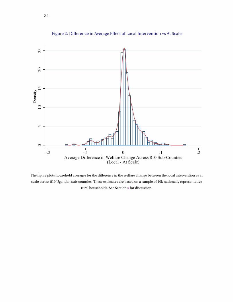
34

Figure 2: Difference in Average Effect of Local Intervention vs At Scale

05

1015

2025

Den

sity

-.2 -.1 0 .1 .2Average Difference in Welfare Change Across 810 Sub-Counties

(Local - At Scale)

The figure plots household averages for the difference in the welfare change between the local intervention vs at

scale across 810 Ugandan sub-counties. These estimates are based on a sample of 10k nationally representative

rural households. See Section 5 for discussion.

35

Figure 3: Distributional Implications

1.05

1.1

1.15

Cha

nge

in W

elfa

re

0 5 10 15Years of Education of Head of HH

Local At Scale

The figure plots estimates from local polynomial regressions. Shaded areas indicate 95 percent confidence intervals.

See Section 5 for discussion.

36

Figure 4: Comparing 10k Farmers to All Rural Households

1.06

1.07

1.08

1.09

1.1

1.11

Cha

nge

in W

elfa

re

0 5 10 15Years of Education of Head of HH

At Scale--10k Farmers At Scale--All Farmers

At Scale

The figure plots estimates from local polynomial regressions. Shaded areas indicate 95 percent confidence intervals.

See Section 5 for discussion.

37

Figure 5: Pre-Existing Use of Modern Inputs

.06

.08

.1.1

2.1

4Sh

are

Mod

ern

Tech

nolo

gy

0 5 10 15Years of Education of Head of HH

The figure plots estimates from local polynomial regressions. Shaded areas indicate 95 percent confidence intervals.

See Section 5 for discussion.

38

Figure 6: Pre-Existing Shares of Labor Income

.68

.7.7

2.7

4.7

6.7

8Sh

are

of L

abor

Inco

me

0 5 10 15Years of Education of Head of HH

The figure plots estimates from local polynomial regressions. Shaded areas indicate 95 percent confidence intervals.

See Section 5 for discussion.

39

Figure 7: Pre-Existing Expenditure Shares on Agriculture

.4.4

5.5

.55

.6.6

5Sh

are

of F

ood

Expe

nditu

re

0 5 10 15Years of Education of Head of HH

The figure plots estimates from local polynomial regressions. Shaded areas indicate 95 percent confidence intervals.

See Section 5 for discussion.

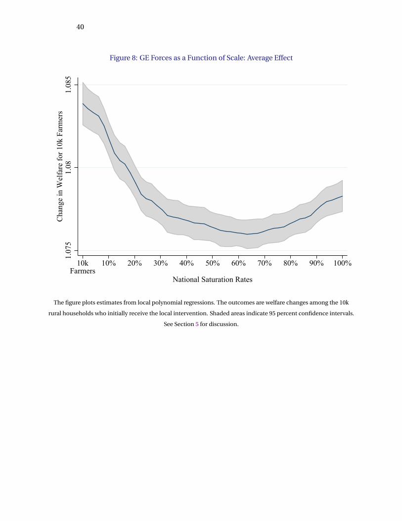
40

Figure 8: GE Forces as a Function of Scale: Average Effect

1.07

51.

081.

085

Cha

nge

in W

elfa

re fo

r 10k

Far

mer

s

10kFarmers

10% 20% 30% 40% 50% 60% 70% 80% 90% 100%

National Saturation Rates

The figure plots estimates from local polynomial regressions. The outcomes are welfare changes among the 10k

rural households who initially receive the local intervention. Shaded areas indicate 95 percent confidence intervals.

See Section 5 for discussion.

41

Figure 9: GE Forces as a Function of Scale: Distribution

.02

.04

.06

.08

Diff

eren

ce in

Wel

fare

Cha

nge

for 1

0k F

arm

ers

Ed

ucat

ed v

s Non

-Edu

cate

d

10kFarmers

10 20 30 40 50 60 70 80 90 100

National Saturation Rates in %

The figure plots point estimates from regressions of welfare changes (LHS) on a dummy for heads of households

with 10 or more years of education (RHS) among the 10k of rural households who initially receive the local

intervention. The reference category are households without any years of education (roughly 25% of rural

households). Point estimates are estimated in separate regressions with counterfactual welfare changes solved for

different levels of national saturation. Shaded areas indicate 95 percent confidence intervals. See Section 5 for

discussion.

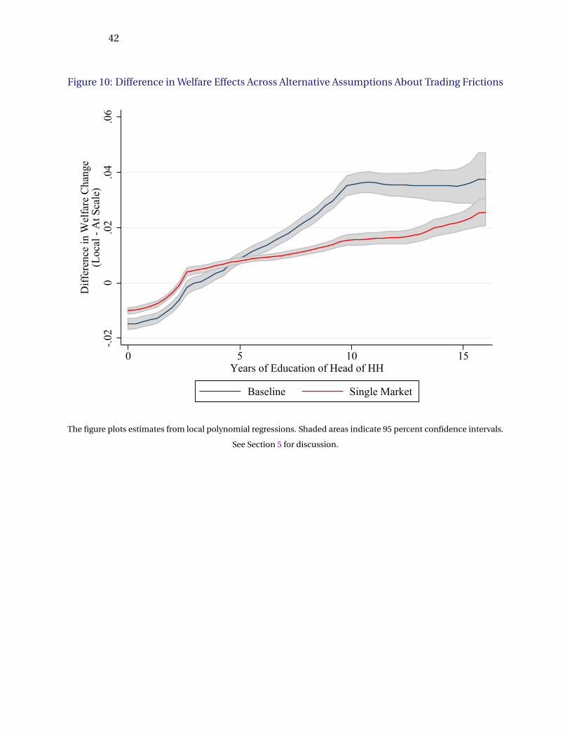
42

Figure 10: Difference in Welfare Effects Across Alternative Assumptions About Trading Frictions

-.02

0.0

2.0

4.0

6

Diff

eren

ce in

Wel

fare

Cha

nge

(Loc

al -

At S

cale

)

0 5 10 15Years of Education of Head of HH

Baseline Single Market

The figure plots estimates from local polynomial regressions. Shaded areas indicate 95 percent confidence intervals.

See Section 5 for discussion.

43

Figure 11: Differences in Welfare Effects as a Function of Pre-Existing Exporting

-.02

0.0

2.0

4.0

6

Diff

eren

ce in

Wel

fare

Cha

nge

(Loc

al -

At S

cale

)

0 5 10 15Years of Education of Head of HH

Above Median Export Share Below Median Export Share

The figure plots estimates from local polynomial regressions. Shaded areas indicate 95 percent confidence intervals.

See Section 5 for discussion.

44

Figure 12: Difference in Welfare Effects Across Alternative Levels of Aggregation

-.02

0.0

2.0

4.0

6.0

8

Diff

eren

ce in

Wel

fare

Cha

nge

(Loc

al -

At S

cale

)

0 5 10 15Years of Education of Head of HH

Baseline District-Level Aggregation

The figure plots estimates from local polynomial regressions. Shaded areas indicate 95 percent confidence intervals.

See Section 5 for discussion.

45

Figure 13: Results Across Alternative Parameter Assumptions: Kappas

Panel A

1.05

1.1

1.15

Cha

nge

in W

elfa

re

0 5 10 15Years of Education of Head of HH

Kappa=1.3 Kappa=1.8 (Baseline) Kappa=2.8

At Scale

Panel B: Differences in Welfare Effect (Local-At Scale)

-.1-.0

50

.05

Diff

eren

ce in

Wel

fare

Cha

nge

(At S

cale

-Loc

al)

0 5 10 15Years of Education of Head of HH

Kappa=1.3 Kappa=1.8 (Baseline) Kappa=2.8

The figure plots estimates from local polynomial regressions. Shaded areas indicate 95 percent confidence intervals.

See Section 5 for discussion.

46

Figure 14: Results Across Alternative Parameter Assumptions: Sigmas

Panel A

1.06

1.07

1.08

1.09

1.1

1.11

Cha

nge

in W

elfa

re

0 5 10 15Years of Education of Head of HH

Sigma=2.6 (Baseline) Sigma=3.6 Sigma=4.6

At Scale

Panel B: Differences in Welfare Effect (Local - At Scale)

-.06

-.04

-.02

0.0

2

Diff

eren

ce in

Wel

fare

Cha

nge

(At S

cale

-Loc

al)

0 5 10 15Years of Education of Head of HH

Sigma=2.6 (Baseline) Sigma=3.6 Sigma=4.6

The figure plots estimates from local polynomial regressions. Shaded areas indicate 95 percent confidence intervals.

See Section 5 for discussion.

47

Figure 15: Model Validation Using Cross-Sectional Moments: Market Prices

-.4-.3

-.2-.1

0.1

.2.3

Pred

icte

d D

evia

tins i

n Lo

g Pr

ices

-.5 -.4 -.3 -.2 -.1 0 .1 .2 .3 .4Observed Deviations in Log Prices (Trader Surveys)

The figure plots estimates from local polynomial regressions. Both y and x-axes are deviations relative to

crop-by-time fixed effects. Shaded areas indicate 95 percent confidence intervals. See Section 5 for discussion.

48

Figure 16: Road Addition in 2003 as a Natural Experiment for Model Validation

The map displays road additions over the period 2000-2013. See Section 5 for discussion.

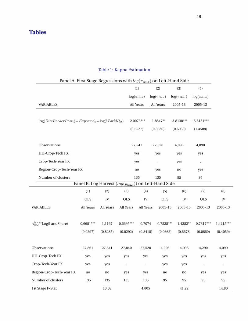
49

Tables

Table 1: Kappa Estimation

Panel A: First Stage Regressions with log(πikωt) on Left-Hand Side

(1) (2) (3) (4)

log(πikωt) log(πikωt) log(πikωt) log(πikωt)

VARIABLES All Years All Years 2005-13 2005-13

log(DistBorderPosti) ∗ Exportedk ∗ log(WorldPkt) -2.0073*** -1.8547** -3.8138*** -5.6151***

(0.5527) (0.8636) (0.6060) (1.4508)

Observations 27,541 27,520 4,096 4,090

HH-Crop-Tech FX yes yes yes yes

Crop-Tech-Year FX yes . yes .

Region-Crop-Tech-Year FX no yes no yes

Number of clusters 135 135 95 95

Panel B: Log Harvest (log(yikωt)) on Left-Hand Side

(1) (2) (3) (4) (5) (6) (7) (8)

OLS IV OLS IV OLS IV OLS IV

VARIABLES All Years All Years All Years All Years 2005-13 2005-13 2005-13 2005-13

αlandikω *Log(LandShare) 0.6681*** 1.1167 0.6695*** 0.7074 0.7525*** 1.4252** 0.7817*** 1.4215***

(0.0297) (0.8285) (0.0292) (0.8418) (0.0662) (0.6678) (0.0660) (0.4059)

Observations 27,861 27,541 27,840 27,520 4,296 4,096 4,290 4,090

HH-Crop-Tech FX yes yes yes yes yes yes yes yes

Crop-Tech-Year FX yes yes . . yes yes . .

Region-Crop-Tech-Year FX no no yes yes no no yes yes

Number of clusters 135 135 135 135 95 95 95 95

1st Stage F-Stat 13.09 4.805 41.22 14.80

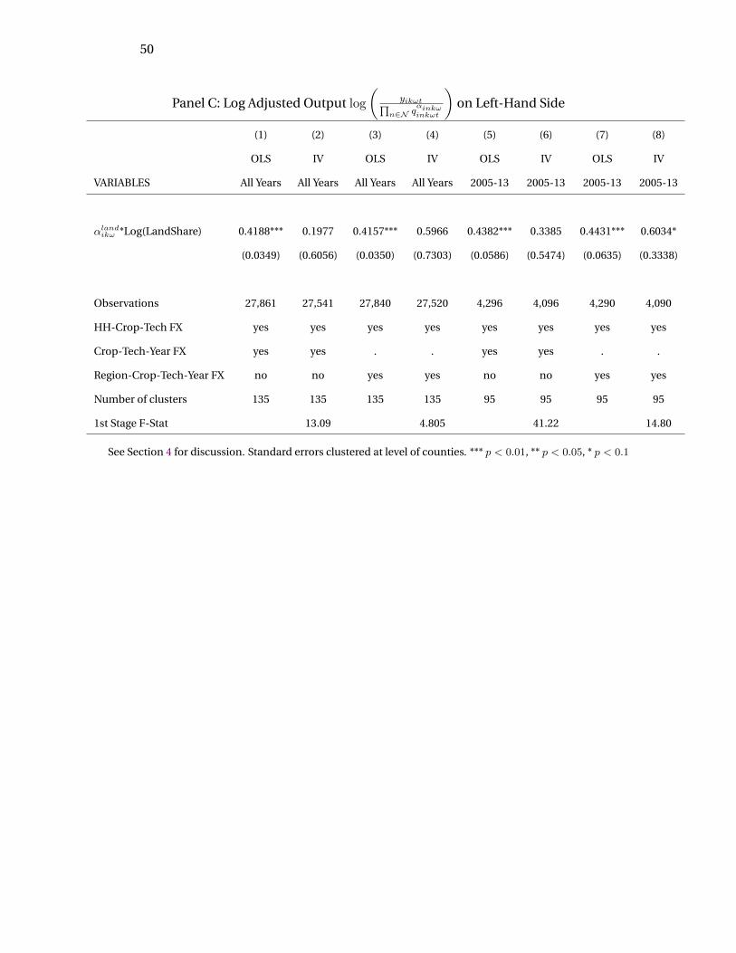
50

Panel C: Log Adjusted Output log

(yikωt∏

n∈N qαinkωinkωt

)on Left-Hand Side

(1) (2) (3) (4) (5) (6) (7) (8)

OLS IV OLS IV OLS IV OLS IV

VARIABLES All Years All Years All Years All Years 2005-13 2005-13 2005-13 2005-13

αlandikω *Log(LandShare) 0.4188*** 0.1977 0.4157*** 0.5966 0.4382*** 0.3385 0.4431*** 0.6034*

(0.0349) (0.6056) (0.0350) (0.7303) (0.0586) (0.5474) (0.0635) (0.3338)

Observations 27,861 27,541 27,840 27,520 4,296 4,096 4,290 4,090

HH-Crop-Tech FX yes yes yes yes yes yes yes yes

Crop-Tech-Year FX yes yes . . yes yes . .

Region-Crop-Tech-Year FX no no yes yes no no yes yes

Number of clusters 135 135 135 135 95 95 95 95

1st Stage F-Stat 13.09 4.805 41.22 14.80

See Section 4 for discussion. Standard errors clustered at level of counties. *** p < 0.01, ** p < 0.05, * p < 0.1

51

Table 2: Effect on Household Welfare

(1) (2)

Welfare Welfare

VARIABLES Local At Scale

Hat Change 1.0847*** 1.0787***

(0.0011) (0.0009)

Observations 10,000 10,000

No Clusters 3731 3731

Standard errors clustered at market-level.

*** p<0.01, ** p<0.05, * p<0.1The table presents effects from the local and from the intervention at scale for the identical representative sample of

10k randomly selected rural households. See Section 5 for discussion.

52

Table 3: Effects on Incomes and Prices

Panel A(1) (2) (3) (4) (5) (6) (7) (8) (9) (10) (11) (12)

Income Wage P manu P banana P bean P cassava P coffee P groundnut P maize P millet P sorghum P sweetpot

VARIABLES Local Local Local Local Local Local Local Local Local Local Local Local

Effect 1.0790*** 1.0117*** 1.0000 1.0003*** 0.9933*** 0.9909*** 1.0000 0.9993*** 0.9906*** 1.0001*** 0.9994*** 0.9992***

(0.0011) (0.0004) (0.0000) (0.0000) (0.0002) (0.0003) (0.0000) (0.0001) (0.0003) (0.0000) (0.0001) (0.0001)

Observations 10,000 10,000 10,000 10,000 10,000 10,000 10,000 10,000 10,000 10,000 10,000 10,000

No Clusters 3731 3731 3731 3731 3731 3731 3731 3731 3731 3731 3731 3731

Panel B(1) (2) (3) (4) (5) (6) (7) (8) (9) (10) (11) (12)

Income Wage P manu P banana P bean P cassava P coffee P groundnut P maize P millet P sorghum P sweetpot

VARIABLES At Scale At Scale At Scale At Scale At Scale At Scale At Scale At Scale At Scale At Scale At Scale At Scale

Effect 1.0683*** 1.0671*** 1.0000 1.0031*** 0.9568*** 0.9794*** 0.9985*** 0.9750*** 0.9719*** 1.0282*** 0.9970*** 1.0087***

(0.0010) (0.0012) (0.0000) (0.0001) (0.0004) (0.0007) (0.0001) (0.0004) (0.0004) (0.0003) (0.0001) (0.0004)

Observations 10,000 10,000 10,000 10,000 10,000 10,000 10,000 10,000 10,000 10,000 10,000 10,000

No Clusters 3731 3731 3731 3731 3731 3731 3731 3731 3731 3731 3731 3731

Standard errors clustered at market-level.

*** p<0.01, ** p<0.05, * p<0.1

The table presents effects from the local and from the intervention at scale for the identical representative sample of 10k rural households. See

Section 5 for discussion.

53

Table 4: Effect on Rural vs Urban Households

(1) (2) (3) (4)

Welfare Welfare Welfare Welfare

Local Local At Scale At Scale

VARIABLES 10k Farmers Urban HHs 10k Farmers Urban HHs

Hat Change 1.0847*** 1.0000 1.0787*** 1.0082***

(0.0011) (0.0000) (0.0009) (0.0005)

Observations 10,000 70 10,000 70

No Clusters 3731 3731

Standard errors clustered at market-level.

*** p<0.01, ** p<0.05, * p<0.1Urban households are aggregated as representative agents across 70 cities. See Section 5 for discussion.

54

Table 5: Reduced-Form Evidence from Road Building

(1) (2) (3) (4)

VARIABLES Log Total Outlays Log Total Outlays Log Land Log Land

Beans*logMA -1.3318*** -1.3049**

(0.4534) (0.5429)

Cassava*logMA 0.9325*** 0.2430

(0.2526) (0.4371)

Millet*logMA 1.4664*** 1.5100**

(0.5048) (0.7126)

Maize*logMA -0.2183 -0.5949

(0.7370) (0.5601)

Sorghum*logMA 0.9958 -1.2796***

(1.0425) (0.4813)

SweetPot*logMA -2.8033*** -2.5430***

(0.6914) (0.5206)

log(Market Access) 0.5893*** 0.9053***

(0.1804) (0.1681)

Observations 3,434 3,432 6,958 6,922

R-squared 0.7605 0.7892 0.6675 0.7134

HH FX yes yes . .

Year FX yes . . .

District-Year FX no yes . .

HH-Crop-Tech FX . . yes yes

Crop-Tech-Year FX . . yes .

District-Crop-Tech-Year FX . . no yes

Number of clusters 256 255 250 250

See Section 5 for discussion. Log Total Outlays are based on annualized household consumption expenditure per

capita. Log Land is land area in acres used for the production of each crop. The regression uses the UNPS microdata

for 2005 and 2009 to test for the effects of a road addition in 2003 (see map in Figure 16). The regression sample

excludes parishes in the UNPS data directly affected by the new road. Banana, coffee and groundnuts are excluded

as those crops are not grown in the region of the road addition. Standard errors are clustered at the level of parishes.

55

Table 6: Reduced-Form Evidence from Weather Shocks

(1) (2) (3)

VARIABLES Log Total Outlays Log Harvest Log Land

Cereals*HotDays -0.0167 -0.0149*

(0.0111) (0.0083)

Tubers*HotDays -0.0056 -0.0073

(0.0072) (0.0081)

Other*HotDays -0.0056 -0.0131*

(0.0083) (0.0070)

Cereals*logRain 0.3856*** 0.2551***

(0.0903) (0.0803)

Tubers*logRain -0.7561*** -0.1996***

(0.0461) (0.0491)

Other*logRain 0.3954*** 0.2557***

(0.0369) (0.0386)

HotDays 0.0030

(0.0034)

log(RainFall) 0.6258***

(0.0174)

Observations 8,988 31,478 31,478

R-squared 0.7124 0.7245 0.6045

HH FX yes . .

Year FX yes . .

HH-Crop-Tech FX . yes yes

Crop-Tech-Year FX . yes yes

Number of clusters 381 380 380

See Section 5 for discussion. Log Total Outlays are based on annualized household consumption expenditure per

capita. Log Land is land area in acres used for the production of each crop. Log Harvest is the amount of crop

harvest measured in kg. HotDays and logRainfall are the number of days above 29 degrees Celsius and the total

amount of rainfall recorded during growing seasons per year. Standard errors are clustered at the level of parishes.

1

8 Appendix

Appendix 1: Additional Figures and Tables

Table A.1: Main Crops

(1) (2)

Aggregate Median

VARIABLES Share of Land Share of Land

cropID==Beans 0.1442 0.1072

(0.0086) (0.0078)

cropID==Cassava 0.1908 0.0917

(0.0121) (0.0063)

cropID==Coffee 0.0718 0.0000

(0.0048) (0.0000)

cropID==Groundnuts 0.0541 0.0000

(0.0052) (0.0000)

cropID==Maize 0.1723 0.0923

(0.0119) (0.0052)

cropID==Matooke 0.1646 0.0089

(0.0040) (0.0089)

cropID==Millet 0.0315 0.0000

(0.0021) (0.0000)

cropID==Sorghum 0.0524 0.0000

(0.0037) (0.0000)

cropID==Sweet Potatoes 0.0886 0.0259

(0.0061) (0.0070)

Observations 45 45

Total Share .859 .986

*** p<0.01, ** p<0.05, * p<0.1

Aggregate and median shares for each of the 9 crops are computed for each of four years of data from the UNPS. The

table reports the means and standard deviations across the 4 rounds of data. See Section 2 for discussion of the data.

2

Figure A.1: Regional Specialization

The figure displays the crop with the highest land allocation in each Ugandan district. We use the UNPS data to

compute the mean of each crop’s land shares across 4 rounds of data. See Section 2 for discussion of the data.

3

Table A.2: Regional Price Gaps

See Section 2 for discussion of the data.

4

Table A.3: Farmer Trading vs Subsistence

Panel A

Panel B

See Section 2 for discussion of the data.

5

Table A.4: Farmers Sell Their Crops to Local Markets

Selling Mode Count in 1000 Share

Government/LC 285.8 0.00400

Private trader in local village/market 44269 0.672

Private trader in district market 7081 0.107

Consumer at market 9744 0.148

Neighbor/ Relative 3907 0.0590

Other (specify) 610.6 0.00900

Total 65898 1See Section 2 for discussion of the data.

6

Table A.5: Farmers Re-Allocate Their Land Across Crops Over Time

Panel A

Panel B

See Section 2 for discussion of the data.

7

Table A.6: Product Differentiation (Missing Trade Flows

(1) (2)

VARIABLES Buying Dummy Selling Dummy

Proportion Trading 0.0429*** 0.0432***

(0.0021) (0.0021)

Observations 9,146 9,146

*** p<0.01, ** p<0.05, * p<0.1See Section 2 for discussion of the data.

Figure A.2: Household Preferences (Non-Homotheticity)

.2.3

.4.5

.6Sh

are

of F

ood

Expe

nditu

re

-2 -1 0 1 2Deviations of Log Total Expenditure Per Capita

See Section 2 for discussion of the data.

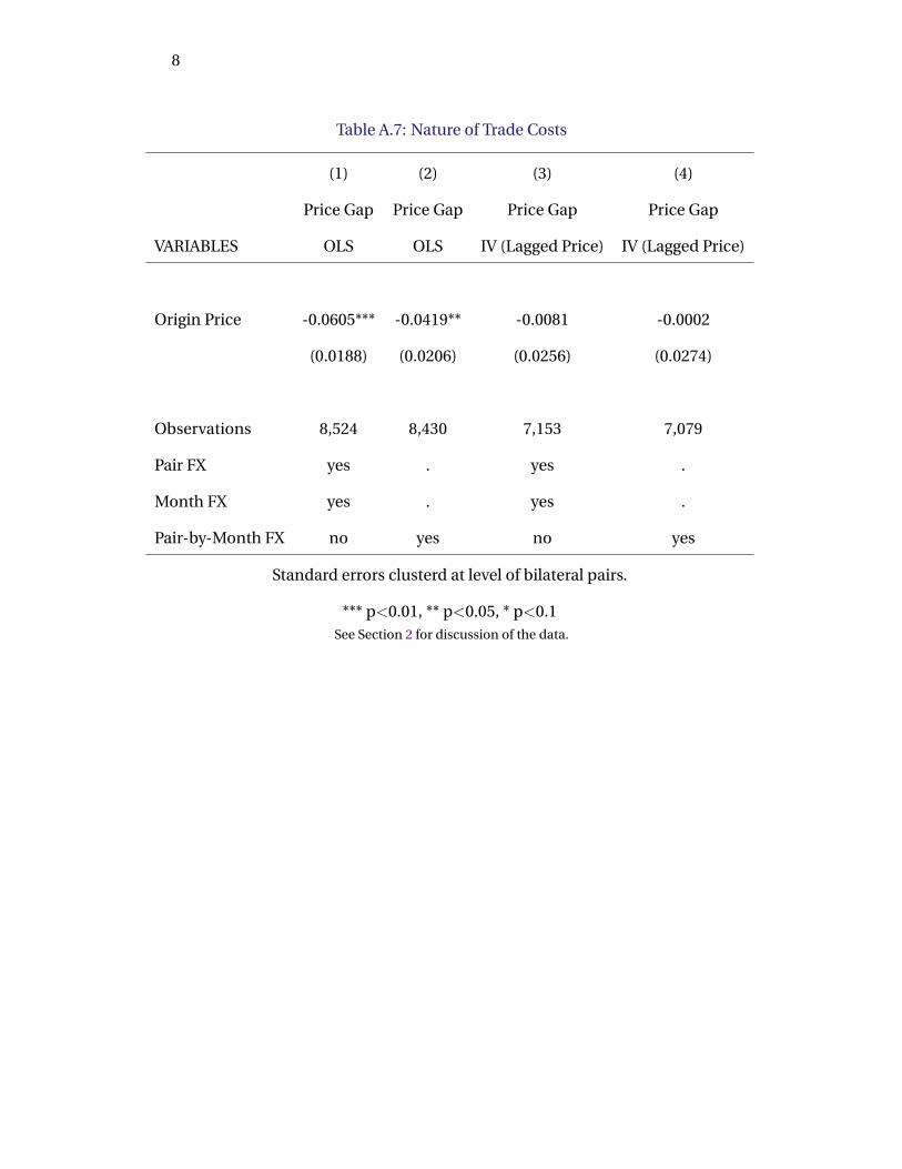
8

Table A.7: Nature of Trade Costs

(1) (2) (3) (4)

Price Gap Price Gap Price Gap Price Gap

VARIABLES OLS OLS IV (Lagged Price) IV (Lagged Price)

Origin Price -0.0605*** -0.0419** -0.0081 -0.0002

(0.0188) (0.0206) (0.0256) (0.0274)

Observations 8,524 8,430 7,153 7,079

Pair FX yes . yes .

Month FX yes . yes .

Pair-by-Month FX no yes no yes

Standard errors clusterd at level of bilateral pairs.

*** p<0.01, ** p<0.05, * p<0.1See Section 2 for discussion of the data.

9

Table A.8: Technology Adoption and Production Cost Shares

(1) (2)

VARIABLES Labor Share Labor Share

Use Modern 0.1056*** 0.0423***

(0.0126) (0.0112)

Observations 26,037 25,889

District FX yes .

Crop FX yes yes

Season FX yes yes

Farmer FX no yes

Standard errors clusterd at level of farmers.

*** p<0.01, ** p<0.05, * p<0.1See Section 2 for discussion of the data.

10

Table A.9: Calibrated Cost Shares in Production

(1) (2) (3) (4) (5) (6)

Land Share Labor Share Intermediate Share Land Share Labor Share Intermediate Share

VARIABLES Traditional Traditional Traditional Modern Modern Modern

cropID1==Beans 0.5107 0.4893 0.0000 0.4607 0.3852 0.1541

(0.0259) (0.0259) (0.0000) (0.0041) (0.0139) (0.0154)

cropID1==Cassava 0.5566 0.4434 0.0000 0.4429 0.3785 0.1786

(0.0503) (0.0503) (0.0000) (0.0180) (0.0187) (0.0176)

cropID1==Coffee 0.6777 0.3223 0.0000 0.5428 0.2683 0.1889

(0.0571) (0.0571) (0.0000) (0.0164) (0.0202) (0.0122)

cropID1==Groundnuts 0.5134 0.4866 0.0000 0.4204 0.4253 0.1543

(0.0231) (0.0231) (0.0000) (0.0190) (0.0450) (0.0271)

cropID1==Maize 0.5000 0.5000 0.0000 0.4153 0.4335 0.1512

(0.0272) (0.0272) (0.0000) (0.0520) (0.0559) (0.0159)

cropID1==Matooke 0.6343 0.3657 0.0000 0.6180 0.2564 0.1256

(0.0455) (0.0455) (0.0000) (0.0394) (0.0275) (0.0119)

cropID1==Millet 0.5285 0.4715 0.0000 0.5485 0.3381 0.1134

(0.0174) (0.0174) (0.0000) (0.0074) (0.0039) (0.0035)

cropID1==Sorghum 0.5563 0.4437 0.0000 0.5774 0.3321 0.0905

(0.0216) (0.0216) (0.0000) (0.0062) (0.0060) (0.0051)

cropID1==Sweet Potatoes 0.5088 0.4912 0.0000 0.4721 0.3642 0.1637

(0.0258) (0.0258) (0.0000) (0.0735) (0.0800) (0.0107)

See Section 4 for discussion and Section 2 for description of the data.

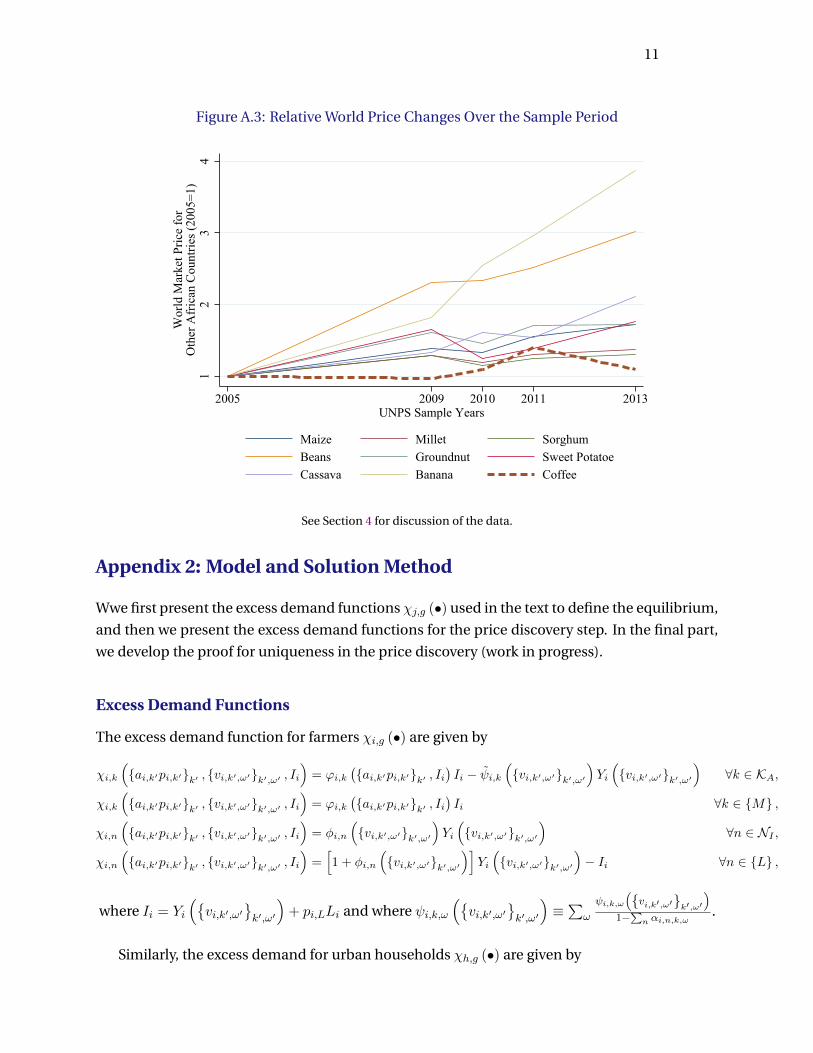
11

Figure A.3: Relative World Price Changes Over the Sample Period

12

34

Wor

ld M

arke

t Pric

e fo

rO

ther

Afr

ican

Cou

ntrie

s (20

05=1

)

2005 2009 2010 2011 2013UNPS Sample Years

Maize Millet SorghumBeans Groundnut Sweet PotatoeCassava Banana Coffee

See Section 4 for discussion of the data.

Appendix 2: Model and Solution Method

Wwe first present the excess demand functions χj,g (•) used in the text to define the equilibrium,

and then we present the excess demand functions for the price discovery step. In the final part,

we develop the proof for uniqueness in the price discovery (work in progress).

Excess Demand Functions

The excess demand function for farmers χi,g (•) are given by

χi,k

(ai,k′pi,k′k′ , vi,k′,ω′k′,ω′ , Ii

)= ϕi,k

(ai,k′pi,k′k′ , Ii

)Ii − ψi,k

(vi,k′,ω′k′,ω′

)Yi

(vi,k′,ω′k′,ω′

)∀k ∈ KA,

χi,k

(ai,k′pi,k′k′ , vi,k′,ω′k′,ω′ , Ii

)= ϕi,k

(ai,k′pi,k′k′ , Ii

)Ii ∀k ∈ M ,

χi,n

(ai,k′pi,k′k′ , vi,k′,ω′k′,ω′ , Ii

)= φi,n

(vi,k′,ω′k′,ω′

)Yi

(vi,k′,ω′k′,ω′

)∀n ∈ NI ,

χi,n

(ai,k′pi,k′k′ , vi,k′,ω′k′,ω′ , Ii

)=[1 + φi,n

(vi,k′,ω′k′,ω′

)]Yi

(vi,k′,ω′k′,ω′

)− Ii ∀n ∈ L ,

where Ii = Yi

(vi,k′,ω′

k′,ω′

)+ pi,LLi and where ψi,k,ω

(vi,k′,ω′

k′,ω′

)≡∑

ω

ψi,k,ω

(vi,k′,ω′k′,ω′

)1−∑n αi,n,k,ω

.

Similarly, the excess demand for urban households χh,g (•) are given by

12

χh,k

(ah,k′ph,k′

k′,vh,k′,ω′

k′,ω′

, Ih

)= ϕh,k

(ah,k′ph,k′

k′, Ih)Ih ∀k ∈ KA,

χh,k

(ah,k′ph,k′

k′,vh,k′,ω′

k′,ω′

, Ih

)=[ϕh,k

(ah,k′ph,k′

k′, Ih)− 1]Ih ∀k ∈ M ,

χh,k

(ah,k′ph,k′

k′,vh,k′,ω′

k′,ω′

, Ih

)= 0 ∀n ∈ NI .

where Ih = bh,Mph,MLh.1,2Finally, forForeignwehaveχF,g =

−∞ if pF,g < p∗F,g

]−∞,∞[ if pF,g = p∗F,g

∞ if pF,g > p∗F,g

.

Excess demand as functions of data D and prices pj,g for farmers and

urban households (used for the price discovery step) are given by

χi,k

(pi,gg ;D

)= ξi,kIi −

∑ω

pi,kyi,k,ω ∀k ∈ KA,

χi,k

(pi,gg ;D

)= ξi,kIi ∀k ∈ M ,

χi,n

(pi,gg ;D

)=∑k,ω

αi,n,k,ωpi,kyi,k,ω ∀n ∈ NI ,

χi,n

(pi,gg ;D

)=∑k,ω

αi,n,k,ωpi,kyi,k,ω − pi,nLi ∀n ∈ L ,

χh,k

(ph,gg ;D

)= ξh,kIh ∀k ∈ KA,

χh,k

(ph,gg ;D

)= (ξh,k − 1) Ih ∀k ∈ M ,

χh,n

(ph,gg ;D

)= 0 ∀n ∈ NI ,

χF,g

(pj,gg ;D

)=

−∞ if pF,g < p∗F,g

]−∞,∞[ if pF,g = p∗F,g

∞ if pF,g > p∗F,g

∀g,

1We include vh,k′,ω′k′,ω′ as an argument in χh,k(•) so that χj,g(aj,kpj,kk , vj,k,ωk,ω , Ij

)capture urban

households – since the function does not depend on these arguments, there is no need to define them.2In parallel to our treatment of land for farmers, we assume that there is no market for household labor in urban

areas, and hence the equilibrium system does not have to determine the price of this good.

13

where

Ii

(pi,gg ;D

)=∑k,ω

(1−

∑n

αi,n,k,ω

)pi,kyi,k,ω + pi,LLi,

Ih

(ph,gg ;D

)= ph,Myh,M .

Price Discovery

In this subsection we show that, in the case with only iceberg trade costs

(i.e., tod,g = 0 for all o, d, g), no inputs and no trade with Foreign, the price

discovery step described in the previous section is well defined in the sense

that there is a unique set of prices pj,g, pm,g that solves the system of

equations 12-14. To do so, we think of that system of equations as charac-

terizing the equilibrium of a competitive exchange economy, and so the goal

is to prove that this economy has a unique equilibrium.

We consider an equivalent economy where there is a single market with

an expanded set of goods (which we now call varieties) given by

V ≡ (o, g) ∈ J ×K | yo,g > 0 .

A variety of good g produced by agent o is indexed by (o, g) ∈ J × K.

Agent o′s endowment of (o, g) is yo,g. Naturally, no other agent o′ 6= o has

a positive endowment of (o, g) and so yo,g is also the total endowment of

variety (o, g) in the economy.

Next, we let τod,g be the minimum cost at which variety (o, g) can be

transported from its origin to destination d.3 Letting po,g denote the price

of variety (o, g) ∈ V , we know that in a competitive equilibrium the price

of a variety must be equal to its cost, and hence the price at which agent d

has access to variety (o, g) is τod,gpo,g.

We let ξd,g ∈ [0, 1] denote the expenditure share of gross income of agent

d (i.e.,∑

g∈K pd,gyd,g) on good g. The excess demand function (in quantities)

3Formally,τod,g ≡ min

φ∈Φod,g

∏(o′,d′)∈φ

τo′d′,g,

where Φod,g is the set of directed walks from o to d for good g and each element φ ∈ Φod,gis a sequence of edges (on, dn)Nn=1 such that o1 = o, dN = d, and on+1 = dn.

14

for a variety (o, g) ∈ V is given by

χo,g (p) =∑d

χd,o,g (p)− yo,g,

where p ≡ po,g(o,g)∈V and χd,o,g (•) is the demand function of agent d for

variety (o, g) and is given by

χd,o,g (p) ∈

[0,

ξd,gpo,g τod,g

Id

]if o ∈ arg mino′∈J po′,g τo′d,g

0 if o /∈ arg mino′∈J po′,g τo′d,g

,

Id =∑g

pd,gyd,g.

In what follows, we follow the convention that yo,g = 0 =⇒ po,g =∞.

The equilibrium is a set of prices p such that the excess demand for all

varieties in V is zero,

χo,g (p) = 0∀ (o, g) ∈ V. (1)

(Endowments and demand.)

1.∑

g∈K yo,g > 0∀o ∈ J .

2. yd,g > 0 =⇒ ξd,g > 0∀d ∈ J , g ∈ K.

A price vector p is strongly connected if there is no partition J0,J1 of

J such that for all g ∈ K, χd,o,g (p) = χo,d,g (p) = 0∀o ∈ J0, d ∈ J1. Given

Assumption 1, there can be at most one strongly connected price vector p

– up to the choice of numeraire – that solves the system of equations

p′o,g = po,g∀(o, g) ∈M0,

p′o,g > po,g∀(o, g) ∈M1,

where M0 6= ∅ and M1 6= ∅. Focusing on such prices (p,p′), we show a

contradiction by way of five claims.

Before stating the claims, we introduce some additional definitions and

notation. Given (p,p′), consider the set of partitionsO∗−1,g,O∗0,g,O∗1,g

g∈K

15

of J such that

yo,g = 0∀o ∈ O∗−1,g,

p′o,g = po,g∀o ∈ O∗0,g,

p′o,g > po,g∀o ∈ O∗1,g,

the set of partitions G−1,d,G0,d,G1,dd∈J of K such that

ξd,g = 0∀g ∈ G−1,d,

ξd,g > 0 ∧

arg mino∈J

po,g τod,g

∩ O∗0,g 6= ∅∀g ∈ G0,d,

ξd,g > 0 ∧

arg mino∈J

po,g τod,g

∩ O∗0,g = ∅∀g ∈ G1,d,

the set of partitionsD∗−1,g,D∗0,g,D∗1,g

g∈K of J such that

g ∈ G−1,d∀d ∈ D∗−1,g,

g ∈ G0,d∀d ∈ D∗0,g,

g ∈ G1,d∀d ∈ D∗1,g,

and finally the partition J−,J+,J± of J such that

G1,d = ∅∀d ∈ J−,

G0,d = ∅∀d ∈ J+,

G0,d 6= ∅ ∧ G1,d 6= ∅∀d ∈ J±.

In words, O∗−1,g is the set of agents who have a zero endowment of good

g while O∗0,g (O∗1,g) is the set of agents o for which their variety of good

g does not change (increases in) price; G−1,d is the set of goods for which

expenditure is zero for agent d while G0,d (G1,d) is the set of goods whose

price (inclusive of trade cost) does not increase (increases) for agent d; D∗−1,g

is the set of agents who have zero expenditure on good g while D∗0,g (D∗1,g) is

the set of agents who do not (do) face an increase in price of good g; and J−(J+) is the set of agents for whom the price of all goods remains the same

(increases) and J± is the set of agents that for whom some goods increase

in price while others do not. Note that we could have equivalently defined

16

J− ≡ ∩gD∗0,g and J+ ≡ ∩gD∗1,g,with J± ≡ J\ (J− ∪ J+).

For all g ∈ K,

χd,o,g (p) = 0∀o ∈ J−, d ∈ J+,

χd,o,g (p) = 0∀o ∈ J+, d ∈ J−.

For any d ∈ J+, G0,d = ∅. Hence, for all d ∈ J+ and g ∈ K\G−1,d, it

must be the case that ∃o ∈ O∗1,g such that χd,o,g (p) > 0 while χd,o,g (p) =

0∀o /∈ O∗1,g. Further, it follows from the definition of J− and the fact that in

equilibrium an agent always consumes a positive amount of its own varieties

(from Assumption 1, yd,g > 0 =⇒ ξd,g > 0) that J−∩(∪g∈KO∗1,g

)= ∅. This

implies that agents in J+ purchase no positive value from agents in J− under

equilibrium prices p, that is, for all g ∈ K, χd,o,g (p) = 0∀o ∈ J−, d ∈ J+.

Similarly, for any d ∈ J−, G1,d = ∅. Hence, for all d ∈ J− and g ∈

K\G−1,d, it must be the case that ∃o ∈ O∗0,g such that χd,o,g (p) > 0 while

χd,o,g (p) = 0∀o /∈ O∗0,g. Since J+∩(∪g∈KO∗0,g

)= ∅, this implies that agents

in J− purchase no positive value from agents in J+ under equilibrium prices

p, that is, for all g ∈ K, χd,o,g (p) = 0∀o ∈ J+, d ∈ J−. J± 6= ∅. Suppose

J± = ∅. Then J−,J+ form a partition of J and then Claim 1 implies

that p is not strongly connected, leading to a contradiction.

J± ∩(∪g∈KO∗1,g

)6= ∅. In words, there is a least one agent for whom the

prices of some goods increase and the prices of others do not while at the

same time experiencing an increase in the price of it’s variety of at least one

good. We consider two cases.

J+ = ∅.

Since M1 6= ∅, then ∪g∈KO∗1,g 6= ∅, and so J ∩(∪g∈KO∗1,g

)6= ∅. Then,

J ∩(∪g∈KO∗1,g

)6= ∅

=⇒(J− ∩

(∪g∈KO∗1,g

))∪(J± ∩

(∪g∈KO∗1,g

))6= ∅

=⇒ J± ∩(∪g∈KO∗1,g

)6= ∅,

where the second line follows from the fact that, since J+ = ∅, then J− ∪

J± = J , and the last line follows from the fact that J− ∩(∪g∈KO∗1,g

)= ∅.

J+ 6= ∅.

17

We proceed by contradiction. Suppose J± ∩(∪g∈KO∗1,g

)= ∅. From

Claim 2, we know that J± 6= ∅. For any d ∈ J± , G1,d 6= ∅. Hence, for all

d ∈ J±, ∃ g ∈ K and o ∈ O∗1,g such that χd,o,g (p) > 0. In other words, for a

good whose price increased for d ∈ J±, it must come (in the equilibrium with

p) from an agent for whom the price of that variety increased. Further, note

that for all g ∈ K, O∗1,g ⊆ D∗1,g (from part 2 of Assumption 1). Since J± ∪

J+ = ∪g∈KD∗1,g and J± ∩(∪g∈KO∗1,g

)= ∅, it then follows that ∪g∈KO∗1,g ⊆

J+. This implies that if an agent o ∈ O∗1,g for any g ∈ K, it must also be

the case that o ∈ J+. Hence, for all agents d ∈ J±, ∃g ∈ K and o ∈ J+ such

that χd,o,g (p) > 0. This implies that agents in J± must purchase a positive

value from agents in J+ under equilibrium prices p, that is,

∑o∈J+

∑d∈J±

∑g∈K

po,g τod,gχd,o,g (p) > 0.

For any d ∈ J+, G0,d = ∅. Hence, for all d ∈ J+ and g ∈ K\G−1,d, it must

be the case that ∃o ∈ O∗1,g such that χd,o,g (p) > 0 and for all o /∈ O∗1,g,

χd,o,g (p) = 0. Since J± ∩(∪g∈KO∗1,g

)= ∅, this implies that agents in J+

purchase no positive value from agents in J± under equilibrium prices p,

that is,

∑o∈J±

∑d∈J+

∑g∈K

po,g τod,gχd,o,g (p) = 0.

From Claim 1, it also follows that

∑o∈J−

∑d∈J+

∑g∈K

po,g τod,gχd,o,g (p) = 0,

∑o∈J+

∑d∈J−

∑g∈K

po,g τod,gχd,o,g (p) = 0.

Since the budget constraint of an agent o ∈ J+ is satisfied with equality

under equilibrium prices p, we have

∑g∈K

∑d∈J

po,g τod,gχd,o,g (p) =∑g∈K

∑o′∈J

po′,g τo′o,gχo,o′,g (p)∀o ∈ J+

18

and hence

∑g∈K

∑d∈J±

po,g τod,gχd,o,g (p)

+∑g∈K

∑d∈J−

po,g τod,gχd,o,g (p)

+∑g∈K

∑d∈J+

po,g τod,gχd,o,g (p) =∑g∈K

∑o′∈J±

po′,g τo′o,gχo,o′,g (p)

+∑g∈K

∑o′∈J−

po′,g τo′o,gχo,o′,g (p)

+∑g∈K

∑o′∈J+

po′,g τo′o,gχo,o′,g (p) ∀o ∈ J+

=⇒∑o∈J+

∑g∈K

∑d∈J±

po,g τod,gχd,o,g (p)

+∑o∈J+

∑g∈K

∑d∈J−

po,g τod,gχd,o,g (p)

+∑o∈J+

∑g∈K

∑d∈J+

po,g τod,gχd,o,g (p) =∑d∈J+

∑g∈K

∑o∈J±

po,g τod,gχd,o,g (p)

+∑d∈J+

∑g∈K

∑o∈J−

po,g τod,gχd,o,g (p)

+∑d∈J+

∑g∈K

∑o∈J+

po,g τod,gχd,o,g (p)

=⇒∑o∈J+

∑g∈K

∑d∈J±

po,g τod,gχd,o,g (p)

︸ ︷︷ ︸>0

+∑o∈J+

∑g∈K

∑d∈J−

po,g τod,gχd,o,g (p)

︸ ︷︷ ︸=0

=∑d∈J+

∑g∈K

∑o∈J±

po,g τod,gχd,o,g (p)

︸ ︷︷ ︸=0

+∑d∈J+

∑g∈K

∑o∈J−

po,g τod,gχd,o,g (p)

︸ ︷︷ ︸=0

Clearly, we have reached a contradiction, hence it must be the case that

J±∩(∪g∈KO∗1,g

)6= ∅. LetM0,d ≡

(o, g) ∈M0 | g ∈ G0,d ∧ o ∈

arg mino′ po′gτo′d,g

be the set of varieties consumed by agent d in the equilibrium with prices p

which do not change in price under p′. Then d ∈ J+ ⇐⇒ M0,d = ∅. In

words, an agent experiences an increase in the price of all goods it consumes

19

if and only if this agent was not consuming any variety in the equilibrium

with prices p whose price remained unchanged as we move from p to p′.

Consider an agent d /∈ J+. Then G0,d 6= ∅ and ∀g ∈ G0,d d purchased

good g from an agent o such that (o, g) ∈ M0. We then have M0,d 6= ∅.

The converse follows trivially. Hence d ∈ J+ ⇐⇒ M0,d = ∅. If

χo,g (p) = 0∀ (o, g) ∈ V, then ∃(o, g) ∈V such that χo,g (p′) > 0. Note that

at p (similarly at p′)

χd,o,g (p) =ξd,g

po,g τod,gId,∀(o, g) ∈M0,d,

Id =∑g∈K

pd,gyd,g.

Since M0,d ⊆ M0∀d ∈ J , p′o,g = po,g for all (o, g) ∈ M0,d. It is then clear

that, ∀(o, g) ∈M0,d,

I ′d > Id ⇐⇒ χd,o,g(p′)> χd,o,g (p) ,

I ′d = Id ⇐⇒ χd,o,g(p′)

= χd,o,g (p) .

Further, note that I ′d > Id if ∃g ∈ K such that d ∈ O∗1,g and I ′d = Id if

d /∈ O∗1,g ∀g ∈ K. That is,

d ∈ ∪g∈KO∗1,g =⇒ I ′d > Id,

d /∈ ∪g∈KO∗1,g =⇒ I ′d = Id.

Consequently, we have ∀(o, g) ∈M0,d,

d ∈ ∪g∈KO∗1,g =⇒ χd,o,g(p′)> χd,o,g (p) ,

d /∈ ∪g∈KO∗1,g =⇒ χd,o,g(p′)

= χd,o,g (p) .

Note that for any d ∈ J we have χd,o,g (p′) ≥ χd,o,g (p) = 0∀(o, g) ∈

M0\M0,d.

Next, consider an agent d /∈ J± ∩(∪g∈KO∗1,g

). Then, d ∈ J+ ∪ J− ∪(

J±\(∪g∈KO∗1,g

)). We have three possibilities:

1. Suppose d ∈ J+. From Claim 4, d ∈ J+ =⇒ M0,d = ∅. Therefore,

for d ∈ J+, χd,o,g (p′) = χd,o,g (p)∀(o, g) ∈M0,d vacuously.

20

2. Suppose d ∈ J−. Since J− ∩(∪g∈GO∗1,g

)= ∅ , d /∈ ∪g∈KO∗1,g. There-

fore, for d ∈ J−, χd,o,g (p′) = χd,o,g (p)∀(o, g) ∈M0,d.

3. Suppose d ∈ J±\(∪g∈KO∗1,g

). Clearly d /∈ ∪g∈KO∗1,g . Therefore,

χd,o,g (p′) = χd,o,g (p) ∀(o, g) ∈M0,d, d ∈ J±\(∪g∈KO∗1,g

).

Therefore, for d /∈ J± ∩(∪g∈KO∗1,g

), χd,o,g (p′) = χd,o,g (p) ∀(o, g) ∈M0,d.

Finally, consider an agent d ∈ J± ∩(∪g∈KO∗1,g

)(such an agent exists

thanks to Claim 3). Clearly d ∈ ∪g∈KO∗1,g . Therefore, for d ∈ J± ∩(∪g∈KO∗1,g

), χd,o,g (p′) > χd,o,g (p) ∀(o, g) ∈ M0,d (M0,d 6= ∅ by Claim 4

since d ∈ J± implies d /∈ J+).

Putting these cases together we have

χd,o,g(p′)≥ χd,o,g (p) ∀(o, g) ∈M0\M0,d, d ∈ J ,

χd,o,g(p′)

= χd,o,g (p) ∀(o, g) ∈M0,d, d /∈ J± ∩(∪g∈KO∗1,g

),

χd,o,g(p′)> χd,o,g (p) ∀(o, g) ∈M0,d, d ∈ J± ∩

(∪g∈KO∗1,g

).

Adding across all agents d ∈ J we obtain

χo,g(p′)> χo,g (p)∀(o, g) ∈ ∪d∈J±∩(∪g∈KO∗1,g)M0,d.

Since χo,g (p) = 0∀(o, g) ∈ V, it follows that

χo,g(p′)> 0∀(o, g) ∈ ∪d∈J±∩(∪g∈KO∗1,g)M0,d.

Since J± ∩(∪g∈KO∗1,g

)6= ∅ (from Claim 3) and M0,d 6= ∅∀d ∈ J± ∩(

∪g∈KO∗1,g)

(from Claim 4) imply ∪d∈J±∩(∪g∈KO∗1,g)M0,d 6= ∅, ∃(o, g) ∈ V

such that χo,g (p′) > 0.