- 0 -

Trade Policy, Scale Economies, and Imperfect Competition in Applied Models

March 1996

Joseph F. FrancoisWorld Trade Organization and CEPR

David W. Roland-HolstMills College, OECD Development Centre, and CEPR

I. Introduction

The links between trade policy and competition have received intense scrutiny in recent years.

Current interest in the policy community follows a long period during which many of the basic tenets

of modern industrial organization theory were integrated into the core of mainstream trade theory.

A number of empirical studies of commercial policy have attempted to incorporate theoretical insights

from this literature into numerical assessments of commercial policy. These include studies of regional

integration in North America and Europe (Venables and Smith 1986, 1989; Cox and Harris 1985;

Francois and Shiells 1994), studies of national trade policies (de Melo and Tarr 1992), studies of

multilateral liberalization (Francois et al 1994; Haaland and Tollefson 1994), and sector-focused

commercial policy studies (Dixit 1988; Baldwin and Krugman 1988a,b).

Over roughly the same period during which trade and industrial organization theory were

being integrated, developing countries were grappling with the very real consequences of dramatic

changes in their trade orientation and domestic economic structure. Since 1980, developing countries

have passed through stabilization and adjustment experiences which rival those of the OECD

countries at any time since the second World War. For the most part, closer examination of the

vivid and diverse lessons of this experience by mainstream trade economists has just begun.1 It

- 1 -

is therefore somewhat ironic that the new school of trade theorists has until recently focused its

attention on developed countries, since nowhere has the link between trade and industry structure

and conduct been more apparent in recent times than in developing countries.

In this paper, we examine a variety of alternative specifications of market structure in applied

trade models. After a brief discourse on the concept of procompetitive effects of trade, we turn

to an overview of conventions for specifying scale economies. Following this, we then set out

a menu of specifications for market structure and conduct. While these approaches can be, and

have been, employed in both partial and general equilibrium models, we limit ourselves here to

general equilibrium examples. These examples are drawn from numerical assessments of the Uruguay

Round, under alternative specifications of market structure. For the numerical examples, we work

with a Korea-focused multi-region general equilibrium model.

II. The procompetitive effects of trade policy

When we depart from the perfect competition paradigm, variations in industry structure and market

structure greatly complicate formal analysis of the gains from trade. These complications relate

to potential shifts in the cost of production, rising and falling profit margins, new product

introduction, increased competitive pressure on domestic producers, and changes in the parameters

underlying strategic decisions. The interaction of these effects with trade and trade policy can be

quite complex, though the minimum conditions for welfare gains are generally linked to changes

in industry output. (See Markusen et al, 1995). While the specifics vary my model type, the gains

from trade that are directly linked to conditions of scale economies and/or imperfect competition

are grouped under a common label -- procompetitive effects.

Consider the relatively simple example of procompetitive effects for a small country in which

one sector is monopolistic. This is represented in Figure 1, where sector X is assumed to be

- 2 -

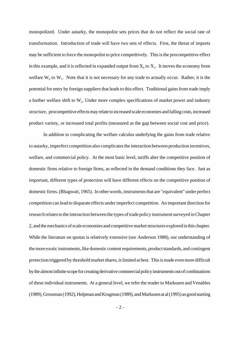
monopolized. Under autarky, the monopolist sets prices that do not reflect the social rate of

transformation. Introduction of trade will have two sets of effects. First, the threat of imports

may be sufficient to force the monopolist to price competitively. This is the procompetitive effect

in this example, and it is reflected in expanded output from X0 to X1. It moves the economy from

welfare W0 to W1. Note that it is not necessary for any trade to actually occur. Rather, it is the

potential for entry by foreign suppliers that leads to this effect. Traditional gains from trade imply

a further welfare shift to W2. Under more complex specifications of market power and industry

structure, procompetitive effects may relate to increased scale economies and falling costs, increased

product variety, or increased total profits (measured as the gap between social cost and price).

In addition to complicating the welfare calculus underlying the gains from trade relative

to autarky, imperfect competition also complicates the interaction between production incentives,

welfare, and commercial policy. At the most basic level, tariffs alter the competitive position of

domestic firms relative to foreign firms, as reflected in the demand conditions they face. Just as

important, different types of protection will have different effects on the competitive position of

domestic firms. (Bhagwati, 1965). In other words, instruments that are "equivalent" under perfect

competition can lead to disparate effects under imperfect competition. An important direction for

research relates to the interaction between the types of trade policy instrument surveyed in Chapter

2, and the mechanics of scale economies and competitive market structures explored in this chapter.

While the literature on quotas is relatively extensive (see Anderson 1988), our understanding of

the more exotic instruments, like domestic content requirements, product standards, and contingent

protection triggered by threshold market shares, is limited at best. This is made even more difficult

by the almost infinite scope for creating derivative commercial policy instruments out of combinations

of these individual instruments. At a general level, we refer the reader to Markusen and Venables

(1989), Grossman (1992), Helpman and Krugman (1989), and Markusen at al (1995) as good starting

- 3 -

points on abstract treatment of commercial policy under these conditions. For more concrete

examples involving applied studies of specific industries, see Baldwin and Krugman (1988a,b),

Dixit (1988), Feenstra (1988), and de Melo and Tarr (1992). On a regional basis, Cox and Harris

(1984) and Reinert, Shiells and Roland-Holst (1994) examine economic integration in North America,

while Venables and Smith (1986, 1988) examine economic integration in Europe. For multilateral

liberalization, recent studies include Haaland and Tollefson (1994) and Francois et al (1994, 1995).

To highlight how important the interactions between imperfect competition and choice of

commercial policy instruments can be, we close this section with a simple example involving tariffs

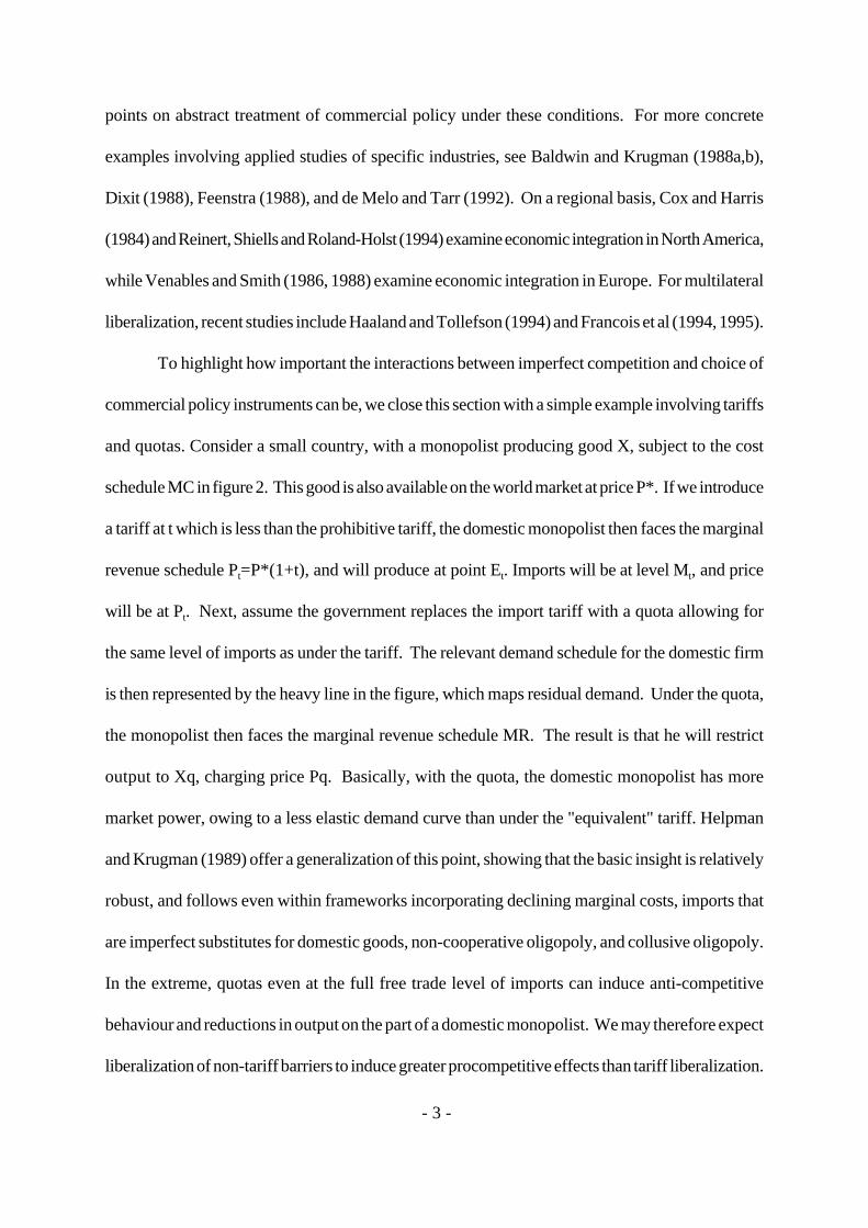
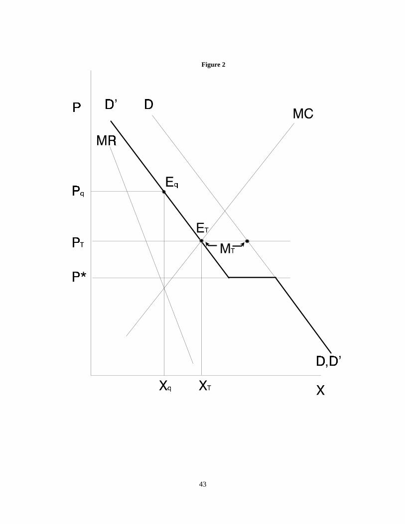
and quotas. Consider a small country, with a monopolist producing good X, subject to the cost

schedule MC in figure 2. This good is also available on the world market at price P*. If we introduce

a tariff at t which is less than the prohibitive tariff, the domestic monopolist then faces the marginal

revenue schedule Pt=P*(1+t), and will produce at point Et. Imports will be at level Mt, and price

will be at Pt. Next, assume the government replaces the import tariff with a quota allowing for

the same level of imports as under the tariff. The relevant demand schedule for the domestic firm

is then represented by the heavy line in the figure, which maps residual demand. Under the quota,

the monopolist then faces the marginal revenue schedule MR. The result is that he will restrict

output to Xq, charging price Pq. Basically, with the quota, the domestic monopolist has more

market power, owing to a less elastic demand curve than under the "equivalent" tariff. Helpman

and Krugman (1989) offer a generalization of this point, showing that the basic insight is relatively

robust, and follows even within frameworks incorporating declining marginal costs, imports that

are imperfect substitutes for domestic goods, non-cooperative oligopoly, and collusive oligopoly.

In the extreme, quotas even at the full free trade level of imports can induce anti-competitive

behaviour and reductions in output on the part of a domestic monopolist. We may therefore expect

liberalization of non-tariff barriers to induce greater procompetitive effects than tariff liberalization.

- 4 -

III. Firm-level costs

In empirical models, the cost structure of firms, and hence of industry, follows from the

choice of modelling technique and the observed data to which it is calibrated. One aspect which

has received intense scrutiny in recent years is returns to scale. Beginning with a study by Harris

(1984), a large literature on empirical modelling arose to evaluate trade liberalization under various

specifications of returns to scale.2 This new empirical research initiative was abetted by the intense

parallel interest among trade theorists in applying concepts from industrial organization to trade

theory.3 Both strains of work on firm-level scale economies confirm a basic conclusion of the earlier

literature on trade with industry-wide scale economies -- the results of empirical and theoretical

work grounded in classical trade theory can be contradicted, in magnitude and/or direction, when

scale economies or diseconomies play a significant role in the adjustment process.

Constant returns to scale (CRTS) is an attractive property in terms of flexibility and

parsimony. It facilitates practical data gathering, calibration, and interpretation of results. However,

its empirical veracity is open to question. In the real world, factors are heterogeneous in quality

and mobility, and changes in the level of output often involves changes in average cost, even for

relatively simple production processes. While there may be uncertainty about the precise magnitude,

scale economies are a fact of life and appear to be pervasive even in mature industries with diverse

firm populations. For these reasons, a re-appraisal of insights drawn from CRTS-based empirical

results is probably justified.

The most common departure from CRTS incorporates unrealized economies of scale in

production. Increasing returns to scale (IRTS) often takes the form of a monotonically decreasingly

average cost function, calibrated to some simple notion of a fixed cost intercept. In other words,

one assumes that marginal costs are governed by the preferred CRTS production function (usually

CES), but that some subset of inputs are committed a priori to production and their costs must

- 5 -

AC 'FCX

% MC (1)

AC ' X 2&1 f(T) where 0<2<1 (2)

be covered regardless of the output level. The total cost function may be homothetic (i.e. fixed

costs involve the same mix of inputs as marginal costs), or alternatively fixed costs may be assumed

to involve a different set of inputs. In either case, average costs are given by a reciprocal function

of the form

As an alternative, scale economies can also be specified as deriving from costs that enter

multiplicatively, with an average cost function like the following:

where f(T) represents the cost function for a homogenous bundle of primary and intermediate inputs.

This type of reduced form structure can be derived, for example, from scale economies due to returns

from specialization (i.e. an increased division of labour) inside firms. (Francois, 1990). In reduced

form, it can also represent returns to specialization on an industry-wide basis of intermediate inputs,

resulting in industry-wide scale effects. (Markusen 1990).

With scale economies as in equation (1) (i.e. with fixed costs), the CDR (cost disadvantage

ratio), as defined below, will vary with the scale of output. Alternatively, with a cost function like

(2), the CDR remains fixed. The properties of the two cost functions are illustrated in Figure 3.

Under either approach, one "only" needs to calibrate the cost function from engineering

estimates of the distance between average and marginal cost. With fixed costs, this also requires

some idea about how to impute fixed cost to initial factor and/or intermediate use. In practice,

it has become customary to appeal to the concept of a cost disadvantage ratio. This measure of

unrealized scale economies is generally defined as

- 6 -

CDR 'AC&MC

AC(3)

At the margin, output elasticities are equal to (1/(1-CDR)).

In practice, calibration of either (1) or (2) can be problematic. At a conceptual level,

estimated CDRs may be based on one level of "typical" production, while the benchmark dataset

we are working with corresponds to another. If we model scale economies with fixed costs and

variable CDRs (i.e. equation 1), then the CDR estimates can be inappropriate and even misleading.

At a more basic level, the pattern of citations in the empirical literature employing scale economies

is suspiciously circular. It converges on a set of engineering studies on scale elasticities, many of

which are surveyed by Pratten (1988), and many of which date from the 1950s, 1960s, and early

1970s. Given technical change over this period, including the introduction of numerically controlled

machinery, computerization of central offices, and the shift toward white collar workers and away

from production workers in the OECD countries these estimates appear somewhat stale. Clearly,

this is an important area for future research.

IV. Market power and homgeneous goods

A. perfect competition

The standard starting point for market structure in applied trade models, and our reference

point for the discussion in this section, is a competitive industry that can be described in terms of

a representative firm facing perfectly competitive factor markets and behaving competitively in

its relevant output markets. Under these assumptions, the representative firm takes price as given,

and the cost structure of the industry then determines output at a given price. Formally, we have:

- 7 -

P ' AC (4)

P ' MC (5)

P&MCP

'1, (6)

, ' &MQMP

PQ

(7)

Under increasing returns to scale at the firm level, equation (4) can be motivated by contestability,

with real or threatened entry forcing economic profits to zero. Demand for primary and intermediate

inputs will then depend on the specific cost structure that is assumed. If we assume constant instead

of increasing returns, average cost pricing then also implies pricing at marginal cost.

B. monopoly

Our first departure from the competitive paradigm is the case of monopoly. The monopoly

specification is a straightforward extension of perfect competition. In terms of equations (4) and

(5), we still have a representative firm in the sector under consideration. The difference lies in the

firm's pricing behaviour. In particular, the monopolist does not take price as given, but rather takes

advantage of her ability to manipulate price by limiting supply. This means that the pricing equation

(5) is then replaced by the following equation:

where the market elasticity of demand is given by

The relationship of price to average cost depends on our assumptions about the cost and

competitive structure of the industry. For example, with contestability and scale economies, entry

may still force economic profits to zero, such that the monopolist prices according to equations

- 8 -

B ' (P&AC)Q (8)

Si'dQdQi

(9)

(6) and (4). This is the approach taken in models with monopolistic competition. Alternatively,

we may instead have price determined by equation (6) in isolation from (4), such that demand

quantities at the monopoly price also then determine average cost. Equation (4) is then replaced

by a definition of economic profits.

C. homogeneous products and oligopoly

Between the perfect competition and monopoly paradigms lies a continuum of possible

firm distributions. When the number of firms is small enough for them to influence one another,

complex strategies can arise. We will not pretend to cover the full spectrum of oligopoly theory

in this chapter. Instead, we offer a set of representative specifications which indicate the decisive

role that firm interactions can play in determining price, quantity, efficiency and welfare.

One vehicle often used to explore oligopoly interactions is the so-called Cournot conjectural

variations model. Under this approach, we assume that each firm produces a homogeneous product,

faces downward sloping demand and adjusts output to maximize profits, with a common market

price as the equilibrating variable. We further assume, following Frisch (1933), that firms anticipate

or conjecture the output responses of their competitors. Consider an industry populated by n

identical firms producing collective output Q = nQi. When the ith firm changes its output, its

conjecture with respect to the change in industry output is represented by

- 9 -

Ai'PQi&TCi (10)

dAi

dQi

'P%QidPdQ

dQdQi

&dTCi

dQi

'P D&Qi

n,PQi

S&MC'0 (11)

P&MCP

'Sn, (12)

which equals a common value S under the assumption of identical firms. Combined with a

representative profit function

this yields the first-order condition,

and also the oligopoly pricing rule

The above expression encompasses a variety of relevant cases. The classic Cournot

specification corresponds to (S/n)=(1/n), where each firm believes that the others will not change

their output, and industry output changes coincide with its own. Price-cost margins vary inversely

with the number of firms and the market elasticity of demand, as logic would dictate. In the extreme

cases, a value of S=0 corresponds to perfectly competitive, average cost pricing, while S=n is

equivalent to a perfectly collusive or monopolistic market. The range of outcomes between these

extremes, as measured by 1 $ (S/n) $ 0 , can provide some insight into the significance of varying

degrees of market power.

D. market entry and exit

- 10 -

S'Sono

n(13)

In the previous section, we defined Cournot interactions with respect to a fixed number

of incumbent firms, implying barriers to entry (and exit). When we allow for the possibility of market

entry and exit, then the number of firms n becomes endogenous, and the competitive climate in

the industry under consideration varies accordingly.

Note that the price-cost margins in equation (12) vary with the number of firms. In particular,

margins shrink with an increase in the number of firms. This is the first effect of entry. In addition,

a major effect of entry and exit relates, under increasing returns, to firm level scale economies.

Entry and exit can alter the average scale of firm operations, other things equal, and in the increasing

and decreasing returns cases this can have aggregate efficiency effects.

The ultimate scope for entry, exit, or realization of scale economies in particular industries

is an empirical question. In the present context, entry and exit are basically model closure problems,

taking the form of limiting rules for incumbent profits, prices, or some other indicator of the return

on existing operations. In general, these rules should provide an explicit link between profits and

entry. We will briefly discuss two illustrative cases. One stylized approach involves assuming that

there is no actual entry or exit, but that the threat of entry forces incumbent firms to limit profits.

In this case, the scale of individual (representative) firm operations varies proportionately with

industry output, and changes in scale economies are easy to predict. An alternative is to allow

firm numbers to be endogenous and linked to profitability, while also specifying a secondary rule

linking incumbent pricing to the number of firms. It is then actual entry and exit that acts as an

explicit constraint on profitability. For example, endogenous Cournot conjectures of the form

- 11 -

imply that firms perceive their markets as becoming more competitive as the number of firms

increases.

E. dynamic interactions

While the conjectural variation approach to Cournot competition allows us to specify a

set of equilibria ranging from competition to monopoly, it has been criticized by a number of authors

as being an unrealistic and rather naive approach to dynamic market interactions.4 In recent years,

significant advances have been made in the theory of repeated games. It may be that, when

incorporated into applied models, these theoretical approaches yield more realistic approaches to

simulating market dynamics. The repeated game approach can be appealing not only because it

explicitly considers the sequential and historical aspects of competition, but also because it opens

up a richer universe of strategic opportunities and solution concepts. At the same time, depending

on the context of the modelling exercise, one must be careful not to hang too much significance

on the benefits of such methods. It is not always clear what is gained when complex, firm level

interactions are explicitly modelled for a heterogeneous sector such as "other machinery" or

"transport equipment" that is clearly a collection of firms and industries (such as bicycles,

automobiles, and airplanes) that are only related directly through statistical aggregation. Even at

the level of only a few firms (like automobiles or mid-sized aircraft), lack of data may mean that

we have replaced conjectural variations with conjectural data manufacturing.

Repeated games can yield tacit collusion. (Tirole 1988; Shapiro 1989). The simple Cournot

strategy, for example, emerges as the Nash equilibrium for a repeated game. However, this strategy

does not maximize profits for the industry as a whole or for individual firms. The same is true of

Bertrand competition. Under both price and quantity competition, we can construct repeated games

that yield sustained collusion with higher profits. Use of repeated game frameworks may therefore

- 12 -

qj,r ' jR

i'1"j, i,r X

Dj

j, i, r

1/Dj

(14)

allow for modelling of cases where trade liberalization, through its effect on relevant variables,

can induce changes in the incentives for collusion (with reversion from collusion to Cournot

equilibria, for example).

V. Heterogeneous goods

We turn next to market power in models that explicitly incorporate heterogeneous goods,

emphasizing specifications involving two or more regions. In the first case, a class of heterogeneous

goods is assumed to be differentiated by country of origin. This is the Armington assumption.

The second specification is based on firm-level product differentiation.

A. Market power in Armington models

In Armington models, goods are differentiated by country of origin, and the similarity of goods

from different regions is measured by the elasticity of substitution. Formally, within a particular

region, we assume that demand goods from different regions are aggregated into a composite good

according to the following CES function:

In equation (14), Xj,i,R is the quantity of Xj from region i consumed in region r. The elasticity of

substitution between varieties from different regions is then equal to Fj , where Fj = 1/(1-Dj). For

tractability, we focus here on the non-nested case, where Fj is identical across regions, and is equal

to the degree of substitution between imports, as a class of goods, and domestic goods.5 Within

a region, the price index for the composite good q j,r can be derived from equation (14):

- 13 -

Pj,r ' jR

i'1"i ,r

Fj Pi,r1&Fj

1&1/Dj

(15)

Xj, i, r ' ["j, i,r /Pj, i, r]Fj [ j

R

i'1"j, i,r

Fj Pj, i,r1&Fj ]&1 Ej, r

' ["j, i,r /Pj, i,r]Fj Pj, r

Fj&1 Ej,r

(16)

,j,i,r ' Fj % (1&Fj) jR

k'1

"j,k,r

"j,i, r

Fj Pj, kr

Pj, i,r

1&Fj&1

(17)

At the same time, from the first order conditions, the demand for good Xj,i,r can then be shown

to equal

where E j represents economywide expenditures in region r on the sector j Armington composite.

From equation (16), the elasticity of demand for a given variety of good Xj, produced in region

i and sold in region r, will then equal:

The last term measures market share.

monopoly

At this stage, there are a number of ways to introduce imperfectly competitive behaviour.

For example, for a monopolists in each region that can price discriminate between regional markets,

the regional elasticity of demand (and hence the relevant mark-up of price over marginal cost) is

determined in each market by equation (17). This implies, potentially, n×R2 sets of elasticity and

price mark-up equations for an R region, n sector model. In models where different sources of

- 14 -

,j,i ' F % (1&F) .j, i (18)

. j, i ' jR

r'1

Xj, i,r

Xj, ijR

k'1

"j, k,r

"j,i,r

Fj Pj, kr

Pj, i,r

1&Fj&1

(19)

demand can potentially source imported inputs in different proportions (like the SALTER and GTAP

models), we then have a potential for (n+k)×n×R2 elasticity and mark-up equations, where k is

the number of final demand sources in each region. Hence, in large multiregion models, full regional

price discrimination for each product in each region can add a great deal of numerical complexity

to the model.

A greatly simplifying assumption involves assuming a monopolist that does not price

discriminate, but instead charges a single mark-up. From equation (17), the aggregate elasticity

of demand will then be determined by a combination of Fj and a weighting of (1-Fj) determined

by regional market shares. One option is to assume that each firm forms a conjecture about the

value of this weighting parameter, represented by ..6 If each firm assumes that .j,i is fixed, this

means it forms a conjecture about the elasticity of demand based on .j,i and Fj. For a monopolist

in region i producing j, we then have:

Instead of assuming that . is fixed (at least for relevant equilibria), we can also specify an explicit

definition based on equation (17). For each sector, we must then add the equations necessary to

endogenize ..

There are trade-offs between the complexity of the model, and the degree of discriminatory

power allowed for monopolists. If we expect significant pro-competitive effects related to changes

in perceived market power in particular markets, through changes in either ,j,i or .j,i , then we should

- 15 -

P&MCP

'Sn,

'Sn

F% (1&F).&1(20)

explicitly specify relative market power in those markets that are at least partially segmented through

tariffs, transport costs, or other trade barriers.

oligopoly

If we start with the non-discriminatory case of market power, then extending our model from

monopoly to oligopoly is relatively straightforward. We keep the simplifying assumption, introduced

earlier, that under oligopoly firms are identical. The key difference is that they now produce a

regionally homogeneous product. Demand for a regional product is downward sloping, as defined

by equation (17). We further assume that firms adjust output to maximize profits, with a common

market price as the equilibrating variable, and that firms anticipate or conjecture the output responses

of their competitors. This leaves us with a variation of the basic oligopoly pricing rule

B. Firm-level product differentiation

Next, we turn to firm-level product differentiation. This approach builds on the theoretical

foundations laid by Ethier (1979, 1982), Helpman (1981), and Krugman (1979, 1980). Arguments

for following this approach, where differentiation occurs at the firm level, have been offered by

Norman (1990) and Brown (1987). The numeric properties of this type of model have been explored

in a highly stylized model by Brown (1994). Theoretical properties of the type of model developed

here, which explicitly allows for firms having different market shares in the various markets in which

they operate, have been examined by Venables (1987).

- 16 -

qj,r ' jn

i'1"j, i,r X

D j

j, i, r

1/Dj

(21)

general specification of monopolistic competition

Formally, within a region r, we assume that demand for differentiated intermediate products belonging

to sector j can be derived from the following CES function, which is now indexed over firms or

varieties instead of over regions. We have

where "j,i,r is the demand share preference parameter, Xj,i,r is demand for variety i of product j in

region r, and Fj = 1/(1-Dj) is the elasticity of substitution between any two varieties of the good.

Note that we can interpret q as the output of a constant returns assembly process, where the resulting

composite product enters consumption and/or production.7 Equation (21) could therefore be

interpreted as representing an assembly function embedded in the production technology of firms

that use intermediates in production of final goods, and alternatively as representing a CES

aggregator implicit in consumer utility functions. In the literature, both cases are specified with

the same functional form. Because most industrial trade involves intermediates, we lean towards

the former interpretation. While we have technically dropped the Armington assumption by allowing

firms to differentiate products, the vector of " parameters still provides a partial geographic anchor

for production.8

In each region, industry j is assumed to be monopolistically competitive. This means that

individual firms produce unique varieties of good j, and hence are monopolists within their chosen

market niche. Given the demand for variety, reflected in equation (21), the demand for each variety

is less than perfectly elastic. However, while firms are thus able to price as monopolists, free entry

drives their economic profits to zero, so that pricing is at average cost. The joint assumptions of

- 17 -

Pf, i&MCf, i

Pf, i

'1,f, i

(22)

Pf, i ' ACf, i (23)

,j, f, i ' Fj % (1&Fj) .j, f, i (24)

. j, f i' j

R

r'1

Xj, fi ,r

Xj, f i

jn

k'1

"j, k, r

"j, fi ,r

Fj Pj,k, r

Pj, f, r

1&Fj

&1

(25)

Zj, i ' jni

f'1TCj, i, f (26)

average cost pricing and monopoly pricing imply the following conditions for each firm fi in region

i:

The elasticity of demand for each firm fi will be defined by the following conditions.

In a fully symmetric equilibrium, .=n-1. Under more general conditions, it is a quantity weighted

measure of market share. To close the system for regional production, we index total resource

costs for sector j in region i by the resource index Z. Full employment of resources hired by firms

in the sector j in region i then implies the following condition.

- 18 -

qj,r ' [ jR

i'1

nj,i"j,i,r x̄j,i,rDj ]

1Dj (27)

In models with regionally symmetric firms (so that Z j,i = n j,i × TC j,i ), equations (22) - (26), together

with the definition of AC=AC(x), define a subsystem that determines six sets of variables: x, ,,

., P, n, and the cost disadvantage ratio CDR= (1- MC/AC).

These equilibrium conditions are represented graphically in Figure 4. The full employment

of resources at level Z in the regional sector implies, from equation (26), possible combinations

of n and x mapped as the curve FF. At the same time, demand for variety, combined with zero

profit pricing (equations (22) and (23)), imply demand-side preference for scale and variety mapped

as the curve ZZ. Equilibrium is at point E0. Holding the rest of the system constant, expansion

of the sector means the FF curve shifts out, yielding a new combination of scale and variety and

point E1. The exact pattern of shifts in n and x depends on the assumptions we make about the

cost structure of firms, and about the competitive conditions of the sector. It may also be affected

by general equilibrium effects.

some simplifications: variety scaling

To simplify the system of equations somewhat, symmetry can be imposed on the cost structure

of firms within a region. Regional symmetry means that, in equilibrium, regional firms will produce

the same quantity of output and charge the same price. Under variety scaling, we further assume

that the CES weights applied to goods produced by sector j firms from region i, when consumed

in a particular region r, are equal. This means we can rewrite equation (8) as follows.

Where x& is the identical consumption in region r of each variety produced in region i. Upon

inspection of equations (27) and (14), it should be evident that the Armington assumption and firm

- 19 -

qj,r ' [ jR

i'1

(j, i,r-xj, i,r

Dj]

1Dj

(j, i,r ' "j, i,r nj, i 01&Dj

-xj,i,r

'nj, i

nj, i 0

(1&Dj)/Dj

Xj, i,r

(28)

level product differentiation, in practice, bear a number of similarities. The primary difference is

that, in equation (27), the CES weights are now endogenous, as they include both variety scaling

effects and the base CES weights. We can make a further modification to equation (27). Noting

that total quantities are Xj,i,r=nj,r×x& , we then have:

where x̃j,i is variety-scale output, and where nj,i 0 is the benchmark number of firms. Note that x̃j,i

= Xj,i in the benchmark.

When we specify the system of equations for monopolistic competition using a variation

of equation (22), the final set of equations for producing sector j composite commodities is then

almost identical to that employed in standard, non-nested Armington models. The key difference

is that the relevant CES weights are endogenized through x̃j,i, as defined by equation (28). In fully

symmetric equilibria, the reader should be able to verify that complete firm exit from particular

regions is possible, since the regional CES weights are simply equal to the number of firms, which

collapse to zero with full exit. Depending on the specification of the structure of monopolistically

competitive markets, as detailed below, the combination of output and variety scaling can then

specified as part of the regional production function for x̃j,i.

scale economies from fixed costs

- 20 -

C(xj, i) ' ("j, i % $j, i xj, i) PZj, i (29)

AC&MCAC

'"j, i

"j, i%$j, i xj, i

'1,j, i

(30)

,j,i ' Fj % (1&Fj) .j,i (31)

. j,i ' jR

r'1

-xj,i,r

-xj,i

jR

k'1nj,k

"j, k,r

"j, i, r

Fj Pj,k, r

Pj, i,r

1&Fj&1

(32)

We will focus on two particular specifications of increasing returns. The first is a variation of

equation (1), in which we assume that the cost function, while exhibiting increasing returns due

to fixed costs, is still homothetic. In particular, for a firm in region i, we have:

where "r,i and $r,i represent fixed and marginal costs, and PZj,i represents the price for a bundle of

primary and intermediate inputs Zj,i, where the production technology for Zj,i is assumed to exhibit

constant returns to scale.

Substituting equation (29) into (22), (23), and (26), the system of equations (22) through

(26), along with the definition of average cost, can be used to define general conditions for

equilibrium in a monopolistically competitive industry. Starting from equations (22) and (23), the

elasticity of demand can be related directly to the cost disadvantage ratio.

The remainder of the system is as follows:

- 21 -

Zj,i ' nj,i ("j,i%$j,i xj,i) (33)

-Xj,i

'Zj,i 1

Zj,i 0

(1&Dj)/Dj

Xj, i (34)

Given the resources allocated to sector j in region i, as measured by the index Zj,i, equations (30)

through (33) define a subsystem of 4 equations and 4 unknowns: nj,i , xj,i , .j,i , and ,j,i. In addition,

the value of x̃j,i is then determined by equation (28), while producer price is set at average cost.

Note that the price terms in equation (32) are internal prices, and will hence reflect trade barriers

and other policy and trade cost aspects of the general equilibrium system, implying still more

equations linking producer and consumer prices.

A special case of this specification involves "large group" monopolistic competition. In

large group specifications, we assume that n is arbitrarily large, such that .j,i is effectively zero,

and hence, through equations (30) and (31), the elasticity of demand and the scale of individual

firms are also fixed. In this case, changes in the size of an industry involve entry and exit of

identically sized firms. The full set of equations then collapses to the following single equation:

Here, Xj,i is produced subject to constant returns to scale, given entry and exit of identical firms

of fixed size, which follows from our assumptions about the cost function for Zj,i. At the same

time, changes in variety are directly proportional to changes in Zj,i.

It can be shown that proportional changes in x̃j,i relate to proportional changes in Zj,i:

- 22 -

¸-Xj,i

' (Fj /(Fj&1))¸

Zj, i%

(Fj&,j, i).j,i

(Fj&1)(1&.j, i)CDR

¸.j,i

(35)

What does equation (35) tell us? The first term is clearly positive, and relates to the impact of

increased resources on the general activity level of the sector, given its structure. The second term

relates to changes in the condition of competition. Controlling for changes in market share for

the entire regional industry, changes in .j,i are proportional to changes in the inverse number of

firms in the industry. Hence, we expect the last term to have a negative sign, but also to become

smaller as the sector expands. In particular, as the sector expands, the value (F-,) converges on

zero, as does .j,i ,so that this last term becomes less important. This follows from the procompetitive

effects of sector expansion. As the sector expands, new entrants intensify the conditions of

competition, forcing existing firms down their cost curves and hence squeezing the markup of price

over marginal cost. As the sector becomes increasingly competitive, the marginal benefits of devoting

more resources to the sector are greater, until at the limit the output elasticity for variety-scaled

output converges on (1/D). This is the large group case, where (F=,), such that the second term

vanishes.

scale economies with fixed scale effects

We close this section with an alternative specification of monopolistic competition, in which cost

functions for individual firms take the form of equation (2):

- 23 -

C(xj, i) ' xj, i2j, i PZj, i

where 0<2j, i<1(36)

Zj, i ' nj, i xj, i2j, i (39)

(1&2j,i)&1 ' Fj % (1&Fj) .̄j,i (37)

.̄ j,i ' jR

r'1

-Xj,i,r

-Xj,i

jR

k'1nk

"j, k,r

"j, i, r

Fj Pj,k, r

Pj, i,r

1&Fj&1

(38)

¸-Xj, i

' (Fj /(Fj&1))¸

Zj,i&

(Fj&,j, i)

(Fj&1)(,j,i& 1)

¸nj, i

(40)

With costs described by equation (36), the cost disadvantage ratio is constant. From equations

(22) through (25), this requires entry and exit such that the parameter .j,i remains constant. This

ensures that monopoly pricing is consistent with zero profits. Hence, the relevant subsystem of

equations will be the following, along with equation (28):

In purely symmetric equilibria, where firms are identical across regions, this specification

yields a fixed number of firms, with sector expansion characterized strictly by expansion of existing

firms. In this case, we have .=(1/n). Given estimated cost disadvantage ratios, equation (37) can

therefore be used to calibrate the value of F.

We can again show that changes in x̃j,i relate to proportional changes in Zj,i :

- 24 -

Equation (40) is quite similar to equation (35). The difference is that the second term, which is

again negative, now relates to the entry of additional firms. In a framework that now emphasizes

output scaling, entry reduces the cost benefits of increased scale somewhat (the first term), though

this is moderated by the varietal benefits of entry. In symmetric equilibria or under the large group

assumption, the second term is zero.

In the large group case, equations (35) and (40) are identical. Hence, while the large group

specification, with fixed costs, yields pure variety scaling, the fixed CDR specification yields output

scaling. These two mechanisms both imply the samel reduced functional form. In both cases, the

output elasticity of variety-scale output is 1/(1-CDR). In terms of figure 4, these two cases

correspond to curves Z1Z1and Z2Z2.

VI. An application to Korea

We now turn to a specific application involving scale economies and imperfect competition. The

basic model we work with is a Korea-focused multi-region general equilibrium. We will limit

ourselves to a Uruguay Round scenario, involving multilateral liberalization. While the model is

basically the same as standard CRTS Armington models, some important features should be

highlighted. First, the current account balance is held constant in all simulations. In addition, the

Armington structure is a non-nested structure. Finally, as described below, the assumption of

constant returns to scale (CRTS) and perfect competition is replaced by various specifications of

increasing returns to scale (IRTS) and imperfect competition.

Table 1 presents the trade and scale elasticities employed in the numeric assessments. The

CDR estimates are taken from various sources (primarily Pratten 1988). When specifying oligopolistic

competition, we limit ourselves to the Korean manufacturing sector. In this case, we work with

Cournot conjectural variations, as defined earlier in the paper, assuming two values for (S/n), (S/n)

- 25 -

Pj, i ' ACj, i 1&CDRj, i 1& (Sj, i /(nj, i,j, i))&1 (41)

= 0.2 and 0.5. These values are consistent with classic Cournot competition with 5 firms and 2

firms, respectively. In general, with Cournot competition and identical firms, the markup of price

over average cost is be defined as follows:

Upon inspection of equation (41), it should be clear that, with scale economies, Cournot behaviour

can be inconsistent with positive profits. In particular, with a large enough CDR or highly elastic

demand, pricing such that MR=MC will imply setting P<AC.

Table 2 presents estimated oligopoly markups for Korean industry, based on equation (41),

and derived from the benchmark 1992 dataset. These markups are a function of market shares,

and of the substitution elasticities presented in Table 1. In some cases, like processed food, home

market shares, and hence the implicit markups, are a direct result of import protection. This becomes

evident when we examine the output effects of trade liberalization, which exhibit significant

procompetitive features for these same sectors.

Table 3 presents estimated output effects in Korea under alternative assumptions about

Korean industry. The first set of simulation results involves CRTS and perfect competition, and

serves as a reference experiment. The next two columns in the table correspond to IRTS and average

cost pricing. The second column involves scale economies with fixed costs, while the third involves

scale economies and fixed CDRs. The estimated effects are almost identical, implying that the choice

of specification of scale economies is not very important in the present experiment. Note that for

a number of industrial sectors, output effects are almost double their values under CRTS. This

is one of our first indications of the potential importance of scale effects when evaluating trade

liberalization.

- 26 -

We next turn to Cournot behaviour, as reported in columns 4,5, and 6 of Table 3. The

first two of these sets of results involve CRTS. Evidence of the procompetitive effects of trade

liberalization can be seen if we compare these results with those in the first column. Recall from

Table 2 that some sectors, like processed food and chemicals, had particularly high estimates of

markups of price over average cost. Because trade liberalization erodes the market power derived

from protection, these markups are reduced and output increased in Cournot sectors. The result

in some sectors, like chemicals and processed foods, is output effects roughly twice as great as

those estimated under CRTS and perfect competition. Finally, the last column of the table combines

Cournot behaviour with increasing returns. The result, across a broad range of sectors, is

substantially greater output effects than those reported in the other columns. This follows from

the effects of reduced market power, combined with the output boost that follows from falling

average costs. Taken together, the result of IRTS and Cournot is that several manufacturing sectors

expand by roughly twice the amount estimated in the benchmark experiment.

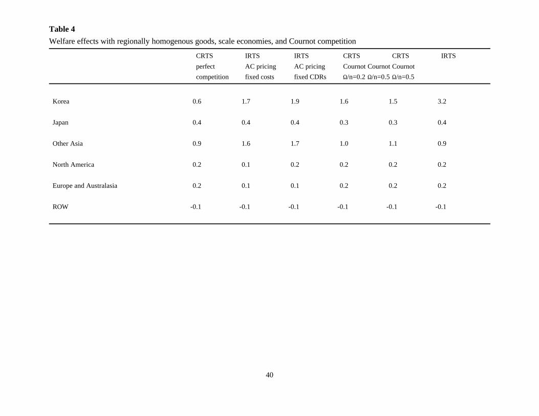
The welfare effects reported in Table 4 correspond to the same specifications employed

in Table 3. Recall that we only introduce Cournot behaviour in Korea, so that, not surprisingly,

the greatest variation in welfare results relates to Korea. In particular, the introduction of Cournot

behaviour in isolation from scale economies, or IRTS in isolation from imperfectly competitive

behaviour, implies a significant magnification of the estimated welfare gains for Korea. In particular,

while our benchmark case involves a 0.6 percent increase in welfare, this is basically increased by

a factor of 3 in columns 2 through 5. Column 6 presents estimates where we have introduced both

scale economies and Cournot behaviour. Here, welfare increases by 3.2 percent, as compared to

0.6 percent in the benchmark and 1.5 to 1.9 percent in columns 2 through 5.

Finally, Table 5 contrasts the implications of scale economies under national product

differentiation (the Armington assumption), with scale economies under firm level product

- 27 -

differentiation (large group monopolistic competition.) While the result is a magnification of

estimated benefits for Korea (4.6 percent vs. 1.9 percent in columns 3 and 2), this is not true for

all regions. For the region "Other Asia", welfare gains are greater with national product

differentiation. For all other regions excluding ROW, firm level product differentiation clearly implies

greater pro-competitive benefits then those estimated under Armington preferences.

VII. Summary and Closing Ruminations

This paper has been concerned with relationships between trade policy, imperfect competition,

and industry performance. Our basic goal has been to provide an overview of linkages between

trade policy and competitive behaviour, including the presentation of a menu of relatively standard

specifications of imperfect competition and scale economies. As the now extensive body of applied

research demonstrates, these linkages can easily dominate, in sign and/or magnitude the production

and welfare effects estimated under the perfect competition paradigm.

The empirical literature confirms a basic finding of the new trade theories, suggesting that

there may be small potential gains from mild unilateral protection. However, these numerically

estimated gains, like their theoretical counterparts, are often the product of single market or partial

equilibrium modeling exercises. Dixit and Grossman (1984) have rightly objected to drawing policy

conclusion from this type of single-market framework for a simple reason. In general equilibrium,

it is impossible to subsidize or effectively protect the entire economy. Targeting expansion of some

increasing returns sectors implies targeting contraction of other ones. In addition, as Helpman

and Krugman (1989, Chapter 8) have noted, while there may be small gains from unilateral

protection, the apparent costs of mutual protection are magnified when scale economies and imperfect

competition enter the picture. A corollary of this last point is that bilateral and multilateral trade

liberalization tend to imply much greater welfare gains, once we allow for imperfect competition

- 28 -

and scale economies, than analyses based on perfect competition and constant returns to scale would

otherwise imply.9

As an illustration, we have offered a set of Korea-focused Uruguay Round simulation results.

These results highlight rather starkly the significant role that imperfect competition can play in

assessments of trade liberalization. Not surprisingly, our estimates prove sensitive to the assumptions

we make. However, taken as a whole, the pattern of results demonstrate that the procompetitive

effects of trade liberalization, including falling market power and expanded output in imperfectly

competitive sectors, may be some of the most substantial effects following from trade liberalization,

particularly for developing countries. At a minimum, it is clear that the constant returns, perfect

competition paradigm suppresses a number of potentially powerful mechanisms linking trade policy

with industry performance.

- 29 -

1. See Roberts and Tybout (1990) and Devarajan and Rodrik (1989ab), Rodrik (1988), and de

Melo (1988) for more on the perspective from development studies.

2. See de Melo and Tarr (1992) for methodological discussion, Reinert, Roland-Holst, and Shiells

(1994) and Francois et al (1995) for more recent applications.

3. See e.g. Krugman (1985) for examples from this literature.

4. See e.g. Shapiro (1989).

5. A variation on this approach involves nesting the Armington structure, so that imports from

different sources are first aggregated, and the composite good then competes with domestic goods

in a second Armington aggregation function. In the present context, this would involve another

set of equations for each region, though the discussion would be qualitatively similar.

6. Clearly, this raises the question of how to calibrate ., and the relative advantages and disadvantages

of endogenizing >. In the numeric examples in this paper, we could have employed estimates of

the reduced form elasticity of demand in general equilibrium, based on perturbations of price, to

calibrate ,j,R, based on the assumption that firms correctly know the marginal elasticity of demand,

and assuming that this value is constant in counterfactual simulations. We have chosen instead

to simplify the demand structure slightly, and to directly calculate these share parameters.

7. An approach sometimes followed involves monopolistic competition within regions, with trade

only involving composite goods. Trade then is not based on firm level differentiation (i.e.

monopolistic competition). Rather, trade is then based on the Armington assumption regarding

regional composite goods. The basic difference between this approach and the one developed in

the text is the relaxation of the linkage between upper-tier substitution elasticities and measures

of market power for regional firms. We leave it to the reader to verify, from equations (35) and

(40), that this implies a model exhibiting, in reduced form, external scale economies at the regional

Endnotes

- 30 -

level.

8. The Armington assumption, or more generally allowing for region-specific differentiation, ensures

uniqueness of production equilibria with v factors and n>v goods. Otherwise, we would need to

adopt a specific-factor specification, or in some other way ensure the number of goods did not

exceed the number of factors in order to solve for unique production and trade patterns for a given

set of prices. With inter-sectoral mobility of capital and labour, and more than two goods, if we

assumed differentiation was only at the firm level, and that all firm output entered the CES aggregator

identically regardless of origin (i.e. with identical weights), free trade production patterns with two-

way trade, at least in an integrated equilibrium, would be indeterminate. See Dixit and Norman

(1980, "Problems of generalization," in Theory of International Trade, pp. 56-59). In general, the

introduction of scale economies raises the likelihood of multiple equilibria.

9. To quote Venables and Smith, "It seems unlikely, to say the least, that in a world in which all

countries pursue restrictive trade policies the potential benefits of scale economies will actually

be realized. One of the reason we have institutions such as the GATT is to discourgae this type

of beggar-thy-neighbour policies. The fact that our analysis indicates that there may be significant

potential gains from policy intervention should not be taken as establishing a case for nationalistic

trade restrictions but as providing a strong rationale for negotiated reductions in trade barriers."

(Venables and Smith, 1988, p 660).

- 31 -

References

Anderson, J.E. (1988), The Relative Inefficiency of Quotas, MIT Press: Cambridge.

Baldwin, R.E. and P. Krugman. "Industrial Policy and International Competition in Wide-Bodied

Jet Aircraft." In R.E. Baldwin, ed., Trade Policy Issues and Empirical Analysis. Chicago:

U. of Chicago Press, 1988.

Baldwin, R.E. and P. Krugman. "Market Access and International Competition: A Simulation

Study of 16K Random Access Memories." In R.C. Feenstra, ed., Empirical Methods for

International Trade. Cambridge: MIT Press, 1988.

Bhagwati, J.N. (1965), "On the Equivalence of Tariffs and Quotas," in R.E. Baldwin et al, eds.,

Trade, Growth, and the Balance of Payments: Essays in Honor of Gottfried Haberler,

Chicago: Rand McNally.

Brander, J.A., and B.J. Spencer (1984), “Tariff Protection and Imperfect Competition,” in H.

Kierkowski (ed.), Monopolistic Competition and International Trade, Oxford: Oxford

University Press.

Brown, D.K. (1994), "Properties of Applied General Equilibrium Trade Models with Monopolistic

Competition and Foreign Direct Investment," in J.F. Francois and C.R. Shiells (eds.),

Modelling Trade Policy: AGE Models of North American Free Trade, Cambridge

University Press.

Brown, D.K. (1987), "Tariffs, the Terms of Trade and National Product Differentiation,"

Journal of Policy Modelling, 9, 503-526.

Cox, D. and Harris, R. 1985. "Trade Liberalization and Industrial Organization: Some Estimates

for Canada," Journal of Political Economy vol 93, 115-145.

- 32 -

Dervis, K., J. de Melo, and S. Robinson (1982), General Equilibrium Models for Development

Policy, Cambridge: Cambridge University Press.

Devarajan, S., and D. Rodrik (1988a), "Trade Liberalization in Developing Countries: Do Imperfect

Competition and Scale Economies Matter?" American Economic Review, Papers and

Proceedings, 283-287.

Devarajan, S., and D. Rodrik (1988b), "Pro-competitive Effects of Trade Reform: Results from

a CGE Model of Cameroon," Working Paper, Harvard University.

Dixit, A. "Optimal Trade Policy and Industrial Policies for the U.S. Automobile Industry," in R.C.

Feenstra, ed., Empirical Methods for International Trade, MIT Press: Cambridge, 1988.

Dixit, A. and G. Grossman (1984), "International Trade Policy with Several Oligopolistic

Industries," discussion paper in economics no. 71, Woodrow Wilson School, Princeton

University.

Eastman, H. and S. Stykolt (1960), "A Model for the Study of Protected Oligopolies," Economic

Journal, Vol. 70, pp. 336-47.

Eaton, J, and G.M. Grossman (1986), "Optimal Trade and Industrial Policy Under Oligopoly,"

Quarterly Journal of Economics, 101, pp.383-406.

Ericson, R., and A. Pakes (1989), "An Alternative Theory of Firm and Industry Dynamics,"

Discussion Paper No. 445, Columbia University.

Ethier, W. (1982), “National and International Returns to Scale in the Modern Theory of

International Trade,” American Economic Review, 72 (June), 950-959.

Feenstra, R.C. "Gains from Trade in Differentiated Products: Japanese Compact Trucks," in R.C.

Feenstra, ed., Empirical Methods for International Trade, MIT Press: Cambridge, 1988.

- 33 -

Francois, J.F., B. MacDonald, H. Nordström (1995), “Assessing the Uruguay Round,” in W. Martin

and A. Winters, eds. The Uruguay Round and the Developing Economies, The World Bank

discussion paper 201.

Francois, J.F., B. MacDonald, H. Nordström (1995), “The Uruguay Round: A Global General

Equilibrium Assessment,” CEPR discussion paper, November 1994.

Francois, J.F. and Shiells, C.R. (1994) Modelling Trade Policy: AGE Models of North American

Free Trade, Cambridge University Press.

Francois, J.F. (1992), “Optimal Commercial Policy with International Returns to Scale,” Canadian

Journal of Economics, 23, 109-124.

Freidman, D. (1971), “A Non-Cooperative Equilibrium for Supergames,” Review of Economic

Studies, 38, 1-12.

Fudenberg, D., and J. Tirole (1986), “Dynamic Models of Oligopoly,” in A. Jacquemin (ed.),

Fundamentals of Pure and Applied Economics, vol. 3, New York: Harwood.

Grossman, G.M. (1991). Imperfect Competition and International Trade, MIT Press: London.

Haaland, J. and T.C. Tollefsen (1994), "The Uruguay Round and Trade in Manufactures and

Services. General Equilibrium Simulations of Production, Trade and welfare Effects of

Liberalization," CEPR discussion paper 1008.

Harris, R. (1984), "Applied General Equilibrium Analysis of Small Open Economies with Scale

Economies and Imperfect Competition," American Economic Review, 74, 1016-1033.

Helpman, E. and P. Krugman (1985), Market Structure and Foreign Trade, MIT Press,

Cambridge.

- 34 -

Helpman, E. and P. Krugman (1989), Trade Policy and Market Structure, MIT Press,

Cambridge.

Krugman, P.R. (1980), “Scale Economies, Product Differentiation, and the Pattern of Trade,”

American Economic Review, 70 (December), 950-959.

Krugman, P.R. (1979), “Increasing Returns, Monopolistic Competition, and International Trade,”

Journal of International Economics, 9, 469-479.

Markusen, J.R., J.R. Melvin, W.H. Kaempfer, and K.E. Maskus, (1995), International Trade:

Theory and Evidence, McGraw-Hill: London.

Markusen, J.R. and A.J. Venables (1988), "Trade Policy with Increasing Returns and Imperfect

Competition: Contradictory Results from Competing Assumptions," Journal of International

Economics 24(May): 299-316.

Markusen, J.R. (1990), “Micro-Foundations of External Scale Economies,” Canadian Journal

of Economics, 23, 285-508.

Melo, J. de, and D.W. Roland-Holst (1991), "An Evaluation of Neutral Trade Policy Incentives

Under Increasing Returns to Scale," with J. de Melo, in J. de Melo and A. Sapir (eds.),

Essays in Honor of Béla Balassa, London: Basil Blackwell.

Melo, J. de, and D. Tarr (1992), A General Equilibrium Analysis of US Foreign Trade Policy,

MIT Press.

Norman, V.D. (1990), "Assessing Trade and Welfare Effects of Trade Liberalization: A

Comparison of Alternative Approaches to CGE Modelling with Imperfect Competition,"

European Economic Review 34: 725-745.

Osborne, M., and A. Rubinstein (1990), Bargaining and Markets, San Diego: Academic Press.

- 35 -

Pakes, A.(1993), "Dynamic Structural Models: Problems and Prospects. Part II: Mixed Continuous

Discrete Models and Market Interactions," in J.J. Laffont and C. Sims (eds.), Advances

in Econometrics, Proceedings of the Sixth World Congress of the Econometric Society,

Barcelona.

Pakes, A., and P. McGuire (1992), "Computing Markov Perfect Nash Equilibria: Numerical

Implications of a Dynamic Differentiated Product Model," Working Paper No. 119, National

Bureau of Economic Research, Cambridge, January.

Pakes, A., and G.S. Olley (1992), "The Dynamics of Productivity in the Telecommunications

Equipment Industry," Working Paper No. 3977, National Bureau of Economic Research,

Cambridge, January.

Pratten, C. (1988), "A Survey of the Economies of Scale," in Research on the Cost of Non-Europe,

vol 2, Brussels: Commission of the European Communities.

Roberts, M.J., and J.R. Tybout (1990), "Size Rationalization and Trade Exposure in Developing

Countries," Working Paper, Department of Economics, Georgetown University, May.

Rodrik, D. (1988), "Imperfect Competition, Scale Economies and Trade Policy in Developing

Countries," in R. Baldwin (ed.), Trade Policy Issues and Empirical Analysis, University

of Chicago Press and N.B.E.R.

Roland-Holst, D.W., Reinert, K.A., and C.R. Shiells (1994), "A General Equilibrium Analysis

of North American Integration," in J.F. Francois and C.R. Shiells (eds.), Modelling Trade

Policy: AGE Models of North American Free Trade, Cambridge University Press.

Roland-Holst, D.W., and D. van der Mensbrugghe (1995), “Empirical Implementation of the CDE

Production Technology,” Working Paper, OECD Development Centre, Paris.

- 36 -

Rotemberg, J., and G. Saloner (1986), “A Supergame-Theoretic Model of Business Cycles and

Price Wars During Booms,” American Economic Review, 76, 390-407.

Shapiro, C. (1989), “Theories of Oligopoly Behaviour,” in R. Schmalansee and R. Willig (eds.)

Handbook of Industrial Organization, Amsterdam: North Holland.

Smith, A., and A.J. Venables (1988), "Completing the Internal Market in the European Community,"

European Economic Review, 32, 1501-1525.

Tybout, J.R. (1989), "Entry, Exit, Competition and Productivity in the Chilean Industrial Sector,"

Working Paper, Trade Policy Division, The World Bank, May.

Tybout, J.R., V. Corbo, and J. de Melo (1988), "The Effects of Trade Reform on Scale and

Technical Efficiency,"

Venables, A. and Smith, A. (1986), "Trade and Industrial Policy Under Imperfect Competition,"

Economic Policy vol 1, 622-672.

Venables, A. and Smith, A. (1989), "Completing the Internal Market in the European Community:

Some Industry Simulations," European Economic Review vol _, ___-___.

Venables, A. (1987), "Trade and Trade Policy with Differentiated Products: A Chamberlinian-

Ricardian Model, The Economic Journal 97, 700-717.

Westerbrook, M.D., and J.R. Tybout (1990), "Using Large Imperfect Panels to Estimates Returns

to Scale in LDC Manufacturing," Working Paper, Department of Economics, Georgetown

University, July.

37

Table 1

Trade and scale elasticities

trade

substitution

elasticity CDR

crops 2.20 *

other agriculture 2.79 *

extraction 2.37 .05

processed food 2.38 .15

textiles 2.20 .14

apparel 4.40 .00

chemicals, rubber, and plastics 1.90 .14

metals 2.80 .14

transport equipment 5.20 .15

machinery and equipment 2.80 .12

other manufacturing 3.41 .15

services 1.94 *

38

Table 2

Estimated oligopoly markups in Korea

(percent over average cost)

S/n=.2 S/n=.5

crops * *

other agriculture * *

extractions * *

processed food 21.69 81.20

textiles 15.17 48.77

apparel 7.79 24.33

chemicals, rubber,

and plastics 18.31 62.77

metals 14.82 47.32

transport equipment 6.73 14.97

machinery and equipment 10.05 29.19

other manufacturing 7.44 20.79

services * *

39

Table 3

Scale economies, Cournot competition, and output effects in Korea

CRTS IRTS IRTS CRTS CRTS IRTS

perfect AC pricing AC pricing Cournot Cournot Cournot

competition fixed costs fixed CDRs S/n=0.2 S/n=0.5 S/n=0.5

crops -7.2 -7.5 -7.5 -6.9 -7.2 -7.5

other agriculture -1.8 -1.8 -1.8 -0.4 -1.5 -0.5

extractions -0.3 -0.9 -0.9 -0.1 -0.8 -1.4

processed food 2.8 3.7 3.8 4.4 3.5 5.9

textiles 25.2 39.8 40.4 32.6 33.2 48.5

apparel 33.8 72.5 74.9 41.5 41.4 64.3

chemicals, rubber,

and plastics 2.4 3.5 3.5 5.0 7.0 9.1

metals -2.5 -6.7 -6.7 -0.1 4.3 2.1

transport equipment -0.8 -4.2 -4.7 1.4 7.1 -2.4

machinery and equipment -1.7 -5.9 -5.9 -0.3 5.5 2.1

other manufacturing 10.8 19.7 21.4 13.6 17.6 26.0

services 0.1 -0.1 -0.1 0.4 1.2 0.8

40

Table 4

Welfare effects with regionally homogenous goods, scale economies, and Cournot competition

CRTS IRTS IRTS CRTS CRTS IRTS

perfect AC pricing AC pricing Cournot Cournot Cournot

competition fixed costs fixed CDRs S/n=0.2 S/n=0.5 S/n=0.5

Korea 0.6 1.7 1.9 1.6 1.5 3.2

Japan 0.4 0.4 0.4 0.3 0.3 0.4

Other Asia 0.9 1.6 1.7 1.0 1.1 0.9

North America 0.2 0.1 0.2 0.2 0.2 0.2

Europe and Australasia 0.2 0.1 0.1 0.2 0.2 0.2

ROW -0.1 -0.1 -0.1 -0.1 -0.1 -0.1

41

Table 5

Welfare effects with scale economies and average cost pricing --

regional vs. firm-level differentiation

CRTS IRTS IRTS

perfect regional firm-level

competition differentiation differentiation

Korea 0.6 1.9 4.6

Japan 0.4 0.4 0.8

Other Asia 0.9 1.7 1.0

North America 0.2 0.2 0.3

Europe and Australasia 0.2 0.1 0.2

ROW -0.1 -0.1 -0.1

42

Figure 1

43

Figure 2

44

Figure 3

45

Figure 4

46

Figure 5