LETTERdoi:10.1038/nature14278

Saturn’s fast spin determined from its gravitationalfield and oblatenessRavit Helled1, Eli Galanti2 & Yohai Kaspi2

The alignment of Saturn’s magnetic pole with its rotation axis pre-cludes the use of magnetic field measurements to determine its ro-tation period1. The period was previously determined from radiomeasurements by the Voyager spacecraft to be 10 h 39 min 22.4 s(ref. 2). When the Cassini spacecraft measured a period of 10 h47 min 6 s, which was additionally found to change between sequentialmeasurements3,4,5, it became clear that the radio period could not beused to determine the bulk planetary rotation period. Estimates basedupon Saturn’s measured wind fields have increased the uncertaintyeven more, giving numbers smaller than the Voyager rotation per-iod, and at present Saturn’s rotation period is thought to be between10 h 32 min and 10 h 47 min, which is unsatisfactory for such a fun-damental property. Here we report a period of 10 h 32 min 45 s 6 46 s,based upon an optimization approach using Saturn’s measured grav-itational field and limits on the observed shape and possible internaldensity profiles. Moreover, even when solely using the constraintsfrom its gravitational field, the rotation period can be inferred witha precision of several minutes. To validate our method, we appliedthe same procedure to Jupiter and correctly recovered its well-knownrotation period.

Previous theoretical attempts to infer Saturn’s rotation period haverelied on wind observations derived from cloud tracking at the observedcloud level6. One theoretical approach was based on minimizing the100 mbar dynamical heights7 with respect to Saturn’s measured shape8,while a second approach was based on analysing the potential vorticityin Saturn’s atmosphere from its measured wind profile9. The derivedrotation periods were found to be 10 h 32 min 35 s 6 13 s, and 10 h34 min 13 s 6 20 s, respectively. Our optimization method is based onlinking the rotation period of Saturn with its observed physical prop-erties and their uncertainties, in particular, the gravitational field. Themethod allows us to derive Saturn’s rotation period for different typesof constraints, and does not rely on a specific interior model, equationof state, wind properties, or other indirect measurements.

The gravitational moments and the internal density profile can berelated through the smallness parameter m 5 v2R3/GM, where R is theplanet’s mean radius, M is its mass, G is the gravitational constant, andv 5 2p/P is the angular velocity associated with the rotation period P(refs 10 and 11). The even gravitational moments can be expanded as a

function of m by J2n~P3

k~nmka2n,k, where a2n,k are coefficients that are

determined by the radial density distribution (see Methods). The ex-pansion can go to any order of n; since at present only J2, J4 and J6 areknown for Saturn (and Jupiter), in this study we take n 5 1, 2, 3.

The relation for J2n shows that the measured gravitational momentsare determined from the combination of the internal density distribu-tion (a2n,k) as well as rotation (m). Our goal is to find a solution for mand a2n,k that minimizes the difference between the observed and cal-culated J2n within the observed uncertainties. The a2n,k can be expressedby a combination of figure functions (see Methods) that represent agiven internal density profile, and can then be linked to the gravita-tional moments10,12,13. However, since in this case there are only three

equations and seven unknowns (six figure functions and the smallnessparameter), there is no unique solution. As a result, the solution isfound by using a statistical optimization approach.

We define an optimization function as the sum of the normalizedabsolute differences between the observed gravitational moments andthe calculated gravitational moments, given by:

Y~X J2{Jobs

2

�� ��DJobs

2

�� �� zJ4{Jobs

4

�� ��DJobs

4

�� �� zJ6{Jobs

6

�� ��DJobs

6

�� �� !

ð1Þ

where J2n are the calculated moments, Jobs2n are the measured moments,

andDJobs2n are the measurement uncertainties of the measured gravitational

moments14,15. The optimization procedure begins with an initial guessof the various parameters being randomly spread throughout the phys-ical bounds of each parameter. This is repeated 2,000 times to achievestatistical significance. From these 2,000 cases we compute the rotationperiod and its standard deviation (see Methods). An example of thederived solutions using our optimization method is presented in Fig. 1.

The entire set of solutions for Saturn are summarized in Fig. 2 whichshows Pcalc (dots) and its 1s standard deviation (blue shading). We firstpresent solutions that are completely unconstrained in radius and den-sity structure, and where the rotation period (grey shading) is allowedto vary widely (Fig. 2a). The fact that the calculated standard deviation ismuch smaller than the allowed range (blue shading being much narrowerthan the grey shading) indicates that knowledge of the gravitational

1Department of Geosciences, Raymond & Beverly Sackler Faculty of Exact Sciences, Tel Aviv University, Tel Aviv, 69978, Israel. 2Department of Earth and Planetary Sciences, Weizmann Institute of Science,Rehovot, 76100, Israel.

–10 –5 0 5

–2

–1

0

1

2

Pcalc – Pvoy (min)

ΔJ2

× 1

07

a

Smallness parameter, m

Rca

lc –

Rob

s (k

m)

b

0.140 0.142 0.144 0.146

–10

10

15

5

0

–5

–15

1σ1σ1σ

2σ2σ2σ

–10

–5

0

Figure 1 | An example of the statistical distribution of solutions for Saturn’srotation period. For this specific case, the initial possible range of rotationperiods is taken to have an uncertainty of 0.5 h around the Voyager radio period(hereafter, Pvoy). The calculated mean radius was set to be within 20 km ofSaturn’s observed mean radius. The solution is based on an ensemble of 2,000individual sub-cases, each of them representing a case with specific randominitial conditions within the defined parameter space. a, A scatter plot of thedistribution of solutions on the plane of the calculated rotation period Pcalc

minus Pvoy 5 10 h 39 min 22 s and DJ2. Each blue dot represents one sub-casesolution. The inner and outer black circles show the first and second standarddeviations, respectively. b, The distribution of the derived rotation periodwith respect to Pvoy (in minutes) as a function of smallness parameter m and thecalculated mean radius Rcalc minus the observed mean radius of Saturn(Robs 5 58, 232 km; ref. 7).

0 0 M O N T H 2 0 1 5 | V O L 0 0 0 | N A T U R E | 1

Macmillan Publishers Limited. All rights reserved©2015

moments can be used to narrow the possible range of rotation periods.In addition, as the initial range of the possible rotation periods isnarrower, the derived rotation period can be determined with higherprecision. For the smallest range in rotation period (left dot in Fig. 2a)we derive a rotation period of 10 h 43 min 10 s 6 4 min. The fact thatthe uncertainty in rotation period is decreased without enforcing tightconstraints on the model emphasizes the strength of this method. None-theless, without any constraints on the shape the solution for the rotationperiod still has a relatively large range of solutions. In reality, occultationmeasurements7,16,17 provide bounds on the shape of the planet (radiusversus latitude), and as shown below this allows the rotation period tobe further constrained8,18,19.

The best measurement uncertainty of Saturn’s radii from radio andstellar occultation is ,6 km (ref. 17), although the actual uncertaintycould be larger owing to the unknown contribution of the atmosphericdynamics6 to the measured shape20. We therefore explore a range ofuncertainty in mean radius between 6 km and 80 km. The results for thiscase are shown in Fig. 2b where Pcalc and its standard deviation versusthe uncertainty in observed radius Robs are shown. The standard devi-ation (blue shading) of Pcalc decreases with decreasing uncertainty inthe radius. For an uncertainty of 6 km in Saturn’s mean radius we derivea rotation period of 10 h 34 min 22 s 6 3.5 min. It is important to notethat the derived period when using only the gravitational field is largerthan Pvoy while the derived period with the shape constraint is fasterthan Pvoy (see Methods and Fig. 3 in Extended Data). It is clear that theparameter space of possible solutions narrows when the constraint ofSaturn’s measured mean radius is included. Yet, geopotential varia-tions caused by atmospheric dynamics affect the shape of the planet,and therefore care should be taken when considering these measure-ments. By taking this hierarchal approach we are able to isolate theuncertainty given estimates of shape and internal structure separately.More conservative uncertainties in radius (tens of kilometres) yieldlonger rotation periods, thus giving solutions closer to the Voyager rota-tion period (see Fig. 2b).

The uncertainty in Pcalc can be decreased even further if we also limitthe range of the figure functions, that is, the density profile (Fig. 2c).Limiting the figure functions to within a range implied by interior struc-ture models21,22 (see Methods), the derived period is found to be

10 h 32 min 45 s 6 46 s. This rotation period is in agreement with pre-vious calculations that derived Saturn’s rotation period by using a fit toSaturn’s measured shape8. The fact that the rotation period is shorterthan the Voyager rotation period also implies that the latitudinal windstructure is more symmetrical, thus containing both easterly and west-erly jets as on Jupiter9,23. Although the smallest possible uncertainty inrotation period is desirable, there is a clear advantage in not specifyingconstraints on the density profile, and keeping the method as generalas possible.

Unlike Saturn’s, the rotation period of Jupiter is well determinedowing to its tilted magnetic field. Jupiter’s measured rotation period(system III) is 9 h 55 min 29.69 s (refs 24, 25). To verify the robustnessof our results we apply this method also for Jupiter (Fig. 3). When onlythe gravitational moments are used as constraints (Fig. 3a), as for Saturn,the uncertainty in the calculated rotation period is much smaller than theallowed range, and converges towards Jupiter’s rotation period. Figure 3bshows the sensitivity of the derived period, when the uncertainty inperiod is 60.5 h around the measured value, for a range of possible meanradii. As for Saturn, the standard deviation of Pcalc decreases withdecreasing DR. When the variation in Robs is taken to be 6 km, a ro-tation period of 9 h 56 min 6 s 6 1.5 min is derived, consistent with Ju-piter’s measured rotation period. When we also add constraints on thefigure functions, the derived rotation period becomes 9 h 55 min 57 s 6

40 s, showing that our method reproduces Jupiter’s rotation periodsuccessfully.

The determination of Saturn’s J2n is expected to improve substantiallyfollowing Cassini’s end-of-mission proximal orbits. To test whethera more accurate determination of Saturn’s gravitational field will allowus to better constrain its rotation period, we repeat the optimizationwith the expected new uncertainty on the gravitational moments(DJ2n < 1029)26 around the currently measured values. The solutionmaking no assumptions on the density profile is shown in Fig. 4a. SinceJupiter’s gravitational field will be more tightly determined by the Junospacecraft26,27 we do a similar analysis for Jupiter (Fig. 4b). While forJupiter the calculated rotation period remains the same with the moreaccurate gravitational field, for Saturn the calculated uncertainty of

a

ΔP (h)

Saturn

1 2 3 4 55

10

15

ΔR (km)

Rot

atio

n p

erio

d, P

calc (h

)

b

10 20 30 40 50 60 70 80

10.6

10.8

ΔR (km)

c

10 20 30 40 50 60 70 80

10.6

10.8

Figure 2 | Solutions for Saturn’s rotation period. a, The calculated periodPcalc (blue dots) and its 1s standard deviation (blue shading) for a large rangeof cases for which the assumed possible range in rotation period variesbetween 0.25 h and 5.5 h (grey shading) around Pvoy (black-dashed line). b, Pcalc

and its 1s standard deviation (blue shading) using DP 5 0.5 h versus theassumed uncertainty in Saturn’s observed mean radius Robs. c, As for b butwhen the figure functions are also constrained.

a Jupiter

1 2 3 4 55

10

15

b

10 20 30 40 50 60 70 80

10

10.2

c

10 20 30 40 50 60 70 80

10

10.2

ΔP (h)

ΔR (km)

ΔR (km)

Rot

atio

n p

erio

d, P

calc (h

)

Figure 3 | Solutions for Jupiter’s rotation period. a, The calculated periodPcalc (blue dots) and its 1s standard deviation (blue shading) for a large rangeof cases for which the assumed possible range in rotation period variesbetween 0.25 h and 5.5 h, that is, between ,5 h and 15 h (grey shading) aroundJupiter’s measured period (black-dashed line). b, Pcalc and its 1s standarddeviation (blue shading) using DP 5 0.5 h versus the uncertainty in theassumed uncertainty in Jupiter’s observed mean radius Robs. c, As for b butwhen the figure functions are also constrained.

RESEARCH LETTER

2 | N A T U R E | V O L 0 0 0 | 0 0 M O N T H 2 0 1 5

Macmillan Publishers Limited. All rights reserved©2015

Pcalc decreases by ,15%. We therefore conclude that the future mea-surements by Cassini could be important to further constrain Saturn’srotation period.

Online Content Methods, along with any additional Extended Data display itemsandSourceData, are available in the online version of the paper; references uniqueto these sections appear only in the online paper.

Received 2 September 2014; accepted 2 February 2015.

Published online 25 March 2015.

1. Sterenborg,M.G.&Bloxham,J.CanCassinimagnetic fieldmeasurementsbeusedto find the rotationperiodofSaturn’s interior?Geophys. Res. Lett.37,11201(2010).

2. Smith, B. A. et al. A new look at the Saturn system: the Voyager 2 images. Science215, 504–537 (1982).

3. Gurnett, D. A. et al. Radio and plasma wave observations at Saturn from Cassini’sapproach and first orbit. Science 307, 1255–1259 (2005).

4. Gurnett, D. A. et al. The variable rotation period of the inner region of Saturn’splasma disk. Science 316, 442–445 (2007).

5. Giampieri, G., Dougherty, M. K., Smith, E. J. & Russell, C. T. A regular period forSaturn’s magnetic field that may track its internal rotation. Nature 441, 62–64(2006).

6. Sanchez-Lavega, A., Rojas, J. F. & Sada, P. V. Saturn’s zonal winds at cloud level.Icarus 147, 405–420 (2000).

7. Lindal, G. F., Sweetnam, D. N. & Eshleman, V. R. The atmosphere of Saturn—ananalysis of the Voyager radio occultation measurements. Astrophys. J. 90,1136–1146 (1985).

8. Anderson, J. D. & Schubert, G. Saturn’s gravitational field, internal rotation, andinterior structure. Science 317, 1384–1387 (2007).

9. Read, P. L., Dowling, T. E. & Schubert, G. Saturn’s rotation period from itsatmospheric planetary-wave configuration. Nature 460, 608–610 (2009).

10. Zharkov, V. N. & Trubitsyn, V. P. Physics of Planetary Interiors 388 (PachartPublishing House, 1978).

11. Hubbard, W. B. Planetary Interiors 1–343 (Van Nostrand Reinhold, 1984).12. Schubert, G., Anderson, J., Zhang, K., Kong, D. & Helled, R. Shapes and gravitational

fields of rotating two-layer Maclaurin ellipsoids: application to planets andsatellites. Phys. Earth Planet. Inter. 187, 364–379 (2011).

13. Kaspi, Y., Showman, A. P., Hubbard, W. B., Aharonson, O. & Helled, R.Atmospheric confinement of jet streams on Uranus and Neptune. Nature 497,344–347 (2013).

14. Jacobson, R. A. JUP230 Orbit Solutions http://ssd.jpl.nasa.gov/ (2003).15. Jacobson, R. A. et al. The gravity field of the Saturnian system from satellite

observations and spacecraft tracking data. Astrophys. J. 132, 2520–2526 (2006).16. Hubbard, W. B. et al. Structure of Saturn’s mesosphere from the 28 SGR

occultations. Icarus 130, 404–425 (1997).17. Flasar, F., Schinder, P. J., French, R. G., Marouf, E. A. & Kliore, A. J. Saturn’s shape

from Cassini radio occultations. AGU Fall Meet. Abstr. B8 (2013).18. Helled, R., Schubert, G. & Anderson, J. D. Jupiter and Saturn rotation periods.

Planet. Space Sci. 57, 1467–1473 (2009).19. Helled, R. Jupiter’s occultation radii: implications for its internal dynamics.

Geophys. Res. Lett. 38, 8204 (2011).20. Helled, R. & Guillot, T. Interior models of Saturn: including the uncertainties in

shape and rotation. Astrophys. J. 767, 113 (2013).21. Guillot, T. The interiors of giant planets: Models and outstanding questions. Annu.

Rev. Earth Planet. Sci. 33, 493–530 (2005).22. Fortney, J. J. & Nettelmann, N. The interior structure, composition, and evolution of

giant planets. Space Sci. Rev. 152, 423–447 (2010).23. Dowling, T. E. Saturn’s longitude: rise of the second branch of shear-stability

theory and fall of the first. Int. J. Mod. Phys. D 23, 1430006–86 (2014).24. Higgins, C. A., Carr, T. D. & Reyes, F. A new determination of Jupiter’s radio rotation

period. Geophys. Res. Lett. 23, 2653–2656 (1996).25. Porco, C. C. et al. Cassini imaging of Jupiter’s atmosphere, satellites and rings.

Science 299, 1541–1547 (2003).26. Iess, L., Finocchiaro, S. & Racioppa, P. The determination of Jupiter and Saturn

gravity fields from radio tracking of the Juno andCassini spacecraft. AGU Fall Meet.Abstr. B1 (2013).

27. Finocchiaro, S. & Iess, L. in Spaceflight Mechanics 2010 Vol. 136, 1417–1426(American Astronautical Society, 2010).

Acknowledgements We thank G. Schubert, M. Podolak, J. Anderson, L. Bary-Soroker,and the Juno science team for discussions and suggestions. We acknowledge supportfrom the Israel Space Agency under grants 3-11485 (R.H.) and 3-11481 (Y.K.).

Author Contributions R.H. led the research. R.H. and Y.K. initiated the research andwrote the paper. E.G. designed the optimization approach and executed all thecalculations. R.H. computed interior models and defined the parameter space for thefigure functions. All authors contributed to theanalysis and interpretationof the results.

Author Information Reprints and permissions information is available atwww.nature.com/reprints. The authors declare no competing financial interests.Readers are welcome to comment on the online version of the paper. Correspondenceand requests for materials should be addressed to R.H. (rhelled@post.tau.ac.il).

Saturna

10 20 30 40 50 60 70 80

10.6

10.8

b Jupiter

10 20 30 40 50 60 70 80

10

10.2

ΔR (km)

Rot

atio

n p

erio

d, P

calc (h

)

Figure 4 | Solutions for the rotation periods of Saturn and Jupiter whenassuming improved gravity data. a, Saturn; b, Jupiter. Shown are Pcalc andits 1s standard deviation (blue shading) when setting DJ2n 5 1029 andDP 5 0.5 h. The calculated period is given versus the assumed uncertainty inthe observed mean radius Robs.

LETTER RESEARCH

0 0 M O N T H 2 0 1 5 | V O L 0 0 0 | N A T U R E | 3

Macmillan Publishers Limited. All rights reserved©2015

METHODSThe theory of figures. The theory of figures was first introduced by Clairaut28,who derived an integro-differential equation for calculating the oblateness of a ro-tating planet in hydrostatic equilibrium with a non-uniform density profile. Themethod was further developed by Zharkov and Trubitsyn10, who presented a theoret-ical description to connect the density profile of a hydrostatic planet with its grav-itational moments J2n, extending the theory to an arbitrary order. The basic idea ofthe method is that the density profile of a rotating planet in hydrostatic equilibriumcan be derived by defining the layers as level surfaces, that is, surfaces of a constantpotential (called the effective potential) that is set to be the sum of the gravitationalpotential and the centrifugal potential10,11:

U~GM

r1{

X?n~1

ar

� �2nJ2nP2n cos hð Þ

!z

12

v2r2 sin2 h ð1Þ

where r is the radial distance, a is the equatorial radius of the geoid, GM is its massmultiplied by the gravitational constant, h is the colatitude, and v is the angularvelocity given by 2p/P, with P being the rotation period.

The internal density profile and the gravitational moments are linked throughthe smallness parameter m 5 v2R3/GM, where R is the mean radius of the planet.The gravitational moments can be expanded as a function of m by:

J2~ma2,1zm2a2,2zm3a2,3 ð2aÞ

J4~m2a4,2zm3a4,3 ð2bÞ

J6~m3a6,3 ð2cÞ

where a2n,k are the expansion coefficients in smallness parameter. As J2? J4? J6

higher-order coefficients correspond to a higher-order expansion in m. The grav-itational moments J2n are determined from the combination of the internal den-sity distribution as well as the rotation period. As a result, unless the density profileof Saturn (or any other giant planet) is perfectly known there is no simple way toderive the rotation period and vice versa.

For the investigation of planetary figures, the equation for level surfaces can bewritten in the form of a spheroid that is a generalized rotating ellipsoid. Then, theplanetary radius r at every latitude can be expressed as a function of the polar angleh (colatitude), and the flattening parameters f, k and h by10,12:

r hð Þ~a 1{f cos2 h{38

f 2zk

� �sin2 2hz

14

12

f 3zh

� �1{5 sin2 h� �

sin2 2h

ð3Þ

where f 5 (a 2 b)/a is the flattening (with b being the polar radius), and k and h arethe second-order and third-order corrections, respectively10. While f is strictly theflattening of the object, k and h represent the departure of the level-surface from aprecise rotating ellipsoid to second and third order in smallness parameter, andtheir values are expected to be much smaller than f.

To third order, the three flattening parameters f, k, h at the planetary surface (theeffective potential surface) can be written as a sum of figure functions defined by12:

f ~mF1zm2F2zm3F3 ð4aÞ

k~m2K2zm3K3 ð4bÞ

h~m3H3 ð4cÞ

Finally, using the relation between the first three even gravitational momentsand the figure functions for a density profile that is represented by a 6th-order poly-nomial8,12,13 and by applying the theory of figures as a set of differential equations,the gravitational moments and the figure functions can be related as power series inthe small rotational parameter m (see equation (72) in ref. 12). Since only J2, J4 andJ6 are currently known for Saturn (and Jupiter) we expand only up to third order inm. Although higher-order harmonics are not expected to be zero, the correctionswill be O(m4) and therefore their contribution will be small.The optimization method. Since the flattening parameters (and figure functions)depend on the density distribution, which is unknown, we take a general approachthat is designed to relate the planetary rotation period to its gravitational field with-out putting tight constraints on the internal structure. We therefore develop anoptimization method that searches for the solutions that reproduce Saturn’s mea-sured gravitational field within the widest possible pre-defined parameter space.The figure functions (F, H, K) are allowed to vary over their widest possible physicalrange, and the smallness parameter m is allowed to vary within a range that reflectsthe uncertainty in the rotation period P. A solution for these parameters is sought

while meeting the requirement that Saturn’s measured physical properties arereproduced.

First, an optimization function is defined as the sum of the normalized absolutedifferences between the observed moments and the calculated moments and isgiven by:

Y~X J2{Jobs

2

�� ��DJobs

2

�� �� zJ4{Jobs

4

�� ��DJobs

4

�� �� zJ6{Jobs

6

�� ��DJobs

6

�� �� !

ð5Þ

where J2, J4 and J6 are the gravitational moments calculated using equations (2a–c),Jobs

2 , Jobs4 and Jobs

6 are the measured gravitational moments, and DJobs2 , DJobs

4 and

DJobs6 are the uncertainties on the measured gravitational moments14,15. Since the

observations include only the first three even harmonics everything is calculatedto third order, but the method can be modified to include higher-order terms. Thedata that are used by the model are summarized in Extended Data Table 1.

Next, we minimize the optimization function Y with respect to the control vari-ables F1, F2, F3, K2, K3, H3 and m, that is, the figure functions, and the smallnessparameter. Starting from an arbitrary initial guess for each of the seven controlvariables (within the predefined limits), a solution is sought such that the optimi-zation function reaches a minimum. Several nonlinear constraints are imposed whilesearching for the solution. First, we require that the difference between each calcu-lated and the measured gravitational moments must be smaller than the uncertaintyof the measurement error, that is, J2{Jobs

2

�� ��{ DJobs2

�� ��v0, J4{Jobs4

�� ��{ DJobs4

�� ��v0,and J6{Jobs

6

�� ��{ DJobs6

�� ��v0. Note that this requirement is additional to the mini-mization of Y since we ask that not only the overall difference between the observedand calculated gravitational moments is minimized, but that individually, each ofthe calculated moments stays within the uncertainty of its observed counterpart.

The parameter f is the planetary flattening; as a result, f must be a small positivenumber (for Saturn f < 0.1). The second- and third-order corrections, k and h, aresubstantially smaller than f, but could be either positive or negative. Thus, in orderto keep our calculation as general as possible we allow the three flattening para-meters to vary between their maximum physical values, 21 and 1. In ExtendedData Fig. 1 we show the calculated values for f, h, k for Saturn for the case in whichthe figure functions are not constrained and DR is taken to be 50 km. f is found tobe of the order of 0.1, consistent with the measured flattening of Saturn7,20, whilethe second-order and third-order corrections are found to be of the order of 1023.As F1 is the first-order expansion for f, we have f 2 F1m 5 O(m2), meaning that forSaturn jF1j, 1. Similarly expanding recursively the other coefficients of f, and alsothose of k and h, implies that all figure functions are bound between 21 and 1. Tokeep our calculation as general as possible we allow all the figure functions to varybetween 21 and 1. The solution though, which must also fit the gravitational field,constrains the flattening parameters and figure functions to a much narrower range.The solution is derived by using a numerical algorithm that is designed to solveconstrained nonlinear multivariable functions. We use a sequential quadratic me-thod that formulates the above nonlinear constraints as Lagrange multipliers29.The optimization is completed once the tolerance values for the function (1023)and the constraints (10212) are met.

A single optimization would be sufficient if the problem was well defined. In sucha case, there would have been a unique solution that is independent of the initialguess. However, since in our case there are only three equations (equations (2a–c))and seven unknowns (six figure functions and the smallness parameter), the prob-lem is inherently ill-defined and therefore has no unique solution. Nevertheless, wecan still reach a solution using a ‘statistical’ approach in which we repeat the opti-mization process enough times to achieve a statistically stable solution. In each case,the initial guess of the various parameters is chosen randomly within the definedbounds of each parameter. A statistical significance is reached when we repeat theoptimization 2,000 times (verified with 104 optimizations). We can then use thesolutions from the 2,000 optimizations to compute the mean value and its standarddeviation for each variable. An example for a specific case is given in Extended DataFig. 2, where the solutions for the gravitational moments (Extended Data Fig. 2a–c)are distributed around the mean value, and the distribution of the solutions for thefigure functions (Extended Data Fig. 2d–j) has a large range. From each such exper-iment we eventually calculate two numbers: the mean rotation period Pcalc and itsstandard deviation.Expected improvements from Cassini’s proximal orbits. Another objective ofthis research is to determine whether the improved gravity measurements of thelow-order gravitational moments (J2, J4, J6) by the Cassini’s proximal orbits mis-sion can be used to better constrain Saturn’s rotation period. The data are not yetavailable, but are expected to be within the current uncertainty, so all we can do atpresent is estimate the rotation period and its standard deviation when the uncer-tainty on the gravitational moments (DJ2n) is of the order of 1029 while using thecurrently known values of J2, J4, and J6. The result for this exercise is presented inFig. 4. It is found that for Saturn this yields a 15% improvement in the derived

RESEARCH LETTER

Macmillan Publishers Limited. All rights reserved©2015

standard deviation of its rotation period. However, it is important to rememberthat the true values of the gravitational moments can be any value within thecurrent uncertainty. We find that the order of magnitude of the standard deviationis not very sensitive to the actual value of J2n but is more affected by the alloweduncertainty (that is, DJ2n); we can therefore conclude that the Cassini proximalorbit measurement is useful to further constrain Saturn’s rotation period.Accounting for the planetary shape. Our optimization method can include addi-tional constraints. Since the planetary shape could be used to constrain the rotationperiod18,20, we also run cases in which we account for Saturn’s shape (see equation(4)). Then the optimization includes the constraint that the calculated mean radiusR should be consistent with the mean radius that is inferred from measurements.Thus, the calculated mean radius Rcalc should be less than a specified uncertainty,that is:

Rcalc{Robsj j{ DRj jv0 ð6Þwhere Robs is the mean radius estimated from measurements of the planetary shape,andDR is the uncertainty associated with the measured radius. In the standard casewe set this uncertainty to be 40 km, which is large compared to the measured un-certainty in Saturn’s shape7. This provides a fourth equation to our optimizationmethod and allows a considerable reduction in the rotation period uncertainty(Figs 2b and 3b).

Although Saturn’s measured shape (radius as a function of latitude) is well de-termined from occultation measurements7,16, one should note that there is a dif-ference between the measurement uncertainty (estimated to be ,6 km; refs 7, 17)and the actual uncertainty (of the order of a few tens of kilometres20). The actualuncertainty is relatively large because the planet’s measured shape is also affectedby atmospheric winds, which distort the hydrostatic shape. The equatorial regionof Saturn is affected by the large equatorial winds, and indeed the dynamical heightsof the equator are found to be ,120 km (refs 7, 8, 16 and 20). On the other hand,the polar region is less affected by winds, and therefore the polar radii better reflectSaturn’s hydrostatic shape. There are, however, no available occultation measure-ments of Saturn’s polar regions. In addition, Saturn’s north–south asymmetry inwind structure introduces an additional uncertainty in determining its shape. As aresult, a more conservative uncertainty in Saturn’s mean radius is estimated to be,40 km (ref. 20).

Interestingly, the solution for the rotation period for the case without the shapeconstraint does not necessarily contain the solution when the constraint on the shapeis included. This is caused by the fact that taking into account only the gravitationalmoments, for Saturn, leads to a solution with relatively long rotation periods, whilethe measured shape pushes to shorter rotation periods. This effect is illustrated inExtended Data Fig. 3 where the solutions for the rotation period are shown in thephase-space of the constraints for DP and DR. When there is no constraint on theshape, and DP is large (upper-right, red region), the solution converges to a rela-tively long rotation period; asDP decreases, solutions with shorter rotation periodscan be found (upper-left, blue region, see also Fig. 2a). When the constraint on theshape is included, even when the range of the rotation period is large (bottom-right, blue region), the solution converges into a short rotation period. The dashedline shows the transition between the regime where the constraint on the period(above the dashed line) to the regime where the constraint on the shape is more im-portant. For the physical region we are interested in, as the constraint on the shapeis increased (as D�R decreases), it becomes more dominant than the constraint on

the rotation period, leading to a shorter rotation period outside the range of thesolution without the shape constraint.Constraining the figure functions. We also present results for cases in which thefigure functions are constrained as well (Figs 2c and 3c for Saturn and Jupiter, re-spectively). In these cases, the figure functions are limited to a range that is deter-mined from realistic interior models21,22. To put limits on their values, we run twolimiting interior models for both Saturn and Jupiter and derive the values of thefigure functions. The first case is one of a massive core, for which we assume aconstant-density core with a density of ,1.5 3 104 kg m23, reaching 20% of theplanet’s radius. In the second case, the density is continuous with no core and isrepresented by a 6th-order polynomial. For this case, the first-degree term of thepolynomial is missing so that the derivative of the density goes to zero at the centre.Another constraint sets this value to zero at the core-envelope boundary for modelswith cores. We then use the derived values of the figure functions for each case tolimit the values of the variables F1, F2, F3, K2, K3 and H3.

The figure functions we derive for the massive core and continuous density pro-file cases for Saturn and Jupiter are summarized in Extended Data Table 2. The den-sity profiles for Saturn (top) and Jupiter (bottom) are shown in Extended Data Fig. 4.The values of the figure functions for interior models intermediate to these extremecases all lie within the values of the extreme cases, implying that we have taken anexclusive set of values. To make sure that we account for a relatively large range ofpossible interior models, even within this fairly constrained case, we allow the fig-ure function values to vary around the average value between the two models by afactor of two of the difference. The results (for Saturn) are shown in Extended DataFig. 5. It is clear that in this case, due to the limitation on the figure functions, theparameter space of possible solutions is smaller, allowing a more accurate deter-mination of Pcalc. This range still accounts for a large variation in Saturn’s densityprofile. While there is an improvement in the determination of Pcalc when the shapeand figure functions are tightly constrained, there is also a clear advantage in keep-ing the method as general as possible. The inferred result is then not associated witha specific interior model and/or does not rely on shape measurements. Our methodis therefore also useful for estimating the rotation period of giant planets with lessaccurate determinations of their physical properties. For the icy planets, Uranusand Neptune, only J2 and J4 are currently known, yet a simplified version of thisoptimization (to second order) can be applied and gives rotation periods within2% of the Voyager radio periods, allowing an independent method for estimatingtheir rotation periods from their gravitational moments. Furthermore, our methodcould also be applied to derive the rotation periods of exoplanets for which thegravitational moments can be estimated30,31.Code availability. The optimization code (written in Matlab) that was used to cal-culate the rotation period and its standard deviation is available at http://www.weizmann.ac.il/EPS/People/Galanti/research.

28. Clairaut, A. C. Traite de la Figure de la Terre, tiree des Principes de l’Hydrostatique(Paris Courcier, 1743).

29. Nocedal, J. & Wright, S. J. Conjugate Gradient Methods 102–120 (Springer,2006).

30. Carter, J. A. & Winn, J. N. Empirical constraints on the oblateness of an exoplanet.Astrophys. J. 709, 1219–1229 (2010).

31. Kramm, U., Nettelmann, N., Fortney, J. J., Neuhauser, R. & Redmer, R.Constraining the interior of extrasolar giant planets with the tidal Love number k2

using the example of HAT-P-13b. Astron. Astrophys. 538, A146 (2012).

LETTER RESEARCH

Macmillan Publishers Limited. All rights reserved©2015

Extended Data Figure 1 | The flattening parameters calculated by the model without constraining the figure functions. Shown are f, k, h for Saturn withDR 5 50 km.

RESEARCH LETTER

Macmillan Publishers Limited. All rights reserved©2015

Extended Data Figure 2 | An example of our statistical optimization modelfor deriving the rotation period. The results are shown for a case for whichthe range of allowed rotation period is between 10 h 24 min and 10 h 54 min.The solution is based on a combination of 2,000 individual sub-cases, each ofthem representing a case with specific random initial conditions within thedefined parameter space. a–c, A scatter plot (similar to Fig. 1a) of the

distribution of solutions on the plane of the calculated rotation period Pcalc

minus Pvoy versus each of DJ2, DJ4 and DJ6. Each blue dot represents one sub-case converged solution. In a the inner and outer black circles show the first andsecond standard deviations, respectively. d–j, The distribution of solutions forthe figure functions K2, K3, H3, F1, F2 and F3, respectively.

LETTER RESEARCH

Macmillan Publishers Limited. All rights reserved©2015

Extended Data Figure 3 | Saturn’s calculated rotation period versus theuncertainty in the assumed rotation period and radius. Pcalc shown (colourscale) as a function of DP (h) and DR (km). The dashed line presents the

transition from the regime where the constraint on the rotation period(above the dashed line) to the regime where the constraint on the shape ismore dominant.

RESEARCH LETTER

Macmillan Publishers Limited. All rights reserved©2015

Extended Data Figure 4 | Radial density profiles for two different interiormodels for Saturn (top) and Jupiter (bottom). The black curves correspondto models with very large cores and the blue curves are no-core models inwhich the density profile is represented by 6th-order polynomials. For themassive-core case we assume a constant core density of ,1.5 3 104 kg m23,

reaching 20% of the planet’s radius. The density profiles are constrained tomatch the planetary mass, J2, J4, J6, mean radius, and the atmospheric densityand its derivative at 1 bar (see details in refs 8, 13 and 18). We then use thedifference in the values of the figure functions in the two limiting cases to limittheir values.

LETTER RESEARCH

Macmillan Publishers Limited. All rights reserved©2015

Extended Data Figure 5 | The calculated flattening parameters when thefigure functions are limited by interior models. a–c, A scatter plot (similar toFig. 1a) of the distribution of solutions on the plane of the calculated rotationperiod Pcalc minus Pvoy versus DJ2, DJ4 and DJ6, respectively. Each blue dotrepresents one sub-case converged solution. The calculated mean radius was set

to be within 20 km of Saturn’s observed mean radius. In a the inner and outerblack circles show the first and second standard deviations, respectively.d–j, The distribution of solutions for the figure functions K2, K3, H3, F1, F2

and F3, respectively.

RESEARCH LETTER

Macmillan Publishers Limited. All rights reserved©2015

Extended Data Table 1 | The physical properties of Saturn andJupiter used in the analysis

Data are taken from http://ssd.jpl.nasa.gov/?gravity_fields_op (JUP 230). The gravitational momentscorrespond to a reference equatorial radius of 60,330 km and 71,492 km for Saturn and Jupiter,respectively.

LETTER RESEARCH

Macmillan Publishers Limited. All rights reserved©2015

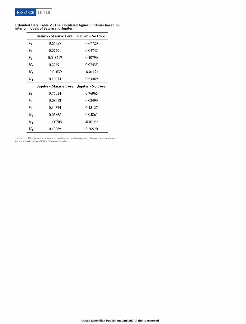
Extended Data Table 2 | The calculated figure functions based oninterior models of Saturn and Jupiter

The values of the figure functions are derived for the two limiting cases of massive core and no-core(continuous density profile) for Saturn and Jupiter.

RESEARCH LETTER

Macmillan Publishers Limited. All rights reserved©2015