1

Satellite views of Pacific chlorophyll variability: comparisons to physical variability, local versus nonlocal influences and links to climate indices

Andrew C. Thomas1, P. Ted Strub2, Ryan Weatherbee1 and Corinne James2

1. School of Marine Sciences, University of Maine, Orono, ME, U.S.A. 2. College of Oceanic and Atmospheric Science, Oregon State University, Corvallis, OR, U.S.A.

ABSTRACT

Concurrent satellite-measured chlorophyll (CHL), sea surface temperature (SST), sea level anomaly (SLA) and model-derived wind vectors from the 13+ year SeaWiFS period September 1997 – December 2010 quantify time and space patterns of phytoplankton variability and its links to physical forcing in the Pacific Ocean. The CHL fields are a metric of biological variability, SST represents vertical mixing and motion, often an indicator of nutrient availability in the upper ocean, SLA is a proxy for pycnocline depths and surface currents while vector winds represent surface forcing by the atmosphere and vertical motions driven by Ekman pumping. Dominant modes of variability are determined using empirical orthogonal functions (EOFs) applied to a nested set of domains for comparison: over the whole basin, over the equatorial corridor, over individual hemispheres at extra-tropical latitudes (> 20o) and over eastern boundary current (EBC) upwelling regions. Strong symmetry exists between hemispheres and the EBC regions, both in seasonal and non-seasonal variability. Seasonal variability is strongest at mid latitudes but non-seasonal variability, our primary focus, is strongest along the equatorial corridor. Non-seasonal basin-scale variability is highly correlated with equatorial signals and the strongest signal across all regions in the study period is associated with the 1997-1999 ENSO cycle. Results quantify the magnitude and geographic pattern with which dominant basin-scale signals are expressed in extra-tropical regions and the EBC upwelling areas, stronger in the Humboldt Current than in the California Current. In both EBC regions, wind forcing has weaker connections to non-seasonal CHL variability than SST and SLA, especially at mid and lower latitudes. Satellite-derived dominant physical and biological patterns over the basin and each sub-region are compared to indices that track aspects of climate variability in the Pacific (the MEI, PDO and NPGO). We map and compare the local CHL footprint associated with each index and those of local wind stress curl, showing the dominance in most areas of the MEI and its similarity to the PDO. Principal estimator patterns quantify the linkage between dominant modes of forcing variability (wind, SLA and SST) and CHL response, comparing local interactions within EBC regions with those imposed by equatorial signals and mapping equatorial forcing on extra-tropical CHL variability.

Corresponding author: A.C. Thomas. Tel.: 207 581 4335 E-mail address: thomas@maine.edu Keywords: Pacific, chlorophyll, sea level, surface temperature, eastern boundary currents, climate indices, satellite data

2

1. Introduction The climatological pattern of surface phytoplankton biomass over the Pacific basin (Fig. 1)

reflects dominant patterns of heating, wind stress and stratification that control the flux of

subsurface nutrients into the euphotic zone. Seasonal variability about this pattern is dominated

by mid-latitude shifts in the location of the transition zone separating oligotrophic subtropical

gyre waters from more productive waters at higher latitudes (Longhurst, 1995; Vantrepotte and

Melin, 2009; Yoder and Kennelly, 2003). Elsewhere, responses to interannual forcing, often of

equatorial origin such as the El Niño Southern Oscillation (ENSO), can be of similar magnitude

or larger than local seasonal cycles (e.g. Chavez et al., 1999; Martinez et al., 2009; Vantrepotte

and Melin, 2011; Yoder and Kennelly, 2003), transmitted through atmospheric teleconnections

(e.g. Chhak and DiLorenzo, 2007; Schwing et al., 2010) and oceanic pathways (e.g. Hormazabal

et al., 2001; Strub and James, 2002c). Along the eastern basin margins, the biologically

productive California and Humboldt eastern boundary current (EBC) upwelling systems respond

rapidly and strongly to basin scale signals imposed from lower latitudes (Carr et al., 2002; Kahru

and Mitchell, 2000) as well as higher latitudes (Freeland et al., 2003; Wheeler et al., 2003). Such

EBC variability is superimposed on more locally controlled variability driven by latitudinally

modulated seasonal wind forcing and heating (Bakun and Nelson, 1991; Thomas et al., 2001b).

The energetic structure and relatively strong time and space gradients of EBCs make them

logical regions to examine oceanic responses to climate-related signals.

Satellite data provide the most systematic views of coupled biological-physical interannual

variability over large spatial scales. Over the Pacific, linkages between chlorophyll (CHL) and

physical variability characterized by sea surface temperature (SST) and sea level anomaly (SLA)

have been described for specific areas and/or time periods (e.g. Carr et al., 2002; Murtugudde et

al., 1999; Signorini and McClain, 2012; Wilson and Adamec, 2001). Other work (Martinez et

al., 2009; Vantrepotte and Melin, 2011) extends these views, quantifying linkages between CHL,

SST and climate-related signals over the entire Pacific. Symmetry between SST patterns in each

hemisphere has been shown (Shakun and Shaman, 2009), however the symmetry of coupled

biological-physical patterns in each hemisphere and the extent to which such basin-scale

variability is reflected in EBC systems remains less well described. Here, we build upon these

previous efforts; examining the full SeaWiFS mission period (13+ years) and concurrent SST

3

and SLA satellite data for dominant patterns over the whole basin and various sub-regions of the

Pacific Ocean. We describe the relative symmetry of patterns in the northern and southern

hemispheres, the projection of equatorial and basin-scale patterns into the EBC regions and the

relationship between satellite-measured variability and three Pacific climate indices. We then

quantify local EBC biological-physical coupling, contrasting it with forcing of EBC regions from

the equatorial zone.

Patterns of atmospheric and hydrographic variability along the Pacific equatorial corridor and

their local biological response are dominated by interannual variability associated with ENSO

events with periods of two to seven years (Philander, 1999), effectively tracked by the

multivariate ENSO index (Wolter and Timlin, 1998). The signature of ENSO is the leading mode

of SST variability in the Pacific (Deser et al., 2010). The oceanic biological implications of

ENSO variability are evident throughout the Pacific and up to global scales (Chavez et al., 2011;

Martinez et al., 2009). Within the Pacific, ENSO signals have their most direct extra-tropical

impact in the two Pacific eastern boundary currents (EBCs), where eastward propagating

equatorial Kelvin waves have a direct connection into the Humboldt Current as a result of

coastline shape and proximity and less direct but still clear connections into the California

Current (Strub and James, 2002a). These excite poleward propagating coastal-trapped waves. In

these EBCs, the arrival of elevated sea levels, a deeper upper mixed layer and warmer, nutrient-

poor surface conditions during an El Niño event means wind-driven coastal upwelling does not

bring nutrient-rich water to the surface, leading to sharply reduced coastal phytoplankton

biomass (Kahru and Mitchell, 2002; Ulloa et al., 2001).

On multi-decadal timescales in the North Pacific, the Pacific Decadal Oscillation (Mantua and

Hare, 2002) serves as an index of oceanic climate variability. Defined as the dominant mode of

surface temperature variability north of 20oN, the PDO is the North Pacific response to

atmospheric forcing by the winter strength of the Aleutian low (Bond and Harrison, 2000) and is

connected to ENSO forcing (Di Lorenzo et al., 2010; Shakun and Shaman, 2009). The PDO is

strongly correlated with merged SST - CHL non-seasonal variability over the Pacific basin

(Martinez et al., 2009) and linked to biological variability across multiple trophic levels

(Anderson and Paitt, 1999; Cloern et al., 2010). Thomas et al. (2009) show positive correlations

4

over a 7-year period for coastal chlorophyll in the northern California Current (41-48oN) and off

Baja California 28-31oN. The second mode of North Pacific SST and SLA variability, the North

Pacific Gyre Oscillation (Di Lorenzo, 2008) describes the relative strength of gyre circulation

and has correlations with salinity and nutrient concentrations in the North Pacific, phytoplankton

biomass in the southern California Current, and is positively correlated to coastal chlorophyll off

the Pacific Northwest and off Baja California (Thomas et al., 2009). It also has links to ENSO

forcing (Di Lorenzo et al., 2010). In the South Pacific, the footprint of the PDO and the NPGO

on biological variability remains poorly described, but both appear to have correlations to coastal

CHL in the Humboldt Current, at least at specific latitudes (Thomas et al., 2009).

Our analyses are shaped by three perspectives: (1) use of surface chlorophyll as the primary

variable of interest; (2) consideration of the Pacific Basin but with its two EBCs as the primary

regions of interest; and (3) use of consistently processed satellite data where possible, in order to

obtain a “synoptic” view of biophysical interactions over the widest and most uniformly sampled

range of spatial scales possible. The SeaWiFS instrument provides over 13 years of basin-scale

coverage of phytoplankton biomass. Temporally coincident missions measured physical

processes that potentially modulate phytoplankton patterns: SST (a metric of surface

stratification, mixing and nutrient availability) and SLA (a metric of pycnocline depth and

current structure). We augment these with model wind stress (wind stress curl: the driver of

Ekman pumping / suction and alongshore wind stress: the driver of coastal upwelling). Against a

background of better known seasonal CHL variability (Vantrepotte and Melin, 2009; Yoder et

al., 2010), our objectives are to relate satellite-derived fields of CHL to fields of SLA, SST and

wind stress in the Pacific Basin in order to: (1) contrast the synoptic modes of variability of CHL

with physical variables, including the degree of symmetry between hemispheres; (2) relate basin-

scale signals to those of the two Pacific EBC regions, comparing them to local forcing; and (3)

relate satellite-derived statistical modes to three indexes of climate variability, the MEI, PDO

and the NPGO. For completeness, we recognize our study areas have links to variability in the

western Pacific basin (Miller et al., 2004) that are not addressed here.

2. Data and Methods

5

SeaWiFS monthly-averaged CHL over the duration of the mission (September 1997 – December

2010) were obtained from the NASA ocean color server. CHL values are the standard NASA

chlorophyll algorithm (O'Reilly et al., 1998), reprocessing version R2010. Instrument difficulties

create three data gaps of 2-4 months duration in 2008 and 2009. At latitudes > ~50o, few data are

available during hemisphere winter months due to darkness. We work with log transformed CHL

values, consistent with previous work showing their underlying distribution (Campbell, 1995).

Even in the monthly means, CHL retrievals at some pixels in this data set have some

suspiciously high values, likely a result of localized failures in atmospheric correction, cloud

edge effects and/or bio-optical algorithm failure in turbid water, creating noisy fields. We reduce

this noise in a series of steps, cognizant of our focus on longer time/space scale signals. Values

greater than 30 mg m-3 were flagged as missing. Data were then log10 transformed and at each

location values greater than the climatological mean plus two standard deviations were also

flagged as missing. Data were transformed back into chlorophyll space and a 3x3 median spatial

operator was then passed over each monthly field twice, and then transformed back into log10

units and the climatological mean at each location was removed. We use two time series, (log

transformed) CHL concentrations with zero mean at each location (retaining seasonality) and

monthly anomalies created by subtracting the climatological months from each year at each

location.

Maps of 1/4 degree SLA gridded from multiple satellites were obtained from AVISO

(http://www.aviso.oceanobs.com). For September 1997 - November 2010, monthly averages

were created from available weekly fields of the AVISO Updated Delayed Time sea level

anomaly product. We extended the SLA time series one month through December 2010 using

“near real time” SLA data for consistency with the other time series. For June 2010 through

December 2010, daily fields of the AVISO Daily Merged Near Real Time SLA data were

averaged into monthly means. The two monthly time series were combined into a single monthly

time series spanning September 1997- December 2010 using a weighted average to smooth the

transition between the Delayed Time and the Near Real Time data. EOFs calculated with and

without the last added month (merged data) were indistinguishable, beyond extending the time

series to match the CHL data. The time average for each point was removed. Subtracting the

climatological months from this time series created anomaly fields.

6

Monthly average fields of optimally interpolated Reynolds SST version 2, OI.v2 (Reynolds et

al., 2002), on a 1o grid were obtained from the Environmental Modeling Center at the National

Weather Service (ftp://ftp.emc.ncep.noaa.gov/cmb/sst/oimonth_v2/). The time average was

removed from each spatial data point. Climatological months were computed for the period

September 1997 - December 2010 and subtracted from the time series to create anomalies.

ECMWF ERA-Interim Project wind data are used. These six-hourly horizontal wind fields from

NCAR’s Data Support Section are used to calculate wind stress and wind stress curl using a

variable drag coefficient (Large et al., 1995), then averaged into monthly values. The time

average for each point was removed. Subtracting the climatological monthly means from these

created anomaly fields. The time series at each location was smoothed using a 3-month boxcar

filter. The monthly means remove variability on the scale of synoptic storms and upwelling

events of several days. As we are primarily interested in quantifying the large-scale, interannual

differences in vertical motion of nutrients beneath the mixed layer driven by Ekman transports

(coastal upwelling and open-ocean Ekman pumping), alternating fluctuations on shorter time

scales will average into the monthly means in a linear fashion. Primary production, however, is

not reversible and so is not a linear process. An analysis of event-scale responses of

phytoplankton to wind forcing is beyond the scope of our large-scale analysis, but must be kept

in mind while interpreting our results. Such a study would require different statistical techniques

and is worthy of a separate investigation.

Data over marginal seas of the Pacific (e.g. the Bering, Okhotsk, Japan, South China, Gulf of

California) are excluded from each spatial field to focus analysis on the Pacific basins and their

EBCs (Fig. 1). The final data set is a concurrent, 160-month time series of CHL, SST, SLA and

wind stress anomalies.

Empirical orthogonal functions (EOFs) isolate dominant modes of satellite-measured variability

over a series of nested study domains. EOFs are empirical in the sense that the space/time

patterns are purely a function of the variance present in the target data set making them sensitive

to the space and time domain of the data set. We exploit this characteristic to compare dominant

7

modes calculated over the whole Pacific basin with those over just the equatorial region (0o +/-

20o), within each higher-latitude hemisphere (20o – 60o) and then within each EBC upwelling

region (Fig. 1). Due to strong, often non-coherent variability in both time and space in these data,

even the dominant modes often capture relatively small percentages of the total variance over

such large regions. These, however, are the dominant coherent time/space patterns in the data

that are the focus of our investigation.

Significance of the resulting EOF modes can be discussed from 3 perspectives; statistical

significance of the modes, relative separation of the eigenvalues of each mode, and the bio-

physical realism of the time/space pattern. First, to examine statistical significance we use the N-

rule approach outlined by Overland and Preisendorfer (1982) to estimate those eigenvalues for

which the geophysical signal exceeds the level of noise within the data. For all the EOFs

calculated here, each of the first 3 modes (we present, at most, the dominant 2) exceeds the noise

level by this criterion. Second, limitations in sampling of the signals in question can mean that

eigenvalues that are very similar may not provide realistic separation of underlying actual

patterns in the data set (Deser et al., 2010; Dommenget and Latif, 2002; North et al., 1982). We

examined each of the first 3 modes of the EOFs we present for separation using the rule of thumb

suggested by North et al. (1982). Of the 24 modes presented, the eigenvalues of all but 3 are

statistically separate from that of the following mode. The 3 questionable modes are each over

the South Pacific and we discuss our interpretation of them when they are presented. Lastly,

caution should be exercised in interpretation of EOF modes as the orthogonality imposed by the

calculation means that even statistically significant modes might not capture real oceanic

variability (Dommenget and Latif, 2002). As the real modes of variability are unknown, this is

difficult to assess. However, we note many similarities, especially at the large scales discussed

here, in the overall space patterns captured by these independently measured, multidisciplinary

EOFs. There are also correlations of the EOF time series both between the independently

measured environmental parameters and to various Pacific climate indices. In addition, for SST

and SLA, time series longer than the SeaWiFS mission examined here are available. EOFs over

these longer periods (not shown) revealed very similar time and space modes to those over our

shorter study period. While not conclusive, these do suggest oceanic biophysical modes rather

than statistical artifacts. Although often noisy and capturing relatively small percentages of the

8

total non-seasonal variance over these large scales, we suggest the EOF modes offer realistic

satellite views of biophysical coupling and its spatial pattern across the Pacific and into the

eastern boundaries.

Direct linkages between physical variability and biological response are quantified using

principal estimator patterns (Davis, 1977). PEPs calculate a linear combination of a set of

predictor fields that explain the greatest amount of variance of a set of estimand data fields. Here,

the EOF modes of alongshore wind stress, SLA and SST are the predictor fields and those of

CHL are the estimand fields (Strub et al., 1990). The PEPs result in paired sets of spatial

patterns, one each for the predictor and CHL field, associated with a single common time series,

with the dominant mode capturing the largest amount of variance. The “skill” of each mode is

expressed as the fraction of the original CHL variance explained by the combined space-time

series, constrained to be some fraction of the dominant modes of EOF variability.

We compare signals evident in the satellite-derived patterns to three climate-related indices of

Pacific atmosphere-ocean variability, the MEI (www.ersl.noaa.gov), the PDO (University of

Washington jisao.washington.edu/pdo/PDO.latest) and the NPGO (courtesy of E. DiLorenzo

from www.o3d.org/npgo).

Significance of correlations between time series, used to quantify similarity, was calculated by

modifying n, the number of months in the time series, to an “effective” degrees of freedom to

account for autocorrelation within the time series. Decorrelation time scales vary among all the

individual signals examined. We calculated decorrelation time scales of those with the most

obvious longer-term features. Results ranged from 4 to 8 months, with most in the 4-5 month

range. For simplicity, we assume a 6-month autocorrelation time scale and reduce degrees of

freedom by dividing n by 6 for all signals. Only those correlations significant at the 95% level

are presented and only the stronger of these are discussed.

3. Results and Discussion 3.1 Dominant seasonal chlorophyll patterns

9

EOFs of monthly CHL fields (Fig. 2) present the dominant patterns of seasonal variability

superimposed on the climatological mean (Fig. 1). These are similar to results of previous studies

(Antoine et al., 2005; Lewis et al., 1988; Longhurst, 1995; Messie and Radenac, 2006; Thomas

et al., 2001b; Vantrepotte and Melin, 2009; Yoder and Kennelly, 2003) but included here to

provide the background against which non-seasonal patterns can be compared. They also

highlight the seasonal symmetry between the two hemispheres and their respective EBC regions

and document the complete SeaWiFS mission not included in previous studies. Over the entire

basin and in the California and Humboldt EBC regions, the first 2 modes capture most of the

seasonal structure (47%, 41%, and 32% of total variance, respectively) with relatively weak

interannual differences over their 13+ year time series. The third modes (not shown) have strong

non-seasonal signals, analyzed separately in the following sections. Time and space patterns in

the first two modes of the entire basin calculated over the 13+ years are generally similar to those

evident over the Pacific in a global EOF analysis of a 4-year period (1998-2001) presented by

Yoder and Kennelly (2003), indicative of both the temporal and spatial stability of the overall

seasonal structure.

Over the whole basin (Fig. 2a), Mode 1 is dominated by mid latitude annual cycles, maximum in

hemisphere winter, representing seasonal shifts in the location of the frontal transition zone

separating oligotrophic subtropical gyre waters from more productive waters at higher latitudes

(Fig. 1). Highest latitudes in both hemispheres (> about 45o) have the opposite sign, creating

summer maxima. Together, these capture the transition from a nutrient limited to a light limited

annual cycle (Dandonneau et al., 2004). Patterns at low latitudes (< 20o) are relatively weak

except along the far eastern margin in the vicinity of wind-jets at Central America’s mountain

gaps (Chelton et al., 2000) and in the Peru upwelling region, consistent with previously shown

EBC seasonality (Echevin et al., 2008; Thomas et al., 2009). Mode 2 is 3 months out of phase

with Mode 1 (maxima in May and November), allowing the combination of the two modes to

describe a smooth meridional shift of the mid-latitude extrema. This mode also includes maxima

with different signs at the Central American mountain gaps, in the Southern Ocean and in the

EBC upwelling regions off North America and Chile. The most prominent features are a basin-

wide zonal positive band at ~ 10oN paired with a weaker, less extensive, negative zonal

maximum at ~ 10oS describing CHL maxima in early summer of each hemisphere. Spatially,

10

these track climatological patterns of wind stress curl associated with positive vertical velocity

(Risien and Chelton, 2008; Talley et al., 2011).

In EBC regions (Fig. 2b), mode 1 maxima are present along each coastal upwelling region,

maximum in each hemisphere’s summer, accompanied by weaker offshore maxima in the

hemisphere’s winter. These are ~ 1 month earlier in the California Current than those over the

whole basin and the Humboldt Current, consistent with analyses of shorter records (Thomas et

al., 2001b). Elevated coastal concentrations are strongest/widest in the Pacific Northwest and off

Baja California in the California Current and off central Peru and central-southern Chile in the

Humboldt Current, weakest and narrow off northern Chile and reversed along southern

California. Mode 2 captures additional seasonality, primarily in the upwelling regions of the

southern California Current and Peru. Opposite-phased maxima occur at higher latitudes,

especially central Chile. The April (positive) maximum in the time series in both EBCs initiates

elevated concentrations early in the summer season off Baja and southern California (Espinosa-

Carreon et al., 2004) and extends the summer high values later in the season off Peru. The

September and November negative maxima describe weak late summer high latitude peaks in the

California Current and stronger spring peaks off Chile, respectively.

3.2 Basin-scale non-seasonal variability

Removing the climatological monthly fields from each time series produces the non-seasonal

signals highlighting interannual variability, the primary focus of this study. In contrast to

seasonal signals, the two dominant modes of non-seasonal CHL variability (23% of total non-

seasonal variance) over the basin (Fig. 3a) are centered on the equatorial region. The first mode

CHL spatial pattern is highlighted by a strong westward pointing “arrowhead” shaped positive

feature, centered at the equator, maximum ~ 160oE to 160oW. Three fingers of elevated

variability extend eastward from this maximum, one north of the equator at ~ 10oN extending

east and continuous with elevated variability off Central America, one at the equator that extends

east to ~ 140oW and the third tracking southeast into the South Pacific to ~ 20oS at 120oW.

These resemble features isolated as both multi-year trend and non-stationary seasonality by

Vantrepotte and Mélin (2011). Their relation to seasonality is evident here as the northern and

11

southern “fingers” overlay almost exactly the positive/negative zonal bands of the Mode 2

seasonal CHL pattern (Fig. 2a). Smaller positive areas are along the coast of Peru, Mexico and

off Southern California, with weak positive regions at higher (> 40o) latitudes. The strongest

negative pattern is in the far western equatorial Pacific north of New Guinea. The time series is

dominated by strong negative values during the 1997-1998 El Niño (Chavez et al., 1999;

McPhaden, 1999; Strub and James, 2002a). Thereafter, 3 periods are evident, generally positive

in 1999-2001, negative in 2002-2007 and positive again in 2007-2009. In Mode 2, the strongest

features reflect additional variability associated with the same features as Mode 1: negative

values in the western warm pool are centered at ~ 160oE extending northeast along the Mode 1

northern finger, a relative minimum also extends along the southern edge of the southern Mode 1

finger. Strong positive patterns are associated with features off Central America, in phase with

features in the EBC upwelling regions, strongest close to the coast. The Mode 2 time series is

strongly negative in 1997 and early 1998, weakens relatively slowly and becomes positive in

2001, remaining so until 2008. Together, these two modes describe a large region of negative

CHL anomalies across the equatorial Pacific during the 1997-1998 El Niño period with positive

CHL anomalies in the west. The positive anomalies spread eastward as the time series become

positive first for Mode 1, followed by Mode 2. During 2008-2010, Mode 1 reflects conditions

that switched from La Niña to El Niño and back.

SLA variability (Fig. 3b), a tracer of changes in upper mixed layer thickness and nutricline depth

(Polovina et al., 1995; Wilson and Adamec, 2001), is also predominantly focused on equatorial

regions. In mode 1, a tongue of positive values extends from ~ 170oE eastward across the basin

at the equator, continuous with a broad region along the eastern low latitude margins. West of

170oE, equatorial patterns are strongly negative from ~ 20oN to 10oS, with weaker negative

regions extending into subtropical central basins at mid latitudes. The time series for this mode is

dominated by strong positive values in 1997-1998 during the El Niño. It switches to negative

values from mid 1998 until 2002, with positive events in 2002-03 and 2009-10 associated with

weaker El Niño events and obviously mirrors the CHL signal. SLA mode 2 isolates additional

variability dominated by low latitude processes, strongly negative at low latitudes from the

western side of the basin to ~ 110oW, with a weaker negative centered at ~ 45oN in the NE

Pacific. This time series mirrors the CHL Mode 2 signal, positive in mid 1998 during later stages

12

of the ENSO cycle. Thereafter, its amplitude is weaker and mainly negative from 2001 to early

2010.

Basin-wide EOF modes of non-seasonal SST (not shown) are substantially similar to SLA,

dominated by equatorial signals with maximum amplitudes during the 1997-1998 El Niño,

patterns shown and discussed in previous work (Deser et al., 2010; Messie and Chavez, 2011).

SLA and SST EOF time series are highly correlated across the first 2 modes (Table 1). EOFs of

basin-scale non-seasonal wind stress curl (not shown), however, are dominated by patterns over

the Southern Ocean and neither their space nor time patterns resemble those of CHL, SST or

SLA.

Comparisons between the CHL patterns and those of SLA (and SST) in mode 1 (Fig. 3) show the

canonical association of lower (higher) CHL values with elevated (decreased) SLA, indicative of

a thicker (thinner) mixed layer over the eastern basins and main basin gyres where signals are

weaker (Wilson and Adamec, 2002). In equatorial regions where the signals are strong, CHL

maxima appear most closely associated with the edges of SLA features, suggesting links to

changes in the equatorial current structure (Wilson and Adamec, 2001). Space patterns in the two

second modes are less similar and appear to capture different phases of transition in the ENSO

cycle (McPhaden, 1999), an observation supported by slight differences in the timing of the 1998

maxima. The strong link between non-seasonal temporal CHL variability and satellite-measured

physical variability evident in Fig. 3 is quantified in the correlations between modes 1 and 2

across CHL, SLA and SST (Table 1).

The extent of dominance of basin-scale non-seasonal modes by equatorial variability is

investigated by calculating separate EOFs over a spatial domain restricted to +/- 20o of the

equator (see Fig. 1). EOFs for CHL, SST and SLA in this equatorial corridor (not shown) have

patterns that are essentially identical to those for the whole basin in the equatorial region of

spatial overlap. Equatorial EOF time series are strongly correlated (all > 0.94) with those of their

basin-scale counterpart (Table 1) in both modes 1 and 2.

3.3 Extra-tropical patterns, symmetry and relationships to basin-scale signals

13

Removing the equatorial signal isolates variability occurring at higher latitudes allowing

comparisons of the degree to which hemispheres vary symmetrically and the extent to which

higher-latitude variability tracks that at the equator. The dominant modes of CHL, SLA and SST

EOFs calculated separately over 20-60o latitude in each hemisphere (see Fig. 1) are presented in

Fig. 4. In the northern hemisphere, mode 1 spatial patterns are generally similar among

chlorophyll, SLA and SST, positive in eastern portions of the basin and negative over the central

basin, strongest between 160o and 180oW. Their respective time series are well correlated (Table

2). In the southern hemisphere, strongest CHL variability is centered between 80o-100oW and

130o-160oW at mid latitudes. Variability south of 40oS (over the Southern Ocean) is weak except

for a small region west of New Zealand. Mode 1 spatial patterns of SLA and SST are similar,

strongest and positive over the Southern Ocean (100o-160oW), and negative, although with

differences in latitude, over the eastern subtropical gyre and around New Zealand. Their time

series are correlated (Table 2). These modes, however, are not correlated with that of CHL. CHL

mode 1 is better related to mode 2 of both SLA and SST (Table 2), whose variance is also

centered at mid latitudes between 130o and 160oW.

For each of these southern hemisphere EOF decompositions (Fig. 4), very similar eigenvalues

(% variance explained) over the dominant 2-3 modes call into question their separability (North

et al., 1982). We evaluate their separation and validity using a number of approaches. CHL

mode 1 (Fig. 4a, 10% of total variance) is not statistically separate from mode 2 (not shown).

Recalculation of this EOF following increased smoothing of the initial monthly CHL fields (not

shown) produced very similar space patterns and highly correlated time series over the dominant

3 modes, each of which was separate by North et al.’s (1982) rule of thumb. We take this as

evidence that CHL mode 1 (Fig. 4a) is likely separate, but with statistics hidden by the relatively

noisy biological signal. For both SLA and SST we have access to additional data with which to

compare our modes. Computation of an SLA EOF over the southern hemisphere region for the

full period of AVISO data availability (October 1992 – December 2010, i.e. 5 additional years)

produces dominant modes (not shown) strongly resembling those presented and time series that

are highly correlated over the time period of overlap (0.95 and 0.98 respectively). Each of the

first 3 modes in this longer time series decomposition is statistically separate (North et al., 1982),

14

evidence that our presented modes are also separate. A similar approach with SST data made use

of a higher time and space resolution data set (1/4 degree, daily) with which we calculated EOFs

over the period January 1982 – December 2010 (i.e. ~ 16 years of additional data). The first 3

modes of this decomposition are clearly separate by North et al.’s criteria. The first 2 modes have

spatial patterns similar to those in Fig. 4c with correlated time series (0.76, 0.71, for modes 1 and

2, respectively). Patterns resemble those with strongest variance over the Pacific presented by

Messié and Chavez (2011). We take these as evidence that the presented modes are separate.

How symmetric is non-seasonal variability in the two hemispheres? Spatially, taking into

account the longitudinal difference in the eastern basin margin of each hemisphere, Fig. 4 shows

symmetry between the northern and southern hemispheres in spatial pattern for SST, consistent

with previous results (Shakun and Shaman, 2009) and also for SLA, less so for CHL. Positive

regions in the eastern portions of the basins mirror each other, expanding westward at lower and

higher latitudes. Negative regions trend from mid latitudes in the east towards lower latitudes in

the west. Temporally (Table 2), while correlations between modes 1 of each hemisphere of each

measurement are statistically significant, only that of SST (0.72) appears similar over the whole

study period (Fig. 4c, bottom). Obvious differences in timing of specific events in CHL and SLA

(Fig. 4a and b) are evident reducing their inter-hemisphere correlations. Respective second

modes are not well correlated.

To what degree does dominant variability at higher latitudes reflect those calculated over the

whole basin? This is relevant because many climate indices (e.g. the NPGO, PDO and North

Pacific Oscillation) are defined by variability confined to higher latitudes in the North Pacific

and the basin signals are strongly correlated to equatorial signals (Table 1). In the northern

hemisphere, mode 1 space patterns of CHL, SLA and SST (Fig. 4) have clear similarity to their

counterparts in the whole basin EOFs (Fig. 3, SST not shown). Strong correlation of their

respective time series (Table 2), indicate that dominant northern hemisphere non-equatorial

patterns reflect those over the basin and in the equatorial corridor. Despite these correlations, an

obvious difference between the time series in Fig. 3 and those of Fig. 4 is the reduced relative

strength of the 1997-1998 El Niño signal. At higher latitudes, variability later in the time series is

15

often of equal, or greater, magnitude. Correlations between southern hemisphere and whole basin

CHL and SLA are significant but weak, however those of SST are relatively strong (Table 2).

3.4 Eastern boundary current variability

Satellite-measured non-seasonal CHL variability in the Pacific EBC upwelling regions is

relatively well documented over specific times and regions (Carr et al., 2002; Kahru and

Mitchell, 2001, 2002; Thomas et al., 2003). Here we focus on dominant coherent variability over

the entire EBC domains, their relative symmetry in the two hemispheres and their similarity to

concurrent physical signals. The first EOF modes of CHL variability (Fig. 5a, 18% and 16% of

the total variance in the California and Humboldt regions, respectively) show the strongest

signals over the study period in both regions are negative anomalies during the 1997-1998 El

Niño, strongest in the Humboldt Current. Thereafter, CHL variability is relatively weak in the

Humboldt, stronger in the California region, where there are positive values in 2002, negative

peaks in early 2004 and 2005, and a prolonged positive period over the last 5 years, maximum in

2008. In the California Current, values are strongest offshore of the Southern California Bight in

the Ensenada frontal region where the main jet of the California Current turns eastward

(Espinosa-Carreon et al., 2004; Thomas and Strub, 1990) and along the Oregon coast. Weakest

patterns are in offshore regions off northern California and Baja California, and along the

northern California coast (~ 38-40oN). In the Humboldt Current, patterns are strongest along the

entire Peru coast and in a narrow coastal strip extending into northern Chile, consistent with the

strong El Niño impacts (Carr et al., 2002; Thomas et al., 2001a) in these regions. Patterns are

relatively strong off central Chile (~30-40oS), weakest in the offshore region off southern Peru –

northern Chile and reversed at latitudes > ~ 45oS where influences of Southern Ocean forcing

become stronger (Montecino et al., 2006). CHL time series of the two regions are weakly

correlated (Table 3) largely on the strength of the same strong El Niño signal in the first 12

months (Fig. 5). Weaker features in 2002, 2004 and 2005 appear out of phase. Correlations

recalculated excluding the first 16 months (the strong ENSO), are not significant.

Comparisons of these CHL patterns to first modes of SLA and SST variability (Fig. 5b and c)

show that large positive SLA and SST values are associated with the negative CHL signals

16

during the El Niño period of 1997-1998 in both EBCs. SLA and SST in both EBCs are primarily

negative for 1999 – 2002, the La Niña period, becoming positive in the period 2003-2006 in the

California Current, while in the Humboldt Current time series are weak. All four SST and SLA

time series are well correlated with each other (Table 3), indicating physical symmetry and

suggesting common forcing. Their negative correlation with CHL variability, most strongly in

the Humboldt Current, is consistent with previous work showing strong coupling between the

physical and biological processes in these region on interannual time scales (e.g. Carr et al.,

2002; Chavez et al., 2002; Legaard and Thomas, 2006; Ulloa et al., 2001). One pattern that is

consistently different between the two EBC regions in these three data sets is their latitudinal

distribution (Fig. 5), weighted heavily towards the lowest latitudes in the Humboldt Current but

relatively evenly weighted across the full latitudinal extent of the California Current. This

difference reflects the lower latitudes included in the Humboldt Current, connecting the EBC

wave guide directly to the El Niño signal. Substantial latitudinal propagation and travel around

coastal features are required for this signal to arrive in the California system.

Alongshore wind stress (AWS, defined positive northward in both hemispheres) represents direct

local forcing of coastal upwelling and enhanced summer CHL in the EBC regions. The dominant

non-seasonal mode in each EBC region (Fig. 5d) has strong short-period temporal variability at

highest latitudes, symptomatic of winter storm systems, resulting in a spatial mismatch between

dominant non-seasonal wind forcing and the other satellite-measured variables (Fig. 5a-c).

Correlations between the non-seasonal AWS and the ocean variables are weak or insignificant

(Table 3). Of interest, however, are strong positive (negative) anomalies during El Niño in the

California (Humboldt) Current revealing poleward (downwelling-favorable) AWS anomalies at

latitudes > ~35oN in the California Current and off central Chile (30-40oS). This supports an

atmospheric connection and contribution to the negative CHL and positive SLA and SST

anomalies at the higher latitudes. This pattern is reversed or absent in both systems at lower

latitudes, reaffirming the role of poleward propagating SLA signals in creating the low latitude

EBC anomalies.

How similar are dominant CHL patterns within the EBC regions to those over the whole basin?

Spatially, California Current patterns (Fig. 5) are similar to those in this region calculated over

17

the whole basin (Fig. 3) and their respective time series are correlated (Table 3). Dominant

patterns in the Humboldt Current have spatial similarities to both modes of basin-wide CHL

variability (Fig. 3) and are temporally correlated with both (r=0.52 and 0.65 respectively), each

stronger than those in the California Current (emphasizing the Humboldt Current’s more direct

equatorial connection). Over the time window analyzed here, EBC CHL interannual variability is

strongly related to that over the whole basin, contributing to the symmetry between systems and

suggestive of common responses to climate signals of equatorial origin.

3.5 Satellite-measured variability: relationships to climate indices

The strongest non-seasonal signal over the 13-year study period in most of the satellite-measured

time series presented above is the 1997-1998 El Niño, associated with positive anomalies of SLA

and SST and negative anomalies in CHL. The MEI (Fig. 6), designed to track ENSO equatorial

variability (Wolter and Timlin, 1998), is strongly correlated with the dominant mode of non-

seasonal variability of each satellite signal in each of the separate study areas (Table 4), most

strongly (as expected) in the equatorial and whole basin regions for SST and SLA. ENSO

impacts on equatorial SST, SLA and CHL patterns are well documented (McClain et al., 2002;

Murtugudde et al., 1999), as are satellite views of CHL in the two EBC regions (Carr et al.,

2002; Chavez et al., 2002; Kahru and Mitchell, 2000; Thomas et al., 2001a). The MEI tracks the

dominant mode of merged CHL-SST non-seasonal variability over the whole Pacific (Martinez

et al., 2009) and explains ~ 21% and 35% of mode 1 CHL variability in the California and

Humboldt systems, respectively, over the complete SeaWiFS mission period. In the southern

and northern extra-tropics, the MEI accounts for 25% and 32%, respectively, of mode 1 CHL

variance (Table 4), similar to its impact on the EBCs. The difference is that the ENSO has a

stronger effect on the northern hemisphere extra-tropical band than on its EBC, while its direct

connection to South America delivers a greater impact on the southern hemisphere EBC.

The first EOF of SST north of 20oN (Fig. 4) represents the purely satellite-data analogue of the

PDO (Fig. 6) over the 13-year study period. Not surprisingly, the space pattern looks

indistinguishable from that of the PDO (see http://jisao.washington.edu/pdo/) and its time series

is highly correlated (Table 4). The North Pacific EOFs of SLA and CHL (Fig. 4) are similar to

18

that of SST, their time series are highly correlated (Table 2), and each is more strongly related to

the PDO than the MEI (Table 4), the only region where this is true, reflecting their North Pacific

emphasis. Chhak et al. (2009) discuss the linkage between SLA, SST and the PDO in the North

Pacific. Satellite time series over both the whole basin and the equatorial region are correlated

with the PDO, consistent with previous results (Martinez et al., 2009) and indicative of

connections between equatorial dynamics (ENSO) and North Pacific physical variability

discussed by many authors (Di Lorenzo et al., 2010; Newman et al., 2003; Strub and James,

2002c) but expanded here to include a biological component. Restricted to variability in the

California Current, correlations to the PDO are strong for SLA and SST, present but weaker for

chlorophyll. In the southern hemisphere, the PDO is correlated to SST over the extra-tropics but

not the EBC (Table 4), similar to the strong correlation between the dominant modes of SST in

the northern and southern extra-tropics (Table 2 and Figure 4). Do these satellite data suggest a

PDO-equivalent extra-tropical SST mode in the southern hemisphere? If so, does it resemble the

PDO and is it connected to ENSO? Figures 4 and 6 and Tables 2 and 4 provide affirmative

answers. The dominant mode of satellite SST in the southern extra-tropics is similar (not

identical) to its northern counterpart; their correlation represents a common 52% of their

variance. Both are correlated with the MEI and PDO (Table 4) and basin-scale SST variability

(Table 2), consistent with decadal-scale SST linkages into both extra-tropical hemispheres from

ENSO forcing (Shakun and Shaman, 2009).

Defined as the second mode of SLA variability in the northeast Pacific, Di Lorenzo et al. (2008)

suggest that the NPGO is the oceanic expression of the atmospheric forcing associated with the

North Pacific Oscillation that in turn is connected to ENSO variability (Di Lorenzo et al., 2010).

The NPGO represents low frequency gyre circulation variability with links to upwelling strength

and biological variables in the North Pacific (Cloern et al., 2010; Di Lorenzo, 2008). Quantified

by satellite data over our 13-year time window, the second mode of SLA in the North Pacific is

weakly correlated with the NPGO (Table 4), as are several other modes calculated here. In

general, our satellite-defined dominant modes are not closely correlated with the NPGO, a

finding possibly related to the differing spatial domains used to isolate variability, the relatively

short 13-year time window of the satellite data used here, and/or noise in the satellite signals (Di

Lorenzo, pers. comm. 2011).

19

By definition, time series from EOF modes represent coherent variability taken collectively

across the entire input study region. Location-specific variability may or may not be closely

related. We quantify the biological footprint of the climate indices by mapping their correlations

to non-seasonal CHL at each location (Fig. 7). The strongest correlations are with the MEI

across low latitudes (Fig. 7a), positive in the far western warm pool as discussed by Messie and

Radenac (2006) and Christian et al. (2004), and negative along the rest of the equatorial corridor.

Negative values extend to higher latitudes in the eastern basin along the coasts of Peru and

Mexico. MEI impacts on both subtropical gyres are positive. Higher resolution views into the

EBC regions show strong negative correlations continuous in a narrow band next to the Baja

California coast, a broad negative region off southern and central California extending > 500km

offshore and weaker negative values along the Oregon and Washington coasts. Positive

correlations offshore of Baja California are consistent with a bloom of chlorophyll observed

during the 1997-1998 El Niño in this region (Kahru and Mitchell, 2000), apparently robust over

a 13+ year correlation. The MEI footprint in the Humboldt Current is strong off Peru

equatorward of ~ 15oS extending > 500km offshore, spatially continuous with the equatorial

pattern evident in the whole basin view. South of this, the footprint is weaker, but still negative

next to the coast to ~ 22oS in the narrow coastal upwelling region (Thomas et al., 2001a).

Negative values expand more broadly offshore south of ~ 28oS, a region of increased eddy and

filament activity (Montecino et al., 2006). The footprint of the PDO (Fig. 7b), both at the basin

scale and into these EBC regions, is similar to, but weaker than, that of the MEI, consistent with

the similarity in their time series over this 13-year period (Fig. 6) and connections in their

forcing (Di Lorenzo et al., 2010; Shakun and Shaman, 2009).

The imprint of the NPGO on CHL (Fig. 7c) is generally of the opposite sign, has differences in

spatial pattern and is weaker than both the MEI and PDO at most locations. The strongest feature

is positive in regions along the northern and southern flanks of the tongue of elevated equatorial

chlorophyll values evident in Fig. 1, with many similarities to features evident in the dominant

mode of basin CHL variability (Fig. 3). Their time series are correlated (Table 4). A major

difference between NPGO patterns and those of the MEI and PDO is the lack of any strong

footprint along the equator. One explanation is relative differences in the equatorial connections

20

of these indices: direct/immediate for the MEI and strong for the PDO with its links to the ENSO

cycle, but more indirect and weaker for the NPGO, a high latitude oceanic signal imposed by the

wind forcing patterns of the NPO (Chhak and DiLorenzo, 2007; Di Lorenzo et al., 2010). In the

EBC regions, CHL correlations with the NPGO are weak, strongest (positive) off southern Baja

California and northern Washington. Adjacent to most EBC coastline regions, weak correlations

are primarily negative.

We contrast the CHL footprint of these climate indices with that of vertical motions in the water

column imposed by Ekman pumping due to local non-seasonal wind stress curl (WSC, Fig. 7d).

In EBC regions, WSC contributes to upwelling (Abbott and Barksdale, 1991), affects higher

trophic levels (Rykaczewski and Checkley, 2008) and is subject to interannual variability

imposed by El Niño events (Halpern, 2002). Canonical relationships between Ekman pumping

and biological response have positive (negative) curl in the northern (southern) hemisphere

driving upwelling and increases in CHL. This relationship is clearly present in each EBC system.

(Immediately adjacent to the South American coast, however, the ECMWF wind vectors do not

adequately represent WSC due to in the influence of the Andes on spectral atmospheric models.)

Over the whole basin, this link is weaker. Over broad regions of the eastern North Pacific and

into the Gulf of Alaska, weak positive correlations link positive curl with increased CHL, but

this is not true over the subtropical gyre and is strongly reversed in the equatorial corridor within

10o of the equator. This reversal at low latitudes is mirrored in the Southern Hemisphere where

positive curl is associated with increased CHL anomalies. The implications are that in these low

latitudes and the subtropical gyres, at the time and space scales addressed here, interannual

variability in local WSC plays a weaker role in modulating CHL than other processes captured

by the climate indices and satellite-measured SLA and SST and that these processes are

associated with WSC signals opposite to those that cause upwelling.

3.6 Physical-biological coupling: within EBC regions

PEPs quantify local EBC time and space coupling between dominant CHL modes of variability

and physical modes, characterized here by AWS (τ), SLA and SST. In the California Current

(Fig. 8a-c), differences in the spatial patterns of forcing and CHL responses can be interpreted in

21

comparison to previously viewed time/space patterns. The AWS space pattern is strongest and

positive at higher latitudes, decreasing sharply at ~ 35oN, with weaker and reversed winds in the

Southern California Bight and off Baja California, consistent with the geography of wind stress

(Bakun and Nelson, 1991) that shows maxima off northern California and weaker, but more

persistent upwelling winds off Baja California. The SLA pattern is weighted higher towards the

coast and at lower latitudes, similar to SLA and SST in the Humboldt Current (Fig. 8e,f) and

suggestive of coastally trapped signals arriving from low latitudes. California Current SST has

no space pattern, implying a simple EBC-wide connection between high SST and low CHL.

Poleward AWS and positive SST are coupled with similar negative CHL patterns; the main

differences are extensions of lower CHL right to the California coast, throughout the Southern

California Bight and continuous along Baja California coast in response to higher SST. CHL

coupled to local SLA (Fig. 8b) is most similar to the CHL footprint of the MEI (Fig. 7),

suggesting closer links to equatorial signals. Each California Current time series shows positive

anomalies during the 1997-1998 El Niño period. Alongshore wind stress is positive northward,

so association of positive times series with a positive wind spatial pattern indicates anomalously

strong northward, or weaker equatorward (upwelling-favorable) winds during the El Niño.

Thereafter, a number of events are recognizable from previous studies. Enhanced CHL

concentrations linked to colder SSTs are evident in late 2001 and 2002, associated with an

anomalous advection of colder, nutrient-rich subarctic waters into the northern California

Current (Freeland et al., 2003; Thomas et al., 2003; Wheeler et al., 2003). In the first half of

2005, all three time series switch abruptly from strongly positive to weakly negative, the coupled

response to delayed seasonal upwelling (Barth et al., 2007).

In the Humboldt Current (Fig. 8d-f), SLA and SST have similar spatial patterns strongly

weighted to low latitudes. Each is dominated by positive 1997-1998 El Niño signals and each has

considerably more “skill” driving non-seasonal CHL than AWS. Both are linked to similar CHL

patterns, with maximum negative anomalies off Peru and coastal regions of northern Chile and

again off central Chile 30-40oS. After the El Niño signal, the time series of both SLA and SST

are weaker than those in the California Current. This, and the increased skill of SLA and SST

PEPs in the Humboldt Current are likely due to more direct linkages to equatorial signals and

relatively weaker local processes that influence non-seasonal CHL variability. The AWS pattern

22

is dominated by variability at the highest latitudes where winds are dominated by Southern

Ocean storms; non-seasonal AWS variability over lower latitudes is comparatively weak. CHL

variability, however, is strongest off Peru (Fig. 5a) and this mismatch likely explains the lower

“skill” of this PEP.

3.7 Physical-biological coupling: equatorial links to regional chlorophyll variability

EOFs and PEPs of variability at higher latitudes and in the EBC regions (Figs. 4, 5 and 8) are

dominated by 1997-1998 El Niño signals, well correlated to the MEI (Table 4) and clearly linked

to equatorial variability. Here we contrast the views of “local” coupling (Fig. 8) to those of non-

local forcing of CHL by satellite-measured physical signals in the equatorial corridor. PEPs of

equatorial SLA and SST generated substantially similar CHL patterns and time series, as

expected from the strong correlation of dominant equatorial SLA and SST EOF modes (Table 1).

For brevity we show only those of SLA forcing CHL.

PEPs of equatorial SLA (and SST, not shown) forcing EBC CHL are shown in Fig. 9a and b.

Equatorially forced California Current CHL PEP patterns are substantially similar to “local”

coupling (Fig. 8) south of ~ 38oN, but differ from those produced by local wind and SST (Fig. 8a

and c) off Oregon and Washington. This suggests patterns at these higher latitudes have stronger

links to local (or non-equatorial) wind forcing and associated SST response, consistent with links

to NE Pacific atmospheric variability in this region (Barth et al., 2007; Freeland et al., 2003;

Strub and James, 2002b). Their joint time series correlate with the MEI (0.75), but with a 1-2

month lag. In the Humboldt Current (Fig. 9b), equatorially forced CHL patterns are almost

identical to those forced locally (Fig. 8e and f), and their joint time series correlation to the MEI

is 0.75 with no lag, both consistent with a more direct connection to low latitude signals.

PEPs of equatorial SLA (and SST, not shown) forcing northern and southern hemisphere extra-

tropical CHL variability (Fig. 9c and d) quantify coupling between equatorial signals (the

satellite-derived analogues to the MEI) and biology at extra-tropical latitudes. These show

biological patterns similar to those in Fig. 4: elevated equatorial SLA is associated with a)

increased CHL within the central gyres and b) decreased CHL along the eastern rim of the basin,

23

strongest off south-central California, into the Gulf of Alaska and off Chile. Equatorial SLA (and

SST) patterns driving these CHL patterns, however, differ. Northern Hemisphere CHL is

associated with forcing focused right along the equator, strongest in the central Pacific. The joint

time series is synchronous with the MEI during 1997-1998 and lags it by ~2 months thereafter

with an overall correlation of 0.81. Southern Hemisphere CHL is associated with equatorial SLA

(and SST) patterns with a basin-wide zonal gradient, more similar to those evident in Mode 2 of

the basin-scale SLA EOF (Fig. 3) and suggestive of later, transitional stages of the ENSO cycle.

The joint PEP time series is weakly (but significantly) correlated with the MEI (0.43) at a lag of

1 month. These differences point to more direct coupling of North Pacific CHL to equatorial

signals with maximum coupling in each hemisphere linked to different phases of the ENSO

cycle.

4.0 Summary and Conclusions Both seasonal and non-seasonal biological and physical variability in the Pacific measured by 13

years of concurrent satellite data (CHL, SLA and SST) have strong symmetry about the

equatorial region. Seasonal patterns are strongest at mid latitudes and non-seasonal patterns are

focused along the equatorial corridor.

Dominant modes of non-seasonal EOFs calculated over the whole basin and the equatorial (0o

+/- 20o) region, are strongly correlated between regions and all variables, indicative of close

biological-physical coupling and equatorial domination of Pacific variability. Wind EOFs are

dominated by Southern Ocean variability and poorly correlated with these signals.

Non-seasonal variability and biological-physical coupling from each of the study regions is

strongly dominated by the ENSO signals of 1997-1999, defined well by both basin-scale and

equatorial SLA and SST EOF modes. Away from the equator, this interaction is strongest along

the two Pacific EBC regions, extending into the higher latitudes in the Humboldt Current and

present but weaker into higher latitudes of California Current, where variability in years after the

1997-1999 ENSO signal is also strong. Dominant modes of SLA, SST and CHL in each study

region are most significantly correlated with the MEI, and less so with the PDO except in the

North Pacific. Links to the NPGO are weak in these data.

24

The spatial footprints of the MEI and PDO on non-seasonal chlorophyll patterns across the

Pacific and in the EBC regions are similar, consistent with their coupled forcing, maximum

along the equatorial corridor and also important in broad areas along the coasts of both North and

South America. The CHL footprint of non-seasonal wind stress curl is evident in the EBC

regions but in other regions, especially near the equator, the relationship is opposite to that which

would increase primary production, suggesting that other non-seasonal forcing dominates in

these regions. We realize that these forcing mechanisms are not independent. Through the

ENSO, the MEI is linked to the PDO and to the NPGO through the influence of atmospheric

forcing on SST (and SLA) patterns at higher latitudes. Each also has connections to basin-scale

wind stress curl patterns and alongshore wind stress in the EBC regions.

Overall, the two EBCs show a gradation from control of CHL at lower latitudes by SLA to

control by winds at higher latitudes. In the California Current, PEPs show coupling between

CHL and local wind, SLA and SST, weakest for wind at low latitudes; time series of SLA and

SST indicate equatorial forcing. In the Humboldt Current, PEPs show wind has less interaction

with chlorophyll interannual variability than SST and SLA, pointing to more direct connections

of SLA and SST to equatorial signals. PEPs also show the direct interaction of equatorial SLA

and SST variability on EBC and higher latitude CHL, confirming the above links in EBC

regions. The PEPs show that northern hemisphere extra-tropical CHL lags equatorial signals by

~ 2 months and is most closely linked to El Niño anomalies in the central equatorial Pacific

while southern hemisphere extra-tropical CHL response is weaker, not lagged, and more closely

linked to transitional equatorial patterns of the ENSO cycle.

Lastly, these time series are short by climate standards; requiring merging with additional ocean

color missions to address decadal changes (Antoine et al., 2005; Martinez et al., 2009), and too

short to address anthropogenic influences on oceanographic variability (Henson et al., 2010).

They do, however, demonstrate the extent to which a single consistent mission a) can quantify

and reveal patterns of large-scale variability related to climate and b) reflect variability tracked

by major climate indices. They provide spatial details in CHL coupling to SLA and SST patterns

unavailable from in situ data. Lags between the MEI and PEP time series connecting equatorial

25

SLA and California Current CHL spatial distributions highlight their potential predictive

capabilities and emphasizes the need to continue these satellite observations into the future.

Acknowledgments

We thank the NASA SeaWiFS project team for providing the ocean color satellite data, AVISO,

NOAA/NWS/NCEP and NCAR for access to SLA, SST and wind data products, respectively,

and those people/organizations (referenced in the text) that make the various climate indices

available. Funding for this work was provided by NSF as part of the U.S. GLOBEC program to

ACT (OCE-0814413, OCE-0815051) and PTS (OCE-0815007). Additional support for PTS was

provided by the NASA Ocean Surface Topography Science Team (NNX08AR40G). This is

contribution XXX of the U.S. GLOBEC program.

26

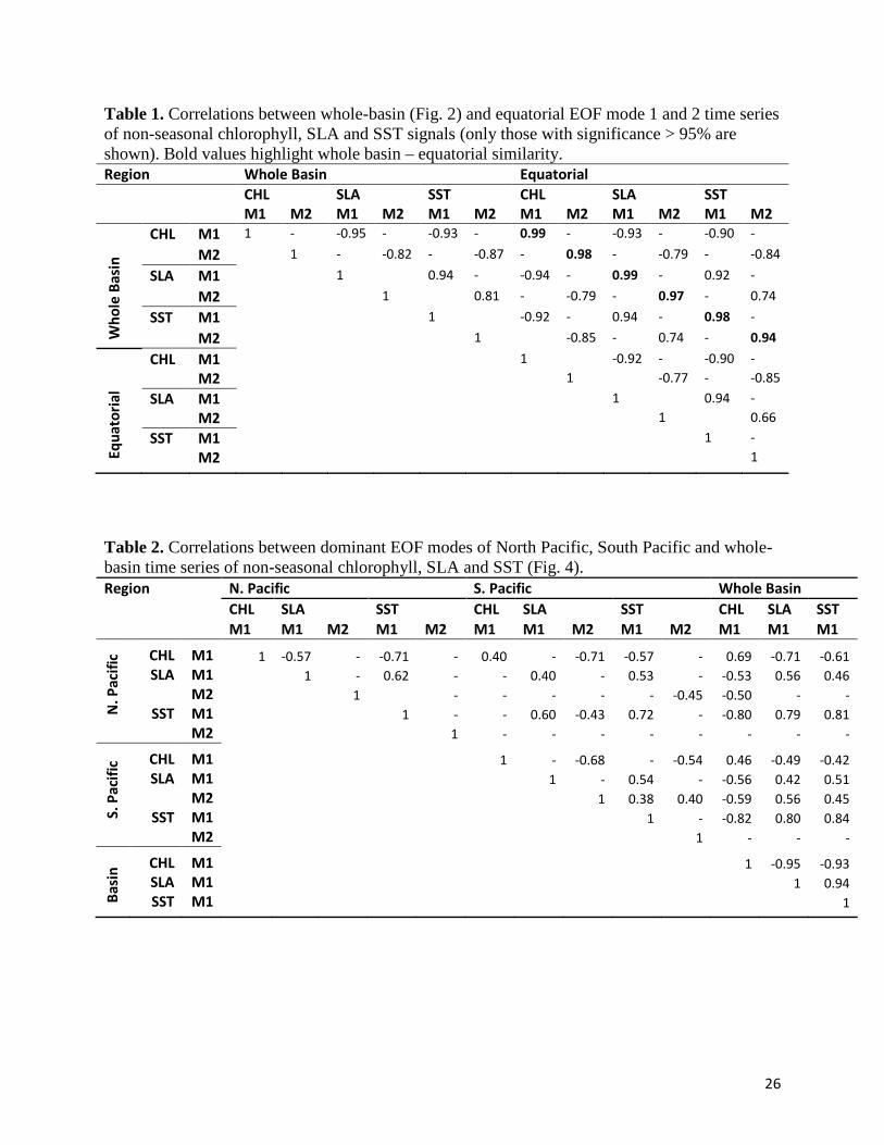
Table 1. Correlations between whole-basin (Fig. 2) and equatorial EOF mode 1 and 2 time series of non-seasonal chlorophyll, SLA and SST signals (only those with significance > 95% are shown). Bold values highlight whole basin – equatorial similarity. Region Whole Basin Equatorial CHL SLA SST CHL SLA SST M1 M2 M1 M2 M1 M2 M1 M2 M1 M2 M1 M2

Who

le B

asin

CHL M1 1 - -0.95 - -0.93 - 0.99 - -0.93 - -0.90 - M2 1 - -0.82 - -0.87 - 0.98 - -0.79 - -0.84

SLA M1 1 0.94 - -0.94 - 0.99 - 0.92 - M2 1 0.81 - -0.79 - 0.97 - 0.74

SST M1 1 -0.92 - 0.94 - 0.98 - M2 1 -0.85 - 0.74 - 0.94

Equa

toria

l

CHL M1 1 -0.92 - -0.90 - M2 1 -0.77 - -0.85

SLA M1 1 0.94 - M2 1 0.66

SST M1 1 - M2 1

Table 2. Correlations between dominant EOF modes of North Pacific, South Pacific and whole- basin time series of non-seasonal chlorophyll, SLA and SST (Fig. 4). Region N. Pacific S. Pacific Whole Basin

CHL SLA SST CHL SLA SST CHL SLA SST M1 M1 M2 M1 M2 M1 M1 M2 M1 M2 M1 M1 M1

N. P

acifi

c CHL M1 1 -0.57 - -0.71 - 0.40 - -0.71 -0.57 - 0.69 -0.71 -0.61 SLA M1 1 - 0.62 - - 0.40 - 0.53 - -0.53 0.56 0.46

M2 1 - - - - - -0.45 -0.50 - - SST M1 1 - - 0.60 -0.43 0.72 - -0.80 0.79 0.81

M2 1 - - - - - - - -

S. P

acifi

c CHL M1 1 - -0.68 - -0.54 0.46 -0.49 -0.42 SLA M1 1 - 0.54 - -0.56 0.42 0.51

M2 1 0.38 0.40 -0.59 0.56 0.45 SST M1 1 - -0.82 0.80 0.84

M2 1 - - -

Basi

n CHL M1 1 -0.95 -0.93 SLA M1 1 0.94 SST M1 1

27

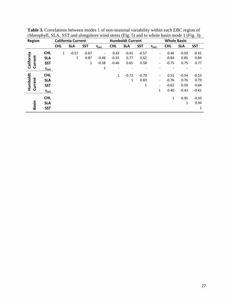
Table 3. Correlations between modes 1 of non-seasonal variability within each EBC region of chlorophyll, SLA, SST and alongshore wind stress (Fig. 5) and to whole basin mode 1 (Fig. 3). Region California Current Humboldt Current Whole Basin CHL SLA SST τ(as) CHL SLA SST τ(as) CHL SLA SST

Calif

orni

a Cu

rren

t CHL 1 -0.57 -0.67 - 0.43 -0.41 -0.57 - 0.46 -0.50 -0.41 SLA 1 0.87 -0.46 -0.55 0.77 0.62 - -0.84 0.85 0.84 SST 1 -0.38 -0.46 0.65 0.58 - -0.75 0.75 0.77 τ(as) 1 - - - - - - -

Hum

bold

t Cu

rren

t CHL 1 -0.72 -0.70 - 0.52 -0.54 -0.53 SLA 1 0.83 - -0.76 0.76 0.79 SST 1 - -0.62 0.59 0.64 τ(as) 1 0.40 -0.43 -0.41

Basi

n

CHL 1 -0.95 -0.93 SLA 1 0.94 SST 1

28

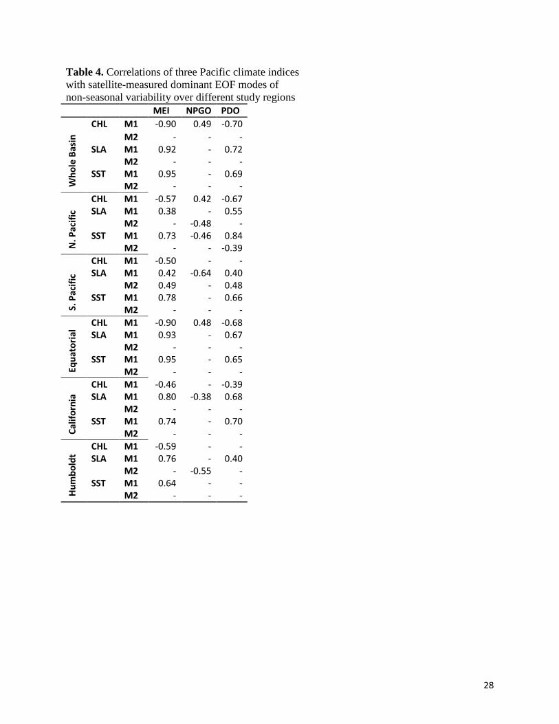
Table 4. Correlations of three Pacific climate indices with satellite-measured dominant EOF modes of non-seasonal variability over different study regions MEI NPGO PDO

Who

le B

asin

CHL M1 -0.90 0.49 -0.70 M2 - - - SLA M1 0.92 - 0.72

M2 - - - SST M1 0.95 - 0.69

M2 - - -

N. P

acifi

c

CHL M1 -0.57 0.42 -0.67 SLA M1 0.38 - 0.55

M2 - -0.48 - SST M1 0.73 -0.46 0.84

M2 - - -0.39

S. P

acifi

c

CHL M1 -0.50 - - SLA M1 0.42 -0.64 0.40

M2 0.49 - 0.48 SST M1 0.78 - 0.66

M2 - - -

Equa

toria

l CHL M1 -0.90 0.48 -0.68 SLA M1 0.93 - 0.67

M2 - - - SST M1 0.95 - 0.65

M2 - - -

Calif

orni

a

CHL M1 -0.46 - -0.39 SLA M1 0.80 -0.38 0.68

M2 - - - SST M1 0.74 - 0.70

M2 - - -

Hum

bold

t

CHL M1 -0.59 - - SLA M1 0.76 - 0.40

M2 - -0.55 - SST M1 0.64 - -

M2 - - -

29

Figure Captions Fig. 1. The study area showing major geographic locations, climatological mean chlorophyll concentrations and the geographic boundaries of sub-regions (equatorial corridor +/- 20o, North Pacific and South Pacific 20o-60o, California and Humboldt Currents) among which regional variability is compared. Marginal seas were not included in the analysis. Fig. 2. Seasonal CHL variability characterized by the first two modes (mode 1 top, mode 2 bottom) of an EOF decomposition of monthly chlorophyll fields over a) the whole basin and b) the Pacific eastern boundary current regions. The 13-year time series of each mode (mode 1 solid, mode 2 dashed, in b the Humboldt is red), which have only weak interannual variability, is simplified to its climatological annual cycle to highlight the seasonality captured in each mode. The percent of total variance isolated by each mode is indicated. Fig. 3. The first two modes of an EOF decomposition over the whole basin of monthly non-seasonal a) CHL concentrations and b) SLA, showing their respective space patterns, associated time series (CHL solid line, SLA dotted line) and the percent of total variance explained by each over the study period. Fig. 4. The dominant modes of variability from EOF decompositions (calculated separately) over the North Pacific and the South Pacific study regions (20o-60o latitude, see Fig. 1) for each of a) CHL, b) SLA and c) SST (the first 2 modes of SLA and SST in the southern hemisphere), showing those modes that have the most similar space pattern and most strongly correlated time series. Below each are their respective time series (bold line: northern hemisphere, dotted line: southern hemisphere mode 1, thin solid line: southern hemisphere mode 2) and the % variance explained by each mode. Fig. 5. The first modes of EOF decompositions of CHL, SLA, SST and alongshore wind stress over a 500km wide region encompassing the main upwelling regions of the California and Humboldt Current EBC regions, showing the space pattern of each and their respective time series (solid line: California, dotted line: Humboldt). The percent variance each mode explains is given above the time series. Fig. 6. Time series of 3 Pacific climate indices, the MEI, PDO and NPGO, over the study period. Fig. 7. Projection correlations that map the footprint of the a) MEI, b) PDO, c) NPGO and d) non-seasonal local wind stress curl (WSC) variability onto non-seasonal CHL at each grid location over the entire basin and in each EBC region. EBC values are the same as those over the basin but at higher spatial resolution and a different color scale to improve coastal details. The MEI, PDO and NPGO are a single time series correlated to CHL at each CHL grid location. In 7d, CHL was re-mapped to the coarser resolution wind product grid and correlations of local wind stress curl with local CHL formed at each location. Fig. 8. Principal estimator patterns of CHL in the (a-c) California and (d-f) Humboldt EBC regions predicted by each of AWS (τ), SLA and SST, showing the pairs of predictor and estimand (CHL) space patterns, their common time series (solid line: California, dashed line:

30

Humboldt), the percent of original predictor variance used by the PEP and the percent of the estimand (CHL) original total variance explained (“skill” of the PEP). Fig. 9. Principal estimator patterns of CHL in the (a) California and (b) Humboldt EBC regions and the (c) North Pacific and (d) South Pacific, each predicted by equatorial SLA, showing the pairs of predictor (SLA) and estimand (CHL) space patterns, the common time series (black) that modulate each, the percent of predictor (SLA) variance used by the PEP and the percent of the estimand (CHL) variance explained (“skill” of the PEP). Superimposed (blue) on each time series is the MEI (Fig. 6) as an aid for comparison.

31

References Abbott, M.R., Barksdale, B., 1991. Phytoplankton pigment patterns and wind forcing off central

California. Journal of Geophysical Research 96, 14649-14667. Anderson, P.J., Paitt, J.F., 1999. Community reorganization in the Gulf of Alaska following

ocean climate regime shift. Marine Ecology Progress Series 189, 117-123. Antoine, D., Morel, A., Gordon, H.R., Banzon, V.F., Evans, E.H., 2005. Bridging ocean color

observations of the 1980s and 2000s in search of long-term trends Journal of Geophysical Research 110, doi:10.1029/2004JC002620.

Bakun, A., Nelson, C.S., 1991. The seasonal cycle of wind-stress curl in subtropical eastern boundary current regions. Journal of Physical Oceanography 21, 1815-1834.

Barth, J.A., Menge, B.A., Lubchenco, J., Chan, F., Bane, J.A., Kirincich, A.R., McManus, M.A., Nielsen, K.J., Pierce, S.D., Washburn, L., 2007. Delayed upwelling alters nearshore coastal ocean ecosystems in the northern California current. Proceedings of the National Academy of Sciences 104, 3719-3724.

Bond, N.A., Harrison, D.E., 2000. The Pacific Decadal Oscillation, air-sea interaction and central north Pacific winter atmospheric regimes. Geophysical Research Letters 27, 731-734.

Campbell, J.W., 1995. The lognormal distribution as a model for bio-optical variability in the sea. Journal of Geophysical Research 100, 13,237-213,254.

Carr, M.E., Strub, P.T., Thomas, A.C., Blanco, J.L., 2002. Evolution of 1996-1999 La Nina and El Nino conditions off the western coast of South America: A remote sensing perspective. Journal of Geophysical Research 107, doi:10.1029/2001JC001183.

Chavez, F.P., Messié, M., Pennington, J.T., 2011. Marine primary production in relation to climate variability and change. Annual Review of Marine Science 3, 227-260, doi:210.1146/annurev.marine.010908.163917.

Chavez, F.P., Pennington, J.T., Castro, C.G., Ryan, J.P., Michisaki, R.P., Schlining, B., Walz, P., Buck, K.R., McFadyen, A., Collins, C.A., 2002. Biological and chemical consequences of the 1997-1998 El Niño in central California waters. Progress in Oceanography 54, 205-232.

Chavez, F.P., Strutton, P.G., Friederich, C.E., Feely, R.A., Feldman, G.C., Foley, D.C., McPhaden, M.J., 1999. Biological and chemical response of the equatorial Pacific Ocean to the 1997-98 El Nino. Science 286, 2126-2131.

Chelton, D.B., Freilich, M.H., Esbensen, S.K., 2000. Satellite observations of the wind jets off the Pacific coast of Central America. Part I: Case studies and statistical characteristics. Monthly Weather Review 128, 1993-2018.

Chhak, K., DiLorenzo, E., 2007. Decadal variations in the California Current upwelling cells. Geophysical Research Letters 34, doi:10.1029/2007GL030203.

Chhak, K.C., Di Lorenzo, E., Schneider, N., Cummins, P.F., 2009. Forcing of low-frequency ocean variability in the northeast Pacific. Journal of Climate 22, 1255-1276.

Christian, J.R., R. Murtugudde, J. Ballabrera-Poy, McClain, C.R., 2004. A ribbon of dark water: phytoplankton blooms in the meanders of the Pacific North Equatorial Countercurrent Deep-Sea Reseach II 51, 209-228.

Cloern, J.E., Hieb, K.A., Jacobson, T., Sansó, B., Di Lorenzo, E., Stacey, M.T., Largier, J.L., Meiring, W., Peterson, W.T., Powell, T.M., Winder, M., Jassby, A.D., 2010. Biological

32

communities in San Francisco Bay track large-scale climate forcing over the North Pacific. Geophysical Research Letters 37, doi:10.1029/2010GL044774.

Dandonneau, Y., Deschamps, P.-Y., Nicolas, J.-M., Loisel, H., Blanchot, J., Montel, Y., Thieuleux, F., Becu, G., 2004. Seasonal and interannual variability of ocean color and composition of phytoplankton communities in the North Atlantic, equatorial Pacific and South Pacific. Deep-Sea Research II 51, 303-318.

Davis, R.E., 1977. Techniques for Statistical Analysis and Prediction of Geophysical Fluid Systems. Geophysical and Astrophysical Fluid Dynamics 8, 245-277.

Deser, C., Alexander, M.A., Xie, S.-P., Phillips, A.S., 2010. Sea surface temperature variability: patterns and mechanisms. Annual Review of Marine Science 2, 115-143.

Di Lorenzo, E., Cobb, K.M., Furtado, J.C., Schneider, N., Anderson, B.T., Bracco, A., Alexander, M.A., Vimont, D.J., 2010. Central Pacific El Niño and decadal climate change in the North Pacific Ocean. Nature Geoscience 3, doi:10.1038/NGEO1984.

Di Lorenzo, E., Schneider, N., Cobb, K. M., Chhak, K, Franks, P. J. S., Miller, A. J., McWilliams, J. C., Bograd, S. J., Arango, H., Curchister, E., Powell, T. M. and Rivere, P., 2008. North Pacific Gyre Oscillation links ocean climate and ecosystem change. Geophysical Research Letters 35, doi:10.1029/2007GL032838.

Dommenget, D., Latif, M., 2002. A cautionary note on the interpretation of EOFs. Journal of Climate 15, 216-225.

Echevin, V., Aumont, O., Ledesma, J., Flores, G., 2008. The seasonal cycle of surface chlorophyll in the Peruvian upwelling system: a modelling study. Progress in Oceanography 79, 167-176.

Espinosa-Carreon, T.L., Strub, P.T., Beier, E., Ocampo-Torres, F., Gaxiola-Castro, G., 2004. Seasonal and interannual variability of satellite-derived chlorophyll pigment, surface height, and temperature off Baja California. Journal of Geophysical Research 109, doi:10.1029/2003JC002105.

Freeland, H.J., Gatien, G., Huyer, A., Smith, R.L., 2003. Cold halocline in the northern California Current: An invasion of subarctic water. Geophysical Research Letters 30, doi:10.1029/2002GL016663.

Halpern, D., 2002. Offshore Ekman transport and Ekman pumping off Peru during the 1997-1998 El Nino. Geophysical Research Letters 29, 10.1029/2001GL014097.

Henson, S.A., Sarmiento, J.L., Dunne, J.P., Bopp, L., Doney, S.C., John, J., Beaulieu, C., 2010. Detection of anthropogentic climate change in satellite records of ocean chlorophyll and productivity. Biogeosciences 7, 621-640.

Hormazabal, S., Shaffer, G., Letelier, J., Ulloa, O., 2001. Local and remote forcing of sea surface temperature in the coastal upwelling system off Chile. Journal of Geophysical Research 106, 16657-16671.

Kahru, M., Mitchell, B.G., 2000. Influence of the 1997-98 El Nino on the surface chlorophyll in the California Current. Geophysical Research Letters 27, 2937-2940.

Kahru, M., Mitchell, B.G., 2001. Seasonal and nonseasonal variability of satellite-derived chlorophyll and colored dissolved organic matter concentration in the California Current. Journal of Geophysical Research 106, 2517-2529.

Kahru, M., Mitchell, B.G., 2002. Influence of the El Nino-La Nina cycle on satellite-derived primary production in the California Current. Geophysical Research Letters 29, doi:10.1029/2002GL014963.

33

Large, W.G., Morzel, J., Crawford, G.B., 1995. Accounting for surface wave distortion of the marine wind profile in low-level ocean storms wind measurements. Journal of Physical Oceanography 25, 2959-2971.

Legaard, K., Thomas, A.C., 2006. Spatial patterns in seasonal and interannual variability of chlorophyll and surface temperature in the California Current. Journal of Geophysical Research 111, doi:10.1029/2005JC003282.

Lewis, M.R., N. Kuring, Yentsch, C., 1988. Global patterns of ocean transparency: Implications for the new production of the open ocean. Journal of Geophysical Research 93, 6847-6856.

Longhurst, A., 1995. Seasonal cycles of pelagic production and consumption. Progress in Oceanography 36, 77-167.

Mantua, N.J., Hare, S.R., 2002. The Pacific Decadal Oscillation. Journal of Oceanography 58, 35-44.

Martinez, E., Antoine, D., D'Ortenzio, F., Gentili, B., 2009. Climate-driven basin-scale decadal oscillations of oceanic phytoplankton. Science 326, 1253-1256.

McClain, C.R., Christian, J.R., Signorini, S.R., Lewis, M.R., Asanuma, I., Turk, D., Dupouy-Douchement, C., 2002. Satellite ocean-color observations of the tropical Pacific Ocean. Deep-Sea Research Part Ii-Topical Studies in Oceanography 49, 2533-2560.

McPhaden, M.J., 1999. Genesis and evolution of the 1997-98 El Nino. Science 283, 950-954. Messie, M., Chavez, F., 2011. Global modes of sea surface temperature variability in relation to

regional climate indices. Journal of Climate 24, 4314-4331. Messie, M., Radenac, M.-H., 2006. Seasonal variability of the surface chlorophyll in the western

tropical Pacific from SeaWiFS data. Deep-Sea Research 53, 1581-1600. Miller, A.J., Chai, F., Chiba, S., Moisan, J.R., Neilson, D.J., 2004. Decadal-scale climate and

ecosystem interactions in the North Pacific Ocean. Journal of Oceanography 60, 163-188. Montecino, V., Strub, P.T., Chavez, F.P., Thomas, A., Tarazona, J., Baumgartner, T., 2006. Bio-

physical interactions off western South America, in: Robinson, A.R., Brink, K.H. (Eds.), The Global Coastal Ocean Interdisciplinary regional studies and syntheses. Harvard university Press, Cambridge pp. 329-390.

Murtugudde, R.G., Signorini, S.R., Christian, J.R., Busalacchi, A.J., McClain, C.R., Picaut, J., 1999. Ocean color varability of the tropical Indo-Pacific basin observed by SeaWiFS during 1997-1998. Journal of Geophysical Research 104, 18,351-318,366.

Newman, M., Compo, G.P., Alexander, M.A., 2003. ENSO-forced variability of the Pacific Decadal Oscillation. Journal of Climate 16, 3853-3857.

North, G.R., Bell, T.L., Cahalan, R.F., Moeng, F.J., 1982. Sampling errors in the estimation of empirical orthogonal functions. Monthly Weather Review 110, 699-706.

O'Reilly, J.E., Maritorena, S., Mitchell, B.G., Siegel, D.A., Carder, K.L., Garver, S.A., Kahru, M., McClain, C., 1998. Ocean color chlorophyll algorithms for SeaWiFS. Journal of Geophysical Research 103, 24937-24953.

Overland, J.E., Preisendorfer, R.W., 1982. A significance test for principal components applied to a cyclone climatology. Monthly Weather Review 110, 1-4.

Philander, S.G., 1999. A review of tropical ocean-atmosphere interactions. Tellus 51, 71-90. Polovina, J.J., Mitchum, G.T., Evans, G.T., 1995. Decadal and basin-scale variation in mixed

layer depth and the impact on biological production in the central and North Pacific, 1960-88. Deep-Sea Research 42, 1701-1716.

34

Reynolds, R.W., N.A. Rayner, T.M. Smith, D.C. Stokes, Wang, W., 2002. An improved in situ and satellite SST analysis for climate Journal of Climate 15, 1609-1625.

Risien, C.M., Chelton, D.B., 2008. A global climatology of surface wind and wind stress curl fields from eight years of QuikSCAT scatterometer data. Journal of Physical Oceanography 38, 2379-2413.

Rykaczewski, R.R., Checkley, D.M., 2008. Influence of ocean winds on the pelagic ecosystem in upwelling regions. Proceedings of the National Academy of Sciences of the United States of America 105, 1965-1970.

Schwing, F.B., Mendelssohn, R., Bograd, S.J., Overland, J.E., Wang, M., Ito, S., 2010. Climate change, teleconnection patterns, and regional processes forcing marine populations in the Pacific. Journal of Marine Systems 79, 245-257.

Shakun, J.D., Shaman, J., 2009. Tropical origins of North and South Pacific decadal variability. Geophysical Research Letters 36, 10.1029/2009gl040313.

Signorini, S.R., McClain, C.R., 2012. Subtropical gyre variability as seen from satellites. Remote Sensing Letters 3, 471-479.

Strub, P.T., James, C., 2002a. The 1997-1998 oceanic El Nino signal along the southeast and northeast Pacific boundaries - an altimetric view. Progress in Oceanography 54, 439-458.

Strub, P.T., James, C., 2002b. Altimeter-derived surface circulation in the large-scale NE Pacific Gyres. Part 1. seasonal variability. Progress in Oceanography 53, 163-183.

Strub, P.T., James, C., 2002c. Altimeter-derived surface circulation in the large-scale NE Pacific Gyres. Part 2: 1997-1998 El Nino anomalies. Progress in Oceanography 53, 185-214.

Strub, P.T., James, C., Thomas, A.C., Abbott, M.R., 1990. Seasonal and nonseasonal variability of satellite-derived surface pigment concentration In the California Current. Journal of Geophysical Research 95, 11501-11530.

Talley, L.D., Pickard, G.L., Emery, W.J., Swift, J.H., 2011. Descriptive Physical Oceanography: An Introduction, 6th ed. Elsevier, London.

Thomas, A.C., Blanco, J.L., Carr, M.E., Strub, P.T., Osses, J., 2001a. Satellite-measured chlorophyll and temperature variability off northern Chile during the 1996-1998 La Nina and El Nino. Journal of Geophysical Research 106, 899-915.

Thomas, A.C., Brickley, P., Weatherbee, R., 2009. Interannual variability in chlorophyll concentrations in the Humboldt and California current systems. Progress in Oceanography 83, 386-392.

Thomas, A.C., Carr, M.E., Strub, P.T., 2001b. Chlorophyll variability in eastern boundary currents. Geophysical Research Letters 28, 3421-3424.

Thomas, A.C., Strub, P.T., 1990. Seasonal and interannual variability of pigment concentrations across a California current frontal zone. Journal of Geophysical Research 95, 13023-13042.

Thomas, A.C., Strub, P.T., Brickley, P., 2003. Anomalous satellite-measured chlorophyll concentrations in the northern California Current in 2001-2002. Geophysical Research Letters 30, doi: 10.1029/2003GL017409.

Ulloa, O., Escribano, N., Hormazabal, S., Quinones, R.A., Gonzalez, R.R., Ramos, M., 2001. Evolution and biological effects of the 1997-98 El Nino in the upwelling ecosystem off northern Chile. Geophysical Research Letters 28, 1591-1594.

Vantrepotte, V., Melin, F., 2009. Temporal variability of 10-year global SeaWiFS time-series of phytoplankton chlorophyll a concentration. ICES Journal of Marine Science 66, 1547-1556.

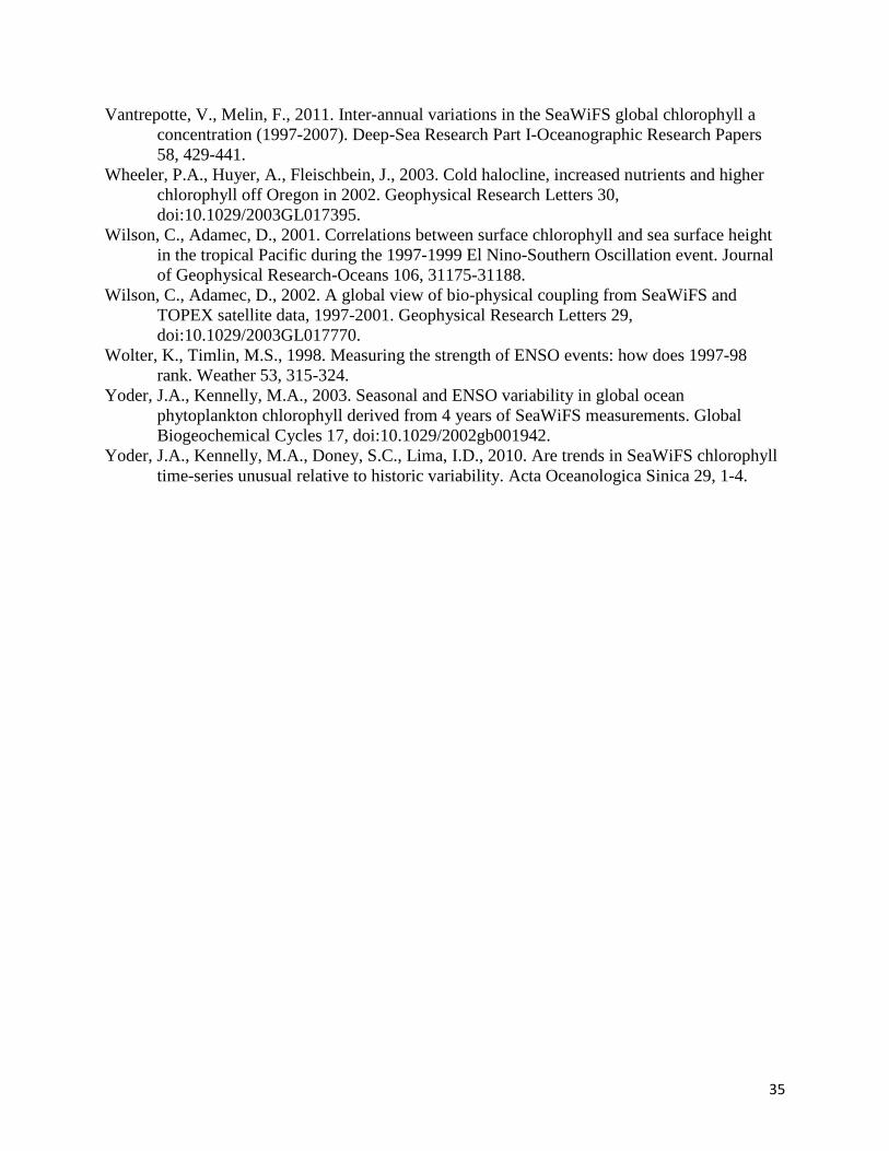
35

Vantrepotte, V., Melin, F., 2011. Inter-annual variations in the SeaWiFS global chlorophyll a concentration (1997-2007). Deep-Sea Research Part I-Oceanographic Research Papers 58, 429-441.

Wheeler, P.A., Huyer, A., Fleischbein, J., 2003. Cold halocline, increased nutrients and higher chlorophyll off Oregon in 2002. Geophysical Research Letters 30, doi:10.1029/2003GL017395.

Wilson, C., Adamec, D., 2001. Correlations between surface chlorophyll and sea surface height in the tropical Pacific during the 1997-1999 El Nino-Southern Oscillation event. Journal of Geophysical Research-Oceans 106, 31175-31188.

Wilson, C., Adamec, D., 2002. A global view of bio-physical coupling from SeaWiFS and TOPEX satellite data, 1997-2001. Geophysical Research Letters 29, doi:10.1029/2003GL017770.

Wolter, K., Timlin, M.S., 1998. Measuring the strength of ENSO events: how does 1997-98 rank. Weather 53, 315-324.

Yoder, J.A., Kennelly, M.A., 2003. Seasonal and ENSO variability in global ocean phytoplankton chlorophyll derived from 4 years of SeaWiFS measurements. Global Biogeochemical Cycles 17, doi:10.1029/2002gb001942.

Yoder, J.A., Kennelly, M.A., Doney, S.C., Lima, I.D., 2010. Are trends in SeaWiFS chlorophyll time-series unusual relative to historic variability. Acta Oceanologica Sinica 29, 1-4.

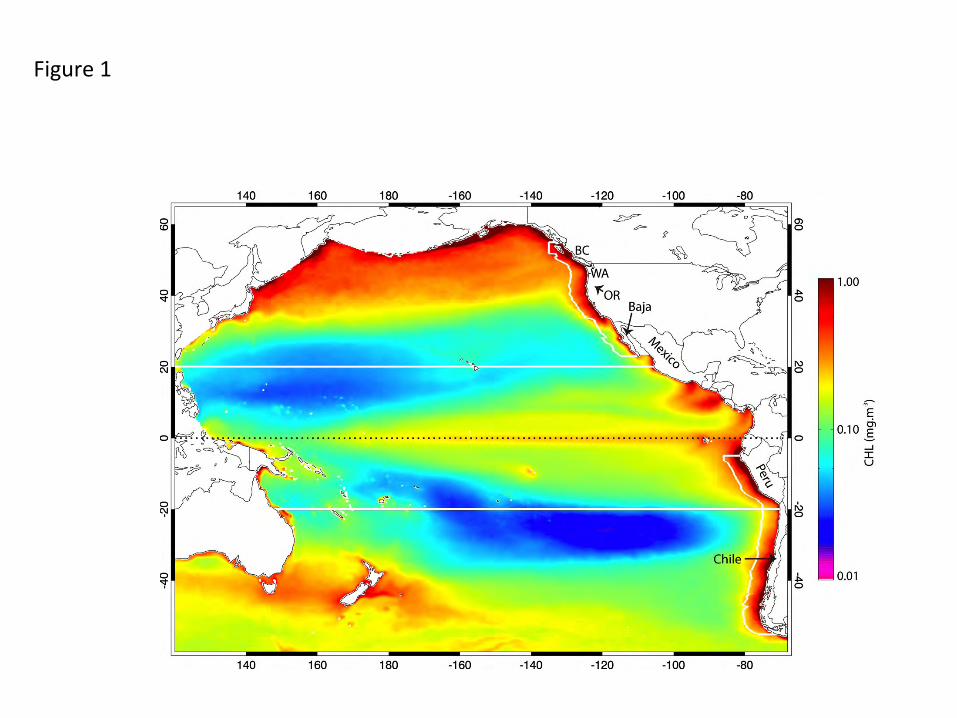
Figure  1  

Figure  2  

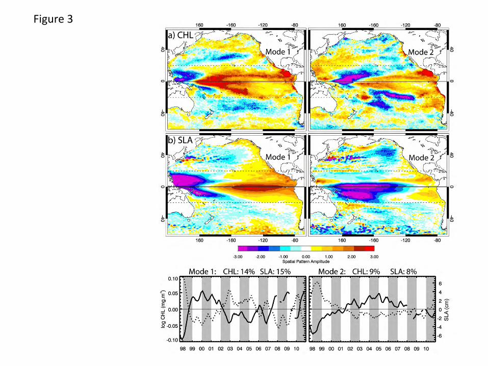
Figure  3  

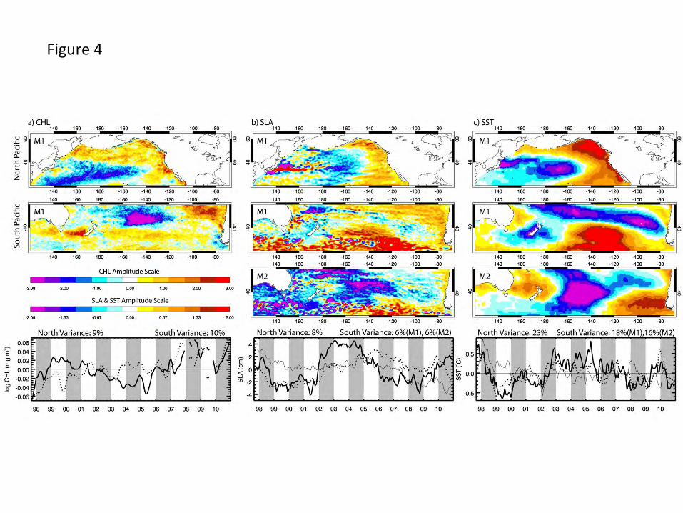
Figure  4  

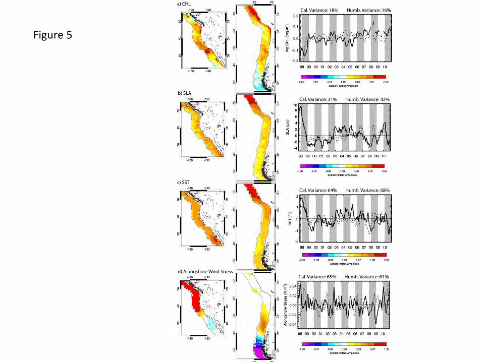
Figure  5  

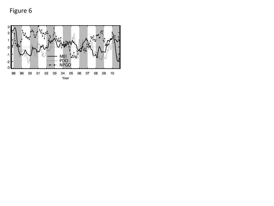
Figure  6  

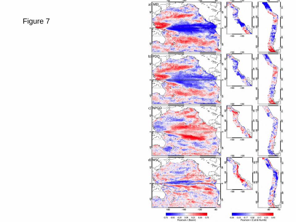
Figure 7

Figure  8  

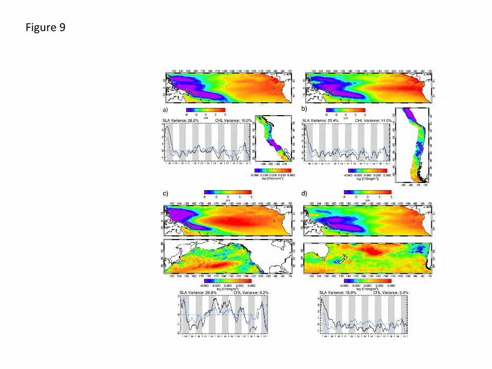
Figure  9