SASEG 6A -- Two-Sample t-Tests

(Fall 2015)

Sources (adapted with permission)-

T. P. Cronan, Jeff Mullins, Ron Freeze, and David E. Douglas Course and Classroom Notes

Enterprise Systems, Sam M. Walton College of Business, University of Arkansas, Fayetteville

Microsoft Enterprise Consortium

IBM Academic Initiative

SAS® Multivariate Statistics Course Notes & Workshop, 2010

SAS® Advanced Business Analytics Course Notes & Workshop, 2010

Microsoft® Notes

Teradata® University Network

Copyright © 2013 ISYS 5503 Decision Support and Analytics, Information Systems; Timothy Paul

Cronan. For educational uses only - adapted from sources with permission. No part of this publication

may be reproduced, stored in a retrieval system, or transmitted, in any form or by any means, electronic,

mechanical, photocopying, or otherwise, without the prior written permission from the author/presenter.

2

Recall the study in the previous chapter by students in Ms. Chao’s statistics class. The board of education

set a goal of having their graduating class scoring on average 1200 on the SAT. The students then went

about seeing if the school district had met its goal by drawing a sample of 80 students at random. The

conclusion was that it was reasonable to assume that the mean of all magnet students was, in fact 1200.

However, an argument had arisen among the boys and the girls in planning the project about whether

boys or girls scored higher. Therefore, they also collected information on gender to test for differences.

3

Objectives Analyze differences between two population means

using the t Test task.

Verify the assumptions of a two-sample t-test.

Perform a one-sided test.

3

4

Test Score Data Set, Revisited

4

3

Before you start the analysis, examine the data to verify that the assumptions are valid.

The assumption of independent observations means that no observations provide any information about

any other observation you collect. For example, measurements are not repeated on the same subject.

This assumption can be verified during the design stage.

The assumption of normality can be relaxed if the data are approximately normally distributed or if

enough data are collected. This assumption can be verified by examining plots of the data.

There are several tests for equal variances. If this assumption is not valid, an approximate t-test can

be performed.

If these assumptions are not valid and no adjustments are made, the probability of drawing incorrect

conclusions from the analysis could increase.

5

Assumptions

independent observations

normally distributed data for each group

equal variances for each group

5

4

To evaluate the assumption of equal variances in each group you can use graphics or the Folded F-test

for equality of variances. The null hypothesis for this test is that the variances are equal. The F-value is

calculated as a ratio of the greater of the two variances divided by the lesser of the two variances. Thus,

if the null hypothesis is true, F will tend to be close to 1.0 and the p-value for F will be statistically

nonsignificant (p > 0.05).

This test is valid only for independent samples from normal distributions. Normality is required even

for large sample sizes.

If your data are not normally distributed, you can look at plots to help determine whether the variances

are approximately equal.

If you reject the null hypothesis, it is recommended that you use the unequal variance t-test in the

t Test task output for testing the equality of group means.

6

F-Test for Equality of Variances

6

F=

H : 2

1

2

21H : = 2

1

2

20

1

2

min(s , s ) 1

2

2

2

2max(s , s )2

=

5

The t Test task can be used to test for differences between two independent group means, test for

differences of one group mean from some hypothesized value or test for differences between paired

groups (for example, before/after scores). In addition, the t Test task can be used to test the assumptions

of normality of errors and equality of variances, by providing histograms and quantile-quantile plots,

and a Folded F test for equal variances.

7

The t Test Task

7

6

First, check the assumption for equal variances and then use the appropriate test for equal means.

Because the p-value of the test F-statistic is 0.7446, there is not enough evidence to reject the null

hypothesis of equal variances. Therefore, use the equal variance t-test line in the output to test whether

the means of the two populations are equal.

The null hypothesis that the group means are equal is rejected at the 0.05 level. You conclude that there

is a difference between the means of the groups.

The equal variance F-test is found at the bottom of the t Test task output.

8

Equal Variance t-Test and p-Valuest-Tests for Equal Means: H0: 1 - 2 = 0

Equal Variance t-Test (Pooled):

T = 7.4017 DF = 6.0 Prob > |T| = 0.0003

Unequal Variance t-Test (Satterthwaite):

T = 7.4017 DF = 5.8 Prob > |T| = 0.0004

F-Test for Equal Variances: H0: 12 = 22

Equality of Variances Test (Folded F):

F’ = 1.51 DF = (3,3) Prob > F’ = 0.7446

8

7

Again, first check the assumption for equal variances and use the appropriate test for equal means.

Because the p-value of the test F-statistic is less than alpha=0.05, there is enough evidence to reject the

null hypothesis of equal variances. Therefore, use the unequal variance t-test line in the output to test

whether the means of the two populations are equal.

The null hypothesis that the group means are equal is rejected at the .05 level.

Notice that if you choose the equal variance t-test, you would not reject the null hypothesis at the

.05 level. This shows the importance of choosing the appropriate t-test.

9

Unequal Variance t-Test and p-Valuest-Tests for Equal Means: H0: 1 - 2 = 0

Equal Variance t-Test (Pooled):

T = -1.7835 DF = 13.0 Prob > |T| = 0.0979

Unequal Variance t-Test (Satterthwaite):

T = -2.4518 DF = 11.1 Prob > |T| = 0.0320

F-Test for Equal Variances: H0: 12 = 22

Equality of Variances Test (Folded F):

F’ = 15.28 DF = (9,4) Prob > F’ = 0.0185

9

8

Exercise - Two-Sample t-Test

Perform a two-sample t-test comparing girls to boys on SAT Math + Reading mean score,

using the

t Test task.

First it is advisable to verify the assumptions of t-tests. There is an assumption of normality of the

distribution of each group. This assumption can be verified with a quick check of the Summary Panel

and the Q-Q Plot.

1. Create a new process flow.

2. Open the TESTSCORES data set from the library.

9

3. Select Tasks ANOVA t Test….

4. Leave Two Sample selected.

5. Under Data, choose SATScore as the analysis variable task role and Gender as the classification

variable.

10

6. Under Plots, check Summary plot, Confidence interval plot, and

Normal quantile-quantile (Q-Q) plot.

7. Change the titles under Properties, if desired, and then click .

11

12

The Q-Q Plot (Quantile-Quantile Plot) is similar to the Normal Probability plot you saw earlier. The

x-axis for this plot is just scaled as quantiles, rather than probabilities. For each group it seems that the

data approximates a normal distribution. There seems to be one potential outlier – a male scoring a perfect

1600 on the SAT, when no other male scored greater than 1400.

The statistical tables are displayed below.

If assumptions are not met, one can do an equivalent nonparametric test, which does not make

distributional assumptions. The Nonparametric One-Way ANOVA task can be used to perform

this type of test. It is described in the Additional Topics appendix.

In the Statistics table, examine the descriptive statistics for each group and their differences.

The confidence limits for the sample mean and sample standard deviation are also shown.

Look at the Equality of Variances table that appears at the bottom of the output. The F-test for equal

variances has a p-value of 0.2545. In this case, do not reject the null hypothesis. Conclude that there

is insufficient evidence to indicate that the variances are not equal.

Based on the F-test for equal variances, you then look in the T-Tests table at the t-test for the

hypothesis of equal means (Pooled). Using the Equal variance (Pooled) t-test, you do not reject the

null hypothesis that the group means are equal. The mean difference between boys and girls is

60.75.

However, because the p-value is greater than 0.05 (Pr > |t| = 0.0643) you conclude that there

is no significant difference in the average SAT score between boys and girls.

Notice that the confidence interval for the mean difference (-3.6950, 125.2) includes 0. This implies

that you cannot even say with 95% confidence that the difference between boys and girls

is not zero. This is equivalent to the p-value being greater than 0.05.

13

Confidence intervals are shown in the output object titled Difference Interval Plot. Because the variances

here are so similar between males and females, the Pooled and Satterthwaite intervals (and p-values) are

very similar. Notice that the lower bound of the Pooled interval extends past zero.

The girls in the class would have a good argument in saying that the point estimate for the

difference between males and females is big from a practical standpoint. If the sample were just

a bit larger, that same difference might be significant because the pooled standard error would

be smaller.

14

In many situations, one might decide that rejection on only one side of the mean is important. For

instance, a drug company might only want to test for positive differences between their new drug

and placebo and not negative differences. One-sided tests are a way of going about doing this.

The students in Ms. Chao’s class actually had another purpose in mind in collecting the Gender

information. They had read about a study published in the 1980s about girls scoring lower on

standardized tests on average than boys. They did not believe this still to be the case, particularly in this

school. In fact, from their experiences, they hypothesized the opposite – that the girls’ average score now

exceeded the boys’ average score.

11

One Sided Tests and Confidence Intervals Used when the null hypothesis is of the form:

– H0: µ ≤ k or

– H0: µ ≥ k

Can increase power

Tests and Confidence Intervals produced in the

t Test task

11

15

For two-sample upper-tail t-tests, the null hypothesis is one of difference between two means. If you

believe that the mean of girls is strictly greater than the mean of boys, this implies that you believe that

the difference between the means for (Female - Male) is strictly greater than zero. That would then be

your alternative hypothesis, H1: µ1-µ2 > 0. The null hypothesis is then, H0: µ1-µ2 ≤ 0. Only t-values above

zero will give statistical significance. The critical t-value for significance on the upper end will be smaller

than it would have been in a two-sample test. Therefore, if you are correct about the direction of the true

difference, you would have more power to detect that significance using the one-sided test. Confidence

intervals for one-sided upper- tail tests will always have an upper bound of infinity (no upper bound).

12

One-Sided t-Test (Upper Tail)

12

H0: µ1-µ2 ≤ 0

16

Optional Exercise – Just FYI - One-Sided t-Test (using SAS Code)

In order to choose a one-sided t-test, comparing Female to Male, you must add options to the SAS code

created by the t Test task. We will need to alter the SAS Code; but, no problem.

Because Female comes before Male in

the alphabet, the difference score in the t

Test task will be for Female minus Male

by default.

1. Re-open the t Test task from the previous

section by right-clicking the task in the Project

Tree and selecting Modify t Test from the pull-

down menu.

2. Click at the bottom of the

window.

3. You will now see a window showing the SAS

code created by the t Test task. This window is

where you can directly edit the Code generated

by SAS Task.

4. Select the Show custom code insertion points and…

5. Scroll down to the part of the code where you see the beginning of the PROC TTEST code.

17

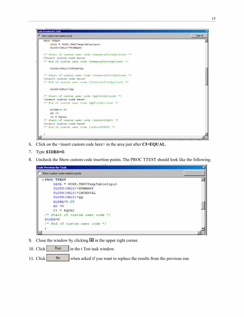
6. Click on the <insert custom code here> in the area just after CI=EQUAL.

7. Type SIDES=U.

8. Uncheck the Show custom code insertion points. The PROC TTEST should look like the following.

9. Close the window by clicking in the upper right corner.

10. Click in the t Test task window.

11. Click when asked if you want to replace the results from the previous run.

18

Notice that the confidence limits for the difference between Female and Male are different than in the

previous output, even though the Mean Diff is exactly the same.

The upper confidence bound for the difference is now Infty (Infinity). For left-sided tests, the lower

bound would be infinite in the negative direction.

The p-value for the difference between Female and Male (0.0321) is now significant at the 0.05 level.

The Confidence Interval Plot reflects the one-sided nature of the analysis. This time, the confidence

interval does not cross over zero.

The determination of whether to perform a one-sided test or two-sided test should be made before

any analysis or glancing at the data and should be made on subject-matter considerations and not

statistical power considerations.