sas studio 3 · 2016-02-16 · 9 chapter 3 / describe missing data ... ranking students by height...
TRANSCRIPT
SAS® Studio 3.5Task Reference
SAS® Documentation

The correct bibliographic citation for this manual is as follows: SAS Institute Inc. 2016. SAS® Studio 3.5: Task Reference Guide. Cary, NC: SAS Institute Inc.
SAS® Studio 3.5: Task Reference Guide
Copyright © 2016, SAS Institute Inc., Cary, NC, USA
All rights reserved. Produced in the United States of America.
For a hard-copy book: No part of this publication may be reproduced, stored in a retrieval system, or transmitted, in any form or by any means, electronic, mechanical, photocopying, or otherwise, without the prior written permission of the publisher, SAS Institute Inc.
For a web download or e-book: Your use of this publication shall be governed by the terms established by the vendor at the time you acquire this publication.
The scanning, uploading, and distribution of this book via the Internet or any other means without the permission of the publisher is illegal and punishable by law. Please purchase only authorized electronic editions and do not participate in or encourage electronic piracy of copyrighted materials. Your support of others' rights is appreciated.
U.S. Government License Rights; Restricted Rights: The Software and its documentation is commercial computer software developed at private expense and is provided with RESTRICTED RIGHTS to the United States Government. Use, duplication or disclosure of the Software by the United States Government is subject to the license terms of this Agreement pursuant to, as applicable, FAR 12.212, DFAR 227.7202-1(a), DFAR 227.7202-3(a) and DFAR 227.7202-4 and, to the extent required under U.S. federal law, the minimum restricted rights as set out in FAR 52.227-19 (DEC 2007). If FAR 52.227-19 is applicable, this provision serves as notice under clause (c) thereof and no other notice is required to be affixed to the Software or documentation. The Government's rights in Software and documentation shall be only those set forth in this Agreement.
SAS Institute Inc., SAS Campus Drive, Cary, North Carolina 27513-2414.
February 2016
SAS® and all other SAS Institute Inc. product or service names are registered trademarks or trademarks of SAS Institute Inc. in the USA and other countries. ® indicates USA registration.
Other brand and product names are trademarks of their respective companies.
Contents
Using This Book . . . . . . . . . . . . . . . . . . . . . . . . . . . . . . . . . . . . . . . . . . . . . . . . . . . . . . . xv
PART 1 Data Tasks 1
Chapter 1 / List Table Attributes . . . . . . . . . . . . . . . . . . . . . . . . . . . . . . . . . . . . . . . . . . . . . . . . . . . . . . . . . . 3About the List Table Attributes Task . . . . . . . . . . . . . . . . . . . . . . . . . . . . . . . . . . . . . . 3Example: Table Attributes for the Sashelp.Pricedata Data Set . . . . . . . . . . . . . . . 3Selecting an Input Data Source . . . . . . . . . . . . . . . . . . . . . . . . . . . . . . . . . . . . . . . . . . 5Setting Options . . . . . . . . . . . . . . . . . . . . . . . . . . . . . . . . . . . . . . . . . . . . . . . . . . . . . . . . 5
Chapter 2 / Characterize Data Task . . . . . . . . . . . . . . . . . . . . . . . . . . . . . . . . . . . . . . . . . . . . . . . . . . . . . . . . 7About the Characterize Data Task . . . . . . . . . . . . . . . . . . . . . . . . . . . . . . . . . . . . . . . 7Example: Characterize Data Task . . . . . . . . . . . . . . . . . . . . . . . . . . . . . . . . . . . . . . . . 7Assigning Data to Roles . . . . . . . . . . . . . . . . . . . . . . . . . . . . . . . . . . . . . . . . . . . . . . . . 9Setting Options . . . . . . . . . . . . . . . . . . . . . . . . . . . . . . . . . . . . . . . . . . . . . . . . . . . . . . . . 9
Chapter 3 / Describe Missing Data . . . . . . . . . . . . . . . . . . . . . . . . . . . . . . . . . . . . . . . . . . . . . . . . . . . . . . . 11About the Describe Missing Data Task . . . . . . . . . . . . . . . . . . . . . . . . . . . . . . . . . . 11Example: Describing Missing Data for SASHELP.BASEBALL . . . . . . . . . . . . . . . 11Setting the Data Options . . . . . . . . . . . . . . . . . . . . . . . . . . . . . . . . . . . . . . . . . . . . . . 13
Chapter 4 / List Data . . . . . . . . . . . . . . . . . . . . . . . . . . . . . . . . . . . . . . . . . . . . . . . . . . . . . . . . . . . . . . . . . . . . 15About the List Data Task . . . . . . . . . . . . . . . . . . . . . . . . . . . . . . . . . . . . . . . . . . . . . . 15Example: Reports of Drive Train, MSRP, and Engine Size by Car Type . . . . . . 15Assigning Data to Roles . . . . . . . . . . . . . . . . . . . . . . . . . . . . . . . . . . . . . . . . . . . . . . . 17Setting Options . . . . . . . . . . . . . . . . . . . . . . . . . . . . . . . . . . . . . . . . . . . . . . . . . . . . . . 17
Chapter 5 / Transpose Data . . . . . . . . . . . . . . . . . . . . . . . . . . . . . . . . . . . . . . . . . . . . . . . . . . . . . . . . . . . . . 21About the Transpose Data Task . . . . . . . . . . . . . . . . . . . . . . . . . . . . . . . . . . . . . . . . 21Example: Transposing the Data in the CLASS Data Set . . . . . . . . . . . . . . . . . . . 21Assigning Data to Roles . . . . . . . . . . . . . . . . . . . . . . . . . . . . . . . . . . . . . . . . . . . . . . . 22Setting Options . . . . . . . . . . . . . . . . . . . . . . . . . . . . . . . . . . . . . . . . . . . . . . . . . . . . . . 23
Chapter 6 / Stack/Split Columns . . . . . . . . . . . . . . . . . . . . . . . . . . . . . . . . . . . . . . . . . . . . . . . . . . . . . . . . . 25About the Stack/Split Columns Task . . . . . . . . . . . . . . . . . . . . . . . . . . . . . . . . . . . . 25Stacking Columns . . . . . . . . . . . . . . . . . . . . . . . . . . . . . . . . . . . . . . . . . . . . . . . . . . . . 26Splitting Columns . . . . . . . . . . . . . . . . . . . . . . . . . . . . . . . . . . . . . . . . . . . . . . . . . . . . . 30
Chapter 7 / Filter Data . . . . . . . . . . . . . . . . . . . . . . . . . . . . . . . . . . . . . . . . . . . . . . . . . . . . . . . . . . . . . . . . . . 37About the Filter Data Task . . . . . . . . . . . . . . . . . . . . . . . . . . . . . . . . . . . . . . . . . . . . . 37Example 1: Creating a Simple Filter . . . . . . . . . . . . . . . . . . . . . . . . . . . . . . . . . . . . . 37Example 2: Creating a Compound Filter . . . . . . . . . . . . . . . . . . . . . . . . . . . . . . . . . 38Creating Your Filter . . . . . . . . . . . . . . . . . . . . . . . . . . . . . . . . . . . . . . . . . . . . . . . . . . . 39
Chapter 8 / Select Random Sample . . . . . . . . . . . . . . . . . . . . . . . . . . . . . . . . . . . . . . . . . . . . . . . . . . . . . . . 41About the Select Random Sample Task . . . . . . . . . . . . . . . . . . . . . . . . . . . . . . . . . 41Example: Creating a Random Sample of the Sashelp.Pricedata Data Set . . . . 41Assigning Data to Roles . . . . . . . . . . . . . . . . . . . . . . . . . . . . . . . . . . . . . . . . . . . . . . . 43Setting Options . . . . . . . . . . . . . . . . . . . . . . . . . . . . . . . . . . . . . . . . . . . . . . . . . . . . . . 45
Chapter 9 / Partition Data . . . . . . . . . . . . . . . . . . . . . . . . . . . . . . . . . . . . . . . . . . . . . . . . . . . . . . . . . . . . . . . 47About the Partition Data Task . . . . . . . . . . . . . . . . . . . . . . . . . . . . . . . . . . . . . . . . . . 47Example: Partitioning the SASHELP.CLASSFIT Data Set . . . . . . . . . . . . . . . . . . 47Creating a Partitioned Data Set . . . . . . . . . . . . . . . . . . . . . . . . . . . . . . . . . . . . . . . . 48
Chapter 10 / Sort Data . . . . . . . . . . . . . . . . . . . . . . . . . . . . . . . . . . . . . . . . . . . . . . . . . . . . . . . . . . . . . . . . . . 51About the Sort Data Task . . . . . . . . . . . . . . . . . . . . . . . . . . . . . . . . . . . . . . . . . . . . . . 51Example: Sort the SASHELP.CLASS Data Set by Sex and Age . . . . . . . . . . . . . 51Assigning Data to Roles . . . . . . . . . . . . . . . . . . . . . . . . . . . . . . . . . . . . . . . . . . . . . . . 52Setting Options . . . . . . . . . . . . . . . . . . . . . . . . . . . . . . . . . . . . . . . . . . . . . . . . . . . . . . 53
Chapter 11 / Rank Data . . . . . . . . . . . . . . . . . . . . . . . . . . . . . . . . . . . . . . . . . . . . . . . . . . . . . . . . . . . . . . . . . 55About the Rank Data Task . . . . . . . . . . . . . . . . . . . . . . . . . . . . . . . . . . . . . . . . . . . . . 55Example: Ranking Students by Height within Age . . . . . . . . . . . . . . . . . . . . . . . . . 55Assigning Data to Roles . . . . . . . . . . . . . . . . . . . . . . . . . . . . . . . . . . . . . . . . . . . . . . . 56Setting Options . . . . . . . . . . . . . . . . . . . . . . . . . . . . . . . . . . . . . . . . . . . . . . . . . . . . . . 57
Chapter 12 / Transform Data . . . . . . . . . . . . . . . . . . . . . . . . . . . . . . . . . . . . . . . . . . . . . . . . . . . . . . . . . . . . 61About the Transform Data Task . . . . . . . . . . . . . . . . . . . . . . . . . . . . . . . . . . . . . . . . . 61Example: Transforming the Data in the BASEBALL Data Set . . . . . . . . . . . . . . . 61Transforming Columns from the Input Data Set . . . . . . . . . . . . . . . . . . . . . . . . . . . 63
Chapter 13 / Standardize Data . . . . . . . . . . . . . . . . . . . . . . . . . . . . . . . . . . . . . . . . . . . . . . . . . . . . . . . . . . . 65About the Standardize Data Task . . . . . . . . . . . . . . . . . . . . . . . . . . . . . . . . . . . . . . . 65Example: Standardizing Variables in the SASHELP.BASEBALL Data Set . . . . 65Assigning Data to Roles . . . . . . . . . . . . . . . . . . . . . . . . . . . . . . . . . . . . . . . . . . . . . . . 66Setting the Options . . . . . . . . . . . . . . . . . . . . . . . . . . . . . . . . . . . . . . . . . . . . . . . . . . . 67Setting the Output Options . . . . . . . . . . . . . . . . . . . . . . . . . . . . . . . . . . . . . . . . . . . . . 68
PART 2 Graph Tasks 69
Chapter 14 / Bar Chart . . . . . . . . . . . . . . . . . . . . . . . . . . . . . . . . . . . . . . . . . . . . . . . . . . . . . . . . . . . . . . . . . . 71About the Bar Chart Task . . . . . . . . . . . . . . . . . . . . . . . . . . . . . . . . . . . . . . . . . . . . . . 71Example: Bar Chart of Mean Sales for Each Product Line . . . . . . . . . . . . . . . . . . 71Assigning Data to Roles . . . . . . . . . . . . . . . . . . . . . . . . . . . . . . . . . . . . . . . . . . . . . . . 72Setting Options . . . . . . . . . . . . . . . . . . . . . . . . . . . . . . . . . . . . . . . . . . . . . . . . . . . . . . 74
Chapter 15 / Bar-Line Chart . . . . . . . . . . . . . . . . . . . . . . . . . . . . . . . . . . . . . . . . . . . . . . . . . . . . . . . . . . . . . 77About the Bar-Line Chart Task . . . . . . . . . . . . . . . . . . . . . . . . . . . . . . . . . . . . . . . . . 77Example: City and Highway Mileage by Origin . . . . . . . . . . . . . . . . . . . . . . . . . . . . 77Assigning Data to Roles . . . . . . . . . . . . . . . . . . . . . . . . . . . . . . . . . . . . . . . . . . . . . . . 78Setting Options . . . . . . . . . . . . . . . . . . . . . . . . . . . . . . . . . . . . . . . . . . . . . . . . . . . . . . 79
Chapter 16 / Box Plot . . . . . . . . . . . . . . . . . . . . . . . . . . . . . . . . . . . . . . . . . . . . . . . . . . . . . . . . . . . . . . . . . . . 83About the Box Plot Task . . . . . . . . . . . . . . . . . . . . . . . . . . . . . . . . . . . . . . . . . . . . . . . 83Example: Box Plots Comparing MPG (City) for Cars . . . . . . . . . . . . . . . . . . . . . . 83Assigning Data to Roles . . . . . . . . . . . . . . . . . . . . . . . . . . . . . . . . . . . . . . . . . . . . . . . 84
iv Contents
Setting Options . . . . . . . . . . . . . . . . . . . . . . . . . . . . . . . . . . . . . . . . . . . . . . . . . . . . . . 85
Chapter 17 / Bubble Plot . . . . . . . . . . . . . . . . . . . . . . . . . . . . . . . . . . . . . . . . . . . . . . . . . . . . . . . . . . . . . . . . 87About the Bubble Plot Task . . . . . . . . . . . . . . . . . . . . . . . . . . . . . . . . . . . . . . . . . . . . 87Example: Bubble Plot . . . . . . . . . . . . . . . . . . . . . . . . . . . . . . . . . . . . . . . . . . . . . . . . . 87Assigning Data to Roles . . . . . . . . . . . . . . . . . . . . . . . . . . . . . . . . . . . . . . . . . . . . . . . 88Setting Options . . . . . . . . . . . . . . . . . . . . . . . . . . . . . . . . . . . . . . . . . . . . . . . . . . . . . . 89
Chapter 18 / Histogram . . . . . . . . . . . . . . . . . . . . . . . . . . . . . . . . . . . . . . . . . . . . . . . . . . . . . . . . . . . . . . . . . 91About the Histogram Task . . . . . . . . . . . . . . . . . . . . . . . . . . . . . . . . . . . . . . . . . . . . . 91Example: Histogram of Stock Volume . . . . . . . . . . . . . . . . . . . . . . . . . . . . . . . . . . . 91Assigning Data to Roles . . . . . . . . . . . . . . . . . . . . . . . . . . . . . . . . . . . . . . . . . . . . . . . 92Setting Options . . . . . . . . . . . . . . . . . . . . . . . . . . . . . . . . . . . . . . . . . . . . . . . . . . . . . . 92
Chapter 19 / Line Chart . . . . . . . . . . . . . . . . . . . . . . . . . . . . . . . . . . . . . . . . . . . . . . . . . . . . . . . . . . . . . . . . . 95About the Line Chart Task . . . . . . . . . . . . . . . . . . . . . . . . . . . . . . . . . . . . . . . . . . . . . 95Example: Displaying the Mean Horsepower for Each Car Type . . . . . . . . . . . . . 95Assigning Data to Roles . . . . . . . . . . . . . . . . . . . . . . . . . . . . . . . . . . . . . . . . . . . . . . . 96Setting Options . . . . . . . . . . . . . . . . . . . . . . . . . . . . . . . . . . . . . . . . . . . . . . . . . . . . . . 97
Chapter 20 / Mosaic Plot . . . . . . . . . . . . . . . . . . . . . . . . . . . . . . . . . . . . . . . . . . . . . . . . . . . . . . . . . . . . . . . . 99About the Mosaic Plot Task . . . . . . . . . . . . . . . . . . . . . . . . . . . . . . . . . . . . . . . . . . . . 99Example: Mosaic Plot . . . . . . . . . . . . . . . . . . . . . . . . . . . . . . . . . . . . . . . . . . . . . . . . . 99Assigning Data to Roles . . . . . . . . . . . . . . . . . . . . . . . . . . . . . . . . . . . . . . . . . . . . . . 100Setting Options . . . . . . . . . . . . . . . . . . . . . . . . . . . . . . . . . . . . . . . . . . . . . . . . . . . . . 101
Chapter 21 / Pie Chart . . . . . . . . . . . . . . . . . . . . . . . . . . . . . . . . . . . . . . . . . . . . . . . . . . . . . . . . . . . . . . . . . 103About the Pie Chart Task . . . . . . . . . . . . . . . . . . . . . . . . . . . . . . . . . . . . . . . . . . . . . 103Example: Pie Chart That Shows Total MSRP for Each Car Type by Region . 103Assigning Data to Roles . . . . . . . . . . . . . . . . . . . . . . . . . . . . . . . . . . . . . . . . . . . . . . 104Setting Options . . . . . . . . . . . . . . . . . . . . . . . . . . . . . . . . . . . . . . . . . . . . . . . . . . . . . 105
Chapter 22 / Scatter Plot . . . . . . . . . . . . . . . . . . . . . . . . . . . . . . . . . . . . . . . . . . . . . . . . . . . . . . . . . . . . . . . 107About the Scatter Plot Task . . . . . . . . . . . . . . . . . . . . . . . . . . . . . . . . . . . . . . . . . . . 107Example: Scatter Plot of Height versus Weight . . . . . . . . . . . . . . . . . . . . . . . . . . 107Assigning Data to Roles . . . . . . . . . . . . . . . . . . . . . . . . . . . . . . . . . . . . . . . . . . . . . . 108Setting Options . . . . . . . . . . . . . . . . . . . . . . . . . . . . . . . . . . . . . . . . . . . . . . . . . . . . . 110
Chapter 23 / Series Plot . . . . . . . . . . . . . . . . . . . . . . . . . . . . . . . . . . . . . . . . . . . . . . . . . . . . . . . . . . . . . . . . 111About the Series Plot Task . . . . . . . . . . . . . . . . . . . . . . . . . . . . . . . . . . . . . . . . . . . . 111Example: Series Plot of Stock Trends . . . . . . . . . . . . . . . . . . . . . . . . . . . . . . . . . . 111Assigning Data to Roles . . . . . . . . . . . . . . . . . . . . . . . . . . . . . . . . . . . . . . . . . . . . . . 112Setting Options . . . . . . . . . . . . . . . . . . . . . . . . . . . . . . . . . . . . . . . . . . . . . . . . . . . . . 113
Chapter 24 / Simple HBar . . . . . . . . . . . . . . . . . . . . . . . . . . . . . . . . . . . . . . . . . . . . . . . . . . . . . . . . . . . . . . 115About the Simple HBar Task . . . . . . . . . . . . . . . . . . . . . . . . . . . . . . . . . . . . . . . . . . 115Example: Horizontal Bar Chart of Mileage by Origin and Type . . . . . . . . . . . . . 115Assigning Data to Roles . . . . . . . . . . . . . . . . . . . . . . . . . . . . . . . . . . . . . . . . . . . . . . 116Setting Options . . . . . . . . . . . . . . . . . . . . . . . . . . . . . . . . . . . . . . . . . . . . . . . . . . . . . 117
Contents v

PART 3 Combinatorics and Probability Tasks 121
Chapter 25 / Permutations . . . . . . . . . . . . . . . . . . . . . . . . . . . . . . . . . . . . . . . . . . . . . . . . . . . . . . . . . . . . . 123About the Permutations Task . . . . . . . . . . . . . . . . . . . . . . . . . . . . . . . . . . . . . . . . . 123Example: Calculating the Permutations of Six Objects . . . . . . . . . . . . . . . . . . . . 123Setting Options . . . . . . . . . . . . . . . . . . . . . . . . . . . . . . . . . . . . . . . . . . . . . . . . . . . . . 124
Chapter 26 / Combinations . . . . . . . . . . . . . . . . . . . . . . . . . . . . . . . . . . . . . . . . . . . . . . . . . . . . . . . . . . . . . 125About the Combinations Task . . . . . . . . . . . . . . . . . . . . . . . . . . . . . . . . . . . . . . . . . 125Example: Calculating the Combinations of 52 Objects in 5 Sets . . . . . . . . . . . 125Setting Options . . . . . . . . . . . . . . . . . . . . . . . . . . . . . . . . . . . . . . . . . . . . . . . . . . . . . 126
Chapter 27 / Same Birthday Probability . . . . . . . . . . . . . . . . . . . . . . . . . . . . . . . . . . . . . . . . . . . . . . . . . . 127About the Same Birthday Probability Task . . . . . . . . . . . . . . . . . . . . . . . . . . . . . . 127Example: Probability of Two or More People Sharing a
Birthday in a Room of 145 People . . . . . . . . . . . . . . . . . . . . . . . . . . . . . . . . . . 127Setting Options . . . . . . . . . . . . . . . . . . . . . . . . . . . . . . . . . . . . . . . . . . . . . . . . . . . . . 128
Chapter 28 / Dice Roll Simulation . . . . . . . . . . . . . . . . . . . . . . . . . . . . . . . . . . . . . . . . . . . . . . . . . . . . . . . 129About the Dice Roll Simulation Task . . . . . . . . . . . . . . . . . . . . . . . . . . . . . . . . . . . 129Example: Probability of Outcomes for 100,000,000 Dice Rolls . . . . . . . . . . . . . 129Setting Options . . . . . . . . . . . . . . . . . . . . . . . . . . . . . . . . . . . . . . . . . . . . . . . . . . . . . 130
Chapter 29 / Coin Toss Simulation . . . . . . . . . . . . . . . . . . . . . . . . . . . . . . . . . . . . . . . . . . . . . . . . . . . . . . 131About the Coin Toss Simulation Task . . . . . . . . . . . . . . . . . . . . . . . . . . . . . . . . . . . 131Example: Probability of Outcomes for 10,000,000 Coin Tosses . . . . . . . . . . . . 131Setting Options . . . . . . . . . . . . . . . . . . . . . . . . . . . . . . . . . . . . . . . . . . . . . . . . . . . . . 132
Chapter 30 / Poker Hand Probability . . . . . . . . . . . . . . . . . . . . . . . . . . . . . . . . . . . . . . . . . . . . . . . . . . . . 133About the Poker Hand Probability Task . . . . . . . . . . . . . . . . . . . . . . . . . . . . . . . . . 133Example: Results from the Poker Hand Probability Task . . . . . . . . . . . . . . . . . . 133
PART 4 Statistics Tasks 135
Chapter 31 / Data Exploration . . . . . . . . . . . . . . . . . . . . . . . . . . . . . . . . . . . . . . . . . . . . . . . . . . . . . . . . . . 137About the Data Exploration Task . . . . . . . . . . . . . . . . . . . . . . . . . . . . . . . . . . . . . . 137Example: Exploring the SASHELP.CARS Data . . . . . . . . . . . . . . . . . . . . . . . . . . 137Assigning Data to Roles . . . . . . . . . . . . . . . . . . . . . . . . . . . . . . . . . . . . . . . . . . . . . . 139Setting the Plot Options . . . . . . . . . . . . . . . . . . . . . . . . . . . . . . . . . . . . . . . . . . . . . . 139
Chapter 32 / Summary Statistics . . . . . . . . . . . . . . . . . . . . . . . . . . . . . . . . . . . . . . . . . . . . . . . . . . . . . . . . 143About the Summary Statistics Task . . . . . . . . . . . . . . . . . . . . . . . . . . . . . . . . . . . . 143Example: Summary Statistics of Unit Sales . . . . . . . . . . . . . . . . . . . . . . . . . . . . . 143Assigning Data to Roles . . . . . . . . . . . . . . . . . . . . . . . . . . . . . . . . . . . . . . . . . . . . . . 144Setting Options . . . . . . . . . . . . . . . . . . . . . . . . . . . . . . . . . . . . . . . . . . . . . . . . . . . . . 145Setting the Output Options . . . . . . . . . . . . . . . . . . . . . . . . . . . . . . . . . . . . . . . . . . . 149
Chapter 33 / Distribution Analysis . . . . . . . . . . . . . . . . . . . . . . . . . . . . . . . . . . . . . . . . . . . . . . . . . . . . . . 151About the Distribution Analysis Task . . . . . . . . . . . . . . . . . . . . . . . . . . . . . . . . . . . 151Example: Distribution Analysis of Sales for Each Region . . . . . . . . . . . . . . . . . 151Assigning Data to Roles . . . . . . . . . . . . . . . . . . . . . . . . . . . . . . . . . . . . . . . . . . . . . . 153
vi Contents
Setting Options . . . . . . . . . . . . . . . . . . . . . . . . . . . . . . . . . . . . . . . . . . . . . . . . . . . . . 154
Chapter 34 / One-Way Frequencies . . . . . . . . . . . . . . . . . . . . . . . . . . . . . . . . . . . . . . . . . . . . . . . . . . . . . 157About the One-Way Frequencies Task . . . . . . . . . . . . . . . . . . . . . . . . . . . . . . . . . 157Example: One-Way Frequencies of Unit Sales . . . . . . . . . . . . . . . . . . . . . . . . . . 157Assigning Data to Roles . . . . . . . . . . . . . . . . . . . . . . . . . . . . . . . . . . . . . . . . . . . . . . 159Setting Options . . . . . . . . . . . . . . . . . . . . . . . . . . . . . . . . . . . . . . . . . . . . . . . . . . . . . 160
Chapter 35 / Correlation Analysis . . . . . . . . . . . . . . . . . . . . . . . . . . . . . . . . . . . . . . . . . . . . . . . . . . . . . . . 163About the Correlation Analysis Task . . . . . . . . . . . . . . . . . . . . . . . . . . . . . . . . . . . 163Example: Correlations in the Sashelp.Cars Data Set . . . . . . . . . . . . . . . . . . . . . 163Assigning Data to Roles . . . . . . . . . . . . . . . . . . . . . . . . . . . . . . . . . . . . . . . . . . . . . . 164Setting Options . . . . . . . . . . . . . . . . . . . . . . . . . . . . . . . . . . . . . . . . . . . . . . . . . . . . . 165Setting the Output Options . . . . . . . . . . . . . . . . . . . . . . . . . . . . . . . . . . . . . . . . . . . 167
Chapter 36 / Table Analysis . . . . . . . . . . . . . . . . . . . . . . . . . . . . . . . . . . . . . . . . . . . . . . . . . . . . . . . . . . . . 169About the Table Analysis Task . . . . . . . . . . . . . . . . . . . . . . . . . . . . . . . . . . . . . . . . 169Example: Distribution of Type by DriveTrain . . . . . . . . . . . . . . . . . . . . . . . . . . . . . 169Assigning Data to Roles . . . . . . . . . . . . . . . . . . . . . . . . . . . . . . . . . . . . . . . . . . . . . . 171Setting Options . . . . . . . . . . . . . . . . . . . . . . . . . . . . . . . . . . . . . . . . . . . . . . . . . . . . . 171
Chapter 37 / t Tests . . . . . . . . . . . . . . . . . . . . . . . . . . . . . . . . . . . . . . . . . . . . . . . . . . . . . . . . . . . . . . . . . . . 175About the t Tests Task . . . . . . . . . . . . . . . . . . . . . . . . . . . . . . . . . . . . . . . . . . . . . . . 175One-Sample t Test . . . . . . . . . . . . . . . . . . . . . . . . . . . . . . . . . . . . . . . . . . . . . . . . . . 176Paired Test . . . . . . . . . . . . . . . . . . . . . . . . . . . . . . . . . . . . . . . . . . . . . . . . . . . . . . . . . 180Two-Sample t Test . . . . . . . . . . . . . . . . . . . . . . . . . . . . . . . . . . . . . . . . . . . . . . . . . . . 184
Chapter 38 / One-Way ANOVA . . . . . . . . . . . . . . . . . . . . . . . . . . . . . . . . . . . . . . . . . . . . . . . . . . . . . . . . . . 191About the One-Way ANOVA Task . . . . . . . . . . . . . . . . . . . . . . . . . . . . . . . . . . . . . 191Example: Testing for Differences in the Means for
MPG_Highway by Car Type . . . . . . . . . . . . . . . . . . . . . . . . . . . . . . . . . . . . . . . 191Assigning Data to Roles . . . . . . . . . . . . . . . . . . . . . . . . . . . . . . . . . . . . . . . . . . . . . . 194Setting Options . . . . . . . . . . . . . . . . . . . . . . . . . . . . . . . . . . . . . . . . . . . . . . . . . . . . . 195Setting the Output Options . . . . . . . . . . . . . . . . . . . . . . . . . . . . . . . . . . . . . . . . . . . 197
Chapter 39 / Nonparametric One-Way ANOVA . . . . . . . . . . . . . . . . . . . . . . . . . . . . . . . . . . . . . . . . . . . . 199About the Nonparametric One-Way ANOVA Task . . . . . . . . . . . . . . . . . . . . . . . . 199Example: Wilcoxon Scores for MPG_Highway Classified by Origin . . . . . . . . . 199Assigning Data to Roles . . . . . . . . . . . . . . . . . . . . . . . . . . . . . . . . . . . . . . . . . . . . . . 201Setting Options . . . . . . . . . . . . . . . . . . . . . . . . . . . . . . . . . . . . . . . . . . . . . . . . . . . . . 202Creating an Output Data Set . . . . . . . . . . . . . . . . . . . . . . . . . . . . . . . . . . . . . . . . . . 204
Chapter 40 / N-Way ANOVA . . . . . . . . . . . . . . . . . . . . . . . . . . . . . . . . . . . . . . . . . . . . . . . . . . . . . . . . . . . . 205About the N-Way ANOVA Task . . . . . . . . . . . . . . . . . . . . . . . . . . . . . . . . . . . . . . . . 205Example: Analyzing the Sashelp.RevHub2 Data Set . . . . . . . . . . . . . . . . . . . . . 205Assigning Data to Roles . . . . . . . . . . . . . . . . . . . . . . . . . . . . . . . . . . . . . . . . . . . . . . 207Building a Model . . . . . . . . . . . . . . . . . . . . . . . . . . . . . . . . . . . . . . . . . . . . . . . . . . . . 207Setting Options . . . . . . . . . . . . . . . . . . . . . . . . . . . . . . . . . . . . . . . . . . . . . . . . . . . . . 209Setting the Output Options . . . . . . . . . . . . . . . . . . . . . . . . . . . . . . . . . . . . . . . . . . . 209
Chapter 41 / Analysis of Covariance . . . . . . . . . . . . . . . . . . . . . . . . . . . . . . . . . . . . . . . . . . . . . . . . . . . . . 211About the Analysis of Covariance Task . . . . . . . . . . . . . . . . . . . . . . . . . . . . . . . . . 211Example: Analyzing the Sashelp.Class Data Set . . . . . . . . . . . . . . . . . . . . . . . . . 211Assigning Data to Roles . . . . . . . . . . . . . . . . . . . . . . . . . . . . . . . . . . . . . . . . . . . . . . 213Setting Options . . . . . . . . . . . . . . . . . . . . . . . . . . . . . . . . . . . . . . . . . . . . . . . . . . . . . 214Setting the Output Options . . . . . . . . . . . . . . . . . . . . . . . . . . . . . . . . . . . . . . . . . . . 215
Contents vii
Chapter 42 / Linear Regression . . . . . . . . . . . . . . . . . . . . . . . . . . . . . . . . . . . . . . . . . . . . . . . . . . . . . . . . . 217About the Linear Regression Task . . . . . . . . . . . . . . . . . . . . . . . . . . . . . . . . . . . . . 217Example: Predicting Weight Based on a Student’s Height . . . . . . . . . . . . . . . . . 217Assigning Data to Roles . . . . . . . . . . . . . . . . . . . . . . . . . . . . . . . . . . . . . . . . . . . . . . 220Building a Model . . . . . . . . . . . . . . . . . . . . . . . . . . . . . . . . . . . . . . . . . . . . . . . . . . . . 222Setting the Model Options . . . . . . . . . . . . . . . . . . . . . . . . . . . . . . . . . . . . . . . . . . . . 224Setting the Model Selection Options . . . . . . . . . . . . . . . . . . . . . . . . . . . . . . . . . . . 227Creating Output Data Sets . . . . . . . . . . . . . . . . . . . . . . . . . . . . . . . . . . . . . . . . . . . . 229
Chapter 43 / Binary Logistic Regression . . . . . . . . . . . . . . . . . . . . . . . . . . . . . . . . . . . . . . . . . . . . . . . . . 231About the Binary Logistic Regression Task . . . . . . . . . . . . . . . . . . . . . . . . . . . . . . 231Example: Classifying Email as Junk . . . . . . . . . . . . . . . . . . . . . . . . . . . . . . . . . . . 231Assigning Data to Roles . . . . . . . . . . . . . . . . . . . . . . . . . . . . . . . . . . . . . . . . . . . . . . 233Building a Model . . . . . . . . . . . . . . . . . . . . . . . . . . . . . . . . . . . . . . . . . . . . . . . . . . . . 235Specifying the Model Selection Options . . . . . . . . . . . . . . . . . . . . . . . . . . . . . . . . 237Setting Options . . . . . . . . . . . . . . . . . . . . . . . . . . . . . . . . . . . . . . . . . . . . . . . . . . . . . 239Creating Output Data Sets . . . . . . . . . . . . . . . . . . . . . . . . . . . . . . . . . . . . . . . . . . . . 242
Chapter 44 / Predictive Regression Models . . . . . . . . . . . . . . . . . . . . . . . . . . . . . . . . . . . . . . . . . . . . . . 245About the Predictive Regression Models Task . . . . . . . . . . . . . . . . . . . . . . . . . . . 245Example: Predicting a Baseball Player’s Salary . . . . . . . . . . . . . . . . . . . . . . . . . 246Partitioning Data . . . . . . . . . . . . . . . . . . . . . . . . . . . . . . . . . . . . . . . . . . . . . . . . . . . . 248Assigning Data to Roles . . . . . . . . . . . . . . . . . . . . . . . . . . . . . . . . . . . . . . . . . . . . . . 249Building a Model . . . . . . . . . . . . . . . . . . . . . . . . . . . . . . . . . . . . . . . . . . . . . . . . . . . . 250Selecting a Model . . . . . . . . . . . . . . . . . . . . . . . . . . . . . . . . . . . . . . . . . . . . . . . . . . . 253Setting the Options for the Final Model . . . . . . . . . . . . . . . . . . . . . . . . . . . . . . . . . 257Setting the Scoring Options . . . . . . . . . . . . . . . . . . . . . . . . . . . . . . . . . . . . . . . . . . . 258
Chapter 45 / Generalized Linear Models . . . . . . . . . . . . . . . . . . . . . . . . . . . . . . . . . . . . . . . . . . . . . . . . . 259About the Generalized Linear Models Task . . . . . . . . . . . . . . . . . . . . . . . . . . . . . 259Example: Analyzing the Sashelp.Baseball Data Set . . . . . . . . . . . . . . . . . . . . . . 260Assigning Data to Roles . . . . . . . . . . . . . . . . . . . . . . . . . . . . . . . . . . . . . . . . . . . . . . 261Building a Model . . . . . . . . . . . . . . . . . . . . . . . . . . . . . . . . . . . . . . . . . . . . . . . . . . . . 264Setting Options . . . . . . . . . . . . . . . . . . . . . . . . . . . . . . . . . . . . . . . . . . . . . . . . . . . . . 267Setting the Output Options . . . . . . . . . . . . . . . . . . . . . . . . . . . . . . . . . . . . . . . . . . . 269
Chapter 46 / Mixed Models . . . . . . . . . . . . . . . . . . . . . . . . . . . . . . . . . . . . . . . . . . . . . . . . . . . . . . . . . . . . . 271About the Mixed Models Task . . . . . . . . . . . . . . . . . . . . . . . . . . . . . . . . . . . . . . . . . 271Example: Analyzing Age and Gender . . . . . . . . . . . . . . . . . . . . . . . . . . . . . . . . . . 271Assigning Data to Roles . . . . . . . . . . . . . . . . . . . . . . . . . . . . . . . . . . . . . . . . . . . . . . 276Building a Model . . . . . . . . . . . . . . . . . . . . . . . . . . . . . . . . . . . . . . . . . . . . . . . . . . . . 277Setting the Options . . . . . . . . . . . . . . . . . . . . . . . . . . . . . . . . . . . . . . . . . . . . . . . . . . 281Creating Output Data Sets . . . . . . . . . . . . . . . . . . . . . . . . . . . . . . . . . . . . . . . . . . . . 282
Chapter 47 / Partial Least Squares Regression . . . . . . . . . . . . . . . . . . . . . . . . . . . . . . . . . . . . . . . . . . . 283About the Partial Least Squares Regression Task . . . . . . . . . . . . . . . . . . . . . . . 283Example: Partial Least Squares Regression Analysis . . . . . . . . . . . . . . . . . . . . 283Assigning Data to Roles . . . . . . . . . . . . . . . . . . . . . . . . . . . . . . . . . . . . . . . . . . . . . . 286Building a Model . . . . . . . . . . . . . . . . . . . . . . . . . . . . . . . . . . . . . . . . . . . . . . . . . . . . 287Setting Options . . . . . . . . . . . . . . . . . . . . . . . . . . . . . . . . . . . . . . . . . . . . . . . . . . . . . 290Creating Output Data Sets . . . . . . . . . . . . . . . . . . . . . . . . . . . . . . . . . . . . . . . . . . . . 292
viii Contents
PART 5 High-Performance Statistics Tasks 293
Chapter 48 / Bin Continuous Data . . . . . . . . . . . . . . . . . . . . . . . . . . . . . . . . . . . . . . . . . . . . . . . . . . . . . . . 295About the Bin Continuous Data Task . . . . . . . . . . . . . . . . . . . . . . . . . . . . . . . . . . . 295Example: Winsorized Binning . . . . . . . . . . . . . . . . . . . . . . . . . . . . . . . . . . . . . . . . . 295Assigning Data to Roles . . . . . . . . . . . . . . . . . . . . . . . . . . . . . . . . . . . . . . . . . . . . . . 297Setting Options . . . . . . . . . . . . . . . . . . . . . . . . . . . . . . . . . . . . . . . . . . . . . . . . . . . . . 298Creating an Output Data Set . . . . . . . . . . . . . . . . . . . . . . . . . . . . . . . . . . . . . . . . . . 299
Chapter 49 / High-Performance Correlation Analysis . . . . . . . . . . . . . . . . . . . . . . . . . . . . . . . . . . . . . . 301About the High-Performance Correlation Analysis Task . . . . . . . . . . . . . . . . . . . 301Example: Correlation between Weight, Oxygen, and Run Time . . . . . . . . . . . . 301Assigning Data to Roles . . . . . . . . . . . . . . . . . . . . . . . . . . . . . . . . . . . . . . . . . . . . . . 303Setting Options . . . . . . . . . . . . . . . . . . . . . . . . . . . . . . . . . . . . . . . . . . . . . . . . . . . . . 303Creating an Output Data Set . . . . . . . . . . . . . . . . . . . . . . . . . . . . . . . . . . . . . . . . . . 304
Chapter 50 / High-Performance Generalized Linear Models . . . . . . . . . . . . . . . . . . . . . . . . . . . . . . . . 305About the Generalized Linear Models Task . . . . . . . . . . . . . . . . . . . . . . . . . . . . . 305Example: Model Selection . . . . . . . . . . . . . . . . . . . . . . . . . . . . . . . . . . . . . . . . . . . . 305Partitioning Data . . . . . . . . . . . . . . . . . . . . . . . . . . . . . . . . . . . . . . . . . . . . . . . . . . . . 307Assigning Data to Roles . . . . . . . . . . . . . . . . . . . . . . . . . . . . . . . . . . . . . . . . . . . . . . 308Building a Model . . . . . . . . . . . . . . . . . . . . . . . . . . . . . . . . . . . . . . . . . . . . . . . . . . . . 311Setting the Model Selection Options . . . . . . . . . . . . . . . . . . . . . . . . . . . . . . . . . . . 314Setting Options . . . . . . . . . . . . . . . . . . . . . . . . . . . . . . . . . . . . . . . . . . . . . . . . . . . . . 316Setting the Output Options . . . . . . . . . . . . . . . . . . . . . . . . . . . . . . . . . . . . . . . . . . . 316
Chapter 51 / Replace Missing Values . . . . . . . . . . . . . . . . . . . . . . . . . . . . . . . . . . . . . . . . . . . . . . . . . . . . 317About the Replace Missing Values Task . . . . . . . . . . . . . . . . . . . . . . . . . . . . . . . . 317Assigning Data to Roles . . . . . . . . . . . . . . . . . . . . . . . . . . . . . . . . . . . . . . . . . . . . . . 317Setting the Output Options . . . . . . . . . . . . . . . . . . . . . . . . . . . . . . . . . . . . . . . . . . . 318
Chapter 52 / Random Sampling . . . . . . . . . . . . . . . . . . . . . . . . . . . . . . . . . . . . . . . . . . . . . . . . . . . . . . . . . 319About the Random Sampling Task . . . . . . . . . . . . . . . . . . . . . . . . . . . . . . . . . . . . . 319Assigning Data to Roles . . . . . . . . . . . . . . . . . . . . . . . . . . . . . . . . . . . . . . . . . . . . . . 319Creating the Output Data Set . . . . . . . . . . . . . . . . . . . . . . . . . . . . . . . . . . . . . . . . . 320Setting Options . . . . . . . . . . . . . . . . . . . . . . . . . . . . . . . . . . . . . . . . . . . . . . . . . . . . . 321
PART 6 Power and Sample Size 323
Chapter 53 / Pearson Correlation . . . . . . . . . . . . . . . . . . . . . . . . . . . . . . . . . . . . . . . . . . . . . . . . . . . . . . . 325About the Pearson Correlation Task . . . . . . . . . . . . . . . . . . . . . . . . . . . . . . . . . . . 325Example: Pearson Correlation for Power and Sample Size Analysis . . . . . . . . 325Assigning Properties . . . . . . . . . . . . . . . . . . . . . . . . . . . . . . . . . . . . . . . . . . . . . . . . . 326Setting the Plot Options . . . . . . . . . . . . . . . . . . . . . . . . . . . . . . . . . . . . . . . . . . . . . . 328
Chapter 54 / Multiple Regression . . . . . . . . . . . . . . . . . . . . . . . . . . . . . . . . . . . . . . . . . . . . . . . . . . . . . . . 329About the Multiple Regression Task . . . . . . . . . . . . . . . . . . . . . . . . . . . . . . . . . . . . 329Example: Solve for Power . . . . . . . . . . . . . . . . . . . . . . . . . . . . . . . . . . . . . . . . . . . . 329Assigning Properties . . . . . . . . . . . . . . . . . . . . . . . . . . . . . . . . . . . . . . . . . . . . . . . . . 331Setting the Plot Options . . . . . . . . . . . . . . . . . . . . . . . . . . . . . . . . . . . . . . . . . . . . . . 331
Contents ix
Chapter 55 / Confidence Intervals . . . . . . . . . . . . . . . . . . . . . . . . . . . . . . . . . . . . . . . . . . . . . . . . . . . . . . . 333About the Confidence Intervals Task . . . . . . . . . . . . . . . . . . . . . . . . . . . . . . . . . . . 333Example: Confidence Interval for One-Sample Means . . . . . . . . . . . . . . . . . . . . 333Assigning Properties . . . . . . . . . . . . . . . . . . . . . . . . . . . . . . . . . . . . . . . . . . . . . . . . . 334Setting the Plot Options . . . . . . . . . . . . . . . . . . . . . . . . . . . . . . . . . . . . . . . . . . . . . . 336
Chapter 56 / Tests of Proportions . . . . . . . . . . . . . . . . . . . . . . . . . . . . . . . . . . . . . . . . . . . . . . . . . . . . . . . 337About the Tests of Proportions Task . . . . . . . . . . . . . . . . . . . . . . . . . . . . . . . . . . . . 337Example: Power Analysis for One Proportion . . . . . . . . . . . . . . . . . . . . . . . . . . . 337Create a One-Proportion Test . . . . . . . . . . . . . . . . . . . . . . . . . . . . . . . . . . . . . . . . . 338Create a Two Correlated Proportions Test . . . . . . . . . . . . . . . . . . . . . . . . . . . . . . 339Create a Two Independent Proportions Test . . . . . . . . . . . . . . . . . . . . . . . . . . . . 339Setting the Plot Options . . . . . . . . . . . . . . . . . . . . . . . . . . . . . . . . . . . . . . . . . . . . . . 340
Chapter 57 / t Tests . . . . . . . . . . . . . . . . . . . . . . . . . . . . . . . . . . . . . . . . . . . . . . . . . . . . . . . . . . . . . . . . . . . 341About the t Tests Task . . . . . . . . . . . . . . . . . . . . . . . . . . . . . . . . . . . . . . . . . . . . . . . 341Example: One-Sample t Test for Mean . . . . . . . . . . . . . . . . . . . . . . . . . . . . . . . . . 341Assigning Properties . . . . . . . . . . . . . . . . . . . . . . . . . . . . . . . . . . . . . . . . . . . . . . . . . 342Setting the Plot Options . . . . . . . . . . . . . . . . . . . . . . . . . . . . . . . . . . . . . . . . . . . . . . 344
Chapter 58 / Cox Regression . . . . . . . . . . . . . . . . . . . . . . . . . . . . . . . . . . . . . . . . . . . . . . . . . . . . . . . . . . . 345About the Cox Regression Task . . . . . . . . . . . . . . . . . . . . . . . . . . . . . . . . . . . . . . . 345Example: Cox Regression . . . . . . . . . . . . . . . . . . . . . . . . . . . . . . . . . . . . . . . . . . . . 345Assigning Properties . . . . . . . . . . . . . . . . . . . . . . . . . . . . . . . . . . . . . . . . . . . . . . . . . 346Setting the Plot Options . . . . . . . . . . . . . . . . . . . . . . . . . . . . . . . . . . . . . . . . . . . . . . 347
PART 7 Multivariate Analysis 349
Chapter 59 / Principal Component Analysis . . . . . . . . . . . . . . . . . . . . . . . . . . . . . . . . . . . . . . . . . . . . . . 351About the Principal Component Analysis Task . . . . . . . . . . . . . . . . . . . . . . . . . . . 351Example: Principal Component Analysis of Sashelp.Class Data Set . . . . . . . . 351Assigning Data to Roles . . . . . . . . . . . . . . . . . . . . . . . . . . . . . . . . . . . . . . . . . . . . . . 353Setting Options . . . . . . . . . . . . . . . . . . . . . . . . . . . . . . . . . . . . . . . . . . . . . . . . . . . . . 353Setting the Output Options . . . . . . . . . . . . . . . . . . . . . . . . . . . . . . . . . . . . . . . . . . . 354
Chapter 60 / Factor Analysis . . . . . . . . . . . . . . . . . . . . . . . . . . . . . . . . . . . . . . . . . . . . . . . . . . . . . . . . . . . 355About the Factor Analysis Task . . . . . . . . . . . . . . . . . . . . . . . . . . . . . . . . . . . . . . . . 355Example: Factor Analysis . . . . . . . . . . . . . . . . . . . . . . . . . . . . . . . . . . . . . . . . . . . . 355Assigning Data to Roles . . . . . . . . . . . . . . . . . . . . . . . . . . . . . . . . . . . . . . . . . . . . . . 357Setting Options . . . . . . . . . . . . . . . . . . . . . . . . . . . . . . . . . . . . . . . . . . . . . . . . . . . . . 358Setting the Output Options . . . . . . . . . . . . . . . . . . . . . . . . . . . . . . . . . . . . . . . . . . . 361
Chapter 61 / Canonical Correlation . . . . . . . . . . . . . . . . . . . . . . . . . . . . . . . . . . . . . . . . . . . . . . . . . . . . . . 363About the Canonical Correlation Analysis Task . . . . . . . . . . . . . . . . . . . . . . . . . . 363Example: Canonical Correlation Analysis . . . . . . . . . . . . . . . . . . . . . . . . . . . . . . . 363Assigning Data to Roles . . . . . . . . . . . . . . . . . . . . . . . . . . . . . . . . . . . . . . . . . . . . . . 365Setting Options . . . . . . . . . . . . . . . . . . . . . . . . . . . . . . . . . . . . . . . . . . . . . . . . . . . . . 366Setting the Output Options . . . . . . . . . . . . . . . . . . . . . . . . . . . . . . . . . . . . . . . . . . . 367
Chapter 62 / Discriminant Analysis . . . . . . . . . . . . . . . . . . . . . . . . . . . . . . . . . . . . . . . . . . . . . . . . . . . . . . 369About the Discriminant Analysis Task . . . . . . . . . . . . . . . . . . . . . . . . . . . . . . . . . . 369Example: Discriminant Analysis on Crops Data . . . . . . . . . . . . . . . . . . . . . . . . . . 369Assigning Data to Roles . . . . . . . . . . . . . . . . . . . . . . . . . . . . . . . . . . . . . . . . . . . . . . 372
x Contents
Setting Options . . . . . . . . . . . . . . . . . . . . . . . . . . . . . . . . . . . . . . . . . . . . . . . . . . . . . 373Setting the Selection Options . . . . . . . . . . . . . . . . . . . . . . . . . . . . . . . . . . . . . . . . . 375Setting the Output Options . . . . . . . . . . . . . . . . . . . . . . . . . . . . . . . . . . . . . . . . . . . 376
Chapter 63 / Correspondence Analysis . . . . . . . . . . . . . . . . . . . . . . . . . . . . . . . . . . . . . . . . . . . . . . . . . . 377About the Correspondence Analysis Task . . . . . . . . . . . . . . . . . . . . . . . . . . . . . . 377Example: Correspondence Analysis . . . . . . . . . . . . . . . . . . . . . . . . . . . . . . . . . . . 377Assigning Data to Roles . . . . . . . . . . . . . . . . . . . . . . . . . . . . . . . . . . . . . . . . . . . . . . 379Setting Options . . . . . . . . . . . . . . . . . . . . . . . . . . . . . . . . . . . . . . . . . . . . . . . . . . . . . 383Setting the Output Options . . . . . . . . . . . . . . . . . . . . . . . . . . . . . . . . . . . . . . . . . . . 384
Chapter 64 / Multidimensional Preferences Analysis . . . . . . . . . . . . . . . . . . . . . . . . . . . . . . . . . . . . . . 385About the Multidimensional Preference Analysis Task . . . . . . . . . . . . . . . . . . . . 385Example: Multidimensional Preference Analysis . . . . . . . . . . . . . . . . . . . . . . . . . 385Assigning Data to Roles . . . . . . . . . . . . . . . . . . . . . . . . . . . . . . . . . . . . . . . . . . . . . . 387Setting Options . . . . . . . . . . . . . . . . . . . . . . . . . . . . . . . . . . . . . . . . . . . . . . . . . . . . . 389Setting the Output Options . . . . . . . . . . . . . . . . . . . . . . . . . . . . . . . . . . . . . . . . . . . 390
PART 8 Econometrics Tasks 391
Chapter 65 / Causal Models . . . . . . . . . . . . . . . . . . . . . . . . . . . . . . . . . . . . . . . . . . . . . . . . . . . . . . . . . . . . 393About the Causal Models Task . . . . . . . . . . . . . . . . . . . . . . . . . . . . . . . . . . . . . . . . 393Two-Stage Least Squares . . . . . . . . . . . . . . . . . . . . . . . . . . . . . . . . . . . . . . . . . . . . 393Heckman’s Two-Step Selection Method . . . . . . . . . . . . . . . . . . . . . . . . . . . . . . . . 397
Chapter 66 / Cross-sectional Data Models . . . . . . . . . . . . . . . . . . . . . . . . . . . . . . . . . . . . . . . . . . . . . . . 403About the Cross-Sectional Data Models Task . . . . . . . . . . . . . . . . . . . . . . . . . . . 404Linear Models . . . . . . . . . . . . . . . . . . . . . . . . . . . . . . . . . . . . . . . . . . . . . . . . . . . . . . 404Logit Model . . . . . . . . . . . . . . . . . . . . . . . . . . . . . . . . . . . . . . . . . . . . . . . . . . . . . . . . . 408Probit Model . . . . . . . . . . . . . . . . . . . . . . . . . . . . . . . . . . . . . . . . . . . . . . . . . . . . . . . . 412Poisson Models . . . . . . . . . . . . . . . . . . . . . . . . . . . . . . . . . . . . . . . . . . . . . . . . . . . . . 417Negative Binomial Models . . . . . . . . . . . . . . . . . . . . . . . . . . . . . . . . . . . . . . . . . . . . 422Censored Regression . . . . . . . . . . . . . . . . . . . . . . . . . . . . . . . . . . . . . . . . . . . . . . . . 426Truncated Regression . . . . . . . . . . . . . . . . . . . . . . . . . . . . . . . . . . . . . . . . . . . . . . . 431
Chapter 67 / Panel Data Models . . . . . . . . . . . . . . . . . . . . . . . . . . . . . . . . . . . . . . . . . . . . . . . . . . . . . . . . . 435About the Panel Data Models Task . . . . . . . . . . . . . . . . . . . . . . . . . . . . . . . . . . . . 436Linear Models . . . . . . . . . . . . . . . . . . . . . . . . . . . . . . . . . . . . . . . . . . . . . . . . . . . . . . 436Logit Model . . . . . . . . . . . . . . . . . . . . . . . . . . . . . . . . . . . . . . . . . . . . . . . . . . . . . . . . . 441Probit Model . . . . . . . . . . . . . . . . . . . . . . . . . . . . . . . . . . . . . . . . . . . . . . . . . . . . . . . . 445Poisson Models . . . . . . . . . . . . . . . . . . . . . . . . . . . . . . . . . . . . . . . . . . . . . . . . . . . . . 450Negative Binomial Models . . . . . . . . . . . . . . . . . . . . . . . . . . . . . . . . . . . . . . . . . . . . 455Censored Regression . . . . . . . . . . . . . . . . . . . . . . . . . . . . . . . . . . . . . . . . . . . . . . . . 459Truncated Regression . . . . . . . . . . . . . . . . . . . . . . . . . . . . . . . . . . . . . . . . . . . . . . . 463
Chapter 68 / Time Series Analysis . . . . . . . . . . . . . . . . . . . . . . . . . . . . . . . . . . . . . . . . . . . . . . . . . . . . . . 469About the Time Series Analysis Task . . . . . . . . . . . . . . . . . . . . . . . . . . . . . . . . . . . 469Time Series Analysis for One Dependent Variable . . . . . . . . . . . . . . . . . . . . . . . 469Time Series Analysis for Multiple Dependent Variables . . . . . . . . . . . . . . . . . . . 475
Contents xi
PART 9 Forecasting Tasks 481
Chapter 69 / Time Series Data Preparation . . . . . . . . . . . . . . . . . . . . . . . . . . . . . . . . . . . . . . . . . . . . . . . 483About the Time Series Data Preparation Task . . . . . . . . . . . . . . . . . . . . . . . . . . . 483Understanding SAS Time Intervals . . . . . . . . . . . . . . . . . . . . . . . . . . . . . . . . . . . . 483Example: Transforming the Data in the Sashelp.PriceData Data Set . . . . . . . 486Assigning Data to Roles . . . . . . . . . . . . . . . . . . . . . . . . . . . . . . . . . . . . . . . . . . . . . . 487Setting the Transformations Options . . . . . . . . . . . . . . . . . . . . . . . . . . . . . . . . . . . 489Creating the Output Data Set . . . . . . . . . . . . . . . . . . . . . . . . . . . . . . . . . . . . . . . . . 490
Chapter 70 / Time Series Data Exploration . . . . . . . . . . . . . . . . . . . . . . . . . . . . . . . . . . . . . . . . . . . . . . . 491About the Time Series Exploration Task . . . . . . . . . . . . . . . . . . . . . . . . . . . . . . . . 491Example: Exploring the Sashelp.PriceData Data Set . . . . . . . . . . . . . . . . . . . . . 491Assigning Data to Roles . . . . . . . . . . . . . . . . . . . . . . . . . . . . . . . . . . . . . . . . . . . . . . 495Setting the Analyses Options . . . . . . . . . . . . . . . . . . . . . . . . . . . . . . . . . . . . . . . . . 496
Chapter 71 / Modeling and Forecasting Task . . . . . . . . . . . . . . . . . . . . . . . . . . . . . . . . . . . . . . . . . . . . . 501About the Modeling and Forecasting Task . . . . . . . . . . . . . . . . . . . . . . . . . . . . . . 501Example: Creating a Random Walk Model for the
SASHELP.PRICEDATA Data Set . . . . . . . . . . . . . . . . . . . . . . . . . . . . . . . . . . . 501Assigning Data to Roles . . . . . . . . . . . . . . . . . . . . . . . . . . . . . . . . . . . . . . . . . . . . . . 503Setting the Model Options . . . . . . . . . . . . . . . . . . . . . . . . . . . . . . . . . . . . . . . . . . . . 504Setting the Forecasting Options . . . . . . . . . . . . . . . . . . . . . . . . . . . . . . . . . . . . . . . 509Setting the Output Options . . . . . . . . . . . . . . . . . . . . . . . . . . . . . . . . . . . . . . . . . . . 509
PART 10 Statistical Process Control 511
Chapter 72 / Control Charts . . . . . . . . . . . . . . . . . . . . . . . . . . . . . . . . . . . . . . . . . . . . . . . . . . . . . . . . . . . . 513About the Control Charts Task . . . . . . . . . . . . . . . . . . . . . . . . . . . . . . . . . . . . . . . . 513Example: Determine the Mean and Range for the Diameters of Wafers . . . . . 522Assigning Data to Roles . . . . . . . . . . . . . . . . . . . . . . . . . . . . . . . . . . . . . . . . . . . . . . 524Setting Options . . . . . . . . . . . . . . . . . . . . . . . . . . . . . . . . . . . . . . . . . . . . . . . . . . . . . 525Setting the Output Options . . . . . . . . . . . . . . . . . . . . . . . . . . . . . . . . . . . . . . . . . . . 526
Chapter 73 / Capability Analysis . . . . . . . . . . . . . . . . . . . . . . . . . . . . . . . . . . . . . . . . . . . . . . . . . . . . . . . . 527About the Capability Analysis Task . . . . . . . . . . . . . . . . . . . . . . . . . . . . . . . . . . . . 527Example: Analysis of Plating Thickness . . . . . . . . . . . . . . . . . . . . . . . . . . . . . . . . 528Assigning Data to Roles . . . . . . . . . . . . . . . . . . . . . . . . . . . . . . . . . . . . . . . . . . . . . . 530Setting Options . . . . . . . . . . . . . . . . . . . . . . . . . . . . . . . . . . . . . . . . . . . . . . . . . . . . . 531Setting the Output Options . . . . . . . . . . . . . . . . . . . . . . . . . . . . . . . . . . . . . . . . . . . 531
Chapter 74 / Pareto Analysis . . . . . . . . . . . . . . . . . . . . . . . . . . . . . . . . . . . . . . . . . . . . . . . . . . . . . . . . . . . 533About the Pareto Analysis Task . . . . . . . . . . . . . . . . . . . . . . . . . . . . . . . . . . . . . . . 533Example: Causes of Failure . . . . . . . . . . . . . . . . . . . . . . . . . . . . . . . . . . . . . . . . . . 533Assigning Data to Roles . . . . . . . . . . . . . . . . . . . . . . . . . . . . . . . . . . . . . . . . . . . . . . 535Setting Options . . . . . . . . . . . . . . . . . . . . . . . . . . . . . . . . . . . . . . . . . . . . . . . . . . . . . 536Setting the Output Options . . . . . . . . . . . . . . . . . . . . . . . . . . . . . . . . . . . . . . . . . . . 536
Chapter 75 / Analysis of Means . . . . . . . . . . . . . . . . . . . . . . . . . . . . . . . . . . . . . . . . . . . . . . . . . . . . . . . . . 537About the Analysis of Means Task . . . . . . . . . . . . . . . . . . . . . . . . . . . . . . . . . . . . . 537Example: Determine the Deviation of Label Positions . . . . . . . . . . . . . . . . . . . . 541
xii Contents
Assigning Data to Roles . . . . . . . . . . . . . . . . . . . . . . . . . . . . . . . . . . . . . . . . . . . . . . 543Setting Options . . . . . . . . . . . . . . . . . . . . . . . . . . . . . . . . . . . . . . . . . . . . . . . . . . . . . 544Setting the Output Options . . . . . . . . . . . . . . . . . . . . . . . . . . . . . . . . . . . . . . . . . . . 545
PART 11 Data Mining Tasks 547
Chapter 76 / Rapid Predictive Modeler . . . . . . . . . . . . . . . . . . . . . . . . . . . . . . . . . . . . . . . . . . . . . . . . . . . 549About the Rapid Predictive Modeler . . . . . . . . . . . . . . . . . . . . . . . . . . . . . . . . . . . . 549Assigning Data to Roles . . . . . . . . . . . . . . . . . . . . . . . . . . . . . . . . . . . . . . . . . . . . . . 553Setting the Model Options . . . . . . . . . . . . . . . . . . . . . . . . . . . . . . . . . . . . . . . . . . . . 555Setting the Report Options . . . . . . . . . . . . . . . . . . . . . . . . . . . . . . . . . . . . . . . . . . . 558Setting the Output Options . . . . . . . . . . . . . . . . . . . . . . . . . . . . . . . . . . . . . . . . . . . 559
PART 12 Appendixes 561
Appendix 1 / Input Data Sets for Task Examples . . . . . . . . . . . . . . . . . . . . . . . . . . . . . . . . . . . . . . . . . . 563About the Task Data Sets . . . . . . . . . . . . . . . . . . . . . . . . . . . . . . . . . . . . . . . . . . . . 563CIGAR Data Set . . . . . . . . . . . . . . . . . . . . . . . . . . . . . . . . . . . . . . . . . . . . . . . . . . . . 563FITNESS Data set . . . . . . . . . . . . . . . . . . . . . . . . . . . . . . . . . . . . . . . . . . . . . . . . . . . 588GETSTARTED Data Set . . . . . . . . . . . . . . . . . . . . . . . . . . . . . . . . . . . . . . . . . . . . . 589GREENE Data Set . . . . . . . . . . . . . . . . . . . . . . . . . . . . . . . . . . . . . . . . . . . . . . . . . . 591IN Data Set . . . . . . . . . . . . . . . . . . . . . . . . . . . . . . . . . . . . . . . . . . . . . . . . . . . . . . . . . 591LONG97DATA Data Set . . . . . . . . . . . . . . . . . . . . . . . . . . . . . . . . . . . . . . . . . . . . . . 592MROZ Data Set . . . . . . . . . . . . . . . . . . . . . . . . . . . . . . . . . . . . . . . . . . . . . . . . . . . . . 608
Appendix 2 / References . . . . . . . . . . . . . . . . . . . . . . . . . . . . . . . . . . . . . . . . . . . . . . . . . . . . . . . . . . . . . . . 623
Recommended Reading . . . . . . . . . . . . . . . . . . . . . . . . . . . . . . . . . . . . . . . . . . . . . 625
Contents xiii

xiv Contents
Using This Book
Audience
This book is a reference guide for anyone who uses SAS Studio tasks. In this document, you can find descriptions of each task and all of the options that are available for each task. When appropriate, the task documentation includes an example that you can walkthrough. This document should be used in conjunction with the SAS Studio: User's Guide.
For information about how to develop custom tasks for your site, see SAS Studio: Developer's Guide.
Requirements
To run these tasks, you must have access to SAS Studio 3.5. Some tasks require additional SAS software. For example, some tasks require that you license and install SAS/STAT. If you have this additional products licensed and installed at your site, these tasks are available from the user interface. If you do not have the required software, these tasks do no appear in the user interface. The About topic for each task lists any software that is required to run the task.
xv

xvi Using This Book
Part 1
Data Tasks
Chapter 1List Table Attributes . . . . . . . . . . . . . . . . . . . . . . . . . . . . . . . . . . . . . . . . . . . . . . . 3
Chapter 2Characterize Data Task . . . . . . . . . . . . . . . . . . . . . . . . . . . . . . . . . . . . . . . . . . . . . 7
Chapter 3Describe Missing Data . . . . . . . . . . . . . . . . . . . . . . . . . . . . . . . . . . . . . . . . . . . . 11
Chapter 4List Data . . . . . . . . . . . . . . . . . . . . . . . . . . . . . . . . . . . . . . . . . . . . . . . . . . . . . . . . . 15
Chapter 5Transpose Data . . . . . . . . . . . . . . . . . . . . . . . . . . . . . . . . . . . . . . . . . . . . . . . . . . 21
Chapter 6Stack/Split Columns . . . . . . . . . . . . . . . . . . . . . . . . . . . . . . . . . . . . . . . . . . . . . . 25
Chapter 7Filter Data . . . . . . . . . . . . . . . . . . . . . . . . . . . . . . . . . . . . . . . . . . . . . . . . . . . . . . . 37
Chapter 8Select Random Sample . . . . . . . . . . . . . . . . . . . . . . . . . . . . . . . . . . . . . . . . . . . . 41
Chapter 9Partition Data . . . . . . . . . . . . . . . . . . . . . . . . . . . . . . . . . . . . . . . . . . . . . . . . . . . . 47
1

Chapter 10Sort Data . . . . . . . . . . . . . . . . . . . . . . . . . . . . . . . . . . . . . . . . . . . . . . . . . . . . . . . . 51
Chapter 11Rank Data . . . . . . . . . . . . . . . . . . . . . . . . . . . . . . . . . . . . . . . . . . . . . . . . . . . . . . . 55
Chapter 12Transform Data . . . . . . . . . . . . . . . . . . . . . . . . . . . . . . . . . . . . . . . . . . . . . . . . . . . 61
Chapter 13Standardize Data . . . . . . . . . . . . . . . . . . . . . . . . . . . . . . . . . . . . . . . . . . . . . . . . . 65
2

1List Table Attributes
About the List Table Attributes Task . . . . . . . . . . . . . . . . . . . . . . . . . . . . . . . . . . . . . . . . . 3
Example: Table Attributes for the Sashelp.Pricedata Data Set . . . . . . . . . . . . . . . . 3
Selecting an Input Data Source . . . . . . . . . . . . . . . . . . . . . . . . . . . . . . . . . . . . . . . . . . . . . . 5
Setting Options . . . . . . . . . . . . . . . . . . . . . . . . . . . . . . . . . . . . . . . . . . . . . . . . . . . . . . . . . . . . . . 5
About the List Table Attributes Task
The List Table Attributes task enables you to quickly see the date on which the data set was created and last modified, the number of rows, the encoding, any engine-dependent or host-dependent information, and an alphabetic list of the variables and their attributes. You can also view any directory and host/engine information by using this task.
Example: Table Attributes for the Sashelp.Pricedata Data Set
In this example, you want to view the table attributes for the Sashelp.Pricedata data set.
To create this example:
1 In the Tasks section, expand the Data folder, and then double-click List Table Attributes. The user interface for the List Table Attributes task opens.
2 On the Data tab, select the SASHELP.PRICEDATA data set.
TIP If the data set is not available from the drop-down list, click . In
the Choose a Table window, expand the library that contains the data set that you want to use. Select the data set for the example and click OK. The selected data set should now appear in the drop-down list.
3 On the Options tab, select Create output data set.
4 To run the task, click .
3
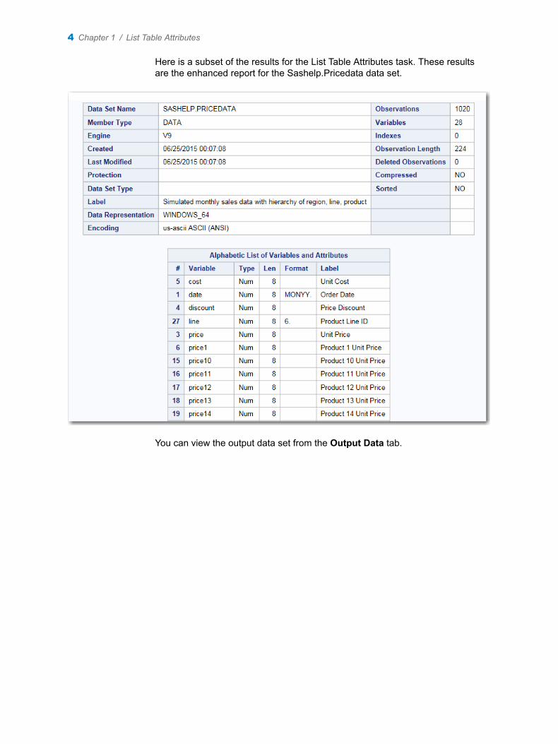
Here is a subset of the results for the List Table Attributes task. These results are the enhanced report for the Sashelp.Pricedata data set.
You can view the output data set from the Output Data tab.
4 Chapter 1 / List Table Attributes
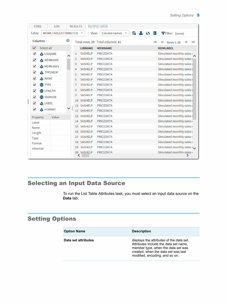
Selecting an Input Data Source
To run the List Table Attributes task, you must select an input data source on the Data tab.
Setting Options
Option Name Description
Data set attributes displays the attributes of the data set. Attributes include the data set name, member type, when the data set was created, when the data set was last modified, encoding, and so on.
Setting Options 5
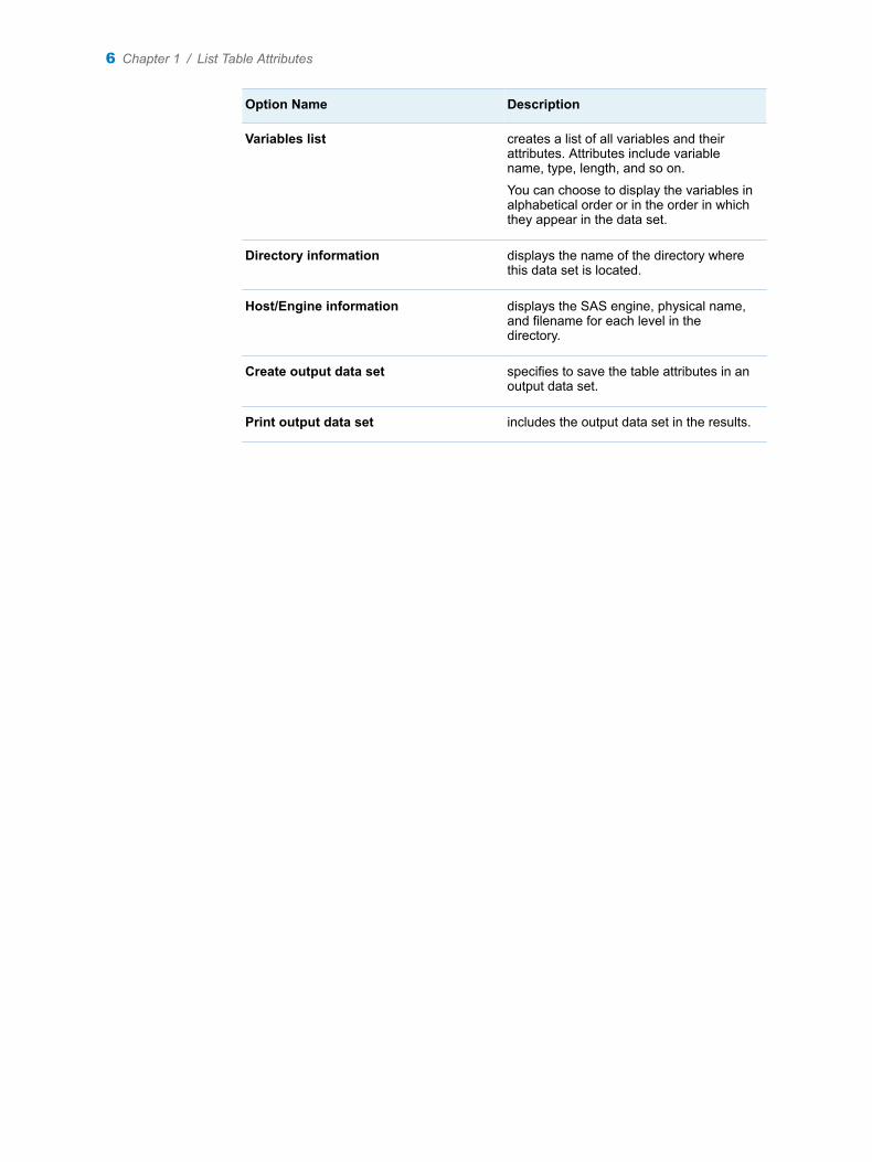
Option Name Description
Variables list creates a list of all variables and their attributes. Attributes include variable name, type, length, and so on.
You can choose to display the variables in alphabetical order or in the order in which they appear in the data set.
Directory information displays the name of the directory where this data set is located.
Host/Engine information displays the SAS engine, physical name, and filename for each level in the directory.
Create output data set specifies to save the table attributes in an output data set.
Print output data set includes the output data set in the results.
6 Chapter 1 / List Table Attributes
2Characterize Data Task
About the Characterize Data Task . . . . . . . . . . . . . . . . . . . . . . . . . . . . . . . . . . . . . . . . . . . . 7
Example: Characterize Data Task . . . . . . . . . . . . . . . . . . . . . . . . . . . . . . . . . . . . . . . . . . . . 7
Assigning Data to Roles . . . . . . . . . . . . . . . . . . . . . . . . . . . . . . . . . . . . . . . . . . . . . . . . . . . . . 9
Setting Options . . . . . . . . . . . . . . . . . . . . . . . . . . . . . . . . . . . . . . . . . . . . . . . . . . . . . . . . . . . . . . 9
About the Characterize Data Task
The Characterize Data task creates a summary report of tables and graphs that describe the variables in the input data set. This task can also create frequency and univariate SAS data sets that describe the main characteristics of the data. The Characterize Data task is useful when you are working with a new data set. This task enables you to better understand the scope and range of the variables in the data.
Example: Characterize Data Task
In this example, you want a better understanding of the contents in the Sashelp.Pricedata data set.
To create this example:
1 In the Tasks section, expand the Data folder, and then double-click Characterize Data. The user interface for the Characterize Data task opens.
2 On the Data tab, select the SASHELP.PRICEDATA data set.
TIP If the data set is not available from the drop-down list, click . In
the Choose a Table window, expand the library that contains the data set that you want to use. Select the data set for the example and click OK. The selected data set should now appear in the drop-down list.
3 Assign columns to these roles:
7
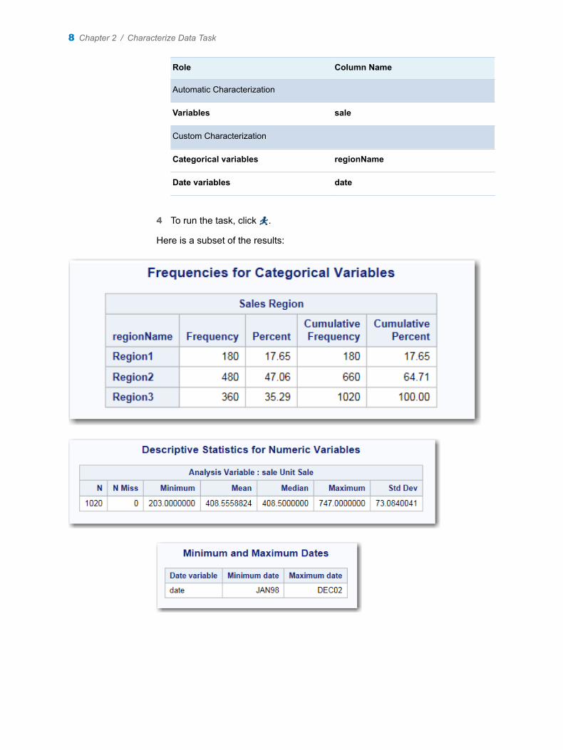
Role Column Name
Automatic Characterization
Variables sale
Custom Characterization
Categorical variables regionName
Date variables date
4 To run the task, click .
Here is a subset of the results:
8 Chapter 2 / Characterize Data Task
Assigning Data to Roles
To run the Characterize Data task, you must select an input data source. To filter the input data source, click .
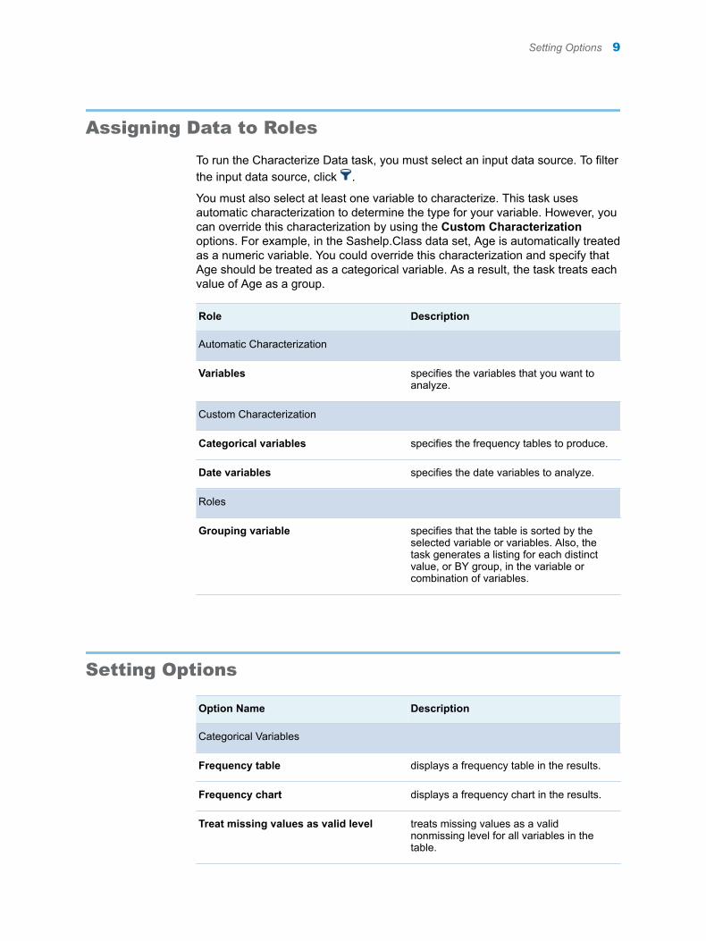
You must also select at least one variable to characterize. This task uses automatic characterization to determine the type for your variable. However, you can override this characterization by using the Custom Characterization options. For example, in the Sashelp.Class data set, Age is automatically treated as a numeric variable. You could override this characterization and specify that Age should be treated as a categorical variable. As a result, the task treats each value of Age as a group.
Role Description
Automatic Characterization
Variables specifies the variables that you want to analyze.
Custom Characterization
Categorical variables specifies the frequency tables to produce.
Date variables specifies the date variables to analyze.
Roles
Grouping variable specifies that the table is sorted by the selected variable or variables. Also, the task generates a listing for each distinct value, or BY group, in the variable or combination of variables.
Setting Options
Option Name Description
Categorical Variables
Frequency table displays a frequency table in the results.
Frequency chart displays a frequency chart in the results.
Treat missing values as valid level treats missing values as a valid nonmissing level for all variables in the table.
Setting Options 9
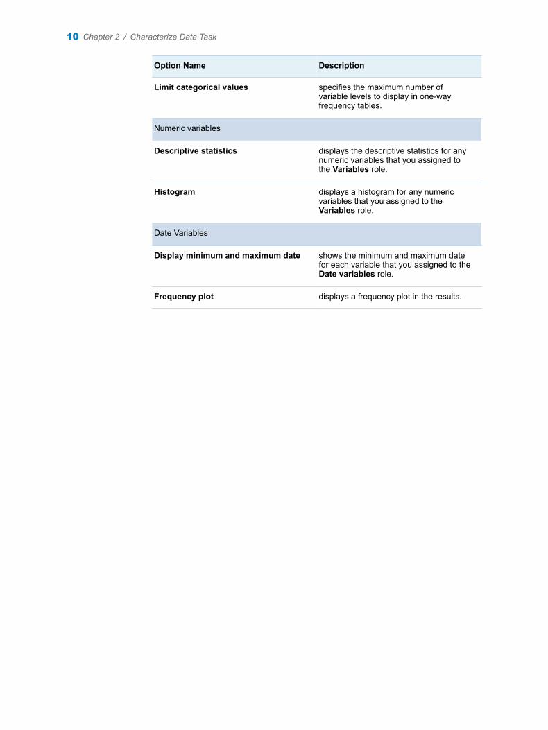
Option Name Description
Limit categorical values specifies the maximum number of variable levels to display in one-way frequency tables.
Numeric variables
Descriptive statistics displays the descriptive statistics for any numeric variables that you assigned to the Variables role.
Histogram displays a histogram for any numeric variables that you assigned to the Variables role.
Date Variables
Display minimum and maximum date shows the minimum and maximum date for each variable that you assigned to the Date variables role.
Frequency plot displays a frequency plot in the results.
10 Chapter 2 / Characterize Data Task

3Describe Missing Data
About the Describe Missing Data Task . . . . . . . . . . . . . . . . . . . . . . . . . . . . . . . . . . . . . . 11
Example: Describing Missing Data for SASHELP.BASEBALL . . . . . . . . . . . . . . . . 11
Setting the Data Options . . . . . . . . . . . . . . . . . . . . . . . . . . . . . . . . . . . . . . . . . . . . . . . . . . . . 13
About the Describe Missing Data Task
The Describe Missing Data task displays the frequencies and percentages of missing values for each selected variable. If two or more variables are assigned to this task, the task displays the pattern of missing data across variables.
Example: Describing Missing Data for SASHELP.BASEBALL
1 In the Tasks section, expand the Data folder, and then double-click Describe Missing Data. The user interface for the Describe Missing Data task opens.
2 On the Data tab, select SASHELP.BASEBALL as the input data set.
TIP If the data set is not available from the drop-down list, click . In
the Choose a Table window, expand the library that contains the data set that you want to use. Select the data set for the example and click OK. The selected data set should now appear in the drop-down list.
3 To the Analysis variables role, assign Salary and Div.
4 To run the task, click .
11
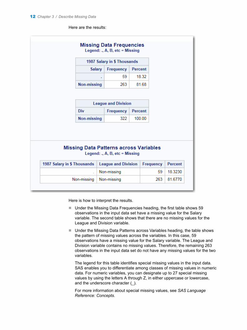
Here are the results:
Here is how to interpret the results.
n Under the Missing Data Frequencies heading, the first table shows 59 observations in the input data set have a missing value for the Salary variable. The second table shows that there are no missing values for the League and Division variable.
n Under the Missing Data Patterns across Variables heading, the table shows the pattern of missing values across the variables. In this case, 59 observations have a missing value for the Salary variable. The League and Division variable contains no missing values. Therefore, the remaining 263 observations in the input data set do not have any missing values for the two variables.
The legend for this table identifies special missing values in the input data. SAS enables you to differentiate among classes of missing values in numeric data. For numeric variables, you can designate up to 27 special missing values by using the letters A through Z, in either uppercase or lowercase, and the underscore character (_).
For more information about special missing values, see SAS Language Reference: Concepts.
12 Chapter 3 / Describe Missing Data
Setting the Data Options
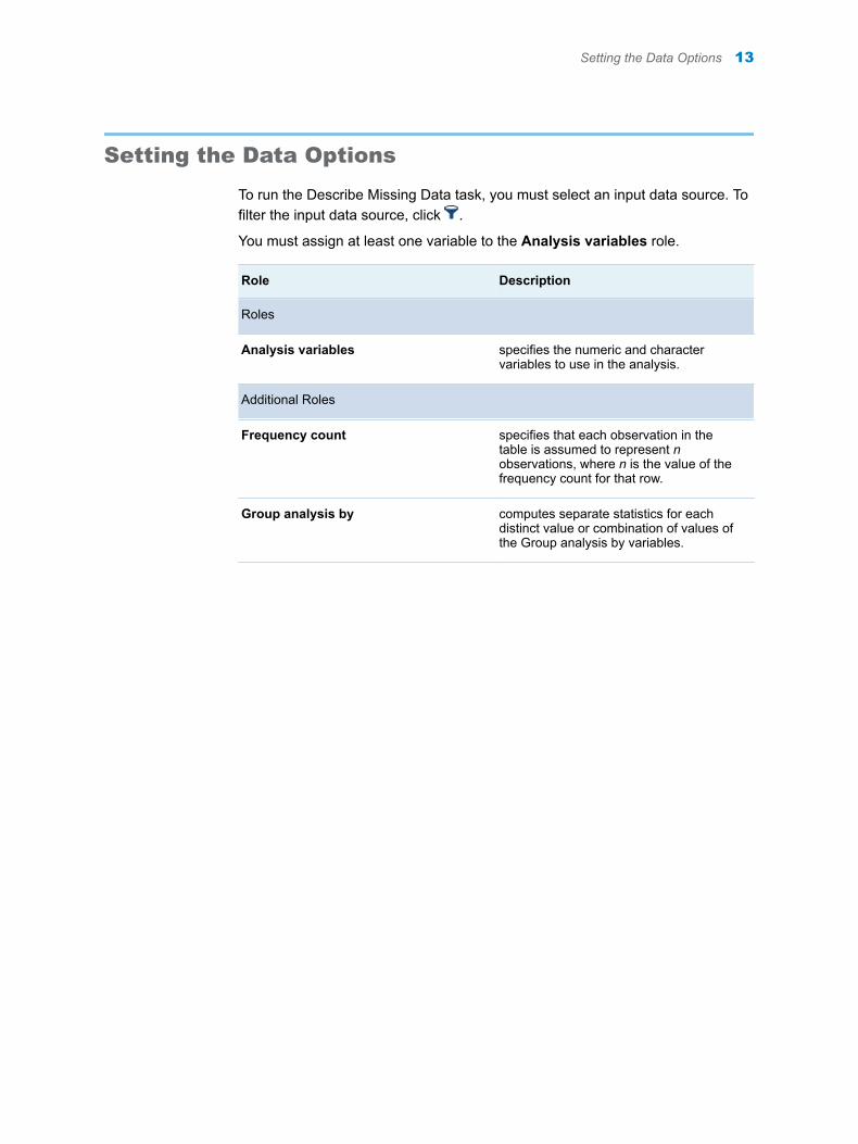
To run the Describe Missing Data task, you must select an input data source. To filter the input data source, click .
You must assign at least one variable to the Analysis variables role.
Role Description
Roles
Analysis variables specifies the numeric and character variables to use in the analysis.
Additional Roles
Frequency count specifies that each observation in the table is assumed to represent n observations, where n is the value of the frequency count for that row.
Group analysis by computes separate statistics for each distinct value or combination of values of the Group analysis by variables.
Setting the Data Options 13

14 Chapter 3 / Describe Missing Data
4List Data
About the List Data Task . . . . . . . . . . . . . . . . . . . . . . . . . . . . . . . . . . . . . . . . . . . . . . . . . . . . 15
Example: Reports of Drive Train, MSRP, and Engine Size by Car Type . . . . . . . 15
Assigning Data to Roles . . . . . . . . . . . . . . . . . . . . . . . . . . . . . . . . . . . . . . . . . . . . . . . . . . . . 17
Setting Options . . . . . . . . . . . . . . . . . . . . . . . . . . . . . . . . . . . . . . . . . . . . . . . . . . . . . . . . . . . . . 17
About the List Data Task
The List Data task displays the contents of a table as a report. For example, you can use the List Data task to create a report that sums the expenses and revenues for each sales region.
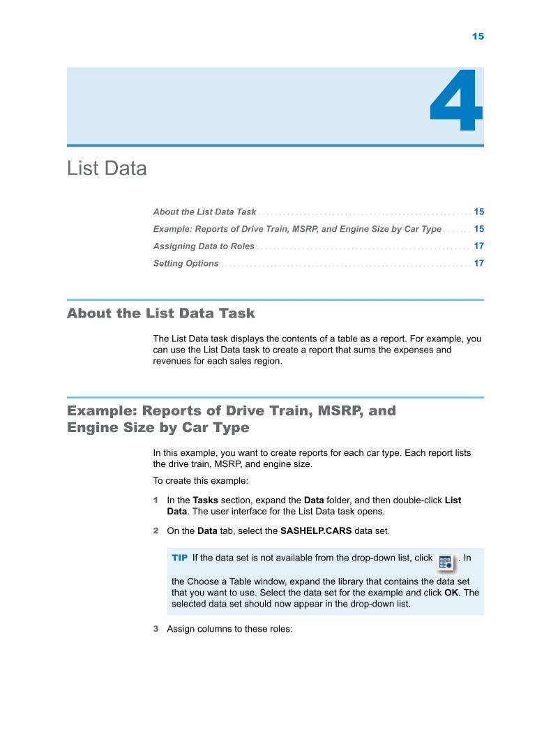
Example: Reports of Drive Train, MSRP, and Engine Size by Car Type
In this example, you want to create reports for each car type. Each report lists the drive train, MSRP, and engine size.
To create this example:
1 In the Tasks section, expand the Data folder, and then double-click List Data. The user interface for the List Data task opens.
2 On the Data tab, select the SASHELP.CARS data set.
TIP If the data set is not available from the drop-down list, click . In
the Choose a Table window, expand the library that contains the data set that you want to use. Select the data set for the example and click OK. The selected data set should now appear in the drop-down list.
3 Assign columns to these roles:
15
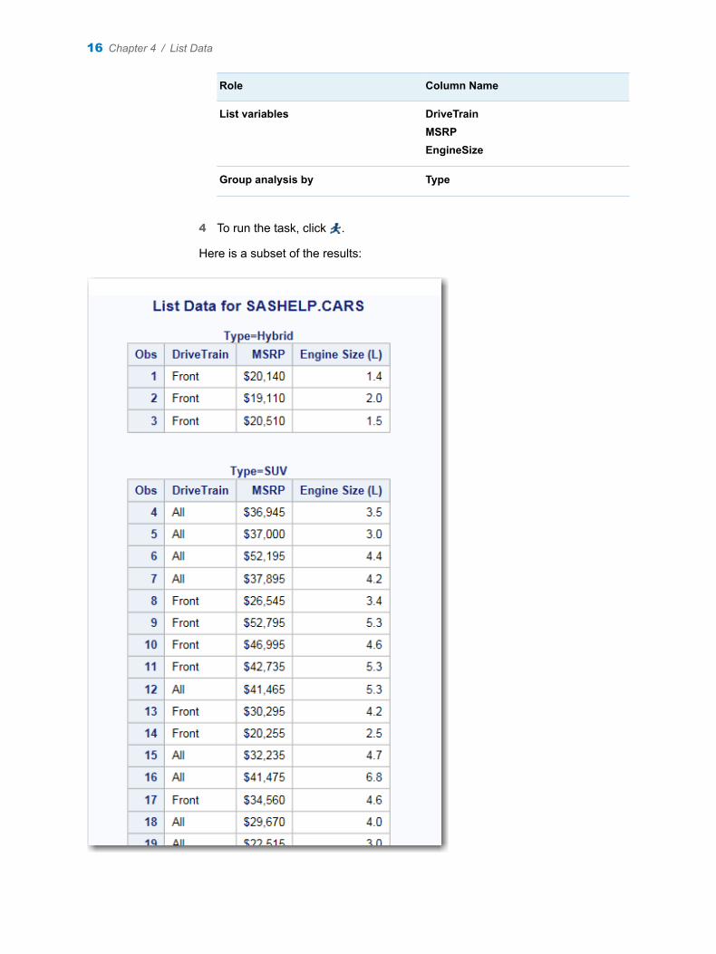
Role Column Name
List variables DriveTrainMSRPEngineSize
Group analysis by Type
4 To run the task, click .
Here is a subset of the results:
16 Chapter 4 / List Data
Assigning Data to Roles
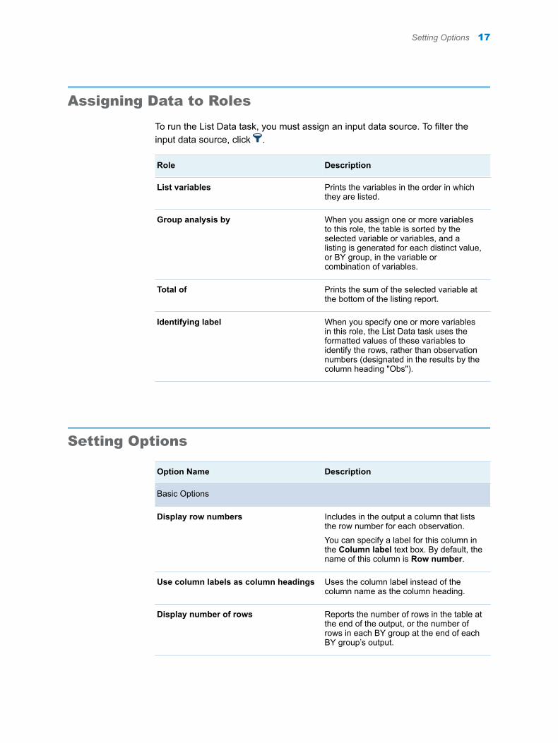
To run the List Data task, you must assign an input data source. To filter the input data source, click .
Role Description
List variables Prints the variables in the order in which they are listed.
Group analysis by When you assign one or more variables to this role, the table is sorted by the selected variable or variables, and a listing is generated for each distinct value, or BY group, in the variable or combination of variables.
Total of Prints the sum of the selected variable at the bottom of the listing report.
Identifying label When you specify one or more variables in this role, the List Data task uses the formatted values of these variables to identify the rows, rather than observation numbers (designated in the results by the column heading "Obs").
Setting Options
Option Name Description
Basic Options
Display row numbers Includes in the output a column that lists the row number for each observation.
You can specify a label for this column in the Column label text box. By default, the name of this column is Row number.
Use column labels as column headings Uses the column label instead of the column name as the column heading.
Display number of rows Reports the number of rows in the table at the end of the output, or the number of rows in each BY group at the end of each BY group’s output.
Setting Options 17
Option Name Description
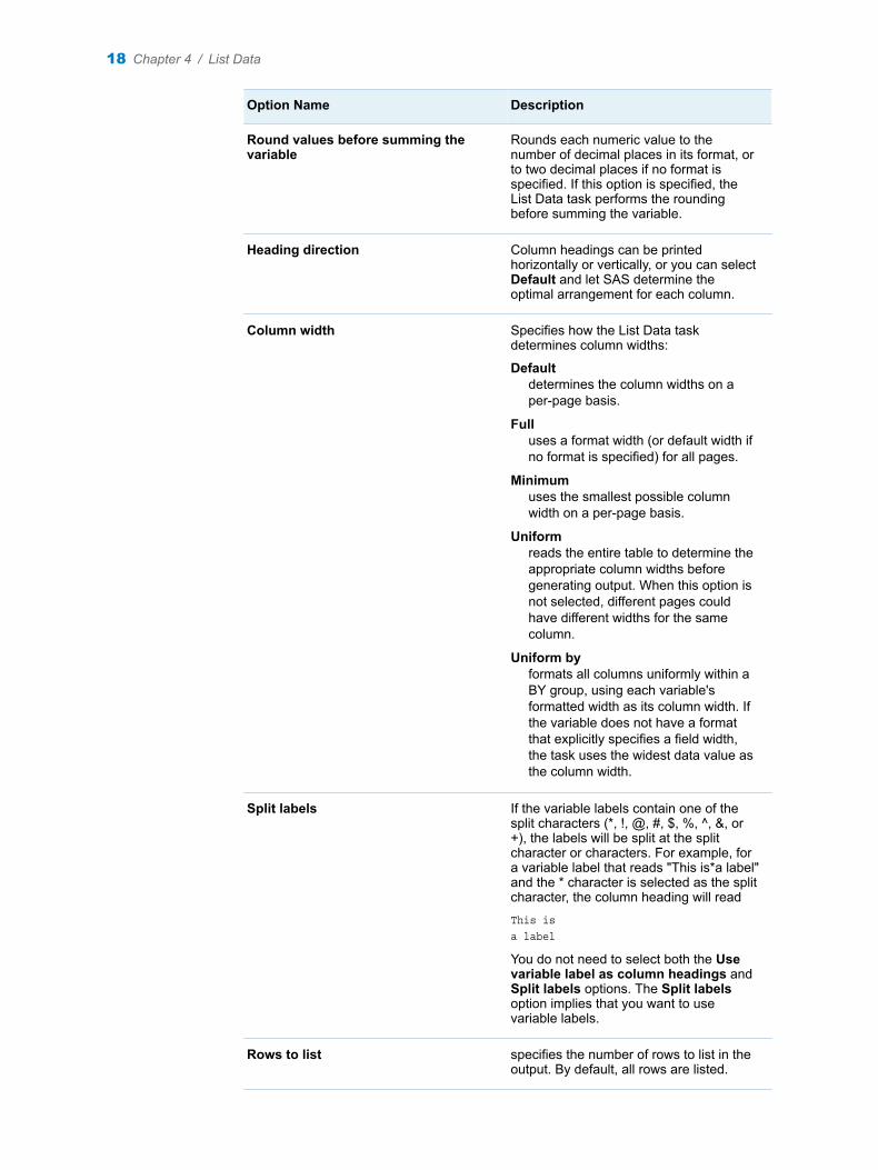
Round values before summing the variable
Rounds each numeric value to the number of decimal places in its format, or to two decimal places if no format is specified. If this option is specified, the List Data task performs the rounding before summing the variable.
Heading direction Column headings can be printed horizontally or vertically, or you can select Default and let SAS determine the optimal arrangement for each column.
Column width Specifies how the List Data task determines column widths:
Defaultdetermines the column widths on a per-page basis.
Fulluses a format width (or default width if no format is specified) for all pages.
Minimumuses the smallest possible column width on a per-page basis.
Uniformreads the entire table to determine the appropriate column widths before generating output. When this option is not selected, different pages could have different widths for the same column.
Uniform byformats all columns uniformly within a BY group, using each variable's formatted width as its column width. If the variable does not have a format that explicitly specifies a field width, the task uses the widest data value as the column width.
Split labels If the variable labels contain one of the split characters (*, !, @, #, $, %, ^, &, or +), the labels will be split at the split character or characters. For example, for a variable label that reads "This is*a label" and the * character is selected as the split character, the column heading will readThis isa label
You do not need to select both the Use variable label as column headings and Split labels options. The Split labels option implies that you want to use variable labels.
Rows to list specifies the number of rows to list in the output. By default, all rows are listed.
18 Chapter 4 / List Data

Setting Options 19

20 Chapter 4 / List Data
5Transpose Data
About the Transpose Data Task . . . . . . . . . . . . . . . . . . . . . . . . . . . . . . . . . . . . . . . . . . . . . 21
Example: Transposing the Data in the CLASS Data Set . . . . . . . . . . . . . . . . . . . . . . 21
Assigning Data to Roles . . . . . . . . . . . . . . . . . . . . . . . . . . . . . . . . . . . . . . . . . . . . . . . . . . . . 22
Setting Options . . . . . . . . . . . . . . . . . . . . . . . . . . . . . . . . . . . . . . . . . . . . . . . . . . . . . . . . . . . . . 23
About the Transpose Data Task
The Transpose Data task turns selected columns of an input table into the rows of an output table. If you do not use grouping variables, then each selected column is turned into a single row. If you use grouping variables, then the selected columns are divided into subcolumns based on the values of the grouping variables. Each subcolumn is turned into a row of the output table.
Example: Transposing the Data in the CLASS Data Set
1 In the Tasks section, expand the Data folder, and then double-click Transpose Data. The user interface for the Transpose Data task opens.
2 On the Data tab, select SASHELP.CLASS as the input data set.
3 To the Variables to transpose role, assign the Age, Height, and Weight variables.
4 Under the Output Data Set heading, select the Show output data check box.
5 On the Options tab, complete these steps:
a Clear the Use prefix check box.
b Select the Select a variable that contains the names of the new variables check box.
c To the New column names role, assign the Name variable.
6 To run the task, click .
21

The output data set contains a column for each student in the Sashelp.Class data set. The rows of the table are Age, Height, and Weight.
Assigning Data to Roles
To run the Transpose Data task, you must select an input data source. To filter the input data source, click .
You must assign a column to the Variables to transpose role.
Roles Description
Roles
Variables to transpose Each variable that you assign to this role becomes one or more rows of the output table. If you do not select any grouping variables, then an entire column is turned into a single row. If you select one or more grouping variables, then the grouping variables are used to segment each column into subcolumns, each of which is turned into a row. In this case, a column is transposed to the number of rows that is equal to the number of groups that are defined by the grouping variables.
You must assign at least one column to the Transpose variables role. To select a grouping variable, assign a column to the Group analysis by role.
Additional Roles
Group analysis by Each variable that you assign to this role is used to segment the about-to-be-transposed columns into subcolumns that will be transposed separately. Each subcolumn, defined by a set of values of the grouping variables, becomes a row of the output table.
Output Data Set
22 Chapter 5 / Transpose Data
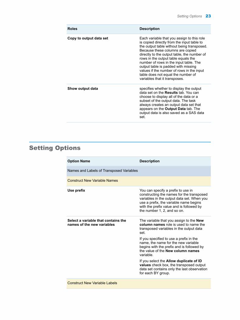
Roles Description
Copy to output data set Each variable that you assign to this role is copied directly from the input table to the output table without being transposed. Because these columns are copied directly to the output table, the number of rows in the output table equals the number of rows in the input table. The output table is padded with missing values if the number of rows in the input table does not equal the number of variables that it transposes.
Show output data specifies whether to display the output data set on the Results tab. You can choose to display all of the data or a subset of the output data. The task always creates an output data set that appears on the Output Data tab. The output data is also saved as a SAS data set.
Setting Options
Option Name Description
Names and Labels of Transposed Variables
Construct New Variable Names
Use prefix You can specify a prefix to use in constructing the names for the transposed variables in the output data set. When you use a prefix, the variable name begins with the prefix value and is followed by the number 1, 2, and so on.
Select a variable that contains the names of the new variables
The variable that you assign to the New column names role is used to name the transposed variables in the output data set.
If you specified to use a prefix in the name, the name for the new variable begins with the prefix and is followed by the value of the New column names variable.
If you select the Allow duplicate of ID values check box, the transposed output data set contains only the last observation for each BY group.
Construct New Variable Labels
Setting Options 23
Option Name Description
Select a variable that contains the labels of the new variables
The values of the variable that you assign to the New column labels role are used to label the variables in the output data set.
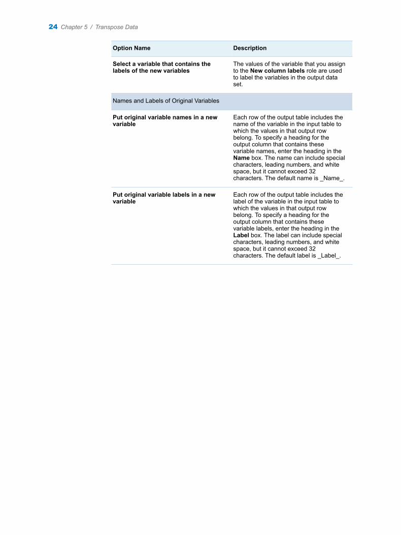
Names and Labels of Original Variables
Put original variable names in a new variable
Each row of the output table includes the name of the variable in the input table to which the values in that output row belong. To specify a heading for the output column that contains these variable names, enter the heading in the Name box. The name can include special characters, leading numbers, and white space, but it cannot exceed 32 characters. The default name is _Name_.
Put original variable labels in a new variable
Each row of the output table includes the label of the variable in the input table to which the values in that output row belong. To specify a heading for the output column that contains these variable labels, enter the heading in the Label box. The label can include special characters, leading numbers, and white space, but it cannot exceed 32 characters. The default label is _Label_.
24 Chapter 5 / Transpose Data
6Stack/Split Columns
About the Stack/Split Columns Task . . . . . . . . . . . . . . . . . . . . . . . . . . . . . . . . . . . . . . . . 25
Stacking Columns . . . . . . . . . . . . . . . . . . . . . . . . . . . . . . . . . . . . . . . . . . . . . . . . . . . . . . . . . . 26Example 1: Stacking Columns in the CLASSFIT Data Set . . . . . . . . . . . . . . . . . . . 26Example 2: Creating Multiple Stacked Columns . . . . . . . . . . . . . . . . . . . . . . . . . . . . . 27Create a Stacked Column . . . . . . . . . . . . . . . . . . . . . . . . . . . . . . . . . . . . . . . . . . . . . . . . . 29
Splitting Columns . . . . . . . . . . . . . . . . . . . . . . . . . . . . . . . . . . . . . . . . . . . . . . . . . . . . . . . . . . 30Example 1: Splitting the Height Column in the CLASSFIT Data Set . . . . . . . . . . . 30Example 2: Creating Multiple Split Columns . . . . . . . . . . . . . . . . . . . . . . . . . . . . . . . . 32Split a Column . . . . . . . . . . . . . . . . . . . . . . . . . . . . . . . . . . . . . . . . . . . . . . . . . . . . . . . . . . . 34
About the Stack/Split Columns Task
The Stack/Split Columns task enables you to either stack or split columns.
n When stacking columns, the output data set is created by restructuring the selected columns in the input data set so that these columns are transposed into observations. You can use the output data set to analyze values across multiple columns of the input data set. If you group the observations, the selected columns are divided into subgroups that are based on the unique combinations of the grouping values. Each subgroup forms a row of the output data set.
This functionality is useful when you have a data set in which each observation contains the same type of data in multiple columns and you want to analyze the data across several columns. For example, you could transpose columns that contain monthly temperature readings for various locations across a geographic region. The output data set would contain the monthly temperature readings by location in a single column.
n When splitting columns, the output data set is created by splitting the unique combination of values of the selected columns. You can use the output data set to individually analyze the columns that contain multiple rows of the input data set.
This functionality is useful when you have a data set in which one column contains multiple observations for different subgroups and you want to split the subgroup measures into separate columns. For example, you could transpose a column that contains the monthly temperature readings for various locations across a geographic region. The output data set would
25
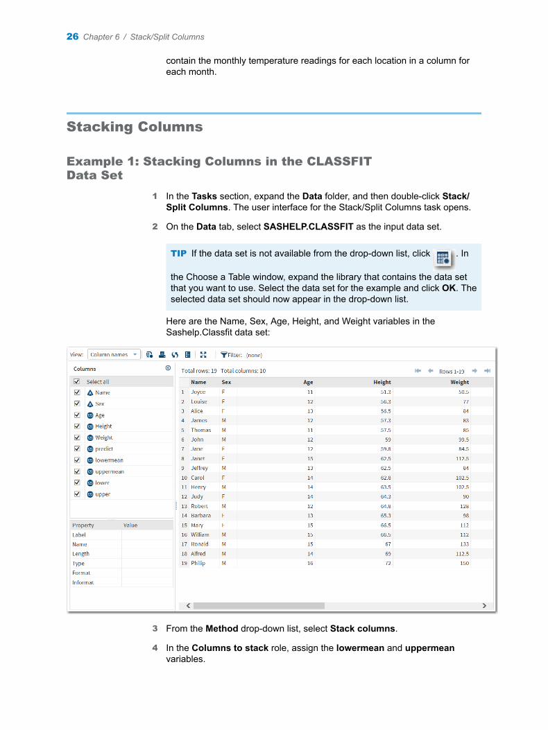
contain the monthly temperature readings for each location in a column for each month.
Stacking Columns
Example 1: Stacking Columns in the CLASSFIT Data Set
1 In the Tasks section, expand the Data folder, and then double-click Stack/Split Columns. The user interface for the Stack/Split Columns task opens.
2 On the Data tab, select SASHELP.CLASSFIT as the input data set.
TIP If the data set is not available from the drop-down list, click . In
the Choose a Table window, expand the library that contains the data set that you want to use. Select the data set for the example and click OK. The selected data set should now appear in the drop-down list.
Here are the Name, Sex, Age, Height, and Weight variables in the Sashelp.Classfit data set:
3 From the Method drop-down list, select Stack columns.
4 In the Columns to stack role, assign the lowermean and uppermean variables.
26 Chapter 6 / Stack/Split Columns

5 On the Output tab, enter CLM as the name of the new column.
6 Assign these variables to the Include other variables in output data set role.
n Name
n Sex
n Age
n Height
n Weight
n predict
7 To run the task, click .
The results contain three new variables: _Case_, _Level_, and CLM. The _Case_ variable contains the case identifier. A case is the data for an individual student. The _Level_ variable contains the names of the stacked columns. The new CLM variable contains the value of the lower mean or upper mean.
Example 2: Creating Multiple Stacked Columns
Using the Stack/Split Columns task, you can create multiple stacked variables.
1 In SAS Studio, click and select New SAS Program.
2 To create the multistack data set, copy and paste this code onto the Program tab.
Stacking Columns 27
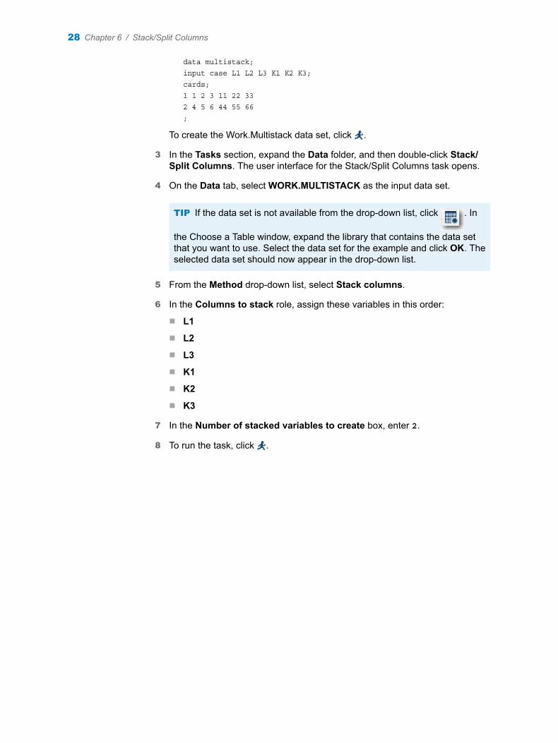
data multistack;input case L1 L2 L3 K1 K2 K3;cards;1 1 2 3 11 22 332 4 5 6 44 55 66;
To create the Work.Multistack data set, click .
3 In the Tasks section, expand the Data folder, and then double-click Stack/Split Columns. The user interface for the Stack/Split Columns task opens.
4 On the Data tab, select WORK.MULTISTACK as the input data set.
TIP If the data set is not available from the drop-down list, click . In
the Choose a Table window, expand the library that contains the data set that you want to use. Select the data set for the example and click OK. The selected data set should now appear in the drop-down list.
5 From the Method drop-down list, select Stack columns.
6 In the Columns to stack role, assign these variables in this order:
n L1
n L2
n L3
n K1
n K2
n K3
7 In the Number of stacked variables to create box, enter 2.
8 To run the task, click .
28 Chapter 6 / Stack/Split Columns
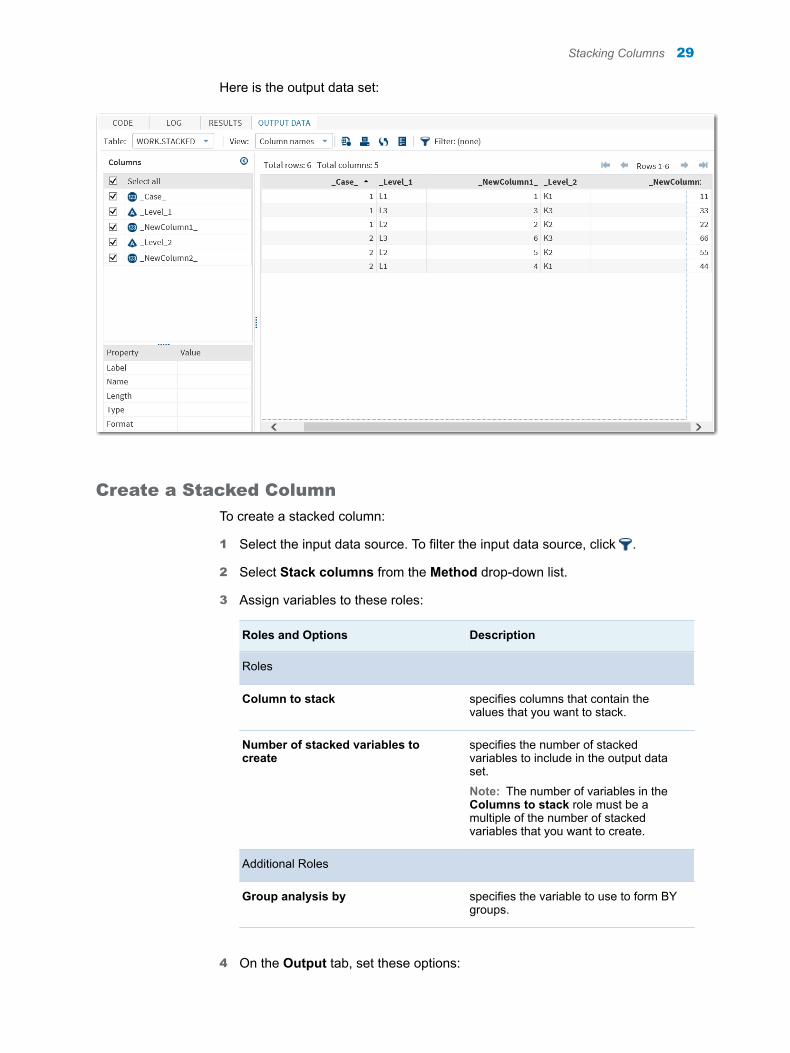
Here is the output data set:
Create a Stacked Column
To create a stacked column:
1 Select the input data source. To filter the input data source, click .
2 Select Stack columns from the Method drop-down list.
3 Assign variables to these roles:
Roles and Options Description
Roles
Column to stack specifies columns that contain the values that you want to stack.
Number of stacked variables to create
specifies the number of stacked variables to include in the output data set.
Note: The number of variables in the Columns to stack role must be a multiple of the number of stacked variables that you want to create.
Additional Roles
Group analysis by specifies the variable to use to form BY groups.
4 On the Output tab, set these options:
Stacking Columns 29

Option Name Description
Output Data Set
Name of new column specifies the name of the new column that contains all the stacked values.
Case Identifier
Case identifier specifies the name of the new column that contains the values that identify a particular case. You can select whether the task creates a case variable, or you can select identifier variables from the input data set.
New column name of case identifier specifies the name of the new column that contains the values of the case identifier.
Level Identifier
Name of column containing levels of stacked columns
specifies the name of the new column that contains the levels.
Include other variables in output data set
enables you to select other variables from the input data set that you want to include in the output data set.
Show Output Data Set
Show output data specifies whether to display the output data set on the Results tab. You can choose to display all of the data or a subset of the output data. The task always creates an output data set that appears on the Output Data tab. The output data is also saved as a SAS data set.
Splitting Columns
Example 1: Splitting the Height Column in the CLASSFIT Data Set
1 In the Tasks section, expand the Data folder, and then double-click Stack/Split Columns. The user interface for the Stack/Split Columns task opens.
2 On the Data tab, select SASHELP.CLASSFIT as the input data set.
30 Chapter 6 / Stack/Split Columns
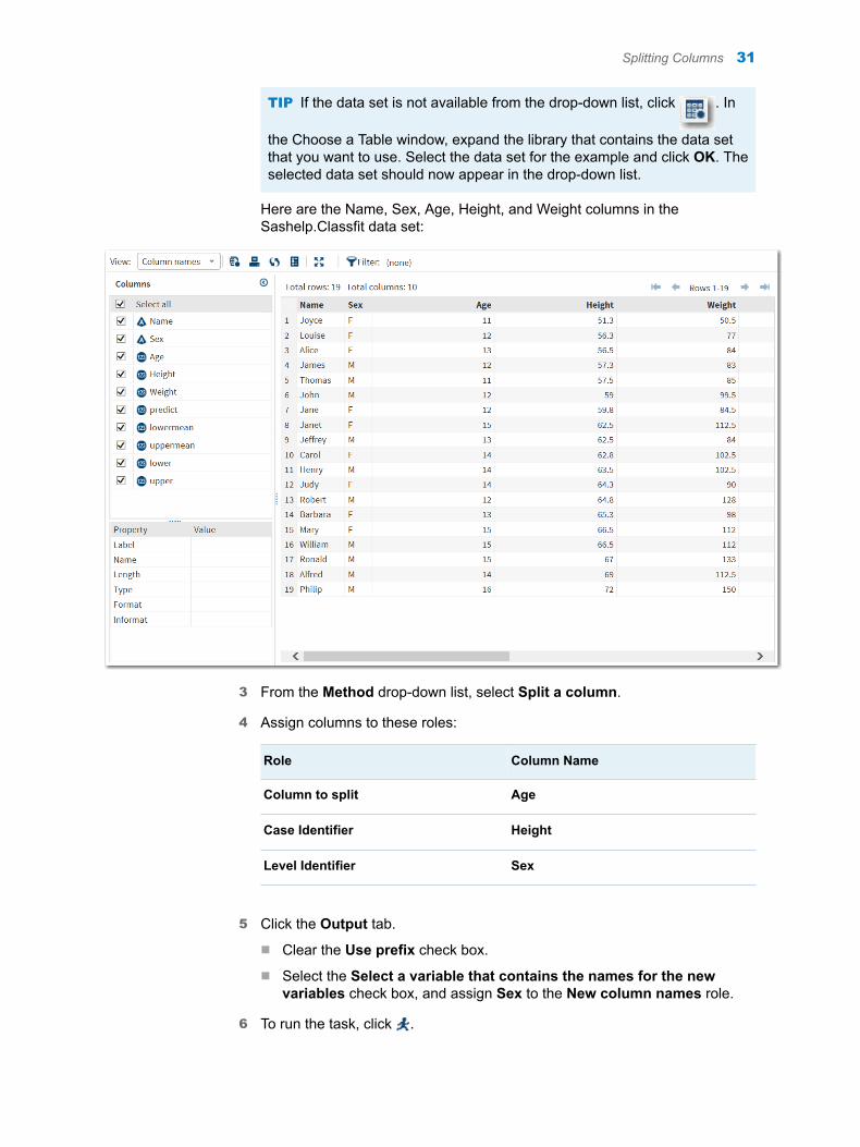
TIP If the data set is not available from the drop-down list, click . In
the Choose a Table window, expand the library that contains the data set that you want to use. Select the data set for the example and click OK. The selected data set should now appear in the drop-down list.
Here are the Name, Sex, Age, Height, and Weight columns in the Sashelp.Classfit data set:
3 From the Method drop-down list, select Split a column.
4 Assign columns to these roles:
Role Column Name
Column to split Age
Case Identifier Height
Level Identifier Sex
5 Click the Output tab.
n Clear the Use prefix check box.
n Select the Select a variable that contains the names for the new variables check box, and assign Sex to the New column names role.
6 To run the task, click .
Splitting Columns 31
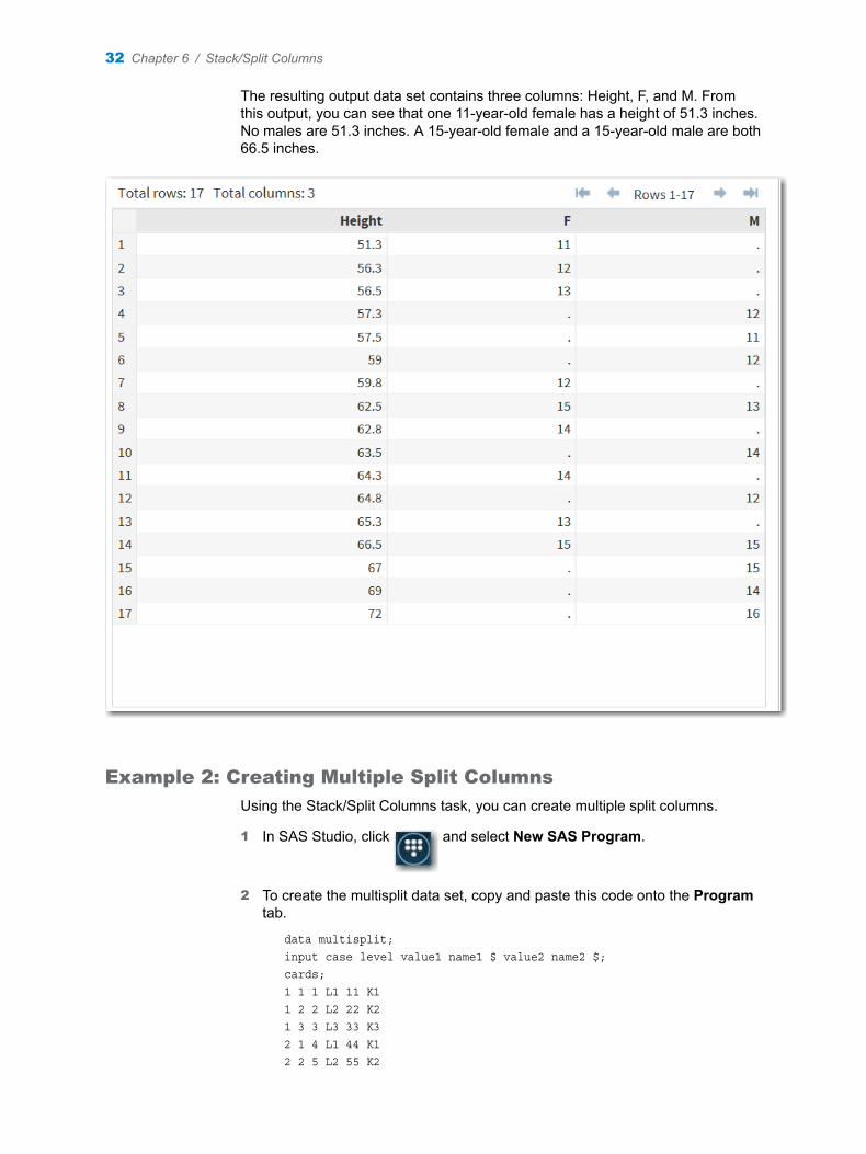
The resulting output data set contains three columns: Height, F, and M. From this output, you can see that one 11-year-old female has a height of 51.3 inches. No males are 51.3 inches. A 15-year-old female and a 15-year-old male are both 66.5 inches.
Example 2: Creating Multiple Split Columns
Using the Stack/Split Columns task, you can create multiple split columns.
1 In SAS Studio, click and select New SAS Program.
2 To create the multisplit data set, copy and paste this code onto the Program tab.
data multisplit;input case level value1 name1 $ value2 name2 $;cards;1 1 1 L1 11 K11 2 2 L2 22 K21 3 3 L3 33 K32 1 4 L1 44 K12 2 5 L2 55 K2
32 Chapter 6 / Stack/Split Columns
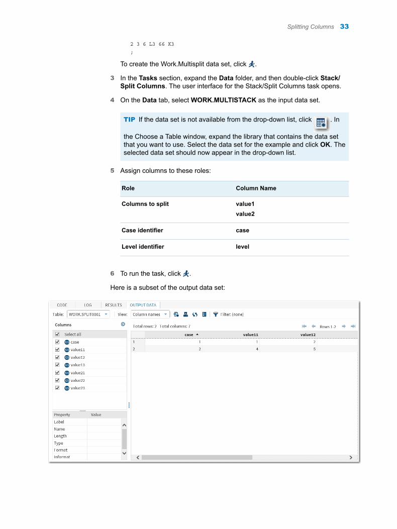
2 3 6 L3 66 K3;
To create the Work.Multisplit data set, click .
3 In the Tasks section, expand the Data folder, and then double-click Stack/Split Columns. The user interface for the Stack/Split Columns task opens.
4 On the Data tab, select WORK.MULTISTACK as the input data set.
TIP If the data set is not available from the drop-down list, click . In
the Choose a Table window, expand the library that contains the data set that you want to use. Select the data set for the example and click OK. The selected data set should now appear in the drop-down list.
5 Assign columns to these roles:
Role Column Name
Columns to split value1value2
Case identifier case
Level identifier level
6 To run the task, click .
Here is a subset of the output data set:
Splitting Columns 33
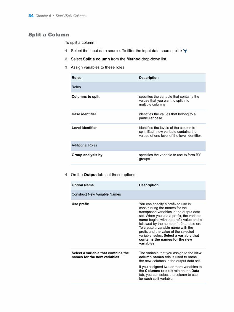
Split a Column
To split a column:
1 Select the input data source. To filter the input data source, click .
2 Select Split a column from the Method drop-down list.
3 Assign variables to these roles:
Roles Description
Roles
Columns to split specifies the variable that contains the values that you want to split into multiple columns.
Case identifier identifies the values that belong to a particular case.
Level identifier identifies the levels of the column to split. Each new variable contains the values of one level of the level identifier.
Additional Roles
Group analysis by specifies the variable to use to form BY groups.
4 On the Output tab, set these options:
Option Name Description
Construct New Variable Names
Use prefix You can specify a prefix to use in constructing the names for the transposed variables in the output data set. When you use a prefix, the variable name begins with the prefix value and is followed by the number 1, 2, and so on. To create a variable name with the prefix and the value of the selected variable, select Select a variable that contains the names for the new variables.
Select a variable that contains the names for the new variables
The variable that you assign to the New column names role is used to name the new columns in the output data set.
If you assigned two or more variables to the Columns to split role on the Data tab, you can select the column to use for each split variable.
34 Chapter 6 / Stack/Split Columns
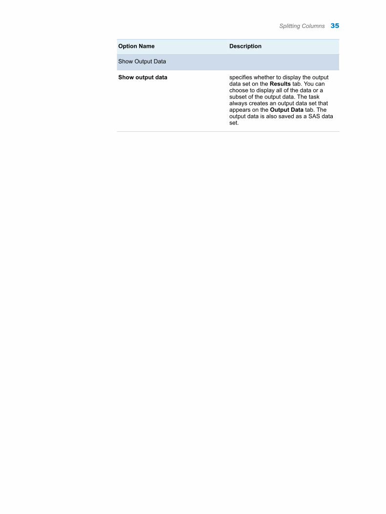
Option Name Description
Show Output Data
Show output data specifies whether to display the output data set on the Results tab. You can choose to display all of the data or a subset of the output data. The task always creates an output data set that appears on the Output Data tab. The output data is also saved as a SAS data set.
Splitting Columns 35

36 Chapter 6 / Stack/Split Columns
7Filter Data
About the Filter Data Task . . . . . . . . . . . . . . . . . . . . . . . . . . . . . . . . . . . . . . . . . . . . . . . . . . 37
Example 1: Creating a Simple Filter . . . . . . . . . . . . . . . . . . . . . . . . . . . . . . . . . . . . . . . . . 37
Example 2: Creating a Compound Filter . . . . . . . . . . . . . . . . . . . . . . . . . . . . . . . . . . . . . 38
Creating Your Filter . . . . . . . . . . . . . . . . . . . . . . . . . . . . . . . . . . . . . . . . . . . . . . . . . . . . . . . . . 39
About the Filter Data Task
The Filter Data task enables you to quickly create a basic filter to subset your input data source. You can use just one variable in a filter, or you can use multiple variables to create several comparison expressions. If you create more than one comparison expression in your filter, you specify whether the relationship between the filter elements is AND or OR. The filter elements are evaluated in the order in which they appear in the user interface. To change this order, you can add parentheses to the code generated by the task.
Example 1: Creating a Simple Filter
This example creates an output data set that contains salaries less than $750,000.
1 In the Tasks section, expand the Data folder, and then double-click Filter Data. The user interface for the Filter Data task opens.
2 For the input data source, select SASHELP.BASEBALL.
3 To the Variable 1 role, assign Salary.
4 From the Comparison drop-down list, select Less than.
5 From the Value type drop-down list, select Enter a value.
6 In the Value box, enter 750.
7 Under the Output Data Set heading, select Show output data to view the output data set in the results. From the Show drop-down list, select Show all output data.
37
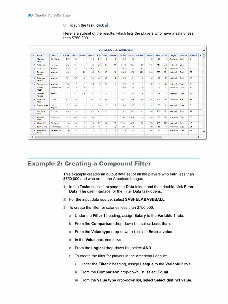
8 To run the task, click .
Here is a subset of the results, which lists the players who have a salary less than $750,000.
Example 2: Creating a Compound Filter
This example creates an output data set of all the players who earn less than $750,000 and who are in the American League.
1 In the Tasks section, expand the Data folder, and then double-click Filter Data. The user interface for the Filter Data task opens.
2 For the input data source, select SASHELP.BASEBALL.
3 To create the filter for salaries less than $750,000:
a Under the Filter 1 heading, assign Salary to the Variable 1 role.
b From the Comparison drop-down list, select Less than.
c From the Value type drop-down list, select Enter a value.
d In the Value box, enter 750.
e From the Logical drop-down list, select AND.
f To create the filter for players in the American League:
i Under the Filter 2 heading, assign League to the Variable 2 role.
ii From the Comparison drop-down list, select Equal.
iii From the Value type drop-down list, select Select distinct value.
38 Chapter 7 / Filter Data
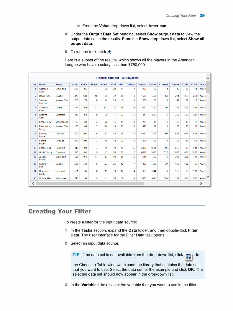
iv From the Value drop-down list, select American.
4 Under the Output Data Set heading, select Show output data to view the output data set in the results. From the Show drop-down list, select Show all output data.
5 To run the task, click .
Here is a subset of the results, which shows all the players in the American League who have a salary less than $750,000.
Creating Your Filter
To create a filter for the input data source:
1 In the Tasks section, expand the Data folder, and then double-click Filter Data. The user interface for the Filter Data task opens.
2 Select an input data source.
TIP If the data set is not available from the drop-down list, click . In
the Choose a Table window, expand the library that contains the data set that you want to use. Select the data set for the example and click OK. The selected data set should now appear in the drop-down list.
3 In the Variable 1 box, select the variable that you want to use in the filter.
Creating Your Filter 39

4 From the Comparison drop-down list, select the comparison operator. The default value is Less than.
5 From the Value type drop-down list, choose one of these options:
n Enter value specifies that you want to enter a value in the Value box.
n Select distinct value specifies that you want to select a value from the input data source. The Value drop-down list shows the first 100 unique values for that column.
n Enter a percentile specifies that you want to enter a percentage in the Value box.
6 To create a compound filter, select a value from the Logical drop-down list. Then specify the values for Filter 2.
7 To specify a name for the output data set, expand Output Data Set and enter the name for the output data set in the Data box. You can select the variables to include in the output data set.
To view the output data in the results, select Show output data. You can choose to view a subset or all of the data.
40 Chapter 7 / Filter Data
8Select Random Sample
About the Select Random Sample Task . . . . . . . . . . . . . . . . . . . . . . . . . . . . . . . . . . . . . 41
Example: Creating a Random Sample of the Sashelp.Pricedata Data Set . . . . 41
Assigning Data to Roles . . . . . . . . . . . . . . . . . . . . . . . . . . . . . . . . . . . . . . . . . . . . . . . . . . . . 43
Setting Options . . . . . . . . . . . . . . . . . . . . . . . . . . . . . . . . . . . . . . . . . . . . . . . . . . . . . . . . . . . . . 45
About the Select Random Sample Task
The Select Random Sample task creates an output table that contains a random sample of the rows in the input table.
You might use this task when you need a subset of the data. For example, suppose you want to audit employee travel expenses in an effort to improve the expense reporting procedure and possibly reduce expenses. Because you do not have the resources to examine all expense reports, you can use statistical sampling to objectively select expense reports for audit.
Example: Creating a Random Sample of the Sashelp.Pricedata Data Set
In this example, you want to create a subset of the data in the Sashelp.Pricedata data set.
To create this example:
1 In the Tasks section, expand the Data folder, and then double-click Select Random Sample. The user interface for the Select Random Sample task opens.
2 On the Data tab, select the SASHELP.PRICEDATA data set.
TIP If the data set is not available from the drop-down list, click . In
the Choose a Table window, expand the library that contains the data set that you want to use. Select the data set for the example and click OK. The selected data set should now appear in the drop-down list.
41
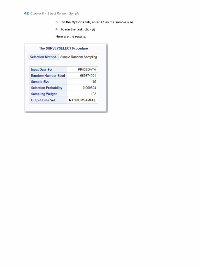
3 On the Options tab, enter 10 as the sample size.
4 To run the task, click .
Here are the results:
42 Chapter 8 / Select Random Sample
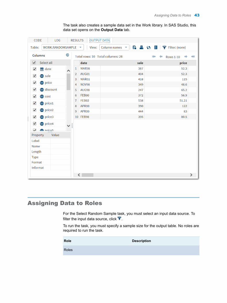
The task also creates a sample data set in the Work library. In SAS Studio, this data set opens on the Output Data tab.
Assigning Data to Roles
For the Select Random Sample task, you must select an input data source. To filter the input data source, click .
To run the task, you must specify a sample size for the output table. No roles are required to run the task.
Role Description
Roles
Assigning Data to Roles 43

Role Description
Stratify by specifies the variables to use to partition the input table into mutually exclusive, non-overlapping subsets that are known as strata. Each stratum is defined by a set of values of the strata variables, and each stratum is sampled separately. The complete sample is the union of the samples that are taken from all the strata.
Note: If you do not assign any variables to this role, then the entire input table is treated as a single stratum.
This example shows how the total sample size among the strata is in proportion to the size of the stratum. For this example, the variable GENDER has possible values of M and F, and the variable VOTED has possible values of Y and N. If you assign both GENDER and VOTED to the Strata columns role, then the input table is partitioned into four strata: males who voted, males who did not vote, females who voted, and females who did not vote.
The input table contains 20,000 rows, and the values are distributed as follows:
n 7,000 males who votedn 4,000 males who did not vote n 5,000 females who voted n 4,000 females who did not vote
Therefore, the proportion of males who voted is 7,000/20,000=0.35 or 35%. The proportions in the sample should reflect the proportions of the strata in the input table. For example, if your sample table contains 100 observations, then 35% of the values in the sample must be selected from the males who voted stratum to reflect the proportions in the input table.
Output Data Set
Data set name specifies the name of the output data set.
Include all variables in the output data set
specifies the variables to include in the output table. By default, all variables are included in the output table. However, you can select the variables to include in the output.
Show Output Data
Show specifies whether to include all of the data in the output data set or only a portion of the data.
44 Chapter 8 / Select Random Sample
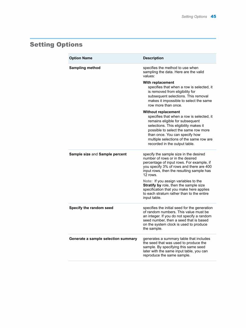
Setting Options
Option Name Description
Sampling method specifies the method to use when sampling the data. Here are the valid values:
With replacementspecifies that when a row is selected, it is removed from eligibility for subsequent selections. This removal makes it impossible to select the same row more than once.
Without replacementspecifies that when a row is selected, it remains eligible for subsequent selections. This eligibility makes it possible to select the same row more than once. You can specify how multiple selections of the same row are recorded in the output table.
Sample size and Sample percent specify the sample size in the desired number of rows or in the desired percentage of input rows. For example, if you specify 3% of rows and there are 400 input rows, then the resulting sample has 12 rows.
Note: If you assign variables to the Stratify by role, then the sample size specification that you make here applies to each stratum rather than to the entire input table.
Specify the random seed specifies the initial seed for the generation of random numbers. This value must be an integer. If you do not specify a random seed number, then a seed that is based on the system clock is used to produce the sample.
Generate a sample selection summary generates a summary table that includes the seed that was used to produce the sample. By specifying this same seed later with the same input table, you can reproduce the same sample.
Setting Options 45

46 Chapter 8 / Select Random Sample
9Partition Data
About the Partition Data Task . . . . . . . . . . . . . . . . . . . . . . . . . . . . . . . . . . . . . . . . . . . . . . . 47
Example: Partitioning the SASHELP.CLASSFIT Data Set . . . . . . . . . . . . . . . . . . . . 47
Creating a Partitioned Data Set . . . . . . . . . . . . . . . . . . . . . . . . . . . . . . . . . . . . . . . . . . . . . 48
About the Partition Data Task
A partition is all or part of a logical file. The Partition Data task enables you to create up to four partitions created by randomly sampling the input data. Partitions can be used to develop a model. In this case, you want to train the model on part of the data and reserve some of the data for testing. Using the Partition Data task, you can save all the partitions to one output data set or save each partition in a separate data set.
Example: Partitioning the SASHELP.CLASSFIT Data Set
1 In the Tasks section, expand the Data folder, and then double-click Partition Data. The user interface for the Partition Data task opens.
2 On the Data tab, select SASHELP.CLASSFIT as the input data set.
TIP If the data set is not available from the drop-down list, click . In
the Choose a Table window, expand the library that contains the data set that you want to use. Select the data set for the example and click OK. The selected data set should now appear in the drop-down list.
3 In the Number of partitions box, enter 2.
4 In the Proportion of cases for partition 1 box, enter .5, which specifies 50% of the values should be in partition 1.
5 In the Proportion of cases for partition 2 box, enter .3, which specifies 30% of the values should be in partition 2.
47
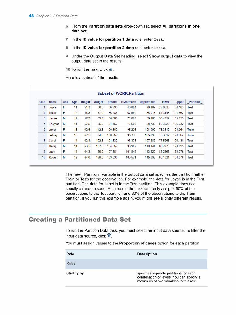
6 From the Partition data sets drop-down list, select All partitions in one data set.
7 In the ID value for partition 1 data role, enter Test.
8 In the ID value for partition 2 data role, enter Train.
9 Under the Output Data Set heading, select Show output data to view the output data set in the results.
10 To run the task, click .
Here is a subset of the results:
The new _Partition_ variable in the output data set specifies the partition (either Train or Test) for the observation. For example, the data for Joyce is in the Test partition. The data for Janet is in the Test partition. This example does not specify a random seed. As a result, the task randomly assigns 50% of the observations to the Test partition and 30% of the observations to the Train partition. If you run this example again, you might see slightly different results.
Creating a Partitioned Data Set
To run the Partition Data task, you must select an input data source. To filter the input data source, click .
You must assign values to the Proportion of cases option for each partition.
Role Description
Roles
Stratify by specifies separate partitions for each combination of levels. You can specify a maximum of two variables to this role.
48 Chapter 9 / Partition Data
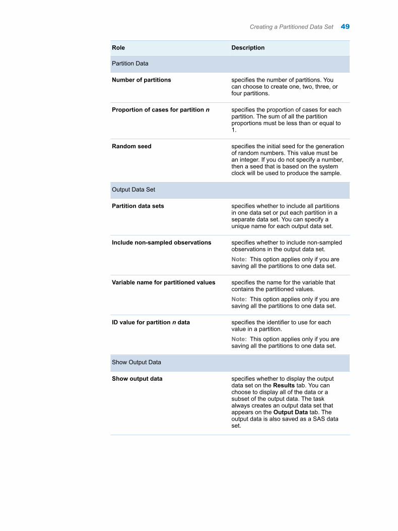
Role Description
Partition Data
Number of partitions specifies the number of partitions. You can choose to create one, two, three, or four partitions.
Proportion of cases for partition n specifies the proportion of cases for each partition. The sum of all the partition proportions must be less than or equal to 1.
Random seed specifies the initial seed for the generation of random numbers. This value must be an integer. If you do not specify a number, then a seed that is based on the system clock will be used to produce the sample.
Output Data Set
Partition data sets specifies whether to include all partitions in one data set or put each partition in a separate data set. You can specify a unique name for each output data set.
Include non-sampled observations specifies whether to include non-sampled observations in the output data set.
Note: This option applies only if you are saving all the partitions to one data set.
Variable name for partitioned values specifies the name for the variable that contains the partitioned values.
Note: This option applies only if you are saving all the partitions to one data set.
ID value for partition n data specifies the identifier to use for each value in a partition.
Note: This option applies only if you are saving all the partitions to one data set.
Show Output Data
Show output data specifies whether to display the output data set on the Results tab. You can choose to display all of the data or a subset of the output data. The task always creates an output data set that appears on the Output Data tab. The output data is also saved as a SAS data set.
Creating a Partitioned Data Set 49

50 Chapter 9 / Partition Data
10Sort Data
About the Sort Data Task . . . . . . . . . . . . . . . . . . . . . . . . . . . . . . . . . . . . . . . . . . . . . . . . . . . 51
Example: Sort the SASHELP.CLASS Data Set by Sex and Age . . . . . . . . . . . . . . . 51
Assigning Data to Roles . . . . . . . . . . . . . . . . . . . . . . . . . . . . . . . . . . . . . . . . . . . . . . . . . . . . 52
Setting Options . . . . . . . . . . . . . . . . . . . . . . . . . . . . . . . . . . . . . . . . . . . . . . . . . . . . . . . . . . . . . 53
About the Sort Data Task
The Sort Data task enables you to sort the table by any of its columns. The result from this task is a sorted table in the Work library.
Example: Sort the SASHELP.CLASS Data Set by Sex and Age
To create this example:
1 In the Tasks section, expand the Data folder, and then double-click Sort Data. The user interface for the Sort Data task opens.
2 On the Data tab, select the SASHELP.CLASS data set.
TIP If the data set is not available from the drop-down list, click . In
the Choose a Table window, expand the library that contains the data set that you want to use. Select the data set for the example and click OK. The selected data set should now appear in the drop-down list.
3 To the Sort by role, assign the Sex and Age columns.
4 To run the task, click .
The newly created WORK.SortDS data set is available from the Output Data tab. In the output data, the observations are first sorted by Sex (whether Female
51
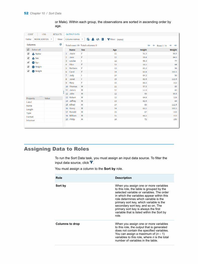
or Male). Within each group, the observations are sorted in ascending order by age.
Assigning Data to Roles
To run the Sort Data task, you must assign an input data source. To filter the input data source, click .
You must assign a column to the Sort by role.
Role Description
Sort by When you assign one or more variables to this role, the table is grouped by the selected variable or variables. The order in which the variables appear within this role determines which variable is the primary sort key, which variable is the secondary sort key, and so on. The primary sort key is always the first variable that is listed within the Sort by role.
Columns to drop When you assign one or more variables to this role, the output that is generated does not contain the specified variables. You can assign a maximum of (n – 1) variables to this role, where n is the total number of variables in the table.
52 Chapter 10 / Sort Data

Setting Options
Option Name Description
Output Order
Sort order specifies whether to display the output data in ascending or descending order.
Maintain original order within groups maintains the order of the observations relative to each other within a BY group.
Duplicate Records
Keep all records keeps all of the records that are in the output table, including all duplicate records.
Keep only the first record for each ‘Sort by’ group
eliminates any duplicate observations that have the same values for the Sort by group.
Results
Sort in place specifies to sort the existing data set in place. If you select this option, the Sort task keeps any variables that you assigned to the Columns to drop role and keeps all duplicate records.
Output data set specifies the name of the output data set.
Setting Options 53

54 Chapter 10 / Sort Data
11Rank Data
About the Rank Data Task . . . . . . . . . . . . . . . . . . . . . . . . . . . . . . . . . . . . . . . . . . . . . . . . . . 55
Example: Ranking Students by Height within Age . . . . . . . . . . . . . . . . . . . . . . . . . . . 55
Assigning Data to Roles . . . . . . . . . . . . . . . . . . . . . . . . . . . . . . . . . . . . . . . . . . . . . . . . . . . . 56
Setting Options . . . . . . . . . . . . . . . . . . . . . . . . . . . . . . . . . . . . . . . . . . . . . . . . . . . . . . . . . . . . . 57
About the Rank Data Task
The Rank Data task computes ranks for one or more numeric variables across the rows in a table and includes the ranks in an output table.
An example of when you might use the Rank Data task is to rank product sales. In this case, the ranking variable would show the order of product sales. The product with the highest number of sales would be ranked first.
Example: Ranking Students by Height within Age
In this example, you want to rank the students in your class by age and height.
To create this example:
1 In the Tasks section, expand the Data folder, and then double-click Rank Data. The user interface for the Rank Data task opens.
2 On the Data tab, select the SASHELP.CLASS data set.
TIP If the data set is not available from the drop-down list, click . In
the Choose a Table window, expand the library that contains the data set that you want to use. Select the data set for the example and click OK. The selected data set should now appear in the drop-down list.
3 Assign columns to these roles:
55
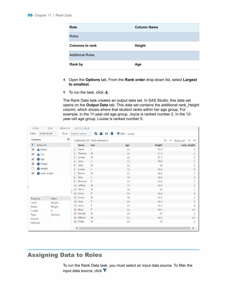
Role Column Name
Roles
Columns to rank Height
Additional Roles
Rank by Age
4 Open the Options tab. From the Rank order drop-down list, select Largest to smallest.
5 To run the task, click .
The Rank Data task creates an output data set. In SAS Studio, this data set opens on the Output Data tab. This data set contains the additional rank_Height column, which shows where that student ranks within her age group. For example, in the 11-year-old age group, Joyce is ranked number 2. In the 12-year-old age group, Louise is ranked number 5.
Assigning Data to Roles
To run the Rank Data task, you must select an input data source. To filter the input data source, click .
56 Chapter 11 / Rank Data
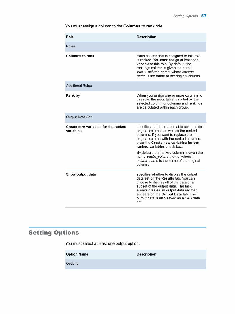
You must assign a column to the Columns to rank role.
Role Description
Roles
Columns to rank Each column that is assigned to this role is ranked. You must assign at least one variable to this role. By default, the rankings column is given the name rank_column-name, where column-name is the name of the original column.
Additional Roles
Rank by When you assign one or more columns to this role, the input table is sorted by the selected column or columns and rankings are calculated within each group.
Output Data Set
Create new variables for the ranked variables
specifies that the output table contains the original columns as well as the ranked columns. If you want to replace the original column with the ranked columns, clear the Create new variables for the ranked variables check box.
By default, the ranked column is given the name rank_column-name, where column-name is the name of the original column.
Show output data specifies whether to display the output data set on the Results tab. You can choose to display all of the data or a subset of the output data. The task always creates an output data set that appears on the Output Data tab. The output data is also saved as a SAS data set.
Setting Options
You must select at least one output option.
Option Name Description
Options
Setting Options 57
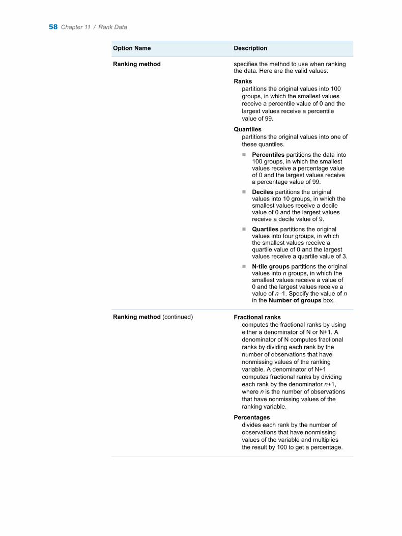
Option Name Description
Ranking method specifies the method to use when ranking the data. Here are the valid values:
Rankspartitions the original values into 100 groups, in which the smallest values receive a percentile value of 0 and the largest values receive a percentile value of 99.
Quantilespartitions the original values into one of these quantiles.
n Percentiles partitions the data into 100 groups, in which the smallest values receive a percentage value of 0 and the largest values receive a percentage value of 99.
n Deciles partitions the original values into 10 groups, in which the smallest values receive a decile value of 0 and the largest values receive a decile value of 9.
n Quartiles partitions the original values into four groups, in which the smallest values receive a quartile value of 0 and the largest values receive a quartile value of 3.
n N-tile groups partitions the original values into n groups, in which the smallest values receive a value of 0 and the largest values receive a value of n–1. Specify the value of n in the Number of groups box.
Ranking method (continued) Fractional rankscomputes the fractional ranks by using either a denominator of N or N+1. A denominator of N computes fractional ranks by dividing each rank by the number of observations that have nonmissing values of the ranking variable. A denominator of N+1 computes fractional ranks by dividing each rank by the denominator n+1, where n is the number of observations that have nonmissing values of the ranking variable.
Percentagesdivides each rank by the number of observations that have nonmissing values of the variable and multiplies the result by 100 to get a percentage.
58 Chapter 11 / Rank Data
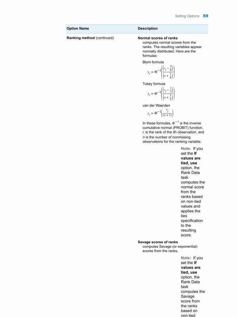
Option Name Description
Ranking method (continued) Normal scores of rankscomputes normal scores from the ranks. The resulting variables appear normally distributed. Here are the formulas:
Blom formula
yi = Φ−1 ri − 38
n + 14
Tukey formula
yi = Φ−1 ri − 13
n + 13
van der Waerden
yi = Φ−1 rin + 1
In these formulas, Φ−1 is the inverse cumulative normal (PROBIT) function, ri is the rank of the ith observation, and n is the number of nonmissing observations for the ranking variable.
Note: If you set the If values are tied, use option, the Rank Data task computes the normal score from the ranks based on non-tied values and applies the ties specification to the resulting score.
Savage scores of rankscomputes Savage (or exponential) scores from the ranks.
Note: If you set the If values are tied, use option, the Rank Data task computes the Savage score from the ranks based on non-tied values and applies the ties specification to the resulting score.
Setting Options 59
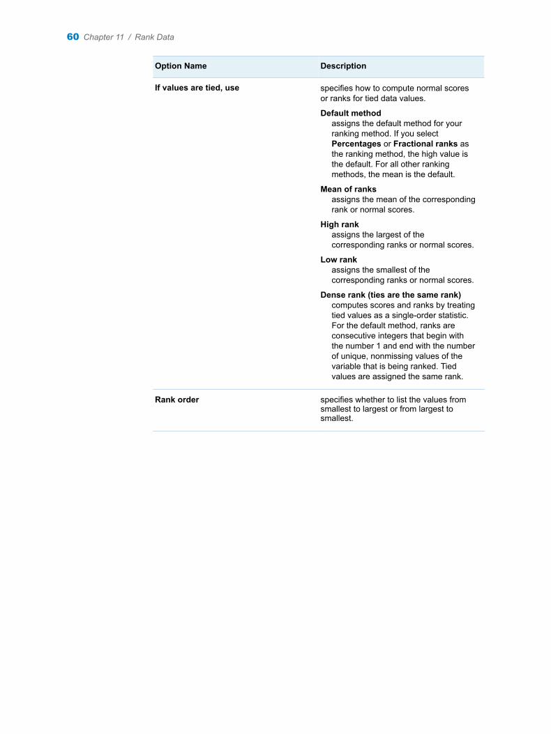
Option Name Description
If values are tied, use specifies how to compute normal scores or ranks for tied data values.
Default methodassigns the default method for your ranking method. If you select Percentages or Fractional ranks as the ranking method, the high value is the default. For all other ranking methods, the mean is the default.
Mean of ranksassigns the mean of the corresponding rank or normal scores.
High rankassigns the largest of the corresponding ranks or normal scores.
Low rankassigns the smallest of the corresponding ranks or normal scores.
Dense rank (ties are the same rank)computes scores and ranks by treating tied values as a single-order statistic. For the default method, ranks are consecutive integers that begin with the number 1 and end with the number of unique, nonmissing values of the variable that is being ranked. Tied values are assigned the same rank.
Rank order specifies whether to list the values from smallest to largest or from largest to smallest.
60 Chapter 11 / Rank Data
12Transform Data
About the Transform Data Task . . . . . . . . . . . . . . . . . . . . . . . . . . . . . . . . . . . . . . . . . . . . . 61
Example: Transforming the Data in the BASEBALL Data Set . . . . . . . . . . . . . . . . 61
Transforming Columns from the Input Data Set . . . . . . . . . . . . . . . . . . . . . . . . . . . . . 63
About the Transform Data Task
The Transform Data task enables you to transform one or more variables in the input data set. These transformed variables are saved to an output data set.
Example: Transforming the Data in the BASEBALL Data Set
1 In the Tasks section, expand the Data folder, and then double-click Transform Data. The user interface for the Transform Data task opens.
2 On the Data tab, select SASHELP.BASEBALL as the input data set.
TIP If the data set is not available from the drop-down list, click . In
the Choose a Table window, expand the library that contains the data set that you want to use. Select the data set for the example and click OK. The selected data set should now appear in the drop-down list.
61
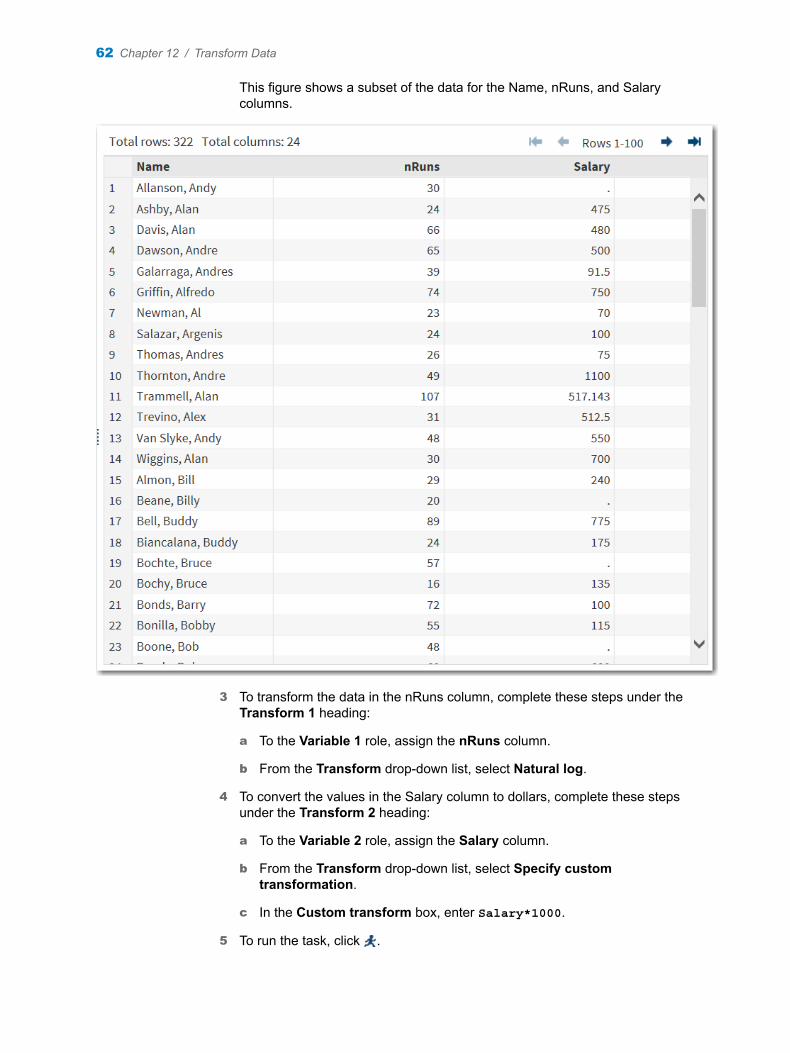
This figure shows a subset of the data for the Name, nRuns, and Salary columns.
3 To transform the data in the nRuns column, complete these steps under the Transform 1 heading:
a To the Variable 1 role, assign the nRuns column.
b From the Transform drop-down list, select Natural log.
4 To convert the values in the Salary column to dollars, complete these steps under the Transform 2 heading:
a To the Variable 2 role, assign the Salary column.
b From the Transform drop-down list, select Specify custom transformation.
c In the Custom transform box, enter Salary*1000.
5 To run the task, click .
62 Chapter 12 / Transform Data
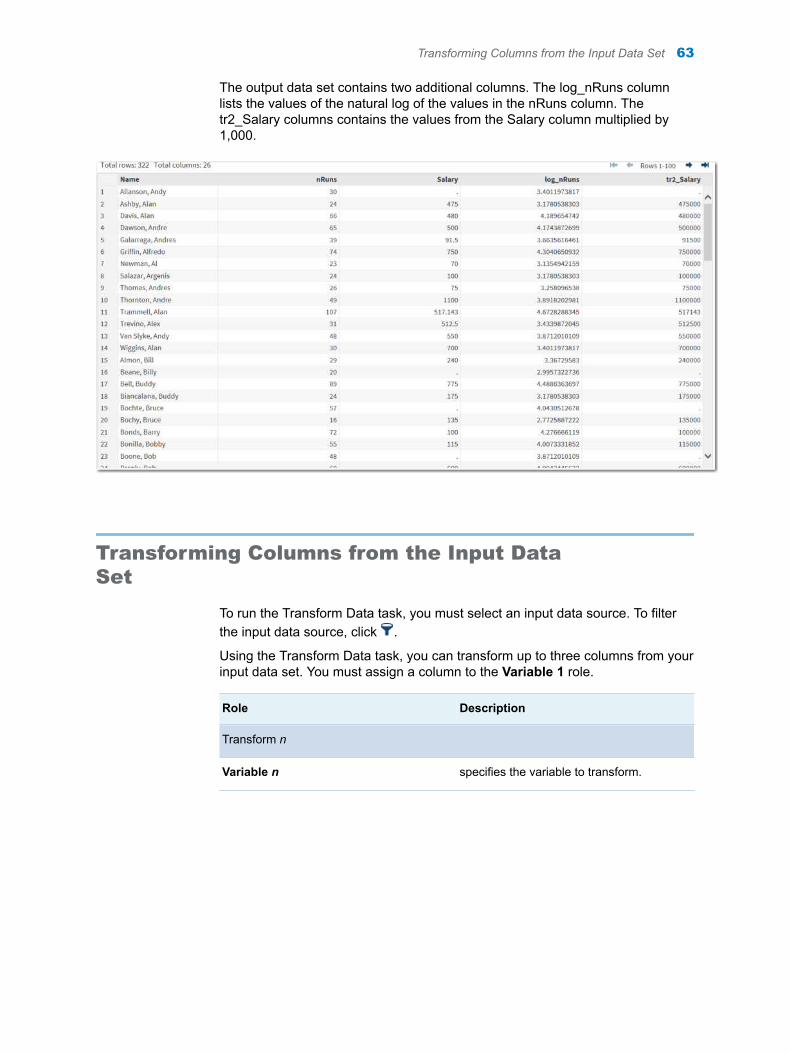
The output data set contains two additional columns. The log_nRuns column lists the values of the natural log of the values in the nRuns column. The tr2_Salary columns contains the values from the Salary column multiplied by 1,000.
Transforming Columns from the Input Data Set
To run the Transform Data task, you must select an input data source. To filter the input data source, click .
Using the Transform Data task, you can transform up to three columns from your input data set. You must assign a column to the Variable 1 role.
Role Description
Transform n
Variable n specifies the variable to transform.
Transforming Columns from the Input Data Set 63
Role Description
Transform specifies the transform to use. Here are the available transforms:n Inverse squaren Inversen Inverse square rootn Natural logn Square rootn SquareTo create your own transformation, select Specify custom transformation. An example of a custom transformation is Salary*1000.
Output Data Set
Show output data specifies whether to display the output data set on the Results tab. You can choose to display all of the data or a subset of the output data. The task always creates an output data set that appears on the Output Data tab. The output data is also saved as a SAS data set.
64 Chapter 12 / Transform Data
13Standardize Data
About the Standardize Data Task . . . . . . . . . . . . . . . . . . . . . . . . . . . . . . . . . . . . . . . . . . . 65
Example: Standardizing Variables in the SASHELP.BASEBALL Data Set . . . . 65
Assigning Data to Roles . . . . . . . . . . . . . . . . . . . . . . . . . . . . . . . . . . . . . . . . . . . . . . . . . . . . 66
Setting the Options . . . . . . . . . . . . . . . . . . . . . . . . . . . . . . . . . . . . . . . . . . . . . . . . . . . . . . . . . 67
Setting the Output Options . . . . . . . . . . . . . . . . . . . . . . . . . . . . . . . . . . . . . . . . . . . . . . . . . 68
About the Standardize Data Task
The Standardize Data task enables you to center or standardize one or more numeric variables using a variety of methods. The standardized variables are saved in an output data set.
Example: Standardizing Variables in the SASHELP.BASEBALL Data Set
To create this example:
1 In the Tasks section, expand the Data folder, and then double-click Standardize Data. The user interface for the Standardize Data task opens.
2 On the Data tab, select the SASHELP.BASEBALL data set.
TIP If the data set is not available from the drop-down list, click . In
the Choose a Table window, expand the library that contains the data set that you want to use. Select the data set for the example and click OK. The selected data set should now appear in the drop-down list.
3 To the Variables to standardize role, assign the nHits column.
4 To run the task, click .
65
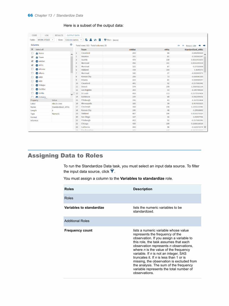
Here is a subset of the output data:
Assigning Data to Roles
To run the Standardize Data task, you must select an input data source. To filter the input data source, click .
You must assign a column to the Variables to standardize role.
Roles Description
Roles
Variables to standardize lists the numeric variables to be standardized.
Additional Roles
Frequency count lists a numeric variable whose value represents the frequency of the observation. If you assign a variable to this role, the task assumes that each observation represents n observations, where n is the value of the frequency variable. If n is not an integer, SAS truncates it. If n is less than 1 or is missing, the observation is excluded from the analysis. The sum of the frequency variable represents the total number of observations.
66 Chapter 13 / Standardize Data
Roles Description
Weight specifies a numeric variable in the input data set with values that are used to weight each observation. These values can be nonintegers. An observation is used in the analysis only if the value of the Weight variable is greater than zero.
Group analysis by enables you to obtain separate analyses of observations for each unique group.
Setting the Options
Option Name Description
Methods
Center data only specifies that you want to use either the mean or median standardization method.
Standardization method
specifies that you want to use one of these standardization methods:n Standard deviation (which is the default and the method
most often associated with standardization)n Andrew’s wave estimate. The tuning constant for this
method must be greater than 0. The default value is 4.7.n Euclidean lengthn Huber’s estimate. The tuning constant for this method must
be greater than 0. The default value is 1.n Interquartile rangen Maximum absolute valuen Median absolute deviationn Minkowskin Rangen Sumn Tukey’s biweight estimate. The tuning constant for this
method must be greater than 0. The default value is 6. (Goodall 1983)
n Art, Gnanadesikan, and Kettenring estimaten Minimum spacing
Treatment of Missing Values
Setting the Options 67
Option Name Description
Missing values method
specifies whether to omit observations with missing value or to replace the missing value. You can replace the missing values with one of these options:n Default location measure, which is the location measure
used by the selected centering or standardization methodn Meann Mediann Minimumn Specify custom value, which enables you to specify the
value for all variables that are being standardized
Statistics
Display location and scale measures
displays the location and scale measures in the results. These measures give you an idea of what the standardization process accomplished.
Setting the Output Options
By default, the Standardize Data task creates an output data set that includes both the original and standardized variables. You can add a prefix to the variable names to differentiate between the original and standardized variables. By default, the task adds the Standardize_ prefix to the standardized variable.
The Show output data option specifies whether to display the output data set on the Results tab. You can choose to display all of the data or a subset of the output data. The task always creates an output data set that appears on the Output Data tab. The output data is also saved as a SAS data set.
68 Chapter 13 / Standardize Data
Part 2
Graph Tasks
Chapter 14Bar Chart . . . . . . . . . . . . . . . . . . . . . . . . . . . . . . . . . . . . . . . . . . . . . . . . . . . . . . . . 71
Chapter 15Bar-Line Chart . . . . . . . . . . . . . . . . . . . . . . . . . . . . . . . . . . . . . . . . . . . . . . . . . . . 77
Chapter 16Box Plot . . . . . . . . . . . . . . . . . . . . . . . . . . . . . . . . . . . . . . . . . . . . . . . . . . . . . . . . . 83
Chapter 17Bubble Plot . . . . . . . . . . . . . . . . . . . . . . . . . . . . . . . . . . . . . . . . . . . . . . . . . . . . . . 87
Chapter 18Histogram . . . . . . . . . . . . . . . . . . . . . . . . . . . . . . . . . . . . . . . . . . . . . . . . . . . . . . . 91
Chapter 19Line Chart . . . . . . . . . . . . . . . . . . . . . . . . . . . . . . . . . . . . . . . . . . . . . . . . . . . . . . . 95
Chapter 20Mosaic Plot . . . . . . . . . . . . . . . . . . . . . . . . . . . . . . . . . . . . . . . . . . . . . . . . . . . . . . 99
Chapter 21Pie Chart . . . . . . . . . . . . . . . . . . . . . . . . . . . . . . . . . . . . . . . . . . . . . . . . . . . . . . . 103
Chapter 22Scatter Plot . . . . . . . . . . . . . . . . . . . . . . . . . . . . . . . . . . . . . . . . . . . . . . . . . . . . . 107
69

Chapter 23Series Plot . . . . . . . . . . . . . . . . . . . . . . . . . . . . . . . . . . . . . . . . . . . . . . . . . . . . . . 111
Chapter 24Simple HBar . . . . . . . . . . . . . . . . . . . . . . . . . . . . . . . . . . . . . . . . . . . . . . . . . . . . 115
70
14Bar Chart
About the Bar Chart Task . . . . . . . . . . . . . . . . . . . . . . . . . . . . . . . . . . . . . . . . . . . . . . . . . . . 71
Example: Bar Chart of Mean Sales for Each Product Line . . . . . . . . . . . . . . . . . . . 71
Assigning Data to Roles . . . . . . . . . . . . . . . . . . . . . . . . . . . . . . . . . . . . . . . . . . . . . . . . . . . . 72
Setting Options . . . . . . . . . . . . . . . . . . . . . . . . . . . . . . . . . . . . . . . . . . . . . . . . . . . . . . . . . . . . . 74
About the Bar Chart Task
The Bar Chart task creates horizontal or vertical bar charts that compare numeric values or statistics between different values of a chart variable. Bar charts show the relative magnitude of data by displaying bars of varying height. Each bar represents a category of data.
Example: Bar Chart of Mean Sales for Each Product Line
For example, you can create a bar chart that compares the total amount of sales for each product line in the Sashelp.Pricedata data set. By default, the task calculates the mean of the response variable for each product line. This bar chart shows that Line 2 has the highest mean product sales.
To create this example:
1 In the Tasks section, expand the Graph folder, and then double-click Bar Chart. The user interface for the Bar Chart task opens.
2 On the Data tab, select the SASHELP.PRICEDATA data set.
TIP If the data set is not available from the drop-down list, click . In
the Choose a Table window, expand the library that contains the data set that you want to use. Select the data set for the example and click OK. The selected data set should now appear in the drop-down list.
3 Assign columns to these roles:
71
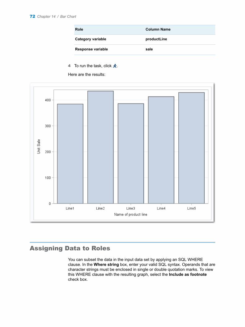
Role Column Name
Category variable productLine
Response variable sale
4 To run the task, click .
Here are the results:
Assigning Data to Roles
You can subset the data in the input data set by applying an SQL WHERE clause. In the Where string box, enter your valid SQL syntax. Operands that are character strings must be enclosed in single or double quotation marks. To view this WHERE clause with the resulting graph, select the Include as footnote check box.
72 Chapter 14 / Bar Chart
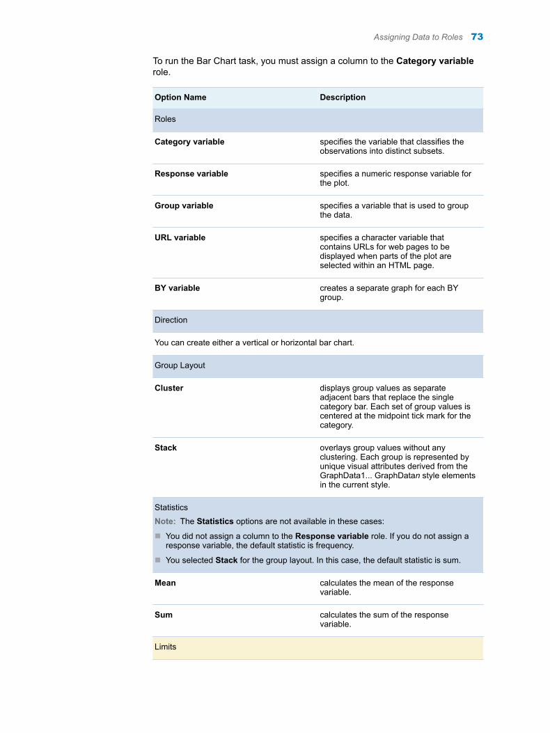
To run the Bar Chart task, you must assign a column to the Category variable role.
Option Name Description
Roles
Category variable specifies the variable that classifies the observations into distinct subsets.
Response variable specifies a numeric response variable for the plot.
Group variable specifies a variable that is used to group the data.
URL variable specifies a character variable that contains URLs for web pages to be displayed when parts of the plot are selected within an HTML page.
BY variable creates a separate graph for each BY group.
Direction
You can create either a vertical or horizontal bar chart.
Group Layout
Cluster displays group values as separate adjacent bars that replace the single category bar. Each set of group values is centered at the midpoint tick mark for the category.
Stack overlays group values without any clustering. Each group is represented by unique visual attributes derived from the GraphData1... GraphDatan style elements in the current style.
Statistics
Note: The Statistics options are not available in these cases:
n You did not assign a column to the Response variable role. If you do not assign a response variable, the default statistic is frequency.
n You selected Stack for the group layout. In this case, the default statistic is sum.
Mean calculates the mean of the response variable.
Sum calculates the sum of the response variable.
Limits
Assigning Data to Roles 73
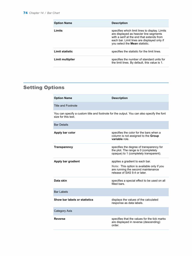
Option Name Description
Limits specifies which limit lines to display. Limits are displayed as heavier line segments with a serif at the end that extends from each bar. Limit lines are displayed only if you select the Mean statistic.
Limit statistic specifies the statistic for the limit lines.
Limit multiplier specifies the number of standard units for the limit lines. By default, this value is 1.
Setting Options
Option Name Description
Title and Footnote
You can specify a custom title and footnote for the output. You can also specify the font size for this text.
Bar Details
Apply bar color specifies the color for the bars when a column is not assigned to the Group variable role.
Transparency specifies the degree of transparency for the plot. The range is 0 (completely opaque) to 1 (completely transparent).
Apply bar gradient applies a gradient to each bar.
Note: This option is available only if you are running the second maintenance release of SAS 9.4 or later.
Data skin specifies a special effect to be used on all filled bars.
Bar Labels
Show bar labels or statistics displays the values of the calculated response as data labels.
Category Axis
Reverse specifies that the values for the tick marks are displayed in reverse (descending) order.
74 Chapter 14 / Bar Chart
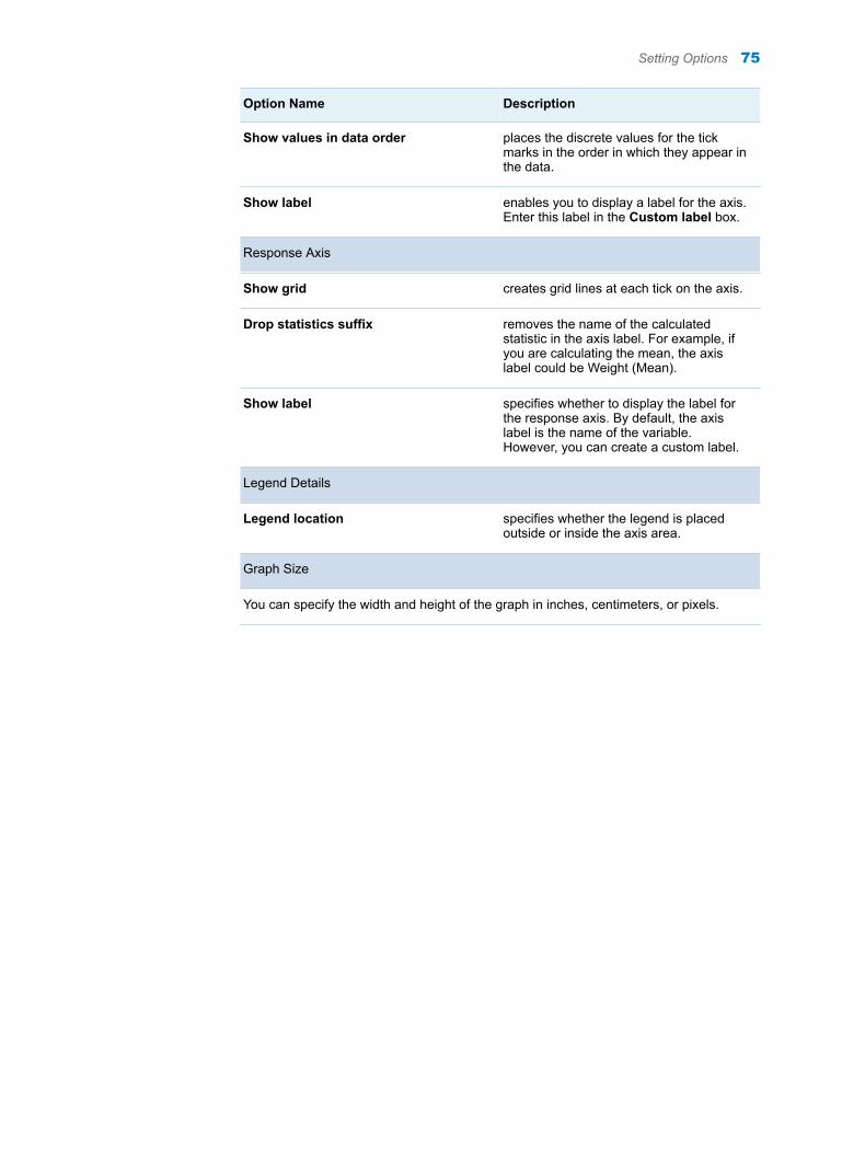
Option Name Description
Show values in data order places the discrete values for the tick marks in the order in which they appear in the data.
Show label enables you to display a label for the axis. Enter this label in the Custom label box.
Response Axis
Show grid creates grid lines at each tick on the axis.
Drop statistics suffix removes the name of the calculated statistic in the axis label. For example, if you are calculating the mean, the axis label could be Weight (Mean).
Show label specifies whether to display the label for the response axis. By default, the axis label is the name of the variable. However, you can create a custom label.
Legend Details
Legend location specifies whether the legend is placed outside or inside the axis area.
Graph Size
You can specify the width and height of the graph in inches, centimeters, or pixels.
Setting Options 75

76 Chapter 14 / Bar Chart
15Bar-Line Chart
About the Bar-Line Chart Task . . . . . . . . . . . . . . . . . . . . . . . . . . . . . . . . . . . . . . . . . . . . . . 77
Example: City and Highway Mileage by Origin . . . . . . . . . . . . . . . . . . . . . . . . . . . . . . 77
Assigning Data to Roles . . . . . . . . . . . . . . . . . . . . . . . . . . . . . . . . . . . . . . . . . . . . . . . . . . . . 78
Setting Options . . . . . . . . . . . . . . . . . . . . . . . . . . . . . . . . . . . . . . . . . . . . . . . . . . . . . . . . . . . . . 79
About the Bar-Line Chart Task
The Bar-Line Chart task creates a vertical bar chart with a line chart overlay.
You can use this task to perform the following tasks:
n display and compare exact and relative magnitudes
n examine the contribution of each part to the whole
n determine trends and patterns in the data
Example: City and Highway Mileage by Origin
For example, you can create a bar-line chart that compares the number of miles per gallon (in the city and on the highway) that cars use depending on their country of origin. The task calculates the mean of the number of miles per gallon in the city and in the highway for each country. This bar-line chart shows that cars from Asia tend to get the highest number of miles per gallon in city and highway driving.
To create this example:
1 In the Tasks section, expand the Graph folder, and then double-click Bar-Line Chart. The user interface for the Bar-Line Chart task opens.
2 On the Data tab, select the SASHELP.CARS data set.
TIP If the data set is not available from the drop-down list, click . In
the Choose a Table window, expand the library that contains the data set
77
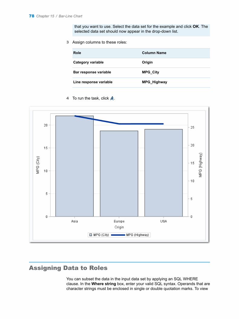
that you want to use. Select the data set for the example and click OK. The selected data set should now appear in the drop-down list.
3 Assign columns to these roles:
Role Column Name
Category variable Origin
Bar response variable MPG_City
Line response variable MPG_Highway
4 To run the task, click .
Assigning Data to Roles
You can subset the data in the input data set by applying an SQL WHERE clause. In the Where string box, enter your valid SQL syntax. Operands that are character strings must be enclosed in single or double quotation marks. To view
78 Chapter 15 / Bar-Line Chart

this WHERE clause with the resulting graph, select the Include as footnote check box.
To run the Bar-Line Chart task, you must assign a column to the Category variable, Bar response variable, and Line response variable roles.
Option Name Description
Roles
Category variable specifies the variable that classifies the observations into distinct subsets.
Bar response variable specifies a numeric response variable for the bar chart.
Line response variable specifies a numeric response variable for the line plot.
Group variable specifies a variable that is used to group the data.
URL variable specifies a character variable that contains URLs for web pages to be displayed when parts of the plot are selected within an HTML page.
Statistics
Mean calculates the mean of the response variables.
Sum calculates the sum of the response variables.
Setting Options
Option Name Description
Title and Footnote
You can specify a custom title and footnote for the output. You can also specify the font size for this text.
Bar Details
Apply bar color specifies the color for the bars.
Transparency specifies the degree of transparency for the plot. The range is 0 (completely opaque) to 1 (completely transparent).
Setting Options 79
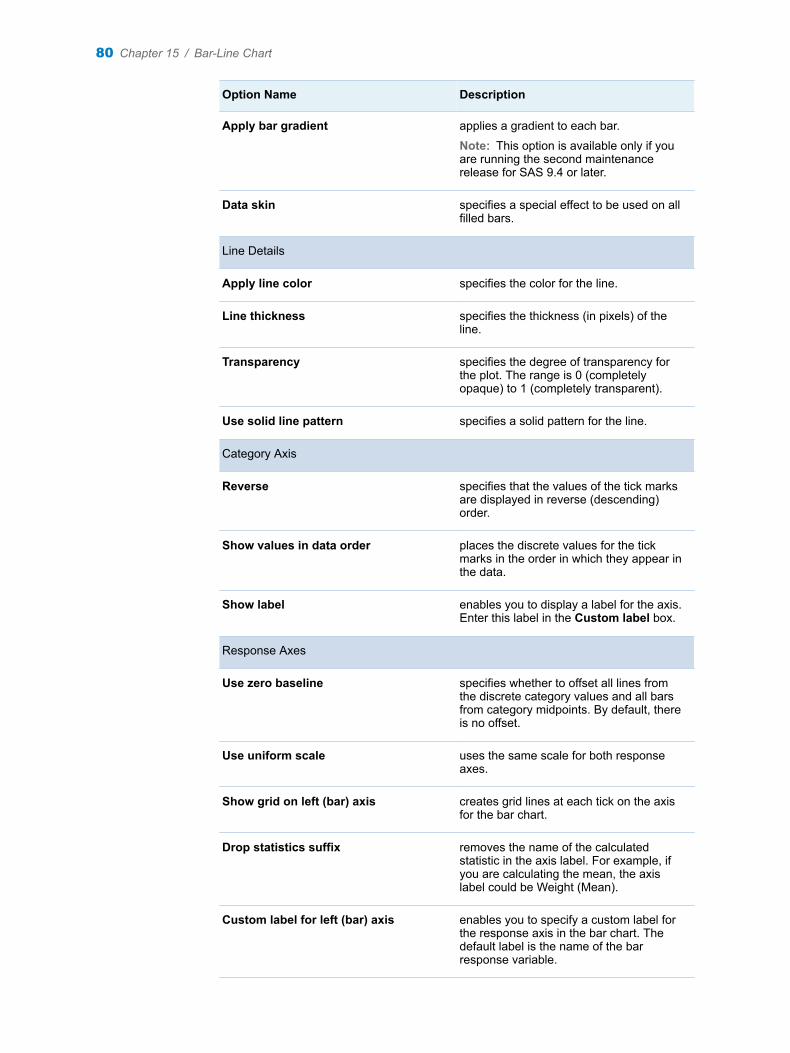
Option Name Description
Apply bar gradient applies a gradient to each bar.
Note: This option is available only if you are running the second maintenance release for SAS 9.4 or later.
Data skin specifies a special effect to be used on all filled bars.
Line Details
Apply line color specifies the color for the line.
Line thickness specifies the thickness (in pixels) of the line.
Transparency specifies the degree of transparency for the plot. The range is 0 (completely opaque) to 1 (completely transparent).
Use solid line pattern specifies a solid pattern for the line.
Category Axis
Reverse specifies that the values of the tick marks are displayed in reverse (descending) order.
Show values in data order places the discrete values for the tick marks in the order in which they appear in the data.
Show label enables you to display a label for the axis. Enter this label in the Custom label box.
Response Axes
Use zero baseline specifies whether to offset all lines from the discrete category values and all bars from category midpoints. By default, there is no offset.
Use uniform scale uses the same scale for both response axes.
Show grid on left (bar) axis creates grid lines at each tick on the axis for the bar chart.
Drop statistics suffix removes the name of the calculated statistic in the axis label. For example, if you are calculating the mean, the axis label could be Weight (Mean).
Custom label for left (bar) axis enables you to specify a custom label for the response axis in the bar chart. The default label is the name of the bar response variable.
80 Chapter 15 / Bar-Line Chart
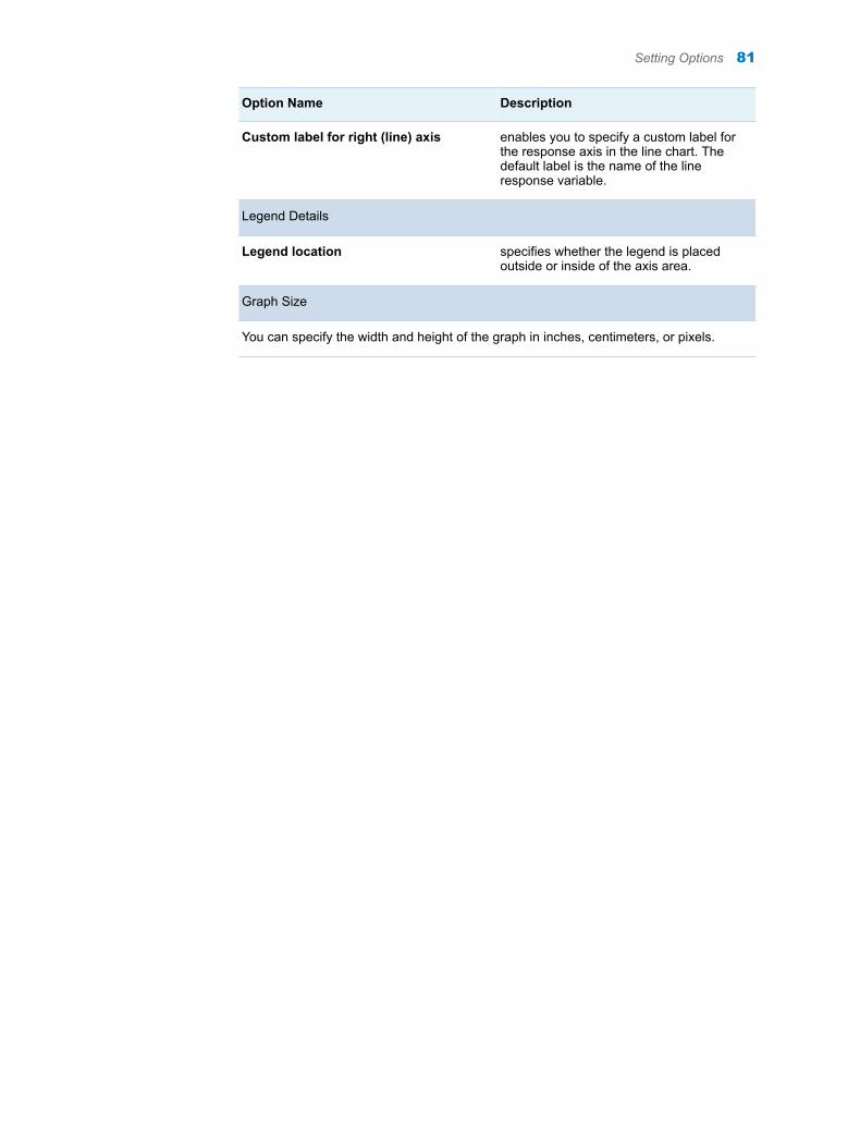
Option Name Description
Custom label for right (line) axis enables you to specify a custom label for the response axis in the line chart. The default label is the name of the line response variable.
Legend Details
Legend location specifies whether the legend is placed outside or inside of the axis area.
Graph Size
You can specify the width and height of the graph in inches, centimeters, or pixels.
Setting Options 81

82 Chapter 15 / Bar-Line Chart

16Box Plot
About the Box Plot Task . . . . . . . . . . . . . . . . . . . . . . . . . . . . . . . . . . . . . . . . . . . . . . . . . . . . 83
Example: Box Plots Comparing MPG (City) for Cars . . . . . . . . . . . . . . . . . . . . . . . . . 83
Assigning Data to Roles . . . . . . . . . . . . . . . . . . . . . . . . . . . . . . . . . . . . . . . . . . . . . . . . . . . . 84
Setting Options . . . . . . . . . . . . . . . . . . . . . . . . . . . . . . . . . . . . . . . . . . . . . . . . . . . . . . . . . . . . . 85
About the Box Plot Task
The Box Plot task creates a single box plot, which represents numeric values measured as intervals. If you choose to categorize the values of the analysis variable, then multiple box plots are created.
Example: Box Plots Comparing MPG (City) for Cars
This example creates three box plots that compares how many miles per gallon (city) cars consume depending on their area of origin (Asia, Europe, and United States).
To create this example:
1 In the Tasks section, expand the Graph folder, and then double-click Box Plot. The user interface for the Box Plot task opens.
2 On the Data tab, select the SASHELP.CARS data set.
TIP If the data set is not available from the drop-down list, click . In
the Choose a Table window, expand the library that contains the data set that you want to use. Select the data set for the example and click OK. The selected data set should now appear in the drop-down list.
3 Assign columns to these roles:
83
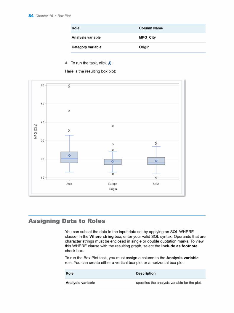
Role Column Name
Analysis variable MPG_City
Category variable Origin
4 To run the task, click .
Here is the resulting box plot:
Assigning Data to Roles
You can subset the data in the input data set by applying an SQL WHERE clause. In the Where string box, enter your valid SQL syntax. Operands that are character strings must be enclosed in single or double quotation marks. To view this WHERE clause with the resulting graph, select the Include as footnote check box.
To run the Box Plot task, you must assign a column to the Analysis variable role. You can create either a vertical box plot or a horizontal box plot.
Role Description
Analysis variable specifies the analysis variable for the plot.
84 Chapter 16 / Box Plot
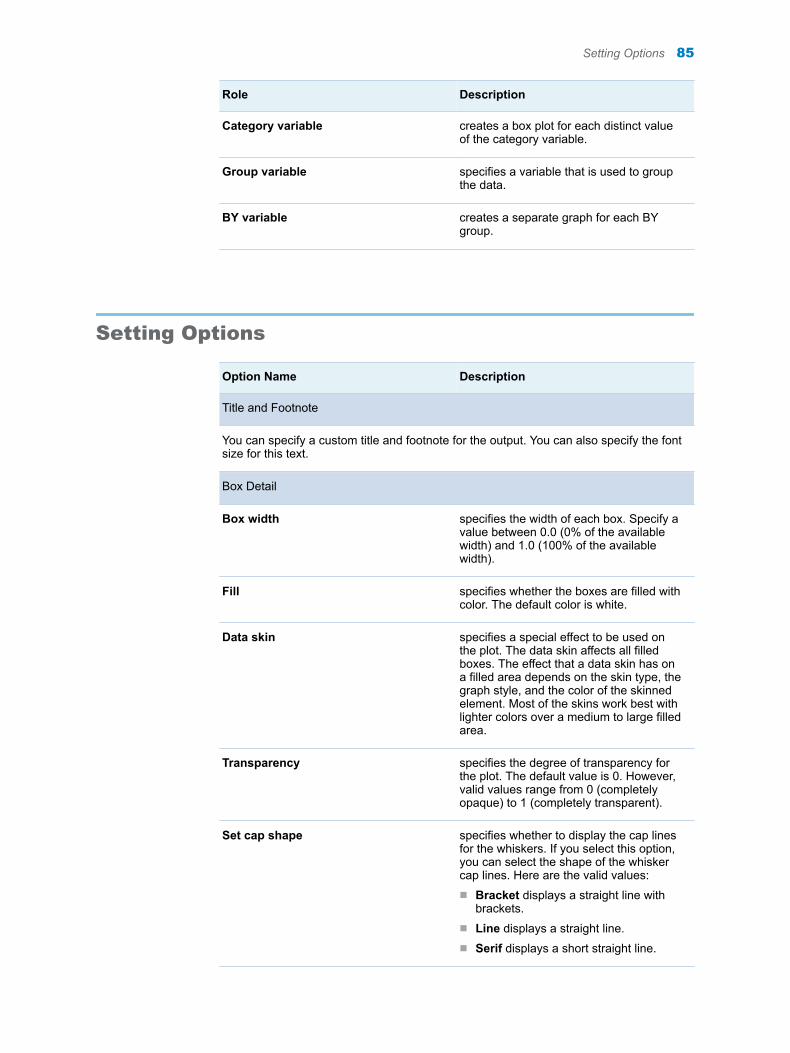
Role Description
Category variable creates a box plot for each distinct value of the category variable.
Group variable specifies a variable that is used to group the data.
BY variable creates a separate graph for each BY group.
Setting Options
Option Name Description
Title and Footnote
You can specify a custom title and footnote for the output. You can also specify the font size for this text.
Box Detail
Box width specifies the width of each box. Specify a value between 0.0 (0% of the available width) and 1.0 (100% of the available width).
Fill specifies whether the boxes are filled with color. The default color is white.
Data skin specifies a special effect to be used on the plot. The data skin affects all filled boxes. The effect that a data skin has on a filled area depends on the skin type, the graph style, and the color of the skinned element. Most of the skins work best with lighter colors over a medium to large filled area.
Transparency specifies the degree of transparency for the plot. The default value is 0. However, valid values range from 0 (completely opaque) to 1 (completely transparent).
Set cap shape specifies whether to display the cap lines for the whiskers. If you select this option, you can select the shape of the whisker cap lines. Here are the valid values:n Bracket displays a straight line with
brackets.n Line displays a straight line.n Serif displays a short straight line.
Setting Options 85
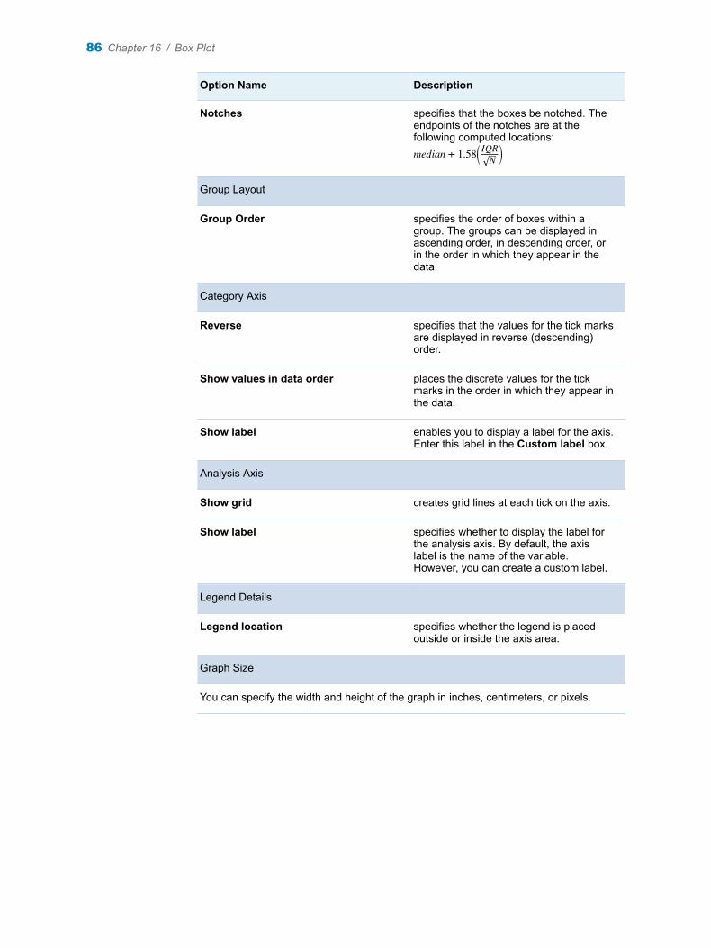
Option Name Description
Notches specifies that the boxes be notched. The endpoints of the notches are at the following computed locations: median ± 1.58 IQR
N
Group Layout
Group Order specifies the order of boxes within a group. The groups can be displayed in ascending order, in descending order, or in the order in which they appear in the data.
Category Axis
Reverse specifies that the values for the tick marks are displayed in reverse (descending) order.
Show values in data order places the discrete values for the tick marks in the order in which they appear in the data.
Show label enables you to display a label for the axis. Enter this label in the Custom label box.
Analysis Axis
Show grid creates grid lines at each tick on the axis.
Show label specifies whether to display the label for the analysis axis. By default, the axis label is the name of the variable. However, you can create a custom label.
Legend Details
Legend location specifies whether the legend is placed outside or inside the axis area.
Graph Size
You can specify the width and height of the graph in inches, centimeters, or pixels.
86 Chapter 16 / Box Plot
17Bubble Plot
About the Bubble Plot Task . . . . . . . . . . . . . . . . . . . . . . . . . . . . . . . . . . . . . . . . . . . . . . . . . 87
Example: Bubble Plot . . . . . . . . . . . . . . . . . . . . . . . . . . . . . . . . . . . . . . . . . . . . . . . . . . . . . . . 87
Assigning Data to Roles . . . . . . . . . . . . . . . . . . . . . . . . . . . . . . . . . . . . . . . . . . . . . . . . . . . . 88
Setting Options . . . . . . . . . . . . . . . . . . . . . . . . . . . . . . . . . . . . . . . . . . . . . . . . . . . . . . . . . . . . . 89
About the Bubble Plot Task
The Bubble Plot task explores the relationship between three or more variables. In a bubble plot, two variables determine the location of the bubble centers, and a third variable specifies the size of each bubble.
Example: Bubble Plot
To create this example:
1 In the Tasks section, expand the Graph folder, and then double-click Bubble Plot. The user interface for the Bubble Plot task opens.
2 On the Data tab, select the SASHELP.CLASS data set.
TIP If the data set is not available from the drop-down list, click . In
the Choose a Table window, expand the library that contains the data set that you want to use. Select the data set for the example and click OK. The selected data set should now appear in the drop-down list.
3 Assign columns to these roles:
Role Column Name
X variable Height
Y variable Weight
87
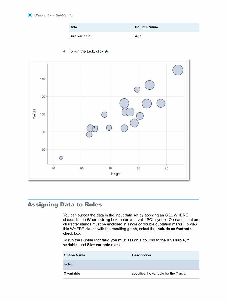
Role Column Name
Size variable Age
4 To run the task, click .
Assigning Data to Roles
You can subset the data in the input data set by applying an SQL WHERE clause. In the Where string box, enter your valid SQL syntax. Operands that are character strings must be enclosed in single or double quotation marks. To view this WHERE clause with the resulting graph, select the Include as footnote check box.
To run the Bubble Plot task, you must assign a column to the X variable, Y variable, and Size variable roles.
Option Name Description
Roles
X variable specifies the variable for the X axis.
88 Chapter 17 / Bubble Plot
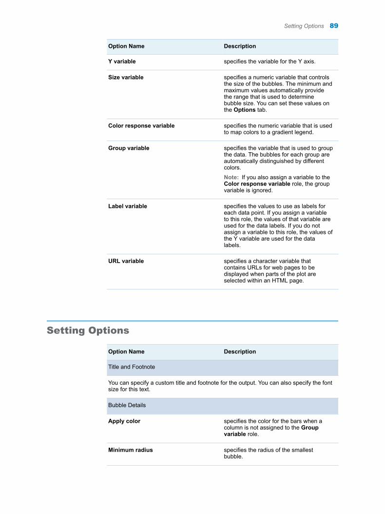
Option Name Description
Y variable specifies the variable for the Y axis.
Size variable specifies a numeric variable that controls the size of the bubbles. The minimum and maximum values automatically provide the range that is used to determine bubble size. You can set these values on the Options tab.
Color response variable specifies the numeric variable that is used to map colors to a gradient legend.
Group variable specifies the variable that is used to group the data. The bubbles for each group are automatically distinguished by different colors.
Note: If you also assign a variable to the Color response variable role, the group variable is ignored.
Label variable specifies the values to use as labels for each data point. If you assign a variable to this role, the values of that variable are used for the data labels. If you do not assign a variable to this role, the values of the Y variable are used for the data labels.
URL variable specifies a character variable that contains URLs for web pages to be displayed when parts of the plot are selected within an HTML page.
Setting Options
Option Name Description
Title and Footnote
You can specify a custom title and footnote for the output. You can also specify the font size for this text.
Bubble Details
Apply color specifies the color for the bars when a column is not assigned to the Group variable role.
Minimum radius specifies the radius of the smallest bubble.
Setting Options 89
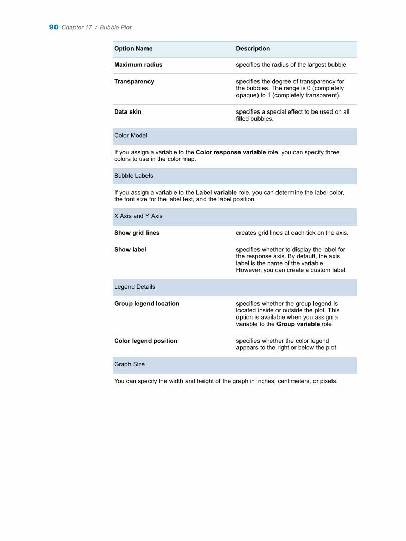
Option Name Description
Maximum radius specifies the radius of the largest bubble.
Transparency specifies the degree of transparency for the bubbles. The range is 0 (completely opaque) to 1 (completely transparent).
Data skin specifies a special effect to be used on all filled bubbles.
Color Model
If you assign a variable to the Color response variable role, you can specify three colors to use in the color map.
Bubble Labels
If you assign a variable to the Label variable role, you can determine the label color, the font size for the label text, and the label position.
X Axis and Y Axis
Show grid lines creates grid lines at each tick on the axis.
Show label specifies whether to display the label for the response axis. By default, the axis label is the name of the variable. However, you can create a custom label.
Legend Details
Group legend location specifies whether the group legend is located inside or outside the plot. This option is available when you assign a variable to the Group variable role.
Color legend position specifies whether the color legend appears to the right or below the plot.
Graph Size
You can specify the width and height of the graph in inches, centimeters, or pixels.
90 Chapter 17 / Bubble Plot
18Histogram
About the Histogram Task . . . . . . . . . . . . . . . . . . . . . . . . . . . . . . . . . . . . . . . . . . . . . . . . . . 91
Example: Histogram of Stock Volume . . . . . . . . . . . . . . . . . . . . . . . . . . . . . . . . . . . . . . . 91
Assigning Data to Roles . . . . . . . . . . . . . . . . . . . . . . . . . . . . . . . . . . . . . . . . . . . . . . . . . . . . 92
Setting Options . . . . . . . . . . . . . . . . . . . . . . . . . . . . . . . . . . . . . . . . . . . . . . . . . . . . . . . . . . . . . 92
About the Histogram Task
The Histograms task creates a chart that displays the frequency distribution of a numeric variable.
Example: Histogram of Stock Volume
To create this example:
1 In the Tasks section, expand the Graph folder, and then double-click Histogram. The user interface for the Histogram task opens.
2 In the Data tab, select the SASHELP.STOCKS data set.
TIP If the data set is not available from the drop-down list, click . In
the Choose a Table window, expand the library that contains the data set that you want to use. Select the data set for the example and click OK. The selected data set should now appear in the drop-down list.
3 To the Analysis variable role, assign the Volume column.
4 To run the task, click .
91
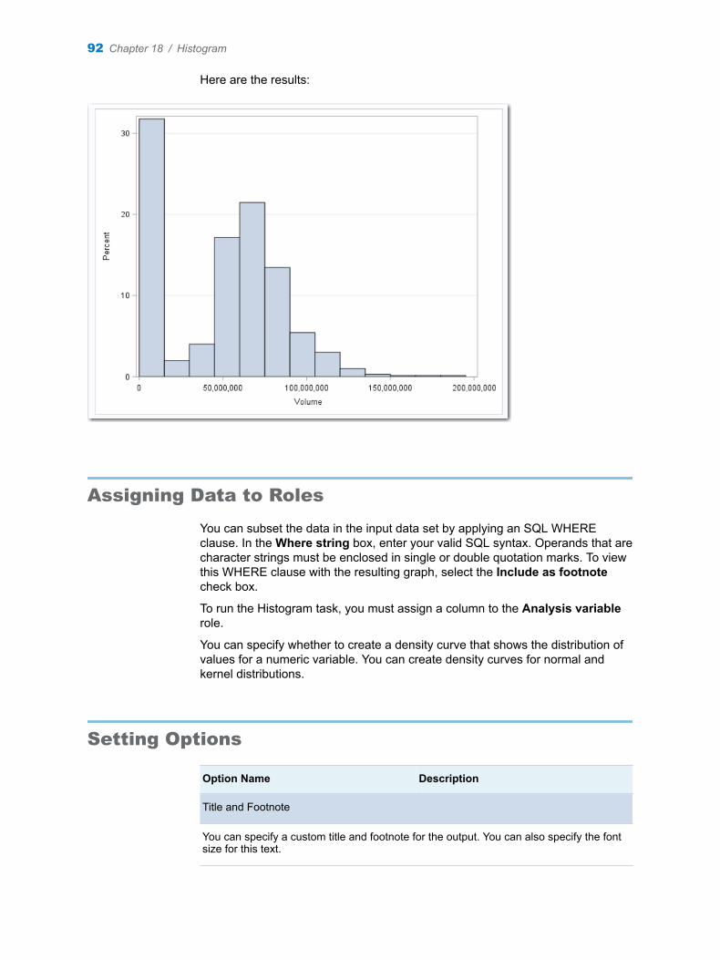
Here are the results:
Assigning Data to Roles
You can subset the data in the input data set by applying an SQL WHERE clause. In the Where string box, enter your valid SQL syntax. Operands that are character strings must be enclosed in single or double quotation marks. To view this WHERE clause with the resulting graph, select the Include as footnote check box.
To run the Histogram task, you must assign a column to the Analysis variable role.
You can specify whether to create a density curve that shows the distribution of values for a numeric variable. You can create density curves for normal and kernel distributions.
Setting Options
Option Name Description
Title and Footnote
You can specify a custom title and footnote for the output. You can also specify the font size for this text.
92 Chapter 18 / Histogram
Option Name Description
Bin Details
For the bins in the histogram, you can specify the color and the transparency. If you are running the second maintenance release for SAS 9.4 or later, you can also specify whether to apply a gradient to each bin.
Horizontal Axis
Interval axis creates tick marks at regular intervals on the horizontal axis based on the minimum and maximum values of the analysis variable.
Bin axis creates tick marks at the midpoints of the value bins on the horizontal axis.
Specify number of bins enables you to specify the number of bins in the histogram. Valid values range from 2 to 20.
The bins always span the range of data. The task tries to produce tick values that are easily interpreted (for example, 5, 10, 15, 20). Sometimes the location of the first bin and the bin width might be adjusted. By default, the task automatically determines the number of bins.
Show label displays the label for the analysis variable along the horizontal axis. You can also enter a custom label.
Vertical Axis
Specify axis scaling specifies the scaling that is applied to the vertical axis. You can choose from these options:
COUNTthe axis displays the frequency count
PERCENTthe axis displays values as a percentage of the total.
PROPORTIONthe axis displays values as proportions (0.0 to 1.0) of the total.
Show grid specifies whether to show the grid lines for the vertical axis.
Show label specifies whether to show the label for the type of axis scaling.
Legend Details
Setting Options 93
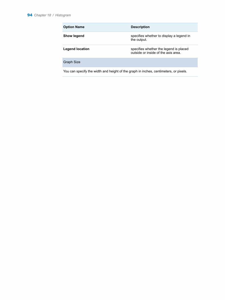
Option Name Description
Show legend specifies whether to display a legend in the output.
Legend location specifies whether the legend is placed outside or inside of the axis area.
Graph Size
You can specify the width and height of the graph in inches, centimeters, or pixels.
94 Chapter 18 / Histogram
19Line Chart
About the Line Chart Task . . . . . . . . . . . . . . . . . . . . . . . . . . . . . . . . . . . . . . . . . . . . . . . . . . 95
Example: Displaying the Mean Horsepower for Each Car Type . . . . . . . . . . . . . . 95
Assigning Data to Roles . . . . . . . . . . . . . . . . . . . . . . . . . . . . . . . . . . . . . . . . . . . . . . . . . . . . 96
Setting Options . . . . . . . . . . . . . . . . . . . . . . . . . . . . . . . . . . . . . . . . . . . . . . . . . . . . . . . . . . . . . 97
About the Line Chart Task
The Line Chart task assumes that the values in the category variable are discrete. The task groups these values into distinct categories. If you assign a column from the input data source to the Response variable role, you can select the statistic (either mean or sum) for the response values. By default, the task calculates the mean of the values for the response variable. If no response variable is assigned, a frequency chart by category is created.
Example: Displaying the Mean Horsepower for Each Car Type
In this example, you want to display the mean horsepower for each car type in a line plot. The result shows that sports cars have the highest average horsepower and hybrid cars have the lowest average horsepower.
To create this example:
1 In the Tasks section, expand the Graph folder, and then double-click Line Chart. The user interface for the Line Chart task opens.
2 On the Data tab, select the SASHELP.CARS data set.
TIP If the data set is not available from the drop-down list, click . In
the Choose a Table window, expand the library that contains the data set that you want to use. Select the data set for the example and click OK. The selected data set should now appear in the drop-down list.
3 Assign columns to these roles:
95
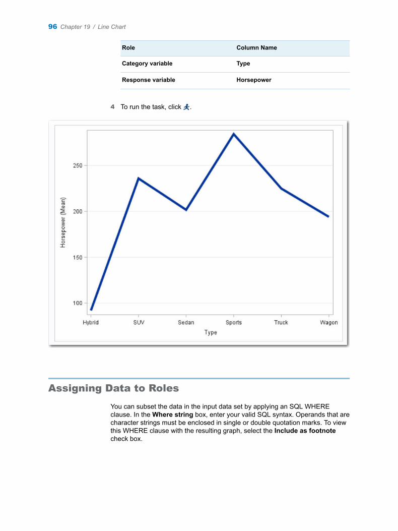
Role Column Name
Category variable Type
Response variable Horsepower
4 To run the task, click .
Assigning Data to Roles
You can subset the data in the input data set by applying an SQL WHERE clause. In the Where string box, enter your valid SQL syntax. Operands that are character strings must be enclosed in single or double quotation marks. To view this WHERE clause with the resulting graph, select the Include as footnote check box.
96 Chapter 19 / Line Chart
To run the Line Chart task, you must assign a column to the Category variable role.
Option Name Description
Role
Category variable specifies the variable that classifies the observations into distinct subsets.
Response variable specifies a numeric response variable for the plot.
Group variable specifies a variable that is used to group the data.
URL variable specifies a character variable that contains URLs for web pages to be displayed when parts of the plot are selected within an HTML page.
Statistics
Mean calculates the mean of the response variable.
Sum calculates the sum of the response variable.
Setting Options
Option Name Description
Title and Footnote
You can specify a custom title and footnote for the output. You can also specify the font size for this text.
Line Details
Apply line color specifies the color for the line when you do not assign a column to the Group variable role.
Line thickness specifies the thickness (in pixels) of the line.
Transparency specifies the degree of transparency for the plot. The range is 0 (completely opaque) to 1 (completely transparent).
Use solid line specifies a solid pattern for the line.
Setting Options 97
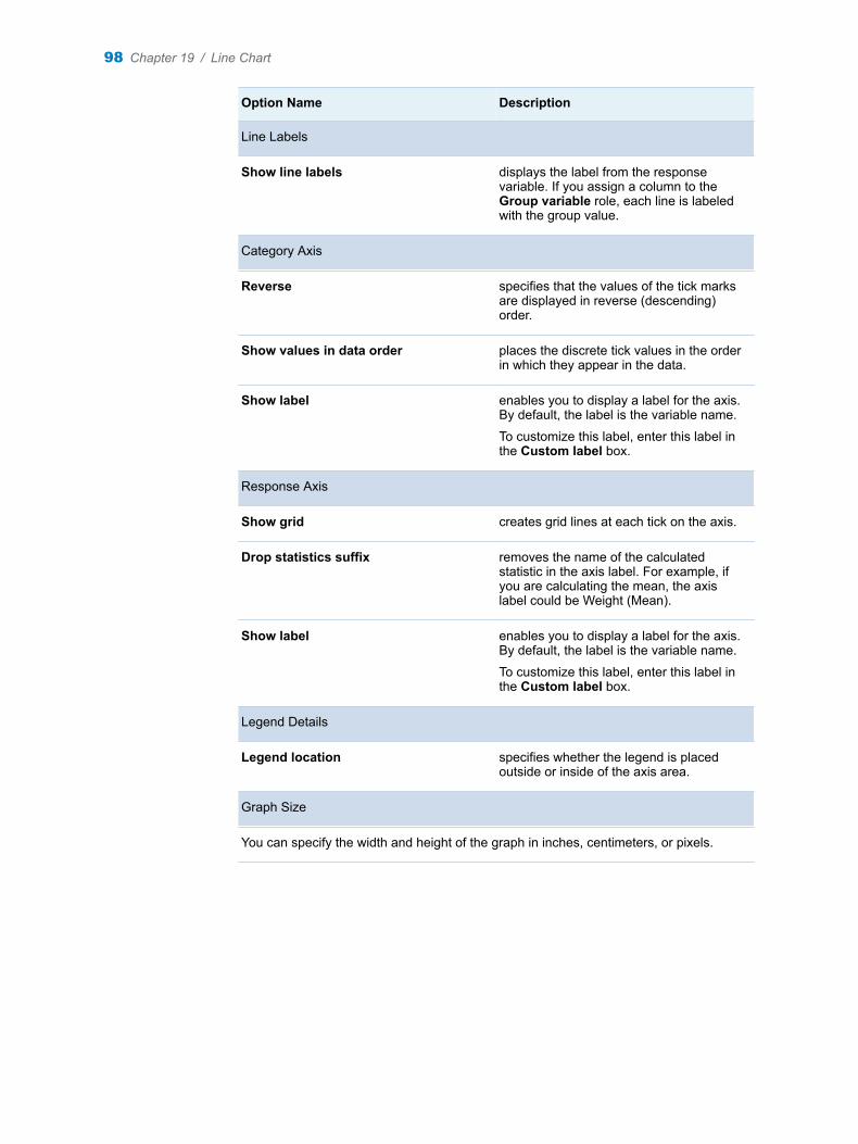
Option Name Description
Line Labels
Show line labels displays the label from the response variable. If you assign a column to the Group variable role, each line is labeled with the group value.
Category Axis
Reverse specifies that the values of the tick marks are displayed in reverse (descending) order.
Show values in data order places the discrete tick values in the order in which they appear in the data.
Show label enables you to display a label for the axis. By default, the label is the variable name.
To customize this label, enter this label in the Custom label box.
Response Axis
Show grid creates grid lines at each tick on the axis.
Drop statistics suffix removes the name of the calculated statistic in the axis label. For example, if you are calculating the mean, the axis label could be Weight (Mean).
Show label enables you to display a label for the axis. By default, the label is the variable name.
To customize this label, enter this label in the Custom label box.
Legend Details
Legend location specifies whether the legend is placed outside or inside of the axis area.
Graph Size
You can specify the width and height of the graph in inches, centimeters, or pixels.
98 Chapter 19 / Line Chart

20Mosaic Plot
About the Mosaic Plot Task . . . . . . . . . . . . . . . . . . . . . . . . . . . . . . . . . . . . . . . . . . . . . . . . . 99
Example: Mosaic Plot . . . . . . . . . . . . . . . . . . . . . . . . . . . . . . . . . . . . . . . . . . . . . . . . . . . . . . . 99
Assigning Data to Roles . . . . . . . . . . . . . . . . . . . . . . . . . . . . . . . . . . . . . . . . . . . . . . . . . . . 100
Setting Options . . . . . . . . . . . . . . . . . . . . . . . . . . . . . . . . . . . . . . . . . . . . . . . . . . . . . . . . . . . . 101
About the Mosaic Plot Task
Mosaic plots display tiles that correspond to the crosstabulation table cells. The areas of the tiles are proportional to the frequencies of the table cells. The column variable is displayed on the X axis, and the tile widths are proportional to the relative frequencies of the column variable levels. The row variable is displayed on the Y axis, and the tile heights are proportional to the relative frequencies of the row levels within column levels. For more information, see Friendly (2000).
Example: Mosaic Plot
To create this example:
1 In the Tasks section, expand the Graph folder, and then double-click Mosaic. The user interface for the Mosaic Plot task opens.
2 On the Data tab, select the SASHELP.CARS data set.
TIP If the data set is not available from the drop-down list, click . In
the Choose a Table window, expand the library that contains the data set that you want to use. Select the data set for the example and click OK. The selected data set should now appear in the drop-down list.
3 Assign columns to these roles:
99
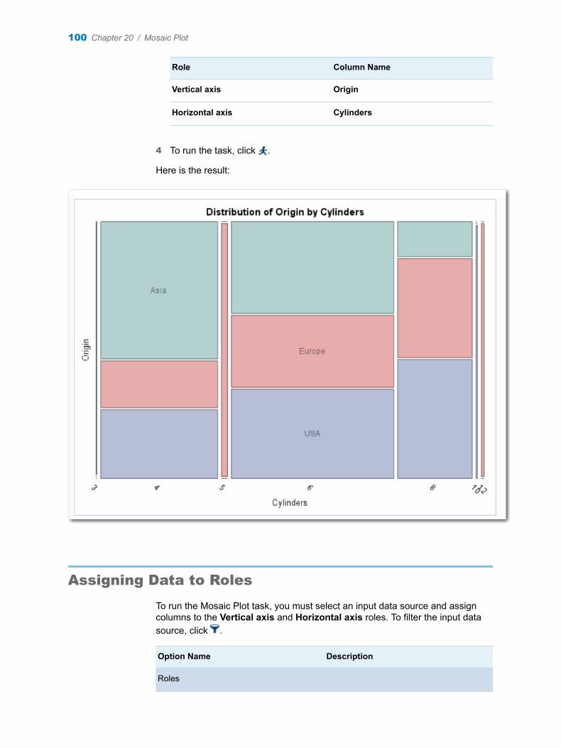
Role Column Name
Vertical axis Origin
Horizontal axis Cylinders
4 To run the task, click .
Here is the result:
Assigning Data to Roles
To run the Mosaic Plot task, you must select an input data source and assign columns to the Vertical axis and Horizontal axis roles. To filter the input data source, click .
Option Name Description
Roles
100 Chapter 20 / Mosaic Plot
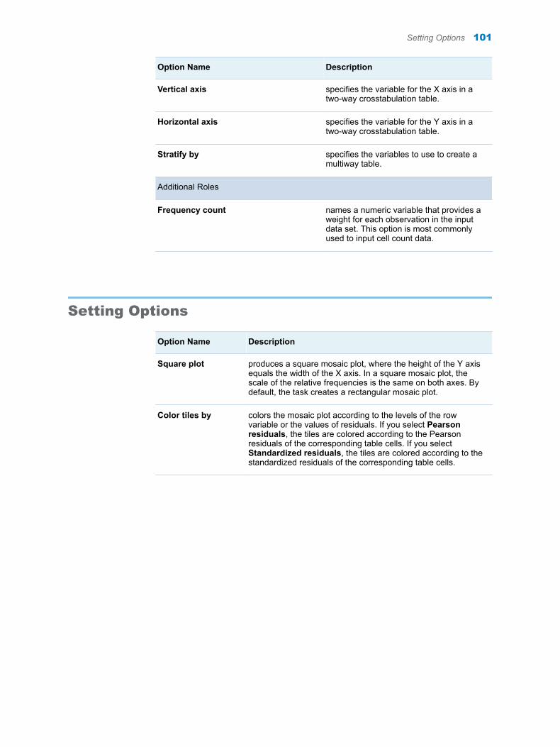
Option Name Description
Vertical axis specifies the variable for the X axis in a two-way crosstabulation table.
Horizontal axis specifies the variable for the Y axis in a two-way crosstabulation table.
Stratify by specifies the variables to use to create a multiway table.
Additional Roles
Frequency count names a numeric variable that provides a weight for each observation in the input data set. This option is most commonly used to input cell count data.
Setting Options
Option Name Description
Square plot produces a square mosaic plot, where the height of the Y axis equals the width of the X axis. In a square mosaic plot, the scale of the relative frequencies is the same on both axes. By default, the task creates a rectangular mosaic plot.
Color tiles by colors the mosaic plot according to the levels of the row variable or the values of residuals. If you select Pearson residuals, the tiles are colored according to the Pearson residuals of the corresponding table cells. If you select Standardized residuals, the tiles are colored according to the standardized residuals of the corresponding table cells.
Setting Options 101

102 Chapter 20 / Mosaic Plot
21Pie Chart
About the Pie Chart Task . . . . . . . . . . . . . . . . . . . . . . . . . . . . . . . . . . . . . . . . . . . . . . . . . . 103
Example: Pie Chart That Shows Total MSRP for Each Car Type by Region . 103
Assigning Data to Roles . . . . . . . . . . . . . . . . . . . . . . . . . . . . . . . . . . . . . . . . . . . . . . . . . . . 104
Setting Options . . . . . . . . . . . . . . . . . . . . . . . . . . . . . . . . . . . . . . . . . . . . . . . . . . . . . . . . . . . . 105
About the Pie Chart Task
The Pie Chart task creates pie charts that represent the relative contribution of the parts to the whole by displaying data as wedge-shaped "slices" of a circle. Each slice represents a category of data. The size of a slice represents the contribution of the data to the total chart statistic.
Example: Pie Chart That Shows Total MSRP for Each Car Type by Region
In this example, you want to compare the manufacturer’s suggested retail price (MSRP) for each car type grouped by region of origin. The resulting pie chart consists of six rings—one for each car type. The rings are then subset into the MSRP values for the three regions: Asia, Europe, and USA. Using this chart, you can compare the total MSRP values for each region. The ring for the SUV car type shows that the USA has the highest MSRP and that Europe has the lowest MSRP.
To create this example:
1 In the Tasks section, expand the Graph folder, and then double-click Pie Chart. The user interface for the Pie Chart task opens.
2 On the Data tab, select the SASHELP.CARS data set.
TIP If the data set is not available from the drop-down list, click . In
the Choose a Table window, expand the library that contains the data set that you want to use. Select the data set for the example and click OK. The selected data set should now appear in the drop-down list.
103
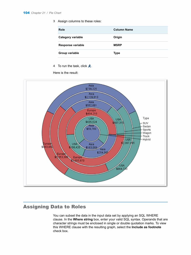
3 Assign columns to these roles:
Role Column Name
Category variable Origin
Response variable MSRP
Group variable Type
4 To run the task, click .
Here is the result:
Assigning Data to Roles
You can subset the data in the input data set by applying an SQL WHERE clause. In the Where string box, enter your valid SQL syntax. Operands that are character strings must be enclosed in single or double quotation marks. To view this WHERE clause with the resulting graph, select the Include as footnote check box.
104 Chapter 21 / Pie Chart
To run the Pie Chart task, you must assign a column to the Category variable role.
Option Name Description
Role
Category variable specifies the variable that classifies the observations into distinct subsets.
Response variable specifies a numeric response variable for the plot.
Group variable specifies a variable that is used to group the data.
URL variable specifies a character variable that contains URLs for web pages to be displayed when parts of the plot are selected within an HTML page.
Note: If the task generates an “Other” slice in the pie chart, there is not a URL associated with this slice. Therefore, this slice does not contain a link.
Orientation
Starting point specifies where to create the first slice in the pie chart. The remaining slices appear counterclockwise.
Center the first slice specifies whether to offset the first slice.
Setting Options
Option Name Description
Title and Footnote
You can specify a custom title and footnote for the output. You can also specify the font size for this text.
Pie Details
Fill transparency specifies the degree of transparency for the plot. The range is 0 (completely opaque) to 1 (completely transparent).
Data skin specifies a special effect to be used on all filled slices.
Pie Labels
Setting Options 105

Option Name Description
Location specifies whether to display the label inside or outside the slice in the pie chart. By default, the Pie Chart task determines the best location for the slice.
Set label font size enables you to specify the font size of the label for each slice.
Graph Size
You can specify the width and height of the graph in inches, centimeters, or pixels.
106 Chapter 21 / Pie Chart
22Scatter Plot
About the Scatter Plot Task . . . . . . . . . . . . . . . . . . . . . . . . . . . . . . . . . . . . . . . . . . . . . . . . 107
Example: Scatter Plot of Height versus Weight . . . . . . . . . . . . . . . . . . . . . . . . . . . . 107
Assigning Data to Roles . . . . . . . . . . . . . . . . . . . . . . . . . . . . . . . . . . . . . . . . . . . . . . . . . . . 108
Setting Options . . . . . . . . . . . . . . . . . . . . . . . . . . . . . . . . . . . . . . . . . . . . . . . . . . . . . . . . . . . . 110
About the Scatter Plot Task
The Scatter Plot task creates plots that show the relationships between two or three variables by revealing patterns or concentrations of data points. For example, a two-dimensional scatter plot can display the heights and weights of all students in a class.
Example: Scatter Plot of Height versus Weight
In this example, you want to create a scatter plot of height versus weight.
To create this example:
1 In the Tasks section, expand the Graph folder, and then double-click Scatter Plot. The user interface for the Scatter Plot task opens.
2 On the Data tab, select the SASHELP.CLASS data set.
TIP If the data set is not available from the drop-down list, click . In
the Choose a Table window, expand the library that contains the data set that you want to use. Select the data set for the example and click OK. The selected data set should now appear in the drop-down list.
3 Assign columns to these roles:
107

Role Column Name
X variable Height
Y variable Weight
4 To run the task, click .
Assigning Data to Roles
You can subset the data in the input data set by applying an SQL WHERE clause. In the Where string box, enter your valid SQL syntax. Operands that are character strings must be enclosed in single or double quotation marks. To view this WHERE clause with the resulting graph, select the Include as footnote check box.
108 Chapter 22 / Scatter Plot

To run the Scatter Plot task, you must assign columns to the X variable and Y variable role.
Option Name Description
Roles
X variable specifies the variable for the x axis.
Y variable specifies the variable for the y axis.
Group variable specifies a variable that is used to group the data. The plot elements for each group value are automatically distinguished by different visual attributes.
Marker label variable displays a label for each data point. If you specify a variable, the values of that variable are used for the data labels. If you do not specify a variable, then the values of the Y variable are used for the data labels.
URL variable specifies a character variable that contains URLs for web pages to be displayed when parts of the plot are selected within an HTML page.
Fit Plots
Note: This is available only if you assign numeric variables.
Regression creates a plot with the fitted regression line. You can specify whether to include the confidence limits for means and the prediction limits for the individual predicted values. The Alpha option specifies the confidence level for the confidence limits. The Degree option specifies the degree of the polynomial fit.
Loess creates a fitted loess curve. You can specify whether to include the confidence limits. The Alpha option specifies the confidence level for the confidence limits.
PBSpline creates a fitted penalized B-spline curve. You can specify whether to include the confidence limits for means and the prediction limits for the individual predicted values. The Alpha option specifies the confidence level for the confidence limits.
Assigning Data to Roles 109
Setting Options
Option Name Description
Title and Footnote
You can specify a custom title and footnote for the output. You can also specify the font size for this text.
Marker Details
You can specify the symbol type, color, and size of the markers. You can also specify the degree of transparency for the plot. The range is 0 (completely opaque) to 1 (completely transparent).
Marker Labels
Font size specifies the appearance of the labels in the plot when you assign a variable to the Marker label variable role.
X Axis, Y Axis
Show grid lines creates grid lines at each tick on the axis.
Show label displays the label for the axis. By default, the label is the variable name.
To customize, enter this label in the Custom label box.
Legend Details
Legend location specifies whether the legend is placed outside or inside the axis area.
Graph Size
You can specify the width and height of the graph in inches, centimeters, or pixels.
110 Chapter 22 / Scatter Plot
23Series Plot
About the Series Plot Task . . . . . . . . . . . . . . . . . . . . . . . . . . . . . . . . . . . . . . . . . . . . . . . . . 111
Example: Series Plot of Stock Trends . . . . . . . . . . . . . . . . . . . . . . . . . . . . . . . . . . . . . . 111
Assigning Data to Roles . . . . . . . . . . . . . . . . . . . . . . . . . . . . . . . . . . . . . . . . . . . . . . . . . . . 112
Setting Options . . . . . . . . . . . . . . . . . . . . . . . . . . . . . . . . . . . . . . . . . . . . . . . . . . . . . . . . . . . . 113
About the Series Plot Task
The Series Plot task creates a line plot. Series plots display a series of line segments that connect observations of input data.
Example: Series Plot of Stock Trends
In this example, you want to create a series plot that shows stock trends.
To create this example:
1 In the Tasks section, expand the Graph folder, and then double-click Series Plot. The user interface for the Series Plot task opens.
2 On the Data tab, select the SASHELP.STOCKS data set.
TIP If the data set is not available from the drop-down list, click . In
the Choose a Table window, expand the library that contains the data set that you want to use. Select the data set for the example and click OK. The selected data set should now appear in the drop-down list.
3 Assign columns to these roles:
Role Column Name
X variable Date
Y variable Open
111
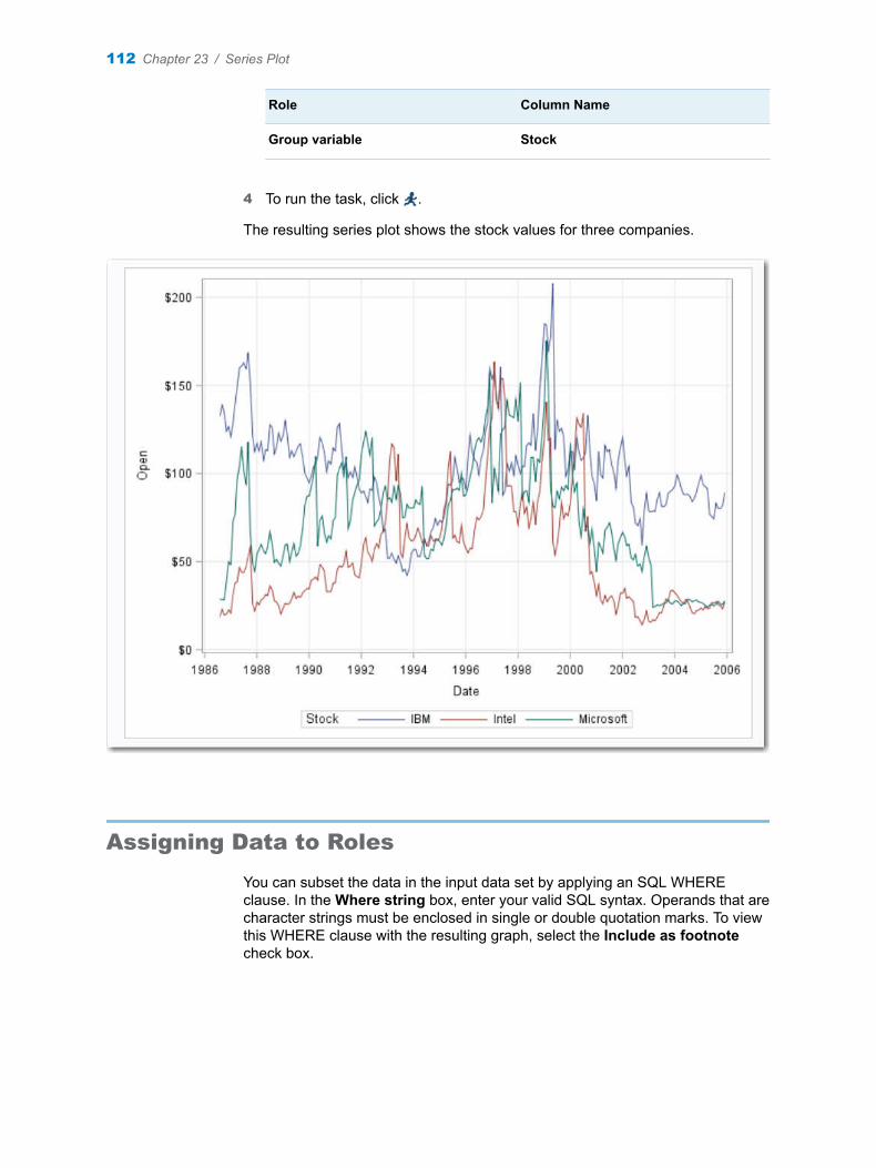
Role Column Name
Group variable Stock
4 To run the task, click .
The resulting series plot shows the stock values for three companies.
Assigning Data to Roles
You can subset the data in the input data set by applying an SQL WHERE clause. In the Where string box, enter your valid SQL syntax. Operands that are character strings must be enclosed in single or double quotation marks. To view this WHERE clause with the resulting graph, select the Include as footnote check box.
112 Chapter 23 / Series Plot
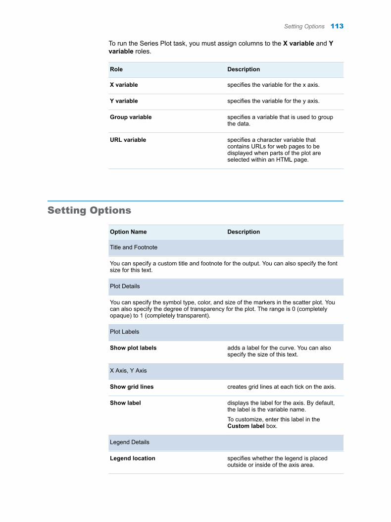
To run the Series Plot task, you must assign columns to the X variable and Y variable roles.
Role Description
X variable specifies the variable for the x axis.
Y variable specifies the variable for the y axis.
Group variable specifies a variable that is used to group the data.
URL variable specifies a character variable that contains URLs for web pages to be displayed when parts of the plot are selected within an HTML page.
Setting Options
Option Name Description
Title and Footnote
You can specify a custom title and footnote for the output. You can also specify the font size for this text.
Plot Details
You can specify the symbol type, color, and size of the markers in the scatter plot. You can also specify the degree of transparency for the plot. The range is 0 (completely opaque) to 1 (completely transparent).
Plot Labels
Show plot labels adds a label for the curve. You can also specify the size of this text.
X Axis, Y Axis
Show grid lines creates grid lines at each tick on the axis.
Show label displays the label for the axis. By default, the label is the variable name.
To customize, enter this label in the Custom label box.
Legend Details
Legend location specifies whether the legend is placed outside or inside of the axis area.
Setting Options 113

Option Name Description
Graph Size
You can specify the width and height of the graph in inches, centimeters, or pixels.
114 Chapter 23 / Series Plot
24Simple HBar
About the Simple HBar Task . . . . . . . . . . . . . . . . . . . . . . . . . . . . . . . . . . . . . . . . . . . . . . . 115
Example: Horizontal Bar Chart of Mileage by Origin and Type . . . . . . . . . . . . . . 115
Assigning Data to Roles . . . . . . . . . . . . . . . . . . . . . . . . . . . . . . . . . . . . . . . . . . . . . . . . . . . 116
Setting Options . . . . . . . . . . . . . . . . . . . . . . . . . . . . . . . . . . . . . . . . . . . . . . . . . . . . . . . . . . . . 117
About the Simple HBar Task
The Simple HBar task creates a simple horizontal bar chart. You can customize the title, footnotes, axes, and legends for the horizontal bar chart.
Example: Horizontal Bar Chart of Mileage by Origin and Type
To create this horizontal bar chart:
1 In the Tasks section, expand the Graphs folder, and then double-click Simple HBar. The user interface for the Simple HBar task opens.
2 On the Data tab, select the SASHELP.CARS data set.
TIP If the data set is not available from the drop-down list, click . In
the Choose a Table window, expand the library that contains the data set that you want to use. Select the data set for the example and click OK. The selected data set should now appear in the drop-down list.
3 Assign columns to these roles:
Role Column Name
Category variable Origin
Response variable MPG_City
115
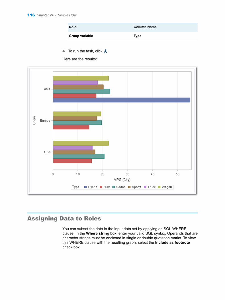
Role Column Name
Group variable Type
4 To run the task, click .
Here are the results:
Assigning Data to Roles
You can subset the data in the input data set by applying an SQL WHERE clause. In the Where string box, enter your valid SQL syntax. Operands that are character strings must be enclosed in single or double quotation marks. To view this WHERE clause with the resulting graph, select the Include as footnote check box.
116 Chapter 24 / Simple HBar
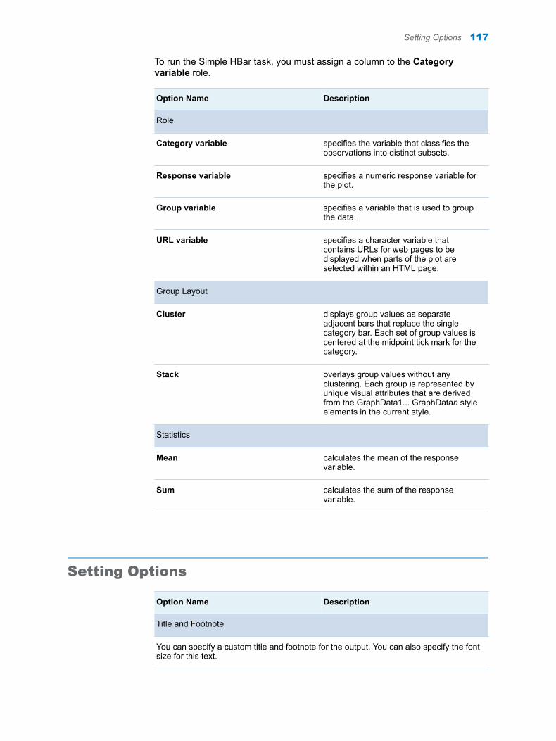
To run the Simple HBar task, you must assign a column to the Category variable role.
Option Name Description
Role
Category variable specifies the variable that classifies the observations into distinct subsets.
Response variable specifies a numeric response variable for the plot.
Group variable specifies a variable that is used to group the data.
URL variable specifies a character variable that contains URLs for web pages to be displayed when parts of the plot are selected within an HTML page.
Group Layout
Cluster displays group values as separate adjacent bars that replace the single category bar. Each set of group values is centered at the midpoint tick mark for the category.
Stack overlays group values without any clustering. Each group is represented by unique visual attributes that are derived from the GraphData1... GraphDatan style elements in the current style.
Statistics
Mean calculates the mean of the response variable.
Sum calculates the sum of the response variable.
Setting Options
Option Name Description
Title and Footnote
You can specify a custom title and footnote for the output. You can also specify the font size for this text.
Setting Options 117
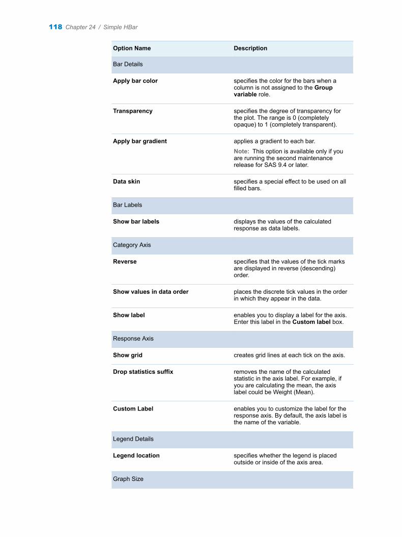
Option Name Description
Bar Details
Apply bar color specifies the color for the bars when a column is not assigned to the Group variable role.
Transparency specifies the degree of transparency for the plot. The range is 0 (completely opaque) to 1 (completely transparent).
Apply bar gradient applies a gradient to each bar.
Note: This option is available only if you are running the second maintenance release for SAS 9.4 or later.
Data skin specifies a special effect to be used on all filled bars.
Bar Labels
Show bar labels displays the values of the calculated response as data labels.
Category Axis
Reverse specifies that the values of the tick marks are displayed in reverse (descending) order.
Show values in data order places the discrete tick values in the order in which they appear in the data.
Show label enables you to display a label for the axis. Enter this label in the Custom label box.
Response Axis
Show grid creates grid lines at each tick on the axis.
Drop statistics suffix removes the name of the calculated statistic in the axis label. For example, if you are calculating the mean, the axis label could be Weight (Mean).
Custom Label enables you to customize the label for the response axis. By default, the axis label is the name of the variable.
Legend Details
Legend location specifies whether the legend is placed outside or inside of the axis area.
Graph Size
118 Chapter 24 / Simple HBar

Option Name Description
You can specify the width and height of the graph in inches, centimeters, or pixels.
Setting Options 119

120 Chapter 24 / Simple HBar

Part 3
Combinatorics and Probability Tasks
Chapter 25Permutations . . . . . . . . . . . . . . . . . . . . . . . . . . . . . . . . . . . . . . . . . . . . . . . . . . . 123
Chapter 26Combinations . . . . . . . . . . . . . . . . . . . . . . . . . . . . . . . . . . . . . . . . . . . . . . . . . . . 125
Chapter 27Same Birthday Probability . . . . . . . . . . . . . . . . . . . . . . . . . . . . . . . . . . . . . . . . 127
Chapter 28Dice Roll Simulation . . . . . . . . . . . . . . . . . . . . . . . . . . . . . . . . . . . . . . . . . . . . . 129
Chapter 29Coin Toss Simulation . . . . . . . . . . . . . . . . . . . . . . . . . . . . . . . . . . . . . . . . . . . . 131
Chapter 30Poker Hand Probability . . . . . . . . . . . . . . . . . . . . . . . . . . . . . . . . . . . . . . . . . . . 133
121

122
25Permutations
About the Permutations Task . . . . . . . . . . . . . . . . . . . . . . . . . . . . . . . . . . . . . . . . . . . . . . 123
Example: Calculating the Permutations of Six Objects . . . . . . . . . . . . . . . . . . . . . 123
Setting Options . . . . . . . . . . . . . . . . . . . . . . . . . . . . . . . . . . . . . . . . . . . . . . . . . . . . . . . . . . . . 124
About the Permutations Task
The Permutations task computes the possible permutations of a given number of objects.
Example: Calculating the Permutations of Six Objects
To create this example:
1 In the Tasks section, expand the Combinatorics and Probability folder, and then double-click Permutations. The user interface for the Permutations task opens.
2 On the Options tab, specify these options.
Assign columns to these roles:
Option Name Value to Specify
Number of objects 6
Data set name Perms
3 To run the task, click .
123
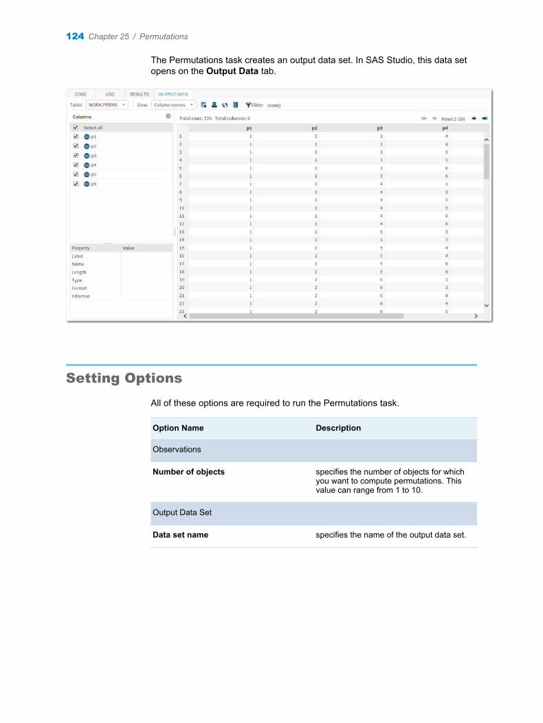
The Permutations task creates an output data set. In SAS Studio, this data set opens on the Output Data tab.
Setting Options
All of these options are required to run the Permutations task.
Option Name Description
Observations
Number of objects specifies the number of objects for which you want to compute permutations. This value can range from 1 to 10.
Output Data Set
Data set name specifies the name of the output data set.
124 Chapter 25 / Permutations
26Combinations
About the Combinations Task . . . . . . . . . . . . . . . . . . . . . . . . . . . . . . . . . . . . . . . . . . . . . 125
Example: Calculating the Combinations of 52 Objects in 5 Sets . . . . . . . . . . . . 125
Setting Options . . . . . . . . . . . . . . . . . . . . . . . . . . . . . . . . . . . . . . . . . . . . . . . . . . . . . . . . . . . . 126
About the Combinations Task
The Combinations task computes the possible combinations of the total number of objects into sets with a specified number in each set.
Example: Calculating the Combinations of 52 Objects in 5 Sets
To create this example:
1 In the Tasks section, expand the Combinatorics and Probability folder, and then double-click Combinations. The user interface for the Combinations task opens.
2 On the Options tab, specify these options.
Assign columns to these roles:
Option Name Value to Specify
Total number of objects 52
Number of objects in a set 5
Data set name Combo
3 To run the task, click .
125
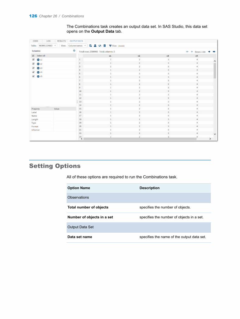
The Combinations task creates an output data set. In SAS Studio, this data set opens on the Output Data tab.
Setting Options
All of these options are required to run the Combinations task.
Option Name Description
Observations
Total number of objects specifies the number of objects.
Number of objects in a set specifies the number of objects in a set.
Output Data Set
Data set name specifies the name of the output data set.
126 Chapter 26 / Combinations
27Same Birthday Probability
About the Same Birthday Probability Task . . . . . . . . . . . . . . . . . . . . . . . . . . . . . . . . . 127
Example: Probability of Two or More People Sharing a Birthday in a Room of 145 People . . . . . . . . . . . . . . . . . . . . . . . . . . . . . . . . . . . . . . . . . 127
Setting Options . . . . . . . . . . . . . . . . . . . . . . . . . . . . . . . . . . . . . . . . . . . . . . . . . . . . . . . . . . . . 128
About the Same Birthday Probability Task
The Same Birthday Probability task computes the probability that two or more people in a room have the same birthday.
Example: Probability of Two or More People Sharing a Birthday in a Room of 145 People
To create this example:
1 In the Tasks section, expand the Combinatorics and Probability folder, and then double-click Same Birthday Probability. The user interface for the Same Birthday Probability task opens.
2 On the Options tab, specify these options.
Option Name Value to Specify
Number in a room 145
Data set name Birthdays
3 To run the task, click .
127
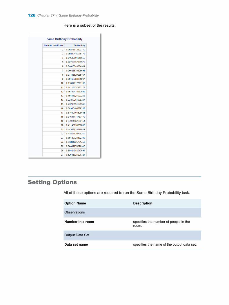
Here is a subset of the results:
Setting Options
All of these options are required to run the Same Birthday Probability task.
Option Name Description
Observations
Number in a room specifies the number of people in the room.
Output Data Set
Data set name specifies the name of the output data set.
128 Chapter 27 / Same Birthday Probability

28Dice Roll Simulation
About the Dice Roll Simulation Task . . . . . . . . . . . . . . . . . . . . . . . . . . . . . . . . . . . . . . . 129
Example: Probability of Outcomes for 100,000,000 Dice Rolls . . . . . . . . . . . . . . 129
Setting Options . . . . . . . . . . . . . . . . . . . . . . . . . . . . . . . . . . . . . . . . . . . . . . . . . . . . . . . . . . . . 130
About the Dice Roll Simulation Task
The Dice Roll Simulation task simulates rolling a specified number of dice. The results show the frequency and percentage of each possible roll given a specified number of throws.
Example: Probability of Outcomes for 100,000,000 Dice Rolls
To create this example:
1 In the Tasks section, expand the Combinatorics and Probability folder, and then double-click Dice Roll Simulation. The user interface for the Dice Roll Simulation task opens.
2 On the Options tab, specify these options.
Option Name Value to Specify
Number of dice 2
Number of rolls 100,000,000
Data set name Dice
3 To run the task, click .
129
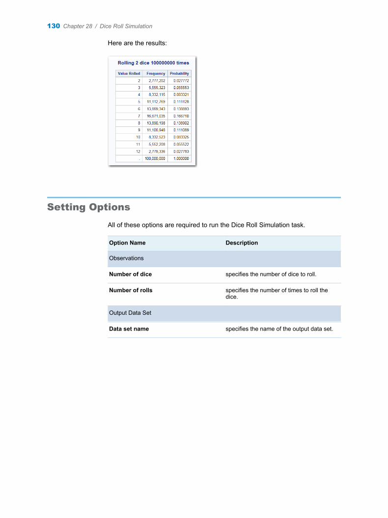
Here are the results:
Setting Options
All of these options are required to run the Dice Roll Simulation task.
Option Name Description
Observations
Number of dice specifies the number of dice to roll.
Number of rolls specifies the number of times to roll the dice.
Output Data Set
Data set name specifies the name of the output data set.
130 Chapter 28 / Dice Roll Simulation
29Coin Toss Simulation
About the Coin Toss Simulation Task . . . . . . . . . . . . . . . . . . . . . . . . . . . . . . . . . . . . . . 131
Example: Probability of Outcomes for 10,000,000 Coin Tosses . . . . . . . . . . . . . 131
Setting Options . . . . . . . . . . . . . . . . . . . . . . . . . . . . . . . . . . . . . . . . . . . . . . . . . . . . . . . . . . . . 132
About the Coin Toss Simulation Task
The Coin Toss Simulation task simulates the tossing of a specified number of coins. The results show the frequency and percentage of occurrences that the coin displays heads given a specified number of tosses.
Example: Probability of Outcomes for 10,000,000 Coin Tosses
To create this example:
1 In the Tasks section, expand the Combinatorics and Probability folder, and then double-click Coin Toss Simulation. The user interface for the Coin Toss Simulations task opens.
2 On the Options tab, specify these options.
Option Name Value to Specify
Number of coins 10
Number of tosses 10,000,000
Data set name Coins
3 To run the task, click .
131
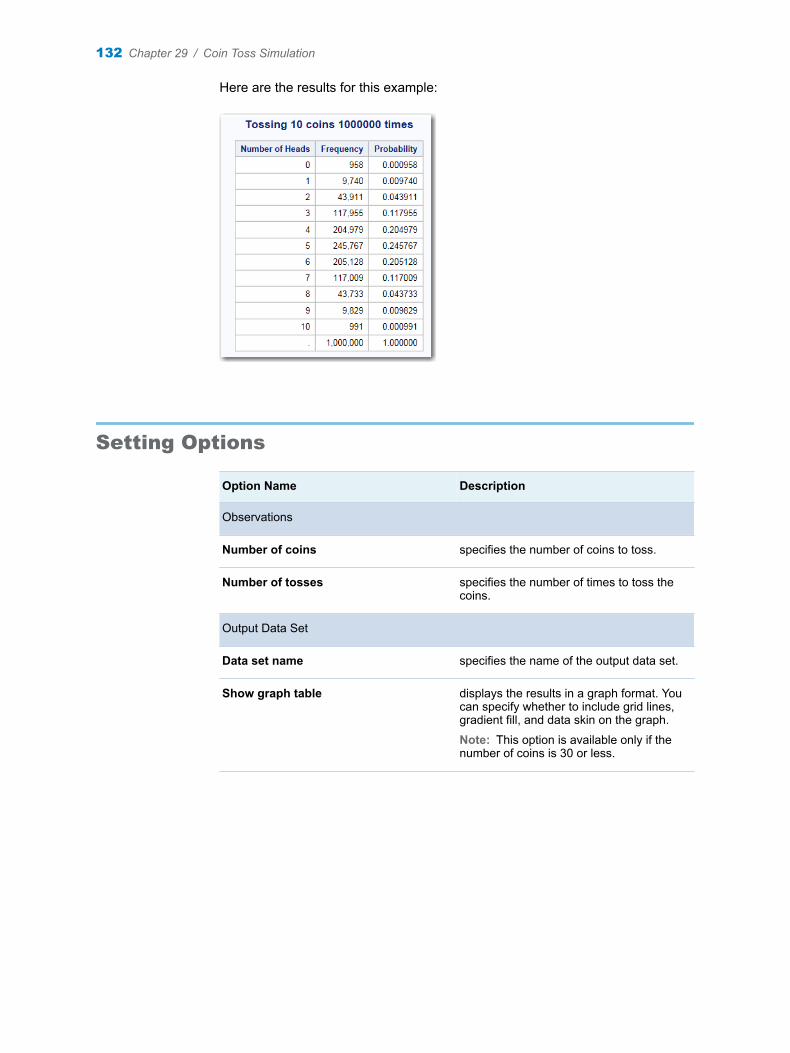
Here are the results for this example:
Setting Options
Option Name Description
Observations
Number of coins specifies the number of coins to toss.
Number of tosses specifies the number of times to toss the coins.
Output Data Set
Data set name specifies the name of the output data set.
Show graph table displays the results in a graph format. You can specify whether to include grid lines, gradient fill, and data skin on the graph.
Note: This option is available only if the number of coins is 30 or less.
132 Chapter 29 / Coin Toss Simulation

30Poker Hand Probability
About the Poker Hand Probability Task . . . . . . . . . . . . . . . . . . . . . . . . . . . . . . . . . . . . 133
Example: Results from the Poker Hand Probability Task . . . . . . . . . . . . . . . . . . . 133
About the Poker Hand Probability Task
The Poker Hand Probability task calculates the frequency and probability of poker hands. The input data set for the Poker Hand Probability task must be the output data set generated by the Computations task.
Example: Results from the Poker Hand Probability Task
To create this example:
1 In the Tasks section, expand the Combinatorics and Probability folder and double-click Poker Hand Probability. The user interface for the Poker Hand Probability task opens.
2 On the Options tab, select the WORK.COMBO data set.
Note: You must run the Combinations task to generate this data set.
3 To run the task, click . The Work.Combo data set is created.
4 In the Tasks section, expand the Combinatorics and Probability folder, and then double-click Poker Hand Probability. The user interface for the Poker Hand Probability task opens.
5 For the input data set, select WORK.COMBO.
6 To run the task, click .
133
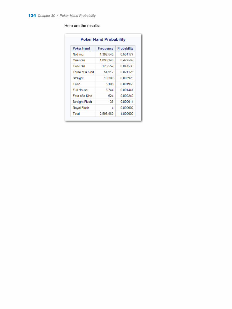
Here are the results:
134 Chapter 30 / Poker Hand Probability
Part 4
Statistics Tasks
Chapter 31Data Exploration . . . . . . . . . . . . . . . . . . . . . . . . . . . . . . . . . . . . . . . . . . . . . . . . 137
Chapter 32Summary Statistics . . . . . . . . . . . . . . . . . . . . . . . . . . . . . . . . . . . . . . . . . . . . . . 143
Chapter 33Distribution Analysis . . . . . . . . . . . . . . . . . . . . . . . . . . . . . . . . . . . . . . . . . . . . 151
Chapter 34One-Way Frequencies . . . . . . . . . . . . . . . . . . . . . . . . . . . . . . . . . . . . . . . . . . . . 157
Chapter 35Correlation Analysis . . . . . . . . . . . . . . . . . . . . . . . . . . . . . . . . . . . . . . . . . . . . . 163
Chapter 36Table Analysis . . . . . . . . . . . . . . . . . . . . . . . . . . . . . . . . . . . . . . . . . . . . . . . . . . 169
Chapter 37t Tests . . . . . . . . . . . . . . . . . . . . . . . . . . . . . . . . . . . . . . . . . . . . . . . . . . . . . . . . . 175
Chapter 38One-Way ANOVA . . . . . . . . . . . . . . . . . . . . . . . . . . . . . . . . . . . . . . . . . . . . . . . . 191
Chapter 39Nonparametric One-Way ANOVA . . . . . . . . . . . . . . . . . . . . . . . . . . . . . . . . . . 199
135
Chapter 40N-Way ANOVA . . . . . . . . . . . . . . . . . . . . . . . . . . . . . . . . . . . . . . . . . . . . . . . . . . 205
Chapter 41Analysis of Covariance . . . . . . . . . . . . . . . . . . . . . . . . . . . . . . . . . . . . . . . . . . . 211
Chapter 42Linear Regression . . . . . . . . . . . . . . . . . . . . . . . . . . . . . . . . . . . . . . . . . . . . . . . 217
Chapter 43Binary Logistic Regression . . . . . . . . . . . . . . . . . . . . . . . . . . . . . . . . . . . . . . . 231
Chapter 44Predictive Regression Models . . . . . . . . . . . . . . . . . . . . . . . . . . . . . . . . . . . . 245
Chapter 45Generalized Linear Models . . . . . . . . . . . . . . . . . . . . . . . . . . . . . . . . . . . . . . . 259
Chapter 46Mixed Models . . . . . . . . . . . . . . . . . . . . . . . . . . . . . . . . . . . . . . . . . . . . . . . . . . . 271
Chapter 47Partial Least Squares Regression . . . . . . . . . . . . . . . . . . . . . . . . . . . . . . . . . 283
136

31Data Exploration
About the Data Exploration Task . . . . . . . . . . . . . . . . . . . . . . . . . . . . . . . . . . . . . . . . . . . 137
Example: Exploring the SASHELP.CARS Data . . . . . . . . . . . . . . . . . . . . . . . . . . . . . 137
Assigning Data to Roles . . . . . . . . . . . . . . . . . . . . . . . . . . . . . . . . . . . . . . . . . . . . . . . . . . . 139
Setting the Plot Options . . . . . . . . . . . . . . . . . . . . . . . . . . . . . . . . . . . . . . . . . . . . . . . . . . . 139
About the Data Exploration Task
The Data Exploration task provides graphs that can be used to explore the relationships among selected variables.
Note: You must have SAS/STAT to use this task.
Example: Exploring the SASHELP.CARS Data
To create this example:
1 In the Tasks section, expand the Statistics folder, and then double-click Data Exploration. The user interface for the Data Exploration task opens.
2 On the Data tab, select the SASHELP.CARS data set.
TIP If the data set is not available from the drop-down list, click . In
the Choose a Table window, expand the library that contains the data set that you want to use. Select the data set for the example and click OK. The selected data set should now appear in the drop-down list.
3 Assign columns to these roles:
137
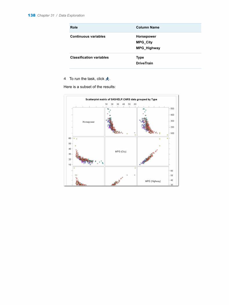
Role Column Name
Continuous variables HorsepowerMPG_CityMPG_Highway
Classification variables TypeDriveTrain
4 To run the task, click .
Here is a subset of the results:
138 Chapter 31 / Data Exploration
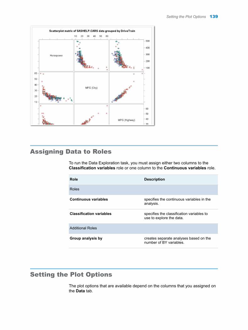
Assigning Data to Roles
To run the Data Exploration task, you must assign either two columns to the Classification variables role or one column to the Continuous variables role.
Role Description
Roles
Continuous variables specifies the continuous variables in the analysis.
Classification variables specifies the classification variables to use to explore the data.
Additional Roles
Group analysis by creates separate analyses based on the number of BY variables.
Setting the Plot Options
The plot options that are available depend on the columns that you assigned on the Data tab.
Setting the Plot Options 139
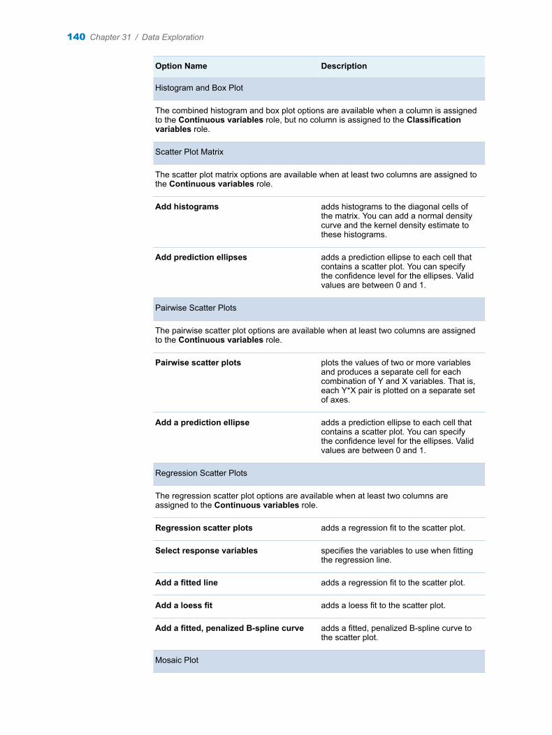
Option Name Description
Histogram and Box Plot
The combined histogram and box plot options are available when a column is assigned to the Continuous variables role, but no column is assigned to the Classification variables role.
Scatter Plot Matrix
The scatter plot matrix options are available when at least two columns are assigned to the Continuous variables role.
Add histograms adds histograms to the diagonal cells of the matrix. You can add a normal density curve and the kernel density estimate to these histograms.
Add prediction ellipses adds a prediction ellipse to each cell that contains a scatter plot. You can specify the confidence level for the ellipses. Valid values are between 0 and 1.
Pairwise Scatter Plots
The pairwise scatter plot options are available when at least two columns are assigned to the Continuous variables role.
Pairwise scatter plots plots the values of two or more variables and produces a separate cell for each combination of Y and X variables. That is, each Y*X pair is plotted on a separate set of axes.
Add a prediction ellipse adds a prediction ellipse to each cell that contains a scatter plot. You can specify the confidence level for the ellipses. Valid values are between 0 and 1.
Regression Scatter Plots
The regression scatter plot options are available when at least two columns are assigned to the Continuous variables role.
Regression scatter plots adds a regression fit to the scatter plot.
Select response variables specifies the variables to use when fitting the regression line.
Add a fitted line adds a regression fit to the scatter plot.
Add a loess fit adds a loess fit to the scatter plot.
Add a fitted, penalized B-spline curve adds a fitted, penalized B-spline curve to the scatter plot.
Mosaic Plot
140 Chapter 31 / Data Exploration
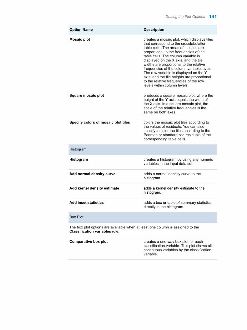
Option Name Description
Mosaic plot creates a mosaic plot, which displays tiles that correspond to the crosstabulation table cells. The areas of the tiles are proportional to the frequencies of the table cells. The column variable is displayed on the X axis, and the tile widths are proportional to the relative frequencies of the column variable levels. The row variable is displayed on the Y axis, and the tile heights are proportional to the relative frequencies of the row levels within column levels.
Square mosaic plot produces a square mosaic plot, where the height of the Y axis equals the width of the X axis. In a square mosaic plot, the scale of the relative frequencies is the same on both axes.
Specify colors of mosaic plot tiles colors the mosaic plot tiles according to the values of residuals. You can also specify to color the tiles according to the Pearson or standardized residuals of the corresponding table cells.
Histogram
Histogram creates a histogram by using any numeric variables in the input data set.
Add normal density curve adds a normal density curve to the histogram.
Add kernel density estimate adds a kernel density estimate to the histogram.
Add inset statistics adds a box or table of summary statistics directly in the histogram.
Box Plot
The box plot options are available when at least one column is assigned to the Classification variables role.
Comparative box plot creates a one-way box plot for each classification variable. This plot shows all continuous variables by the classification variable.
Setting the Plot Options 141

142 Chapter 31 / Data Exploration
32Summary Statistics
About the Summary Statistics Task . . . . . . . . . . . . . . . . . . . . . . . . . . . . . . . . . . . . . . . . 143
Example: Summary Statistics of Unit Sales . . . . . . . . . . . . . . . . . . . . . . . . . . . . . . . . 143
Assigning Data to Roles . . . . . . . . . . . . . . . . . . . . . . . . . . . . . . . . . . . . . . . . . . . . . . . . . . . 144
Setting Options . . . . . . . . . . . . . . . . . . . . . . . . . . . . . . . . . . . . . . . . . . . . . . . . . . . . . . . . . . . . 145
Setting the Output Options . . . . . . . . . . . . . . . . . . . . . . . . . . . . . . . . . . . . . . . . . . . . . . . . 149
About the Summary Statistics Task
The Summary Statistics task provides descriptive statistics for variables across all observations and within groups of observations. You can also summarize your data in a graphical display, such as histograms and box plots.
For example, you could use this task to create a report on the number of new sales, arranged by product type and country.
Note: You must license and install SAS/STAT to use this task.
Example: Summary Statistics of Unit Sales
In this example, you want to analyze unit sales. In addition to the tabular results, you choose to display a histogram of the distribution.
To create this example:
1 In the Tasks section, expand the Statistics folder, and then double-click Summary Statistics. The user interface for the Summary Statistics task opens.
2 On the Data tab, select the SASHELP.PRICEDATA data set.
TIP If the data set is not available from the drop-down list, click . In
the Choose a Table window, expand the library that contains the data set that you want to use. Select the data set for the example and click OK. The selected data set should now appear in the drop-down list.
143
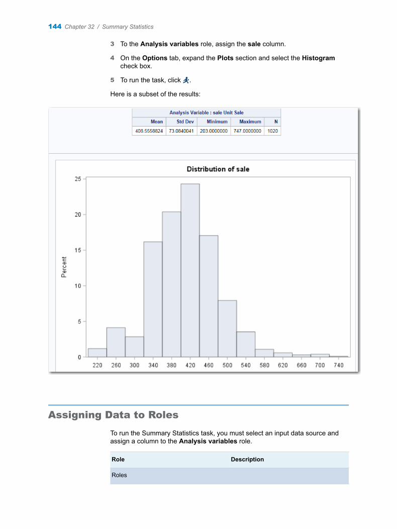
3 To the Analysis variables role, assign the sale column.
4 On the Options tab, expand the Plots section and select the Histogram check box.
5 To run the task, click .
Here is a subset of the results:
Assigning Data to Roles
To run the Summary Statistics task, you must select an input data source and assign a column to the Analysis variables role.
Role Description
Roles
144 Chapter 32 / Summary Statistics

Role Description
Analysis variables specifies the numeric variables for which you want statistics. You must assign at least one variable to this role.
Classification variables specifies the character or discrete numeric variables that are used to divide the input data into categories or subgroups. The statistics are calculated on all selected analysis variables for each unique combination of classification variables.
Additional Roles
Group analysis by enables you to obtain separate analyses of observations for each unique group.
Frequency count lists a numeric variable whose value represents the frequency of the observation. If you assign a variable to this role, the task assumes that each observation represents n observations, where n is the value of the frequency variable. If n is not an integer, SAS truncates it. If n is less than 1 or is missing, the observation is excluded from the analysis. The sum of the frequency variable represents the total number of observations.
Weight variable If you assign a variable to this role, the value of the variable for each observation is used to calculate weighted means, variances, and sums. You can assign a maximum of one variable to this role.
Setting Options
Option Name Description
Statistics
Basic Statistics
Mean is the arithmetic average, calculated by adding the values of an analysis variable and dividing this sum by the number of nonmissing observations.
Setting Options 145
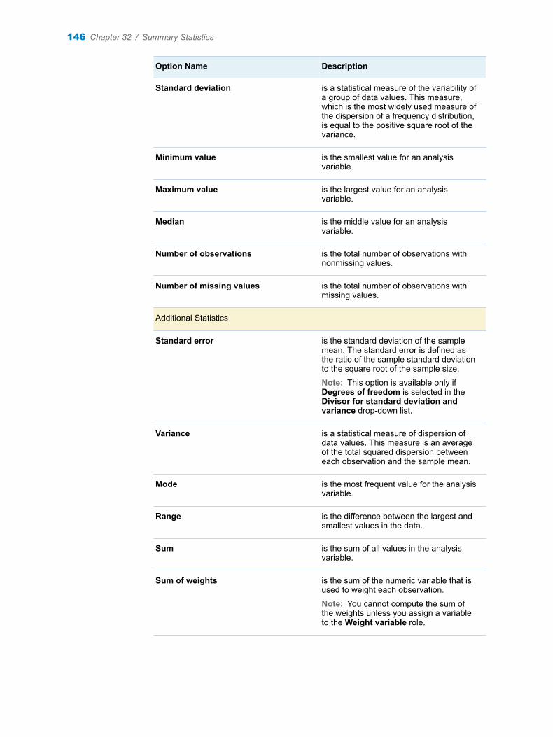
Option Name Description
Standard deviation is a statistical measure of the variability of a group of data values. This measure, which is the most widely used measure of the dispersion of a frequency distribution, is equal to the positive square root of the variance.
Minimum value is the smallest value for an analysis variable.
Maximum value is the largest value for an analysis variable.
Median is the middle value for an analysis variable.
Number of observations is the total number of observations with nonmissing values.
Number of missing values is the total number of observations with missing values.
Additional Statistics
Standard error is the standard deviation of the sample mean. The standard error is defined as the ratio of the sample standard deviation to the square root of the sample size.
Note: This option is available only if Degrees of freedom is selected in the Divisor for standard deviation and variance drop-down list.
Variance is a statistical measure of dispersion of data values. This measure is an average of the total squared dispersion between each observation and the sample mean.
Mode is the most frequent value for the analysis variable.
Range is the difference between the largest and smallest values in the data.
Sum is the sum of all values in the analysis variable.
Sum of weights is the sum of the numeric variable that is used to weight each observation.
Note: You cannot compute the sum of the weights unless you assign a variable to the Weight variable role.
146 Chapter 32 / Summary Statistics
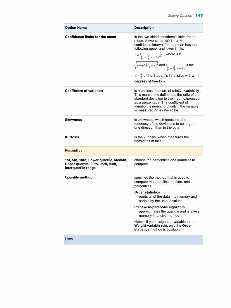
Option Name Description
Confidence limits for the mean is the two-sided confidence limits for the mean. A two-sided 100 1 − α %confidence interval for the mean has the following upper and lower limits:x ± t
1 − α2 ; n − 1
sn , where s is
1n − 1Σ xi − x 2 and t
1 − α2 ; n − 1
is the
1 − α2 of the Student’s t statistics with n − 1
degrees of freedom.
Coefficient of variation is a unitless measure of relative variability. This measure is defined as the ratio of the standard deviation to the mean expressed as a percentage. The coefficient of variation is meaningful only if the variable is measured on a ratio scale.
Skewness is skewness, which measures the tendency of the deviations to be larger in one direction than in the other.
Kurtosis is the kurtosis, which measures the heaviness of tails.
Percentiles
1st, 5th, 10th, Lower quartile, Median, Upper quartile, 90th, 95th, 99th, Interquartile range
choose the percentiles and quantiles to compute.
Quantile method specifies the method that is used to compute the quantiles, median, and percentiles.
Order statisticsreads all of the data into memory and sorts it by the unique values.
Piecewise-parabolic algorithmapproximates the quantile and is a less memory-intensive method.
Note: If you assigned a variable to the Weight variable role, only the Order statistics method is available.
Plots
Setting Options 147
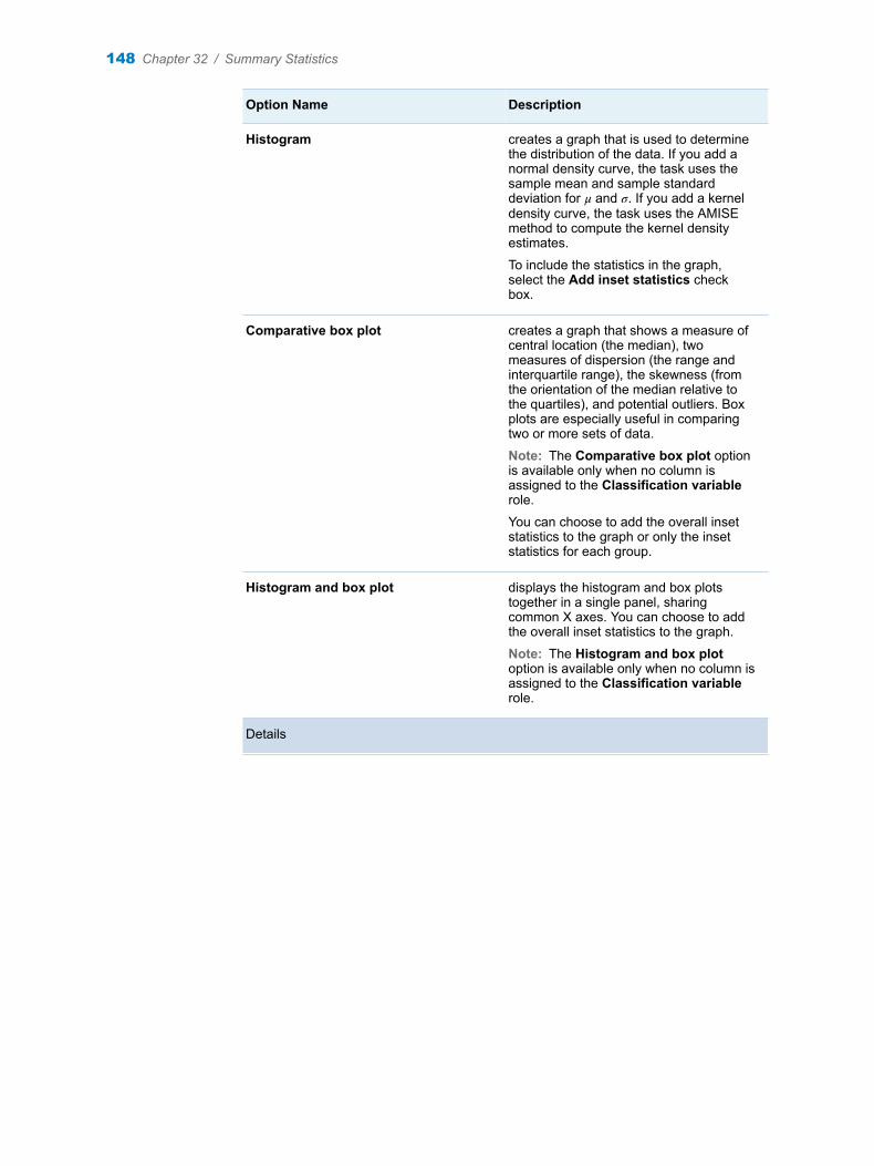
Option Name Description
Histogram creates a graph that is used to determine the distribution of the data. If you add a normal density curve, the task uses the sample mean and sample standard deviation for μ and σ. If you add a kernel density curve, the task uses the AMISE method to compute the kernel density estimates.
To include the statistics in the graph, select the Add inset statistics check box.
Comparative box plot creates a graph that shows a measure of central location (the median), two measures of dispersion (the range and interquartile range), the skewness (from the orientation of the median relative to the quartiles), and potential outliers. Box plots are especially useful in comparing two or more sets of data.
Note: The Comparative box plot option is available only when no column is assigned to the Classification variable role.
You can choose to add the overall inset statistics to the graph or only the inset statistics for each group.
Histogram and box plot displays the histogram and box plots together in a single panel, sharing common X axes. You can choose to add the overall inset statistics to the graph.
Note: The Histogram and box plot option is available only when no column is assigned to the Classification variable role.
Details
148 Chapter 32 / Summary Statistics
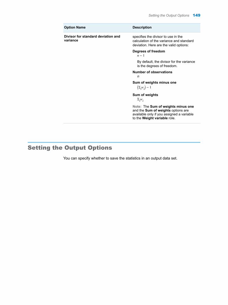
Option Name Description
Divisor for standard deviation and variance
specifies the divisor to use in the calculation of the variance and standard deviation. Here are the valid options:
Degrees of freedomn − 1By default, the divisor for the variance is the degrees of freedom.
Number of observationsn
Sum of weights minus oneΣiwi − 1
Sum of weightsΣiwi
Note: The Sum of weights minus one and the Sum of weights options are available only if you assigned a variable to the Weight variable role.
Setting the Output Options
You can specify whether to save the statistics in an output data set.
Setting the Output Options 149

150 Chapter 32 / Summary Statistics
33Distribution Analysis
About the Distribution Analysis Task . . . . . . . . . . . . . . . . . . . . . . . . . . . . . . . . . . . . . . 151
Example: Distribution Analysis of Sales for Each Region . . . . . . . . . . . . . . . . . . 151
Assigning Data to Roles . . . . . . . . . . . . . . . . . . . . . . . . . . . . . . . . . . . . . . . . . . . . . . . . . . . 153
Setting Options . . . . . . . . . . . . . . . . . . . . . . . . . . . . . . . . . . . . . . . . . . . . . . . . . . . . . . . . . . . . 154
About the Distribution Analysis Task
Distribution analysis provides information about the distribution of numeric variables. A variety of plots such as histograms, probability plots, and quantile-quantile plots can be used in this analysis.
Note: You must have SAS/STAT licensed and installed to use this task.
Example: Distribution Analysis of Sales for Each Region
In this example, you want to analyze the sales for each region. Because the data contains three regions, you get three sets of results.
To create this example:
1 In the Tasks section, expand the Statistics folder, and then double-click Distribution Analysis. The user interface for the Distribution Analysis task opens.
2 On the Data tab, select the SASHELP.PRICEDATA data set.
TIP If the data set is not available from the drop-down list, click . In
the Choose a Table window, expand the library that contains the data set that you want to use. Select the data set for the example and click OK. The selected data set should now appear in the drop-down list.
3 To the Analysis variables role, assign the sale variable.
151
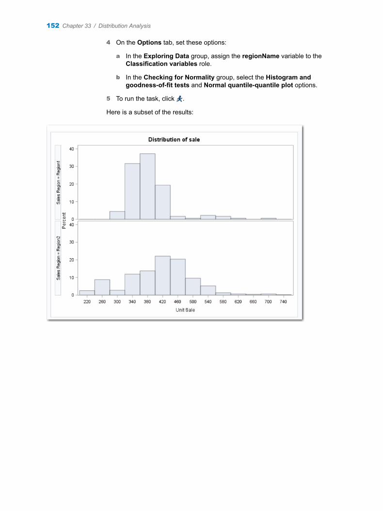
4 On the Options tab, set these options:
a In the Exploring Data group, assign the regionName variable to the Classification variables role.
b In the Checking for Normality group, select the Histogram and goodness-of-fit tests and Normal quantile-quantile plot options.
5 To run the task, click .
Here is a subset of the results:
152 Chapter 33 / Distribution Analysis
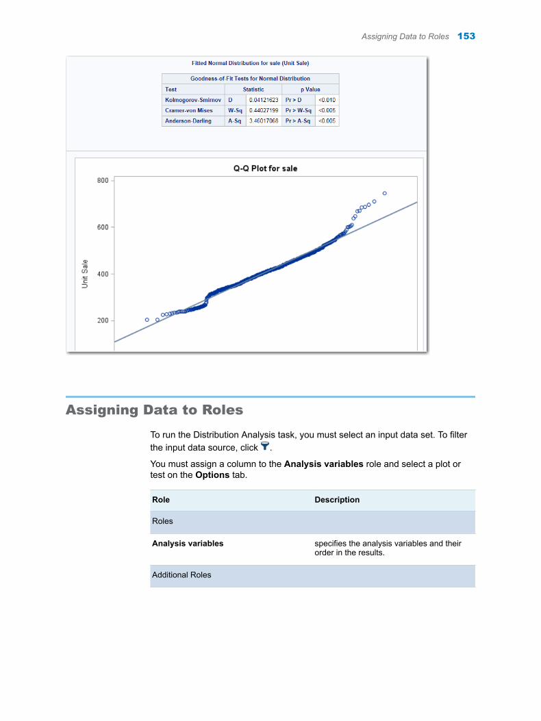
Assigning Data to Roles
To run the Distribution Analysis task, you must select an input data set. To filter the input data source, click .
You must assign a column to the Analysis variables role and select a plot or test on the Options tab.
Role Description
Roles
Analysis variables specifies the analysis variables and their order in the results.
Additional Roles
Assigning Data to Roles 153
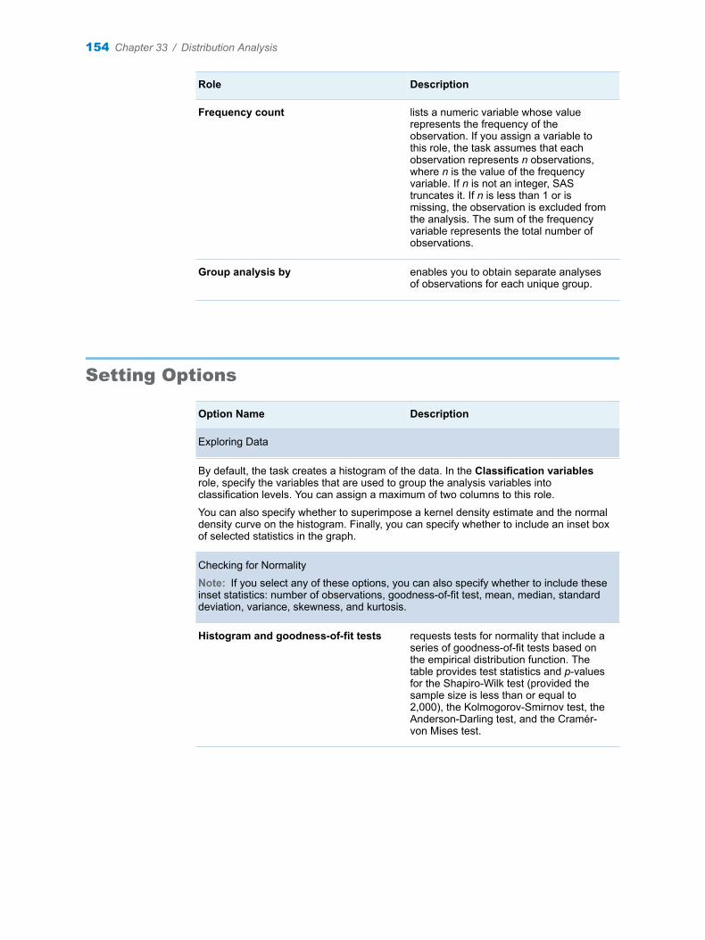
Role Description
Frequency count lists a numeric variable whose value represents the frequency of the observation. If you assign a variable to this role, the task assumes that each observation represents n observations, where n is the value of the frequency variable. If n is not an integer, SAS truncates it. If n is less than 1 or is missing, the observation is excluded from the analysis. The sum of the frequency variable represents the total number of observations.
Group analysis by enables you to obtain separate analyses of observations for each unique group.
Setting Options
Option Name Description
Exploring Data
By default, the task creates a histogram of the data. In the Classification variables role, specify the variables that are used to group the analysis variables into classification levels. You can assign a maximum of two columns to this role.
You can also specify whether to superimpose a kernel density estimate and the normal density curve on the histogram. Finally, you can specify whether to include an inset box of selected statistics in the graph.
Checking for Normality
Note: If you select any of these options, you can also specify whether to include these inset statistics: number of observations, goodness-of-fit test, mean, median, standard deviation, variance, skewness, and kurtosis.
Histogram and goodness-of-fit tests requests tests for normality that include a series of goodness-of-fit tests based on the empirical distribution function. The table provides test statistics and p-values for the Shapiro-Wilk test (provided the sample size is less than or equal to 2,000), the Kolmogorov-Smirnov test, the Anderson-Darling test, and the Cramér-von Mises test.
154 Chapter 33 / Distribution Analysis
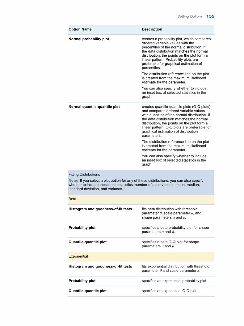
Option Name Description
Normal probability plot creates a probability plot, which compares ordered variable values with the percentiles of the normal distribution. If the data distribution matches the normal distribution, the points on the plot form a linear pattern. Probability plots are preferable for graphical estimation of percentiles.
The distribution reference line on the plot is created from the maximum likelihood estimate for the parameter.
You can also specify whether to include an inset box of selected statistics in the graph.
Normal quantile-quantile plot creates quantile-quantile plots (Q-Q plots) and compares ordered variable values with quantiles of the normal distribution. If the data distribution matches the normal distribution, the points on the plot form a linear pattern. Q-Q plots are preferable for graphical estimation of distribution parameters.
The distribution reference line on the plot is created from the maximum likelihood estimate for the parameter.
You can also specify whether to include an inset box of selected statistics in the graph.
Fitting Distributions
Note: If you select a plot option for any of these distributions, you can also specify whether to include these inset statistics: number of observations, mean, median, standard deviation, and variance.
Beta
Histogram and goodness-of-fit tests fits beta distribution with threshold parameter θ, scale parameter σ, and shape parameters α and β.
Probability plot specifies a beta probability plot for shape parameters α and β.
Quantile-quantile plot specifies a beta Q-Q plot for shape parameters α and β.
Exponential
Histogram and goodness-of-fit tests fits exponential distribution with threshold parameter θ and scale parameter σ.
Probability plot specifies an exponential probability plot.
Quantile-quantile plot specifies an exponential Q-Q plot.
Setting Options 155
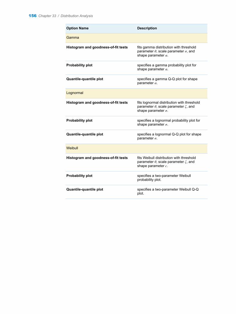
Option Name Description
Gamma
Histogram and goodness-of-fit tests fits gamma distribution with threshold parameter θ, scale parameter σ, and shape parameter α.
Probability plot specifies a gamma probability plot for shape parameter α.
Quantile-quantile plot specifies a gamma Q-Q plot for shape parameter α.
Lognormal
Histogram and goodness-of-fit tests fits lognormal distribution with threshold parameter θ, scale parameter ζ, and shape parameter σ.
Probability plot specifies a lognormal probability plot for shape parameter σ.
Quantile-quantile plot specifies a lognormal Q-Q plot for shape parameter σ.
Weibull
Histogram and goodness-of-fit tests fits Weibull distribution with threshold parameter θ, scale parameter ζ, and shape parameter c.
Probability plot specifies a two-parameter Weibull probability plot.
Quantile-quantile plot specifies a two-parameter Weibull Q-Q plot.
156 Chapter 33 / Distribution Analysis

34One-Way Frequencies
About the One-Way Frequencies Task . . . . . . . . . . . . . . . . . . . . . . . . . . . . . . . . . . . . . 157
Example: One-Way Frequencies of Unit Sales . . . . . . . . . . . . . . . . . . . . . . . . . . . . . 157
Assigning Data to Roles . . . . . . . . . . . . . . . . . . . . . . . . . . . . . . . . . . . . . . . . . . . . . . . . . . . 159
Setting Options . . . . . . . . . . . . . . . . . . . . . . . . . . . . . . . . . . . . . . . . . . . . . . . . . . . . . . . . . . . . 160
About the One-Way Frequencies Task
The One-Way Frequencies task generates frequency tables from your data. You can also use this task to perform binomial and chi-square tests.
You might want to use this task to analyze the efficiency of a new drug. For example, suppose a group of medical researchers are interested in evaluating the efficacy of a new treatment for a skin condition. Dermatologists from participating clinics are trained to conduct the study and to evaluate the condition. After the training, two dermatologists examine patients with the skin condition from a pilot study and rate the same patients. The One-Way Frequencies task can be used to evaluate the agreement of the diagnoses.
Note: You must license and install SAS/STAT to use this task.
Example: One-Way Frequencies of Unit Sales
In this example, you want to analyze unit sales for each sales region.
To create this example:
1 In the Tasks section, expand the Statistics folder, and then double-click One-Way Frequencies. The user interface for the One-Way Frequencies task opens.
2 On the Data tab, select the SASHELP.PRICEDATA data set.
TIP If the data set is not available from the drop-down list, click . In
the Choose a Table window, expand the library that contains the data set
157
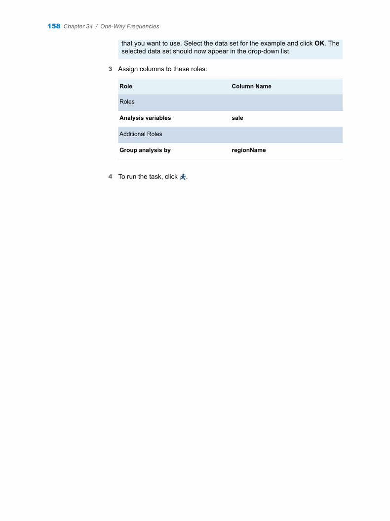
that you want to use. Select the data set for the example and click OK. The selected data set should now appear in the drop-down list.
3 Assign columns to these roles:
Role Column Name
Roles
Analysis variables sale
Additional Roles
Group analysis by regionName
4 To run the task, click .
158 Chapter 34 / One-Way Frequencies
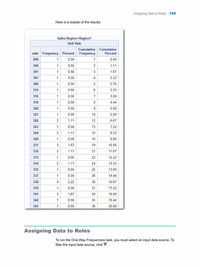
Here is a subset of the results:
Assigning Data to Roles
To run the One-Way Frequencies task, you must select an input data source. To filter the input data source, click .
Assigning Data to Roles 159
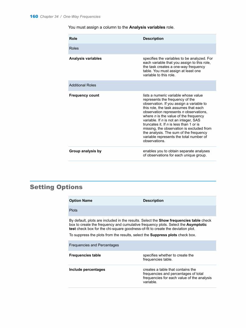
You must assign a column to the Analysis variables role.
Role Description
Roles
Analysis variables specifies the variables to be analyzed. For each variable that you assign to this role, the task creates a one-way frequency table. You must assign at least one variable to this role.
Additional Roles
Frequency count lists a numeric variable whose value represents the frequency of the observation. If you assign a variable to this role, the task assumes that each observation represents n observations, where n is the value of the frequency variable. If n is not an integer, SAS truncates it. If n is less than 1 or is missing, the observation is excluded from the analysis. The sum of the frequency variable represents the total number of observations.
Group analysis by enables you to obtain separate analyses of observations for each unique group.
Setting Options
Option Name Description
Plots
By default, plots are included in the results. Select the Show frequencies table check box to create the frequency and cumulative frequency plots. Select the Asymptotic test check box for the chi-square goodness-of-fit to create the deviation plot.
To suppress the plots from the results, select the Suppress plots check box.
Frequencies and Percentages
Frequencies table specifies whether to create the frequencies table.
Include percentages creates a table that contains the frequencies and percentages of total frequencies for each value of the analysis variable.
160 Chapter 34 / One-Way Frequencies
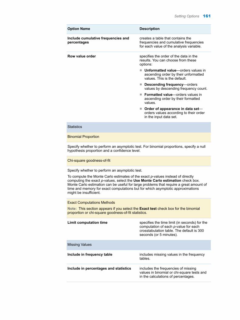
Option Name Description
Include cumulative frequencies and percentages
creates a table that contains the frequencies and cumulative frequencies for each value of the analysis variable.
Row value order specifies the order of the data in the results. You can choose from these options:n Unformatted value—orders values in
ascending order by their unformatted values. This is the default.
n Descending frequency—orders values by descending frequency count.
n Formatted value—orders values in ascending order by their formatted values.
n Order of appearance in data set—orders values according to their order in the input data set.
Statistics
Binomial Proportion
Specify whether to perform an asymptotic test. For binomial proportions, specify a null hypothesis proportion and a confidence level.
Chi-square goodness-of-fit
Specify whether to perform an asymptotic test.
To compute the Monte Carlo estimates of the exact p-values instead of directly computing the exact p-values, select the Use Monte Carlo estimation check box. Monte Carlo estimation can be useful for large problems that require a great amount of time and memory for exact computations but for which asymptotic approximations might be insufficient.
Exact Computations Methods
Note: This section appears if you select the Exact test check box for the binomial proportion or chi-square goodness-of-fit statistics.
Limit computation time specifies the time limit (in seconds) for the computation of each p-value for each crosstabulation table. The default is 300 seconds (or 5 minutes).
Missing Values
Include in frequency table includes missing values in the frequency tables.
Include in percentages and statistics includes the frequencies of missing values in binomial or chi-square tests and in the calculations of percentages.
Setting Options 161

162 Chapter 34 / One-Way Frequencies
35Correlation Analysis
About the Correlation Analysis Task . . . . . . . . . . . . . . . . . . . . . . . . . . . . . . . . . . . . . . . 163
Example: Correlations in the Sashelp.Cars Data Set . . . . . . . . . . . . . . . . . . . . . . . 163
Assigning Data to Roles . . . . . . . . . . . . . . . . . . . . . . . . . . . . . . . . . . . . . . . . . . . . . . . . . . . 164
Setting Options . . . . . . . . . . . . . . . . . . . . . . . . . . . . . . . . . . . . . . . . . . . . . . . . . . . . . . . . . . . . 165
Setting the Output Options . . . . . . . . . . . . . . . . . . . . . . . . . . . . . . . . . . . . . . . . . . . . . . . . 167
About the Correlation Analysis Task
Correlation is a statistical procedure for describing the relationship between numeric variables. The relationship is described by calculating correlation coefficients for the variables. The correlations range from –1 to 1. The Correlation Analysis task provides graphs and statistics for investigating associations among variables.
Note: You must license and install SAS/STAT to use this task.
Example: Correlations in the Sashelp.Cars Data Set
To create this example:
1 In the Tasks section, expand the Statistics folder, and then double-click Correlation Analysis. The user interface for the Correlation Analysis task opens.
2 On the Data tab, select the SASHELP.CARS data set.
TIP If the data set is not available from the drop-down list, click . In
the Choose a Table window, expand the library that contains the data set that you want to use. Select the data set for the example and click OK. The selected data set should now appear in the drop-down list.
3 Assign columns to these roles:
163
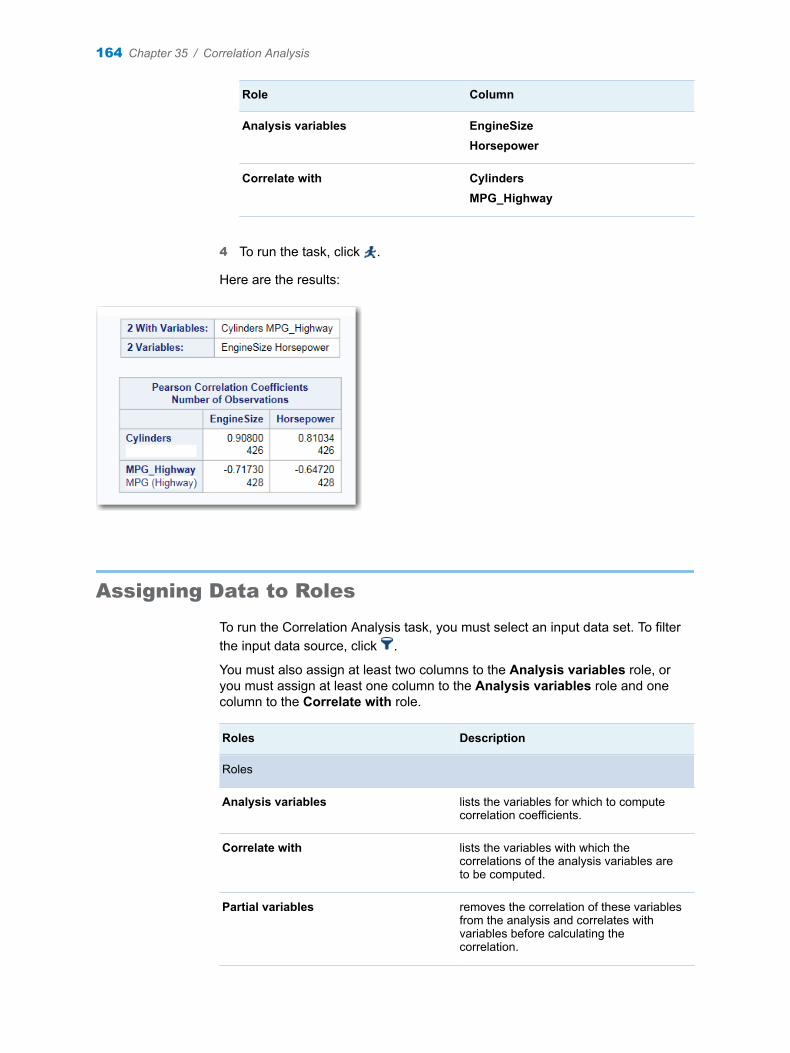
Role Column
Analysis variables EngineSizeHorsepower
Correlate with CylindersMPG_Highway
4 To run the task, click .
Here are the results:
Assigning Data to Roles
To run the Correlation Analysis task, you must select an input data set. To filter the input data source, click .
You must also assign at least two columns to the Analysis variables role, or you must assign at least one column to the Analysis variables role and one column to the Correlate with role.
Roles Description
Roles
Analysis variables lists the variables for which to compute correlation coefficients.
Correlate with lists the variables with which the correlations of the analysis variables are to be computed.
Partial variables removes the correlation of these variables from the analysis and correlates with variables before calculating the correlation.
164 Chapter 35 / Correlation Analysis
Roles Description
Additional Roles
Frequency count lists a numeric variable whose value represents the frequency of the observation. If you assign a variable to this role, the task assumes that each observation represents n observations, where n is the value of the frequency variable. If n is not an integer, SAS truncates it. If n is less than 1 or is missing, the observation is excluded from the analysis. The sum of the frequency variable represents the total number of observations.
Weight lists the weights to use in the calculation of Pearson weighted product-moment correlation.
Group analysis by enables you to obtain separate analyses of observations for each unique group.
Setting Options
Option Name Description
Methods
Missing values specifies how to treat observations with missing values. If you select the Use nonmissing values for all selected variables option, all observations with missing values are excluded from the analysis. If you select the Use nonmissing values for pairs of variables option, the correlation statistics are computed using the nonmissing pairs of variables.
Statistics
Setting Options 165
Option Name Description
By default, the results contain a table with the correlations and p-values. You can also include these statistics:
CorrelationsSelecting this option includes the correlations in the results. You can also specify probabilities that are associated with each correlation coefficient and whether to order the correlations from highest to lowest in absolute value.
CovariancesSelecting this option includes the variance and covariance matrix in the results. Also, the Pearson correlations are displayed. If you assign a column to the Partial variables role, the task computes a partial covariance matrix.
Sum of squares and cross-productsSelecting this option displays a table of the sums of squares and cross products in the results. The Pearson correlations are also included in the results. If you assign a column to the Partial variables role, the unpartial sums of squares and cross-products matrix is displayed.
Corrected sum of squares and cross-productsSelecting this option displays a table of the corrected sums of squares and cross products. The Pearson correlations are also included in the results. If you assign a column to the Partial variables role, the task computes both an unpartial and a partial corrected sum of squares and cross-products matrix.
Descriptive statisticsSelecting this option includes the simple descriptive statistics for each variable. Even if you do not select this option and you choose to create an output data set, the data set contains the descriptive statistics for the variables.
Fisher’s z transformationFor a Pearson correlation, you can use the Fisher transformation options to request confidence limits and p-values under a specified alternative (null) hypothesis, H0: ρ = ρ0, for correlation coefficients that use Fisher’s z transformation. If you select the Fisher’s z transformation check box, you must specify a value in the Null hypothesis box.
You can choose from these types of confidence limits:
n Two-sided confidence limits requests two-sided confidence limits for the test of the null hypothesis, H0: ρ = ρ0. This is the default.
n Lower confidence limit requests a lower confidence limit for the test of the one-sided null hypothesis, H0: ρ ≤ ρ0.
n Upper confidence limit requests an upper confidence limit for the test of the one-sided null hypothesis, H0: ρ ≥ ρ0.
By default, the level of the confidence limits for the correlation is 95%.
Nonparametric Correlations
Spearman’s rank-order correlation calculates Spearman rank-order correlation. This is a nonparametric measure of association that is based on the rank of the data values. The correlations range from –1 to 1.
166 Chapter 35 / Correlation Analysis
Option Name Description
Kendall’s tau-b calculates Kendall tau-b. This is a nonparametric measure of association that is based on the number of concordances and discordances in paired observations. Concordance occurs when paired observations vary together, and discordance occurs when paired observations vary differently. Kendall's tau-b ranges from –1 to 1.
Hoeffding’s measure of dependence calculates Hoeffding's measure of dependence, D. This is a nonparametric measure of association that detects more general departures from independence. This D statistic is 30 times larger than the usual definition and scales the range between –0.5 and 1 so that only large positive values indicate dependence.
Plots
You can include either of these plots in your results:n a scatter plot matrix for variables. You can also choose to include a histogram of the
analysis variables in the symmetric matrix plot.n a scatter plot for each applicable pair of distinct variables from the analysis
variables. You can specify whether to display the prediction ellipses for new observations or the confidence ellipses for the mean.
You can also specify the number of variables to plot and the maximum number of points to plot.
Setting the Output Options
You can specify whether to create an output data set that contains the Pearson correlation statistics. This data set also includes means, standard deviations, and the number of observations.
You can also choose to include these statistics in the output data set:
n Correlations – By default, the output data set contains the correlation coefficients with the corresponding _TYPE_ variable value of ‘CORR’.
n Covariances – When you select this option, the output data set contains the covariance matrix with the corresponding _TYPE_ variable value of ‘COV’.
n Sum of squares and cross-products – If you assign a column to the Partial variables role, the output data set does not contain a sum of squares and cross-products matrix.
n Corrected sum of squares and cross-products — If you assign a column to the Partial variables role, the output data set contains a partial corrected sum of squares and cross-products matrix.
Setting the Output Options 167

168 Chapter 35 / Correlation Analysis
36Table Analysis
About the Table Analysis Task . . . . . . . . . . . . . . . . . . . . . . . . . . . . . . . . . . . . . . . . . . . . . 169
Example: Distribution of Type by DriveTrain . . . . . . . . . . . . . . . . . . . . . . . . . . . . . . . 169
Assigning Data to Roles . . . . . . . . . . . . . . . . . . . . . . . . . . . . . . . . . . . . . . . . . . . . . . . . . . . 171
Setting Options . . . . . . . . . . . . . . . . . . . . . . . . . . . . . . . . . . . . . . . . . . . . . . . . . . . . . . . . . . . . 171
About the Table Analysis Task
The Table Analysis task provides one-way to n-way frequency and contingency (crosstabulation) tables. This task also generates statistics about the association between rows and columns.
Note: You must license and install SAS/STAT to use this task.
Example: Distribution of Type by DriveTrain
To create this example:
1 In the Tasks section, expand the Statistics folder, and then double-click Table Analysis. The user interface for the Table Analysis task opens.
2 On the Data tab, select the SASHELP.CARS data set.
TIP If the data set is not available from the drop-down list, click . In
the Choose a Table window, expand the library that contains the data set that you want to use. Select the data set for the example and click OK. The selected data set should now appear in the drop-down list.
3 Assign columns to these roles:
Role Column
Row variables Type
169

Role Column
Column variables DriveTrain
4 To run the task, click .
Here is a subset of the results:
170 Chapter 36 / Table Analysis
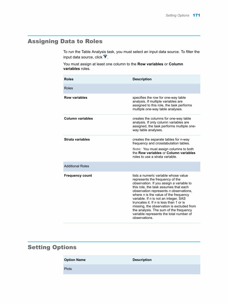
Assigning Data to Roles
To run the Table Analysis task, you must select an input data source. To filter the input data source, click .
You must assign at least one column to the Row variables or Column variables roles.
Roles Description
Roles
Row variables specifies the row for one-way table analysis. If multiple variables are assigned to this role, the task performs multiple one-way table analyses.
Column variables creates the columns for one-way table analysis. If only column variables are assigned, the task performs multiple one-way table analyses.
Strata variables creates the separate tables for n-way frequency and crosstabulation tables.
Note: You must assign columns to both the Row variables or Column variables roles to use a strata variable.
Additional Roles
Frequency count lists a numeric variable whose value represents the frequency of the observation. If you assign a variable to this role, the task assumes that each observation represents n observations, where n is the value of the frequency variable. If n is not an integer, SAS truncates it. If n is less than 1 or is missing, the observation is excluded from the analysis. The sum of the frequency variable represents the total number of observations.
Setting Options
Option Name Description
Plots
Setting Options 171
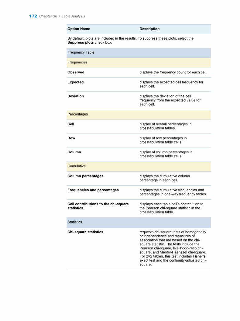
Option Name Description
By default, plots are included in the results. To suppress these plots, select the Suppress plots check box.
Frequency Table
Frequencies
Observed displays the frequency count for each cell.
Expected displays the expected cell frequency for each cell.
Deviation displays the deviation of the cell frequency from the expected value for each cell.
Percentages
Cell display of overall percentages in crosstabulation tables.
Row display of row percentages in crosstabulation table cells.
Column display of column percentages in crosstabulation table cells.
Cumulative
Column percentages displays the cumulative column percentage in each cell.
Frequencies and percentages displays the cumulative frequencies and percentages in one-way frequency tables.
Cell contributions to the chi-square statistics
displays each table cell’s contribution to the Pearson chi-square statistic in the crosstabulation table.
Statistics
Chi-square statistics requests chi-square tests of homogeneity or independence and measures of association that are based on the chi-square statistic. The tests include the Pearson chi-square, likelihood-ratio chi-square, and Mantel-Haenszel chi-square. For 2×2 tables, this test includes Fisher's exact test and the continuity-adjusted chi-square.
172 Chapter 36 / Table Analysis
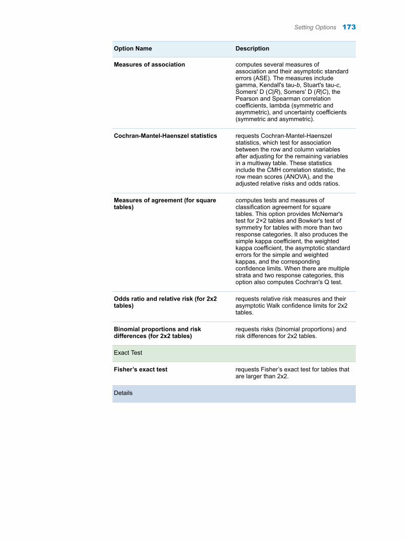
Option Name Description
Measures of association computes several measures of association and their asymptotic standard errors (ASE). The measures include gamma, Kendall's tau-b, Stuart's tau-c, Somers' D (C|R), Somers' D (R|C), the Pearson and Spearman correlation coefficients, lambda (symmetric and asymmetric), and uncertainty coefficients (symmetric and asymmetric).
Cochran-Mantel-Haenszel statistics requests Cochran-Mantel-Haenszel statistics, which test for association between the row and column variables after adjusting for the remaining variables in a multiway table. These statistics include the CMH correlation statistic, the row mean scores (ANOVA), and the adjusted relative risks and odds ratios.
Measures of agreement (for square tables)
computes tests and measures of classification agreement for square tables. This option provides McNemar's test for 2×2 tables and Bowker's test of symmetry for tables with more than two response categories. It also produces the simple kappa coefficient, the weighted kappa coefficient, the asymptotic standard errors for the simple and weighted kappas, and the corresponding confidence limits. When there are multiple strata and two response categories, this option also computes Cochran's Q test.
Odds ratio and relative risk (for 2x2 tables)
requests relative risk measures and their asymptotic Walk confidence limits for 2x2 tables.
Binomial proportions and risk differences (for 2x2 tables)
requests risks (binomial proportions) and risk differences for 2x2 tables.
Exact Test
Fisher’s exact test requests Fisher’s exact test for tables that are larger than 2x2.
Details
Setting Options 173
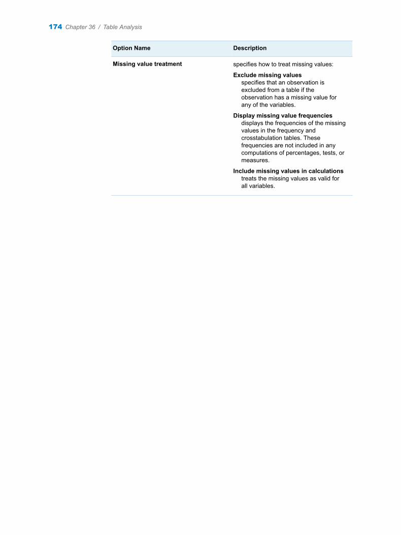
Option Name Description
Missing value treatment specifies how to treat missing values:
Exclude missing valuesspecifies that an observation is excluded from a table if the observation has a missing value for any of the variables.
Display missing value frequenciesdisplays the frequencies of the missing values in the frequency and crosstabulation tables. These frequencies are not included in any computations of percentages, tests, or measures.
Include missing values in calculationstreats the missing values as valid for all variables.
174 Chapter 36 / Table Analysis
37t Tests
About the t Tests Task . . . . . . . . . . . . . . . . . . . . . . . . . . . . . . . . . . . . . . . . . . . . . . . . . . . . . 175
One-Sample t Test . . . . . . . . . . . . . . . . . . . . . . . . . . . . . . . . . . . . . . . . . . . . . . . . . . . . . . . . . 176About the One-Sample t Test . . . . . . . . . . . . . . . . . . . . . . . . . . . . . . . . . . . . . . . . . . . . . 176Example: One-Sample t Test for Horsepower . . . . . . . . . . . . . . . . . . . . . . . . . . . . . . 176Assigning Data to Roles . . . . . . . . . . . . . . . . . . . . . . . . . . . . . . . . . . . . . . . . . . . . . . . . . 178Setting Options . . . . . . . . . . . . . . . . . . . . . . . . . . . . . . . . . . . . . . . . . . . . . . . . . . . . . . . . . 178
Paired Test . . . . . . . . . . . . . . . . . . . . . . . . . . . . . . . . . . . . . . . . . . . . . . . . . . . . . . . . . . . . . . . . 180About the Paired t Test . . . . . . . . . . . . . . . . . . . . . . . . . . . . . . . . . . . . . . . . . . . . . . . . . . 180Example: Determining the Distribution of Price – Cost . . . . . . . . . . . . . . . . . . . . . . 180Assigning Data to Roles . . . . . . . . . . . . . . . . . . . . . . . . . . . . . . . . . . . . . . . . . . . . . . . . . 182Setting Options . . . . . . . . . . . . . . . . . . . . . . . . . . . . . . . . . . . . . . . . . . . . . . . . . . . . . . . . . 182
Two-Sample t Test . . . . . . . . . . . . . . . . . . . . . . . . . . . . . . . . . . . . . . . . . . . . . . . . . . . . . . . . . 184About the Two-Sample t Test Task . . . . . . . . . . . . . . . . . . . . . . . . . . . . . . . . . . . . . . . . 184Example: Two-Sample t Test . . . . . . . . . . . . . . . . . . . . . . . . . . . . . . . . . . . . . . . . . . . . . 185Assigning Data to Roles . . . . . . . . . . . . . . . . . . . . . . . . . . . . . . . . . . . . . . . . . . . . . . . . . 187Setting Options . . . . . . . . . . . . . . . . . . . . . . . . . . . . . . . . . . . . . . . . . . . . . . . . . . . . . . . . . 187
About the t Tests Task
Using the t Tests task, you can perform a one-sample test, a paired test, or a two-sample test.
For more information, see these topics:
n “One-Sample t Test” on page 176
n “Paired Test” on page 180
n “Two-Sample t Test” on page 184
Note: You must license and install SAS/STAT to use this task.
175
One-Sample t Test
About the One-Sample t Test
A one-sample t test compares the mean of the sample to the null hypothesis mean.
To compare an individual mean with a sample size of n to a value m, use t = x − m
sn
where x is the sample mean of the observations and s2 is the sample
variance of the observations.
For example, you want to perform a one-sample t test on the horsepower values in the Sashelp.Cars data set. The null hypothesis is 300.
To run a one-sample t test, open the t Tests task. From the t test drop-down list, select One-sample test.
Example: One-Sample t Test for Horsepower
To create this example:
1 In the Tasks section, expand the Statistics folder, and then double-click t Tests. The user interface for the t Tests task opens.
2 On the Data tab, select the SASHELP.CARS data set.
TIP If the data set is not available from the drop-down list, click . In
the Choose a Table window, expand the library that contains the data set that you want to use. Select the data set for the example and click OK. The selected data set should now appear in the drop-down list.
3 From the t test drop-down list, select One-sample test.
4 To the Analysis variable role, assign the Horsepower column.
5 On the Options tab, enter 300 in the Alternative hypothesis field.
6 To run the task, click .
176 Chapter 37 / t Tests
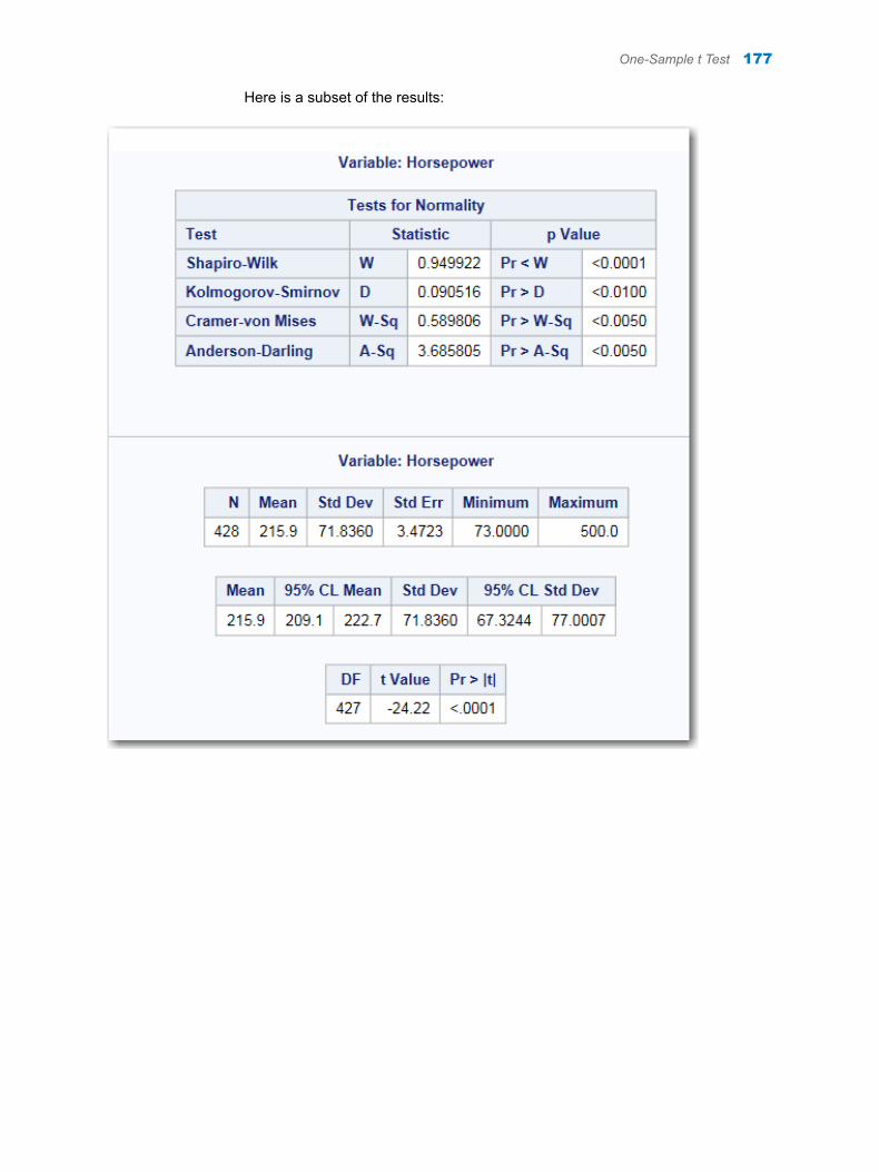
Here is a subset of the results:
One-Sample t Test 177
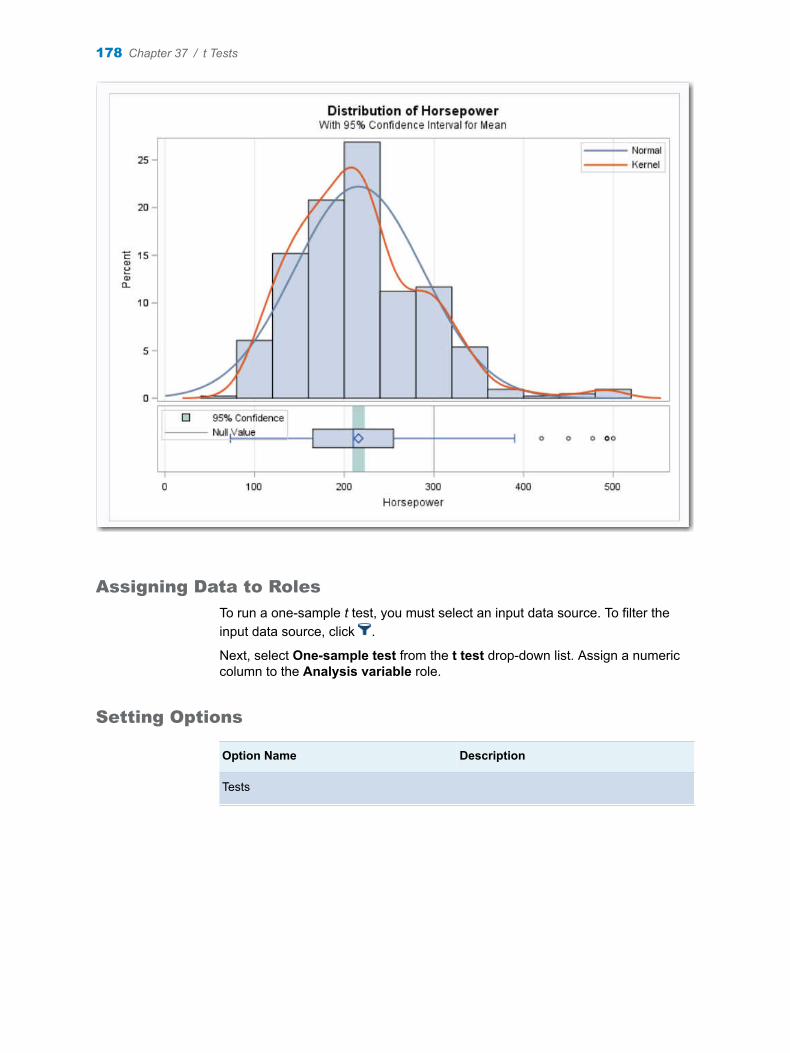
Assigning Data to Roles
To run a one-sample t test, you must select an input data source. To filter the input data source, click .
Next, select One-sample test from the t test drop-down list. Assign a numeric column to the Analysis variable role.
Setting Options
Option Name Description
Tests
178 Chapter 37 / t Tests
Option Name Description
Tails specifies the number of sides (or tails) and direction of the statistical tests and test-based confidence intervals. You can choose from these options:n Two-tailed test specifies two-sided
tests and confidence intervals for means.
n Upper one-tailed test specifies upper one-sided tests in which the alternative hypothesis indicates a mean greater than the null value, and upper one-sided confidence intervals between the lower confidence limit and infinity.
n Lower one-tailed test specifies lower one-sided tests in which the alternative hypothesis indicates a mean less than the null value, and lower one-sided confidence intervals between minus infinity and the upper confidence limit.
Alternative hypothesis specifies the value of the null hypothesis. By default, the null hypothesis has a value of 0.
Normality Assumption
Tests for normality runs tests for normality that include a series of goodness-of-fit tests based on the empirical distribution function. The table provides test statistics and p-values for the Shapiro-Wilk test (provided the sample size is less than or equal to 2000), the Kolmogorov-Smirnov test, the Anderson-Darling test, and the Cramér-von Mises test.
Nonparametric Tests
Note: This option is available only for a two-tailed test.
Sign test and Wilcoxon signed rank test
generates the results from these tests:n The sign test statistic is
M = n+ − n− /2 , where n+ is the number of values that are greater than μ0, and n- is the number of values that are less than μ0. Values equal to μ0are discarded.
n The Wilcoxon signed rank statistic S is calculated as
S = ∑i: xi − μ0 > 0
ri+ −
nt nt + 14 ,
where r+i is the rank of xi − μ0 after
discarding values of xi − μ0 , and nt is the number of xi values not equal to μ0. Average ranks are used for tied values.
One-Sample t Test 179
Option Name Description
Plots
Histogram and box plot creates a histogram and box plot together in a single panel, sharing common X axes.
Normality plot creates a normal quantile-quantile (Q-Q) plot.
Confidence interval plot creates a plot of the confidence interval for the means.
Paired Test
About the Paired t Test
A paired t test compares the mean of the differences in the observations to a given number, the null hypothesis difference. The paired t test is used when the two samples are correlated, such as two measures of blood pressure from the same person.
To compare n paired differences to a value m, use t = d − msd
n
, where d is the
sample mean of the paired differences and s2d is the sample variance of the
paired differences.
To run a paired t test, open the t Tests task. From the t test drop-down list, select Paired test.
Example: Determining the Distribution of Price – Cost
In this example, you want to compare the means of differences in price and cost in the Sashelp.Pricedata data set. The null hypothesis for this test is 30.
To create this example:
1 In the Tasks section, expand the Statistics folder, and then double-click t Tests. The user interface for the t Tests task opens.
2 On the Data tab, select the SASHELP.PRICEDATA data set.
TIP If the data set is not available from the drop-down list, click . In
the Choose a Table window, expand the library that contains the data set that you want to use. Select the data set for the example and click OK. The selected data set should now appear in the drop-down list.
180 Chapter 37 / t Tests
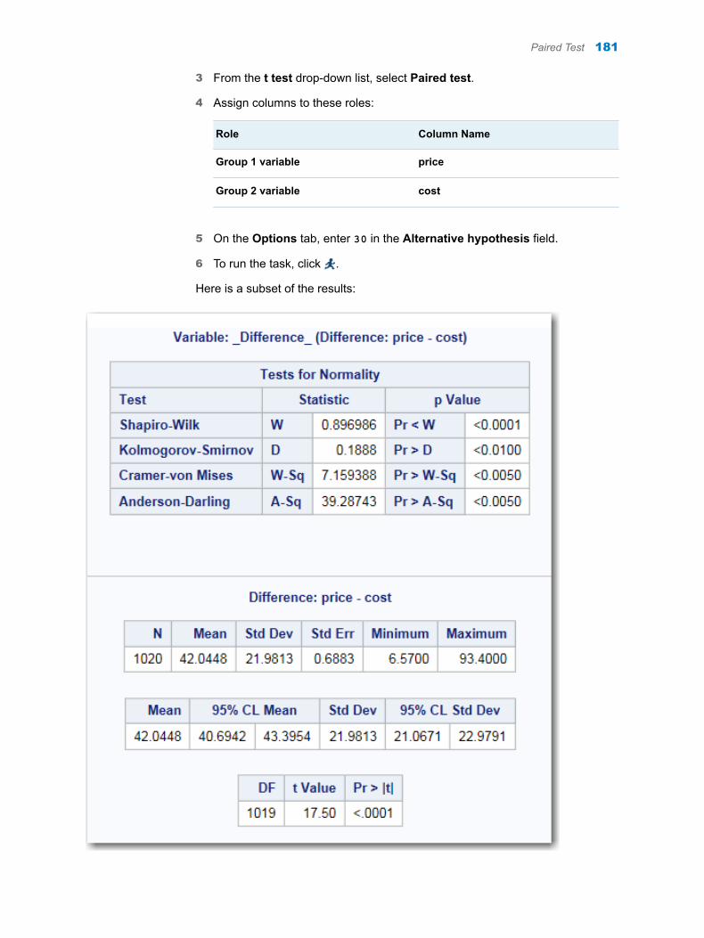
3 From the t test drop-down list, select Paired test.
4 Assign columns to these roles:
Role Column Name
Group 1 variable price
Group 2 variable cost
5 On the Options tab, enter 30 in the Alternative hypothesis field.
6 To run the task, click .
Here is a subset of the results:
Paired Test 181
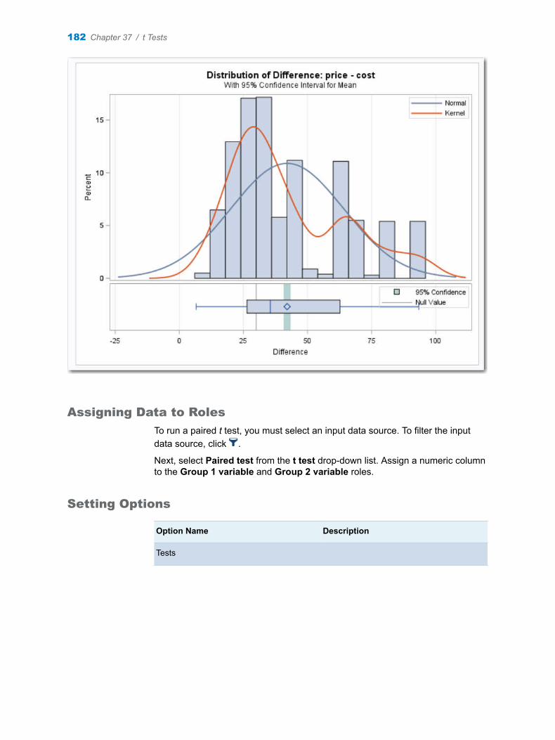
Assigning Data to Roles
To run a paired t test, you must select an input data source. To filter the input data source, click .
Next, select Paired test from the t test drop-down list. Assign a numeric column to the Group 1 variable and Group 2 variable roles.
Setting Options
Option Name Description
Tests
182 Chapter 37 / t Tests
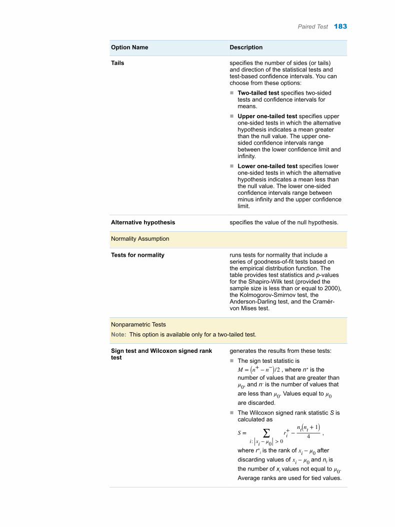
Option Name Description
Tails specifies the number of sides (or tails) and direction of the statistical tests and test-based confidence intervals. You can choose from these options:n Two-tailed test specifies two-sided
tests and confidence intervals for means.
n Upper one-tailed test specifies upper one-sided tests in which the alternative hypothesis indicates a mean greater than the null value. The upper one-sided confidence intervals range between the lower confidence limit and infinity.
n Lower one-tailed test specifies lower one-sided tests in which the alternative hypothesis indicates a mean less than the null value. The lower one-sided confidence intervals range between minus infinity and the upper confidence limit.
Alternative hypothesis specifies the value of the null hypothesis.
Normality Assumption
Tests for normality runs tests for normality that include a series of goodness-of-fit tests based on the empirical distribution function. The table provides test statistics and p-values for the Shapiro-Wilk test (provided the sample size is less than or equal to 2000), the Kolmogorov-Smirnov test, the Anderson-Darling test, and the Cramér-von Mises test.
Nonparametric Tests
Note: This option is available only for a two-tailed test.
Sign test and Wilcoxon signed rank test
generates the results from these tests:n The sign test statistic is
M = n+ − n− /2 , where n+ is the number of values that are greater than μ0, and n- is the number of values that are less than μ0. Values equal to μ0are discarded.
n The Wilcoxon signed rank statistic S is calculated as
S = ∑i: xi − μ0 > 0
ri+ −
nt nt + 14 ,
where r+i is the rank of xi − μ0 after
discarding values of xi − μ0 and nt is the number of xi values not equal to μ0. Average ranks are used for tied values.
Paired Test 183
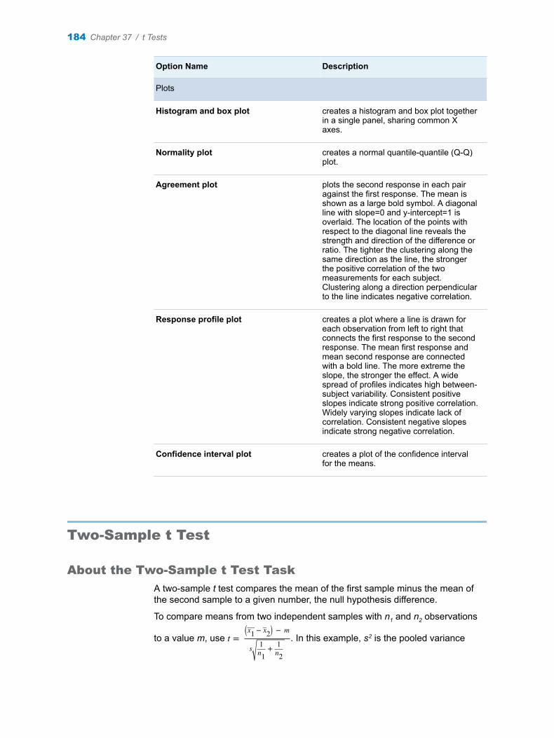
Option Name Description
Plots
Histogram and box plot creates a histogram and box plot together in a single panel, sharing common X axes.
Normality plot creates a normal quantile-quantile (Q-Q) plot.
Agreement plot plots the second response in each pair against the first response. The mean is shown as a large bold symbol. A diagonal line with slope=0 and y-intercept=1 is overlaid. The location of the points with respect to the diagonal line reveals the strength and direction of the difference or ratio. The tighter the clustering along the same direction as the line, the stronger the positive correlation of the two measurements for each subject. Clustering along a direction perpendicular to the line indicates negative correlation.
Response profile plot creates a plot where a line is drawn for each observation from left to right that connects the first response to the second response. The mean first response and mean second response are connected with a bold line. The more extreme the slope, the stronger the effect. A wide spread of profiles indicates high between-subject variability. Consistent positive slopes indicate strong positive correlation. Widely varying slopes indicate lack of correlation. Consistent negative slopes indicate strong negative correlation.
Confidence interval plot creates a plot of the confidence interval for the means.
Two-Sample t Test
About the Two-Sample t Test Task
A two-sample t test compares the mean of the first sample minus the mean of the second sample to a given number, the null hypothesis difference.
To compare means from two independent samples with n1 and n2 observations
to a value m, use t =x1 − x2 − m
s 1n1
+ 1n2
. In this example, s2 is the pooled variance
184 Chapter 37 / t Tests
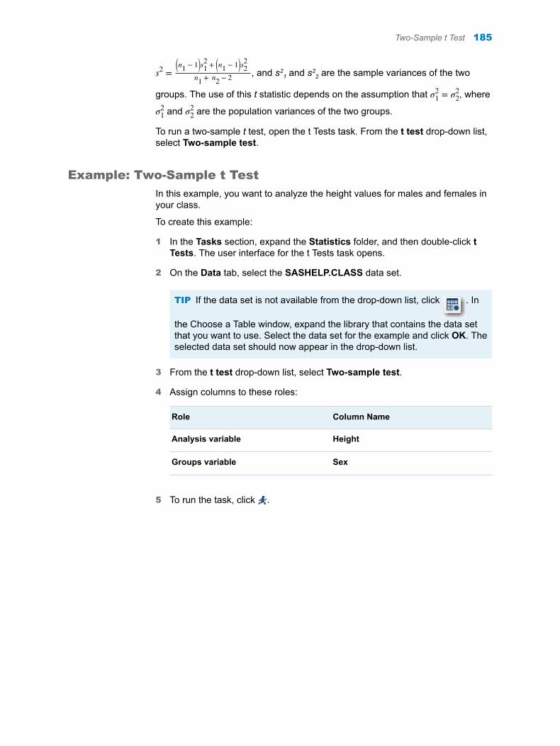
s2 =n1 − 1 s1
2 + n1 − 1 s22
n1 + n2 − 2 , and s21 and s2
2 are the sample variances of the two
groups. The use of this t statistic depends on the assumption that σ12 = σ2
2, where
σ12 and σ2
2 are the population variances of the two groups.
To run a two-sample t test, open the t Tests task. From the t test drop-down list, select Two-sample test.
Example: Two-Sample t Test
In this example, you want to analyze the height values for males and females in your class.
To create this example:
1 In the Tasks section, expand the Statistics folder, and then double-click t Tests. The user interface for the t Tests task opens.
2 On the Data tab, select the SASHELP.CLASS data set.
TIP If the data set is not available from the drop-down list, click . In
the Choose a Table window, expand the library that contains the data set that you want to use. Select the data set for the example and click OK. The selected data set should now appear in the drop-down list.
3 From the t test drop-down list, select Two-sample test.
4 Assign columns to these roles:
Role Column Name
Analysis variable Height
Groups variable Sex
5 To run the task, click .
Two-Sample t Test 185
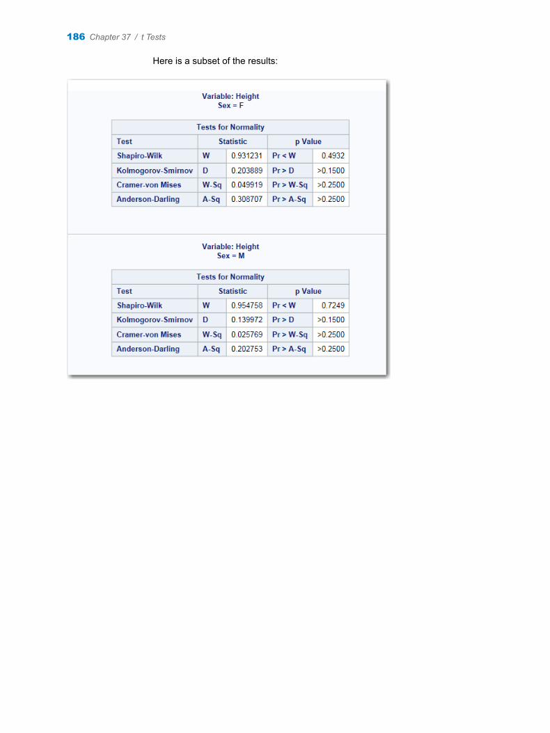
Here is a subset of the results:
186 Chapter 37 / t Tests
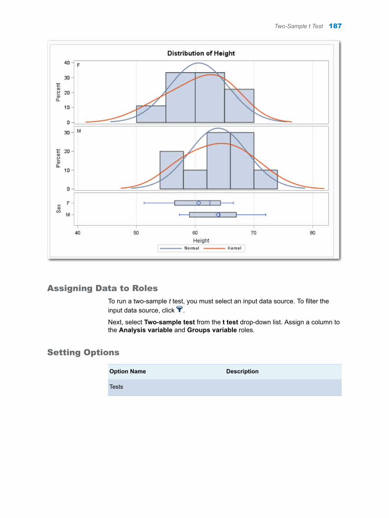
Assigning Data to Roles
To run a two-sample t test, you must select an input data source. To filter the input data source, click .
Next, select Two-sample test from the t test drop-down list. Assign a column to the Analysis variable and Groups variable roles.
Setting Options
Option Name Description
Tests
Two-Sample t Test 187
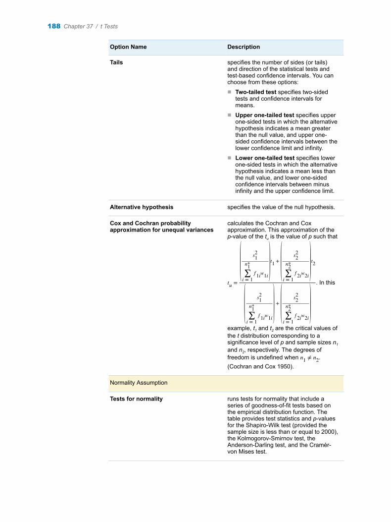
Option Name Description
Tails specifies the number of sides (or tails) and direction of the statistical tests and test-based confidence intervals. You can choose from these options:n Two-tailed test specifies two-sided
tests and confidence intervals for means.
n Upper one-tailed test specifies upper one-sided tests in which the alternative hypothesis indicates a mean greater than the null value, and upper one-sided confidence intervals between the lower confidence limit and infinity.
n Lower one-tailed test specifies lower one-sided tests in which the alternative hypothesis indicates a mean less than the null value, and lower one-sided confidence intervals between minus infinity and the upper confidence limit.
Alternative hypothesis specifies the value of the null hypothesis.
Cox and Cochran probability approximation for unequal variances
calculates the Cochran and Cox approximation. This approximation of the p-value of the tu is the value of p such that
tu =
s12
∑i = 1
n1*f 1iw1i
t1 +s22
∑i = 1
n2*f 2iw2i
t2
s12
∑i = 1
n1*f 1iw1i
+s22
∑i = 1
n2*f 2iw2i
. In this
example, t1 and t2 are the critical values of the t distribution corresponding to a significance level of p and sample sizes n1
and n2, respectively. The degrees of freedom is undefined when n1 ≠ n2. (Cochran and Cox 1950).
Normality Assumption
Tests for normality runs tests for normality that include a series of goodness-of-fit tests based on the empirical distribution function. The table provides test statistics and p-values for the Shapiro-Wilk test (provided the sample size is less than or equal to 2000), the Kolmogorov-Smirnov test, the Anderson-Darling test, and the Cramér-von Mises test.
188 Chapter 37 / t Tests
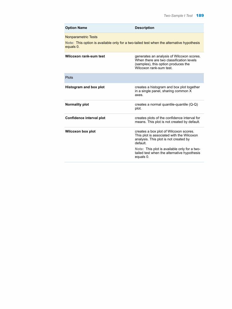
Option Name Description
Nonparametric Tests
Note: This option is available only for a two-tailed test when the alternative hypothesis equals 0.
Wilcoxon rank-sum test generates an analysis of Wilcoxon scores. When there are two classification levels (samples), this option produces the Wilcoxon rank-sum test.
Plots
Histogram and box plot creates a histogram and box plot together in a single panel, sharing common X axes.
Normality plot creates a normal quantile-quantile (Q-Q) plot.
Confidence interval plot creates plots of the confidence interval for means. This plot is not created by default.
Wilcoxon box plot creates a box plot of Wilcoxon scores. This plot is associated with the Wilcoxon analysis. This plot is not created by default.
Note: This plot is available only for a two-tailed test when the alternative hypothesis equals 0.
Two-Sample t Test 189

190 Chapter 37 / t Tests
38One-Way ANOVA
About the One-Way ANOVA Task . . . . . . . . . . . . . . . . . . . . . . . . . . . . . . . . . . . . . . . . . . 191
Example: Testing for Differences in the Means for MPG_Highway by Car Type . . . . . . . . . . . . . . . . . . . . . . . . . . . . . . . . . . . . . . . . . . . . . . . . 191
Assigning Data to Roles . . . . . . . . . . . . . . . . . . . . . . . . . . . . . . . . . . . . . . . . . . . . . . . . . . . 194
Setting Options . . . . . . . . . . . . . . . . . . . . . . . . . . . . . . . . . . . . . . . . . . . . . . . . . . . . . . . . . . . . 195
Setting the Output Options . . . . . . . . . . . . . . . . . . . . . . . . . . . . . . . . . . . . . . . . . . . . . . . . 197
About the One-Way ANOVA Task
The one-way analysis of variance (ANOVA) task tests and provides graphs for differences among the means of a single categorical variable on a single continuous dependent variable.
You might use the One-Way ANOVA task to do the following:
n study the effect of bacteria on the nitrogen content of red clover plants. The factor is the bacteria strain, and it has six levels.
n compare the life spans of three different brands of batteries. The factor is the brand, and it has three levels.
Note: You must license and install SAS/STAT to use this task.
Example: Testing for Differences in the Means for MPG_Highway by Car Type
In this example, you want to study the differences in the means for the number of highway miles per gallon for six car types.
To create this example:
1 In the Tasks section, expand the Statistics folder, and then double-click One-Way ANOVA. The user interface for the One-Way ANOVA task opens.
2 On the Data tab, select the SASHELP.CARS data set.
191
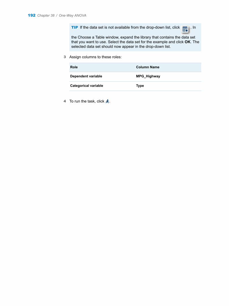
TIP If the data set is not available from the drop-down list, click . In
the Choose a Table window, expand the library that contains the data set that you want to use. Select the data set for the example and click OK. The selected data set should now appear in the drop-down list.
3 Assign columns to these roles:
Role Column Name
Dependent variable MPG_Highway
Categorical variable Type
4 To run the task, click .
192 Chapter 38 / One-Way ANOVA
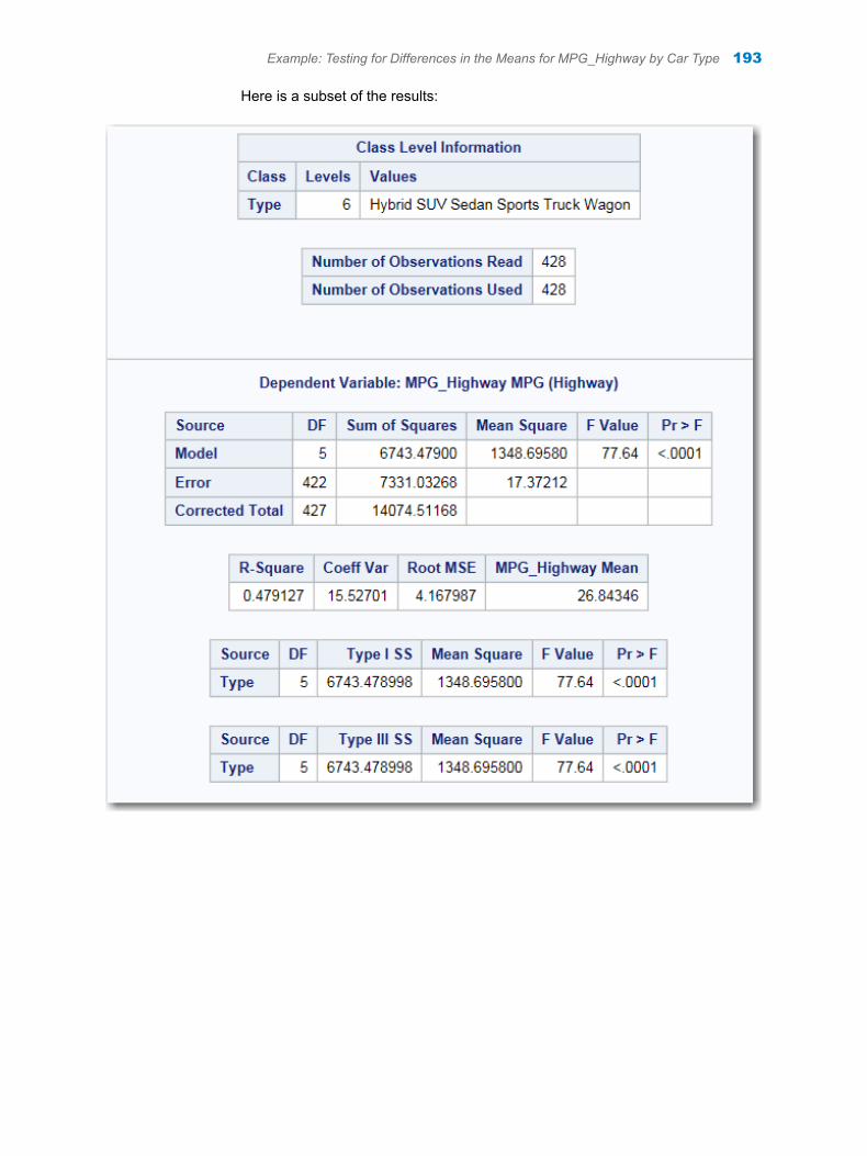
Here is a subset of the results:
Example: Testing for Differences in the Means for MPG_Highway by Car Type 193
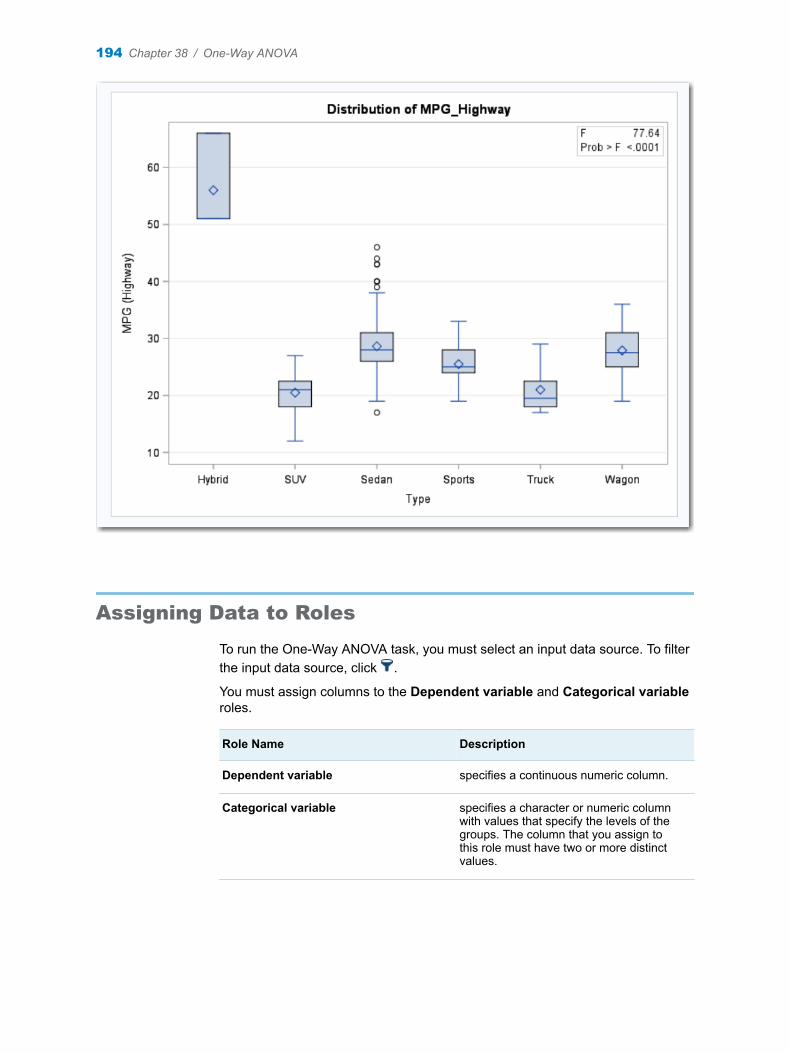
Assigning Data to Roles
To run the One-Way ANOVA task, you must select an input data source. To filter the input data source, click .
You must assign columns to the Dependent variable and Categorical variable roles.
Role Name Description
Dependent variable specifies a continuous numeric column.
Categorical variable specifies a character or numeric column with values that specify the levels of the groups. The column that you assign to this role must have two or more distinct values.
194 Chapter 38 / One-Way ANOVA
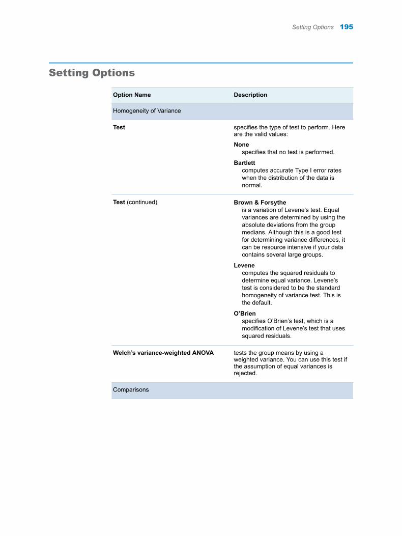
Setting Options
Option Name Description
Homogeneity of Variance
Test specifies the type of test to perform. Here are the valid values:
Nonespecifies that no test is performed.
Bartlettcomputes accurate Type I error rates when the distribution of the data is normal.
Test (continued) Brown & Forsytheis a variation of Levene's test. Equal variances are determined by using the absolute deviations from the group medians. Although this is a good test for determining variance differences, it can be resource intensive if your data contains several large groups.
Levenecomputes the squared residuals to determine equal variance. Levene’s test is considered to be the standard homogeneity of variance test. This is the default.
O’Brienspecifies O’Brien’s test, which is a modification of Levene’s test that uses squared residuals.
Welch’s variance-weighted ANOVA tests the group means by using a weighted variance. You can use this test if the assumption of equal variances is rejected.
Comparisons
Setting Options 195
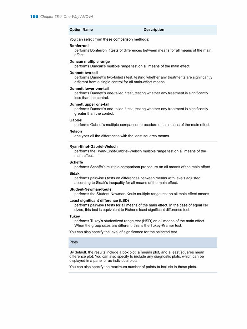
Option Name Description
You can select from these comparison methods:
Bonferroniperforms Bonferroni t tests of differences between means for all means of the main effect.
Duncan multiple rangeperforms Duncan’s multiple range test on all means of the main effect.
Dunnett two-tailperforms Dunnett’s two-tailed t test, testing whether any treatments are significantly different from a single control for all main-effect means.
Dunnett lower one-tailperforms Dunnett’s one-tailed t test, testing whether any treatment is significantly less than the control.
Dunnett upper one-tailperforms Dunnett’s one-tailed t test, testing whether any treatment is significantly greater than the control.
Gabrielperforms Gabriel’s multiple-comparison procedure on all means of the main effect.
Nelsonanalyzes all the differences with the least squares means.
Ryan-Einot-Gabriel-Welschperforms the Ryan-Einot-Gabriel-Welsch multiple range test on all means of the main effect.
Schefféperforms Scheffé’s multiple-comparison procedure on all means of the main effect.
Sidakperforms pairwise t tests on differences between means with levels adjusted according to Sidak’s inequality for all means of the main effect.
Student-Newman-Keulsperforms the Student-Newman-Keuls multiple range test on all main effect means.
Least significant difference (LSD)performs pairwise t tests for all means of the main effect. In the case of equal cell sizes, this test is equivalent to Fisher’s least significant difference test.
Tukeyperforms Tukey’s studentized range test (HSD) on all means of the main effect. When the group sizes are different, this is the Tukey-Kramer test.
You can also specify the level of significance for the selected test.
Plots
By default, the results include a box plot, a means plot, and a least squares mean difference plot. You can also specify to include any diagnostic plots, which can be displayed in a panel or as individual plots.
You can also specify the maximum number of points to include in these plots.
196 Chapter 38 / One-Way ANOVA

Setting the Output Options
You can specify whether to create an output data set. You can also specify the values to include in the output data set. You can include predicted values, residuals, standard errors, and influence statistics.
Setting the Output Options 197

198 Chapter 38 / One-Way ANOVA
39Nonparametric One-Way ANOVA
About the Nonparametric One-Way ANOVA Task . . . . . . . . . . . . . . . . . . . . . . . . . . 199
Example: Wilcoxon Scores for MPG_Highway Classified by Origin . . . . . . . . . 199
Assigning Data to Roles . . . . . . . . . . . . . . . . . . . . . . . . . . . . . . . . . . . . . . . . . . . . . . . . . . . 201
Setting Options . . . . . . . . . . . . . . . . . . . . . . . . . . . . . . . . . . . . . . . . . . . . . . . . . . . . . . . . . . . . 202
Creating an Output Data Set . . . . . . . . . . . . . . . . . . . . . . . . . . . . . . . . . . . . . . . . . . . . . . . 204
About the Nonparametric One-Way ANOVA Task
The Nonparametric One-Way ANOVA task consists of nonparametric tests for location and scale differences across a one-way classification. The task also provides a standard analysis of variance on the raw data and statistics based on the empirical distribution function.
Note: You must license and install SAS/STAT to use this task.
Example: Wilcoxon Scores for MPG_Highway Classified by Origin
To create this example:
1 In the Tasks section, expand the Statistics folder, and then double-click Nonparametric One-Way ANOVA. The user interface for the Nonparametric One-Way ANOVA task opens.
2 On the Data tab, select the SASHELP.CARS data set.
TIP If the data set is not available from the drop-down list, click . In
the Choose a Table window, expand the library that contains the data set that you want to use. Select the data set for the example and click OK. The selected data set should now appear in the drop-down list.
199
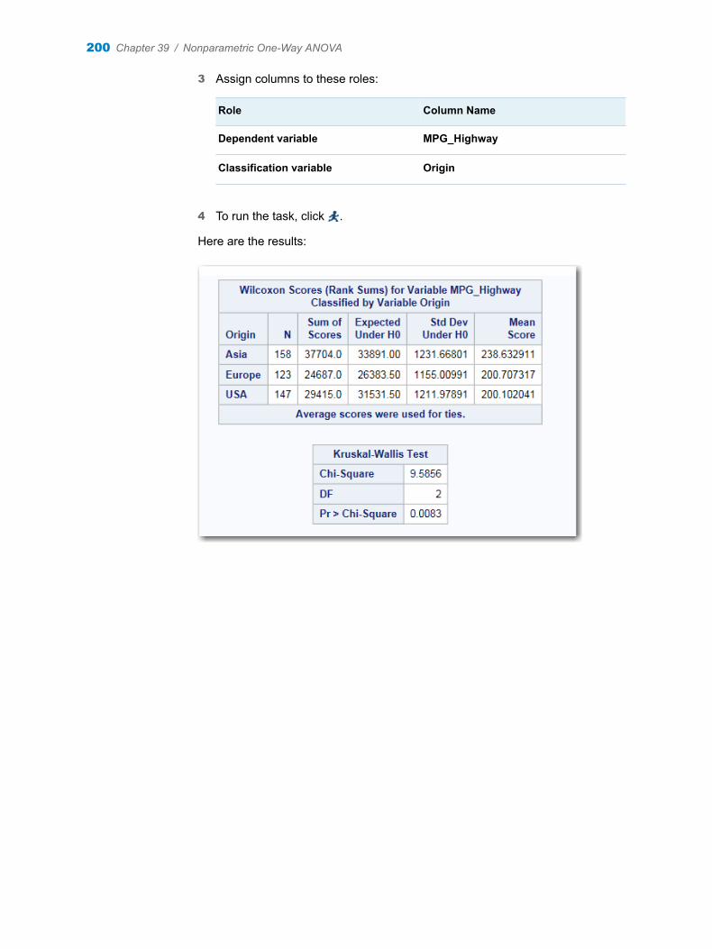
3 Assign columns to these roles:
Role Column Name
Dependent variable MPG_Highway
Classification variable Origin
4 To run the task, click .
Here are the results:
200 Chapter 39 / Nonparametric One-Way ANOVA
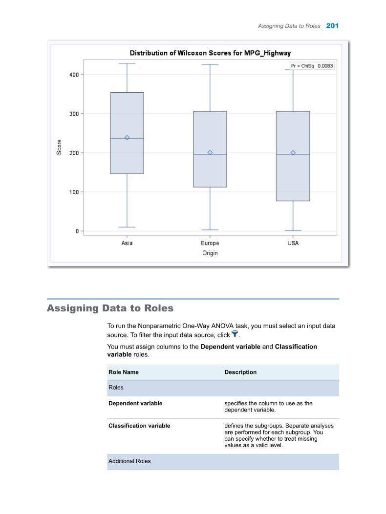
Assigning Data to Roles
To run the Nonparametric One-Way ANOVA task, you must select an input data source. To filter the input data source, click .
You must assign columns to the Dependent variable and Classification variable roles.
Role Name Description
Roles
Dependent variable specifies the column to use as the dependent variable.
Classification variable defines the subgroups. Separate analyses are performed for each subgroup. You can specify whether to treat missing values as a valid level.
Additional Roles
Assigning Data to Roles 201

Role Name Description
Frequency count lists a numeric variable whose value represents the frequency of the observation. If you assign a variable to this role, the task assumes that each observation represents n observations, where n is the value of the frequency variable. If n is not an integer, SAS truncates it. If n is less than 1 or is missing, the observation is excluded from the analysis. The sum of the frequency variable represents the total number of observations.
Group analysis by enables you to obtain separate analyses of observations for each unique group.
Setting Options
Option Name Description
Plots
By default, plots are included in the results. These plots are determined by the options that you select. Here are some of the plots that you can create:n By selecting the options in the Location Differences section, you can create a box
plot of Wilcoxon scores, a stacked bar chart showing frequencies above or below the overall median, a box plot of Van der Waerden scores, and a box plot of Savage scores.
n By selecting the options in the Scale Differences section, you can create a box plot of Ansari-Bradley scores, a box plot of Klotz scores, a box plot of Mood scores, and a box plot of Siegel-Tukey scores.
n By selecting the options in the Location and Scale Differences section, you can create a box plot of Conover scores.
n By selecting the Empirical distribution function tests, including Kolmogorov-Smirnov and Cramer-von Mises tests option, you can create a plot of the empirical distribution test.
You can specify whether to display the p-values in the plot.
To suppress the plots from the results, select the Suppress plots check box.
Tests
Tests specifies whether to calculate only the asymptotic tests or both the asymptotic tests and exact tests for the various analyses.
Location Differences
Wilcoxon scores
ranks of the observations.
Median scores equals 1 for observations greater than the median and 0 otherwise.
202 Chapter 39 / Nonparametric One-Way ANOVA
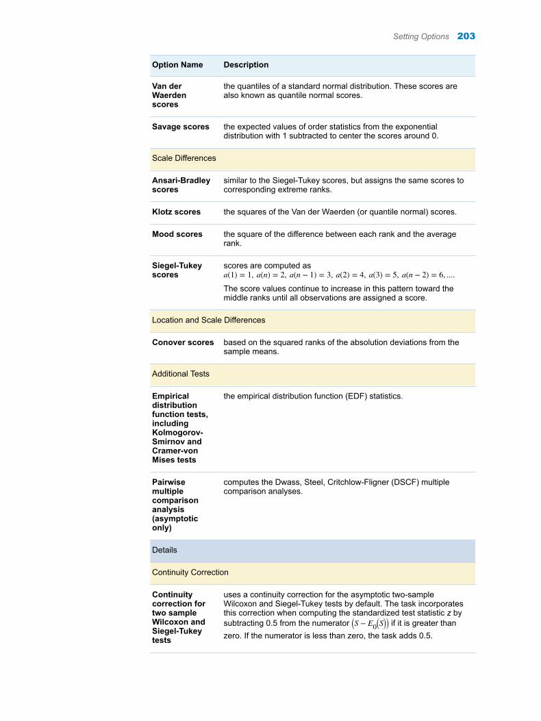
Option Name Description
Van der Waerden scores
the quantiles of a standard normal distribution. These scores are also known as quantile normal scores.
Savage scores the expected values of order statistics from the exponential distribution with 1 subtracted to center the scores around 0.
Scale Differences
Ansari-Bradley scores
similar to the Siegel-Tukey scores, but assigns the same scores to corresponding extreme ranks.
Klotz scores the squares of the Van der Waerden (or quantile normal) scores.
Mood scores the square of the difference between each rank and the average rank.
Siegel-Tukey scores
scores are computed as a 1 = 1, a n = 2, a n − 1 = 3, a 2 = 4, a 3 = 5, a n − 2 = 6, ....The score values continue to increase in this pattern toward the middle ranks until all observations are assigned a score.
Location and Scale Differences
Conover scores based on the squared ranks of the absolution deviations from the sample means.
Additional Tests
Empirical distribution function tests, including Kolmogorov-Smirnov and Cramer-von Mises tests
the empirical distribution function (EDF) statistics.
Pairwise multiple comparison analysis (asymptotic only)
computes the Dwass, Steel, Critchlow-Fligner (DSCF) multiple comparison analyses.
Details
Continuity Correction
Continuity correction for two sample Wilcoxon and Siegel-Tukey tests
uses a continuity correction for the asymptotic two-sample Wilcoxon and Siegel-Tukey tests by default. The task incorporates this correction when computing the standardized test statistic z by subtracting 0.5 from the numerator S − E0 S if it is greater than zero. If the numerator is less than zero, the task adds 0.5.
Setting Options 203
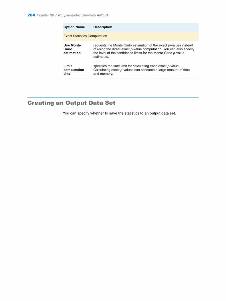
Option Name Description
Exact Statistics Computation
Use Monte Carlo estimation
requests the Monte Carlo estimation of the exact p-values instead of using the direct exact p-value computation. You can also specify the level of the confidence limits for the Monte Carlo p-value estimates.
Limit computation time
specifies the time limit for calculating each exact p-value. Calculating exact p-values can consume a large amount of time and memory.
Creating an Output Data Set
You can specify whether to save the statistics to an output data set.
204 Chapter 39 / Nonparametric One-Way ANOVA
40N-Way ANOVA
About the N-Way ANOVA Task . . . . . . . . . . . . . . . . . . . . . . . . . . . . . . . . . . . . . . . . . . . . . 205
Example: Analyzing the Sashelp.RevHub2 Data Set . . . . . . . . . . . . . . . . . . . . . . . . 205
Assigning Data to Roles . . . . . . . . . . . . . . . . . . . . . . . . . . . . . . . . . . . . . . . . . . . . . . . . . . . 207
Building a Model . . . . . . . . . . . . . . . . . . . . . . . . . . . . . . . . . . . . . . . . . . . . . . . . . . . . . . . . . . 207Requirements for Building a Model . . . . . . . . . . . . . . . . . . . . . . . . . . . . . . . . . . . . . . . 207Create a Main Effect . . . . . . . . . . . . . . . . . . . . . . . . . . . . . . . . . . . . . . . . . . . . . . . . . . . . . 208Create Crossed Effects (Interactions) . . . . . . . . . . . . . . . . . . . . . . . . . . . . . . . . . . . . . 208Create a Nested Effect . . . . . . . . . . . . . . . . . . . . . . . . . . . . . . . . . . . . . . . . . . . . . . . . . . . 208Create a Full Factorial Model . . . . . . . . . . . . . . . . . . . . . . . . . . . . . . . . . . . . . . . . . . . . . 208Create an N-Way Factorial . . . . . . . . . . . . . . . . . . . . . . . . . . . . . . . . . . . . . . . . . . . . . . . 208
Setting Options . . . . . . . . . . . . . . . . . . . . . . . . . . . . . . . . . . . . . . . . . . . . . . . . . . . . . . . . . . . . 209
Setting the Output Options . . . . . . . . . . . . . . . . . . . . . . . . . . . . . . . . . . . . . . . . . . . . . . . . 209
About the N-Way ANOVA Task
The N-Way ANOVA task tests and provides graphs for effects of one or more factors on the means of a single, continuous dependent variable.
Note: You must license and install SAS/STAT to use this task.
Example: Analyzing the Sashelp.RevHub2 Data Set
To create this example:
1 In the Tasks section, expand the Statistics folder, and then double-click N-Way ANOVA. The user interface for the N-Way ANOVA task opens.
2 On the Data tab, select the SASHELP.REVHUB2 data set.
TIP If the data set is not available from the drop-down list, click . In
the Choose a Table window, expand the library that contains the data set
205
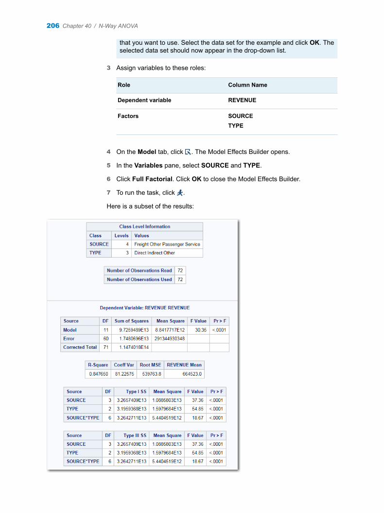
that you want to use. Select the data set for the example and click OK. The selected data set should now appear in the drop-down list.
3 Assign variables to these roles:
Role Column Name
Dependent variable REVENUE
Factors SOURCETYPE
4 On the Model tab, click . The Model Effects Builder opens.
5 In the Variables pane, select SOURCE and TYPE.
6 Click Full Factorial. Click OK to close the Model Effects Builder.
7 To run the task, click .
Here is a subset of the results:
206 Chapter 40 / N-Way ANOVA
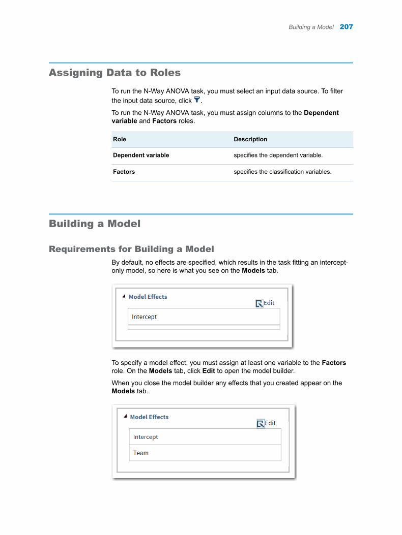
Assigning Data to Roles
To run the N-Way ANOVA task, you must select an input data source. To filter the input data source, click .
To run the N-Way ANOVA task, you must assign columns to the Dependent variable and Factors roles.
Role Description
Dependent variable specifies the dependent variable.
Factors specifies the classification variables.
Building a Model
Requirements for Building a Model
By default, no effects are specified, which results in the task fitting an intercept-only model, so here is what you see on the Models tab.
To specify a model effect, you must assign at least one variable to the Factors role. On the Models tab, click Edit to open the model builder.
When you close the model builder any effects that you created appear on the Models tab.
Building a Model 207
Create a Main Effect
1 Select the variable name in the Variables box.
2 Click Add to add the variable to the list of model effects.
Create Crossed Effects (Interactions)
1 Select two or more variables in the Variables box. To select more than one variable, press Ctrl.
2 Click Cross.
Create a Nested Effect
Nested effects are specified by following a main effect or crossed effect with a classification variable or list of classification variables enclosed in parentheses. Here are examples of nested effects: B(A), C(B*A), D*E(C*B*A). In this example, B(A) is read "B within A."
1 Select the classification variable in the Model Effects Builder.
2 Click Nest. The Nested window appears.
3 Select the variable to use in the nested effect. Click Outer or Nested within Outer to specify how to create the nested effect.
Note: The Nested within Outer button is available only when a classification variable is selected.
4 Select the effect that you want to nest.
5 Click Add.
Create a Full Factorial Model
1 Select two or more variables in the Variables box.
2 Click Full Factorial.
For example, if you select the Height, Weight, and Age variables and then click Full Factorial, these model effects are created: Age, Height, Weight, Age*Height, Age*Weight, Height*Weight, and Age*Height*Weight.
Create an N-Way Factorial
1 Select two or more variables in the Variables box.
2 Click N-way Factorial and specify the value of N.
For example, if you select the Height, Weight, and Age variables, click N-way Factorial, and then specify the value of N as 2, these model effects are created:
208 Chapter 40 / N-Way ANOVA

Age, Height, Weight, Age*Height, Age*Weight, and Height*Weight. If N is set to a value greater than the number of variables in the model, N is effectively set to the number of variables.
Setting Options
Option Description
Statistics
You can choose to display only the default statistics, the default statistics and additional statistics, or no statistics in the output.
Here are the options for the additional statistics:
n Perform multiple comparisons computes the least squares means for the specified effects. You can specify the method for adjustments for the p-values and confidence limits for the differences of the least squares means.
n The Sum of Squares options enable you to display the sum of squares associated with Type I estimable functions for each effect and the sum of squares associated with Type III estimable functions for each effect.
Plots
You can choose to display only the default plots, only selected plots, or no plots in your output. You can specify the maximum number of points to display in the plots.
Here are some plots that you can include in your results:
n least squares means plotn mean difference plotn interaction plot (available only if there are two variables assigned to the Factors
role)n analysis of means plot (available only if you select the Nelson method for
adjustment)n diagnostic plots, which can be displayed individually or in a panel
Setting the Output Options
You can specify whether to create an output data set. You can also specify the values to include in the output data set. You can include predicted values, residuals, standard errors, and influence statistics.
Setting the Output Options 209

210 Chapter 40 / N-Way ANOVA
41Analysis of Covariance
About the Analysis of Covariance Task . . . . . . . . . . . . . . . . . . . . . . . . . . . . . . . . . . . . 211
Example: Analyzing the Sashelp.Class Data Set . . . . . . . . . . . . . . . . . . . . . . . . . . . 211
Assigning Data to Roles . . . . . . . . . . . . . . . . . . . . . . . . . . . . . . . . . . . . . . . . . . . . . . . . . . . 213
Setting Options . . . . . . . . . . . . . . . . . . . . . . . . . . . . . . . . . . . . . . . . . . . . . . . . . . . . . . . . . . . . 214
Setting the Output Options . . . . . . . . . . . . . . . . . . . . . . . . . . . . . . . . . . . . . . . . . . . . . . . . 215
About the Analysis of Covariance Task
The Analysis of Covariance task fits a linear model that combines the continuous and categorical predictors of a continuous dependent variable. This task also produces graphical output to interpret the results.
Note: You must license and install SAS/STAT to use this task.
Example: Analyzing the Sashelp.Class Data Set
To create this example:
1 In the Tasks section, expand the Statistics folder, and then double-click Analysis of Covariance. The user interface for the Analysis of Covariance task opens.
2 On the Data tab, select the SASHELP.CLASS data set.
TIP If the data set is not available from the drop-down list, click . In
the Choose a Table window, expand the library that contains the data set that you want to use. Select the data set for the example and click OK. The selected data set should now appear in the drop-down list.
211
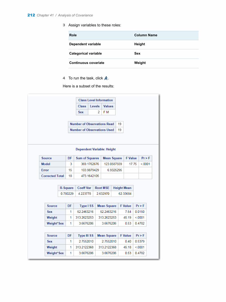
3 Assign variables to these roles:
Role Column Name
Dependent variable Height
Categorical variable Sex
Continuous covariate Weight
4 To run the task, click .
Here is a subset of the results:
212 Chapter 41 / Analysis of Covariance
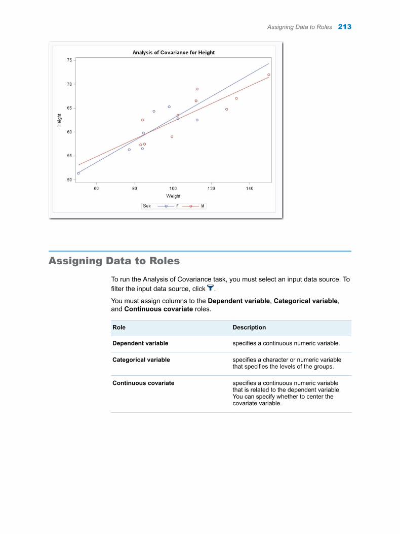
Assigning Data to Roles
To run the Analysis of Covariance task, you must select an input data source. To filter the input data source, click .
You must assign columns to the Dependent variable, Categorical variable, and Continuous covariate roles.
Role Description
Dependent variable specifies a continuous numeric variable.
Categorical variable specifies a character or numeric variable that specifies the levels of the groups.
Continuous covariate specifies a continuous numeric variable that is related to the dependent variable. You can specify whether to center the covariate variable.
Assigning Data to Roles 213
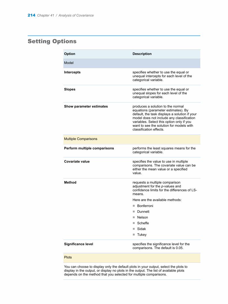
Setting Options
Option Description
Model
Intercepts specifies whether to use the equal or unequal intercepts for each level of the categorical variable.
Slopes specifies whether to use the equal or unequal slopes for each level of the categorical variable.
Show parameter estimates produces a solution to the normal equations (parameter estimates). By default, the task displays a solution if your model does not include any classification variables. Select this option only if you want to see the solution for models with classification effects.
Multiple Comparisons
Perform multiple comparisons performs the least squares means for the categorical variable.
Covariate value specifies the value to use in multiple comparisons. The covariate value can be either the mean value or a specified value.
Method requests a multiple comparison adjustment for the p-values and confidence limits for the differences of LS-means.
Here are the available methods:
n Bonferronin Dunnettn Nelsonn Scheffen Sidakn Tukey
Significance level specifies the significance level for the comparisons. The default is 0.05.
Plots
You can choose to display only the default plots in your output, select the plots to display in the output, or display no plots in the output. The list of available plots depends on the method that you selected for multiple comparisons.
214 Chapter 41 / Analysis of Covariance

Setting the Output Options
You can specify whether to create an output data set. You can also specify the values to include in the output data set. You can include predicted values, residuals, standard errors, and influence statistics.
Setting the Output Options 215

216 Chapter 41 / Analysis of Covariance
42Linear Regression
About the Linear Regression Task . . . . . . . . . . . . . . . . . . . . . . . . . . . . . . . . . . . . . . . . . 217
Example: Predicting Weight Based on a Student’s Height . . . . . . . . . . . . . . . . . . 217
Assigning Data to Roles . . . . . . . . . . . . . . . . . . . . . . . . . . . . . . . . . . . . . . . . . . . . . . . . . . . 220
Building a Model . . . . . . . . . . . . . . . . . . . . . . . . . . . . . . . . . . . . . . . . . . . . . . . . . . . . . . . . . . 222Requirements for Building a Model . . . . . . . . . . . . . . . . . . . . . . . . . . . . . . . . . . . . . . . 222Single Effects . . . . . . . . . . . . . . . . . . . . . . . . . . . . . . . . . . . . . . . . . . . . . . . . . . . . . . . . . . . 222Standard Models . . . . . . . . . . . . . . . . . . . . . . . . . . . . . . . . . . . . . . . . . . . . . . . . . . . . . . . . 223
Setting the Model Options . . . . . . . . . . . . . . . . . . . . . . . . . . . . . . . . . . . . . . . . . . . . . . . . . 224
Setting the Model Selection Options . . . . . . . . . . . . . . . . . . . . . . . . . . . . . . . . . . . . . . . 227
Creating Output Data Sets . . . . . . . . . . . . . . . . . . . . . . . . . . . . . . . . . . . . . . . . . . . . . . . . . 229
About the Linear Regression Task
The Linear regression task fits a linear model to predict a single continuous dependent variable from one or more continuous or categorical predictor variables. This task produces statistics and graphs for interpreting the results.
Note: You must license and install SAS/STAT to use this task.
Example: Predicting Weight Based on a Student’s Height
In this example, you want to use regression analysis to find out how well you can predict a child's weight if you know the child's height.
To create this example:
1 In the Tasks section, expand the Statistics folder, and then double-click Linear Regression. The user interface for the Linear Regression task opens.
2 On the Data tab, select the SASHELP.CLASS data set.
217
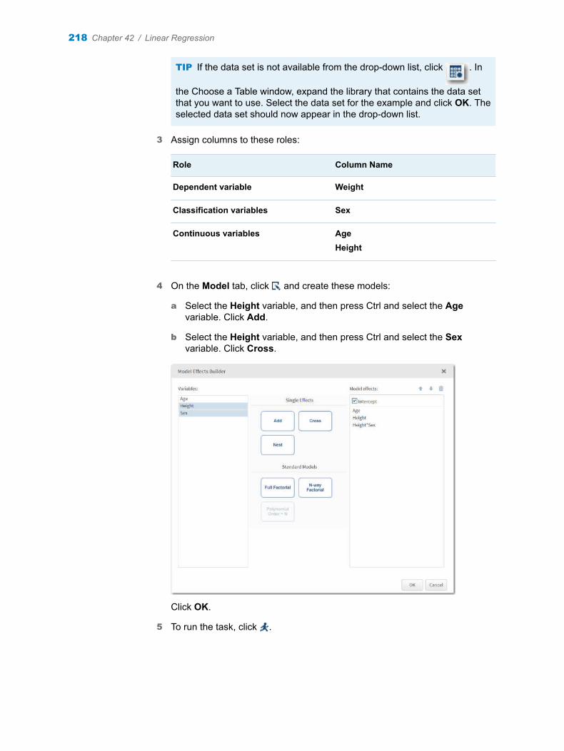
TIP If the data set is not available from the drop-down list, click . In
the Choose a Table window, expand the library that contains the data set that you want to use. Select the data set for the example and click OK. The selected data set should now appear in the drop-down list.
3 Assign columns to these roles:
Role Column Name
Dependent variable Weight
Classification variables Sex
Continuous variables AgeHeight
4 On the Model tab, click and create these models:
a Select the Height variable, and then press Ctrl and select the Age variable. Click Add.
b Select the Height variable, and then press Ctrl and select the Sex variable. Click Cross.
Click OK.
5 To run the task, click .
218 Chapter 42 / Linear Regression
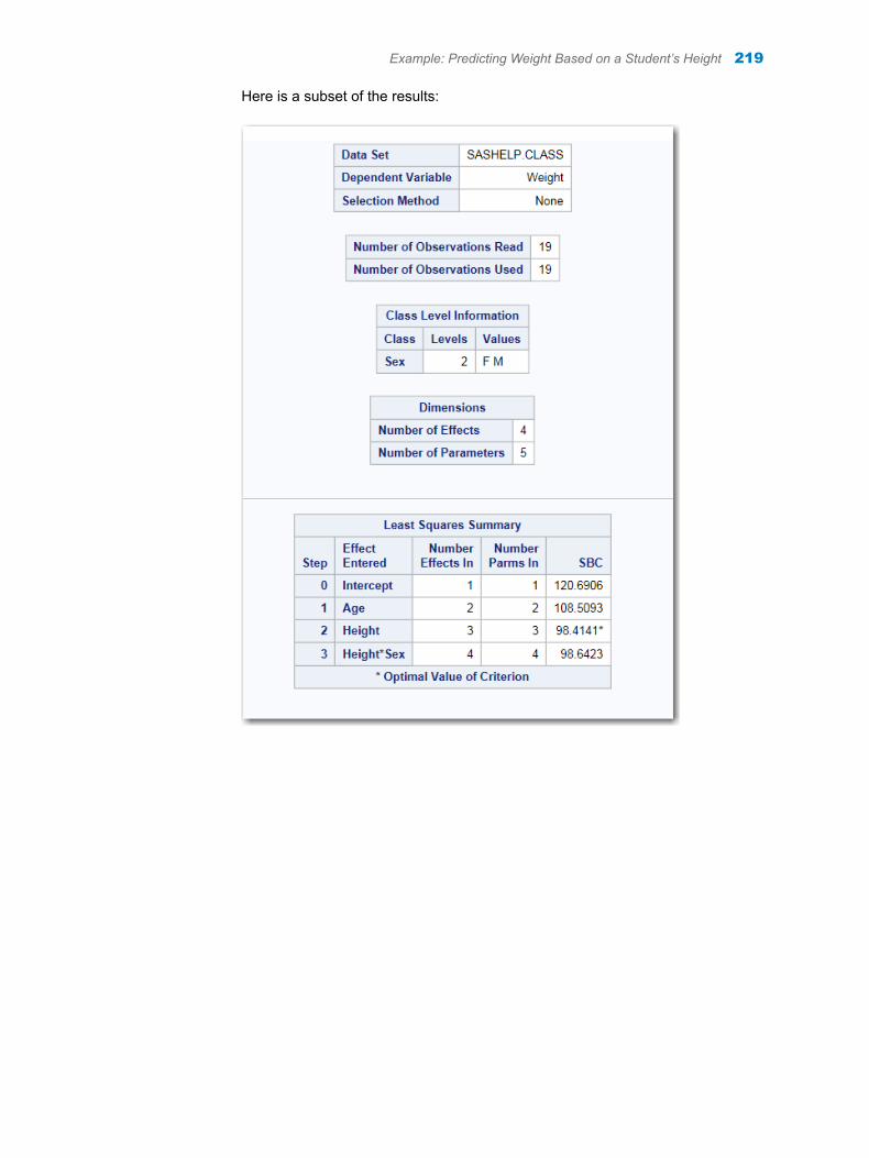
Here is a subset of the results:
Example: Predicting Weight Based on a Student’s Height 219
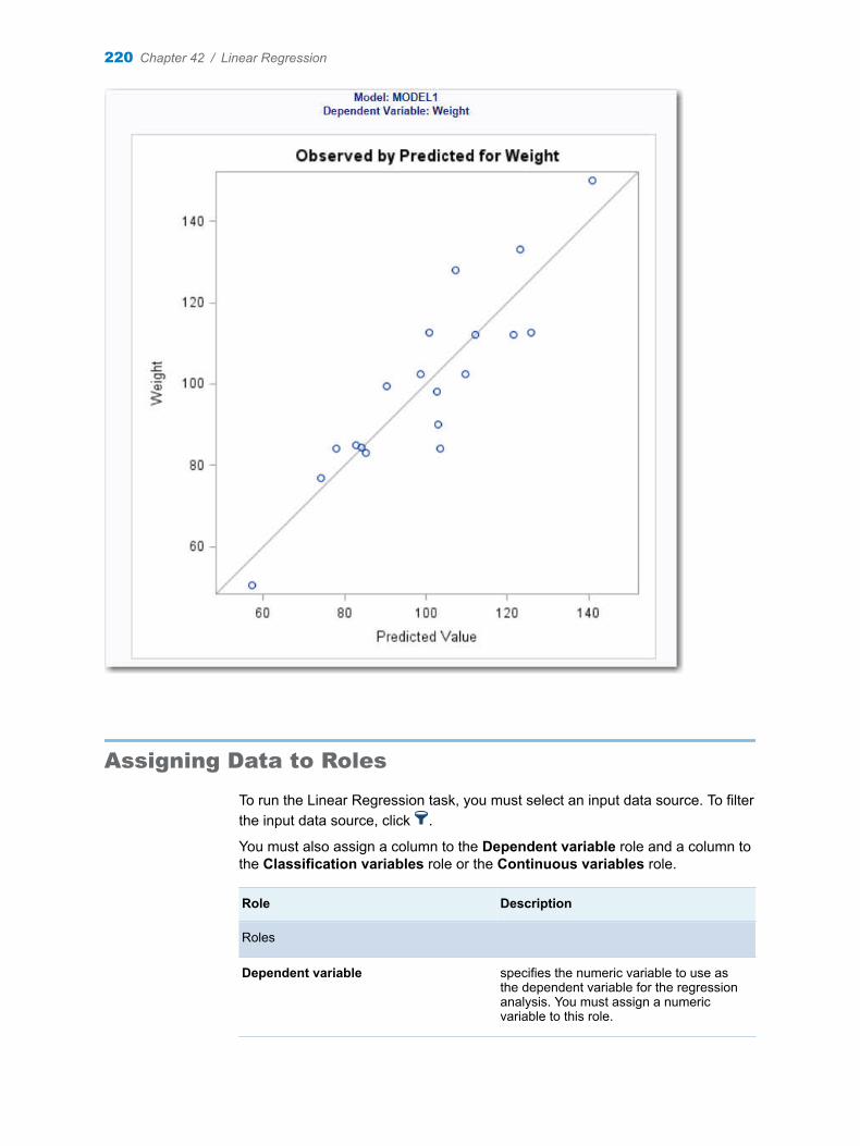
Assigning Data to Roles
To run the Linear Regression task, you must select an input data source. To filter the input data source, click .
You must also assign a column to the Dependent variable role and a column to the Classification variables role or the Continuous variables role.
Role Description
Roles
Dependent variable specifies the numeric variable to use as the dependent variable for the regression analysis. You must assign a numeric variable to this role.
220 Chapter 42 / Linear Regression
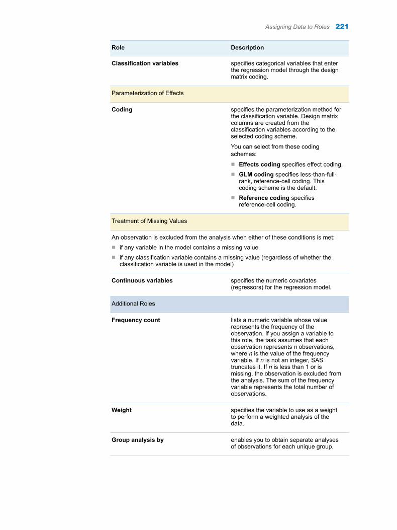
Role Description
Classification variables specifies categorical variables that enter the regression model through the design matrix coding.
Parameterization of Effects
Coding specifies the parameterization method for the classification variable. Design matrix columns are created from the classification variables according to the selected coding scheme.
You can select from these coding schemes:
n Effects coding specifies effect coding.n GLM coding specifies less-than-full-
rank, reference-cell coding. This coding scheme is the default.
n Reference coding specifies reference-cell coding.
Treatment of Missing Values
An observation is excluded from the analysis when either of these conditions is met:n if any variable in the model contains a missing valuen if any classification variable contains a missing value (regardless of whether the
classification variable is used in the model)
Continuous variables specifies the numeric covariates (regressors) for the regression model.
Additional Roles
Frequency count lists a numeric variable whose value represents the frequency of the observation. If you assign a variable to this role, the task assumes that each observation represents n observations, where n is the value of the frequency variable. If n is not an integer, SAS truncates it. If n is less than 1 or is missing, the observation is excluded from the analysis. The sum of the frequency variable represents the total number of observations.
Weight specifies the variable to use as a weight to perform a weighted analysis of the data.
Group analysis by enables you to obtain separate analyses of observations for each unique group.
Assigning Data to Roles 221
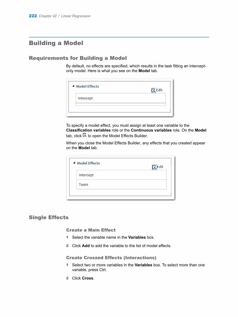
Building a Model
Requirements for Building a Model
By default, no effects are specified, which results in the task fitting an intercept-only model. Here is what you see on the Model tab.
To specify a model effect, you must assign at least one variable to the Classification variables role or the Continuous variables role. On the Model tab, click to open the Model Effects Builder.
When you close the Model Effects Builder, any effects that you created appear on the Model tab.
Single Effects
Create a Main Effect
1 Select the variable name in the Variables box.
2 Click Add to add the variable to the list of model effects.
Create Crossed Effects (Interactions)
1 Select two or more variables in the Variables box. To select more than one variable, press Ctrl.
2 Click Cross.
222 Chapter 42 / Linear Regression
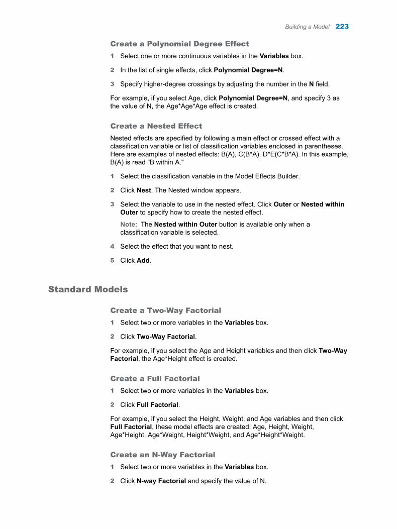
Create a Polynomial Degree Effect
1 Select one or more continuous variables in the Variables box.
2 In the list of single effects, click Polynomial Degree=N.
3 Specify higher-degree crossings by adjusting the number in the N field.
For example, if you select Age, click Polynomial Degree=N, and specify 3 as the value of N, the Age*Age*Age effect is created.
Create a Nested Effect
Nested effects are specified by following a main effect or crossed effect with a classification variable or list of classification variables enclosed in parentheses. Here are examples of nested effects: B(A), C(B*A), D*E(C*B*A). In this example, B(A) is read "B within A."
1 Select the classification variable in the Model Effects Builder.
2 Click Nest. The Nested window appears.
3 Select the variable to use in the nested effect. Click Outer or Nested within Outer to specify how to create the nested effect.
Note: The Nested within Outer button is available only when a classification variable is selected.
4 Select the effect that you want to nest.
5 Click Add.
Standard Models
Create a Two-Way Factorial
1 Select two or more variables in the Variables box.
2 Click Two-Way Factorial.
For example, if you select the Age and Height variables and then click Two-Way Factorial, the Age*Height effect is created.
Create a Full Factorial
1 Select two or more variables in the Variables box.
2 Click Full Factorial.
For example, if you select the Height, Weight, and Age variables and then click Full Factorial, these model effects are created: Age, Height, Weight, Age*Height, Age*Weight, Height*Weight, and Age*Height*Weight.
Create an N-Way Factorial
1 Select two or more variables in the Variables box.
2 Click N-way Factorial and specify the value of N.
Building a Model 223
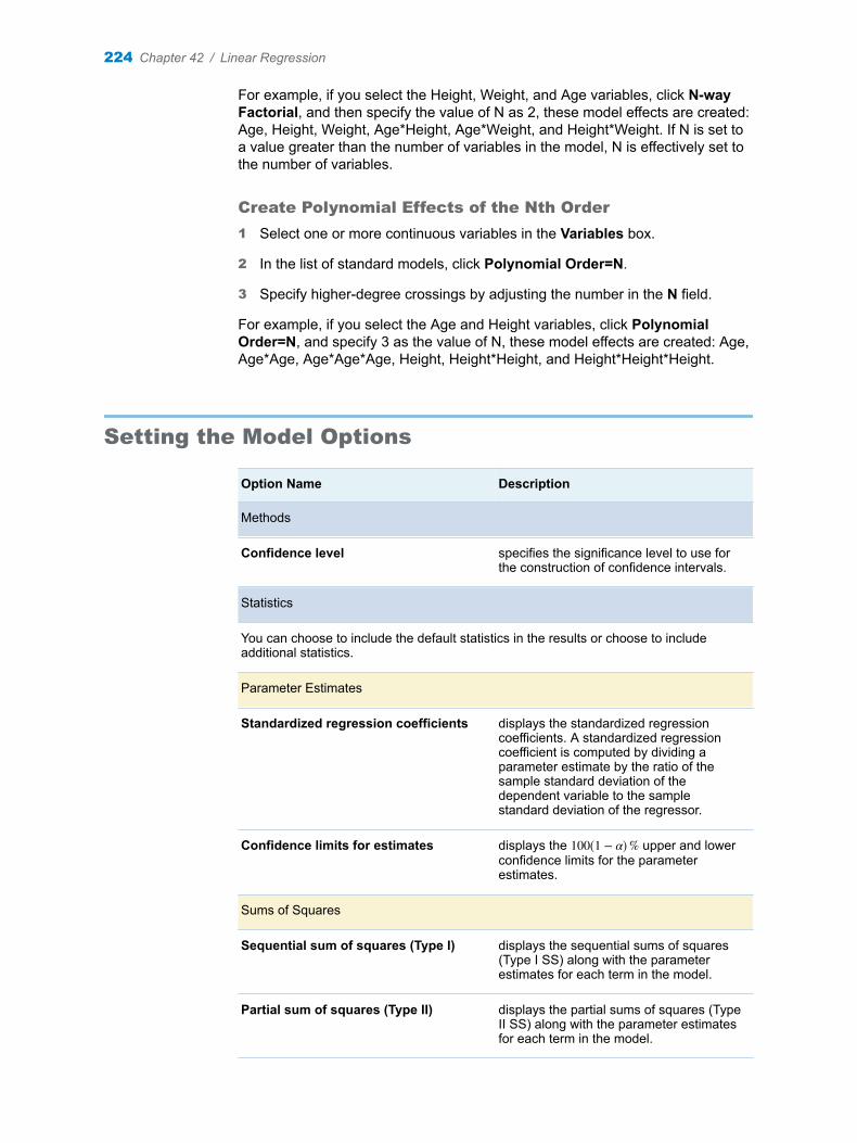
For example, if you select the Height, Weight, and Age variables, click N-way Factorial, and then specify the value of N as 2, these model effects are created: Age, Height, Weight, Age*Height, Age*Weight, and Height*Weight. If N is set to a value greater than the number of variables in the model, N is effectively set to the number of variables.
Create Polynomial Effects of the Nth Order
1 Select one or more continuous variables in the Variables box.
2 In the list of standard models, click Polynomial Order=N.
3 Specify higher-degree crossings by adjusting the number in the N field.
For example, if you select the Age and Height variables, click Polynomial Order=N, and specify 3 as the value of N, these model effects are created: Age, Age*Age, Age*Age*Age, Height, Height*Height, and Height*Height*Height.
Setting the Model Options
Option Name Description
Methods
Confidence level specifies the significance level to use for the construction of confidence intervals.
Statistics
You can choose to include the default statistics in the results or choose to include additional statistics.
Parameter Estimates
Standardized regression coefficients displays the standardized regression coefficients. A standardized regression coefficient is computed by dividing a parameter estimate by the ratio of the sample standard deviation of the dependent variable to the sample standard deviation of the regressor.
Confidence limits for estimates displays the 100 1 − α % upper and lower confidence limits for the parameter estimates.
Sums of Squares
Sequential sum of squares (Type I) displays the sequential sums of squares (Type I SS) along with the parameter estimates for each term in the model.
Partial sum of squares (Type II) displays the partial sums of squares (Type II SS) along with the parameter estimates for each term in the model.
224 Chapter 42 / Linear Regression
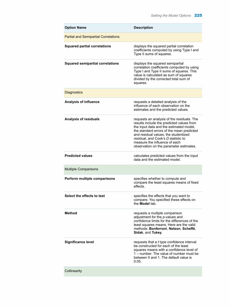
Option Name Description
Partial and Semipartial Correlations
Squared partial correlations displays the squared partial correlation coefficients computed by using Type I and Type II sums of squares.
Squared semipartial correlations displays the squared semipartial correlation coefficients computed by using Type I and Type II sums of squares. This value is calculated as sum of squares divided by the corrected total sum of squares.
Diagnostics
Analysis of influence requests a detailed analysis of the influence of each observation on the estimates and the predicted values.
Analysis of residuals requests an analysis of the residuals. The results include the predicted values from the input data and the estimated model, the standard errors of the mean predicted and residual values, the studentized residual, and Cook’s D statistic to measure the influence of each observation on the parameter estimates.
Predicted values calculates predicted values from the input data and the estimated model.
Multiple Comparisons
Perform multiple comparisons specifies whether to compute and compare the least squares means of fixed effects.
Select the effects to test specifies the effects that you want to compare. You specified these effects on the Model tab.
Method requests a multiple comparison adjustment for the p-values and confidence limits for the differences of the least squares means. Here are the valid methods: Bonferroni, Nelson, Scheffé, Sidak, and Tukey.
Significance level requests that a t type confidence interval be constructed for each of the least squares means with a confidence level of 1 – number. The value of number must be between 0 and 1. The default value is 0.05.
Collinearity
Setting the Model Options 225
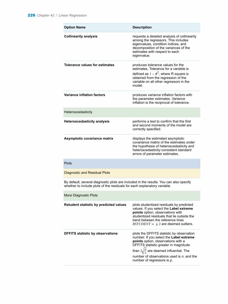
Option Name Description
Collinearity analysis requests a detailed analysis of collinearity among the regressors. This includes eigenvalues, condition indices, and decomposition of the variances of the estimates with respect to each eigenvalue.
Tolerance values for estimates produces tolerance values for the estimates. Tolerance for a variable is defined as 1 − R2, where R square is obtained from the regression of the variable on all other regressors in the model.
Variance inflation factors produces variance inflation factors with the parameter estimates. Variance inflation is the reciprocal of tolerance.
Heteroscedasticity
Heteroscedasticity analysis performs a test to confirm that the first and second moments of the model are correctly specified.
Asymptotic covariance matrix displays the estimated asymptotic covariance matrix of the estimates under the hypothesis of heteroscedasticity and heteroscedasticity-consistent standard errors of parameter estimates.
Plots
Diagnostic and Residual Plots
By default, several diagnostic plots are included in the results. You can also specify whether to include plots of the residuals for each explanatory variable.
More Diagnostic Plots
Rstudent statistic by predicted values plots studentized residuals by predicted values. If you select the Label extreme points option, observations with studentized residuals that lie outside the band between the reference lines RSTUDENT = ± 2 are deemed outliers.
DFFITS statistic by observations plots the DFFITS statistic by observation number. If you select the Label extreme points option, observations with a DFFITS statistic greater in magnitude
than 2 pn are deemed influential. The
number of observations used is n, and the number of regressors is p.
226 Chapter 42 / Linear Regression
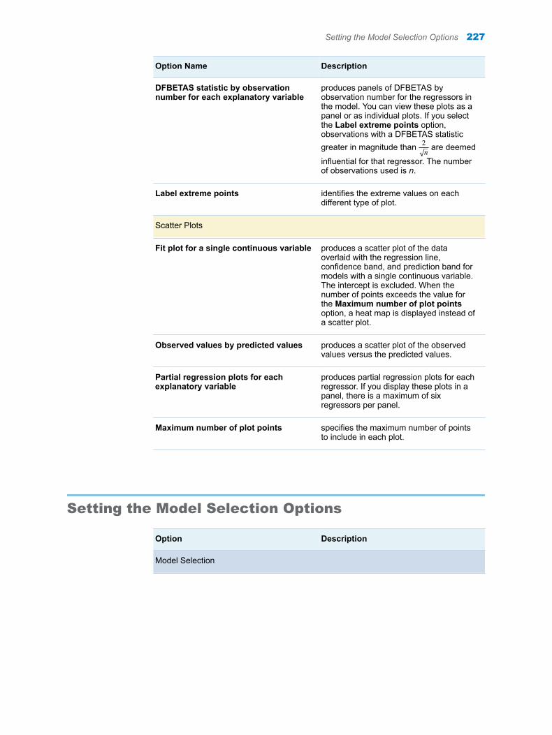
Option Name Description
DFBETAS statistic by observation number for each explanatory variable
produces panels of DFBETAS by observation number for the regressors in the model. You can view these plots as a panel or as individual plots. If you select the Label extreme points option, observations with a DFBETAS statistic greater in magnitude than 2
n are deemed
influential for that regressor. The number of observations used is n.
Label extreme points identifies the extreme values on each different type of plot.
Scatter Plots
Fit plot for a single continuous variable produces a scatter plot of the data overlaid with the regression line, confidence band, and prediction band for models with a single continuous variable. The intercept is excluded. When the number of points exceeds the value for the Maximum number of plot points option, a heat map is displayed instead of a scatter plot.
Observed values by predicted values produces a scatter plot of the observed values versus the predicted values.
Partial regression plots for each explanatory variable
produces partial regression plots for each regressor. If you display these plots in a panel, there is a maximum of six regressors per panel.
Maximum number of plot points specifies the maximum number of points to include in each plot.
Setting the Model Selection Options
Option Description
Model Selection
Setting the Model Selection Options 227
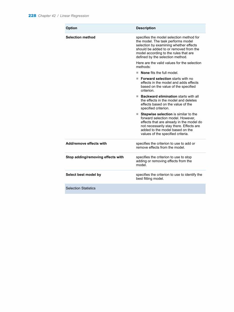
Option Description
Selection method specifies the model selection method for the model. The task performs model selection by examining whether effects should be added to or removed from the model according to the rules that are defined by the selection method.
Here are the valid values for the selection methods:n None fits the full model.n Forward selection starts with no
effects in the model and adds effects based on the value of the specified criterion.
n Backward elimination starts with all the effects in the model and deletes effects based on the value of the specified criterion.
n Stepwise selection is similar to the forward selection model. However, effects that are already in the model do not necessarily stay there. Effects are added to the model based on the values of the specified criteria.
Add/remove effects with specifies the criterion to use to add or remove effects from the model.
Stop adding/removing effects with specifies the criterion to use to stop adding or removing effects from the model.
Select best model by specifies the criterion to use to identify the best fitting model.
Selection Statistics
228 Chapter 42 / Linear Regression
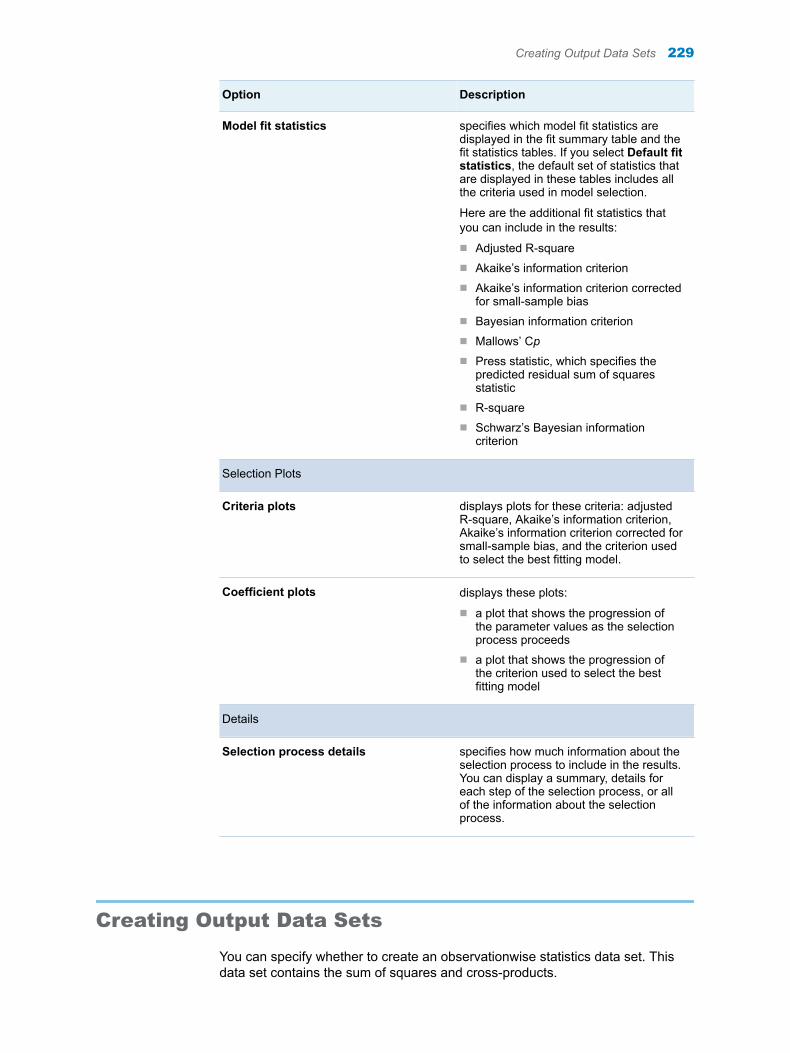
Option Description
Model fit statistics specifies which model fit statistics are displayed in the fit summary table and the fit statistics tables. If you select Default fit statistics, the default set of statistics that are displayed in these tables includes all the criteria used in model selection.
Here are the additional fit statistics that you can include in the results:
n Adjusted R-squaren Akaike’s information criterionn Akaike’s information criterion corrected
for small-sample biasn Bayesian information criterionn Mallows’ Cpn Press statistic, which specifies the
predicted residual sum of squares statistic
n R-squaren Schwarz’s Bayesian information
criterion
Selection Plots
Criteria plots displays plots for these criteria: adjusted R-square, Akaike’s information criterion, Akaike’s information criterion corrected for small-sample bias, and the criterion used to select the best fitting model.
Coefficient plots displays these plots:
n a plot that shows the progression of the parameter values as the selection process proceeds
n a plot that shows the progression of the criterion used to select the best fitting model
Details
Selection process details specifies how much information about the selection process to include in the results. You can display a summary, details for each step of the selection process, or all of the information about the selection process.
Creating Output Data Sets
You can specify whether to create an observationwise statistics data set. This data set contains the sum of squares and cross-products.
Creating Output Data Sets 229
You can also choose to include these statistics in the output data set:
n predicted values
n press statistic, which is the ith residual divided by 1 − h , where h is the leverage, and where the model has been refit without the ith observation
n residual
n studentized residuals, which are the residuals divided by their standard errors
n studentized residual with current observation removed
n Cook’s D influence
n the standard influence of observation on covariance of betas
n the standard influence of an observation on predicted value (called DFFITS)
n leverage
230 Chapter 42 / Linear Regression
43Binary Logistic Regression
About the Binary Logistic Regression Task . . . . . . . . . . . . . . . . . . . . . . . . . . . . . . . . 231
Example: Classifying Email as Junk . . . . . . . . . . . . . . . . . . . . . . . . . . . . . . . . . . . . . . . 231
Assigning Data to Roles . . . . . . . . . . . . . . . . . . . . . . . . . . . . . . . . . . . . . . . . . . . . . . . . . . . 233
Building a Model . . . . . . . . . . . . . . . . . . . . . . . . . . . . . . . . . . . . . . . . . . . . . . . . . . . . . . . . . . 235Create a Main Effect . . . . . . . . . . . . . . . . . . . . . . . . . . . . . . . . . . . . . . . . . . . . . . . . . . . . . 235Create Crossed Effects (Interactions) . . . . . . . . . . . . . . . . . . . . . . . . . . . . . . . . . . . . . 235Create a Nested Effect . . . . . . . . . . . . . . . . . . . . . . . . . . . . . . . . . . . . . . . . . . . . . . . . . . . 236Create a Full Factorial Model . . . . . . . . . . . . . . . . . . . . . . . . . . . . . . . . . . . . . . . . . . . . . 236Create an N-Way Factorial . . . . . . . . . . . . . . . . . . . . . . . . . . . . . . . . . . . . . . . . . . . . . . . 236Create Polynomial Effects of the Nth Order . . . . . . . . . . . . . . . . . . . . . . . . . . . . . . . . 236Setting the Model Options . . . . . . . . . . . . . . . . . . . . . . . . . . . . . . . . . . . . . . . . . . . . . . . 237
Specifying the Model Selection Options . . . . . . . . . . . . . . . . . . . . . . . . . . . . . . . . . . . 237
Setting Options . . . . . . . . . . . . . . . . . . . . . . . . . . . . . . . . . . . . . . . . . . . . . . . . . . . . . . . . . . . . 239
Creating Output Data Sets . . . . . . . . . . . . . . . . . . . . . . . . . . . . . . . . . . . . . . . . . . . . . . . . . 242
About the Binary Logistic Regression Task
The Binary Logistic Regression task is used to fit a logistic regression model to investigate the relationship between discrete responses with binary levels and a set of explanatory variables.
Note: You must license and install SAS/STAT to use this task.
Example: Classifying Email as Junk
To create this example:
1 In the Tasks section, expand the Statistics folder, and then double-click Binary Logistic Regression. The user interface for the Binary Logistic Regression task opens.
2 On the Data tab, select the SASHELP.JUNKMAIL data set.
3 Assign columns to these roles and specify these options:
231
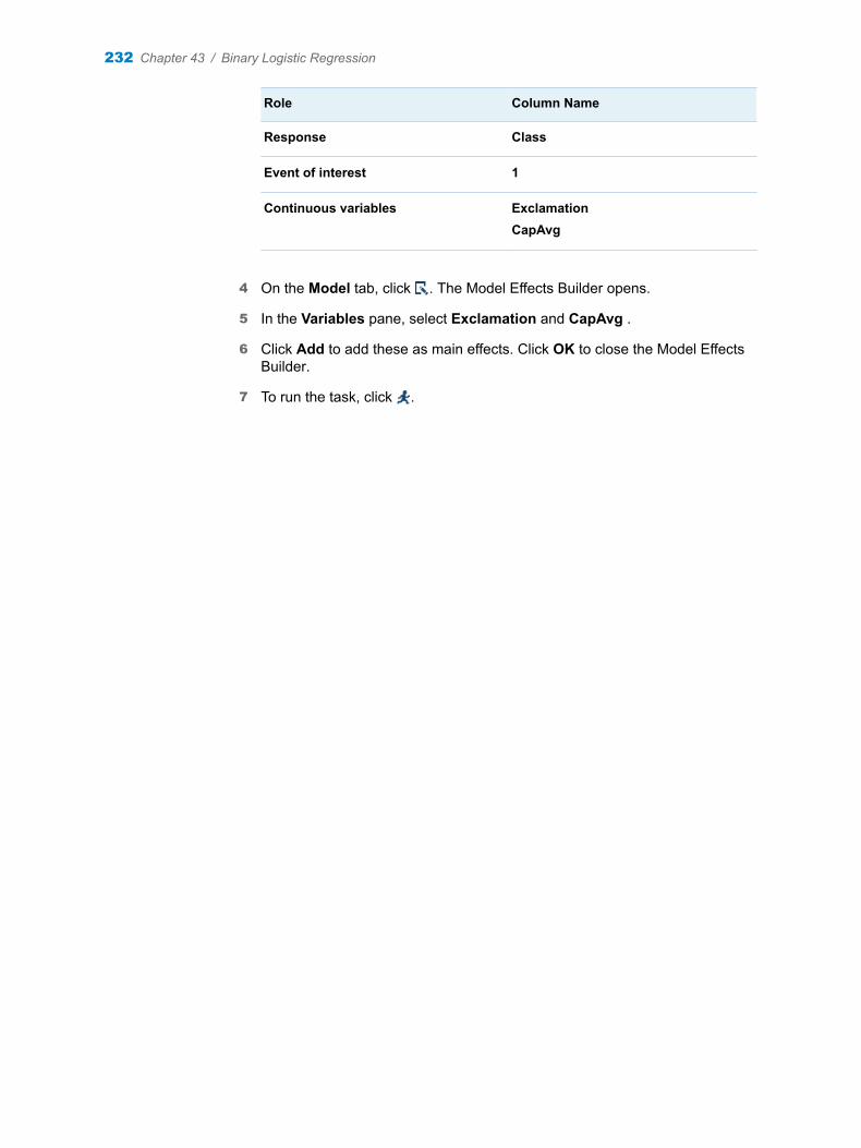
Role Column Name
Response Class
Event of interest 1
Continuous variables ExclamationCapAvg
4 On the Model tab, click . The Model Effects Builder opens.
5 In the Variables pane, select Exclamation and CapAvg .
6 Click Add to add these as main effects. Click OK to close the Model Effects Builder.
7 To run the task, click .
232 Chapter 43 / Binary Logistic Regression
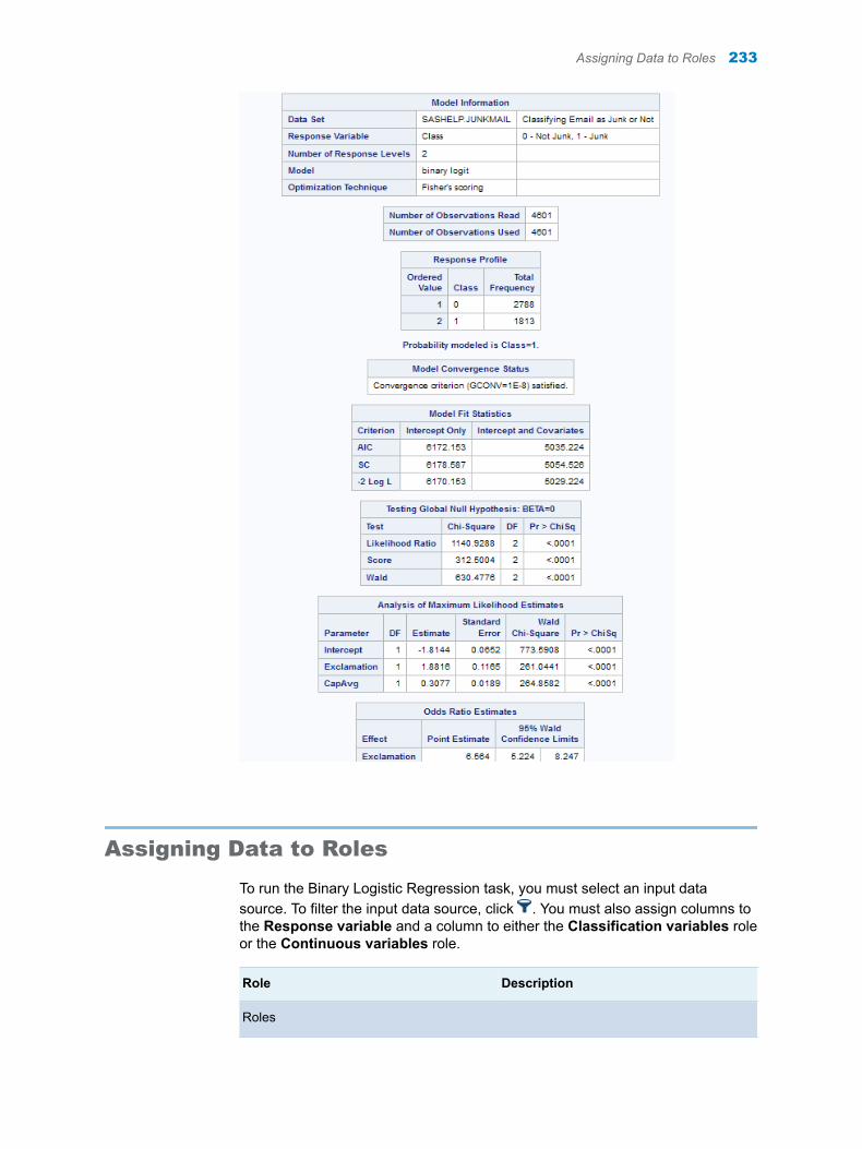
Assigning Data to Roles
To run the Binary Logistic Regression task, you must select an input data source. To filter the input data source, click . You must also assign columns to the Response variable and a column to either the Classification variables role or the Continuous variables role.
Role Description
Roles
Assigning Data to Roles 233
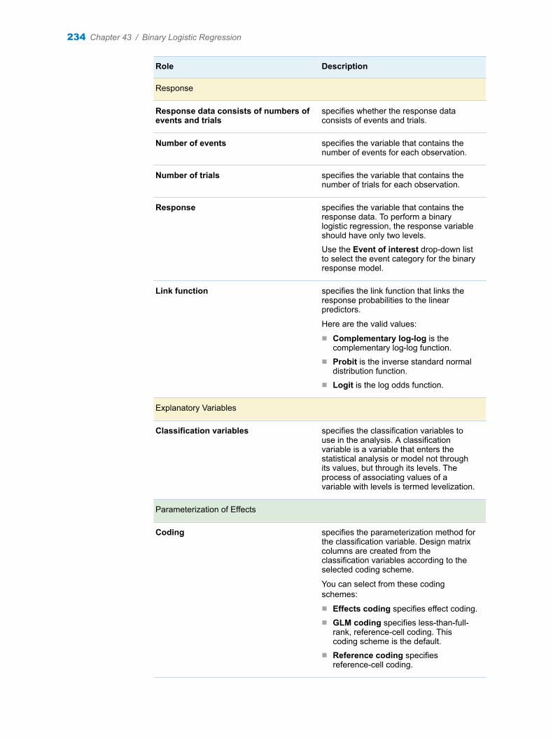
Role Description
Response
Response data consists of numbers of events and trials
specifies whether the response data consists of events and trials.
Number of events specifies the variable that contains the number of events for each observation.
Number of trials specifies the variable that contains the number of trials for each observation.
Response specifies the variable that contains the response data. To perform a binary logistic regression, the response variable should have only two levels.
Use the Event of interest drop-down list to select the event category for the binary response model.
Link function specifies the link function that links the response probabilities to the linear predictors.
Here are the valid values:
n Complementary log-log is the complementary log-log function.
n Probit is the inverse standard normal distribution function.
n Logit is the log odds function.
Explanatory Variables
Classification variables specifies the classification variables to use in the analysis. A classification variable is a variable that enters the statistical analysis or model not through its values, but through its levels. The process of associating values of a variable with levels is termed levelization.
Parameterization of Effects
Coding specifies the parameterization method for the classification variable. Design matrix columns are created from the classification variables according to the selected coding scheme.
You can select from these coding schemes:
n Effects coding specifies effect coding.n GLM coding specifies less-than-full-
rank, reference-cell coding. This coding scheme is the default.
n Reference coding specifies reference-cell coding.
234 Chapter 43 / Binary Logistic Regression

Role Description
Treatment of Missing Values
An observation is excluded from the analysis when either of these conditions is met:n if any variable in the model contains a missing valuen if any classification variable contains a missing value (regardless of whether the
classification variable is used in the model)
Continuous variables specifies the continuous variables to use as the explanatory variables in the analysis.
Additional Roles
Stratify by specifies the variables that define the strata or matched sets to use in stratified logistic regression of binary response data.
Frequency count specifies the variables that contain the frequency of occurrence for each observation. The task treats each observation as if it appears n times, where n is the value of the variable for that observation.
Weight variable specifies the how much to weight each observation in the input data set.
Group analysis by creates separate analyses based on the number of BY variables.
Building a Model
Create a Main Effect
1 Select the variable name in the Variables box.
2 Click Add to add the variable to the list of model effects.
Create Crossed Effects (Interactions)
1 Select two or more variables in the Variables box. To select more than one variable, press Ctrl.
2 Click Cross.
Building a Model 235
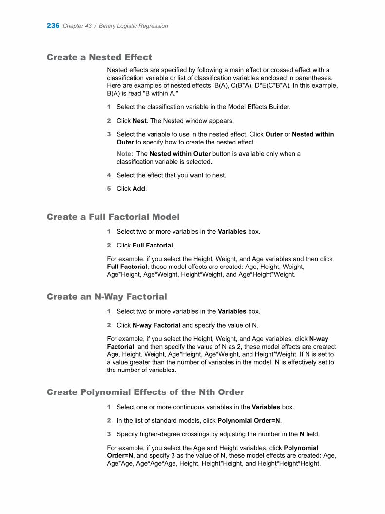
Create a Nested Effect
Nested effects are specified by following a main effect or crossed effect with a classification variable or list of classification variables enclosed in parentheses. Here are examples of nested effects: B(A), C(B*A), D*E(C*B*A). In this example, B(A) is read "B within A."
1 Select the classification variable in the Model Effects Builder.
2 Click Nest. The Nested window appears.
3 Select the variable to use in the nested effect. Click Outer or Nested within Outer to specify how to create the nested effect.
Note: The Nested within Outer button is available only when a classification variable is selected.
4 Select the effect that you want to nest.
5 Click Add.
Create a Full Factorial Model
1 Select two or more variables in the Variables box.
2 Click Full Factorial.
For example, if you select the Height, Weight, and Age variables and then click Full Factorial, these model effects are created: Age, Height, Weight, Age*Height, Age*Weight, Height*Weight, and Age*Height*Weight.
Create an N-Way Factorial
1 Select two or more variables in the Variables box.
2 Click N-way Factorial and specify the value of N.
For example, if you select the Height, Weight, and Age variables, click N-way Factorial, and then specify the value of N as 2, these model effects are created: Age, Height, Weight, Age*Height, Age*Weight, and Height*Weight. If N is set to a value greater than the number of variables in the model, N is effectively set to the number of variables.
Create Polynomial Effects of the Nth Order
1 Select one or more continuous variables in the Variables box.
2 In the list of standard models, click Polynomial Order=N.
3 Specify higher-degree crossings by adjusting the number in the N field.
For example, if you select the Age and Height variables, click Polynomial Order=N, and specify 3 as the value of N, these model effects are created: Age, Age*Age, Age*Age*Age, Height, Height*Height, and Height*Height*Height.
236 Chapter 43 / Binary Logistic Regression
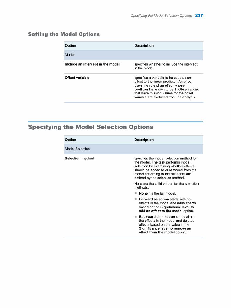
Setting the Model Options
Option Description
Model
Include an intercept in the model specifies whether to include the intercept in the model.
Offset variable specifies a variable to be used as an offset to the linear predictor. An offset plays the role of an effect whose coefficient is known to be 1. Observations that have missing values for the offset variable are excluded from the analysis.
Specifying the Model Selection Options
Option Description
Model Selection
Selection method specifies the model selection method for the model. The task performs model selection by examining whether effects should be added to or removed from the model according to the rules that are defined by the selection method.
Here are the valid values for the selection methods:n None fits the full model.n Forward selection starts with no
effects in the model and adds effects based on the Significance level to add an effect to the model option.
n Backward elimination starts with all the effects in the model and deletes effects based on the value in the Significance level to remove an effect from the model option.
Specifying the Model Selection Options 237
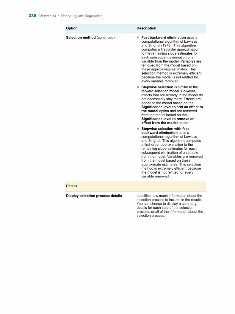
Option Description
Selection method (continued) n Fast backward elimination uses a computational algorithm of Lawless and Singhal (1978). This algorithm computes a first-order approximation to the remaining slope estimates for each subsequent elimination of a variable from the model. Variables are removed from the model based on these approximate estimates. This selection method is extremely efficient because the model is not refitted for every variable removed.
n Stepwise selection is similar to the forward selection model. However, effects that are already in the model do not necessarily stay there. Effects are added to the model based on the Significance level to add an effect to the model option and are removed from the model based on the Significance level to remove an effect from the model option.
n Stepwise selection with fast backward elimination uses a computational algorithm of Lawless and Singhal. This algorithm computes a first-order approximation to the remaining slope estimates for each subsequent elimination of a variable from the model. Variables are removed from the model based on these approximate estimates. This selection method is extremely efficient because the model is not refitted for every variable removed.
Details
Display selection process details specifies how much information about the selection process to include in the results. You can choose to display a summary, details for each step of the selection process, or all of the information about the selection process.
238 Chapter 43 / Binary Logistic Regression
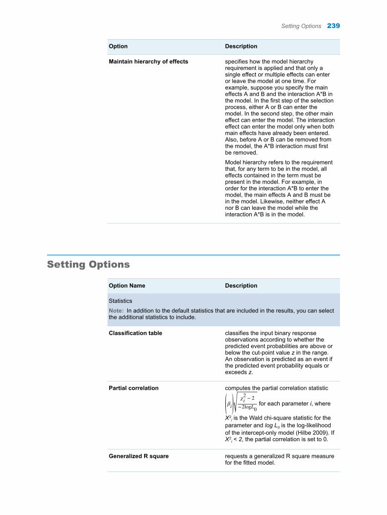
Option Description
Maintain hierarchy of effects specifies how the model hierarchy requirement is applied and that only a single effect or multiple effects can enter or leave the model at one time. For example, suppose you specify the main effects A and B and the interaction A*B in the model. In the first step of the selection process, either A or B can enter the model. In the second step, the other main effect can enter the model. The interaction effect can enter the model only when both main effects have already been entered. Also, before A or B can be removed from the model, the A*B interaction must first be removed.
Model hierarchy refers to the requirement that, for any term to be in the model, all effects contained in the term must be present in the model. For example, in order for the interaction A*B to enter the model, the main effects A and B must be in the model. Likewise, neither effect A nor B can leave the model while the interaction A*B is in the model.
Setting Options
Option Name Description
Statistics
Note: In addition to the default statistics that are included in the results, you can select the additional statistics to include.
Classification table classifies the input binary response observations according to whether the predicted event probabilities are above or below the cut-point value z in the range. An observation is predicted as an event if the predicted event probability equals or exceeds z.
Partial correlation computes the partial correlation statistic
βiχi2 − 2
−2logL0 for each parameter i, where
X2i is the Wald chi-square statistic for the
parameter and log L0 is the log-likelihood of the intercept-only model (Hilbe 2009). If X2
i < 2, the partial correlation is set to 0.
Generalized R square requests a generalized R square measure for the fitted model.
Setting Options 239
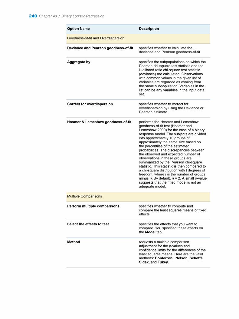
Option Name Description
Goodness-of-fit and Overdispersion
Deviance and Pearson goodness-of-fit specifies whether to calculate the deviance and Pearson goodness-of-fit.
Aggregate by specifies the subpopulations on which the Pearson chi-square test statistic and the likelihood ratio chi-square test statistic (deviance) are calculated. Observations with common values in the given list of variables are regarded as coming from the same subpopulation. Variables in the list can be any variables in the input data set.
Correct for overdispersion specifies whether to correct for overdispersion by using the Deviance or Pearson estimate.
Hosmer & Lemeshow goodness-of-fit performs the Hosmer and Lemeshow goodness-of-fit test (Hosmer and Lemeshow 2000) for the case of a binary response model. The subjects are divided into approximately 10 groups of approximately the same size based on the percentiles of the estimated probabilities. The discrepancies between the observed and expected number of observations in these groups are summarized by the Pearson chi-square statistic. This statistic is then compared to a chi-square distribution with t degrees of freedom, where t is the number of groups minus n. By default, n = 2. A small p-value suggests that the fitted model is not an adequate model.
Multiple Comparisons
Perform multiple comparisons specifies whether to compute and compare the least squares means of fixed effects.
Select the effects to test specifies the effects that you want to compare. You specified these effects on the Model tab.
Method requests a multiple comparison adjustment for the p-values and confidence limits for the differences of the least squares means. Here are the valid methods: Bonferroni, Nelson, Scheffé, Sidak, and Tukey.
240 Chapter 43 / Binary Logistic Regression
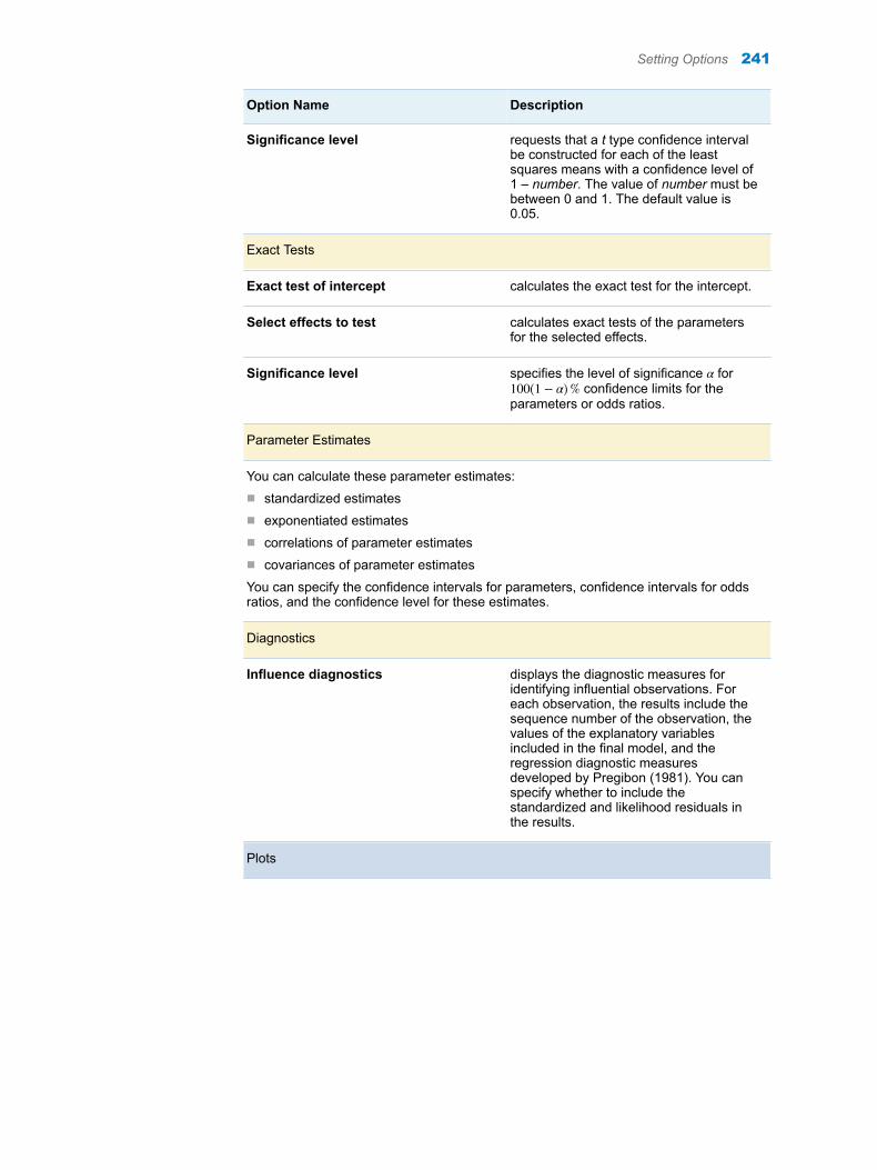
Option Name Description
Significance level requests that a t type confidence interval be constructed for each of the least squares means with a confidence level of 1 – number. The value of number must be between 0 and 1. The default value is 0.05.
Exact Tests
Exact test of intercept calculates the exact test for the intercept.
Select effects to test calculates exact tests of the parameters for the selected effects.
Significance level specifies the level of significance α for 100 1 − α % confidence limits for the parameters or odds ratios.
Parameter Estimates
You can calculate these parameter estimates:n standardized estimatesn exponentiated estimatesn correlations of parameter estimatesn covariances of parameter estimates
You can specify the confidence intervals for parameters, confidence intervals for odds ratios, and the confidence level for these estimates.
Diagnostics
Influence diagnostics displays the diagnostic measures for identifying influential observations. For each observation, the results include the sequence number of the observation, the values of the explanatory variables included in the final model, and the regression diagnostic measures developed by Pregibon (1981). You can specify whether to include the standardized and likelihood residuals in the results.
Plots
Setting Options 241
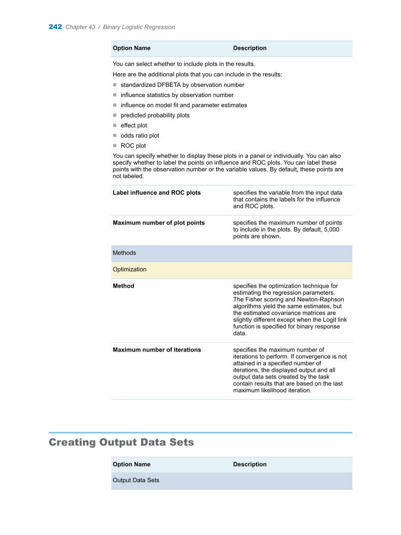
Option Name Description
You can select whether to include plots in the results.
Here are the additional plots that you can include in the results:
n standardized DFBETA by observation numbern influence statistics by observation numbern influence on model fit and parameter estimatesn predicted probability plotsn effect plotn odds ratio plotn ROC plot
You can specify whether to display these plots in a panel or individually. You can also specify whether to label the points on influence and ROC plots. You can label these points with the observation number or the variable values. By default, these points are not labeled.
Label influence and ROC plots specifies the variable from the input data that contains the labels for the influence and ROC plots.
Maximum number of plot points specifies the maximum number of points to include in the plots. By default, 5,000 points are shown.
Methods
Optimization
Method specifies the optimization technique for estimating the regression parameters. The Fisher scoring and Newton-Raphson algorithms yield the same estimates, but the estimated covariance matrices are slightly different except when the Logit link function is specified for binary response data.
Maximum number of iterations specifies the maximum number of iterations to perform. If convergence is not attained in a specified number of iterations, the displayed output and all output data sets created by the task contain results that are based on the last maximum likelihood iteration.
Creating Output Data Sets
Option Name Description
Output Data Sets
242 Chapter 43 / Binary Logistic Regression
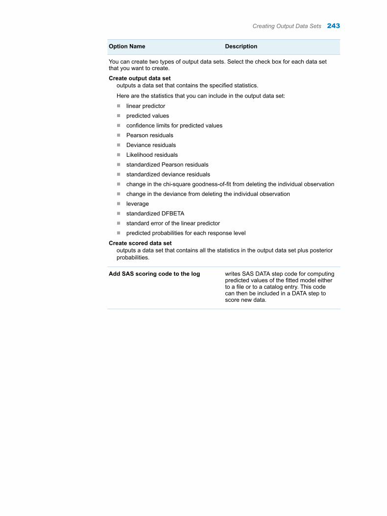
Option Name Description
You can create two types of output data sets. Select the check box for each data set that you want to create.
Create output data setoutputs a data set that contains the specified statistics.
Here are the statistics that you can include in the output data set:
n linear predictorn predicted valuesn confidence limits for predicted valuesn Pearson residualsn Deviance residualsn Likelihood residualsn standardized Pearson residualsn standardized deviance residualsn change in the chi-square goodness-of-fit from deleting the individual observationn change in the deviance from deleting the individual observationn leveragen standardized DFBETAn standard error of the linear predictorn predicted probabilities for each response level
Create scored data setoutputs a data set that contains all the statistics in the output data set plus posterior probabilities.
Add SAS scoring code to the log writes SAS DATA step code for computing predicted values of the fitted model either to a file or to a catalog entry. This code can then be included in a DATA step to score new data.
Creating Output Data Sets 243

244 Chapter 43 / Binary Logistic Regression
44Predictive Regression Models
About the Predictive Regression Models Task . . . . . . . . . . . . . . . . . . . . . . . . . . . . . 245
Example: Predicting a Baseball Player’s Salary . . . . . . . . . . . . . . . . . . . . . . . . . . . . 246
Partitioning Data . . . . . . . . . . . . . . . . . . . . . . . . . . . . . . . . . . . . . . . . . . . . . . . . . . . . . . . . . . 248
Assigning Data to Roles . . . . . . . . . . . . . . . . . . . . . . . . . . . . . . . . . . . . . . . . . . . . . . . . . . . 249
Building a Model . . . . . . . . . . . . . . . . . . . . . . . . . . . . . . . . . . . . . . . . . . . . . . . . . . . . . . . . . . 250Requirements for Building a Model . . . . . . . . . . . . . . . . . . . . . . . . . . . . . . . . . . . . . . . 250Single Effects . . . . . . . . . . . . . . . . . . . . . . . . . . . . . . . . . . . . . . . . . . . . . . . . . . . . . . . . . . . 251Standard Models . . . . . . . . . . . . . . . . . . . . . . . . . . . . . . . . . . . . . . . . . . . . . . . . . . . . . . . . 252
Selecting a Model . . . . . . . . . . . . . . . . . . . . . . . . . . . . . . . . . . . . . . . . . . . . . . . . . . . . . . . . . 253
Setting the Options for the Final Model . . . . . . . . . . . . . . . . . . . . . . . . . . . . . . . . . . . . 257
Setting the Scoring Options . . . . . . . . . . . . . . . . . . . . . . . . . . . . . . . . . . . . . . . . . . . . . . . 258
About the Predictive Regression Models Task
The task is predictive in that it selects the most influential effects based on observed data. This task enables you to logically partition your data into disjoint subsets for model training, validation, and testing. The Predictive Regression Models task focuses on the standard independently and identically distributed general linear model for univariate responses and offers great flexibility and insight into the model selection algorithm. This task can also create a scored data set. The results for this task make it easy to explore the selected model in more detail with other tasks, such as the Linear Regression task.
Note: You must license and install SAS/STAT to use this task.
245
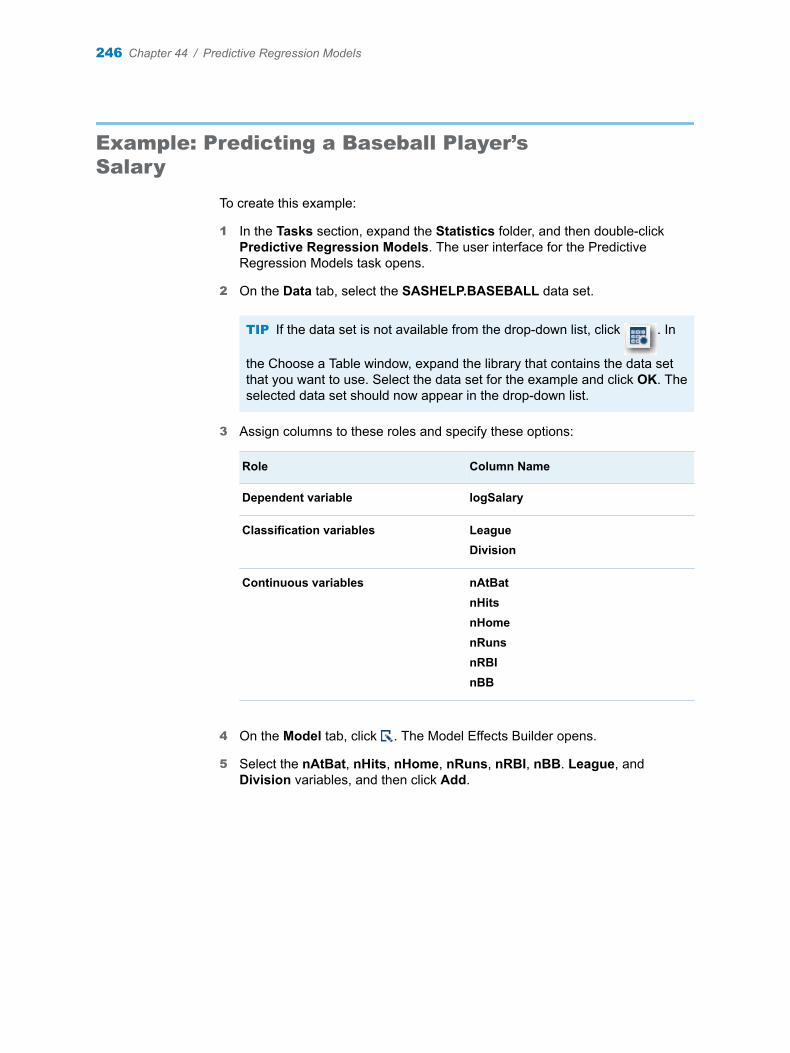
Example: Predicting a Baseball Player’s Salary
To create this example:
1 In the Tasks section, expand the Statistics folder, and then double-click Predictive Regression Models. The user interface for the Predictive Regression Models task opens.
2 On the Data tab, select the SASHELP.BASEBALL data set.
TIP If the data set is not available from the drop-down list, click . In
the Choose a Table window, expand the library that contains the data set that you want to use. Select the data set for the example and click OK. The selected data set should now appear in the drop-down list.
3 Assign columns to these roles and specify these options:
Role Column Name
Dependent variable logSalary
Classification variables LeagueDivision
Continuous variables nAtBatnHitsnHomenRunsnRBInBB
4 On the Model tab, click . The Model Effects Builder opens.
5 Select the nAtBat, nHits, nHome, nRuns, nRBI, nBB. League, and Division variables, and then click Add.
246 Chapter 44 / Predictive Regression Models
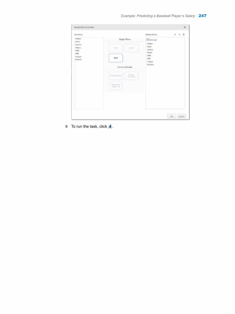
6 To run the task, click .
Example: Predicting a Baseball Player’s Salary 247
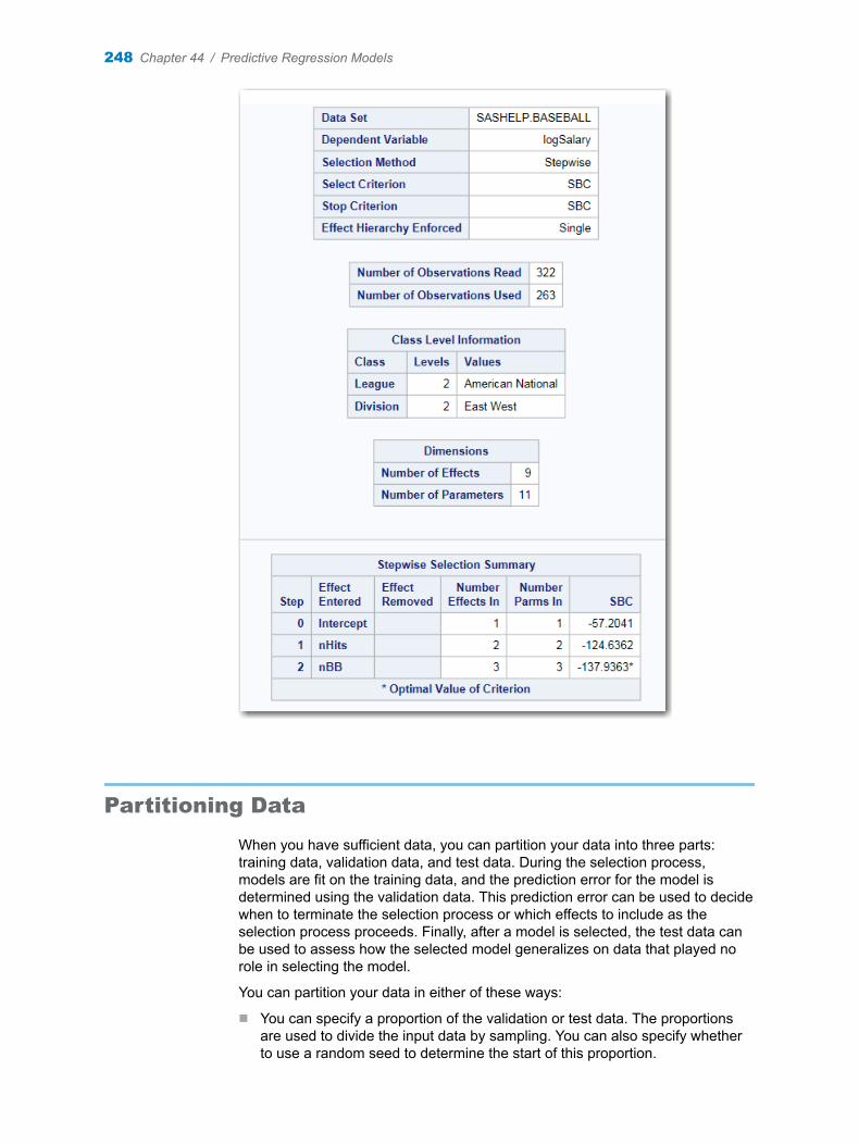
Partitioning Data
When you have sufficient data, you can partition your data into three parts: training data, validation data, and test data. During the selection process, models are fit on the training data, and the prediction error for the model is determined using the validation data. This prediction error can be used to decide when to terminate the selection process or which effects to include as the selection process proceeds. Finally, after a model is selected, the test data can be used to assess how the selected model generalizes on data that played no role in selecting the model.
You can partition your data in either of these ways:
n You can specify a proportion of the validation or test data. The proportions are used to divide the input data by sampling. You can also specify whether to use a random seed to determine the start of this proportion.
248 Chapter 44 / Predictive Regression Models
n If the input data set contains a variable whose values indicate whether an observation is a validation or test case, you can specify the variable to use when partitioning the data. When you specify the variable, you also select the appropriate values for validation or test cases. The input data set is divided into partitions by using these values.
Assigning Data to Roles
To run the Predictive Regression Models task, you must select an input data source. To filter the input data source, click .
You also must assign a column to the Dependent variable role and a column to the Classification variables role or the Continuous variables role.
Role Description
Roles
Dependent variable specifies the numeric variable to use as the dependent variable for the regression analysis.
Classification variables specifies the variables to use to group (classify) data in the analysis. A classification variable is a variable that enters the statistical analysis or model through its levels, not through its values. The process of associating values of a variable with levels is termed levelization.
Parameterization of Effects
Coding specifies the parameterization method for the classification variable. Design matrix columns are created from the classification variables according to the selected coding scheme.
You can select from these coding schemes:
n Effects coding specifies effect coding.n GLM coding specifies less-than-full-
rank, reference-cell coding. This coding scheme is the default.
n Reference coding specifies reference-cell coding.
Treatment of Missing Values
An observation is excluded from the analysis if any variable in the model contains a missing value. In addition, an observation is excluded if any classification variable specified earlier in this table contains a missing value, regardless if it is used in the model.
Assigning Data to Roles 249
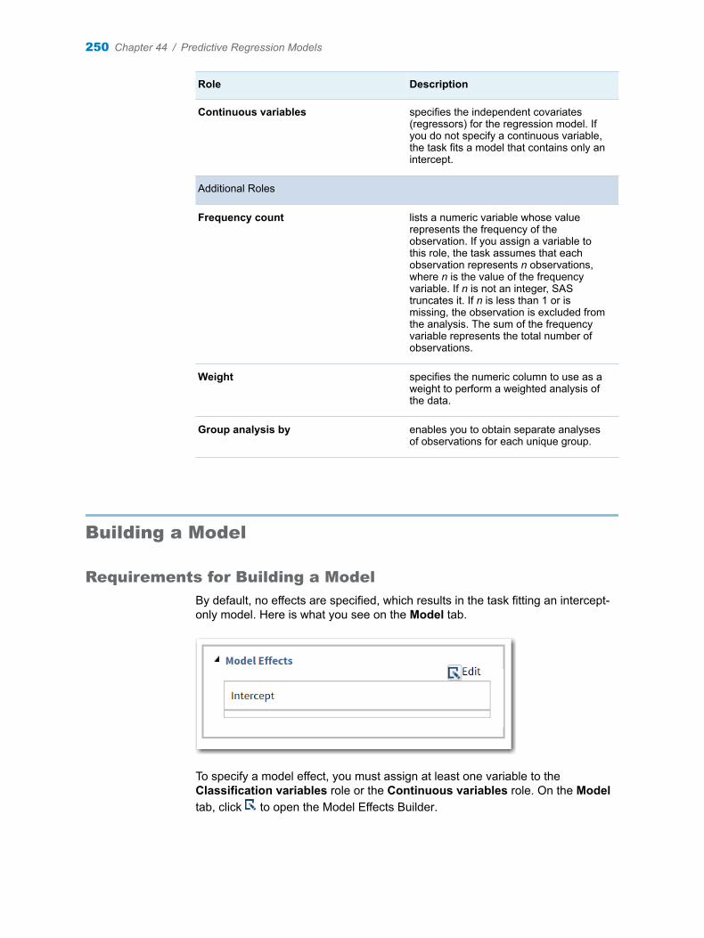
Role Description
Continuous variables specifies the independent covariates (regressors) for the regression model. If you do not specify a continuous variable, the task fits a model that contains only an intercept.
Additional Roles
Frequency count lists a numeric variable whose value represents the frequency of the observation. If you assign a variable to this role, the task assumes that each observation represents n observations, where n is the value of the frequency variable. If n is not an integer, SAS truncates it. If n is less than 1 or is missing, the observation is excluded from the analysis. The sum of the frequency variable represents the total number of observations.
Weight specifies the numeric column to use as a weight to perform a weighted analysis of the data.
Group analysis by enables you to obtain separate analyses of observations for each unique group.
Building a Model
Requirements for Building a Model
By default, no effects are specified, which results in the task fitting an intercept-only model. Here is what you see on the Model tab.
To specify a model effect, you must assign at least one variable to the Classification variables role or the Continuous variables role. On the Model tab, click to open the Model Effects Builder.
250 Chapter 44 / Predictive Regression Models
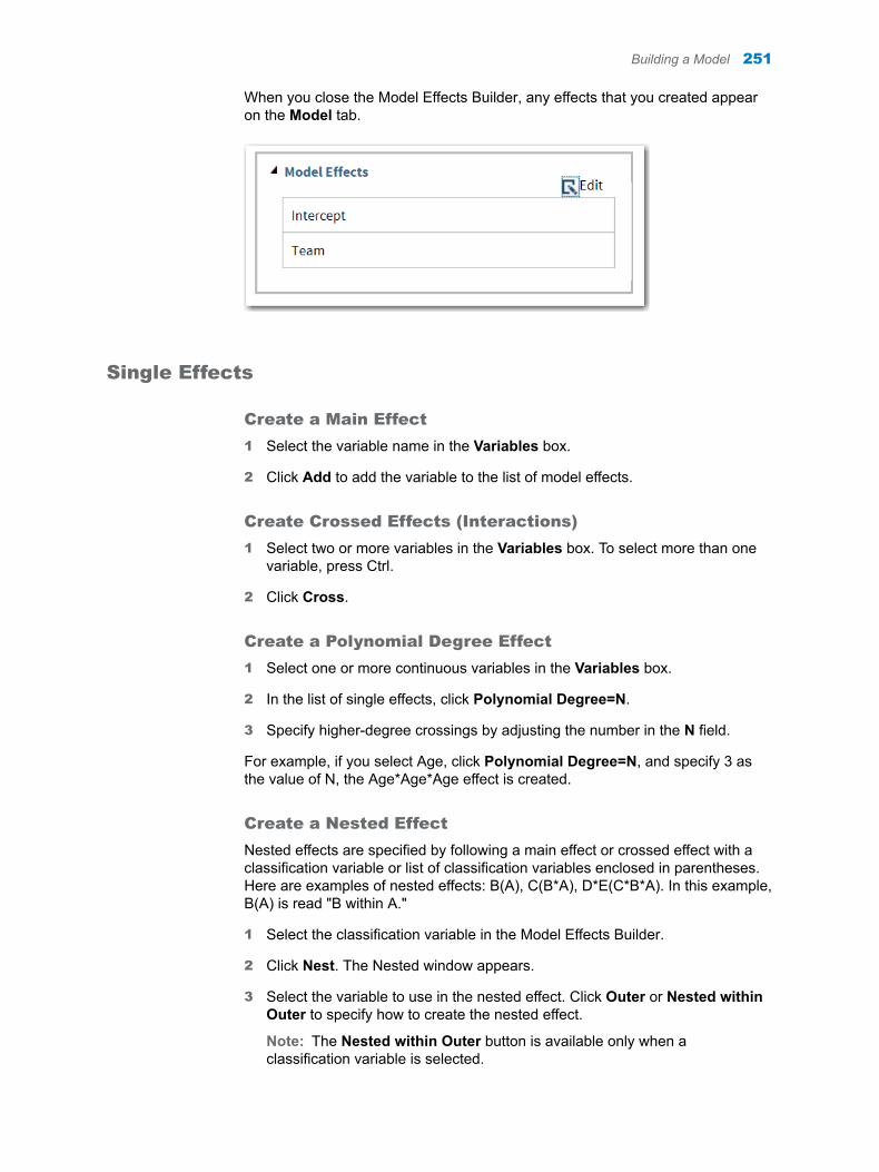
When you close the Model Effects Builder, any effects that you created appear on the Model tab.
Single Effects
Create a Main Effect
1 Select the variable name in the Variables box.
2 Click Add to add the variable to the list of model effects.
Create Crossed Effects (Interactions)
1 Select two or more variables in the Variables box. To select more than one variable, press Ctrl.
2 Click Cross.
Create a Polynomial Degree Effect
1 Select one or more continuous variables in the Variables box.
2 In the list of single effects, click Polynomial Degree=N.
3 Specify higher-degree crossings by adjusting the number in the N field.
For example, if you select Age, click Polynomial Degree=N, and specify 3 as the value of N, the Age*Age*Age effect is created.
Create a Nested Effect
Nested effects are specified by following a main effect or crossed effect with a classification variable or list of classification variables enclosed in parentheses. Here are examples of nested effects: B(A), C(B*A), D*E(C*B*A). In this example, B(A) is read "B within A."
1 Select the classification variable in the Model Effects Builder.
2 Click Nest. The Nested window appears.
3 Select the variable to use in the nested effect. Click Outer or Nested within Outer to specify how to create the nested effect.
Note: The Nested within Outer button is available only when a classification variable is selected.
Building a Model 251
4 Select the effect that you want to nest.
5 Click Add.
Standard Models
Create a Two-Way Factorial
1 Select two or more variables in the Variables box.
2 Click Two-Way Factorial.
For example, if you select the Age and Height variables and then click Two-Way Factorial, the Age*Height effect is created.
Create a Full Factorial
1 Select two or more variables in the Variables box.
2 Click Full Factorial.
For example, if you select the Height, Weight, and Age variables and then click Full Factorial, these model effects are created: Age, Height, Weight, Age*Height, Age*Weight, Height*Weight, and Age*Height*Weight.
Create an N-Way Factorial
1 Select two or more variables in the Variables box.
2 Click N-way Factorial and specify the value of N.
For example, if you select the Height, Weight, and Age variables, click N-way Factorial, and then specify the value of N as 2, these model effects are created: Age, Height, Weight, Age*Height, Age*Weight, and Height*Weight. If N is set to a value greater than the number of variables in the model, N is effectively set to the number of variables.
Create Polynomial Effects of the Nth Order
1 Select one or more continuous variables in the Variables box.
2 In the list of standard models, click Polynomial Order=N.
3 Specify higher-degree crossings by adjusting the number in the N field.
For example, if you select the Age and Height variables, click Polynomial Order=N, and specify 3 as the value of N, these model effects are created: Age, Age*Age, Age*Age*Age, Height, Height*Height, and Height*Height*Height.
252 Chapter 44 / Predictive Regression Models
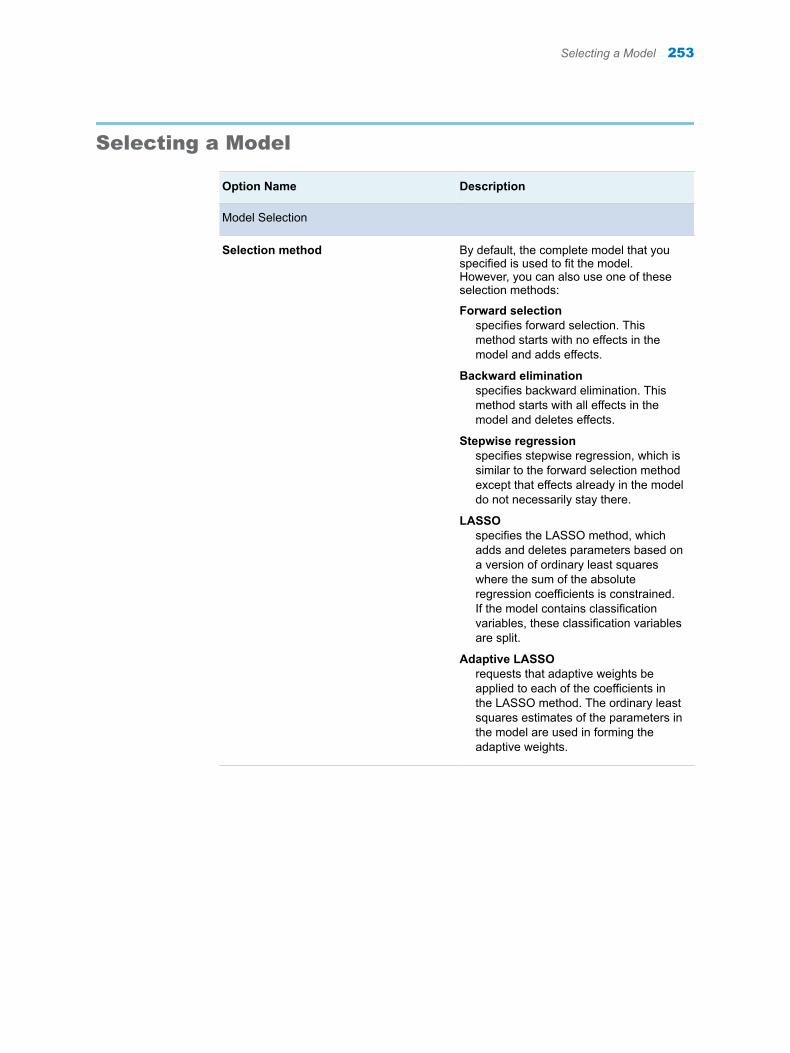
Selecting a Model
Option Name Description
Model Selection
Selection method By default, the complete model that you specified is used to fit the model. However, you can also use one of these selection methods:
Forward selectionspecifies forward selection. This method starts with no effects in the model and adds effects.
Backward eliminationspecifies backward elimination. This method starts with all effects in the model and deletes effects.
Stepwise regressionspecifies stepwise regression, which is similar to the forward selection method except that effects already in the model do not necessarily stay there.
LASSOspecifies the LASSO method, which adds and deletes parameters based on a version of ordinary least squares where the sum of the absolute regression coefficients is constrained. If the model contains classification variables, these classification variables are split.
Adaptive LASSOrequests that adaptive weights be applied to each of the coefficients in the LASSO method. The ordinary least squares estimates of the parameters in the model are used in forming the adaptive weights.
Selecting a Model 253
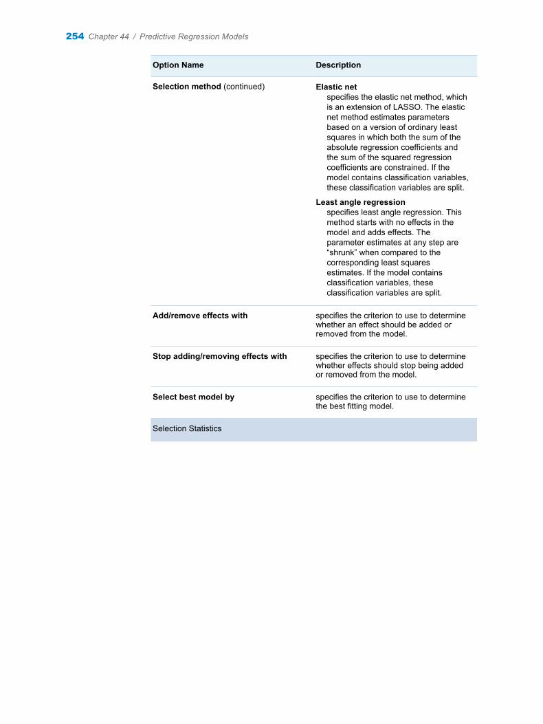
Option Name Description
Selection method (continued) Elastic netspecifies the elastic net method, which is an extension of LASSO. The elastic net method estimates parameters based on a version of ordinary least squares in which both the sum of the absolute regression coefficients and the sum of the squared regression coefficients are constrained. If the model contains classification variables, these classification variables are split.
Least angle regressionspecifies least angle regression. This method starts with no effects in the model and adds effects. The parameter estimates at any step are “shrunk” when compared to the corresponding least squares estimates. If the model contains classification variables, these classification variables are split.
Add/remove effects with specifies the criterion to use to determine whether an effect should be added or removed from the model.
Stop adding/removing effects with specifies the criterion to use to determine whether effects should stop being added or removed from the model.
Select best model by specifies the criterion to use to determine the best fitting model.
Selection Statistics
254 Chapter 44 / Predictive Regression Models
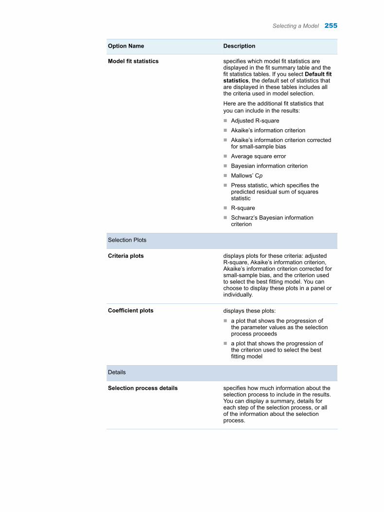
Option Name Description
Model fit statistics specifies which model fit statistics are displayed in the fit summary table and the fit statistics tables. If you select Default fit statistics, the default set of statistics that are displayed in these tables includes all the criteria used in model selection.
Here are the additional fit statistics that you can include in the results:
n Adjusted R-squaren Akaike’s information criterionn Akaike’s information criterion corrected
for small-sample biasn Average square errorn Bayesian information criterionn Mallows’ Cpn Press statistic, which specifies the
predicted residual sum of squares statistic
n R-squaren Schwarz’s Bayesian information
criterion
Selection Plots
Criteria plots displays plots for these criteria: adjusted R-square, Akaike’s information criterion, Akaike’s information criterion corrected for small-sample bias, and the criterion used to select the best fitting model. You can choose to display these plots in a panel or individually.
Coefficient plots displays these plots:
n a plot that shows the progression of the parameter values as the selection process proceeds
n a plot that shows the progression of the criterion used to select the best fitting model
Details
Selection process details specifies how much information about the selection process to include in the results. You can display a summary, details for each step of the selection process, or all of the information about the selection process.
Selecting a Model 255
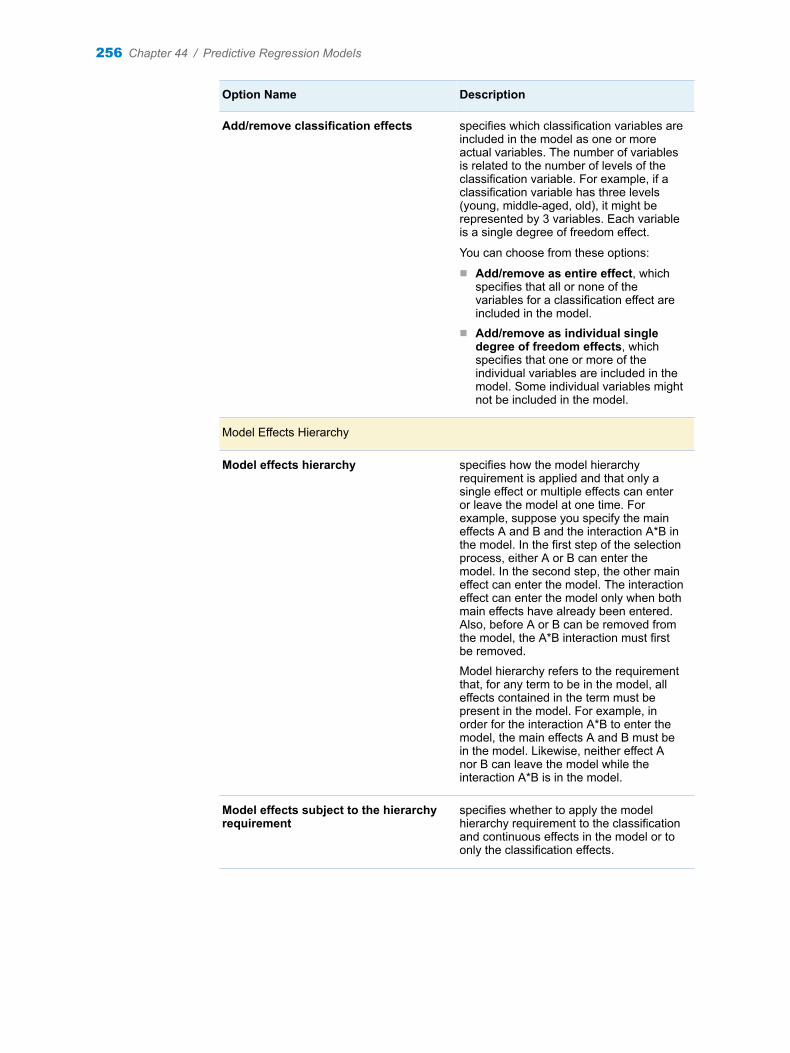
Option Name Description
Add/remove classification effects specifies which classification variables are included in the model as one or more actual variables. The number of variables is related to the number of levels of the classification variable. For example, if a classification variable has three levels (young, middle-aged, old), it might be represented by 3 variables. Each variable is a single degree of freedom effect.
You can choose from these options:
n Add/remove as entire effect, which specifies that all or none of the variables for a classification effect are included in the model.
n Add/remove as individual single degree of freedom effects, which specifies that one or more of the individual variables are included in the model. Some individual variables might not be included in the model.
Model Effects Hierarchy
Model effects hierarchy specifies how the model hierarchy requirement is applied and that only a single effect or multiple effects can enter or leave the model at one time. For example, suppose you specify the main effects A and B and the interaction A*B in the model. In the first step of the selection process, either A or B can enter the model. In the second step, the other main effect can enter the model. The interaction effect can enter the model only when both main effects have already been entered. Also, before A or B can be removed from the model, the A*B interaction must first be removed.
Model hierarchy refers to the requirement that, for any term to be in the model, all effects contained in the term must be present in the model. For example, in order for the interaction A*B to enter the model, the main effects A and B must be in the model. Likewise, neither effect A nor B can leave the model while the interaction A*B is in the model.
Model effects subject to the hierarchy requirement
specifies whether to apply the model hierarchy requirement to the classification and continuous effects in the model or to only the classification effects.
256 Chapter 44 / Predictive Regression Models
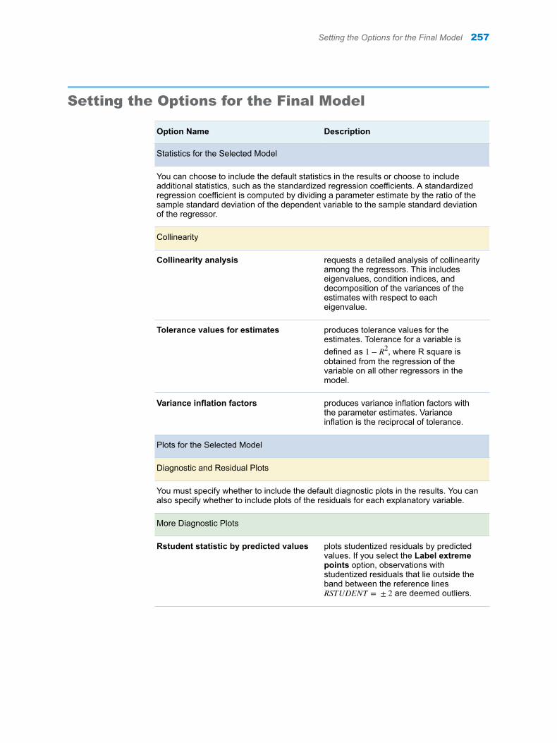
Setting the Options for the Final Model
Option Name Description
Statistics for the Selected Model
You can choose to include the default statistics in the results or choose to include additional statistics, such as the standardized regression coefficients. A standardized regression coefficient is computed by dividing a parameter estimate by the ratio of the sample standard deviation of the dependent variable to the sample standard deviation of the regressor.
Collinearity
Collinearity analysis requests a detailed analysis of collinearity among the regressors. This includes eigenvalues, condition indices, and decomposition of the variances of the estimates with respect to each eigenvalue.
Tolerance values for estimates produces tolerance values for the estimates. Tolerance for a variable is defined as 1 − R2, where R square is obtained from the regression of the variable on all other regressors in the model.
Variance inflation factors produces variance inflation factors with the parameter estimates. Variance inflation is the reciprocal of tolerance.
Plots for the Selected Model
Diagnostic and Residual Plots
You must specify whether to include the default diagnostic plots in the results. You can also specify whether to include plots of the residuals for each explanatory variable.
More Diagnostic Plots
Rstudent statistic by predicted values plots studentized residuals by predicted values. If you select the Label extreme points option, observations with studentized residuals that lie outside the band between the reference lines RSTUDENT = ± 2 are deemed outliers.
Setting the Options for the Final Model 257
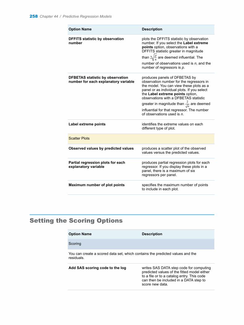
Option Name Description
DFFITS statistic by observation number
plots the DFFITS statistic by observation number. If you select the Label extreme points option, observations with a DFFITS statistic greater in magnitude
than 2 pn are deemed influential. The
number of observations used is n, and the number of regressors is p.
DFBETAS statistic by observation number for each explanatory variable
produces panels of DFBETAS by observation number for the regressors in the model. You can view these plots as a panel or as individual plots. If you select the Label extreme points option, observations with a DFBETAS statistic greater in magnitude than 2
n are deemed
influential for that regressor. The number of observations used is n.
Label extreme points identifies the extreme values on each different type of plot.
Scatter Plots
Observed values by predicted values produces a scatter plot of the observed values versus the predicted values.
Partial regression plots for each explanatory variable
produces partial regression plots for each regressor. If you display these plots in a panel, there is a maximum of six regressors per panel.
Maximum number of plot points specifies the maximum number of points to include in each plot.
Setting the Scoring Options
Option Name Description
Scoring
You can create a scored data set, which contains the predicted values and the residuals.
Add SAS scoring code to the log writes SAS DATA step code for computing predicted values of the fitted model either to a file or to a catalog entry. This code can then be included in a DATA step to score new data.
258 Chapter 44 / Predictive Regression Models

45Generalized Linear Models
About the Generalized Linear Models Task . . . . . . . . . . . . . . . . . . . . . . . . . . . . . . . . 259
Example: Analyzing the Sashelp.Baseball Data Set . . . . . . . . . . . . . . . . . . . . . . . . 260
Assigning Data to Roles . . . . . . . . . . . . . . . . . . . . . . . . . . . . . . . . . . . . . . . . . . . . . . . . . . . 261
Building a Model . . . . . . . . . . . . . . . . . . . . . . . . . . . . . . . . . . . . . . . . . . . . . . . . . . . . . . . . . . 264Understanding Effects for Generalized Linear Models . . . . . . . . . . . . . . . . . . . . . . 264Requirements for Building a Model . . . . . . . . . . . . . . . . . . . . . . . . . . . . . . . . . . . . . . . 265Single Effects . . . . . . . . . . . . . . . . . . . . . . . . . . . . . . . . . . . . . . . . . . . . . . . . . . . . . . . . . . . 266Standard Models . . . . . . . . . . . . . . . . . . . . . . . . . . . . . . . . . . . . . . . . . . . . . . . . . . . . . . . . 267
Setting Options . . . . . . . . . . . . . . . . . . . . . . . . . . . . . . . . . . . . . . . . . . . . . . . . . . . . . . . . . . . . 267
Setting the Output Options . . . . . . . . . . . . . . . . . . . . . . . . . . . . . . . . . . . . . . . . . . . . . . . . 269
About the Generalized Linear Models Task
Generalized linear models are an extension of traditional linear models. In a generalized linear model, the mean of a population depends on a linear predictor through a nonlinear link function. The response probability distribution can be any member of the exponential family of distributions. Examples of generalized linear models include classical linear models with normal errors, logistic and probit models for binary data, and log-linear models for multinomial data. Other statistical models can be formulated as generalized linear models by the selection of an appropriate link function and response probability distribution.
The Generalized Linear Models task provides model fitting and model building for generalized linear models. It fits models for standard distributions such as Normal, Poisson, and Tweedie in the exponential family. This task also fits multinomial models for ordinal and nominal responses. The task provides forward, backward, and stepwise selection methods.
Note: You must license and install SAS/STAT to use this task.
259
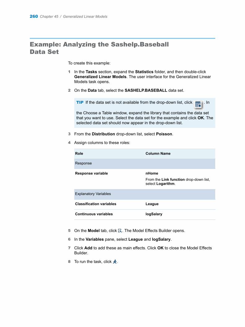
Example: Analyzing the Sashelp.Baseball Data Set
To create this example:
1 In the Tasks section, expand the Statistics folder, and then double-click Generalized Linear Models. The user interface for the Generalized Linear Models task opens.
2 On the Data tab, select the SASHELP.BASEBALL data set.
TIP If the data set is not available from the drop-down list, click . In
the Choose a Table window, expand the library that contains the data set that you want to use. Select the data set for the example and click OK. The selected data set should now appear in the drop-down list.
3 From the Distribution drop-down list, select Poisson.
4 Assign columns to these roles:
Role Column Name
Response
Response variable nHomeFrom the Link function drop-down list, select Logarithm.
Explanatory Variables
Classification variables League
Continuous variables logSalary
5 On the Model tab, click . The Model Effects Builder opens.
6 In the Variables pane, select League and logSalary.
7 Click Add to add these as main effects. Click OK to close the Model Effects Builder.
8 To run the task, click .
260 Chapter 45 / Generalized Linear Models
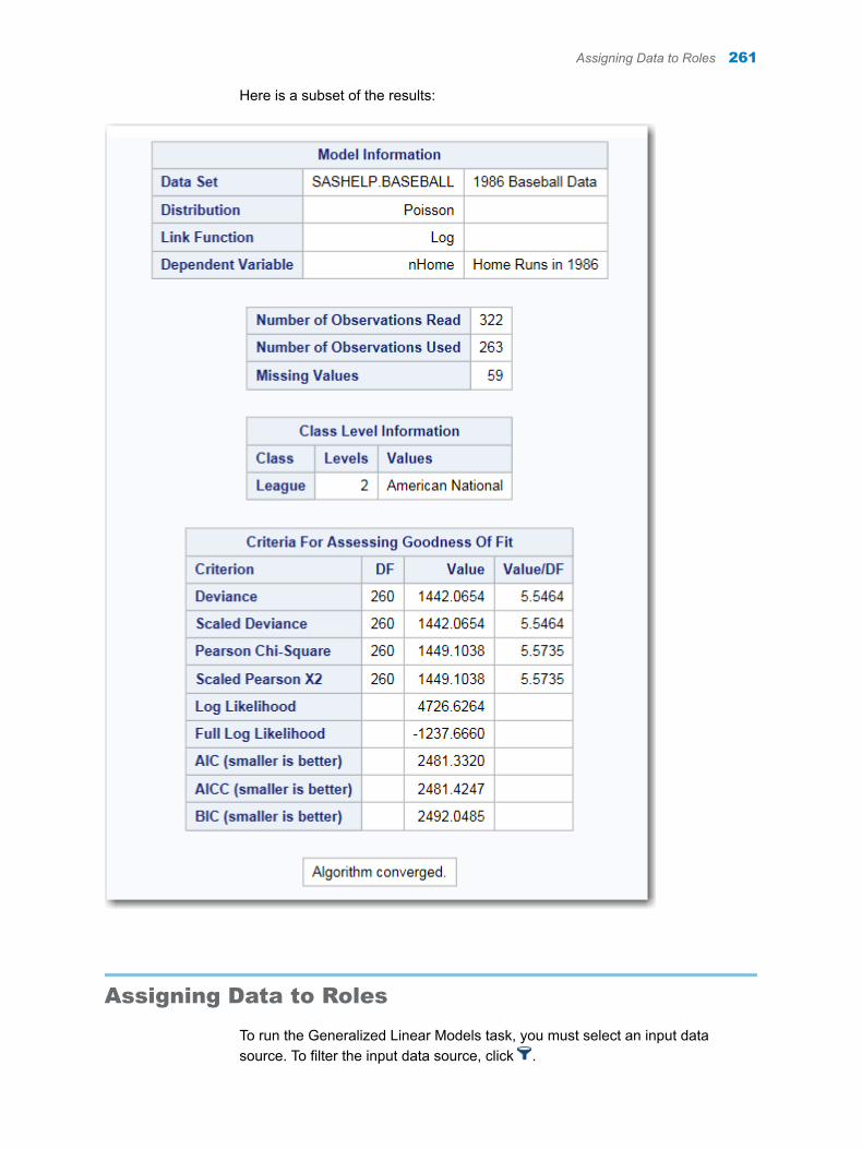
Here is a subset of the results:
Assigning Data to Roles
To run the Generalized Linear Models task, you must select an input data source. To filter the input data source, click .
Assigning Data to Roles 261
You must also assign a column to the Response variable role for all distribution types except binomial. If you select a binomial distribution, you must assign either a single response variable or a pair of variables to the Number of events and Number of trials roles.
Option Name Description
Roles
Response
Distribution specifies the distribution for your model. You can choose from these distributions:n Binomial n Gamman Inverse Gaussiann Multinomial n Negative binomialn Normaln Poissonn Tweedie. If you select a Tweedie
distribution, you can specify the Tweedie power parameter. This value must be greater than 1.1 and less than or equal to 3.0.
n Zero-inflated negative binomialn Zero-inflated Poisson
Options for Binomial Distribution
Response data consists of numbers of events and trials
specifies that a pair of variables consists of response data for events and trials.
Number of events specifies the column that contains the number of events.
Number of trials specifies the column that contains the number of trials.
Response specifies the single variable that contains response values.
Use the Event of interest option to select a value of the response variable that represents the event that you want to model.
Note: The Response role and the Event of interest option are available only if you do not select the Response data consists of numbers of events and trials check box.
Options for All Distribution Types
262 Chapter 45 / Generalized Linear Models
Option Name Description
Response specifies the variable that contains the response data. For most distribution types, you specify a single numeric variable.
Link function specifies the link function for your model. The functions that are available depend on the selected distribution.
Explanatory Variables
Classification variables specifies the variables to use to group (classify) data in the analysis. Classification variables can be either character or numeric. A classification variable is a variable that enters the statistical analysis or model through its levels, not through its values. The process of associating values of a variable with levels is termed levelization.
Parameterization of Effects
Coding specifies the parameterization method for the classification variable. Design matrix columns are created from the classification variables according to the selected coding scheme.
You can select from these coding schemes:
n Effect coding specifies effect coding.n GLM coding specifies less-than-full-
rank, reference-cell coding. This coding scheme is the default.
n Reference coding specifies reference-cell coding.
Treatment of Missing Values
An observation is excluded from the analysis when either of these conditions is met:n if any variable in the model contains a missing valuen if any classification variable contains a missing value (regardless of whether the
classification variable is used in the model)
Continuous variables specifies the independent covariates (regressors) for the regression model. If you do not specify a continuous variable, the task fits a model that contains only an intercept.
Offset variable specifies a variable to be used as an offset to the linear predictor. An offset plays the role of an effect whose coefficient is known to be 1. Observations that have missing values for the offset variable are excluded from the analysis.
Assigning Data to Roles 263

Option Name Description
Additional Roles
Frequency count lists a numeric variable whose value represents the frequency of the observation. If you assign a variable to this role, the task assumes that each observation represents n observations, where n is the value of the frequency variable. If n is not an integer, SAS truncates it. If n is less than 1 or is missing, the observation is excluded from the analysis. The sum of the frequency variable represents the total number of observations.
Weight variable specifies the numeric column to use as a weight to perform a weighted analysis of the data.
Group analysis by enables you to obtain separate analyses of observations for each unique group.
Building a Model
Understanding Effects for Generalized Linear Models
For all distribution types, you can create model effects. However, if you select Zero-inflated negative binomial or Zero-inflated Poisson as the distribution on the Data tab, you can also create zero-inflated effects.
264 Chapter 45 / Generalized Linear Models

Here is an example of the contents of the Model tab if you are using a zero-inflated distribution.
For model effects, the intercept is included by default. To add additional model effects, click to open the Model Effects Builder.
To add a zero-inflated effect, click to open the Zero-Inflated Effects Builder. After you create the effect and close the Zero-Inflated Effects Builder, specify the link function for the zero-inflated model.
Requirements for Building a Model
By default, no effects are specified, which results in the task fitting an intercept-only model. Here is what you see on the Model tab.
Building a Model 265
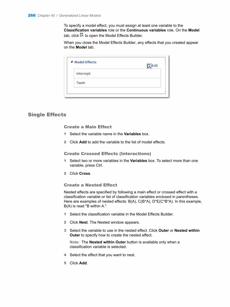
To specify a model effect, you must assign at least one variable to the Classification variables role or the Continuous variables role. On the Model tab, click to open the Model Effects Builder.
When you close the Model Effects Builder, any effects that you created appear on the Model tab.
Single Effects
Create a Main Effect
1 Select the variable name in the Variables box.
2 Click Add to add the variable to the list of model effects.
Create Crossed Effects (Interactions)
1 Select two or more variables in the Variables box. To select more than one variable, press Ctrl.
2 Click Cross.
Create a Nested Effect
Nested effects are specified by following a main effect or crossed effect with a classification variable or list of classification variables enclosed in parentheses. Here are examples of nested effects: B(A), C(B*A), D*E(C*B*A). In this example, B(A) is read "B within A."
1 Select the classification variable in the Model Effects Builder.
2 Click Nest. The Nested window appears.
3 Select the variable to use in the nested effect. Click Outer or Nested within Outer to specify how to create the nested effect.
Note: The Nested within Outer button is available only when a classification variable is selected.
4 Select the effect that you want to nest.
5 Click Add.
266 Chapter 45 / Generalized Linear Models
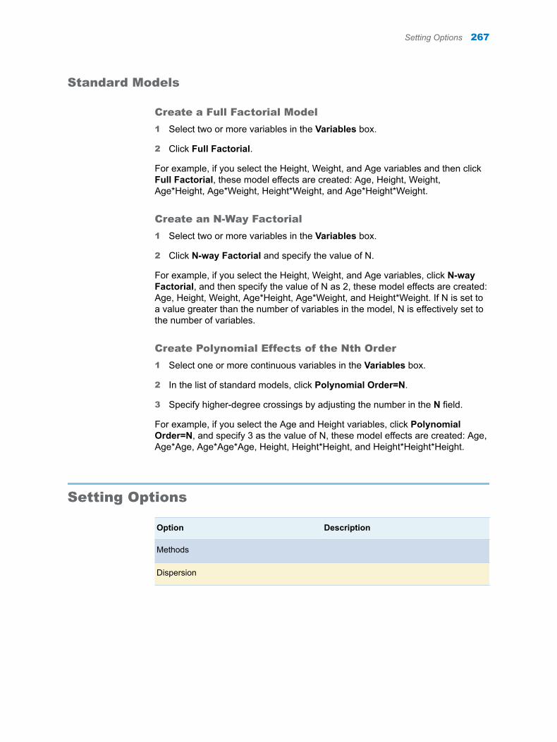
Standard Models
Create a Full Factorial Model
1 Select two or more variables in the Variables box.
2 Click Full Factorial.
For example, if you select the Height, Weight, and Age variables and then click Full Factorial, these model effects are created: Age, Height, Weight, Age*Height, Age*Weight, Height*Weight, and Age*Height*Weight.
Create an N-Way Factorial
1 Select two or more variables in the Variables box.
2 Click N-way Factorial and specify the value of N.
For example, if you select the Height, Weight, and Age variables, click N-way Factorial, and then specify the value of N as 2, these model effects are created: Age, Height, Weight, Age*Height, Age*Weight, and Height*Weight. If N is set to a value greater than the number of variables in the model, N is effectively set to the number of variables.
Create Polynomial Effects of the Nth Order
1 Select one or more continuous variables in the Variables box.
2 In the list of standard models, click Polynomial Order=N.
3 Specify higher-degree crossings by adjusting the number in the N field.
For example, if you select the Age and Height variables, click Polynomial Order=N, and specify 3 as the value of N, these model effects are created: Age, Age*Age, Age*Age*Age, Height, Height*Height, and Height*Height*Height.
Setting Options
Option Description
Methods
Dispersion
Setting Options 267

Option Description
Adjust for overdispersion adjusts the parameter covariance matrix and the likelihood function by a scale parameter. For the dispersion parameter, you can select a Pearson estimate or a deviance estimate. To define the subpopulations for calculating the Pearson and deviance chi-square goodness-of-fit tests, assign one or more variables to the role.
Note: This option is available only for binomial and multinomial distributions.
Estimate dispersion parameter enables you to specify a fixed dispersion parameter for those distributions that have a dispersion parameter. By default, this parameter is estimated.
Note: This option is not available for binomial and multinomial distributions, but it is available for the other distribution types.
Optimization
Maximum number of iterations specifies the maximum number of iterations to perform for the selected optimization technique.
Statistics
You can select the statistics to include in the output. The list of statistics depends on the selected distribution.
Here are the additional statistics that you can include:n type 1 (sequential) analysisn type 3 analysisn Wald statistics for Type 3 contrastsn confidence intervals, such as Profile likelihood confidence intervals and Wald
confidence intervalsn correlations of parameter estimatesn covariances of parameter estimatesn observation statistics, such as influence diagnostics, predicted values and
confidence intervals, and residualsn multiple comparisons for classification effectsn exact tests, which are available only for binomial distributions with a logit link
function or a Poisson distribution with a log link function.
Plots
268 Chapter 45 / Generalized Linear Models
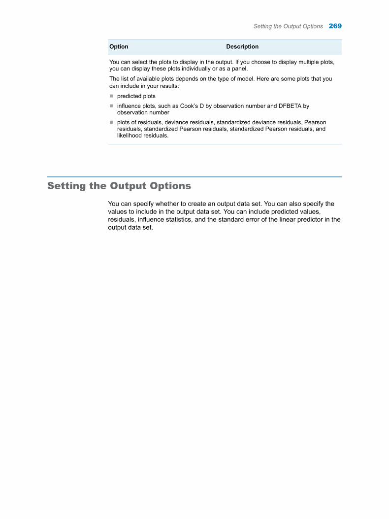
Option Description
You can select the plots to display in the output. If you choose to display multiple plots, you can display these plots individually or as a panel.
The list of available plots depends on the type of model. Here are some plots that you can include in your results:
n predicted plotsn influence plots, such as Cook’s D by observation number and DFBETA by
observation numbern plots of residuals, deviance residuals, standardized deviance residuals, Pearson
residuals, standardized Pearson residuals, standardized Pearson residuals, and likelihood residuals.
Setting the Output Options
You can specify whether to create an output data set. You can also specify the values to include in the output data set. You can include predicted values, residuals, influence statistics, and the standard error of the linear predictor in the output data set.
Setting the Output Options 269

270 Chapter 45 / Generalized Linear Models
46Mixed Models
About the Mixed Models Task . . . . . . . . . . . . . . . . . . . . . . . . . . . . . . . . . . . . . . . . . . . . . . 271
Example: Analyzing Age and Gender . . . . . . . . . . . . . . . . . . . . . . . . . . . . . . . . . . . . . . 271
Assigning Data to Roles . . . . . . . . . . . . . . . . . . . . . . . . . . . . . . . . . . . . . . . . . . . . . . . . . . . 276
Building a Model . . . . . . . . . . . . . . . . . . . . . . . . . . . . . . . . . . . . . . . . . . . . . . . . . . . . . . . . . . 277About Mixed Models . . . . . . . . . . . . . . . . . . . . . . . . . . . . . . . . . . . . . . . . . . . . . . . . . . . . . 277Single Effects . . . . . . . . . . . . . . . . . . . . . . . . . . . . . . . . . . . . . . . . . . . . . . . . . . . . . . . . . . . 280Standard Models . . . . . . . . . . . . . . . . . . . . . . . . . . . . . . . . . . . . . . . . . . . . . . . . . . . . . . . . 280
Setting the Options . . . . . . . . . . . . . . . . . . . . . . . . . . . . . . . . . . . . . . . . . . . . . . . . . . . . . . . . 281
Creating Output Data Sets . . . . . . . . . . . . . . . . . . . . . . . . . . . . . . . . . . . . . . . . . . . . . . . . . 282
About the Mixed Models Task
The Mixed Models task fits a variety of mixed linear models to data and enables you to use these fitted models to make inferences about the data. A mixed linear model is a generalization of the standard linear model. The generalization is that the data is permitted to exhibit correlation and nonconstant variability. Therefore, the mixed linear model provides the flexibility to model the means of your data (as in the standard linear model) but also the variances and covariances.
Example: Analyzing Age and Gender
1 In SAS Studio, click and select New SAS Program.
2 Create the Pr data set by copying and pasting this code into the Program tab:
data pr;input Person Gender $ y1 y2 y3 y4;y=y1; Age=8; output;y=y2; Age=10; output;y=y3; Age=12; output;y=y4; Age=14; output;drop y1-y4;
271
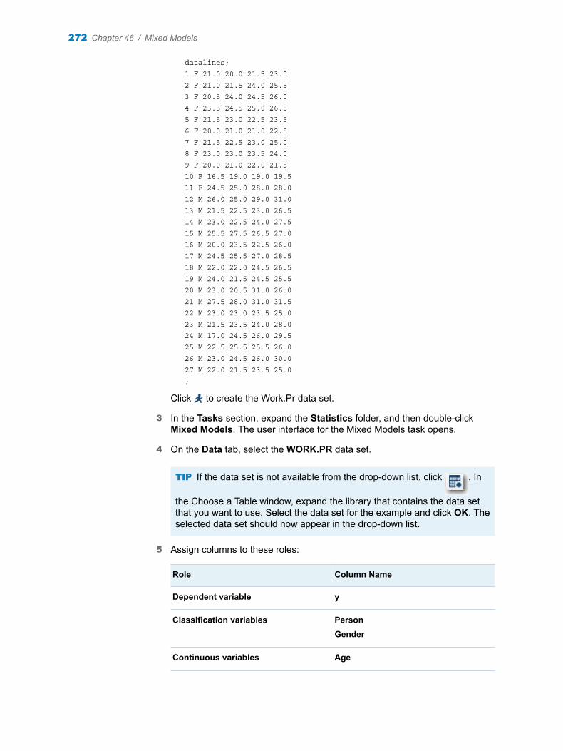
datalines;1 F 21.0 20.0 21.5 23.02 F 21.0 21.5 24.0 25.53 F 20.5 24.0 24.5 26.04 F 23.5 24.5 25.0 26.55 F 21.5 23.0 22.5 23.56 F 20.0 21.0 21.0 22.57 F 21.5 22.5 23.0 25.08 F 23.0 23.0 23.5 24.09 F 20.0 21.0 22.0 21.510 F 16.5 19.0 19.0 19.511 F 24.5 25.0 28.0 28.012 M 26.0 25.0 29.0 31.013 M 21.5 22.5 23.0 26.514 M 23.0 22.5 24.0 27.515 M 25.5 27.5 26.5 27.016 M 20.0 23.5 22.5 26.017 M 24.5 25.5 27.0 28.518 M 22.0 22.0 24.5 26.519 M 24.0 21.5 24.5 25.520 M 23.0 20.5 31.0 26.021 M 27.5 28.0 31.0 31.522 M 23.0 23.0 23.5 25.023 M 21.5 23.5 24.0 28.024 M 17.0 24.5 26.0 29.525 M 22.5 25.5 25.5 26.026 M 23.0 24.5 26.0 30.027 M 22.0 21.5 23.5 25.0;
Click to create the Work.Pr data set.
3 In the Tasks section, expand the Statistics folder, and then double-click Mixed Models. The user interface for the Mixed Models task opens.
4 On the Data tab, select the WORK.PR data set.
TIP If the data set is not available from the drop-down list, click . In
the Choose a Table window, expand the library that contains the data set that you want to use. Select the data set for the example and click OK. The selected data set should now appear in the drop-down list.
5 Assign columns to these roles:
Role Column Name
Dependent variable y
Classification variables PersonGender
Continuous variables Age
272 Chapter 46 / Mixed Models
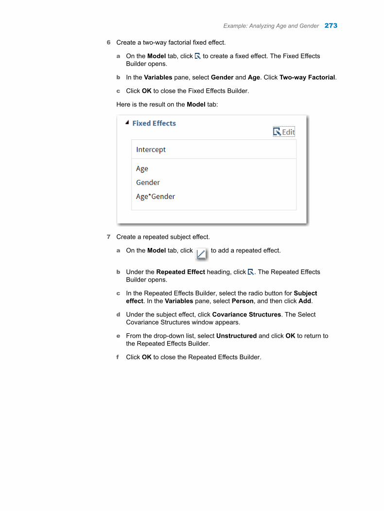
6 Create a two-way factorial fixed effect.
a On the Model tab, click to create a fixed effect. The Fixed Effects Builder opens.
b In the Variables pane, select Gender and Age. Click Two-way Factorial.
c Click OK to close the Fixed Effects Builder.
Here is the result on the Model tab:
7 Create a repeated subject effect.
a On the Model tab, click to add a repeated effect.
b Under the Repeated Effect heading, click . The Repeated Effects Builder opens.
c In the Repeated Effects Builder, select the radio button for Subject effect. In the Variables pane, select Person, and then click Add.
d Under the subject effect, click Covariance Structures. The Select Covariance Structures window appears.
e From the drop-down list, select Unstructured and click OK to return to the Repeated Effects Builder.
f Click OK to close the Repeated Effects Builder.
Example: Analyzing Age and Gender 273
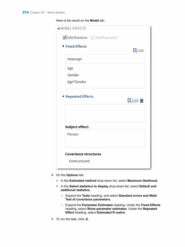
Here is the result on the Model tab:
8 On the Options tab:
n In the Estimated method drop-down list, select Maximum likelihood.
n In the Select statistics to display drop-down list, select Default and additional statistics.
o Expand the Tests heading, and select Standard errors and Wald Test of covariance parameters.
o Expand the Parameter Estimates heading. Under the Fixed Effects heading, select Show parameter estimates. Under the Repeated Effect heading, select Estimated R matrix.
9 To run the task, click .
274 Chapter 46 / Mixed Models
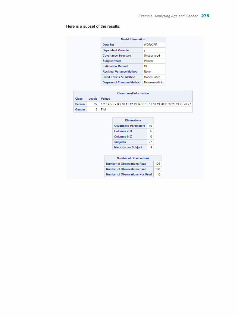
Here is a subset of the results:
Example: Analyzing Age and Gender 275
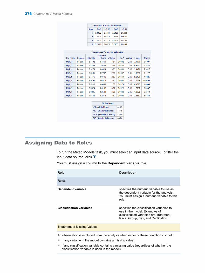
Assigning Data to Roles
To run the Mixed Models task, you must select an input data source. To filter the input data source, click .
You must assign a column to the Dependent variable role.
Role Description
Roles
Dependent variable specifies the numeric variable to use as the dependent variable for the analysis. You must assign a numeric variable to this role.
Classification variables specifies the classification variables to use in the model. Examples of classification variables are Treatment, Race, Group, Sex, and Replication.
Treatment of Missing Values
An observation is excluded from the analysis when either of these conditions is met:n if any variable in the model contains a missing valuen if any classification variable contains a missing value (regardless of whether the
classification variable is used in the model)
276 Chapter 46 / Mixed Models
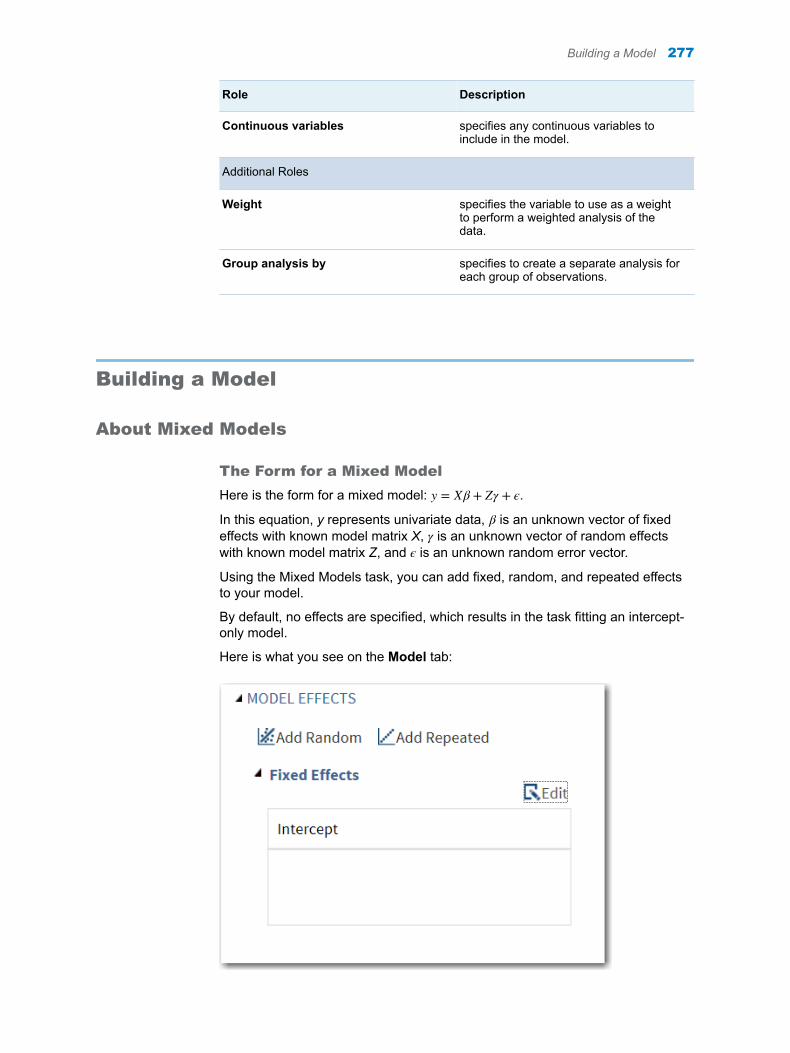
Role Description
Continuous variables specifies any continuous variables to include in the model.
Additional Roles
Weight specifies the variable to use as a weight to perform a weighted analysis of the data.
Group analysis by specifies to create a separate analysis for each group of observations.
Building a Model
About Mixed Models
The Form for a Mixed Model
Here is the form for a mixed model: y = Xβ + Zγ + ϵ.
In this equation, y represents univariate data, β is an unknown vector of fixed effects with known model matrix X, γ is an unknown vector of random effects with known model matrix Z, and ϵ is an unknown random error vector.
Using the Mixed Models task, you can add fixed, random, and repeated effects to your model.
By default, no effects are specified, which results in the task fitting an intercept-only model.
Here is what you see on the Model tab:
Building a Model 277
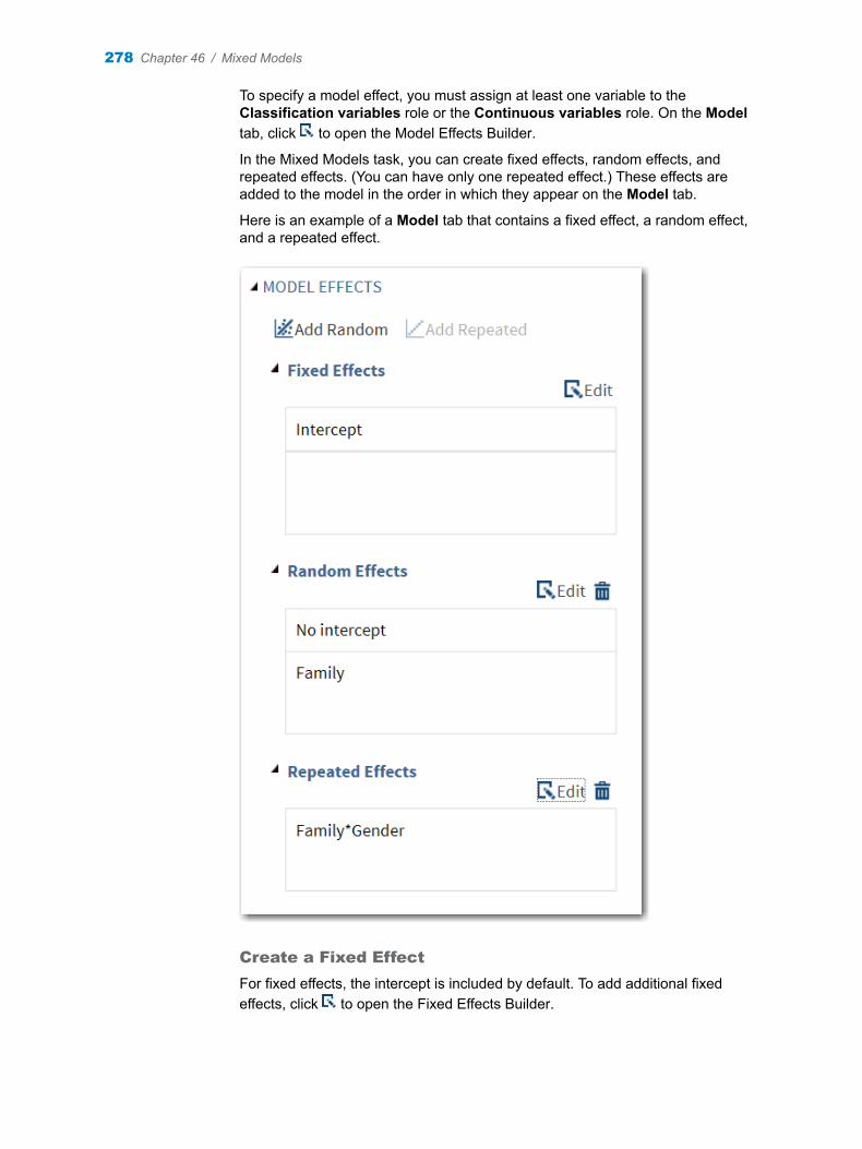
To specify a model effect, you must assign at least one variable to the Classification variables role or the Continuous variables role. On the Model tab, click to open the Model Effects Builder.
In the Mixed Models task, you can create fixed effects, random effects, and repeated effects. (You can have only one repeated effect.) These effects are added to the model in the order in which they appear on the Model tab.
Here is an example of a Model tab that contains a fixed effect, a random effect, and a repeated effect.
Create a Fixed Effect
For fixed effects, the intercept is included by default. To add additional fixed effects, click to open the Fixed Effects Builder.
278 Chapter 46 / Mixed Models
Create a Random Effect
You can have multiple random effects in the model.
To create a random effect, click to open the Random Effects Builder. In the Random Effects Builder, you can create these types of single effects: a main effect, a crossed effect, an effect with a polynomial degree of n, and a nested effect.
You can also create a subject effect or a group effect. Specifying a subject effect is equivalent to nesting all other random effects in the subject effect. The group effect is an effect that specifies heterogeneity in the covariance structure of the R matrix. All observations that have the same level of the group effect have the same covariance parameters.
To create a subject effect or group effect:
1 In the Random Effects Builder, select the variable in the Variables pane.
2 Select the radio button for Subject effect or Group effect.
3 Click the button for the single effect that you want to create.
4 For subject effects, click Covariance Structures to specify the covariance structure of the R matrix. The default covariance structure is standard variance components.
Create a Repeated Effect
You can have only one repeated effect in the model. Only classification variables can be used to create a repeated effect.
To create a repeated effect, click to open the Repeated Effects Builder. In the Repeated Effects Builder, you can create these types of single effects: a main effect, a crossed effect, an effect with a polynomial degree of n, and a nested effect. Y
You can also create a subject effect or a group effect. Specifying a subject effect is equivalent to nesting all other random effects in the subject effect. The group effect is an effect that specifies heterogeneity in the covariance structure of the R matrix. All observations that have the same level of the group effect have the same covariance parameters.
To create a subject effect or group effect:
1 In the Repeated Effects Builder, select the variable in the Variables pane.
2 Select the radio button for Subject effect or Group effect.
3 Click the button for the single effect that you want to create.
4 For subject effects, click Covariance Structures to specify the covariance structure of the R matrix. The default covariance structure is standard variance components.
Building a Model 279
Single Effects
Create a Main Effect
1 Select the variable name in the Variables box.
2 Click Add to add the variable to the list of model effects.
Create Crossed Effects (Interactions)
1 Select two or more variables in the Variables box. To select more than one variable, press Ctrl.
2 Click Cross.
Create a Polynomial Degree Effect
1 Select one or more continuous variables in the Variables box.
2 In the list of single effects, click Polynomial Degree=N.
3 Specify higher-degree crossings by adjusting the number in the N field.
For example, if you select Age, click Polynomial Degree=N, and specify 3 as the value of N, the Age*Age*Age effect is created.
Create a Nested Effect
Nested effects are specified by following a main effect or crossed effect with a classification variable or list of classification variables enclosed in parentheses. Here are examples of nested effects: B(A), C(B*A), D*E(C*B*A). In this example, B(A) is read "B within A."
1 Select the classification variable in the Model Effects Builder.
2 Click Nest. The Nested window appears.
3 Select the variable to use in the nested effect. Click Outer or Nested within Outer to specify how to create the nested effect.
Note: The Nested within Outer button is available only when a classification variable is selected.
4 Select the effect that you want to nest.
5 Click Add.
Standard Models
Create a Two-Way Factorial
1 Select two or more variables in the Variables box.
2 Click Two-Way Factorial.
280 Chapter 46 / Mixed Models
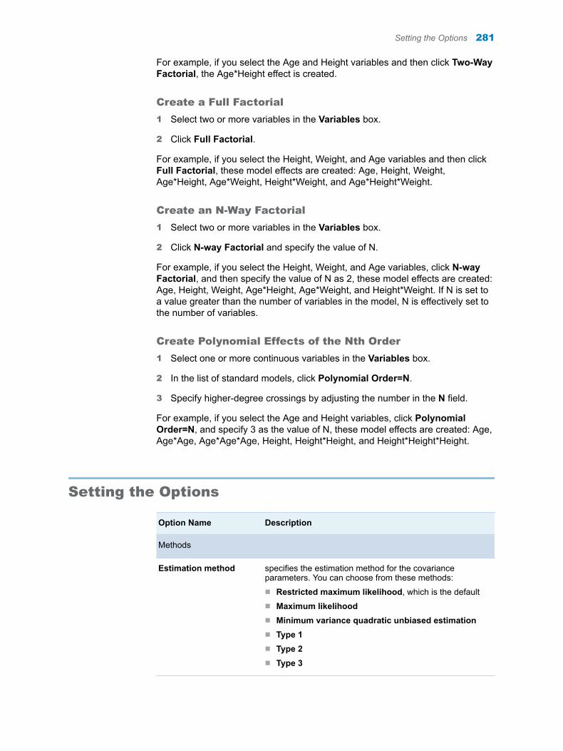
For example, if you select the Age and Height variables and then click Two-Way Factorial, the Age*Height effect is created.
Create a Full Factorial
1 Select two or more variables in the Variables box.
2 Click Full Factorial.
For example, if you select the Height, Weight, and Age variables and then click Full Factorial, these model effects are created: Age, Height, Weight, Age*Height, Age*Weight, Height*Weight, and Age*Height*Weight.
Create an N-Way Factorial
1 Select two or more variables in the Variables box.
2 Click N-way Factorial and specify the value of N.
For example, if you select the Height, Weight, and Age variables, click N-way Factorial, and then specify the value of N as 2, these model effects are created: Age, Height, Weight, Age*Height, Age*Weight, and Height*Weight. If N is set to a value greater than the number of variables in the model, N is effectively set to the number of variables.
Create Polynomial Effects of the Nth Order
1 Select one or more continuous variables in the Variables box.
2 In the list of standard models, click Polynomial Order=N.
3 Specify higher-degree crossings by adjusting the number in the N field.
For example, if you select the Age and Height variables, click Polynomial Order=N, and specify 3 as the value of N, these model effects are created: Age, Age*Age, Age*Age*Age, Height, Height*Height, and Height*Height*Height.
Setting the Options
Option Name Description
Methods
Estimation method specifies the estimation method for the covariance parameters. You can choose from these methods:n Restricted maximum likelihood, which is the defaultn Maximum likelihoodn Minimum variance quadratic unbiased estimationn Type 1n Type 2n Type 3
Setting the Options 281
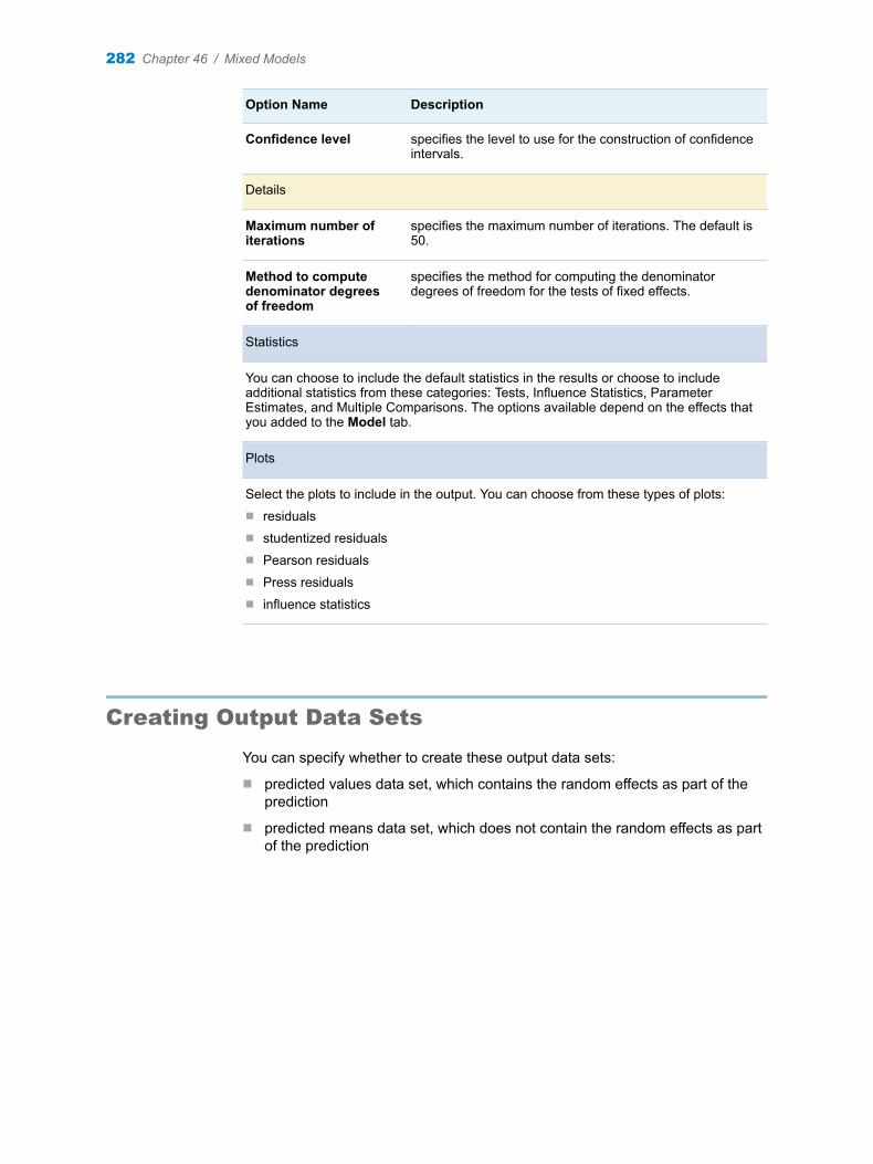
Option Name Description
Confidence level specifies the level to use for the construction of confidence intervals.
Details
Maximum number of iterations
specifies the maximum number of iterations. The default is 50.
Method to compute denominator degrees of freedom
specifies the method for computing the denominator degrees of freedom for the tests of fixed effects.
Statistics
You can choose to include the default statistics in the results or choose to include additional statistics from these categories: Tests, Influence Statistics, Parameter Estimates, and Multiple Comparisons. The options available depend on the effects that you added to the Model tab.
Plots
Select the plots to include in the output. You can choose from these types of plots:n residualsn studentized residualsn Pearson residualsn Press residualsn influence statistics
Creating Output Data Sets
You can specify whether to create these output data sets:
n predicted values data set, which contains the random effects as part of the prediction
n predicted means data set, which does not contain the random effects as part of the prediction
282 Chapter 46 / Mixed Models
47Partial Least Squares Regression
About the Partial Least Squares Regression Task . . . . . . . . . . . . . . . . . . . . . . . . . . 283
Example: Partial Least Squares Regression Analysis . . . . . . . . . . . . . . . . . . . . . . 283
Assigning Data to Roles . . . . . . . . . . . . . . . . . . . . . . . . . . . . . . . . . . . . . . . . . . . . . . . . . . . 286
Building a Model . . . . . . . . . . . . . . . . . . . . . . . . . . . . . . . . . . . . . . . . . . . . . . . . . . . . . . . . . . 287Requirements for Building a Model . . . . . . . . . . . . . . . . . . . . . . . . . . . . . . . . . . . . . . . 287Single Effects . . . . . . . . . . . . . . . . . . . . . . . . . . . . . . . . . . . . . . . . . . . . . . . . . . . . . . . . . . . 288Standard Models . . . . . . . . . . . . . . . . . . . . . . . . . . . . . . . . . . . . . . . . . . . . . . . . . . . . . . . . 289
Setting Options . . . . . . . . . . . . . . . . . . . . . . . . . . . . . . . . . . . . . . . . . . . . . . . . . . . . . . . . . . . . 290
Creating Output Data Sets . . . . . . . . . . . . . . . . . . . . . . . . . . . . . . . . . . . . . . . . . . . . . . . . . 292
About the Partial Least Squares Regression Task
The Partial Least Squares Regression task performs partial least squares analysis. It also performs principal components regression and reduced rank regression. These techniques combine dimension reduction of the predictors and dependent variables with predictive modeling.
Example: Partial Least Squares Regression Analysis
To create this example:
1 In SAS Studio, click and select New SAS Program.
2 Create the pentaTrain data set by copying and pasting this code into the Program tab.
data pentaTrain;input obsnam $ S1 L1 P1 S2 L2 P2S3 L3 P3 S4 L4 P4S5 L5 P5 log_RAI @@;
283
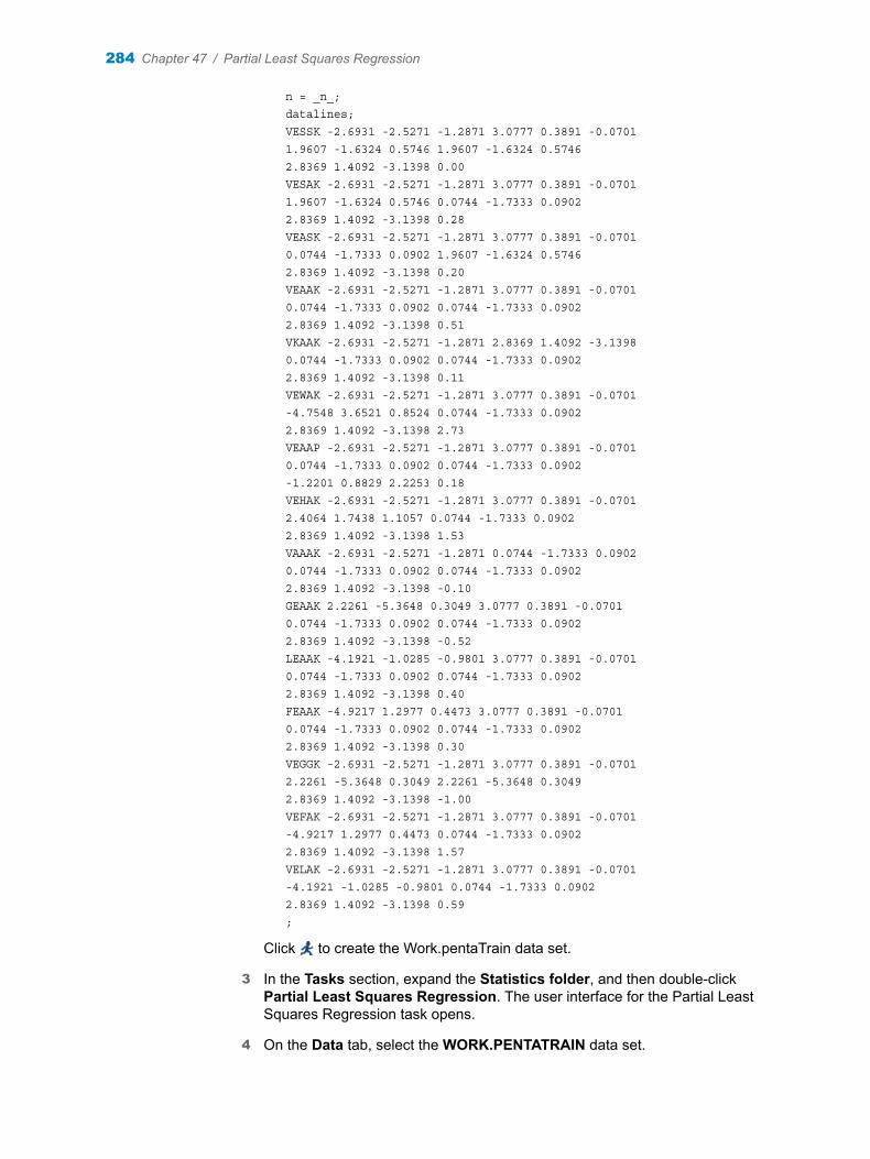
n = _n_;datalines;VESSK -2.6931 -2.5271 -1.2871 3.0777 0.3891 -0.07011.9607 -1.6324 0.5746 1.9607 -1.6324 0.57462.8369 1.4092 -3.1398 0.00VESAK -2.6931 -2.5271 -1.2871 3.0777 0.3891 -0.07011.9607 -1.6324 0.5746 0.0744 -1.7333 0.09022.8369 1.4092 -3.1398 0.28VEASK -2.6931 -2.5271 -1.2871 3.0777 0.3891 -0.07010.0744 -1.7333 0.0902 1.9607 -1.6324 0.57462.8369 1.4092 -3.1398 0.20VEAAK -2.6931 -2.5271 -1.2871 3.0777 0.3891 -0.07010.0744 -1.7333 0.0902 0.0744 -1.7333 0.09022.8369 1.4092 -3.1398 0.51VKAAK -2.6931 -2.5271 -1.2871 2.8369 1.4092 -3.13980.0744 -1.7333 0.0902 0.0744 -1.7333 0.09022.8369 1.4092 -3.1398 0.11VEWAK -2.6931 -2.5271 -1.2871 3.0777 0.3891 -0.0701-4.7548 3.6521 0.8524 0.0744 -1.7333 0.09022.8369 1.4092 -3.1398 2.73VEAAP -2.6931 -2.5271 -1.2871 3.0777 0.3891 -0.07010.0744 -1.7333 0.0902 0.0744 -1.7333 0.0902-1.2201 0.8829 2.2253 0.18VEHAK -2.6931 -2.5271 -1.2871 3.0777 0.3891 -0.07012.4064 1.7438 1.1057 0.0744 -1.7333 0.09022.8369 1.4092 -3.1398 1.53VAAAK -2.6931 -2.5271 -1.2871 0.0744 -1.7333 0.09020.0744 -1.7333 0.0902 0.0744 -1.7333 0.09022.8369 1.4092 -3.1398 -0.10GEAAK 2.2261 -5.3648 0.3049 3.0777 0.3891 -0.07010.0744 -1.7333 0.0902 0.0744 -1.7333 0.09022.8369 1.4092 -3.1398 -0.52LEAAK -4.1921 -1.0285 -0.9801 3.0777 0.3891 -0.07010.0744 -1.7333 0.0902 0.0744 -1.7333 0.09022.8369 1.4092 -3.1398 0.40FEAAK -4.9217 1.2977 0.4473 3.0777 0.3891 -0.07010.0744 -1.7333 0.0902 0.0744 -1.7333 0.09022.8369 1.4092 -3.1398 0.30VEGGK -2.6931 -2.5271 -1.2871 3.0777 0.3891 -0.07012.2261 -5.3648 0.3049 2.2261 -5.3648 0.30492.8369 1.4092 -3.1398 -1.00VEFAK -2.6931 -2.5271 -1.2871 3.0777 0.3891 -0.0701-4.9217 1.2977 0.4473 0.0744 -1.7333 0.09022.8369 1.4092 -3.1398 1.57VELAK -2.6931 -2.5271 -1.2871 3.0777 0.3891 -0.0701-4.1921 -1.0285 -0.9801 0.0744 -1.7333 0.09022.8369 1.4092 -3.1398 0.59;
Click to create the Work.pentaTrain data set.
3 In the Tasks section, expand the Statistics folder, and then double-click Partial Least Squares Regression. The user interface for the Partial Least Squares Regression task opens.
4 On the Data tab, select the WORK.PENTATRAIN data set.
284 Chapter 47 / Partial Least Squares Regression

TIP If the data set is not available from the drop-down list, click . In
the Choose a Table window, expand the library that contains the data set that you want to use. Select the data set for the example and click OK. The selected data set should now appear in the drop-down list.
5 Assign columns to these roles:
Role Column Name
Dependent variable log_RAI
Continuous variables S1–S5L1–L5P1–P5
6 On the Model tab, click . Select all of the variable names in the Variables pane and click Add.
7 To run the task, click .
Example: Partial Least Squares Regression Analysis 285
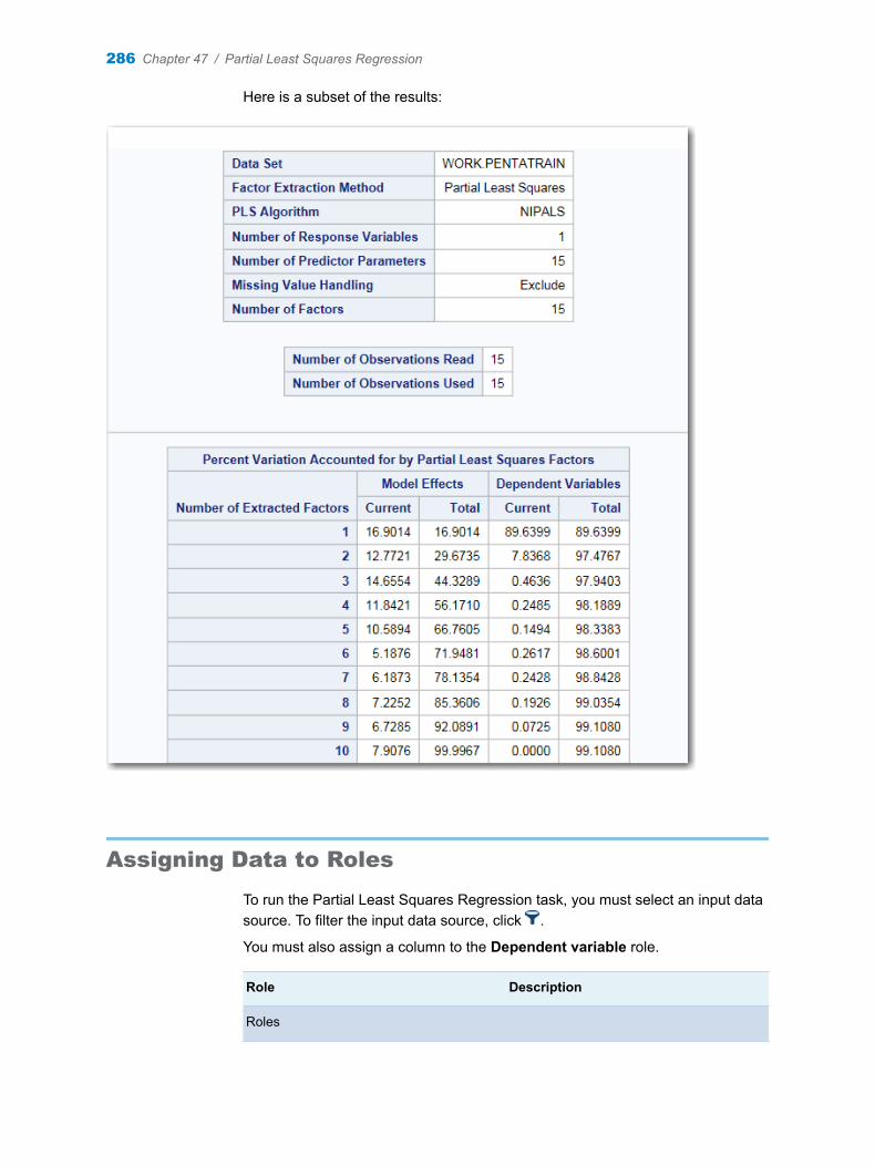
Here is a subset of the results:
Assigning Data to Roles
To run the Partial Least Squares Regression task, you must select an input data source. To filter the input data source, click .
You must also assign a column to the Dependent variable role.
Role Description
Roles
286 Chapter 47 / Partial Least Squares Regression
Role Description
Dependent variable specifies the numeric variables to use as the dependent variables for the analysis.
Classification variables specifies the classification variables to use in the model. Examples of classification variables are Treatment, Race, Group, Sex, and Replication.
Treatment of Missing Values
An observation is excluded from the analysis when either of these conditions is met:n if any variable in the model contains a missing valuen if any classification variable contains a missing value (regardless of whether the
classification variable is used in the model)
Continuous variables specifies any continuous variables to include in the model.
Additional Roles
Group analysis by specifies to create a separate analysis for each group of observations.
Building a Model
Requirements for Building a Model
By default, no effects are specified. To specify a model effect, you must assign at least one variable to the Classification variables role or the Continuous variables role. On the Model tab, click to open the Model Effects Builder.
When you close the Model Effects Builder, any effects that you created appear on the Models tab.
Building a Model 287
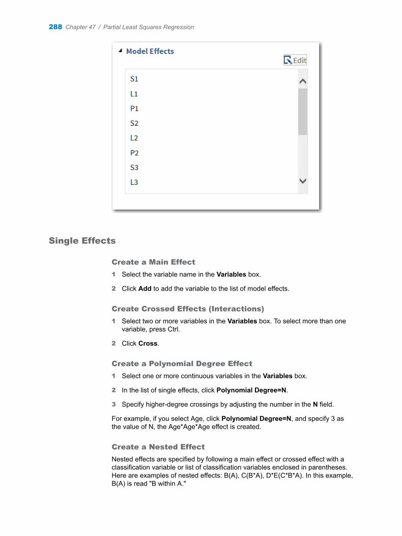
Single Effects
Create a Main Effect
1 Select the variable name in the Variables box.
2 Click Add to add the variable to the list of model effects.
Create Crossed Effects (Interactions)
1 Select two or more variables in the Variables box. To select more than one variable, press Ctrl.
2 Click Cross.
Create a Polynomial Degree Effect
1 Select one or more continuous variables in the Variables box.
2 In the list of single effects, click Polynomial Degree=N.
3 Specify higher-degree crossings by adjusting the number in the N field.
For example, if you select Age, click Polynomial Degree=N, and specify 3 as the value of N, the Age*Age*Age effect is created.
Create a Nested Effect
Nested effects are specified by following a main effect or crossed effect with a classification variable or list of classification variables enclosed in parentheses. Here are examples of nested effects: B(A), C(B*A), D*E(C*B*A). In this example, B(A) is read "B within A."
288 Chapter 47 / Partial Least Squares Regression
1 Select the classification variable in the Model Effects Builder.
2 Click Nest. The Nested window appears.
3 Select the variable to use in the nested effect. Click Outer or Nested within Outer to specify how to create the nested effect.
Note: The Nested within Outer button is available only when a classification variable is selected.
4 Select the effect that you want to nest.
5 Click Add.
Standard Models
Create a Two-Way Factorial
1 Select two or more variables in the Variables box.
2 Click Two-Way Factorial.
For example, if you select the Age and Height variables and then click Two-Way Factorial, the Age*Height effect is created.
Create a Full Factorial
1 Select two or more variables in the Variables box.
2 Click Full Factorial.
For example, if you select the Height, Weight, and Age variables and then click Full Factorial, these model effects are created: Age, Height, Weight, Age*Height, Age*Weight, Height*Weight, and Age*Height*Weight.
Create an N-Way Factorial
1 Select two or more variables in the Variables box.
2 Click N-way Factorial and specify the value of N.
For example, if you select the Height, Weight, and Age variables, click N-way Factorial, and then specify the value of N as 2, these model effects are created: Age, Height, Weight, Age*Height, Age*Weight, and Height*Weight. If N is set to a value greater than the number of variables in the model, N is effectively set to the number of variables.
Create Polynomial Effects of the Nth Order
1 Select one or more continuous variables in the Variables box.
2 In the list of standard models, click Polynomial Order=N.
3 Specify higher-degree crossings by adjusting the number in the N field.
For example, if you select the Age and Height variables, click Polynomial Order=N, and specify 3 as the value of N, these model effects are created: Age, Age*Age, Age*Age*Age, Height, Height*Height, and Height*Height*Height.
Building a Model 289
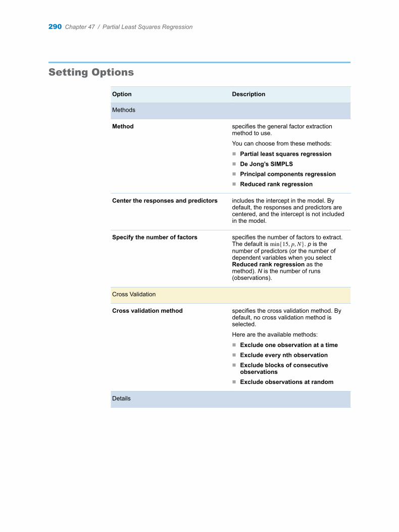
Setting Options
Option Description
Methods
Method specifies the general factor extraction method to use.
You can choose from these methods:
n Partial least squares regressionn De Jong’s SIMPLSn Principal components regressionn Reduced rank regression
Center the responses and predictors includes the intercept in the model. By default, the responses and predictors are centered, and the intercept is not included in the model.
Specify the number of factors specifies the number of factors to extract. The default is min 15, p, N . p is the number of predictors (or the number of dependent variables when you select Reduced rank regression as the method). N is the number of runs (observations).
Cross Validation
Cross validation method specifies the cross validation method. By default, no cross validation method is selected.
Here are the available methods:
n Exclude one observation at a timen Exclude every nth observationn Exclude blocks of consecutive
observationsn Exclude observations at random
Details
290 Chapter 47 / Partial Least Squares Regression
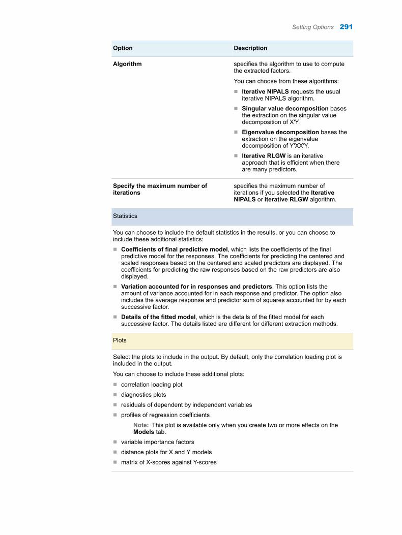
Option Description
Algorithm specifies the algorithm to use to compute the extracted factors.
You can choose from these algorithms:
n Iterative NIPALS requests the usual iterative NIPALS algorithm.
n Singular value decomposition bases the extraction on the singular value decomposition of X′Y.
n Eigenvalue decomposition bases the extraction on the eigenvalue decomposition of Y′XX′Y.
n Iterative RLGW is an iterative approach that is efficient when there are many predictors.
Specify the maximum number of iterations
specifies the maximum number of iterations if you selected the Iterative NIPALS or Iterative RLGW algorithm.
Statistics
You can choose to include the default statistics in the results, or you can choose to include these additional statistics:n Coefficients of final predictive model, which lists the coefficients of the final
predictive model for the responses. The coefficients for predicting the centered and scaled responses based on the centered and scaled predictors are displayed. The coefficients for predicting the raw responses based on the raw predictors are also displayed.
n Variation accounted for in responses and predictors. This option lists the amount of variance accounted for in each response and predictor. The option also includes the average response and predictor sum of squares accounted for by each successive factor.
n Details of the fitted model, which is the details of the fitted model for each successive factor. The details listed are different for different extraction methods.
Plots
Select the plots to include in the output. By default, only the correlation loading plot is included in the output.
You can choose to include these additional plots:
n correlation loading plotn diagnostics plotsn residuals of dependent by independent variablesn profiles of regression coefficients
Note: This plot is available only when you create two or more effects on the Models tab.
n variable importance factorsn distance plots for X and Y modelsn matrix of X-scores against Y-scores
Setting Options 291

Creating Output Data Sets
You can specify whether to create an output data set, and you can choose the statistics to include in that data set.
292 Chapter 47 / Partial Least Squares Regression

Part 5
High-Performance Statistics Tasks
Chapter 48Bin Continuous Data . . . . . . . . . . . . . . . . . . . . . . . . . . . . . . . . . . . . . . . . . . . . . 295
Chapter 49High-Performance Correlation Analysis . . . . . . . . . . . . . . . . . . . . . . . . . . . . 301
Chapter 50High-Performance Generalized Linear Models . . . . . . . . . . . . . . . . . . . . . . 305
Chapter 51Replace Missing Values . . . . . . . . . . . . . . . . . . . . . . . . . . . . . . . . . . . . . . . . . . 317
Chapter 52Random Sampling . . . . . . . . . . . . . . . . . . . . . . . . . . . . . . . . . . . . . . . . . . . . . . . 319
293

294
48Bin Continuous Data
About the Bin Continuous Data Task . . . . . . . . . . . . . . . . . . . . . . . . . . . . . . . . . . . . . . 295
Example: Winsorized Binning . . . . . . . . . . . . . . . . . . . . . . . . . . . . . . . . . . . . . . . . . . . . . 295
Assigning Data to Roles . . . . . . . . . . . . . . . . . . . . . . . . . . . . . . . . . . . . . . . . . . . . . . . . . . . 297
Setting Options . . . . . . . . . . . . . . . . . . . . . . . . . . . . . . . . . . . . . . . . . . . . . . . . . . . . . . . . . . . . 298
Creating an Output Data Set . . . . . . . . . . . . . . . . . . . . . . . . . . . . . . . . . . . . . . . . . . . . . . . 299
About the Bin Continuous Data Task
The Bin Continuous Data task is a data preparation task. This task divides the data values of a continuous variable into intervals and replaces the values for each interval with a single value that is representative of the interval.
Note: This task is available only if you are running SAS 9.4 or later and if you license and install SAS/STAT.
Example: Winsorized Binning
In this example, the task provides the basic Winsorized statistical information for the input data.
To create this example:
1 To create the Work.Ex12 data set, enter this code into a Program tab:
data ex12; length id 8; do id=1 to 10000; x1 = ranuni(101); x2 = 10*ranuni(201); x3 = 100*ranuni(301); output; end;run;
Click
295
2 In the Tasks section, expand the High-Performance Statistics folder, and then double-click Bin Continuous Data. The user interface for the Bin Continuous Data task opens.
3 On the Data tab, select the WORK.EX12 data set.
TIP If the data set is not available from the drop-down list, click . In
the Choose a Table window, expand the library that contains the data set that you want to use. Select the data set for the example and click OK. The selected data set should now appear in the drop-down list.
4 To the Variables to bin role, assign the x1 and x2 columns.
5 On the Options tab, set these options:
n In the Number of bins box, enter 10.
n From the Method drop-down list, select Winsorized binning.
6 To run the task, click .
296 Chapter 48 / Bin Continuous Data
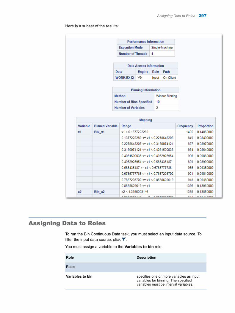
Here is a subset of the results:
Assigning Data to Roles
To run the Bin Continuous Data task, you must select an input data source. To filter the input data source, click .
You must assign a variable to the Variables to bin role.
Role Description
Roles
Variables to bin specifies one or more variables as input variables for binning. The specified variables must be interval variables.
Assigning Data to Roles 297
Role Description
Additional Roles
Frequency count lists a numeric variable whose value represents the frequency of the observation. If you assign a variable to this role, the task assumes that each observation represents n observations, where n is the value of the frequency variable. If n is not an integer, SAS truncates it. If n is less than 1 or is missing, the observation is excluded from the analysis. The sum of the frequency variable represents the total number of observations.
Setting Options
Option Name Description
Methods
Number of bins specifies the global number of binning levels for all binning variables. This value can be any integer between 2 and 1,000, inclusive. The default number of binning levels is 16.
Method specifies which binning method to use.
n Bucket binning creates equal-length bins and assigns the data to one of these bins. You can choose the number of bins during the binning. The default number of bins (the binning level) is 16.
n Winsorized binning is similar to bucket binning except that both tails are cut off to obtain a smooth binning result. This technique is often used to remove outliers during the data preparation stage.
You must specify a value for the Winsor rate option. Valid values are from 0.0 to 0.5 (exclusive). The default value is 0.05.
n Pseudo-quantile binning mimics the results of the quantile binning method but is more efficient by consuming less CPU time and memory.
Compute weight of evidence and information value
specifies whether to compute the weight of evidence and information value.
298 Chapter 48 / Bin Continuous Data
Option Name Description
Variables to bin specifies the variable to use to calculate the weight of evidence and information value. If the target variable has more than two levels, you can also specify the order of the target variable.
Specify adjustment factor specifies the adjustment factor for the weight-of-evidence calculation. You can specify a value from 0.0 to 1.0 inclusive. The default value is 0.5.
Statistics
Select statistics to display In the results, you can specify whether to include statistics.
Here are the additional statistics that you can include:n Basic statistics displays the mean,
pseudo-median, standard deviation, minimum, maximum, and number of bins for each binning variable.
n Quantile statistics displays the estimated quantiles and extremes table.
Creating an Output Data Set
You can specify whether to save the results to an output data set. In the Additional variables to include in the output data set role, specify any columns from the input data set that you want to include in the output data set.
To view all or a subset of the output data set in the results, select Show output data. This option specifies whether to display the output data set on the Results tab. You can choose to display all of the data or a subset of the output data. The task always creates an output data set that appears on the Output Data tab. The output data is also saved as a SAS data set.
Creating an Output Data Set 299

300 Chapter 48 / Bin Continuous Data
49High-Performance Correlation Analysis
About the High-Performance Correlation Analysis Task . . . . . . . . . . . . . . . . . . . . 301
Example: Correlation between Weight, Oxygen, and Run Time . . . . . . . . . . . . . 301
Assigning Data to Roles . . . . . . . . . . . . . . . . . . . . . . . . . . . . . . . . . . . . . . . . . . . . . . . . . . . 303
Setting Options . . . . . . . . . . . . . . . . . . . . . . . . . . . . . . . . . . . . . . . . . . . . . . . . . . . . . . . . . . . . 303
Creating an Output Data Set . . . . . . . . . . . . . . . . . . . . . . . . . . . . . . . . . . . . . . . . . . . . . . . 304
About the High-Performance Correlation Analysis Task
Correlation is a statistical procedure for describing the relationship between numeric variables. The relationship is described by calculating correlation coefficients for the variables. The High-Performance Correlation Analysis task computes Pearson statistics for investigating associations among variables. Correlations range from –1 to 1.
Note: This task is available only if you are running SAS 9.4 or later.
Example: Correlation between Weight, Oxygen, and Run Time
To create this example:
1 Create the Work.Fitness data set. For more information, see “FITNESS Data set” on page 588.
2 In the Tasks section, expand the High-Performance Statistics folder, and then double-click Correlation Analysis. The user interface for the High-Performance Correlation Analysis task opens.
3 On the Data tab, select the WORK.FITNESS data set.
301
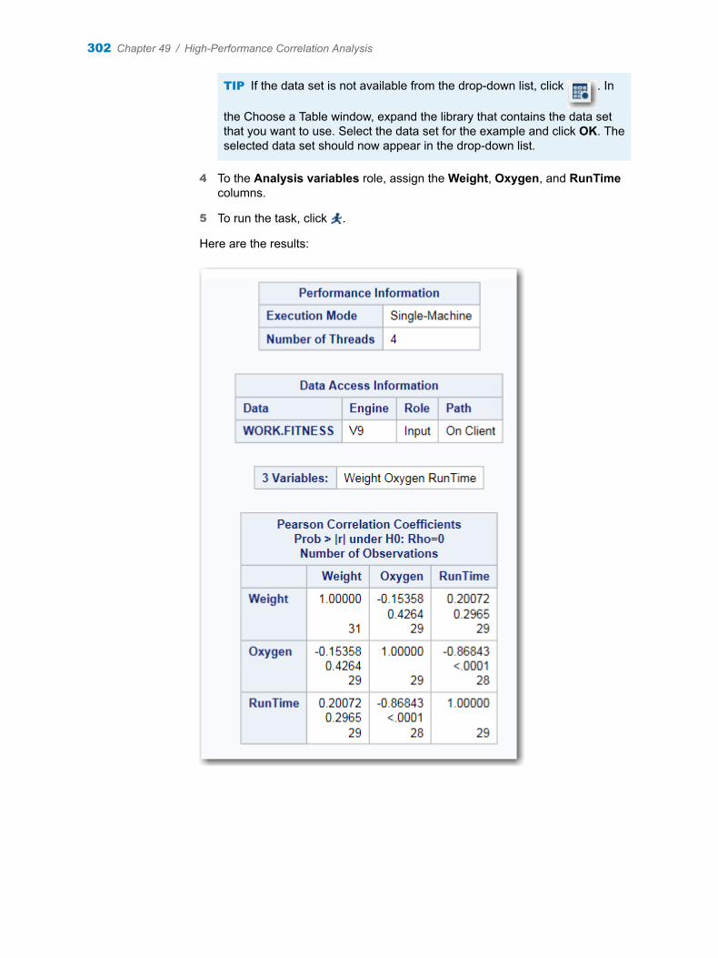
TIP If the data set is not available from the drop-down list, click . In
the Choose a Table window, expand the library that contains the data set that you want to use. Select the data set for the example and click OK. The selected data set should now appear in the drop-down list.
4 To the Analysis variables role, assign the Weight, Oxygen, and RunTime columns.
5 To run the task, click .
Here are the results:
302 Chapter 49 / High-Performance Correlation Analysis
Assigning Data to Roles
To run the High-Performance Correlation Analysis task, you must select an input data source. To filter the input data source, click .
You must assign two columns to the Analysis variables role.
Role Description
Roles
Analysis variables specifies the columns to use to calculate the correlation coefficients.
Additional Roles
Frequency count lists a numeric variable whose value represents the frequency of the observation. If you assign a variable to this role, the task assumes that each observation represents n observations, where n is the value of the frequency variable. If n is not an integer, SAS truncates it. If n is less than 1 or is missing, the observation is excluded from the analysis. The sum of the frequency variable represents the total number of observations.
Weight specifies the weights to use in the calculation of Pearson weighted product-moment correlation.
Setting Options
Option Name Description
Methods
Setting Options 303
Option Name Description
Missing values specifies whether to include missing values in the calculations.n If you select the Use nonmissing
values for all selected variables option, any observations that have missing values are excluded from the analysis.
n If you select the Use nonmissing values for pairs of variables option, the data for an observation contributes to the correlation between two variables as long as both values are nonmissing. As a result, the correlations that are calculated for the analysis variable might be based on a different number of observations.
Statistics
You can specify whether the results include only the statistics that the task automatically generates, the statistics that you selected, or no statistics. By default, only the correlations table is displayed in the results.
You can include these statistics in the results:n correlationsn covariancesn sum of squares and cross-productsn corrected sum of squares and cross-productsn descriptive statistics
Display p-values specifies whether to display for each correlation coefficient the probability of observing a more extreme value than the observed coefficient.
Order correlations from highest to lowest (in absolute value)
displays the ordered correlation coefficients for each variable. Correlations are ordered from highest to lowest in absolute value.
Creating an Output Data Set
You can specify whether to save the results to an output data set. By default, the output data set contains the correlations. You can also include covariances, sum of squares and cross-products, and corrected sum of squares and cross-products.
304 Chapter 49 / High-Performance Correlation Analysis
50High-Performance Generalized Linear Models
About the Generalized Linear Models Task . . . . . . . . . . . . . . . . . . . . . . . . . . . . . . . . 305
Example: Model Selection . . . . . . . . . . . . . . . . . . . . . . . . . . . . . . . . . . . . . . . . . . . . . . . . . 305
Partitioning Data . . . . . . . . . . . . . . . . . . . . . . . . . . . . . . . . . . . . . . . . . . . . . . . . . . . . . . . . . . 307
Assigning Data to Roles . . . . . . . . . . . . . . . . . . . . . . . . . . . . . . . . . . . . . . . . . . . . . . . . . . . 308
Building a Model . . . . . . . . . . . . . . . . . . . . . . . . . . . . . . . . . . . . . . . . . . . . . . . . . . . . . . . . . . 311Requirements for Building a Model . . . . . . . . . . . . . . . . . . . . . . . . . . . . . . . . . . . . . . . 311Single Effects . . . . . . . . . . . . . . . . . . . . . . . . . . . . . . . . . . . . . . . . . . . . . . . . . . . . . . . . . . . 312Standard Models . . . . . . . . . . . . . . . . . . . . . . . . . . . . . . . . . . . . . . . . . . . . . . . . . . . . . . . . 313
Setting the Model Selection Options . . . . . . . . . . . . . . . . . . . . . . . . . . . . . . . . . . . . . . . 314
Setting Options . . . . . . . . . . . . . . . . . . . . . . . . . . . . . . . . . . . . . . . . . . . . . . . . . . . . . . . . . . . . 316
Setting the Output Options . . . . . . . . . . . . . . . . . . . . . . . . . . . . . . . . . . . . . . . . . . . . . . . . 316
About the Generalized Linear Models Task
The Generalized Linear Models task is a high-performance task that provides model fitting and model building for generalized linear models. The task fits models for standard distributions such as Normal, Poisson, and Tweedie in the exponential family. This task also fits multinomial models for ordinal and nominal responses and provides forward, backward, and stepwise selection methods.
Note: This task is available only if you are running SAS 9.4 or later and if you license and install SAS/STAT.
Example: Model Selection
To create this example:
1 Create the Work.getStarted data set. For more information, see “GETSTARTED Data Set” on page 589.
305
2 In the Tasks section, expand the High-Performance Statistics folder, and then double-click Generalized Linear Models. The user interface for the Generalized Linear Models task opens.
3 On the Data tab, select the WORK.GETSTARTED data set.
TIP If the data set is not available from the drop-down list, click . In
the Choose a Table window, expand the library that contains the data set that you want to use. Select the data set for the example and click OK. The selected data set should now appear in the drop-down list.
4 Assign columns to these roles:
Role or Option Name Column Name
Distribution Poisson
Response variable Y
Classification variables C1C2C3C4C5
5 On the Models tab, click to open the Model Effects Builder.
6 In the Variables box, select C1–C5.
7 Click Add. Then click OK to close the Model Effects Builder.
8 Click the Selection tab. From the Selection method drop-down list, select Forward selection.
9 To run the task, click .
306 Chapter 50 / High-Performance Generalized Linear Models
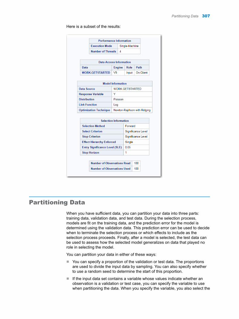
Here is a subset of the results:
Partitioning Data
When you have sufficient data, you can partition your data into three parts: training data, validation data, and test data. During the selection process, models are fit on the training data, and the prediction error for the model is determined using the validation data. This prediction error can be used to decide when to terminate the selection process or which effects to include as the selection process proceeds. Finally, after a model is selected, the test data can be used to assess how the selected model generalizes on data that played no role in selecting the model.
You can partition your data in either of these ways:
n You can specify a proportion of the validation or test data. The proportions are used to divide the input data by sampling. You can also specify whether to use a random seed to determine the start of this proportion.
n If the input data set contains a variable whose values indicate whether an observation is a validation or test case, you can specify the variable to use when partitioning the data. When you specify the variable, you also select the
Partitioning Data 307
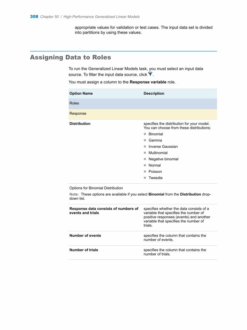
appropriate values for validation or test cases. The input data set is divided into partitions by using these values.
Assigning Data to Roles
To run the Generalized Linear Models task, you must select an input data source. To filter the input data source, click .
You must assign a column to the Response variable role.
Option Name Description
Roles
Response
Distribution specifies the distribution for your model. You can choose from these distributions:n Binomialn Gamman Inverse Gaussiann Multinomialn Negative binomialn Normaln Poissonn Tweedie
Options for Binomial Distribution
Note: These options are available if you select Binomial from the Distribution drop-down list.
Response data consists of numbers of events and trials
specifies whether the data consists of a variable that specifies the number of positive responses (events) and another variable that specifies the number of trials.
Number of events specifies the column that contains the number of events.
Number of trials specifies the column that contains the number of trials.
308 Chapter 50 / High-Performance Generalized Linear Models
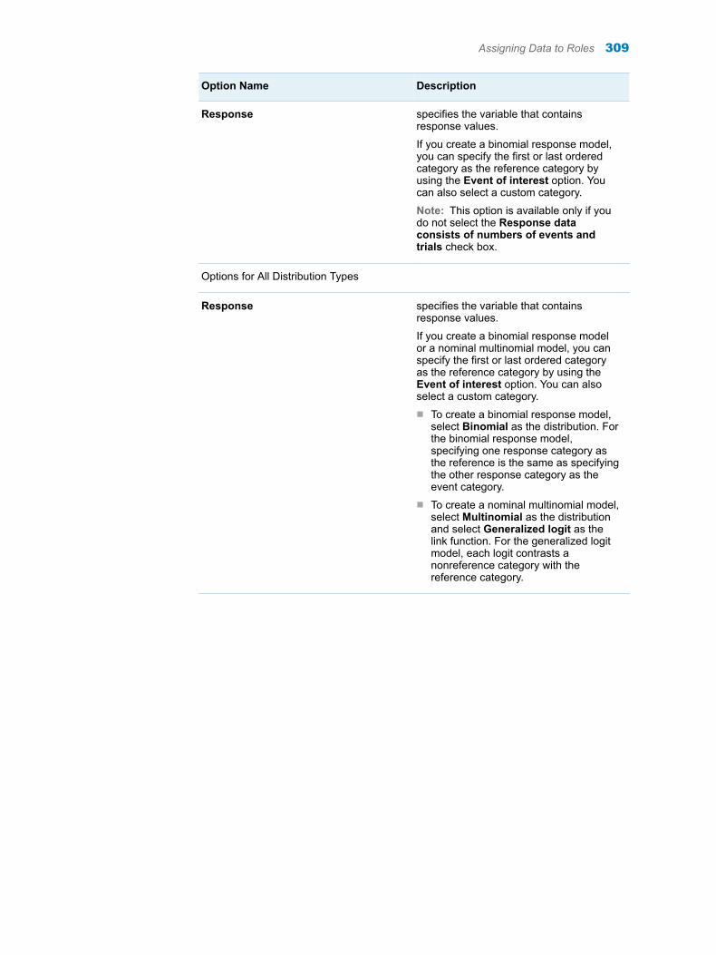
Option Name Description
Response specifies the variable that contains response values.
If you create a binomial response model, you can specify the first or last ordered category as the reference category by using the Event of interest option. You can also select a custom category.
Note: This option is available only if you do not select the Response data consists of numbers of events and trials check box.
Options for All Distribution Types
Response specifies the variable that contains response values.
If you create a binomial response model or a nominal multinomial model, you can specify the first or last ordered category as the reference category by using the Event of interest option. You can also select a custom category.n To create a binomial response model,
select Binomial as the distribution. For the binomial response model, specifying one response category as the reference is the same as specifying the other response category as the event category.
n To create a nominal multinomial model, select Multinomial as the distribution and select Generalized logit as the link function. For the generalized logit model, each logit contrasts a nonreference category with the reference category.
Assigning Data to Roles 309
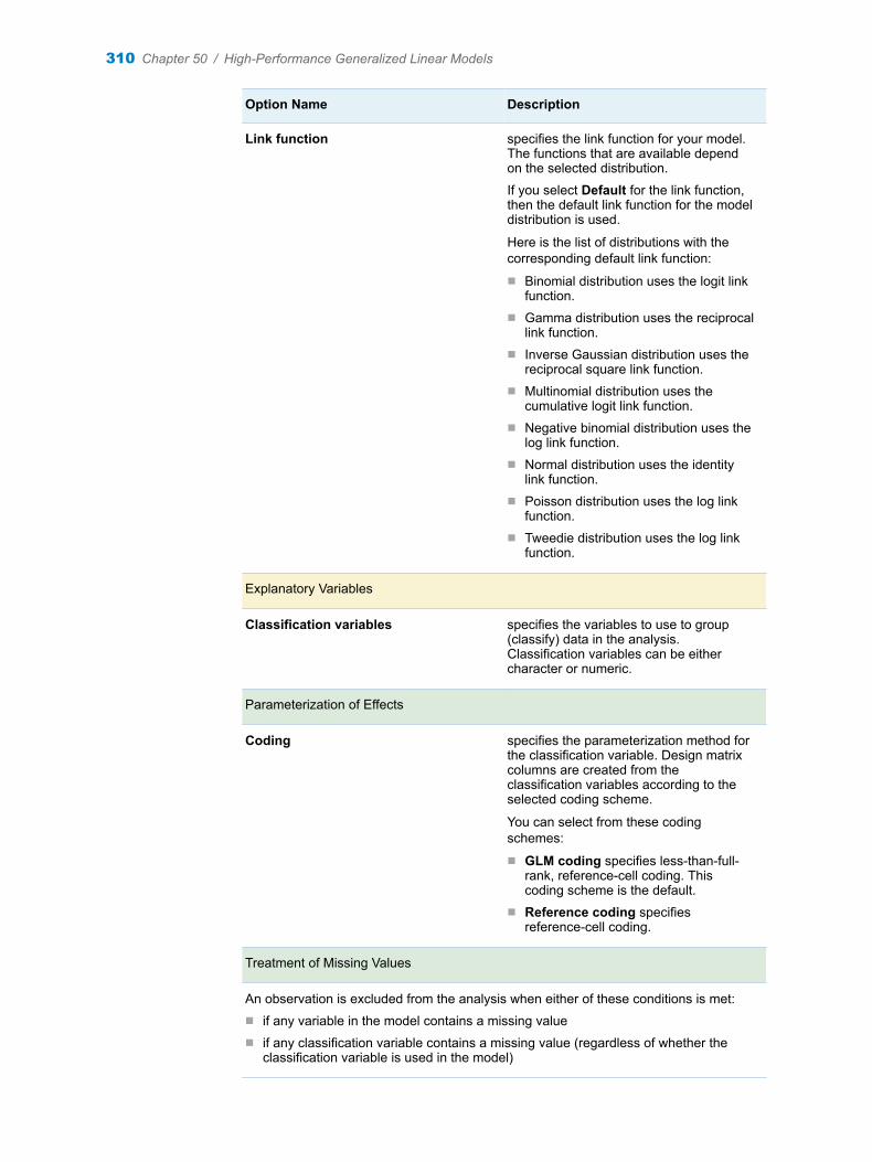
Option Name Description
Link function specifies the link function for your model. The functions that are available depend on the selected distribution.
If you select Default for the link function, then the default link function for the model distribution is used.
Here is the list of distributions with the corresponding default link function:
n Binomial distribution uses the logit link function.
n Gamma distribution uses the reciprocal link function.
n Inverse Gaussian distribution uses the reciprocal square link function.
n Multinomial distribution uses the cumulative logit link function.
n Negative binomial distribution uses the log link function.
n Normal distribution uses the identity link function.
n Poisson distribution uses the log link function.
n Tweedie distribution uses the log link function.
Explanatory Variables
Classification variables specifies the variables to use to group (classify) data in the analysis. Classification variables can be either character or numeric.
Parameterization of Effects
Coding specifies the parameterization method for the classification variable. Design matrix columns are created from the classification variables according to the selected coding scheme.
You can select from these coding schemes:
n GLM coding specifies less-than-full-rank, reference-cell coding. This coding scheme is the default.
n Reference coding specifies reference-cell coding.
Treatment of Missing Values
An observation is excluded from the analysis when either of these conditions is met:n if any variable in the model contains a missing valuen if any classification variable contains a missing value (regardless of whether the
classification variable is used in the model)
310 Chapter 50 / High-Performance Generalized Linear Models
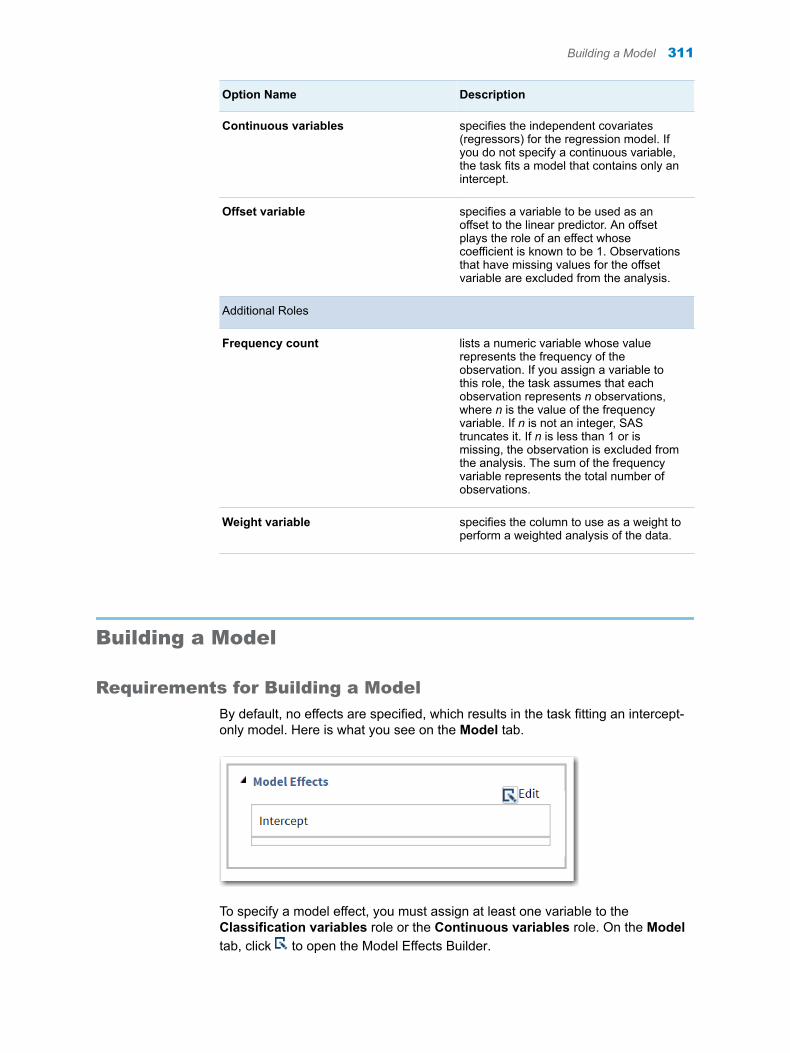
Option Name Description
Continuous variables specifies the independent covariates (regressors) for the regression model. If you do not specify a continuous variable, the task fits a model that contains only an intercept.
Offset variable specifies a variable to be used as an offset to the linear predictor. An offset plays the role of an effect whose coefficient is known to be 1. Observations that have missing values for the offset variable are excluded from the analysis.
Additional Roles
Frequency count lists a numeric variable whose value represents the frequency of the observation. If you assign a variable to this role, the task assumes that each observation represents n observations, where n is the value of the frequency variable. If n is not an integer, SAS truncates it. If n is less than 1 or is missing, the observation is excluded from the analysis. The sum of the frequency variable represents the total number of observations.
Weight variable specifies the column to use as a weight to perform a weighted analysis of the data.
Building a Model
Requirements for Building a Model
By default, no effects are specified, which results in the task fitting an intercept-only model. Here is what you see on the Model tab.
To specify a model effect, you must assign at least one variable to the Classification variables role or the Continuous variables role. On the Model tab, click to open the Model Effects Builder.
Building a Model 311
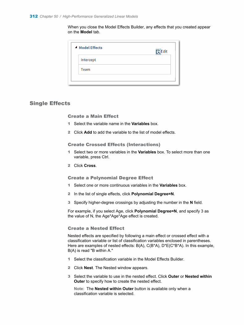
When you close the Model Effects Builder, any effects that you created appear on the Model tab.
Single Effects
Create a Main Effect
1 Select the variable name in the Variables box.
2 Click Add to add the variable to the list of model effects.
Create Crossed Effects (Interactions)
1 Select two or more variables in the Variables box. To select more than one variable, press Ctrl.
2 Click Cross.
Create a Polynomial Degree Effect
1 Select one or more continuous variables in the Variables box.
2 In the list of single effects, click Polynomial Degree=N.
3 Specify higher-degree crossings by adjusting the number in the N field.
For example, if you select Age, click Polynomial Degree=N, and specify 3 as the value of N, the Age*Age*Age effect is created.
Create a Nested Effect
Nested effects are specified by following a main effect or crossed effect with a classification variable or list of classification variables enclosed in parentheses. Here are examples of nested effects: B(A), C(B*A), D*E(C*B*A). In this example, B(A) is read "B within A."
1 Select the classification variable in the Model Effects Builder.
2 Click Nest. The Nested window appears.
3 Select the variable to use in the nested effect. Click Outer or Nested within Outer to specify how to create the nested effect.
Note: The Nested within Outer button is available only when a classification variable is selected.
312 Chapter 50 / High-Performance Generalized Linear Models
4 Select the effect that you want to nest.
5 Click Add.
Standard Models
Create a Two-Way Factorial
1 Select two or more variables in the Variables box.
2 Click Two-Way Factorial.
For example, if you select the Age and Height variables and then click Two-Way Factorial, the Age*Height effect is created.
Create a Full Factorial
1 Select two or more variables in the Variables box.
2 Click Full Factorial.
For example, if you select the Height, Weight, and Age variables and then click Full Factorial, these model effects are created: Age, Height, Weight, Age*Height, Age*Weight, Height*Weight, and Age*Height*Weight.
Create an N-Way Factorial
1 Select two or more variables in the Variables box.
2 Click N-way Factorial and specify the value of N.
For example, if you select the Height, Weight, and Age variables, click N-way Factorial, and then specify the value of N as 2, these model effects are created: Age, Height, Weight, Age*Height, Age*Weight, and Height*Weight. If N is set to a value greater than the number of variables in the model, N is effectively set to the number of variables.
Create Polynomial Effects of the Nth Order
1 Select one or more continuous variables in the Variables box.
2 In the list of standard models, click Polynomial Order=N.
3 Specify higher-degree crossings by adjusting the number in the N field.
For example, if you select the Age and Height variables, click Polynomial Order=N, and specify 3 as the value of N, these model effects are created: Age, Age*Age, Age*Age*Age, Height, Height*Height, and Height*Height*Height.
Building a Model 313
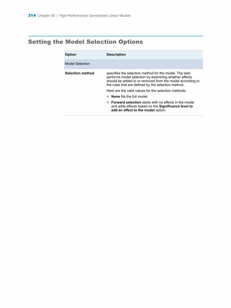
Setting the Model Selection Options
Option Description
Model Selection
Selection method specifies the selection method for the model. The task performs model selection by examining whether effects should be added to or removed from the model according to the rules that are defined by the selection method.
Here are the valid values for the selection methods:n None fits the full model.n Forward selection starts with no effects in the model
and adds effects based on the Significance level to add an effect to the model option.
314 Chapter 50 / High-Performance Generalized Linear Models
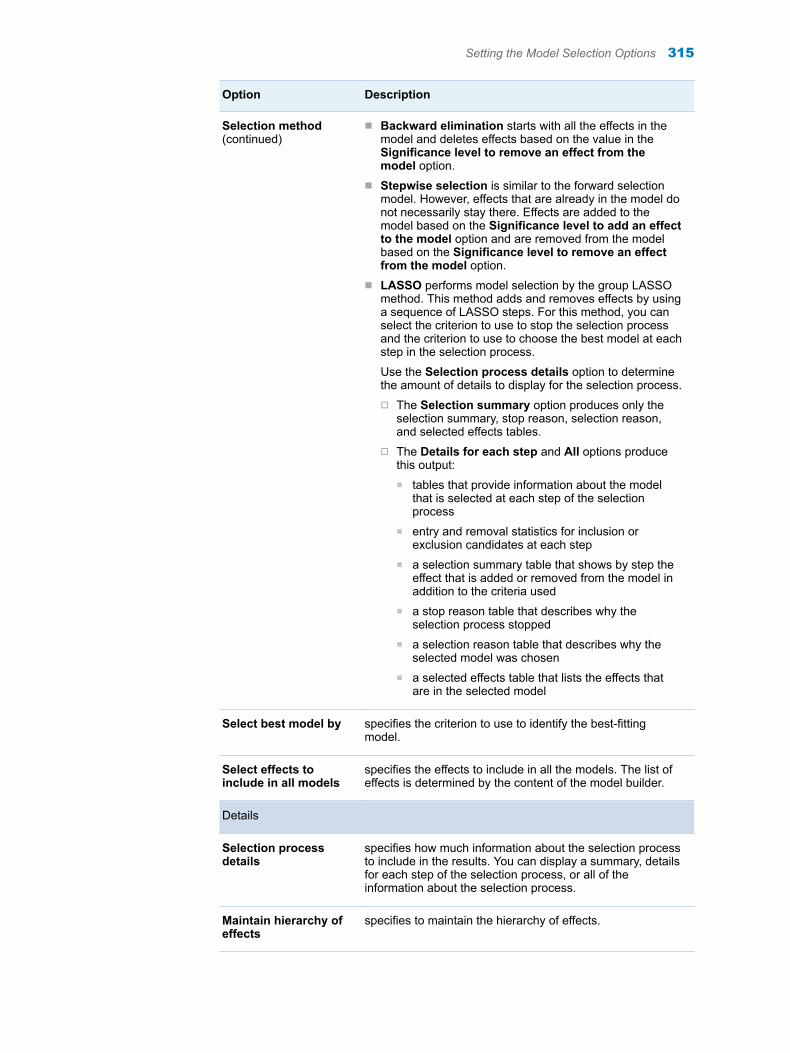
Option Description
Selection method (continued)
n Backward elimination starts with all the effects in the model and deletes effects based on the value in the Significance level to remove an effect from the model option.
n Stepwise selection is similar to the forward selection model. However, effects that are already in the model do not necessarily stay there. Effects are added to the model based on the Significance level to add an effect to the model option and are removed from the model based on the Significance level to remove an effect from the model option.
n LASSO performs model selection by the group LASSO method. This method adds and removes effects by using a sequence of LASSO steps. For this method, you can select the criterion to use to stop the selection process and the criterion to use to choose the best model at each step in the selection process.
Use the Selection process details option to determine the amount of details to display for the selection process.o The Selection summary option produces only the
selection summary, stop reason, selection reason, and selected effects tables.
o The Details for each step and All options produce this output:n tables that provide information about the model
that is selected at each step of the selection process
n entry and removal statistics for inclusion or exclusion candidates at each step
n a selection summary table that shows by step the effect that is added or removed from the model in addition to the criteria used
n a stop reason table that describes why the selection process stopped
n a selection reason table that describes why the selected model was chosen
n a selected effects table that lists the effects that are in the selected model
Select best model by specifies the criterion to use to identify the best-fitting model.
Select effects to include in all models
specifies the effects to include in all the models. The list of effects is determined by the content of the model builder.
Details
Selection process details
specifies how much information about the selection process to include in the results. You can display a summary, details for each step of the selection process, or all of the information about the selection process.
Maintain hierarchy of effects
specifies to maintain the hierarchy of effects.
Setting the Model Selection Options 315
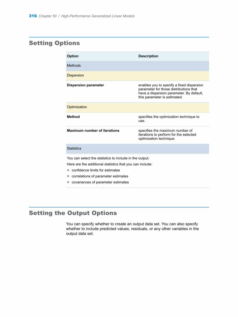
Setting Options
Option Description
Methods
Dispersion
Dispersion parameter enables you to specify a fixed dispersion parameter for those distributions that have a dispersion parameter. By default, this parameter is estimated.
Optimization
Method specifies the optimization technique to use.
Maximum number of iterations specifies the maximum number of iterations to perform for the selected optimization technique.
Statistics
You can select the statistics to include in the output.
Here are the additional statistics that you can include:n confidence limits for estimatesn correlations of parameter estimatesn covariances of parameter estimates
Setting the Output Options
You can specify whether to create an output data set. You can also specify whether to include predicted values, residuals, or any other variables in the output data set.
316 Chapter 50 / High-Performance Generalized Linear Models

51Replace Missing Values
About the Replace Missing Values Task . . . . . . . . . . . . . . . . . . . . . . . . . . . . . . . . . . . 317
Assigning Data to Roles . . . . . . . . . . . . . . . . . . . . . . . . . . . . . . . . . . . . . . . . . . . . . . . . . . . 317
Setting the Output Options . . . . . . . . . . . . . . . . . . . . . . . . . . . . . . . . . . . . . . . . . . . . . . . . 318
About the Replace Missing Values Task
The Replace Missing Values task replaces missing values in a data set with an estimate of the missing value. The task also creates binary imputation indicators.
Note: You must license and install SAS/STAT to use this task.
Assigning Data to Roles
To run the Replace Missing Values task, you must select an input data source. To filter the input data source, click .
Role Description
Roles
Replace missing values with the mean replaces missing values with the mean for the variable.
Replace missing values with the pseudo-median
replaces missing values with the pseudo-median of the variable. If there is no nonmissing value, the pseudo-median is 0.
Replace missing values with a random number
replaces missing values with a random value that is drawn between the minimum and maximum of the variable. If there is no nonmissing value, the random value is 0.
Additional Roles
317
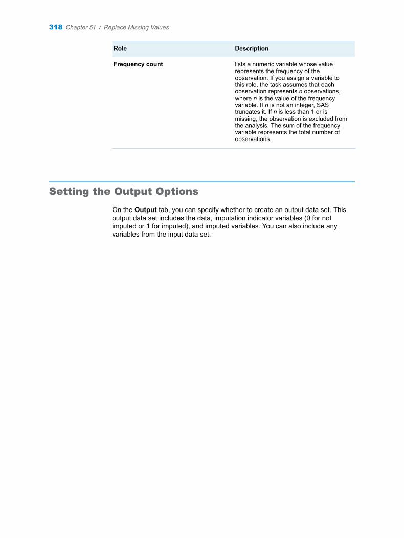
Role Description
Frequency count lists a numeric variable whose value represents the frequency of the observation. If you assign a variable to this role, the task assumes that each observation represents n observations, where n is the value of the frequency variable. If n is not an integer, SAS truncates it. If n is less than 1 or is missing, the observation is excluded from the analysis. The sum of the frequency variable represents the total number of observations.
Setting the Output Options
On the Output tab, you can specify whether to create an output data set. This output data set includes the data, imputation indicator variables (0 for not imputed or 1 for imputed), and imputed variables. You can also include any variables from the input data set.
318 Chapter 51 / Replace Missing Values
52Random Sampling
About the Random Sampling Task . . . . . . . . . . . . . . . . . . . . . . . . . . . . . . . . . . . . . . . . . 319
Assigning Data to Roles . . . . . . . . . . . . . . . . . . . . . . . . . . . . . . . . . . . . . . . . . . . . . . . . . . . 319
Creating the Output Data Set . . . . . . . . . . . . . . . . . . . . . . . . . . . . . . . . . . . . . . . . . . . . . . 320
Setting Options . . . . . . . . . . . . . . . . . . . . . . . . . . . . . . . . . . . . . . . . . . . . . . . . . . . . . . . . . . . . 321
About the Random Sampling Task
The Random Sampling task is a high-performance procedure that performs either simple random sampling or stratified sampling. The output from this task includes an output data set and the sample data, a table with performance information, and a table with frequency information for the population and sample.
Note: This task is available only if you are running SAS 9.4 or later and if you license and install SAS/STAT.
Assigning Data to Roles
To run the Random Sampling task, you must select an input data set. To filter the input data source, click .
319
If you want to perform stratified sampling, you must assign a column to the Stratify by role. Otherwise, the Stratify by role is optional.
Role Description
Stratify by specifies the variables to use to partition the input table into mutually exclusive, nonoverlapping subsets that are known as strata. Each stratum is defined by a set of values of the strata variables, and each stratum is sampled separately. The complete sample is the union of the samples that are taken from all the strata.
Note: If you do not assign any variables to this role, then the entire input table is treated as a single stratum.
You can allocate the total sample size among the strata in proportion to the size of the stratum. For example, the variable GENDER has possible values of M and F, and the variable VOTED has possible values of Y and N. If you assign both GENDER and VOTED to the Stratify by role, then the input table is partitioned into four strata: males who voted, males who did not vote, females who voted, and females who did not vote.
The input table contains 20,000 rows, and the values are distributed as follows:
n 7,000 males who votedn 4,000 males who did not vote n 5,000 females who voted n 4,000 females who did not vote
Therefore, the proportion of males who voted is 7,000/20,000=0.35 or 35%. The proportions in the sample should reflect the proportions of the strata in the input table. For example, if your sample table contains 100 observations, then 35% of the values in the sample must be selected from the males who voted stratum to reflect the proportions in the input table.
Ignore case of character stratification values
distinguishes stratified variables that share the same normalized value when you perform stratified sampling. For example, if a target has three distinct values, “A”, “B”, and “b”, and you want to treat “B” and “b” as different levels, you need to select this option. Otherwise, “B” and “b” are treated as the same level. The task normalizes a value as follows:
1 Leading blanks are removed.
2 The value is truncated to 32 characters.
3 Letters are changed from lowercase to uppercase.
Creating the Output Data Set
On the Data tab, you can select the numeric and character variables from the input data set to include in the output data. Select the Include all input observations and a sampling indicator variable to produce an output table with the same number of rows as the input table. The output table has an
320 Chapter 52 / Random Sampling
additional partition indicator (_PARTIND_) to indicate whether an observation is included in the sample (1) or not (0).
The Show output data option specifies whether to display the output data set on the Results tab. You can choose to display all of the data or a subset of the output data. The task always creates an output data set that appears on the Output Data tab. The output data is also saved as a SAS data set.
Setting Options
Option Name Description
Methods
Sample by specifies the sample size in the desired number of rows or in the desired percentage of input rows. For example, if you specify 3% of rows and there are 400 input rows, then the resulting sample has 12 rows.
Note: If you assign variables to the Stratify by role, then the sample size specification that you make here applies to each stratum rather than to the entire input table.
Specify the random seed specifies the initial seed for the generation of random numbers. If you set this value to zero or a negative number, then a seed that is based on the system clock is used to produce the sample.
Setting Options 321

322 Chapter 52 / Random Sampling
Part 6
Power and Sample Size
Chapter 53Pearson Correlation . . . . . . . . . . . . . . . . . . . . . . . . . . . . . . . . . . . . . . . . . . . . . 325
Chapter 54Multiple Regression . . . . . . . . . . . . . . . . . . . . . . . . . . . . . . . . . . . . . . . . . . . . . 329
Chapter 55Confidence Intervals . . . . . . . . . . . . . . . . . . . . . . . . . . . . . . . . . . . . . . . . . . . . . 333
Chapter 56Tests of Proportions . . . . . . . . . . . . . . . . . . . . . . . . . . . . . . . . . . . . . . . . . . . . . 337
Chapter 57t Tests . . . . . . . . . . . . . . . . . . . . . . . . . . . . . . . . . . . . . . . . . . . . . . . . . . . . . . . . . 341
Chapter 58Cox Regression . . . . . . . . . . . . . . . . . . . . . . . . . . . . . . . . . . . . . . . . . . . . . . . . . 345
323

324
53Pearson Correlation
About the Pearson Correlation Task . . . . . . . . . . . . . . . . . . . . . . . . . . . . . . . . . . . . . . . 325
Example: Pearson Correlation for Power and Sample Size Analysis . . . . . . . . 325
Assigning Properties . . . . . . . . . . . . . . . . . . . . . . . . . . . . . . . . . . . . . . . . . . . . . . . . . . . . . . 326
Setting the Plot Options . . . . . . . . . . . . . . . . . . . . . . . . . . . . . . . . . . . . . . . . . . . . . . . . . . . 328
About the Pearson Correlation Task
Power and sample size analysis optimizes the resource usage and design of a study, which improves the chances of conclusive results with maximum efficiency. This task performs power and sample size analyses for tests of simple and partial Pearson correlation between two variables. Both Fisher’s z transformation and the t transformation are supported.
Example: Pearson Correlation for Power and Sample Size Analysis
To create this example:
1 In the Tasks section, expand the Power and Sample Size folder, and then double-click Pearson Correlation. The user interface for the Pearson Correlation task opens.
2 Under the Solve For heading, select Power.
3 For the analysis test, select Fisher’s z transformation.
4 For the number of sides, select Two-sided test.
5 Specify a significance level of 0.05.
6 Under the Correlation heading, select Correlation, Null correlation from the Select a form drop-down list.
7 Enter .3 as the correlation, and enter .1 as the null correlation.
8 For the sample size, enter 180.
325
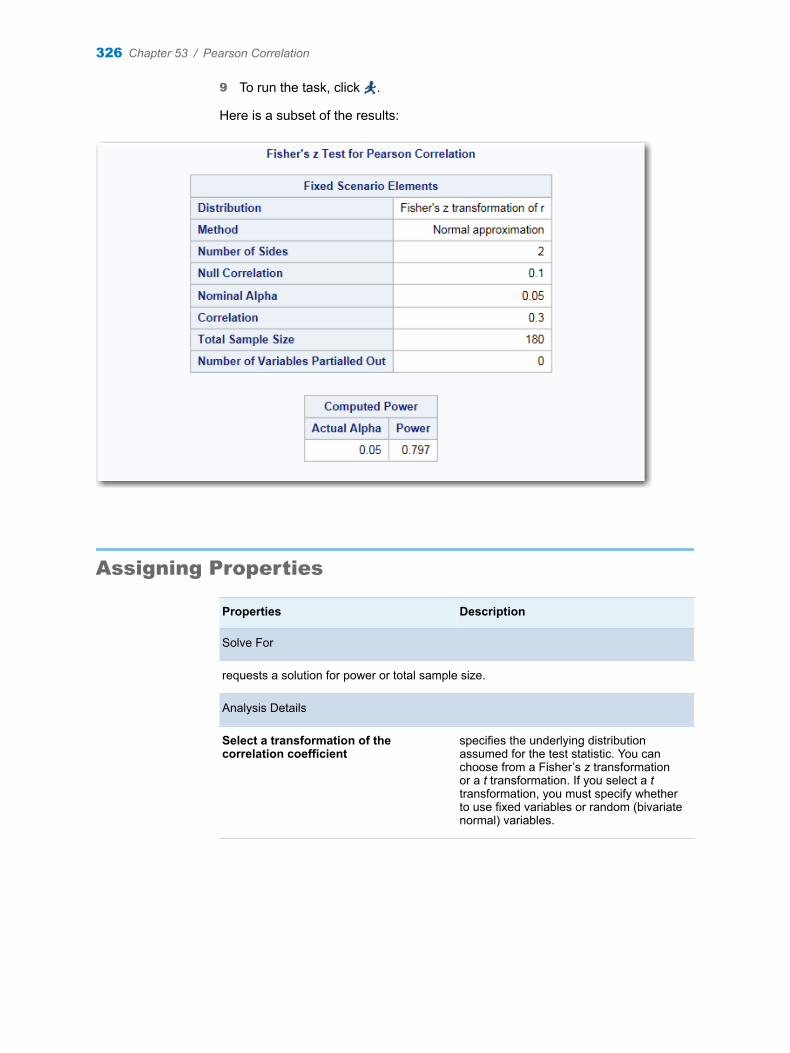
9 To run the task, click .
Here is a subset of the results:
Assigning Properties
Properties Description
Solve For
requests a solution for power or total sample size.
Analysis Details
Select a transformation of the correlation coefficient
specifies the underlying distribution assumed for the test statistic. You can choose from a Fisher’s z transformation or a t transformation. If you select a t transformation, you must specify whether to use fixed variables or random (bivariate normal) variables.
326 Chapter 53 / Pearson Correlation
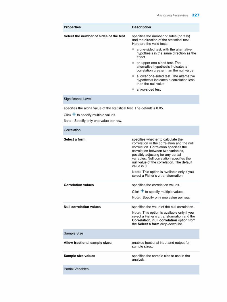
Properties Description
Select the number of sides of the test specifies the number of sides (or tails) and the direction of the statistical test. Here are the valid tests:n a one-sided test, with the alternative
hypothesis in the same direction as the effect.
n an upper one-sided test. The alternative hypothesis indicates a correlation greater than the null value.
n a lower one-sided test. The alternative hypothesis indicates a correlation less than the null value.
n a two-sided test
Significance Level
specifies the alpha value of the statistical test. The default is 0.05.
Click to specify multiple values.
Note: Specify only one value per row.
Correlation
Select a form specifies whether to calculate the correlation or the correlation and the null correlation. Correlation specifies the correlation between two variables, possibly adjusting for any partial variables. Null correlation specifies the null value of the correlation. The default value is 0.
Note: This option is available only if you select a Fisher’s z transformation.
Correlation values specifies the correlation values.
Click to specify multiple values.
Note: Specify only one value per row.
Null correlation values specifies the value of the null correlation.
Note: This option is available only if you select a Fisher’s z transformation and the Correlation, null correlation option from the Select a form drop-down list.
Sample Size
Allow fractional sample sizes enables fractional input and output for sample sizes.
Sample size values specifies the sample size to use in the analysis.
Partial Variables
Assigning Properties 327

Properties Description
Specify the number of variables to partial out
specifies the number of variables adjusted for the correlation between the two primary variables. The default value is 0, which corresponds to a simple correlation.
Setting the Plot Options
Option Name Description
Plots
Power by sample size plot creates a plot with sample size on the vertical axis and power on the horizontal axis.
For this plot, you can specify the minimum and maximum value for power.
Power (or sample size) by effect size plot
specifies a plot effect size on the horizontal axis. Power or sample size is on the vertical axis.
For this plot, you can specify the minimum and maximum value for the effect size.
328 Chapter 53 / Pearson Correlation
54Multiple Regression
About the Multiple Regression Task . . . . . . . . . . . . . . . . . . . . . . . . . . . . . . . . . . . . . . . 329
Example: Solve for Power . . . . . . . . . . . . . . . . . . . . . . . . . . . . . . . . . . . . . . . . . . . . . . . . . 329
Assigning Properties . . . . . . . . . . . . . . . . . . . . . . . . . . . . . . . . . . . . . . . . . . . . . . . . . . . . . . 331
Setting the Plot Options . . . . . . . . . . . . . . . . . . . . . . . . . . . . . . . . . . . . . . . . . . . . . . . . . . . 331
About the Multiple Regression Task
The Multiple Regression task calculates the power or sample size for multiple regression.
Example: Solve for Power
To create this example:
1 In the Tasks section, expand the Power and Sample Size folder, and then double-click Multiple Regression. The user interface for the Multiple Regression task opens.
2 Under the Solve For heading, select Power.
3 Under the Analysis Details heading, select Random predictors.
4 In the Number of full model predictors field, enter 7.
5 In the Number of reduced model predictors field, enter 3.
6 Under the Variance Accounted For heading, select Partial correlation from the Select a form drop-down list.
7 Enter .3 as the partial correlation.
8 For the sample size, enter 100.
To add a second sample size, click . In the second row, enter 50.
9 To run the task, click .
329

Here are the results:
330 Chapter 54 / Multiple Regression
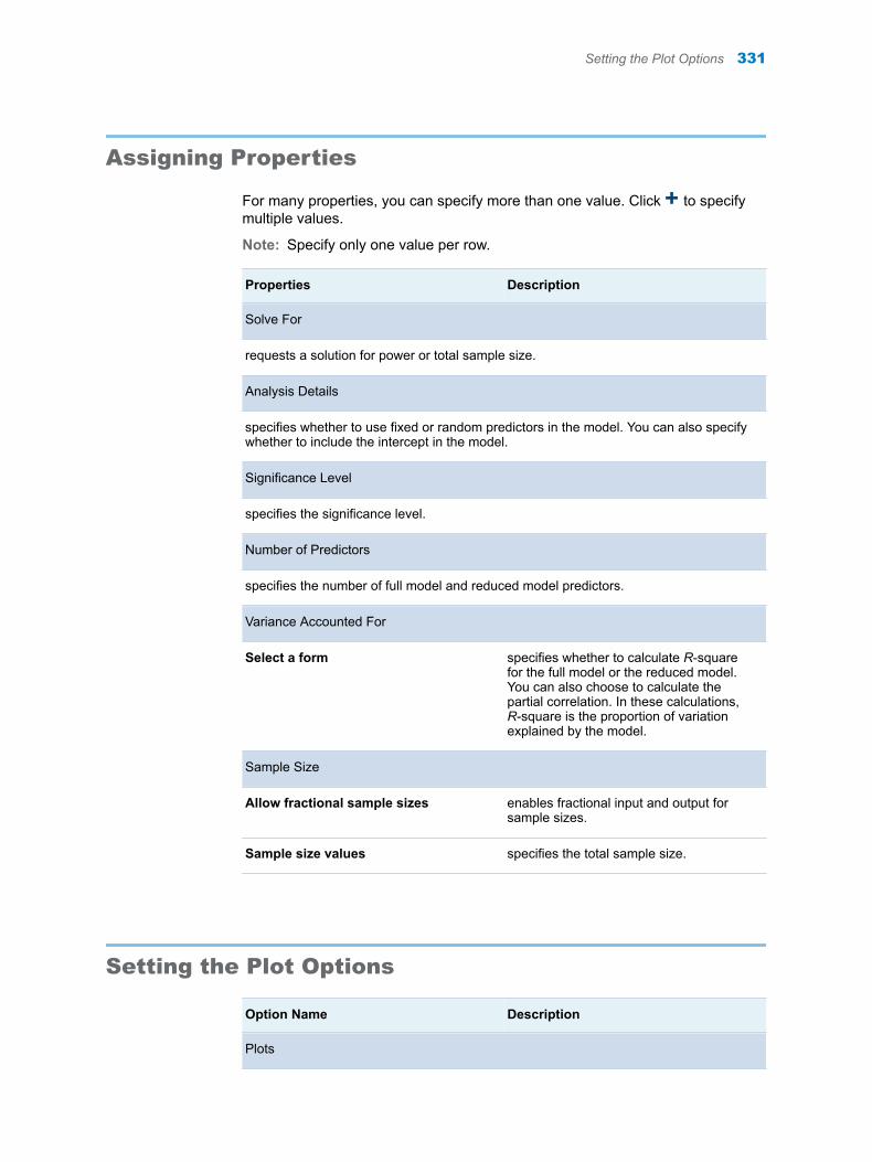
Assigning Properties
For many properties, you can specify more than one value. Click to specify multiple values.
Note: Specify only one value per row.
Properties Description
Solve For
requests a solution for power or total sample size.
Analysis Details
specifies whether to use fixed or random predictors in the model. You can also specify whether to include the intercept in the model.
Significance Level
specifies the significance level.
Number of Predictors
specifies the number of full model and reduced model predictors.
Variance Accounted For
Select a form specifies whether to calculate R-square for the full model or the reduced model. You can also choose to calculate the partial correlation. In these calculations, R-square is the proportion of variation explained by the model.
Sample Size
Allow fractional sample sizes enables fractional input and output for sample sizes.
Sample size values specifies the total sample size.
Setting the Plot Options
Option Name Description
Plots
Setting the Plot Options 331
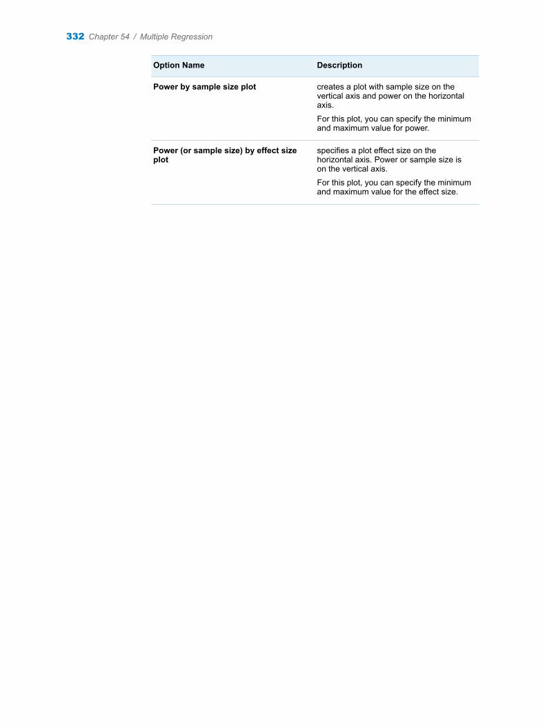
Option Name Description
Power by sample size plot creates a plot with sample size on the vertical axis and power on the horizontal axis.
For this plot, you can specify the minimum and maximum value for power.
Power (or sample size) by effect size plot
specifies a plot effect size on the horizontal axis. Power or sample size is on the vertical axis.
For this plot, you can specify the minimum and maximum value for the effect size.
332 Chapter 54 / Multiple Regression
55Confidence Intervals
About the Confidence Intervals Task . . . . . . . . . . . . . . . . . . . . . . . . . . . . . . . . . . . . . . 333
Example: Confidence Interval for One-Sample Means . . . . . . . . . . . . . . . . . . . . . . 333
Assigning Properties . . . . . . . . . . . . . . . . . . . . . . . . . . . . . . . . . . . . . . . . . . . . . . . . . . . . . . 334
Setting the Plot Options . . . . . . . . . . . . . . . . . . . . . . . . . . . . . . . . . . . . . . . . . . . . . . . . . . . 336
About the Confidence Intervals Task
The Confidence Intervals task calculates the power or sample size for these confidence intervals:
n One-sample means is for confidence interval precision involving one sample.
n Paired means is for confidence interval precision involving paired samples.
n Two-sample means is for confidence interval precision involving two independent samples.
n One proportion is for confidence interval precision for a single binomial proportion.
Example: Confidence Interval for One-Sample Means
To create this example:
1 In the Tasks section, expand the Power and Sample Size folder, and then double-click Confidence Intervals. The user interface for the Confidence Intervals task opens.
2 From the Type of confidence interval drop-down list, select One-sample mean.
3 Under the Solve For heading, select Prob(Width).
4 For the half width, enter 14.
5 For the standard deviation, enter 8.
333
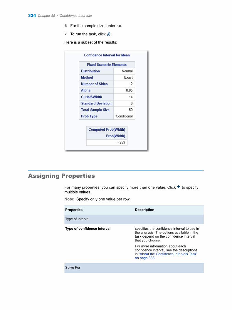
6 For the sample size, enter 50.
7 To run the task, click .
Here is a subset of the results:
Assigning Properties
For many properties, you can specify more than one value. Click to specify multiple values.
Note: Specify only one value per row.
Properties Description
Type of Interval
Type of confidence interval specifies the confidence interval to use in the analysis. The options available in the task depend on the confidence interval that you choose.
For more information about each confidence interval, see the descriptions in “About the Confidence Intervals Task” on page 333.
Solve For
334 Chapter 55 / Confidence Intervals
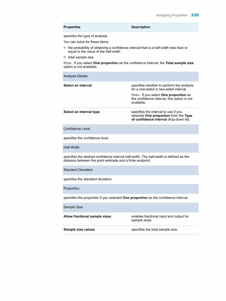
Properties Description
specifies the type of analysis.
You can solve for these items:
n the probability of obtaining a confidence interval that is a half-width less than or equal to the value of the half-width
n total sample size
Note: If you select One proportion as the confidence interval, the Total sample size option is not available.
Analysis Details
Select an interval specifies whether to perform the analysis for a one-sided or two-sided interval.
Note: If you select One proportion as the confidence interval, this option is not available.
Select an interval type specifies the interval to use if you selected One proportion from the Type of confidence interval drop-down list.
Confidence Level
specifies the confidence level.
Half-Width
specifies the desired confidence interval half-width. The half-width is defined as the distance between the point estimate and a finite endpoint.
Standard Deviation
specifies the standard deviation.
Proportion
specifies the proportion if you selected One proportion as the confidence interval.
Sample Size
Allow fractional sample sizes enables fractional input and output for sample sizes.
Sample size values specifies the total sample size.
Assigning Properties 335
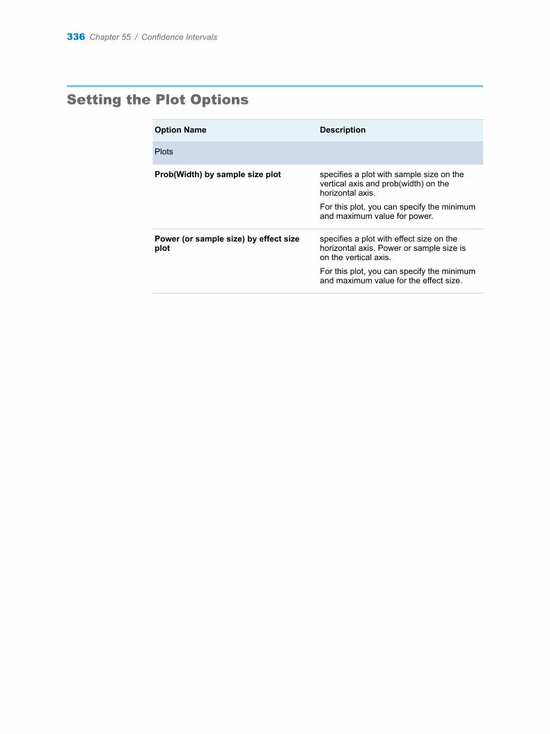
Setting the Plot Options
Option Name Description
Plots
Prob(Width) by sample size plot specifies a plot with sample size on the vertical axis and prob(width) on the horizontal axis.
For this plot, you can specify the minimum and maximum value for power.
Power (or sample size) by effect size plot
specifies a plot with effect size on the horizontal axis. Power or sample size is on the vertical axis.
For this plot, you can specify the minimum and maximum value for the effect size.
336 Chapter 55 / Confidence Intervals
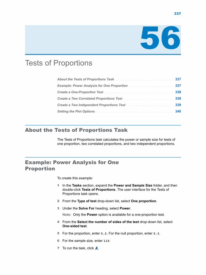
56Tests of Proportions
About the Tests of Proportions Task . . . . . . . . . . . . . . . . . . . . . . . . . . . . . . . . . . . . . . . 337
Example: Power Analysis for One Proportion . . . . . . . . . . . . . . . . . . . . . . . . . . . . . . 337
Create a One-Proportion Test . . . . . . . . . . . . . . . . . . . . . . . . . . . . . . . . . . . . . . . . . . . . . . 338
Create a Two Correlated Proportions Test . . . . . . . . . . . . . . . . . . . . . . . . . . . . . . . . . 339
Create a Two Independent Proportions Test . . . . . . . . . . . . . . . . . . . . . . . . . . . . . . . 339
Setting the Plot Options . . . . . . . . . . . . . . . . . . . . . . . . . . . . . . . . . . . . . . . . . . . . . . . . . . . 340
About the Tests of Proportions Task
The Tests of Proportions task calculates the power or sample size for tests of one proportion, two correlated proportions, and two independent proportions.
Example: Power Analysis for One Proportion
To create this example:
1 In the Tasks section, expand the Power and Sample Size folder, and then double-click Tests of Proportions. The user interface for the Tests of Proportions task opens.
2 From the Type of test drop-down list, select One proportion.
3 Under the Solve For heading, select Power.
Note: Only the Power option is available for a one-proportion test.
4 From the Select the number of sides of the test drop-down list, select One-sided test.
5 For the proportion, enter 0.2. For the null proportion, enter 0.3.
6 For the sample size, enter 119.
7 To run the task, click .
337

Here is a subset of the results:
Create a One-Proportion Test
To create a one-proportion test:
1 From the Type of test drop-down list, select One proportion.
2 For the quantity to solve for, select Power.
Note: To solve for a total sample size, you must select Approximate Z-test or Approximate continuity-adjusted Z-test from the Select a test drop-down list.
3 Select the test to perform. You can choose from these options:
n Exact binomial test
n Exact Z-test
n Exact continuity-adjusted Z-test
n Approximate Z-test
n Approximate continuity-adjusted Z-test
4 Select the variance estimate for the test. The variance can be based on either the null proportion or the observed sample proportion.
Note: This option is not available if you are performing an exact binomial test.
5 Select whether to perform a one-sided test or a two-sided test.
6 Specify the significance level.
7 Specify the proportion and the null proportion.
338 Chapter 56 / Tests of Proportions

8 Specify the sample size and whether to allow for fractional sample sizes.
Create a Two Correlated Proportions Test
To create a two correlated proportions test:
1 From the Type of test drop-down list, select Two correlated proportions.
2 Under the Solve For heading, select Power or Total sample size.
3 Select the method to use:
n Exact
n Connor approximation
n Miettinen approximation
4 Select the distribution for the test statistic:
n Exact conditional
n Normal approximation to the binomial
5 Select whether to perform a one-sided test or a two-sided test.
6 Specify the significance level.
7 Specify the values for proportions, odds ratios, or relative risk.
8 Specify whether to allow for fractional sample sizes and the number of pairs.
Create a Two Independent Proportions Test
To create a two independent proportions test:
1 From the Type of test drop-down list, select Two independent proportions.
2 For the quantity to solve for, select Power or Sample size per group.
3 Select the test to use:
n Fisher’s exact test
n Farrington-Manning score test
n Likelihood ratio chi-square test
n Pearson chi-square test
4 Select whether to perform a one-sided test or a two-sided test.
5 Specify the significance level.
6 Specify the form of the proportion and any related values.
Create a Two Independent Proportions Test 339

7 Specify whether to allow for fractional sample sizes and the form of the sample size.
Setting the Plot Options
Option Name Description
Plots
Power by sample size plot creates a plot with sample size on the vertical axis and power on the horizontal axis.
For this plot, you can specify the minimum and maximum value for power.
Power (or sample size) by effect size plot
specifies a plot effect size on the horizontal axis. Power or sample size is on the vertical axis.
For this plot, you can specify the minimum and maximum value for the effect size.
340 Chapter 56 / Tests of Proportions
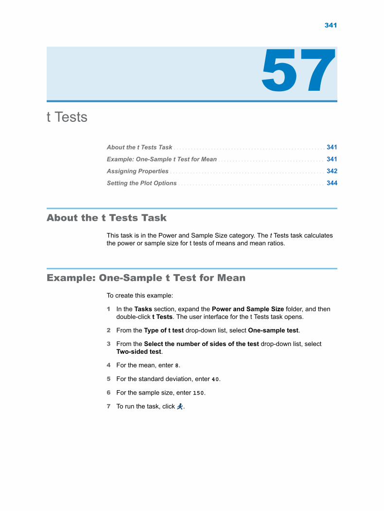
57t Tests
About the t Tests Task . . . . . . . . . . . . . . . . . . . . . . . . . . . . . . . . . . . . . . . . . . . . . . . . . . . . . 341
Example: One-Sample t Test for Mean . . . . . . . . . . . . . . . . . . . . . . . . . . . . . . . . . . . . . 341
Assigning Properties . . . . . . . . . . . . . . . . . . . . . . . . . . . . . . . . . . . . . . . . . . . . . . . . . . . . . . 342
Setting the Plot Options . . . . . . . . . . . . . . . . . . . . . . . . . . . . . . . . . . . . . . . . . . . . . . . . . . . 344
About the t Tests Task
This task is in the Power and Sample Size category. The t Tests task calculates the power or sample size for t tests of means and mean ratios.
Example: One-Sample t Test for Mean
To create this example:
1 In the Tasks section, expand the Power and Sample Size folder, and then double-click t Tests. The user interface for the t Tests task opens.
2 From the Type of t test drop-down list, select One-sample test.
3 From the Select the number of sides of the test drop-down list, select Two-sided test.
4 For the mean, enter 8.
5 For the standard deviation, enter 40.
6 For the sample size, enter 150.
7 To run the task, click .
341
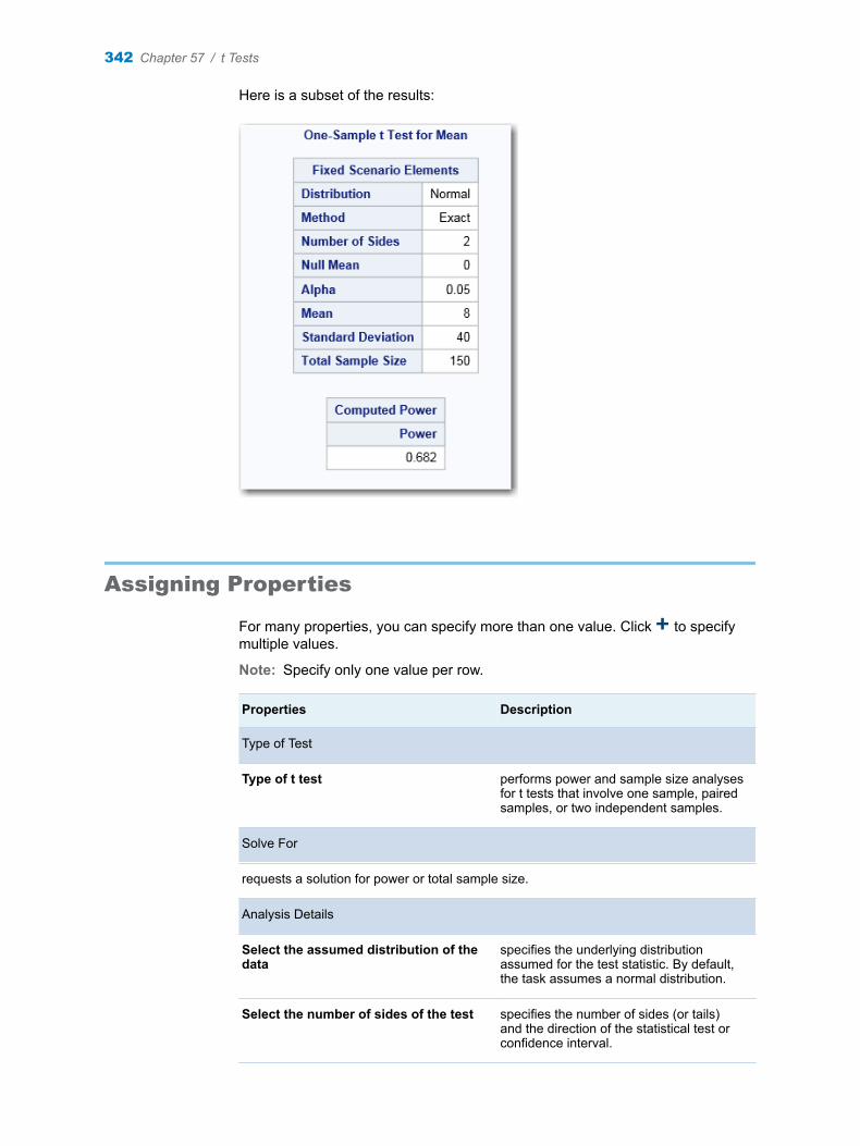
Here is a subset of the results:
Assigning Properties
For many properties, you can specify more than one value. Click to specify multiple values.
Note: Specify only one value per row.
Properties Description
Type of Test
Type of t test performs power and sample size analyses for t tests that involve one sample, paired samples, or two independent samples.
Solve For
requests a solution for power or total sample size.
Analysis Details
Select the assumed distribution of the data
specifies the underlying distribution assumed for the test statistic. By default, the task assumes a normal distribution.
Select the number of sides of the test specifies the number of sides (or tails) and the direction of the statistical test or confidence interval.
342 Chapter 57 / t Tests
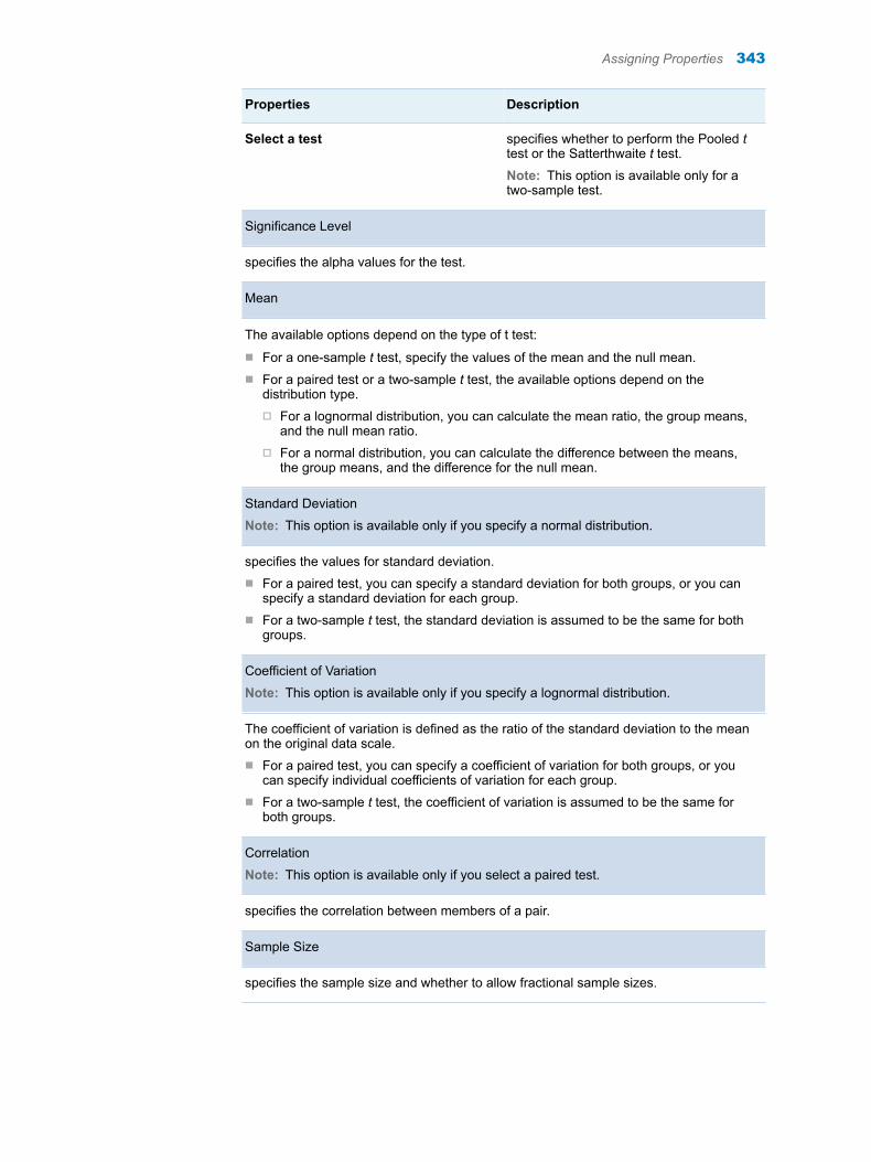
Properties Description
Select a test specifies whether to perform the Pooled t test or the Satterthwaite t test.
Note: This option is available only for a two-sample test.
Significance Level
specifies the alpha values for the test.
Mean
The available options depend on the type of t test:
n For a one-sample t test, specify the values of the mean and the null mean. n For a paired test or a two-sample t test, the available options depend on the
distribution type.o For a lognormal distribution, you can calculate the mean ratio, the group means,
and the null mean ratio.o For a normal distribution, you can calculate the difference between the means,
the group means, and the difference for the null mean.
Standard Deviation
Note: This option is available only if you specify a normal distribution.
specifies the values for standard deviation.n For a paired test, you can specify a standard deviation for both groups, or you can
specify a standard deviation for each group. n For a two-sample t test, the standard deviation is assumed to be the same for both
groups.
Coefficient of Variation
Note: This option is available only if you specify a lognormal distribution.
The coefficient of variation is defined as the ratio of the standard deviation to the mean on the original data scale.n For a paired test, you can specify a coefficient of variation for both groups, or you
can specify individual coefficients of variation for each group.n For a two-sample t test, the coefficient of variation is assumed to be the same for
both groups.
Correlation
Note: This option is available only if you select a paired test.
specifies the correlation between members of a pair.
Sample Size
specifies the sample size and whether to allow fractional sample sizes.
Assigning Properties 343
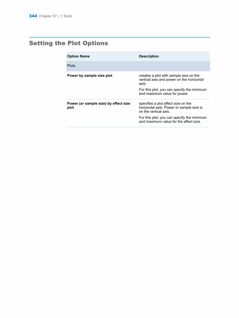
Setting the Plot Options
Option Name Description
Plots
Power by sample size plot creates a plot with sample size on the vertical axis and power on the horizontal axis.
For this plot, you can specify the minimum and maximum value for power.
Power (or sample size) by effect size plot
specifies a plot effect size on the horizontal axis. Power or sample size is on the vertical axis.
For this plot, you can specify the minimum and maximum value for the effect size.
344 Chapter 57 / t Tests
58Cox Regression
About the Cox Regression Task . . . . . . . . . . . . . . . . . . . . . . . . . . . . . . . . . . . . . . . . . . . 345
Example: Cox Regression . . . . . . . . . . . . . . . . . . . . . . . . . . . . . . . . . . . . . . . . . . . . . . . . . 345
Assigning Properties . . . . . . . . . . . . . . . . . . . . . . . . . . . . . . . . . . . . . . . . . . . . . . . . . . . . . . 346
Setting the Plot Options . . . . . . . . . . . . . . . . . . . . . . . . . . . . . . . . . . . . . . . . . . . . . . . . . . . 347
About the Cox Regression Task
The Cox Regression task calculates the power or sample size for the score test. This test is for a single scalar predictor in Cox proportional hazards regression for survival data.
Example: Cox Regression
To create this example:
1 In the Tasks section, expand the Power and Sample Size folder, and then double-click Cox Regression. The user interface for the Cox Regression task opens.
2 Under the Solve For heading, select Power.
3 For the hazard ratio, enter 1.4.
4 For the R-square value, enter .15.
5 For the standard deviation, enter 1.2.
6 For the probabilities of uncensored events, enter 0.8.
7 For the sample size, enter 80.
8 To run the task, click .
345

Here is a subset of the results:
Assigning Properties
For many properties, you can specify more than one value. Click to specify multiple values.
Note: Specify only one value per row.
Properties Description
Solve For
Select the quantity to solve for requests a solution for power, total sample size, or total number of uncensored events.
Analysis Details
Select the number of sides of the test specifies whether to perform a one-sided test or two-sided test.
Significance Level
specifies the alpha values.
Hazard Ratio
346 Chapter 58 / Cox Regression
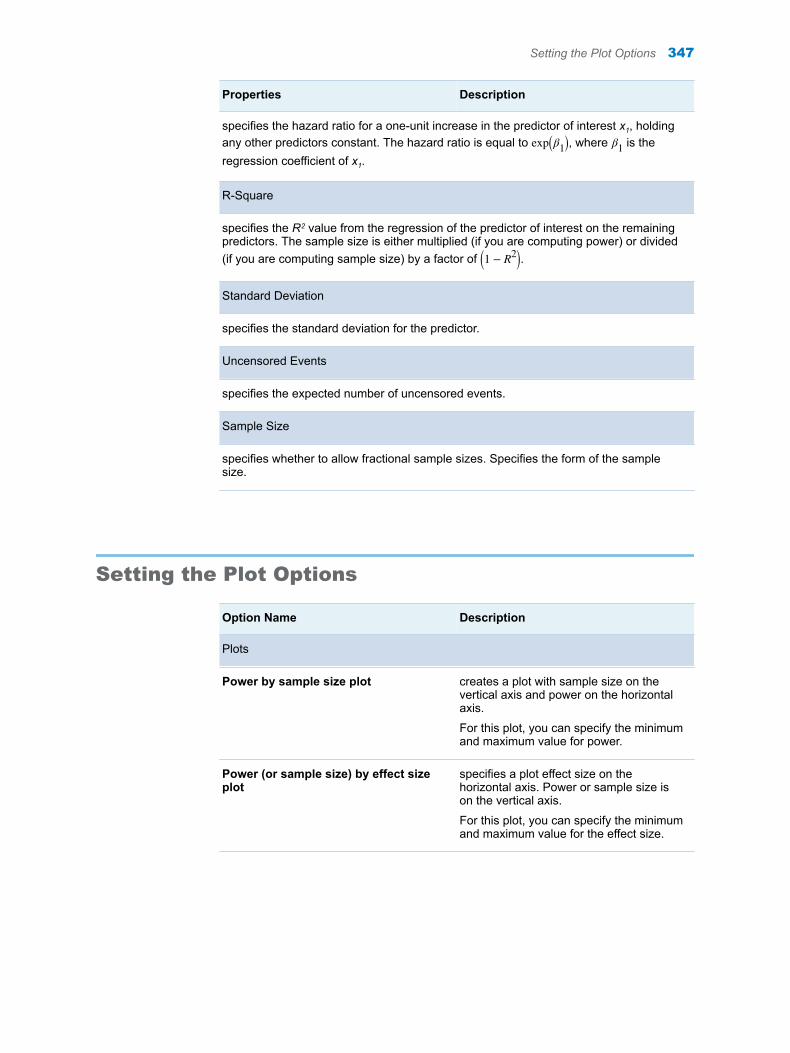
Properties Description
specifies the hazard ratio for a one-unit increase in the predictor of interest x1, holding any other predictors constant. The hazard ratio is equal to exp β1 , where β1 is the regression coefficient of x1.
R-Square
specifies the R2 value from the regression of the predictor of interest on the remaining predictors. The sample size is either multiplied (if you are computing power) or divided (if you are computing sample size) by a factor of 1 − R2 .
Standard Deviation
specifies the standard deviation for the predictor.
Uncensored Events
specifies the expected number of uncensored events.
Sample Size
specifies whether to allow fractional sample sizes. Specifies the form of the sample size.
Setting the Plot Options
Option Name Description
Plots
Power by sample size plot creates a plot with sample size on the vertical axis and power on the horizontal axis.
For this plot, you can specify the minimum and maximum value for power.
Power (or sample size) by effect size plot
specifies a plot effect size on the horizontal axis. Power or sample size is on the vertical axis.
For this plot, you can specify the minimum and maximum value for the effect size.
Setting the Plot Options 347

348 Chapter 58 / Cox Regression
Part 7
Multivariate Analysis
Chapter 59Principal Component Analysis . . . . . . . . . . . . . . . . . . . . . . . . . . . . . . . . . . . . 351
Chapter 60Factor Analysis . . . . . . . . . . . . . . . . . . . . . . . . . . . . . . . . . . . . . . . . . . . . . . . . . 355
Chapter 61Canonical Correlation . . . . . . . . . . . . . . . . . . . . . . . . . . . . . . . . . . . . . . . . . . . . 363
Chapter 62Discriminant Analysis . . . . . . . . . . . . . . . . . . . . . . . . . . . . . . . . . . . . . . . . . . . . 369
Chapter 63Correspondence Analysis . . . . . . . . . . . . . . . . . . . . . . . . . . . . . . . . . . . . . . . . 377
Chapter 64Multidimensional Preferences Analysis . . . . . . . . . . . . . . . . . . . . . . . . . . . . 385
349

350
59Principal Component Analysis
About the Principal Component Analysis Task . . . . . . . . . . . . . . . . . . . . . . . . . . . . . 351
Example: Principal Component Analysis of Sashelp.Class Data Set . . . . . . . . 351
Assigning Data to Roles . . . . . . . . . . . . . . . . . . . . . . . . . . . . . . . . . . . . . . . . . . . . . . . . . . . 353
Setting Options . . . . . . . . . . . . . . . . . . . . . . . . . . . . . . . . . . . . . . . . . . . . . . . . . . . . . . . . . . . . 353
Setting the Output Options . . . . . . . . . . . . . . . . . . . . . . . . . . . . . . . . . . . . . . . . . . . . . . . . 354
About the Principal Component Analysis Task
Principal component analysis is a multivariate technique for examining relationships among several quantitative variables. Use principal component analysis if you are interested in summarizing data and detecting linear relationships.
Example: Principal Component Analysis of Sashelp.Class Data Set
To create this example:
1 In the Tasks section, expand the Multivariate Analysis folder, and then double-click Principal Component Analysis. The user interface for the Principal Component Analysis task opens.
2 On the Data tab, select the SASHELP.CLASS data set.
TIP If the data set is not available from the drop-down list, click . In
the Choose a Table window, expand the library that contains the data set that you want to use. Select the data set for the example and click OK. The selected data set should now appear in the drop-down list.
3 Assign columns to these roles:
351
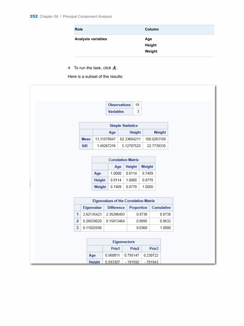
Role Column
Analysis variables AgeHeightWeight
4 To run the task, click .
Here is a subset of the results:
352 Chapter 59 / Principal Component Analysis
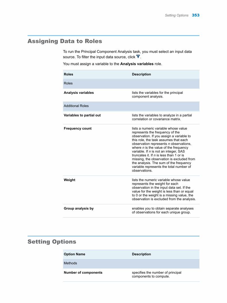
Assigning Data to Roles
To run the Principal Component Analysis task, you must select an input data source. To filter the input data source, click .
You must assign a variable to the Analysis variables role.
Roles Description
Roles
Analysis variables lists the variables for the principal component analysis.
Additional Roles
Variables to partial out lists the variables to analyze in a partial correlation or covariance matrix.
Frequency count lists a numeric variable whose value represents the frequency of the observation. If you assign a variable to this role, the task assumes that each observation represents n observations, where n is the value of the frequency variable. If n is not an integer, SAS truncates it. If n is less than 1 or is missing, the observation is excluded from the analysis. The sum of the frequency variable represents the total number of observations.
Weight lists the numeric variable whose value represents the weight for each observation in the input data set. If the value for the weight is less than or equal to 0 or the weight is a missing value, the observation is excluded from the analysis.
Group analysis by enables you to obtain separate analyses of observations for each unique group.
Setting Options
Option Name Description
Methods
Number of components specifies the number of principal components to compute.
Setting Options 353
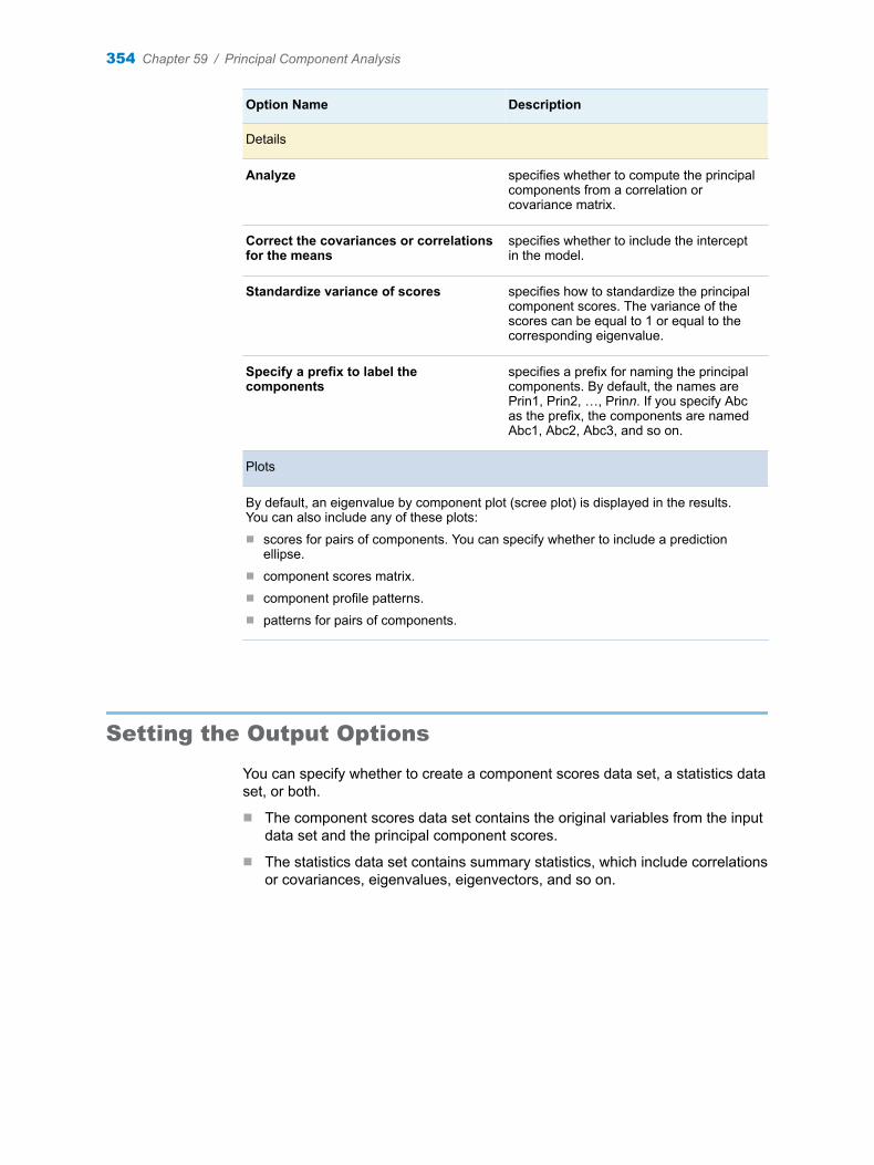
Option Name Description
Details
Analyze specifies whether to compute the principal components from a correlation or covariance matrix.
Correct the covariances or correlations for the means
specifies whether to include the intercept in the model.
Standardize variance of scores specifies how to standardize the principal component scores. The variance of the scores can be equal to 1 or equal to the corresponding eigenvalue.
Specify a prefix to label the components
specifies a prefix for naming the principal components. By default, the names are Prin1, Prin2, …, Prinn. If you specify Abc as the prefix, the components are named Abc1, Abc2, Abc3, and so on.
Plots
By default, an eigenvalue by component plot (scree plot) is displayed in the results. You can also include any of these plots:n scores for pairs of components. You can specify whether to include a prediction
ellipse.n component scores matrix.n component profile patterns.n patterns for pairs of components.
Setting the Output Options
You can specify whether to create a component scores data set, a statistics data set, or both.
n The component scores data set contains the original variables from the input data set and the principal component scores.
n The statistics data set contains summary statistics, which include correlations or covariances, eigenvalues, eigenvectors, and so on.
354 Chapter 59 / Principal Component Analysis

60Factor Analysis
About the Factor Analysis Task . . . . . . . . . . . . . . . . . . . . . . . . . . . . . . . . . . . . . . . . . . . . 355
Example: Factor Analysis . . . . . . . . . . . . . . . . . . . . . . . . . . . . . . . . . . . . . . . . . . . . . . . . . 355
Assigning Data to Roles . . . . . . . . . . . . . . . . . . . . . . . . . . . . . . . . . . . . . . . . . . . . . . . . . . . 357
Setting Options . . . . . . . . . . . . . . . . . . . . . . . . . . . . . . . . . . . . . . . . . . . . . . . . . . . . . . . . . . . . 358
Setting the Output Options . . . . . . . . . . . . . . . . . . . . . . . . . . . . . . . . . . . . . . . . . . . . . . . . 361
About the Factor Analysis Task
The Factor Analysis task performs a factor analysis with a variety of available methods and rotations.
Example: Factor Analysis
To create this example:
1 In the Tasks section, expand the Multivariate Analysis folder, and then double-click Factor Analysis. The user interface for the Factor Analysis task opens.
2 On the Data tab, select the SASHELP.BASEBALL data set.
TIP If the data set is not available from the drop-down list, click . In
the Choose a Table window, expand the library that contains the data set that you want to use. Select the data set for the example and click OK. The selected data set should now appear in the drop-down list.
3 Assign columns to these roles:
355

Role Column
Analysis variables nAtBatnHitsnHomenRunsnRBInBBYrMajorCrAtBat
4 On the Options tab, select these options:
n From the Rotation method drop-down list, select Varimax.
n For the type of rotation, select Orthogonal rotation.
5 To run the task, click .
Here is a subset of the results:
356 Chapter 60 / Factor Analysis
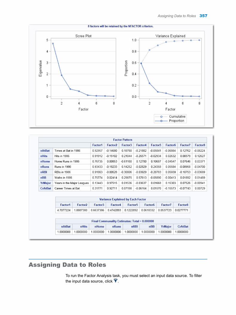
Assigning Data to Roles
To run the Factor Analysis task, you must select an input data source. To filter the input data source, click .
Assigning Data to Roles 357
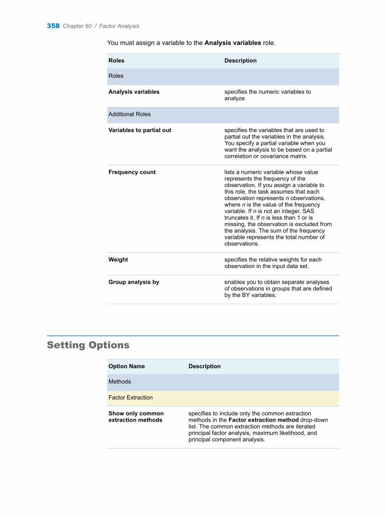
You must assign a variable to the Analysis variables role.
Roles Description
Roles
Analysis variables specifies the numeric variables to analyze.
Additional Roles
Variables to partial out specifies the variables that are used to partial out the variables in the analysis. You specify a partial variable when you want the analysis to be based on a partial correlation or covariance matrix.
Frequency count lists a numeric variable whose value represents the frequency of the observation. If you assign a variable to this role, the task assumes that each observation represents n observations, where n is the value of the frequency variable. If n is not an integer, SAS truncates it. If n is less than 1 or is missing, the observation is excluded from the analysis. The sum of the frequency variable represents the total number of observations.
Weight specifies the relative weights for each observation in the input data set.
Group analysis by enables you to obtain separate analyses of observations in groups that are defined by the BY variables.
Setting Options
Option Name Description
Methods
Factor Extraction
Show only common extraction methods
specifies to include only the common extraction methods in the Factor extraction method drop-down list. The common extraction methods are iterated principal factor analysis, maximum likelihood, and principal component analysis.
358 Chapter 60 / Factor Analysis
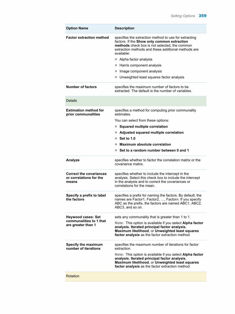
Option Name Description
Factor extraction method specifies the extraction method to use for extracting factors. If the Show only common extraction methods check box is not selected, the common extraction methods and these additional methods are available:n Alpha factor analysisn Harris component analysisn Image component analysisn Unweighted least squares factor analysis
Number of factors specifies the maximum number of factors to be extracted. The default is the number of variables.
Details
Estimation method for prior communalities
specifies a method for computing prior communality estimates.
You can select from these options:
n Squared multiple correlationn Adjusted squared multiple correlationn Set to 1.0n Maximum absolute correlationn Set to a random number between 0 and 1
Analyze specifies whether to factor the correlation matrix or the covariance matrix.
Correct the covariances or correlations for the means
specifies whether to include the intercept in the analysis. Select this check box to include the intercept in the analysis and to correct the covariances or correlations for the mean.
Specify a prefix to label the factors
specifies a prefix for naming the factors. By default, the names are Factor1, Factor2, …, Factorn. If you specify ABC as the prefix, the factors are named ABC1, ABC2, ABC3, and so on.
Heywood cases: Set communalities to 1 that are greater than 1
sets any communality that is greater than 1 to 1.
Note: This option is available if you select Alpha factor analysis, Iterated principal factor analysis, Maximum likelihood, or Unweighted least squares factor analysis as the factor extraction method.
Specify the maximum number of iterations
specifies the maximum number of iterations for factor extraction.
Note: This option is available if you select Alpha factor analysis, Iterated principal factor analysis, Maximum likelihood, or Unweighted least squares factor analysis as the factor extraction method.
Rotation
Setting Options 359
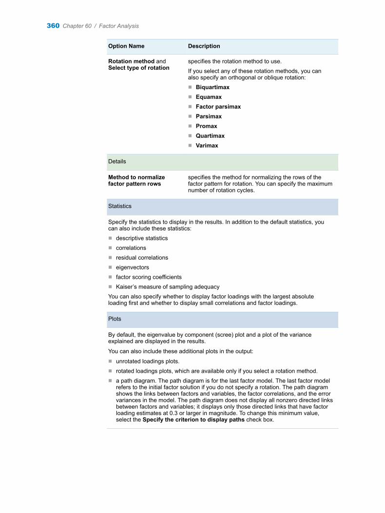
Option Name Description
Rotation method and Select type of rotation
specifies the rotation method to use.
If you select any of these rotation methods, you can also specify an orthogonal or oblique rotation:n Biquartimaxn Equamaxn Factor parsimaxn Parsimaxn Promaxn Quartimaxn Varimax
Details
Method to normalize factor pattern rows
specifies the method for normalizing the rows of the factor pattern for rotation. You can specify the maximum number of rotation cycles.
Statistics
Specify the statistics to display in the results. In addition to the default statistics, you can also include these statistics:n descriptive statisticsn correlationsn residual correlationsn eigenvectorsn factor scoring coefficientsn Kaiser’s measure of sampling adequacy
You can also specify whether to display factor loadings with the largest absolute loading first and whether to display small correlations and factor loadings.
Plots
By default, the eigenvalue by component (scree) plot and a plot of the variance explained are displayed in the results.
You can also include these additional plots in the output:
n unrotated loadings plots.n rotated loadings plots, which are available only if you select a rotation method.n a path diagram. The path diagram is for the last factor model. The last factor model
refers to the initial factor solution if you do not specify a rotation. The path diagram shows the links between factors and variables, the factor correlations, and the error variances in the model. The path diagram does not display all nonzero directed links between factors and variables; it displays only those directed links that have factor loading estimates at 0.3 or larger in magnitude. To change this minimum value, select the Specify the criterion to display paths check box.
360 Chapter 60 / Factor Analysis

Setting the Output Options
You can specify whether to create a factor scores data set, a statistics data set, or both.
Setting the Output Options 361

362 Chapter 60 / Factor Analysis
61Canonical Correlation
About the Canonical Correlation Analysis Task . . . . . . . . . . . . . . . . . . . . . . . . . . . . 363
Example: Canonical Correlation Analysis . . . . . . . . . . . . . . . . . . . . . . . . . . . . . . . . . . 363
Assigning Data to Roles . . . . . . . . . . . . . . . . . . . . . . . . . . . . . . . . . . . . . . . . . . . . . . . . . . . 365
Setting Options . . . . . . . . . . . . . . . . . . . . . . . . . . . . . . . . . . . . . . . . . . . . . . . . . . . . . . . . . . . . 366
Setting the Output Options . . . . . . . . . . . . . . . . . . . . . . . . . . . . . . . . . . . . . . . . . . . . . . . . 367
About the Canonical Correlation Analysis Task
Canonical correlation is a generalization of multiple correlations for analyzing the relationship between two sets of variables. The Canonical Correlation task performs canonical correlation, partial canonical correlation, and canonical redundancy analysis.
Example: Canonical Correlation Analysis
To create this example:
1 In SAS Studio, click and select New SAS Program.
2 Copy and paste this code into the Program tab.
data jobs; input career supervisor finance variety feedback autonomy; datalines;72 26 9 10 11 7063 76 7 85 22 9396 31 7 83 63 7396 98 6 82 75 9784 94 6 36 77 9766 10 5 28 24 7531 40 9 64 23 7545 14 2 19 15 5042 18 6 33 13 70
363
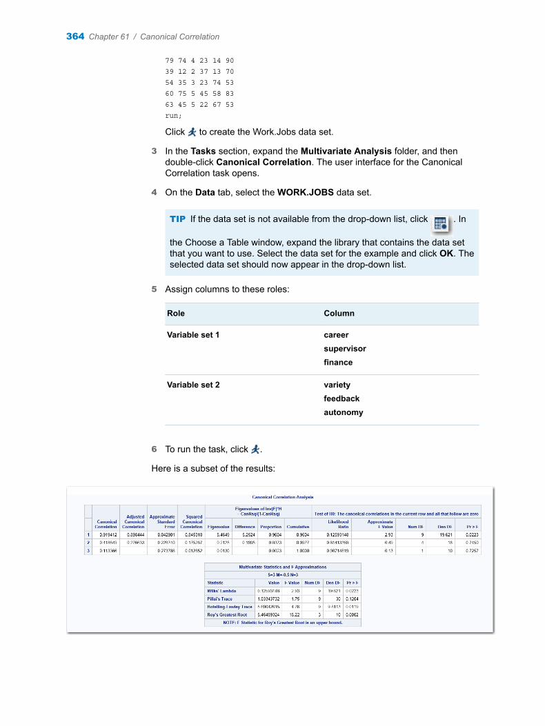
79 74 4 23 14 9039 12 2 37 13 7054 35 3 23 74 5360 75 5 45 58 8363 45 5 22 67 53run;
Click to create the Work.Jobs data set.
3 In the Tasks section, expand the Multivariate Analysis folder, and then double-click Canonical Correlation. The user interface for the Canonical Correlation task opens.
4 On the Data tab, select the WORK.JOBS data set.
TIP If the data set is not available from the drop-down list, click . In
the Choose a Table window, expand the library that contains the data set that you want to use. Select the data set for the example and click OK. The selected data set should now appear in the drop-down list.
5 Assign columns to these roles:
Role Column
Variable set 1 careersupervisorfinance
Variable set 2 varietyfeedbackautonomy
6 To run the task, click .
Here is a subset of the results:
364 Chapter 61 / Canonical Correlation
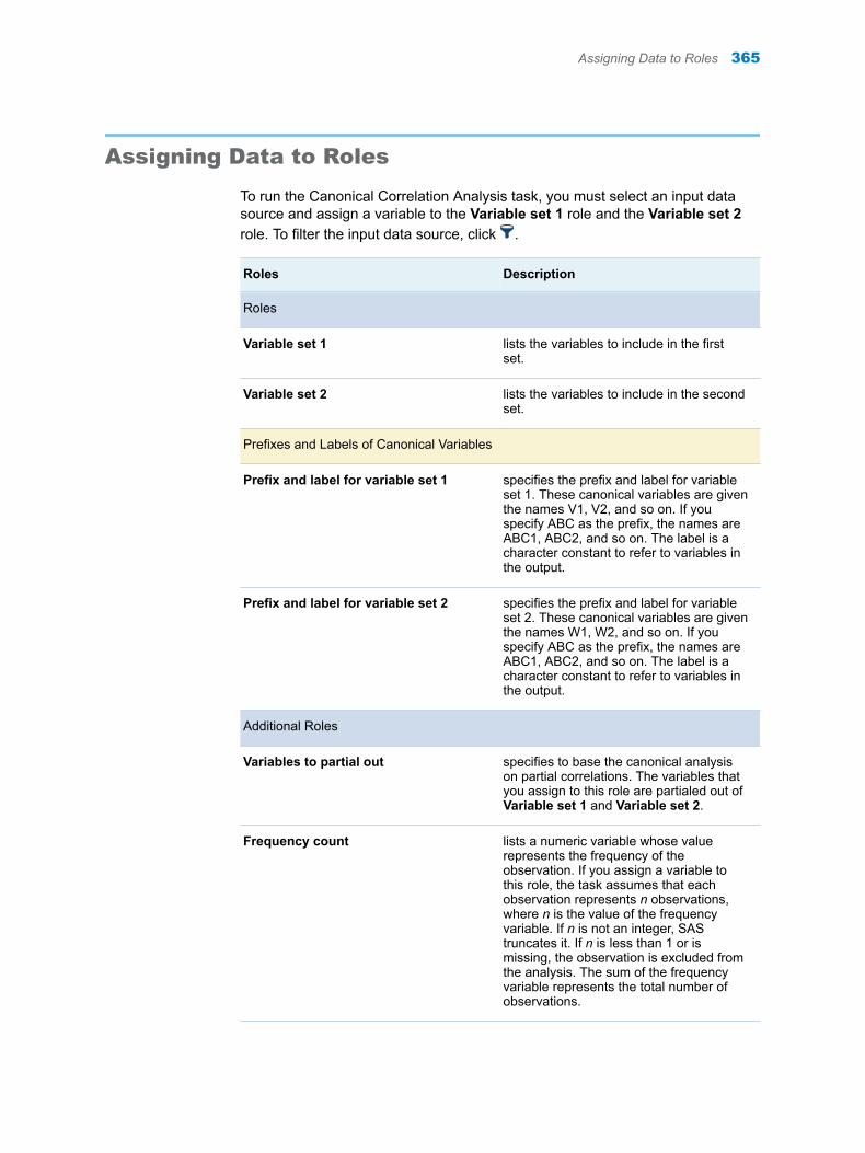
Assigning Data to Roles
To run the Canonical Correlation Analysis task, you must select an input data source and assign a variable to the Variable set 1 role and the Variable set 2 role. To filter the input data source, click .
Roles Description
Roles
Variable set 1 lists the variables to include in the first set.
Variable set 2 lists the variables to include in the second set.
Prefixes and Labels of Canonical Variables
Prefix and label for variable set 1 specifies the prefix and label for variable set 1. These canonical variables are given the names V1, V2, and so on. If you specify ABC as the prefix, the names are ABC1, ABC2, and so on. The label is a character constant to refer to variables in the output.
Prefix and label for variable set 2 specifies the prefix and label for variable set 2. These canonical variables are given the names W1, W2, and so on. If you specify ABC as the prefix, the names are ABC1, ABC2, and so on. The label is a character constant to refer to variables in the output.
Additional Roles
Variables to partial out specifies to base the canonical analysis on partial correlations. The variables that you assign to this role are partialed out of Variable set 1 and Variable set 2.
Frequency count lists a numeric variable whose value represents the frequency of the observation. If you assign a variable to this role, the task assumes that each observation represents n observations, where n is the value of the frequency variable. If n is not an integer, SAS truncates it. If n is less than 1 or is missing, the observation is excluded from the analysis. The sum of the frequency variable represents the total number of observations.
Assigning Data to Roles 365

Roles Description
Weight specifies the numeric variable to compute weighted product-moment correlation coefficients.
Group analysis by enables you to obtain separate analyses of observations for each unique group.
Setting Options
Option Name Description
Canonical Analysis
Canonical redundancy statistics produces canonical redundancy statistics.
Specify number of canonical variates specifies the number of canonical variables for which full output is desired. This number must be less than or equal to the number of canonical variables in the analysis.
Regression Analysis
Perform regression performs a regression analysis. You can select from these regression types:n Set 1 predicts Set 2 performs a
multiple regression analysis with variable set 1 as the regressors and variable set 2 as the dependent variables.
n Set 2 predicts Set 1 performs a multiple regression analysis with variable set 2 as the regressors and variable set 1 as the dependent variables.
Regression Statistics
You can include these regression statistics in the output:n regression coefficientsn standardized regression coefficientsn standardized error of coefficientsn t statistics for coefficientsn squared multiple correlation
Correlations
366 Chapter 61 / Canonical Correlation
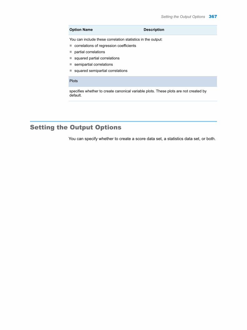
Option Name Description
You can include these correlation statistics in the output:n correlations of regression coefficientsn partial correlationsn squared partial correlationsn semipartial correlationsn squared semipartial correlations
Plots
specifies whether to create canonical variable plots. These plots are not created by default.
Setting the Output Options
You can specify whether to create a score data set, a statistics data set, or both.
Setting the Output Options 367

368 Chapter 61 / Canonical Correlation
62Discriminant Analysis
About the Discriminant Analysis Task . . . . . . . . . . . . . . . . . . . . . . . . . . . . . . . . . . . . . 369
Example: Discriminant Analysis on Crops Data . . . . . . . . . . . . . . . . . . . . . . . . . . . . 369
Assigning Data to Roles . . . . . . . . . . . . . . . . . . . . . . . . . . . . . . . . . . . . . . . . . . . . . . . . . . . 372
Setting Options . . . . . . . . . . . . . . . . . . . . . . . . . . . . . . . . . . . . . . . . . . . . . . . . . . . . . . . . . . . . 373
Setting the Selection Options . . . . . . . . . . . . . . . . . . . . . . . . . . . . . . . . . . . . . . . . . . . . . . 375
Setting the Output Options . . . . . . . . . . . . . . . . . . . . . . . . . . . . . . . . . . . . . . . . . . . . . . . . 376
About the Discriminant Analysis Task
For a set of observations with one or more quantitative variables and a classification variable, the Discriminant Analysis task develops a discriminant criterion to classify each observation into a group. The derived discriminant criterion from this data set can be applied to a second data set during the same run.
This task can also derive canonical variables. These variables are linear combinations of the quantitative variables that summarize between class variance. This summarization is similar to how principal components summarize total variation.
Example: Discriminant Analysis on Crops Data
To create this example:
1 In SAS Studio, click and select New SAS Program.
2 Create the Crops data set by copying and pasting this code into a Program tab.
data crops; length crop $ 10; input Crop x1-x4 ; datalines;
369
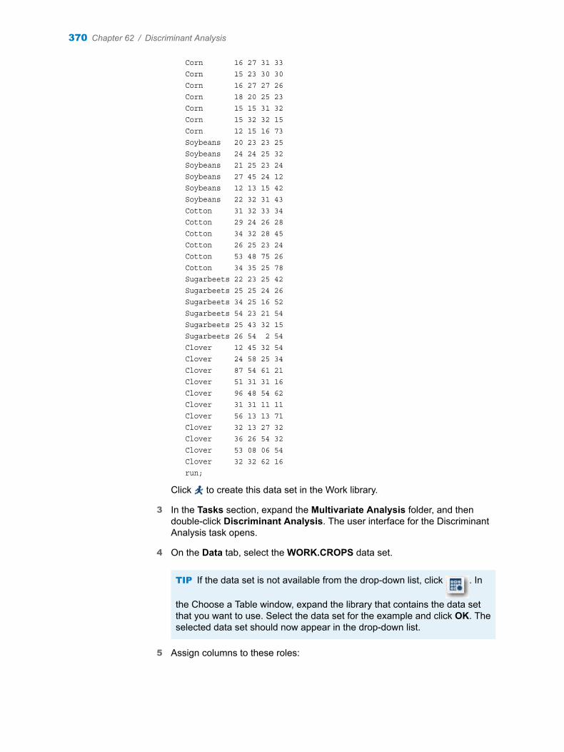
Corn 16 27 31 33Corn 15 23 30 30Corn 16 27 27 26Corn 18 20 25 23Corn 15 15 31 32Corn 15 32 32 15Corn 12 15 16 73Soybeans 20 23 23 25Soybeans 24 24 25 32Soybeans 21 25 23 24Soybeans 27 45 24 12Soybeans 12 13 15 42Soybeans 22 32 31 43Cotton 31 32 33 34Cotton 29 24 26 28Cotton 34 32 28 45Cotton 26 25 23 24Cotton 53 48 75 26Cotton 34 35 25 78Sugarbeets 22 23 25 42Sugarbeets 25 25 24 26Sugarbeets 34 25 16 52Sugarbeets 54 23 21 54Sugarbeets 25 43 32 15Sugarbeets 26 54 2 54Clover 12 45 32 54Clover 24 58 25 34Clover 87 54 61 21Clover 51 31 31 16Clover 96 48 54 62Clover 31 31 11 11Clover 56 13 13 71Clover 32 13 27 32Clover 36 26 54 32Clover 53 08 06 54Clover 32 32 62 16run;
Click to create this data set in the Work library.
3 In the Tasks section, expand the Multivariate Analysis folder, and then double-click Discriminant Analysis. The user interface for the Discriminant Analysis task opens.
4 On the Data tab, select the WORK.CROPS data set.
TIP If the data set is not available from the drop-down list, click . In
the Choose a Table window, expand the library that contains the data set that you want to use. Select the data set for the example and click OK. The selected data set should now appear in the drop-down list.
5 Assign columns to these roles:
370 Chapter 62 / Discriminant Analysis
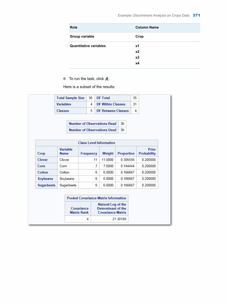
Role Column Name
Group variable Crop
Quantitative variables x1x2x3x4
6 To run the task, click .
Here is a subset of the results:
Example: Discriminant Analysis on Crops Data 371
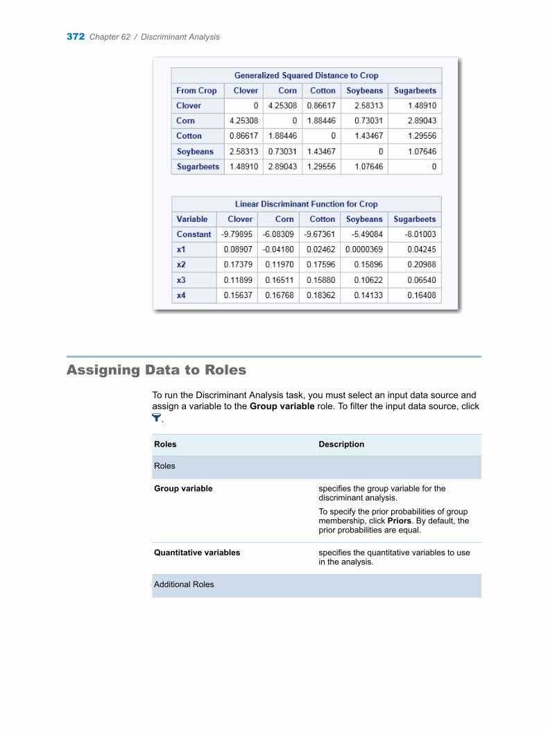
Assigning Data to Roles
To run the Discriminant Analysis task, you must select an input data source and assign a variable to the Group variable role. To filter the input data source, click
.
Roles Description
Roles
Group variable specifies the group variable for the discriminant analysis.
To specify the prior probabilities of group membership, click Priors. By default, the prior probabilities are equal.
Quantitative variables specifies the quantitative variables to use in the analysis.
Additional Roles
372 Chapter 62 / Discriminant Analysis
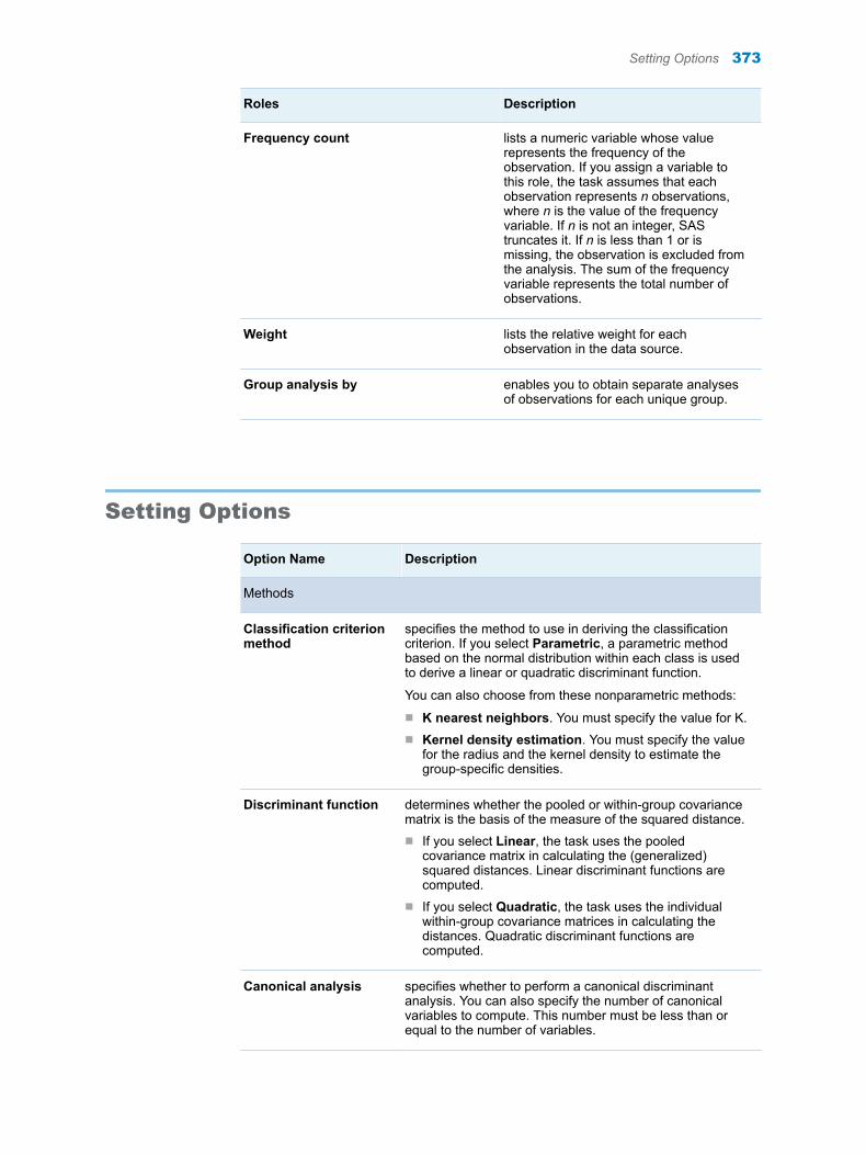
Roles Description
Frequency count lists a numeric variable whose value represents the frequency of the observation. If you assign a variable to this role, the task assumes that each observation represents n observations, where n is the value of the frequency variable. If n is not an integer, SAS truncates it. If n is less than 1 or is missing, the observation is excluded from the analysis. The sum of the frequency variable represents the total number of observations.
Weight lists the relative weight for each observation in the data source.
Group analysis by enables you to obtain separate analyses of observations for each unique group.
Setting Options
Option Name Description
Methods
Classification criterion method
specifies the method to use in deriving the classification criterion. If you select Parametric, a parametric method based on the normal distribution within each class is used to derive a linear or quadratic discriminant function.
You can also choose from these nonparametric methods:
n K nearest neighbors. You must specify the value for K.n Kernel density estimation. You must specify the value
for the radius and the kernel density to estimate the group-specific densities.
Discriminant function determines whether the pooled or within-group covariance matrix is the basis of the measure of the squared distance.n If you select Linear, the task uses the pooled
covariance matrix in calculating the (generalized) squared distances. Linear discriminant functions are computed.
n If you select Quadratic, the task uses the individual within-group covariance matrices in calculating the distances. Quadratic discriminant functions are computed.
Canonical analysis specifies whether to perform a canonical discriminant analysis. You can also specify the number of canonical variables to compute. This number must be less than or equal to the number of variables.
Setting Options 373
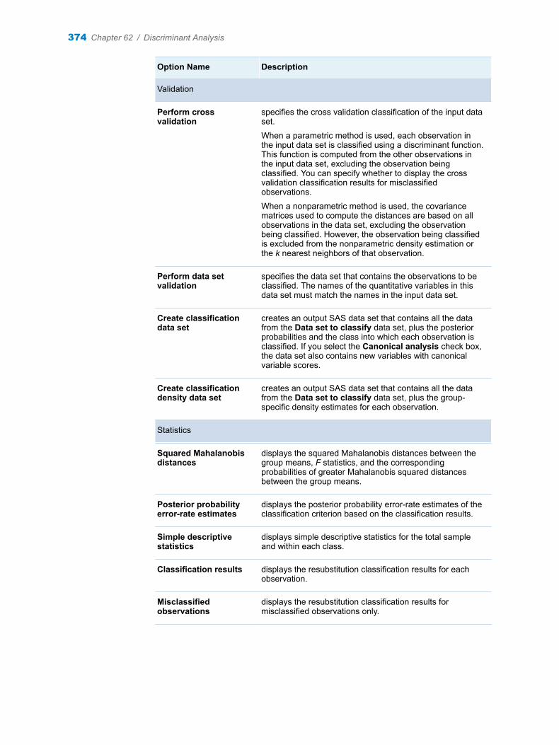
Option Name Description
Validation
Perform cross validation
specifies the cross validation classification of the input data set.
When a parametric method is used, each observation in the input data set is classified using a discriminant function. This function is computed from the other observations in the input data set, excluding the observation being classified. You can specify whether to display the cross validation classification results for misclassified observations.
When a nonparametric method is used, the covariance matrices used to compute the distances are based on all observations in the data set, excluding the observation being classified. However, the observation being classified is excluded from the nonparametric density estimation or the k nearest neighbors of that observation.
Perform data set validation
specifies the data set that contains the observations to be classified. The names of the quantitative variables in this data set must match the names in the input data set.
Create classification data set
creates an output SAS data set that contains all the data from the Data set to classify data set, plus the posterior probabilities and the class into which each observation is classified. If you select the Canonical analysis check box, the data set also contains new variables with canonical variable scores.
Create classification density data set
creates an output SAS data set that contains all the data from the Data set to classify data set, plus the group-specific density estimates for each observation.
Statistics
Squared Mahalanobis distances
displays the squared Mahalanobis distances between the group means, F statistics, and the corresponding probabilities of greater Mahalanobis squared distances between the group means.
Posterior probability error-rate estimates
displays the posterior probability error-rate estimates of the classification criterion based on the classification results.
Simple descriptive statistics
displays simple descriptive statistics for the total sample and within each class.
Classification results displays the resubstitution classification results for each observation.
Misclassified observations
displays the resubstitution classification results for misclassified observations only.
374 Chapter 62 / Discriminant Analysis
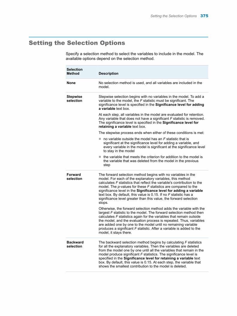
Setting the Selection Options
Specify a selection method to select the variables to include in the model. The available options depend on the selection method.
Selection Method Description
None No selection method is used, and all variables are included in the model.
Stepwise selection
Stepwise selection begins with no variables in the model. To add a variable to the model, the F statistic must be significant. The significance level is specified in the Significance level for adding a variable text box.
At each step, all variables in the model are evaluated for retention. Any variable that does not have a significant F statistic is removed. The significance level is specified in the Significance level for retaining a variable text box.
The stepwise process ends when either of these conditions is met:
n no variable outside the model has an F statistic that is significant at the significance level for adding a variable, and every variable in the model is significant at the significance level to stay in the model
n the variable that meets the criterion for addition to the model is the variable that was deleted from the model in the previous step
Forward selection
The forward selection method begins with no variables in the model. For each of the explanatory variables, this method calculates F statistics that reflect the variable's contribution to the model. The p-values for these F statistics are compared to the significance level in the Significance level for adding a variable text box. By default, this value is 0.15. If no F statistic has a significance level greater than this value, the forward selection stops.
Otherwise, the forward selection method adds the variable with the largest F statistic to the model. The forward selection method then calculates F statistics again for the variables that remain outside the model, and the evaluation process is repeated. Thus, variables are added one by one to the model until no remaining variable produces a significant F statistic. After a variable is added to the model, it stays there.
Backward selection
The backward selection method begins by calculating F statistics for all the explanatory variables. Then the variables are deleted from the model one by one until all the variables that remain in the model produce significant F statistics. The significance level is specified in the Significance level for retaining a variable text box. By default, this value is 0.15. At each step, the variable that shows the smallest contribution to the model is deleted.
Setting the Selection Options 375

Setting the Output Options
You can choose to create these data sets:
n classification results
n statistics
n density
376 Chapter 62 / Discriminant Analysis
63Correspondence Analysis
About the Correspondence Analysis Task . . . . . . . . . . . . . . . . . . . . . . . . . . . . . . . . . 377
Example: Correspondence Analysis . . . . . . . . . . . . . . . . . . . . . . . . . . . . . . . . . . . . . . . 377
Assigning Data to Roles . . . . . . . . . . . . . . . . . . . . . . . . . . . . . . . . . . . . . . . . . . . . . . . . . . . 379Simple Correspondence Analysis of Raw Data . . . . . . . . . . . . . . . . . . . . . . . . . . . . 379Multiple Correspondence Analysis of Raw Data . . . . . . . . . . . . . . . . . . . . . . . . . . . 380Simple Correspondence Analysis of Table Data . . . . . . . . . . . . . . . . . . . . . . . . . . . 381Multiple Correspondence Analysis of Table Data . . . . . . . . . . . . . . . . . . . . . . . . . . . 382
Setting Options . . . . . . . . . . . . . . . . . . . . . . . . . . . . . . . . . . . . . . . . . . . . . . . . . . . . . . . . . . . . 383
Setting the Output Options . . . . . . . . . . . . . . . . . . . . . . . . . . . . . . . . . . . . . . . . . . . . . . . . 384
About the Correspondence Analysis Task
The Correspondence Analysis task performs simple or multiple correspondence analysis of qualitative data. You can specify either raw data or table data for the input data source.
Example: Correspondence Analysis
To create this example:
1 In SAS Studio, click and select New SAS Program.
2 Copy and paste this code into the Program tab.
data PhD; input Science $ 1-21 y1973-y1978; label y1973 = '1973' y1974 = '1974' y1975 = '1975' y1976 = '1976' y1977 = '1977' y1978 = '1978';datalines;Life Sciences 4489 4303 4402 4350 4266 4361Physical Sciences 4101 3800 3749 3572 3410 3234Social Sciences 3354 3286 3344 3278 3137 3008Behavioral Sciences 2444 2587 2749 2878 2960 3049Engineering 3338 3144 2959 2791 2641 2432
377
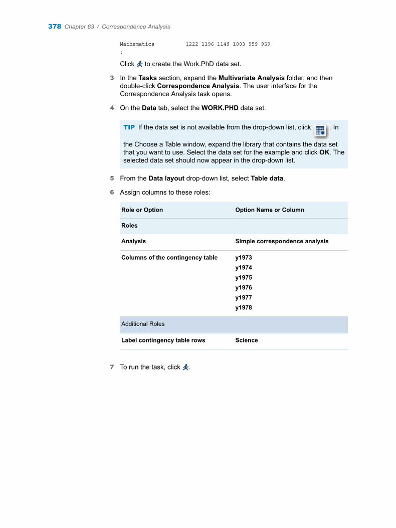
Mathematics 1222 1196 1149 1003 959 959;
Click to create the Work.PhD data set.
3 In the Tasks section, expand the Multivariate Analysis folder, and then double-click Correspondence Analysis. The user interface for the Correspondence Analysis task opens.
4 On the Data tab, select the WORK.PHD data set.
TIP If the data set is not available from the drop-down list, click . In
the Choose a Table window, expand the library that contains the data set that you want to use. Select the data set for the example and click OK. The selected data set should now appear in the drop-down list.
5 From the Data layout drop-down list, select Table data.
6 Assign columns to these roles:
Role or Option Option Name or Column
Roles
Analysis Simple correspondence analysis
Columns of the contingency table y1973y1974y1975y1976y1977y1978
Additional Roles
Label contingency table rows Science
7 To run the task, click .
378 Chapter 63 / Correspondence Analysis
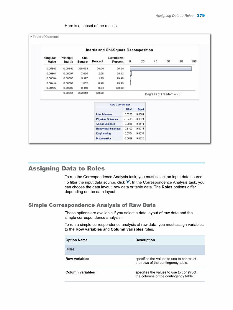
Here is a subset of the results:
Assigning Data to RolesTo run the Correspondence Analysis task, you must select an input data source. To filter the input data source, click . In the Correspondence Analysis task, you can choose the data layout: raw data or table data. The Roles options differ depending on the data layout.
Simple Correspondence Analysis of Raw Data
These options are available if you select a data layout of raw data and the simple correspondence analysis.
To run a simple correspondence analysis of raw data, you must assign variables to the Row variables and Column variables roles.
Option Name Description
Roles
Row variables specifies the values to use to construct the rows of the contingency table.
Column variables specifies the values to use to construct the columns of the contingency table.
Assigning Data to Roles 379
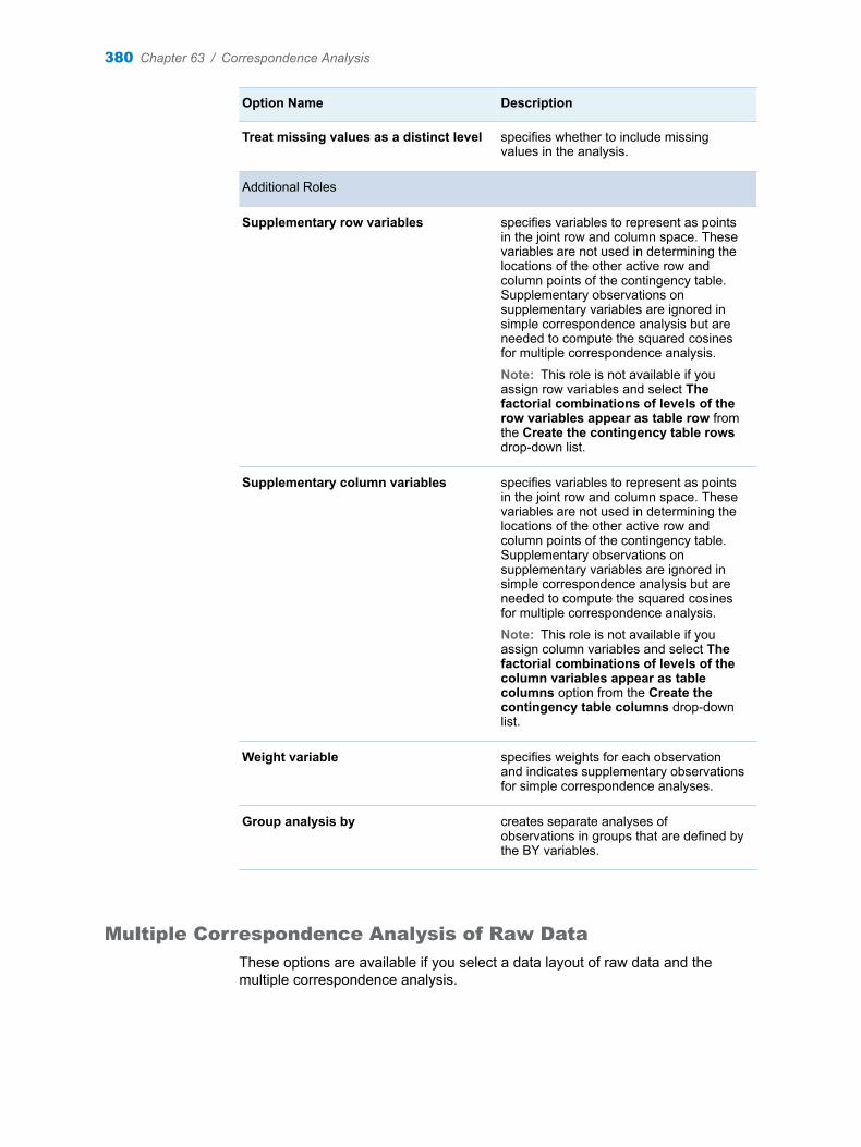
Option Name Description
Treat missing values as a distinct level specifies whether to include missing values in the analysis.
Additional Roles
Supplementary row variables specifies variables to represent as points in the joint row and column space. These variables are not used in determining the locations of the other active row and column points of the contingency table. Supplementary observations on supplementary variables are ignored in simple correspondence analysis but are needed to compute the squared cosines for multiple correspondence analysis.
Note: This role is not available if you assign row variables and select The factorial combinations of levels of the row variables appear as table row from the Create the contingency table rows drop-down list.
Supplementary column variables specifies variables to represent as points in the joint row and column space. These variables are not used in determining the locations of the other active row and column points of the contingency table. Supplementary observations on supplementary variables are ignored in simple correspondence analysis but are needed to compute the squared cosines for multiple correspondence analysis.
Note: This role is not available if you assign column variables and select The factorial combinations of levels of the column variables appear as table columns option from the Create the contingency table columns drop-down list.
Weight variable specifies weights for each observation and indicates supplementary observations for simple correspondence analyses.
Group analysis by creates separate analyses of observations in groups that are defined by the BY variables.
Multiple Correspondence Analysis of Raw Data
These options are available if you select a data layout of raw data and the multiple correspondence analysis.
380 Chapter 63 / Correspondence Analysis

To run a multiple correspondence analysis of raw data, you must assign a variable to the Column variables role.
Option Name Description
Roles
Column variables specifies the values to use to construct the columns of the contingency table. You must assign at least two variables to this role.
Treat missing values as a distinct level specifies whether to include missing values in the analysis.
Additional Roles
Supplementary column variables specifies variables to represent as points in the joint row and column space. These variables are not used in determining the locations of the other active row and column points of the contingency table. Supplementary observations on supplementary variables are ignored in simple correspondence analysis but are needed to compute the squared cosines for multiple correspondence analysis.
Weight variable specifies weights for each observation and indicates supplementary observations for simple correspondence analyses.
Group analysis by creates separate analyses of observations in groups that are defined by the BY variables.
Simple Correspondence Analysis of Table Data
These options are available if you select a data layout of table data and the simple correspondence analysis.
To run a simple correspondence analysis of table data, you must assign at least two variables to the Columns of the contingency table role.
Option Name Description
Roles
Columns of the contingency table reads an existing contingency table, binary indicator matrix, fuzzy-coded indicator matrix, or Burt table, rather than raw data.
Additional Roles
Assigning Data to Roles 381
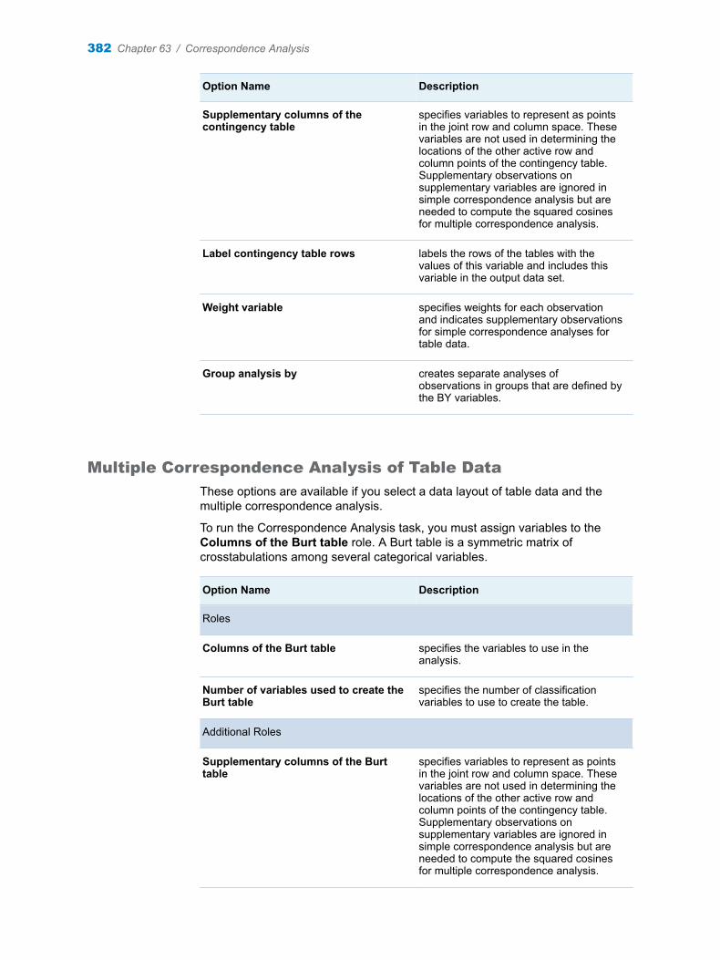
Option Name Description
Supplementary columns of the contingency table
specifies variables to represent as points in the joint row and column space. These variables are not used in determining the locations of the other active row and column points of the contingency table. Supplementary observations on supplementary variables are ignored in simple correspondence analysis but are needed to compute the squared cosines for multiple correspondence analysis.
Label contingency table rows labels the rows of the tables with the values of this variable and includes this variable in the output data set.
Weight variable specifies weights for each observation and indicates supplementary observations for simple correspondence analyses for table data.
Group analysis by creates separate analyses of observations in groups that are defined by the BY variables.
Multiple Correspondence Analysis of Table Data
These options are available if you select a data layout of table data and the multiple correspondence analysis.
To run the Correspondence Analysis task, you must assign variables to the Columns of the Burt table role. A Burt table is a symmetric matrix of crosstabulations among several categorical variables.
Option Name Description
Roles
Columns of the Burt table specifies the variables to use in the analysis.
Number of variables used to create the Burt table
specifies the number of classification variables to use to create the table.
Additional Roles
Supplementary columns of the Burt table
specifies variables to represent as points in the joint row and column space. These variables are not used in determining the locations of the other active row and column points of the contingency table. Supplementary observations on supplementary variables are ignored in simple correspondence analysis but are needed to compute the squared cosines for multiple correspondence analysis.
382 Chapter 63 / Correspondence Analysis

Option Name Description
Group analysis by creates separate analyses of observations in groups that are defined by the BY variables.
Setting Options
Option Name Description
Methods
Number of dimensions specifies the number of dimensions or axes to use.
Details
Display as frequencies or percents specifies whether to include the frequencies, percents, or both in the output.
Standardize coordinates specifies whether to standardize the coordinates. A standard correspondence analysis jointly displays the principal row and column coordinates. Row coordinates are computed from the row profile matrix, and column coordinates are computed from the column profile matrix.
Statistics
The available statistics depend on the type of analysis that you are performing. You can choose what statistics to display in the results.
For a simple correspondence analysis, these statistics are available:
n coordinates—row and columnn profiles—row and columnn inertia—P-value for chi-squaren frequencies—observed, expected, deviation, and cell contribution to chi-square
For a multiple correspondence analysis, these statistics are available:
n column coordinatesn column profilen inertia—P-value for chi-square, Benzécri adjusted inertia, and Greenacre adjusted
inertian frequencies—observed, expected, deviation, and cell contribution to chi-square
Plots
By default, the inertia plot and configuration plot are included in the output. You can choose to remove one or both of these plots from the output.
Setting Options 383

Setting the Output Options
You can specify whether to create a coordinates data set.
384 Chapter 63 / Correspondence Analysis
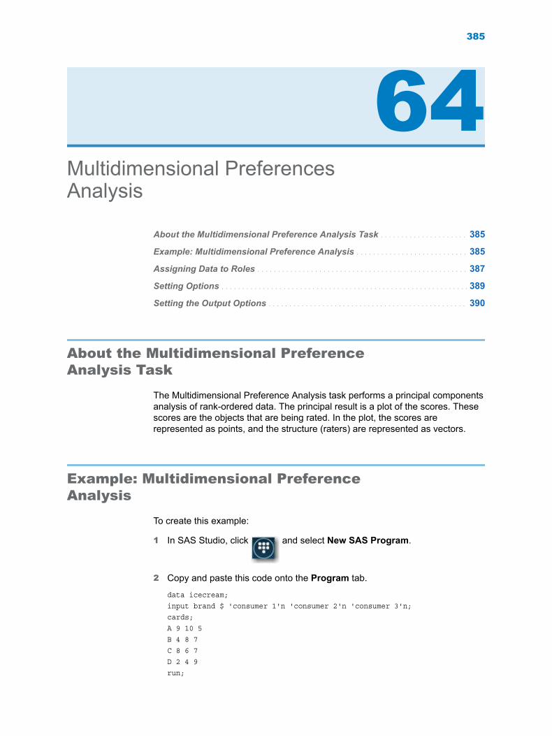
64Multidimensional Preferences Analysis
About the Multidimensional Preference Analysis Task . . . . . . . . . . . . . . . . . . . . . 385
Example: Multidimensional Preference Analysis . . . . . . . . . . . . . . . . . . . . . . . . . . . 385
Assigning Data to Roles . . . . . . . . . . . . . . . . . . . . . . . . . . . . . . . . . . . . . . . . . . . . . . . . . . . 387
Setting Options . . . . . . . . . . . . . . . . . . . . . . . . . . . . . . . . . . . . . . . . . . . . . . . . . . . . . . . . . . . . 389
Setting the Output Options . . . . . . . . . . . . . . . . . . . . . . . . . . . . . . . . . . . . . . . . . . . . . . . . 390
About the Multidimensional Preference Analysis Task
The Multidimensional Preference Analysis task performs a principal components analysis of rank-ordered data. The principal result is a plot of the scores. These scores are the objects that are being rated. In the plot, the scores are represented as points, and the structure (raters) are represented as vectors.
Example: Multidimensional Preference Analysis
To create this example:
1 In SAS Studio, click and select New SAS Program.
2 Copy and paste this code onto the Program tab.
data icecream;input brand $ 'consumer 1'n 'consumer 2'n 'consumer 3'n;cards;A 9 10 5B 4 8 7C 8 6 7D 2 4 9run;
385
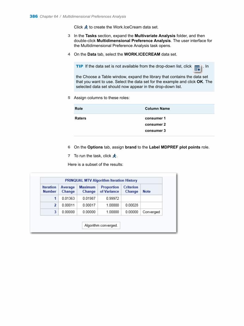
Click to create the Work.IceCream data set.
3 In the Tasks section, expand the Multivariate Analysis folder, and then double-click Multidimensional Preference Analysis. The user interface for the Multidimensional Preference Analysis task opens.
4 On the Data tab, select the WORK.ICECREAM data set.
TIP If the data set is not available from the drop-down list, click . In
the Choose a Table window, expand the library that contains the data set that you want to use. Select the data set for the example and click OK. The selected data set should now appear in the drop-down list.
5 Assign columns to these roles:
Role Column Name
Raters consumer 1consumer 2consumer 3
6 On the Options tab, assign brand to the Label MDPREF plot points role.
7 To run the task, click .
Here is a subset of the results:
386 Chapter 64 / Multidimensional Preferences Analysis
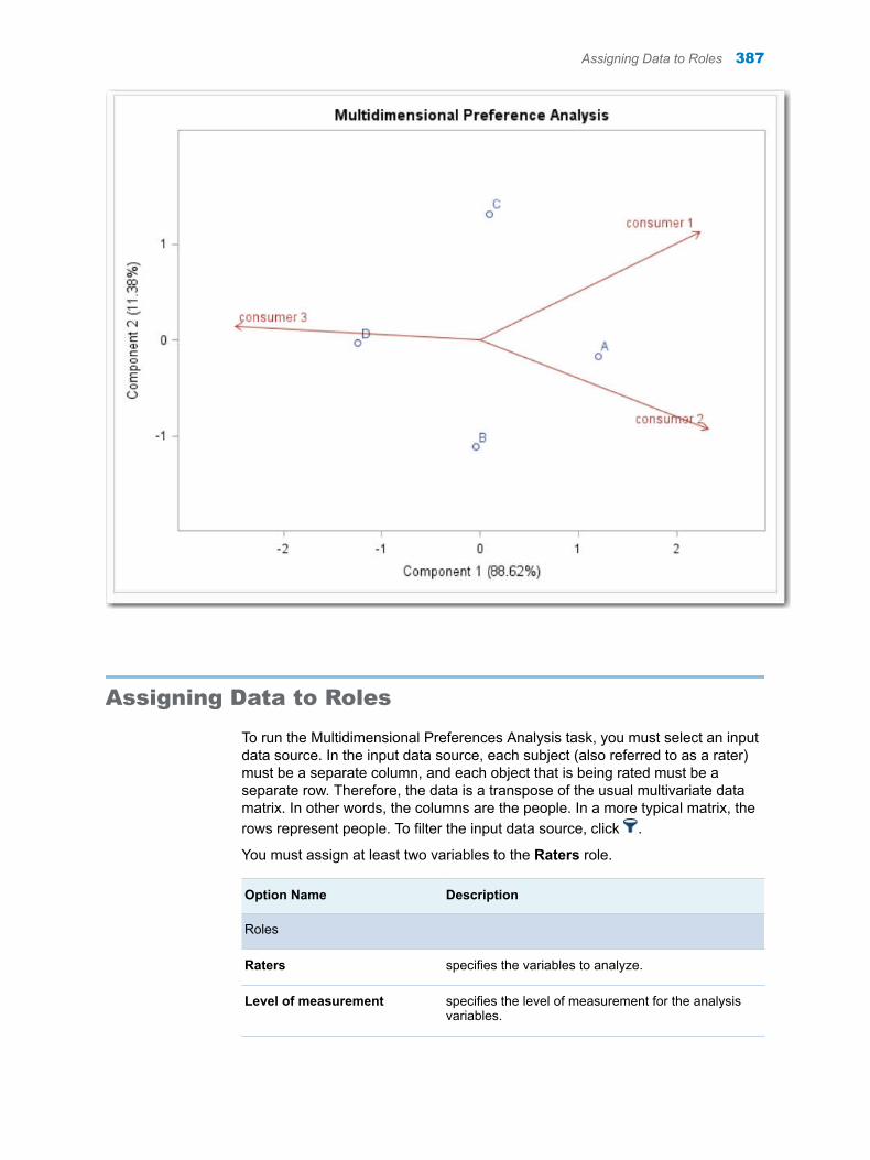
Assigning Data to Roles
To run the Multidimensional Preferences Analysis task, you must select an input data source. In the input data source, each subject (also referred to as a rater) must be a separate column, and each object that is being rated must be a separate row. Therefore, the data is a transpose of the usual multivariate data matrix. In other words, the columns are the people. In a more typical matrix, the rows represent people. To filter the input data source, click .
You must assign at least two variables to the Raters role.
Option Name Description
Roles
Raters specifies the variables to analyze.
Level of measurement specifies the level of measurement for the analysis variables.
Assigning Data to Roles 387
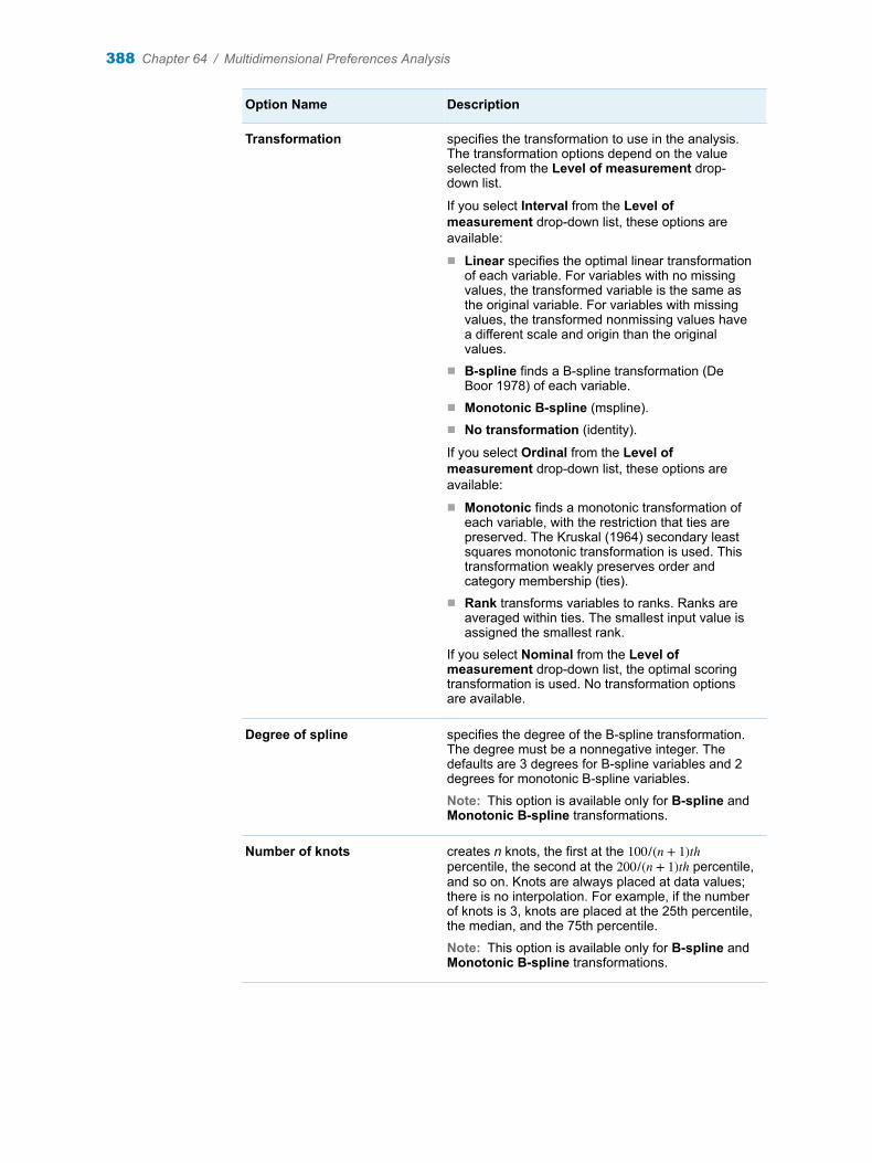
Option Name Description
Transformation specifies the transformation to use in the analysis. The transformation options depend on the value selected from the Level of measurement drop-down list.
If you select Interval from the Level of measurement drop-down list, these options are available:
n Linear specifies the optimal linear transformation of each variable. For variables with no missing values, the transformed variable is the same as the original variable. For variables with missing values, the transformed nonmissing values have a different scale and origin than the original values.
n B-spline finds a B-spline transformation (De Boor 1978) of each variable.
n Monotonic B-spline (mspline).n No transformation (identity).
If you select Ordinal from the Level of measurement drop-down list, these options are available:
n Monotonic finds a monotonic transformation of each variable, with the restriction that ties are preserved. The Kruskal (1964) secondary least squares monotonic transformation is used. This transformation weakly preserves order and category membership (ties).
n Rank transforms variables to ranks. Ranks are averaged within ties. The smallest input value is assigned the smallest rank.
If you select Nominal from the Level of measurement drop-down list, the optimal scoring transformation is used. No transformation options are available.
Degree of spline specifies the degree of the B-spline transformation. The degree must be a nonnegative integer. The defaults are 3 degrees for B-spline variables and 2 degrees for monotonic B-spline variables.
Note: This option is available only for B-spline and Monotonic B-spline transformations.
Number of knots creates n knots, the first at the 100/ n + 1 thpercentile, the second at the 200/ n + 1 th percentile, and so on. Knots are always placed at data values; there is no interpolation. For example, if the number of knots is 3, knots are placed at the 25th percentile, the median, and the 75th percentile.
Note: This option is available only for B-spline and Monotonic B-spline transformations.
388 Chapter 64 / Multidimensional Preferences Analysis
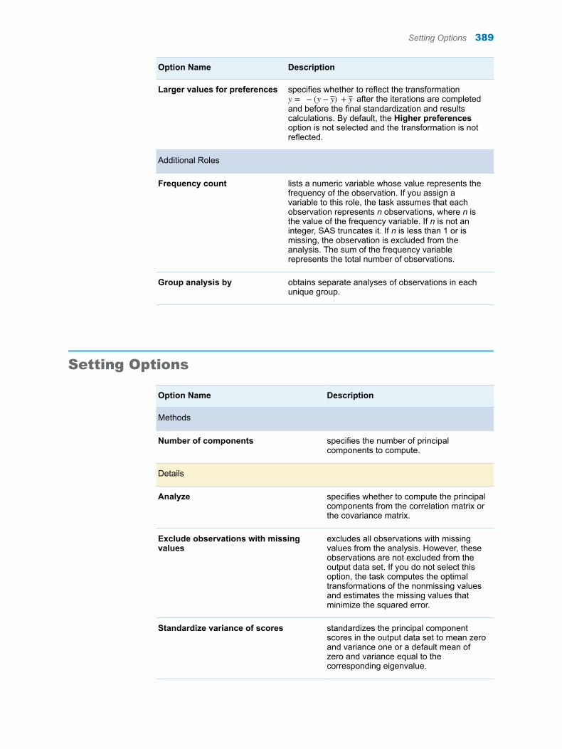
Option Name Description
Larger values for preferences specifies whether to reflect the transformation y = − y − y + y after the iterations are completed and before the final standardization and results calculations. By default, the Higher preferences option is not selected and the transformation is not reflected.
Additional Roles
Frequency count lists a numeric variable whose value represents the frequency of the observation. If you assign a variable to this role, the task assumes that each observation represents n observations, where n is the value of the frequency variable. If n is not an integer, SAS truncates it. If n is less than 1 or is missing, the observation is excluded from the analysis. The sum of the frequency variable represents the total number of observations.
Group analysis by obtains separate analyses of observations in each unique group.
Setting Options
Option Name Description
Methods
Number of components specifies the number of principal components to compute.
Details
Analyze specifies whether to compute the principal components from the correlation matrix or the covariance matrix.
Exclude observations with missing values
excludes all observations with missing values from the analysis. However, these observations are not excluded from the output data set. If you do not select this option, the task computes the optimal transformations of the nonmissing values and estimates the missing values that minimize the squared error.
Standardize variance of scores standardizes the principal component scores in the output data set to mean zero and variance one or a default mean of zero and variance equal to the corresponding eigenvalue.
Setting Options 389
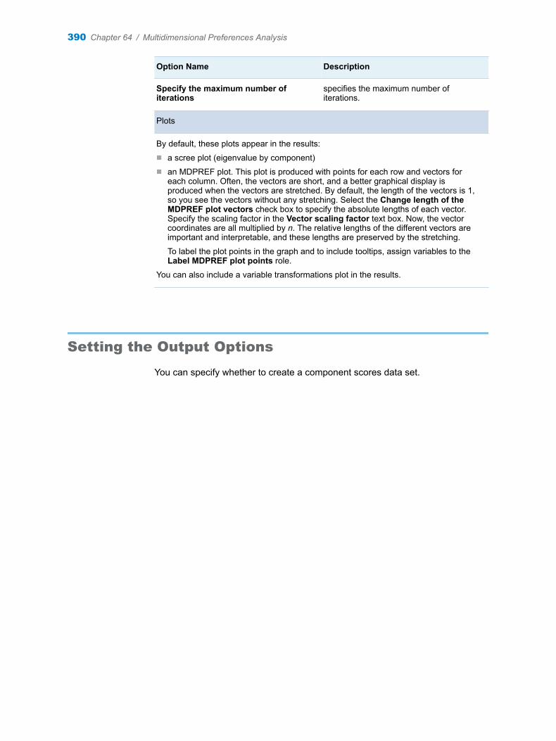
Option Name Description
Specify the maximum number of iterations
specifies the maximum number of iterations.
Plots
By default, these plots appear in the results:n a scree plot (eigenvalue by component)n an MDPREF plot. This plot is produced with points for each row and vectors for
each column. Often, the vectors are short, and a better graphical display is produced when the vectors are stretched. By default, the length of the vectors is 1, so you see the vectors without any stretching. Select the Change length of the MDPREF plot vectors check box to specify the absolute lengths of each vector. Specify the scaling factor in the Vector scaling factor text box. Now, the vector coordinates are all multiplied by n. The relative lengths of the different vectors are important and interpretable, and these lengths are preserved by the stretching.
To label the plot points in the graph and to include tooltips, assign variables to the Label MDPREF plot points role.
You can also include a variable transformations plot in the results.
Setting the Output Options
You can specify whether to create a component scores data set.
390 Chapter 64 / Multidimensional Preferences Analysis

Part 8
Econometrics Tasks
Chapter 65Causal Models . . . . . . . . . . . . . . . . . . . . . . . . . . . . . . . . . . . . . . . . . . . . . . . . . . 393
Chapter 66Cross-sectional Data Models . . . . . . . . . . . . . . . . . . . . . . . . . . . . . . . . . . . . . 403
Chapter 67Panel Data Models . . . . . . . . . . . . . . . . . . . . . . . . . . . . . . . . . . . . . . . . . . . . . . . 435
Chapter 68Time Series Analysis . . . . . . . . . . . . . . . . . . . . . . . . . . . . . . . . . . . . . . . . . . . . 469
391

392

65Causal Models
About the Causal Models Task . . . . . . . . . . . . . . . . . . . . . . . . . . . . . . . . . . . . . . . . . . . . . 393
Two-Stage Least Squares . . . . . . . . . . . . . . . . . . . . . . . . . . . . . . . . . . . . . . . . . . . . . . . . . . 393Example: Two-Stage Least Squares . . . . . . . . . . . . . . . . . . . . . . . . . . . . . . . . . . . . . . 393Assigning Data to Roles . . . . . . . . . . . . . . . . . . . . . . . . . . . . . . . . . . . . . . . . . . . . . . . . . 395Setting Options . . . . . . . . . . . . . . . . . . . . . . . . . . . . . . . . . . . . . . . . . . . . . . . . . . . . . . . . . 396Creating the Output Data Sets . . . . . . . . . . . . . . . . . . . . . . . . . . . . . . . . . . . . . . . . . . . 397
Heckman’s Two-Step Selection Method . . . . . . . . . . . . . . . . . . . . . . . . . . . . . . . . . . . . 397About Heckman’s Two-Step Selection Method . . . . . . . . . . . . . . . . . . . . . . . . . . . . . 397Example: Heckman’s Two-Step Selection Method . . . . . . . . . . . . . . . . . . . . . . . . . 398Assigning Data to Roles . . . . . . . . . . . . . . . . . . . . . . . . . . . . . . . . . . . . . . . . . . . . . . . . . 399Setting Options . . . . . . . . . . . . . . . . . . . . . . . . . . . . . . . . . . . . . . . . . . . . . . . . . . . . . . . . . 400Creating the Output Data Sets . . . . . . . . . . . . . . . . . . . . . . . . . . . . . . . . . . . . . . . . . . . 401
About the Causal Models Task
Causal models deal with a special type of cross-sectional data that has endogenous variables. An endogenous variable is a factor in a causal model or causal system whose value is determined by the states of other variables in the system. (The value of an exogenous variable is independent from the states of other variables in the system.)
With the Causal Models task, you can use these two techniques:
n two-stage least squares
n Heckman’s two-step selection method
Two-Stage Least Squares
Example: Two-Stage Least Squares
To create this example:
1 In the Tasks section, expand the Econometrics folder, and then double-click Causal Models. The user interface for the Causal Models task opens.
393
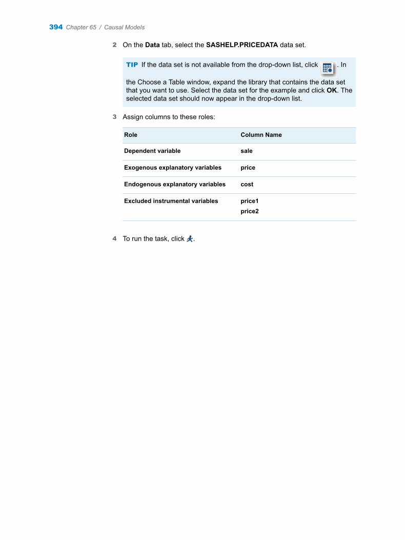
2 On the Data tab, select the SASHELP.PRICEDATA data set.
TIP If the data set is not available from the drop-down list, click . In
the Choose a Table window, expand the library that contains the data set that you want to use. Select the data set for the example and click OK. The selected data set should now appear in the drop-down list.
3 Assign columns to these roles:
Role Column Name
Dependent variable sale
Exogenous explanatory variables price
Endogenous explanatory variables cost
Excluded instrumental variables price1price2
4 To run the task, click .
394 Chapter 65 / Causal Models
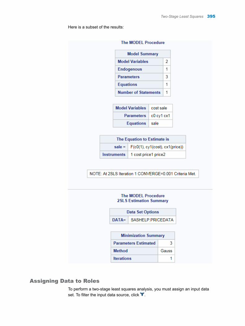
Here is a subset of the results:
Assigning Data to Roles
To perform a two-stage least squares analysis, you must assign an input data set. To filter the input data source, click .
Two-Stage Least Squares 395
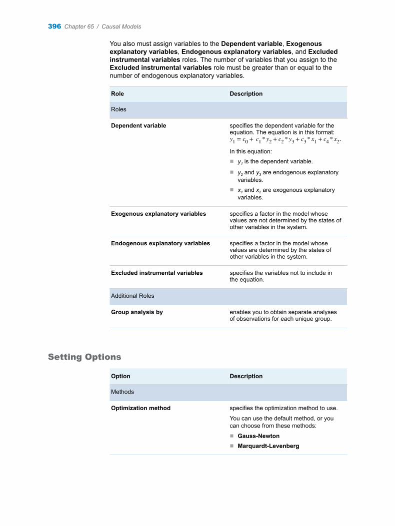
You also must assign variables to the Dependent variable, Exogenous explanatory variables, Endogenous explanatory variables, and Excluded instrumental variables roles. The number of variables that you assign to the Excluded instrumental variables role must be greater than or equal to the number of endogenous explanatory variables.
Role Description
Roles
Dependent variable specifies the dependent variable for the equation. The equation is in this format:y1 = c0 + c1 * y2 + c2 * y3 + c3 * x1 + c4 * x2.
In this equation:n y1 is the dependent variable.
n y2 and y3 are endogenous explanatory variables.
n x1 and x2 are exogenous explanatory variables.
Exogenous explanatory variables specifies a factor in the model whose values are not determined by the states of other variables in the system.
Endogenous explanatory variables specifies a factor in the model whose values are determined by the states of other variables in the system.
Excluded instrumental variables specifies the variables not to include in the equation.
Additional Roles
Group analysis by enables you to obtain separate analyses of observations for each unique group.
Setting Options
Option Description
Methods
Optimization method specifies the optimization method to use.
You can use the default method, or you can choose from these methods:
n Gauss-Newtonn Marquardt-Levenberg
396 Chapter 65 / Causal Models
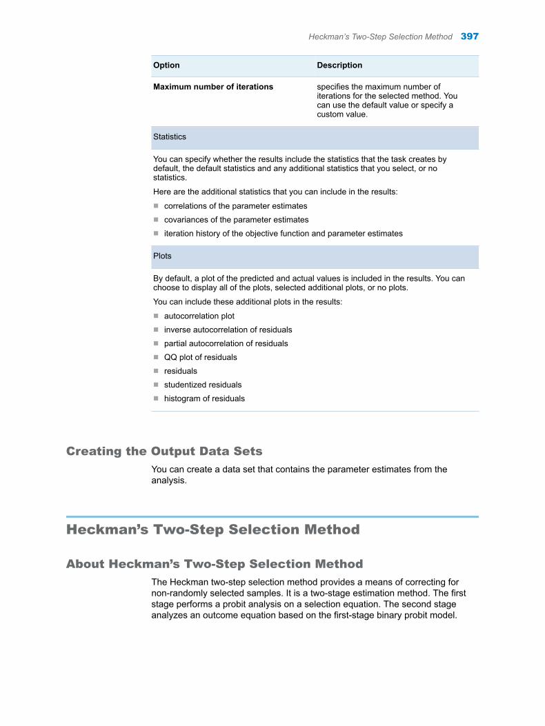
Option Description
Maximum number of iterations specifies the maximum number of iterations for the selected method. You can use the default value or specify a custom value.
Statistics
You can specify whether the results include the statistics that the task creates by default, the default statistics and any additional statistics that you select, or no statistics.
Here are the additional statistics that you can include in the results:
n correlations of the parameter estimatesn covariances of the parameter estimatesn iteration history of the objective function and parameter estimates
Plots
By default, a plot of the predicted and actual values is included in the results. You can choose to display all of the plots, selected additional plots, or no plots.
You can include these additional plots in the results:
n autocorrelation plotn inverse autocorrelation of residualsn partial autocorrelation of residualsn QQ plot of residualsn residualsn studentized residualsn histogram of residuals
Creating the Output Data Sets
You can create a data set that contains the parameter estimates from the analysis.
Heckman’s Two-Step Selection Method
About Heckman’s Two-Step Selection Method
The Heckman two-step selection method provides a means of correcting for non-randomly selected samples. It is a two-stage estimation method. The first stage performs a probit analysis on a selection equation. The second stage analyzes an outcome equation based on the first-stage binary probit model.
Heckman’s Two-Step Selection Method 397
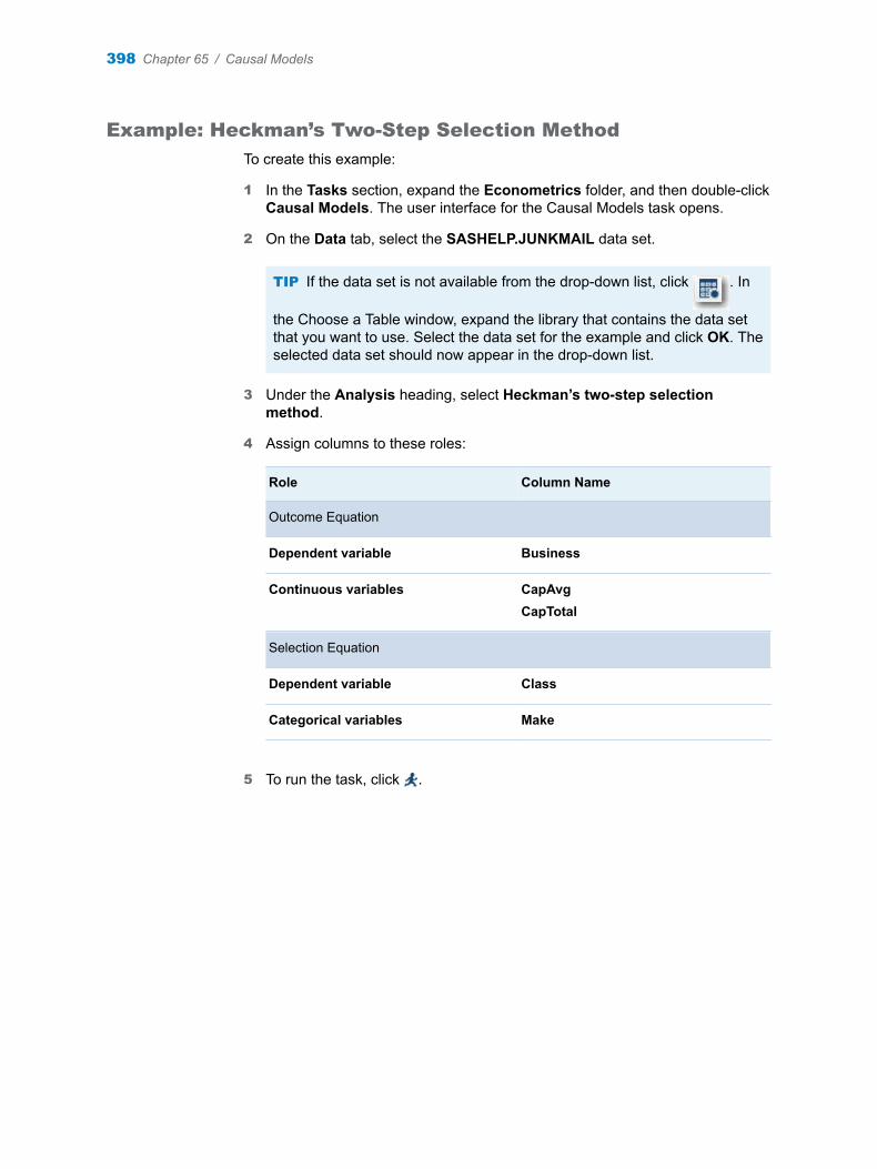
Example: Heckman’s Two-Step Selection Method
To create this example:
1 In the Tasks section, expand the Econometrics folder, and then double-click Causal Models. The user interface for the Causal Models task opens.
2 On the Data tab, select the SASHELP.JUNKMAIL data set.
TIP If the data set is not available from the drop-down list, click . In
the Choose a Table window, expand the library that contains the data set that you want to use. Select the data set for the example and click OK. The selected data set should now appear in the drop-down list.
3 Under the Analysis heading, select Heckman’s two-step selection method.
4 Assign columns to these roles:
Role Column Name
Outcome Equation
Dependent variable Business
Continuous variables CapAvgCapTotal
Selection Equation
Dependent variable Class
Categorical variables Make
5 To run the task, click .
398 Chapter 65 / Causal Models
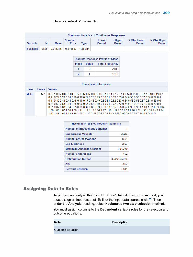
Here is a subset of the results:
Assigning Data to Roles
To perform an analysis that uses Heckman’s two-step selection method, you must assign an input data set. To filter the input data source, click . Then under the Analysis heading, select Heckman’s two-step selection method.
You must assign columns to the Dependent variable roles for the selection and outcome equations.
Role Description
Outcome Equation
Heckman’s Two-Step Selection Method 399
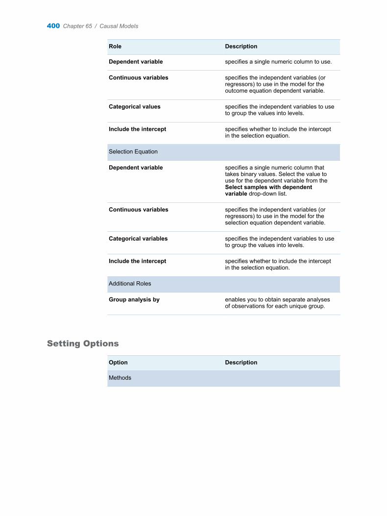
Role Description
Dependent variable specifies a single numeric column to use.
Continuous variables specifies the independent variables (or regressors) to use in the model for the outcome equation dependent variable.
Categorical values specifies the independent variables to use to group the values into levels.
Include the intercept specifies whether to include the intercept in the selection equation.
Selection Equation
Dependent variable specifies a single numeric column that takes binary values. Select the value to use for the dependent variable from the Select samples with dependent variable drop-down list.
Continuous variables specifies the independent variables (or regressors) to use in the model for the selection equation dependent variable.
Categorical variables specifies the independent variables to use to group the values into levels.
Include the intercept specifies whether to include the intercept in the selection equation.
Additional Roles
Group analysis by enables you to obtain separate analyses of observations for each unique group.
Setting Options
Option Description
Methods
400 Chapter 65 / Causal Models
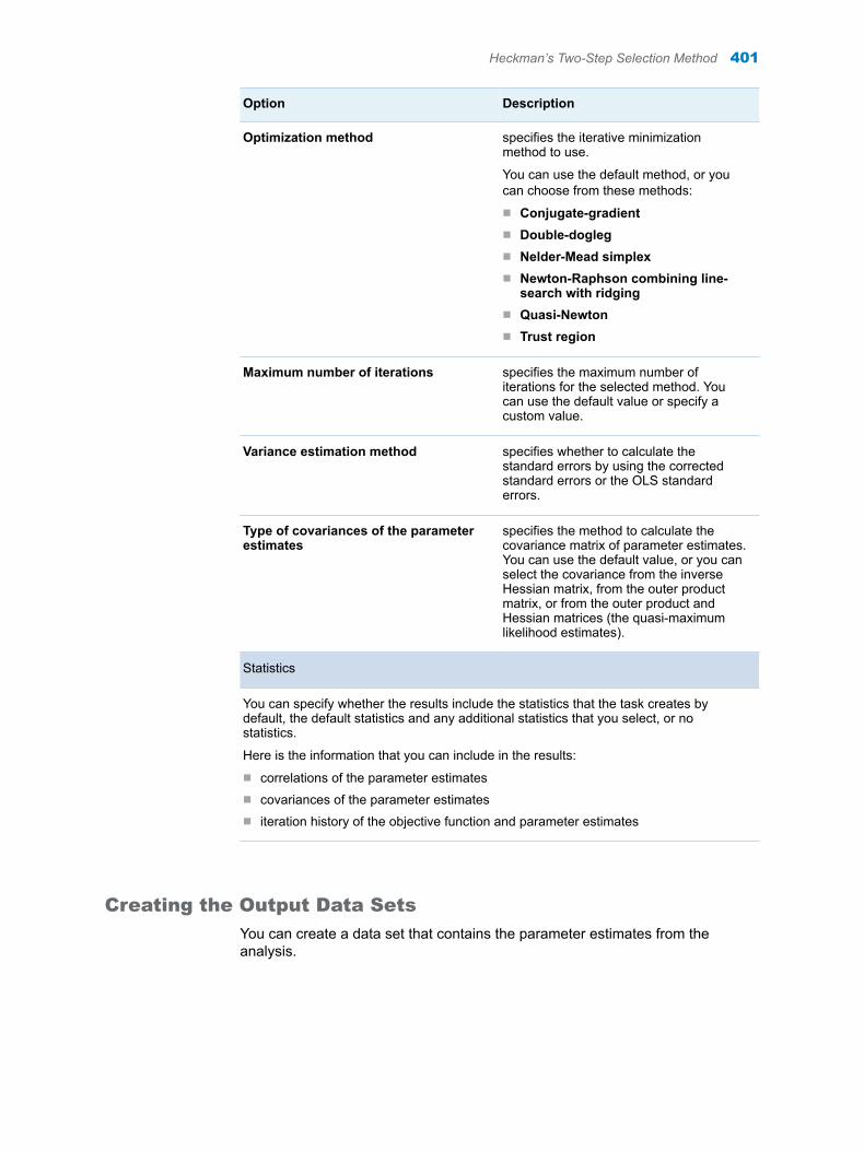
Option Description
Optimization method specifies the iterative minimization method to use.
You can use the default method, or you can choose from these methods:
n Conjugate-gradientn Double-doglegn Nelder-Mead simplexn Newton-Raphson combining line-
search with ridgingn Quasi-Newtonn Trust region
Maximum number of iterations specifies the maximum number of iterations for the selected method. You can use the default value or specify a custom value.
Variance estimation method specifies whether to calculate the standard errors by using the corrected standard errors or the OLS standard errors.
Type of covariances of the parameter estimates
specifies the method to calculate the covariance matrix of parameter estimates. You can use the default value, or you can select the covariance from the inverse Hessian matrix, from the outer product matrix, or from the outer product and Hessian matrices (the quasi-maximum likelihood estimates).
Statistics
You can specify whether the results include the statistics that the task creates by default, the default statistics and any additional statistics that you select, or no statistics.
Here is the information that you can include in the results:
n correlations of the parameter estimatesn covariances of the parameter estimatesn iteration history of the objective function and parameter estimates
Creating the Output Data Sets
You can create a data set that contains the parameter estimates from the analysis.
Heckman’s Two-Step Selection Method 401

402 Chapter 65 / Causal Models

66Cross-sectional Data Models
About the Cross-Sectional Data Models Task . . . . . . . . . . . . . . . . . . . . . . . . . . . . . . 404
Linear Models . . . . . . . . . . . . . . . . . . . . . . . . . . . . . . . . . . . . . . . . . . . . . . . . . . . . . . . . . . . . . 404Example: Linear Regression with Fixed Effects . . . . . . . . . . . . . . . . . . . . . . . . . . . . 404Assigning Data to Roles . . . . . . . . . . . . . . . . . . . . . . . . . . . . . . . . . . . . . . . . . . . . . . . . . 405Setting the Model Options . . . . . . . . . . . . . . . . . . . . . . . . . . . . . . . . . . . . . . . . . . . . . . . 406Setting the Options . . . . . . . . . . . . . . . . . . . . . . . . . . . . . . . . . . . . . . . . . . . . . . . . . . . . . . 407Creating the Output Data Sets . . . . . . . . . . . . . . . . . . . . . . . . . . . . . . . . . . . . . . . . . . . 408
Logit Model . . . . . . . . . . . . . . . . . . . . . . . . . . . . . . . . . . . . . . . . . . . . . . . . . . . . . . . . . . . . . . . 408Example: Logit Model . . . . . . . . . . . . . . . . . . . . . . . . . . . . . . . . . . . . . . . . . . . . . . . . . . . . 408Assigning Data to Roles . . . . . . . . . . . . . . . . . . . . . . . . . . . . . . . . . . . . . . . . . . . . . . . . . 409Setting the Model Options . . . . . . . . . . . . . . . . . . . . . . . . . . . . . . . . . . . . . . . . . . . . . . . 410Setting the Options . . . . . . . . . . . . . . . . . . . . . . . . . . . . . . . . . . . . . . . . . . . . . . . . . . . . . . 411Creating the Output Data Sets . . . . . . . . . . . . . . . . . . . . . . . . . . . . . . . . . . . . . . . . . . . 412
Probit Model . . . . . . . . . . . . . . . . . . . . . . . . . . . . . . . . . . . . . . . . . . . . . . . . . . . . . . . . . . . . . . . 412Example: Probit Model . . . . . . . . . . . . . . . . . . . . . . . . . . . . . . . . . . . . . . . . . . . . . . . . . . . 412Assigning Data to Roles . . . . . . . . . . . . . . . . . . . . . . . . . . . . . . . . . . . . . . . . . . . . . . . . . 414Setting the Model Options . . . . . . . . . . . . . . . . . . . . . . . . . . . . . . . . . . . . . . . . . . . . . . . 415Setting the Options . . . . . . . . . . . . . . . . . . . . . . . . . . . . . . . . . . . . . . . . . . . . . . . . . . . . . . 416Creating the Output Data Sets . . . . . . . . . . . . . . . . . . . . . . . . . . . . . . . . . . . . . . . . . . . 417
Poisson Models . . . . . . . . . . . . . . . . . . . . . . . . . . . . . . . . . . . . . . . . . . . . . . . . . . . . . . . . . . . 417Example: Poisson Model . . . . . . . . . . . . . . . . . . . . . . . . . . . . . . . . . . . . . . . . . . . . . . . . . 417Assigning Data to Roles . . . . . . . . . . . . . . . . . . . . . . . . . . . . . . . . . . . . . . . . . . . . . . . . . 420Setting the Model Options . . . . . . . . . . . . . . . . . . . . . . . . . . . . . . . . . . . . . . . . . . . . . . . 420Setting the Options . . . . . . . . . . . . . . . . . . . . . . . . . . . . . . . . . . . . . . . . . . . . . . . . . . . . . . 421Creating the Output Data Sets . . . . . . . . . . . . . . . . . . . . . . . . . . . . . . . . . . . . . . . . . . . 422
Negative Binomial Models . . . . . . . . . . . . . . . . . . . . . . . . . . . . . . . . . . . . . . . . . . . . . . . . . 422Example: Negative Binomial Model . . . . . . . . . . . . . . . . . . . . . . . . . . . . . . . . . . . . . . . 422Assigning Data to Roles . . . . . . . . . . . . . . . . . . . . . . . . . . . . . . . . . . . . . . . . . . . . . . . . . 424Setting the Model Options . . . . . . . . . . . . . . . . . . . . . . . . . . . . . . . . . . . . . . . . . . . . . . . 424Setting the Options . . . . . . . . . . . . . . . . . . . . . . . . . . . . . . . . . . . . . . . . . . . . . . . . . . . . . . 425Creating the Output Data Sets . . . . . . . . . . . . . . . . . . . . . . . . . . . . . . . . . . . . . . . . . . . 426
Censored Regression . . . . . . . . . . . . . . . . . . . . . . . . . . . . . . . . . . . . . . . . . . . . . . . . . . . . . 426Example: Censored Regression . . . . . . . . . . . . . . . . . . . . . . . . . . . . . . . . . . . . . . . . . . 426Assigning Data to Roles . . . . . . . . . . . . . . . . . . . . . . . . . . . . . . . . . . . . . . . . . . . . . . . . . 428Setting the Model Options . . . . . . . . . . . . . . . . . . . . . . . . . . . . . . . . . . . . . . . . . . . . . . . 429Setting the Options . . . . . . . . . . . . . . . . . . . . . . . . . . . . . . . . . . . . . . . . . . . . . . . . . . . . . . 430Creating the Output Data Sets . . . . . . . . . . . . . . . . . . . . . . . . . . . . . . . . . . . . . . . . . . . 430
403
Truncated Regression . . . . . . . . . . . . . . . . . . . . . . . . . . . . . . . . . . . . . . . . . . . . . . . . . . . . . 431Example: Truncated Regression . . . . . . . . . . . . . . . . . . . . . . . . . . . . . . . . . . . . . . . . . . 431Assigning Data to Roles . . . . . . . . . . . . . . . . . . . . . . . . . . . . . . . . . . . . . . . . . . . . . . . . . 432Setting the Model Options . . . . . . . . . . . . . . . . . . . . . . . . . . . . . . . . . . . . . . . . . . . . . . . 433Setting the Options . . . . . . . . . . . . . . . . . . . . . . . . . . . . . . . . . . . . . . . . . . . . . . . . . . . . . . 434Creating the Output Data Sets . . . . . . . . . . . . . . . . . . . . . . . . . . . . . . . . . . . . . . . . . . . 434
About the Cross-Sectional Data Models Task
The Cross-Sectional Data Models task applies econometric techniques to analyze cross-sectional data. Conceptually, the models for this task are similar to the models for the Panel Data Models task. However, in the Cross-Sectional Data Models task, no panel structure (which consists of the cross-sectional ID and the time ID variables) is required.
Linear Models
Example: Linear Regression with Fixed Effects
To create this example:
1 Create the Work.Cigar data set. For more information, see “CIGAR Data Set” on page 563.
2 In the Tasks section, expand the Econometrics folder, and then double-click Cross-sectional Data Models. The user interface for the Cross-Sectional Data Models task opens.
3 On the Data tab, select the WORK.CIGAR data set.
TIP If the data set is not available from the drop-down list, click . In
the Choose a Table window, expand the library that contains the data set that you want to use. Select the data set for the example and click OK. The selected data set should now appear in the drop-down list.
4 Assign columns to these roles:
Role Column Name
Dependent variable sales
Continuous variables pricecpindi
Categorical variables state
404 Chapter 66 / Cross-sectional Data Models
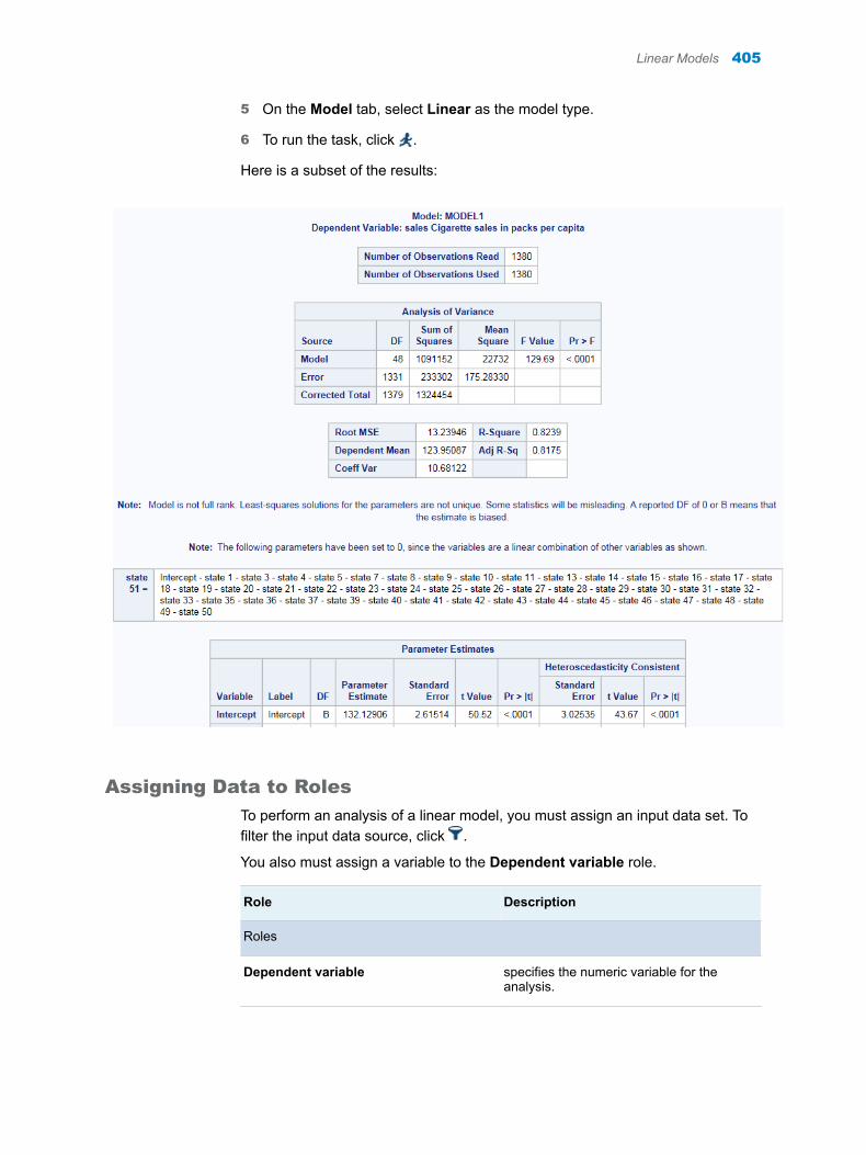
5 On the Model tab, select Linear as the model type.
6 To run the task, click .
Here is a subset of the results:
Assigning Data to Roles
To perform an analysis of a linear model, you must assign an input data set. To filter the input data source, click .
You also must assign a variable to the Dependent variable role.
Role Description
Roles
Dependent variable specifies the numeric variable for the analysis.
Linear Models 405
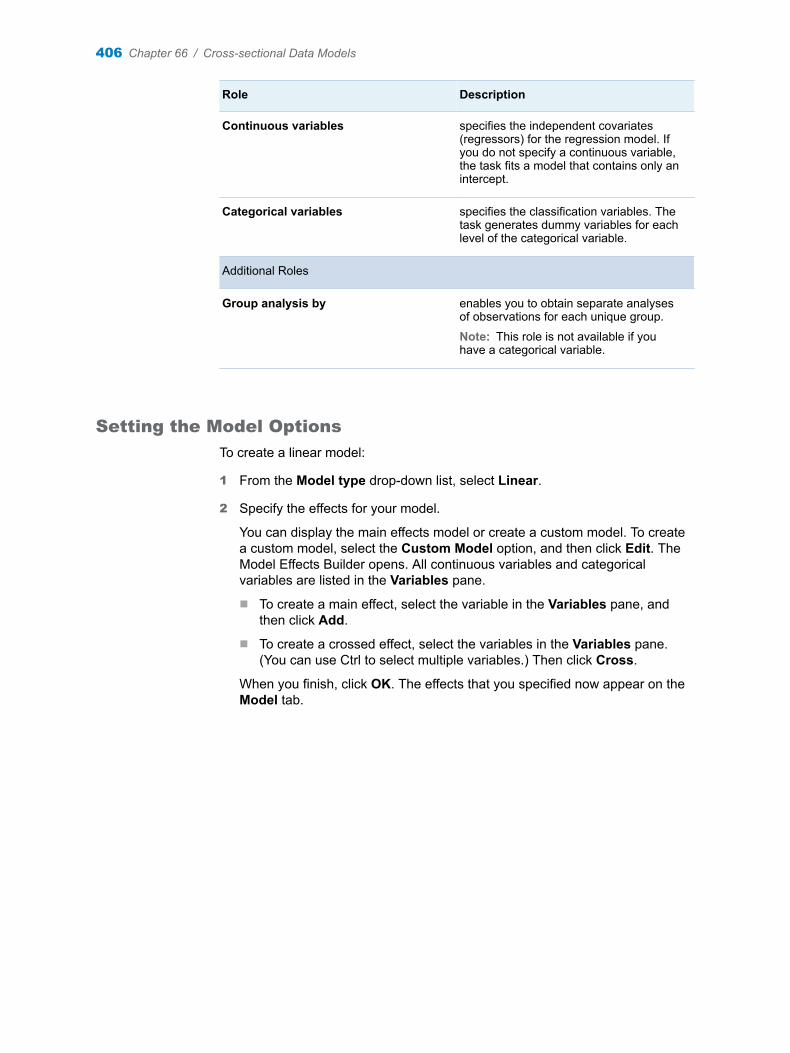
Role Description
Continuous variables specifies the independent covariates (regressors) for the regression model. If you do not specify a continuous variable, the task fits a model that contains only an intercept.
Categorical variables specifies the classification variables. The task generates dummy variables for each level of the categorical variable.
Additional Roles
Group analysis by enables you to obtain separate analyses of observations for each unique group.
Note: This role is not available if you have a categorical variable.
Setting the Model Options
To create a linear model:
1 From the Model type drop-down list, select Linear.
2 Specify the effects for your model.
You can display the main effects model or create a custom model. To create a custom model, select the Custom Model option, and then click Edit. The Model Effects Builder opens. All continuous variables and categorical variables are listed in the Variables pane.
n To create a main effect, select the variable in the Variables pane, and then click Add.
n To create a crossed effect, select the variables in the Variables pane. (You can use Ctrl to select multiple variables.) Then click Cross.
When you finish, click OK. The effects that you specified now appear on the Model tab.
406 Chapter 66 / Cross-sectional Data Models

Here is an example of model effects on the Model tab.
Setting the Options
Option Name Description
Methods
Covariance matrix estimator
specifies the method to calculate the covariance matrix of parameter estimates.
You can select the default value, or you can choose from these methods:
n Whiten HCn specifies a heteroscedasticity-corrected covariance
matrix. n is a value from 0–3.
Statistics
Select the statistics to display in the results.
Here are the additional statistics that you can include in the results:
n correlations of the parameter estimatesn covariances of the parameter estimatesn heteroscedasticity-consistent standard errors
Plots
Linear Models 407

Option Name Description
Select the plots to include in the results. By default, diagnostic, residual, and fit plots are included in the results. You can include these plots:n diagnostic plots, such as residuals for each explanatory variable, R-student statistic
by predicted values, and normal quantile plot of the residualsn output plots, such as a fit plot for a single continuous variable, a plot of observed
values by predicted values, and partial regression plots for each explanatory variable
You can choose to display these plots as a panel of plots or as individual plots.
Creating the Output Data Sets
You can create an output data set that contains the parameter estimates.
Logit Model
Example: Logit Model
To create this example:
1 Create the Work.Moz data set. For more information, see “MROZ Data Set” on page 608.
2 In the Tasks section, expand the Econometrics folder, and then double-click Cross-sectional Data Models. The user interface for the Cross-Sectional Data Models task opens.
3 On the Data tab, select the WORK.MROZ data set.
TIP If the data set is not available from the drop-down list, click . In
the Choose a Table window, expand the library that contains the data set that you want to use. Select the data set for the example and click OK. The selected data set should now appear in the drop-down list.
4 Assign columns to these roles:
Role Column Name
Dependent variable inlf
Continuous variables nwifeinceducexperexpersq
Categorical variables kidsge6
408 Chapter 66 / Cross-sectional Data Models
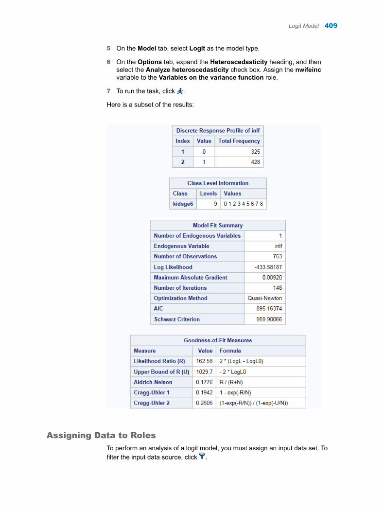
5 On the Model tab, select Logit as the model type.
6 On the Options tab, expand the Heteroscedasticity heading, and then select the Analyze heteroscedasticity check box. Assign the nwifeinc variable to the Variables on the variance function role.
7 To run the task, click .
Here is a subset of the results:
Assigning Data to Roles
To perform an analysis of a logit model, you must assign an input data set. To filter the input data source, click .
Logit Model 409
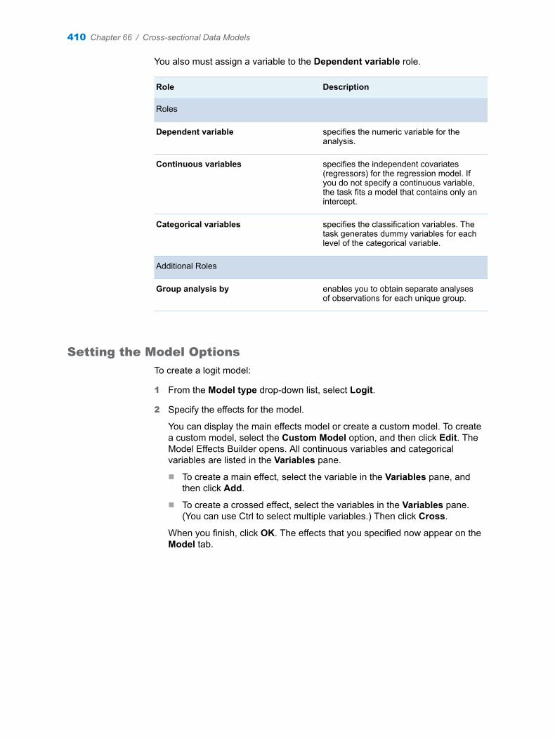
You also must assign a variable to the Dependent variable role.
Role Description
Roles
Dependent variable specifies the numeric variable for the analysis.
Continuous variables specifies the independent covariates (regressors) for the regression model. If you do not specify a continuous variable, the task fits a model that contains only an intercept.
Categorical variables specifies the classification variables. The task generates dummy variables for each level of the categorical variable.
Additional Roles
Group analysis by enables you to obtain separate analyses of observations for each unique group.
Setting the Model Options
To create a logit model:
1 From the Model type drop-down list, select Logit.
2 Specify the effects for the model.
You can display the main effects model or create a custom model. To create a custom model, select the Custom Model option, and then click Edit. The Model Effects Builder opens. All continuous variables and categorical variables are listed in the Variables pane.
n To create a main effect, select the variable in the Variables pane, and then click Add.
n To create a crossed effect, select the variables in the Variables pane. (You can use Ctrl to select multiple variables.) Then click Cross.
When you finish, click OK. The effects that you specified now appear on the Model tab.
410 Chapter 66 / Cross-sectional Data Models
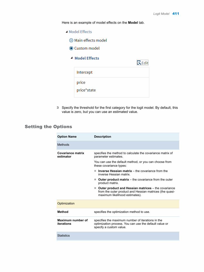
Here is an example of model effects on the Model tab.
3 Specify the threshold for the first category for the logit model. By default, this value is zero, but you can use an estimated value.
Setting the Options
Option Name Description
Methods
Covariance matrix estimator
specifies the method to calculate the covariance matrix of parameter estimates.
You can use the default method, or you can choose from these covariance types:
n Inverse Hessian matrix – the covariance from the inverse Hessian matrix.
n Outer product matrix – the covariance from the outer product matrix.
n Outer product and Hessian matrices – the covariance from the outer product and Hessian matrices (the quasi-maximum likelihood estimates).
Optimization
Method specifies the optimization method to use.
Maximum number of iterations
specifies the maximum number of iterations in the optimization process. You can use the default value or specify a custom value.
Statistics
Logit Model 411
Option Name Description
Select the statistics to display in the results.
Here are the additional statistics that you can include in the results:
n correlations of the parameter estimatesn covariances of the parameter estimatesn iteration history of the objective function and parameter estimates
Plots
You can choose to display only the default plots, the selected plots, or no plots in the results.
You can choose from these types of plots:
n diagnostic plots, such as error standard deviations by observed regressor and profiled log likelihood
n output plots, such as predicted values by regressor, marginal effects by regressor, Inverse Mills ratio by regressor, predicted response probability by regressor, predicted probabilities for each level of the response by regressor, and linear predictor values by regressor
Creating the Output Data Sets
You can create these output data sets:
n an output data set that contains the default statistics from the analysis and additional statistics, such as predicted values, the probability of the dependent variable taking the current value, the probability of the dependent variable for all possible responses, and the error standard deviation
n a parameter estimates data set
Probit Model
Example: Probit Model
To create this example:
1 Create the Work.Moz data set. For more information, see “MROZ Data Set” on page 608.
2 In the Tasks section, expand the Econometrics folder, and then double-click Cross-sectional Data Models. The user interface for the Cross-Sectional Data Models task opens.
3 On the Data tab, select the WORK.MROZ data set.
TIP If the data set is not available from the drop-down list, click . In
the Choose a Table window, expand the library that contains the data set
412 Chapter 66 / Cross-sectional Data Models
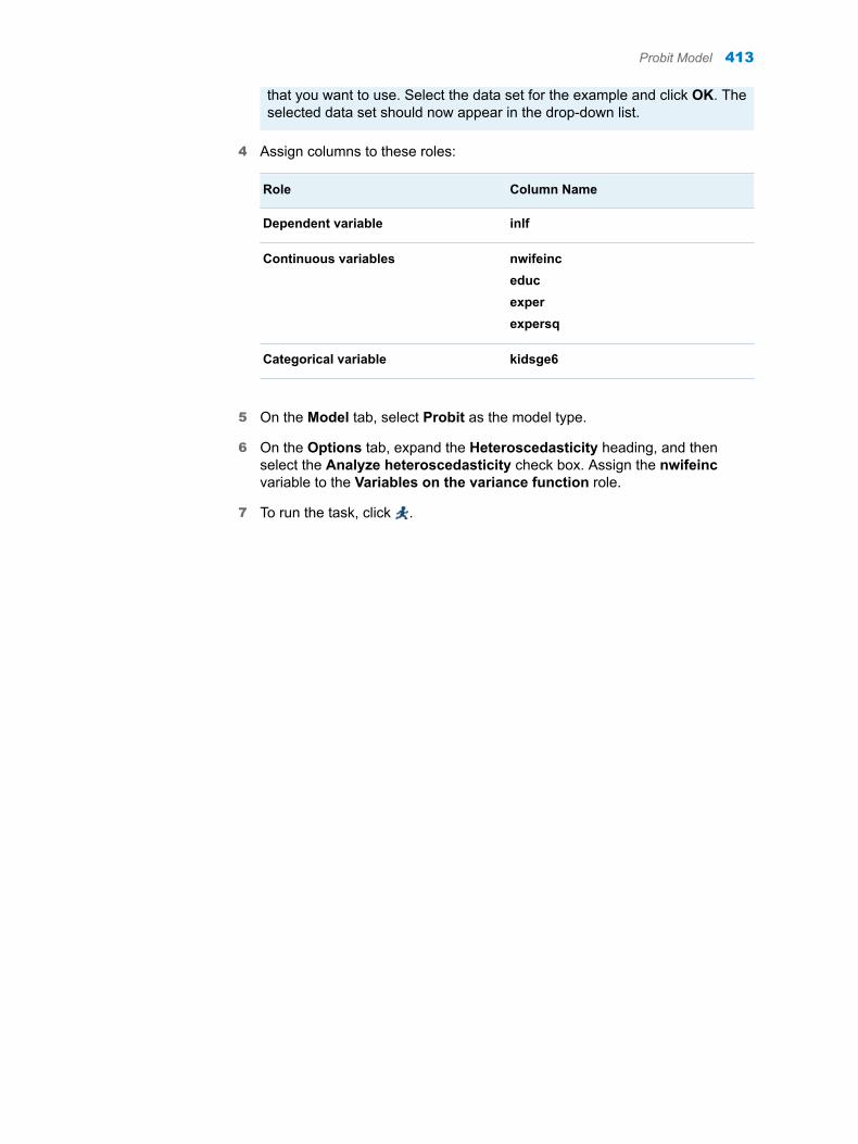
that you want to use. Select the data set for the example and click OK. The selected data set should now appear in the drop-down list.
4 Assign columns to these roles:
Role Column Name
Dependent variable inlf
Continuous variables nwifeinceducexperexpersq
Categorical variable kidsge6
5 On the Model tab, select Probit as the model type.
6 On the Options tab, expand the Heteroscedasticity heading, and then select the Analyze heteroscedasticity check box. Assign the nwifeinc variable to the Variables on the variance function role.
7 To run the task, click .
Probit Model 413

Here is a subset of the results:
Assigning Data to Roles
To perform an analysis of a probit model, you must assign an input data set. To filter the input data source, click .
You also must assign a variable to the Dependent variable role.
Role Description
Roles
Dependent variable specifies the numeric variable for the analysis.
414 Chapter 66 / Cross-sectional Data Models
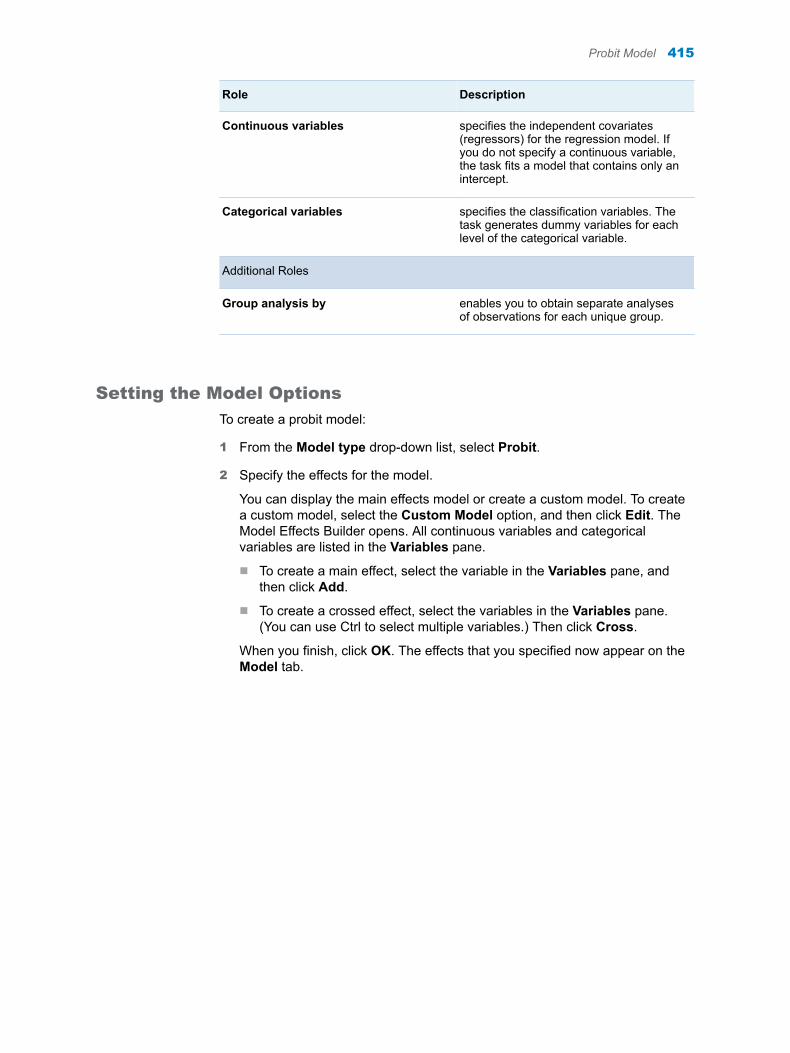
Role Description
Continuous variables specifies the independent covariates (regressors) for the regression model. If you do not specify a continuous variable, the task fits a model that contains only an intercept.
Categorical variables specifies the classification variables. The task generates dummy variables for each level of the categorical variable.
Additional Roles
Group analysis by enables you to obtain separate analyses of observations for each unique group.
Setting the Model Options
To create a probit model:
1 From the Model type drop-down list, select Probit.
2 Specify the effects for the model.
You can display the main effects model or create a custom model. To create a custom model, select the Custom Model option, and then click Edit. The Model Effects Builder opens. All continuous variables and categorical variables are listed in the Variables pane.
n To create a main effect, select the variable in the Variables pane, and then click Add.
n To create a crossed effect, select the variables in the Variables pane. (You can use Ctrl to select multiple variables.) Then click Cross.
When you finish, click OK. The effects that you specified now appear on the Model tab.
Probit Model 415
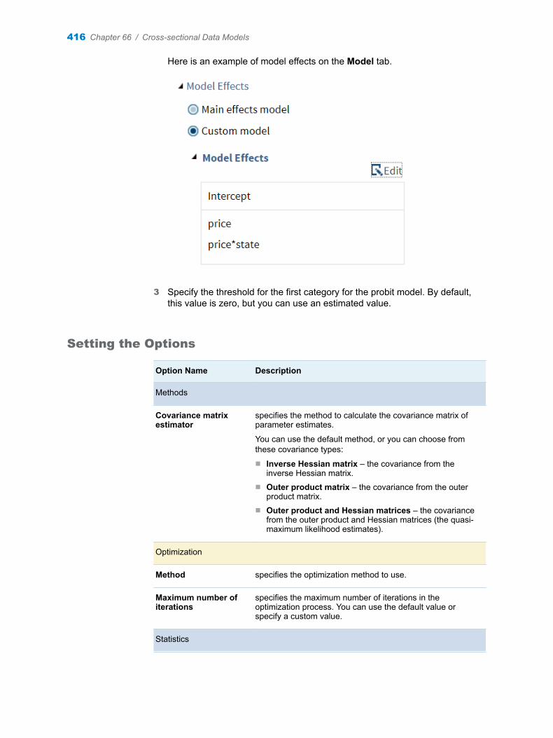
Here is an example of model effects on the Model tab.
3 Specify the threshold for the first category for the probit model. By default, this value is zero, but you can use an estimated value.
Setting the Options
Option Name Description
Methods
Covariance matrix estimator
specifies the method to calculate the covariance matrix of parameter estimates.
You can use the default method, or you can choose from these covariance types:
n Inverse Hessian matrix – the covariance from the inverse Hessian matrix.
n Outer product matrix – the covariance from the outer product matrix.
n Outer product and Hessian matrices – the covariance from the outer product and Hessian matrices (the quasi-maximum likelihood estimates).
Optimization
Method specifies the optimization method to use.
Maximum number of iterations
specifies the maximum number of iterations in the optimization process. You can use the default value or specify a custom value.
Statistics
416 Chapter 66 / Cross-sectional Data Models
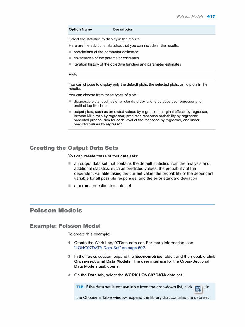
Option Name Description
Select the statistics to display in the results.
Here are the additional statistics that you can include in the results:
n correlations of the parameter estimatesn covariances of the parameter estimatesn iteration history of the objective function and parameter estimates
Plots
You can choose to display only the default plots, the selected plots, or no plots in the results.
You can choose from these types of plots:
n diagnostic plots, such as error standard deviations by observed regressor and profiled log likelihood
n output plots, such as predicted values by regressor, marginal effects by regressor, Inverse Mills ratio by regressor, predicted response probability by regressor, predicted probabilities for each level of the response by regressor, and linear predictor values by regressor
Creating the Output Data Sets
You can create these output data sets:
n an output data set that contains the default statistics from the analysis and additional statistics, such as predicted values, the probability of the dependent variable taking the current value, the probability of the dependent variable for all possible responses, and the error standard deviation
n a parameter estimates data set
Poisson Models
Example: Poisson Model
To create this example:
1 Create the Work.Long97Data data set. For more information, see “LONG97DATA Data Set” on page 592.
2 In the Tasks section, expand the Econometrics folder, and then double-click Cross-sectional Data Models. The user interface for the Cross-Sectional Data Models task opens.
3 On the Data tab, select the WORK.LONG97DATA data set.
TIP If the data set is not available from the drop-down list, click . In
the Choose a Table window, expand the library that contains the data set
Poisson Models 417
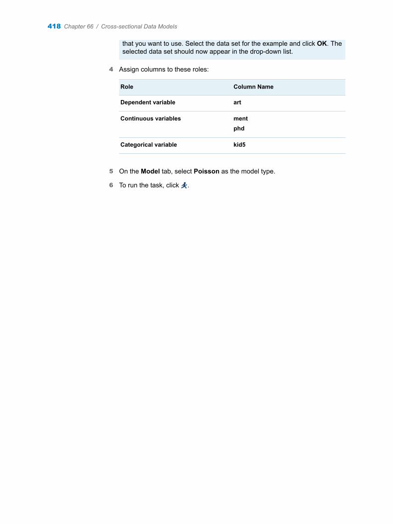
that you want to use. Select the data set for the example and click OK. The selected data set should now appear in the drop-down list.
4 Assign columns to these roles:
Role Column Name
Dependent variable art
Continuous variables mentphd
Categorical variable kid5
5 On the Model tab, select Poisson as the model type.
6 To run the task, click .
418 Chapter 66 / Cross-sectional Data Models
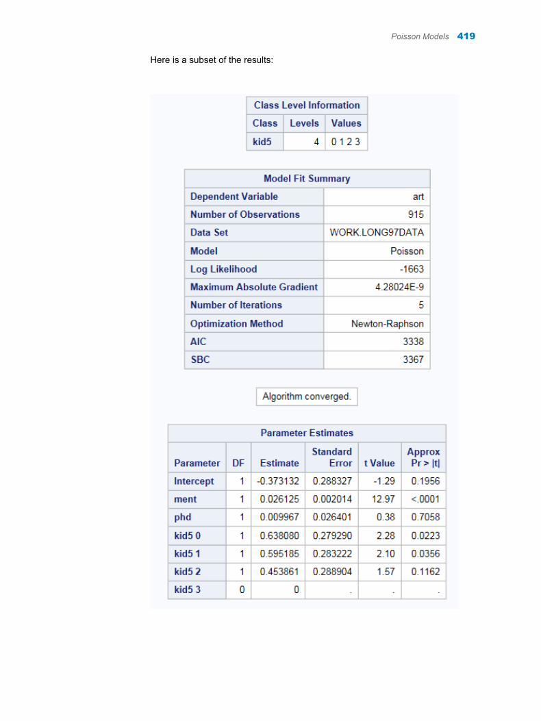
Here is a subset of the results:
Poisson Models 419
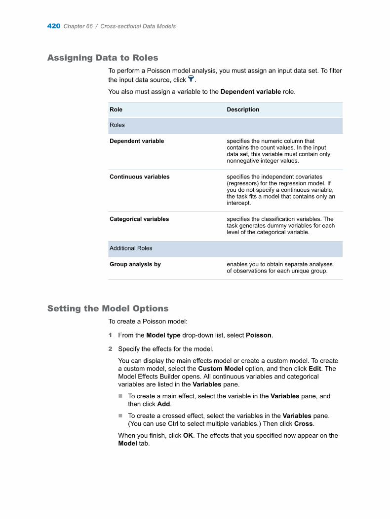
Assigning Data to Roles
To perform a Poisson model analysis, you must assign an input data set. To filter the input data source, click .
You also must assign a variable to the Dependent variable role.
Role Description
Roles
Dependent variable specifies the numeric column that contains the count values. In the input data set, this variable must contain only nonnegative integer values.
Continuous variables specifies the independent covariates (regressors) for the regression model. If you do not specify a continuous variable, the task fits a model that contains only an intercept.
Categorical variables specifies the classification variables. The task generates dummy variables for each level of the categorical variable.
Additional Roles
Group analysis by enables you to obtain separate analyses of observations for each unique group.
Setting the Model Options
To create a Poisson model:
1 From the Model type drop-down list, select Poisson.
2 Specify the effects for the model.
You can display the main effects model or create a custom model. To create a custom model, select the Custom Model option, and then click Edit. The Model Effects Builder opens. All continuous variables and categorical variables are listed in the Variables pane.
n To create a main effect, select the variable in the Variables pane, and then click Add.
n To create a crossed effect, select the variables in the Variables pane. (You can use Ctrl to select multiple variables.) Then click Cross.
When you finish, click OK. The effects that you specified now appear on the Model tab.
420 Chapter 66 / Cross-sectional Data Models

Here is an example of model effects on the Model tab.
Setting the Options
Option Name Description
Methods
Covariance matrix estimator
specifies the method to calculate the covariance matrix of parameter estimates.
You can use the default value, or you can choose from these covariance types:
n Inverse Hessian matrix –the covariance from the inverse Hessian matrix.
n Outer product matrix – the covariance from the outer product matrix.
n Outer product and Hessian matrices – the covariance from the outer product and Hessian matrices (the quasi-maximum likelihood estimates).
Optimization
Method specifies the optimization method to use.
Maximum number of iterations
specifies the maximum number of iterations in the optimization process. You can use the default value, or you can specify a custom value.
Statistics
Poisson Models 421
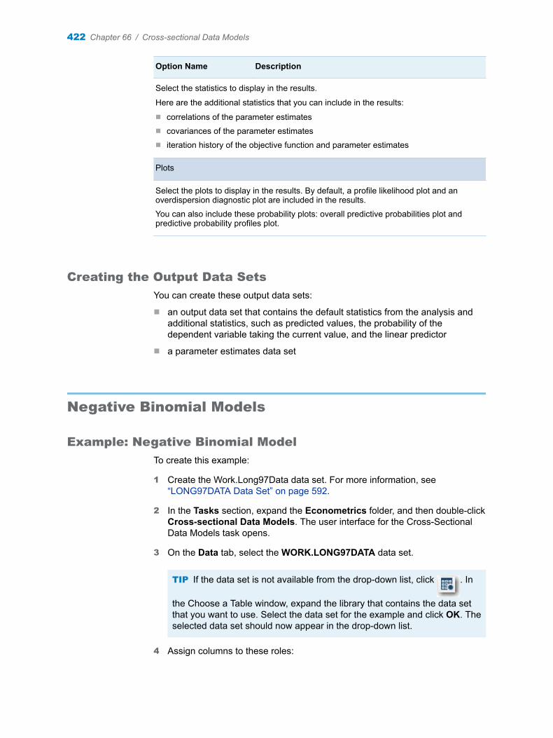
Option Name Description
Select the statistics to display in the results.
Here are the additional statistics that you can include in the results:
n correlations of the parameter estimatesn covariances of the parameter estimatesn iteration history of the objective function and parameter estimates
Plots
Select the plots to display in the results. By default, a profile likelihood plot and an overdispersion diagnostic plot are included in the results.
You can also include these probability plots: overall predictive probabilities plot and predictive probability profiles plot.
Creating the Output Data Sets
You can create these output data sets:
n an output data set that contains the default statistics from the analysis and additional statistics, such as predicted values, the probability of the dependent variable taking the current value, and the linear predictor
n a parameter estimates data set
Negative Binomial Models
Example: Negative Binomial Model
To create this example:
1 Create the Work.Long97Data data set. For more information, see “LONG97DATA Data Set” on page 592.
2 In the Tasks section, expand the Econometrics folder, and then double-click Cross-sectional Data Models. The user interface for the Cross-Sectional Data Models task opens.
3 On the Data tab, select the WORK.LONG97DATA data set.
TIP If the data set is not available from the drop-down list, click . In
the Choose a Table window, expand the library that contains the data set that you want to use. Select the data set for the example and click OK. The selected data set should now appear in the drop-down list.
4 Assign columns to these roles:
422 Chapter 66 / Cross-sectional Data Models

Role Column Name
Dependent variable art
Continuous variables mentphd
Categorical variable kid5
5 On the Model tab, select Negative binomial as the model type.
6 To run the task, click .
Here is a subset of the results:
Negative Binomial Models 423
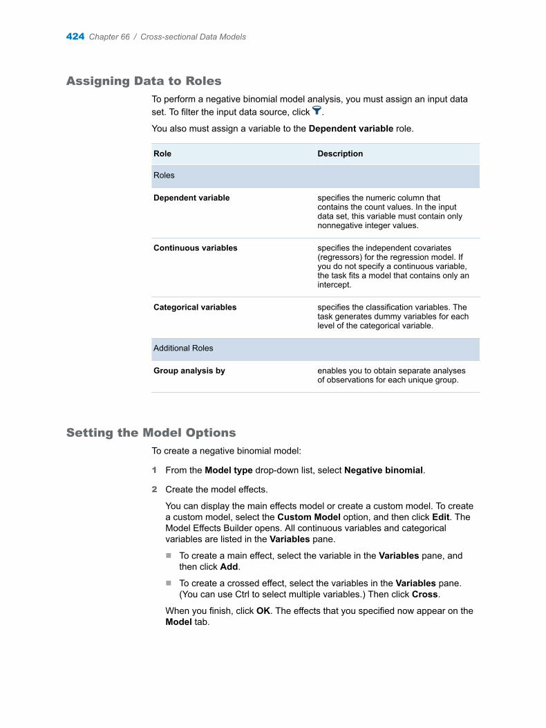
Assigning Data to Roles
To perform a negative binomial model analysis, you must assign an input data set. To filter the input data source, click .
You also must assign a variable to the Dependent variable role.
Role Description
Roles
Dependent variable specifies the numeric column that contains the count values. In the input data set, this variable must contain only nonnegative integer values.
Continuous variables specifies the independent covariates (regressors) for the regression model. If you do not specify a continuous variable, the task fits a model that contains only an intercept.
Categorical variables specifies the classification variables. The task generates dummy variables for each level of the categorical variable.
Additional Roles
Group analysis by enables you to obtain separate analyses of observations for each unique group.
Setting the Model Options
To create a negative binomial model:
1 From the Model type drop-down list, select Negative binomial.
2 Create the model effects.
You can display the main effects model or create a custom model. To create a custom model, select the Custom Model option, and then click Edit. The Model Effects Builder opens. All continuous variables and categorical variables are listed in the Variables pane.
n To create a main effect, select the variable in the Variables pane, and then click Add.
n To create a crossed effect, select the variables in the Variables pane. (You can use Ctrl to select multiple variables.) Then click Cross.
When you finish, click OK. The effects that you specified now appear on the Model tab.
424 Chapter 66 / Cross-sectional Data Models
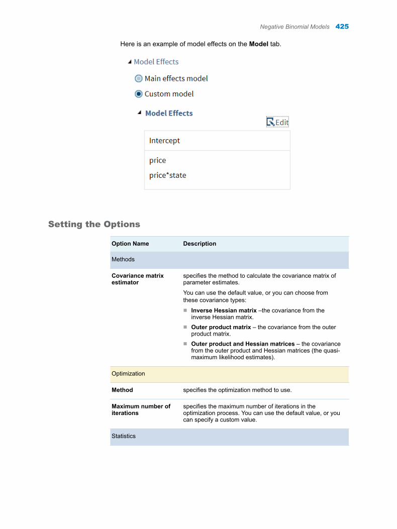
Here is an example of model effects on the Model tab.
Setting the Options
Option Name Description
Methods
Covariance matrix estimator
specifies the method to calculate the covariance matrix of parameter estimates.
You can use the default value, or you can choose from these covariance types:
n Inverse Hessian matrix –the covariance from the inverse Hessian matrix.
n Outer product matrix – the covariance from the outer product matrix.
n Outer product and Hessian matrices – the covariance from the outer product and Hessian matrices (the quasi-maximum likelihood estimates).
Optimization
Method specifies the optimization method to use.
Maximum number of iterations
specifies the maximum number of iterations in the optimization process. You can use the default value, or you can specify a custom value.
Statistics
Negative Binomial Models 425
Option Name Description
Select the statistics to display in the results.
Here are the additional statistics that you can include in the results:
n correlations of the parameter estimatesn covariances of the parameter estimatesn iteration history of the objective function and parameter estimates
Plots
Select the plots to display in the results. By default, a profile likelihood plot and an overdispersion diagnostic plot are included in the results.
You can also include these probability plots: overall predictive probabilities plot and predictive probability profiles plot.
Creating the Output Data Sets
You can create these output data sets:
n an output data set that contains the default statistics from the analysis and additional statistics, such as predicted values, the probability of the dependent variable taking the current value, and the linear predictor
n a parameter estimates data set
Censored Regression
Example: Censored Regression
To create this example:
1 Create the Work.Cigar data set. For more information, see “CIGAR Data Set” on page 563.
2 In the Tasks section, expand the Econometrics folder, and then double-click Cross-sectional Data Models. The user interface for the Cross-Sectional Data Models task opens.
3 On the Data tab, select the WORK.CIGAR data set.
TIP If the data set is not available from the drop-down list, click . In
the Choose a Table window, expand the library that contains the data set that you want to use. Select the data set for the example and click OK. The selected data set should now appear in the drop-down list.
4 Assign columns to these roles:
426 Chapter 66 / Cross-sectional Data Models
Role Column Name
Dependent variable sales
Continuous variables pricecpindi
Categorical variables state
5 On the Model tab, complete these steps:
a Select Censored regression as the model type.
b Select the Set the lower bound check box. From the Lower bound method drop-down list, select Specify by value. In the Lower bound value box, enter 90.
6 On the Options tab, expand the Heteroscedasticity heading, and then select the Analyze heteroscedasticity check box. Assign the price variable to the Variables on the variance function role.
7 To run the task, click .
Censored Regression 427
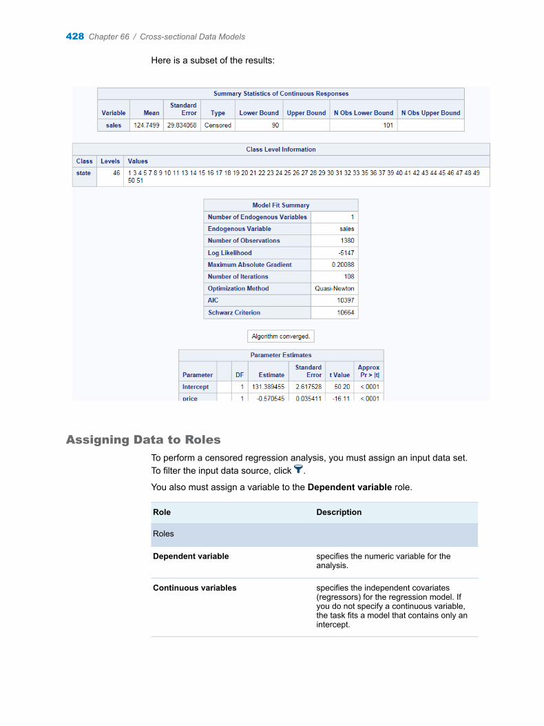
Here is a subset of the results:
Assigning Data to Roles
To perform a censored regression analysis, you must assign an input data set. To filter the input data source, click .
You also must assign a variable to the Dependent variable role.
Role Description
Roles
Dependent variable specifies the numeric variable for the analysis.
Continuous variables specifies the independent covariates (regressors) for the regression model. If you do not specify a continuous variable, the task fits a model that contains only an intercept.
428 Chapter 66 / Cross-sectional Data Models
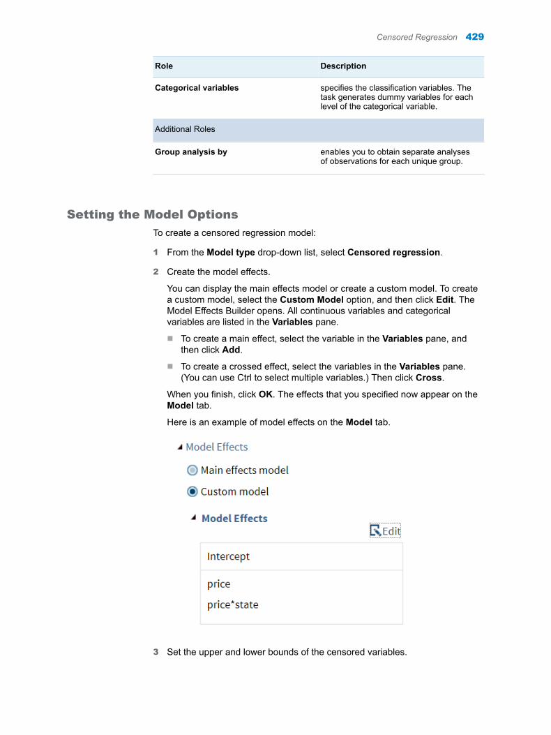
Role Description
Categorical variables specifies the classification variables. The task generates dummy variables for each level of the categorical variable.
Additional Roles
Group analysis by enables you to obtain separate analyses of observations for each unique group.
Setting the Model Options
To create a censored regression model:
1 From the Model type drop-down list, select Censored regression.
2 Create the model effects.
You can display the main effects model or create a custom model. To create a custom model, select the Custom Model option, and then click Edit. The Model Effects Builder opens. All continuous variables and categorical variables are listed in the Variables pane.
n To create a main effect, select the variable in the Variables pane, and then click Add.
n To create a crossed effect, select the variables in the Variables pane. (You can use Ctrl to select multiple variables.) Then click Cross.
When you finish, click OK. The effects that you specified now appear on the Model tab.
Here is an example of model effects on the Model tab.
3 Set the upper and lower bounds of the censored variables.
Censored Regression 429

Note: If you do not specify an upper bound or a lower bound, the result is a linear regression model.
Setting the Options
Option Name Description
Methods
Covariance matrix estimator
specifies the method to calculate the covariance matrix of parameter estimates.
You can use the default value, or you can choose from these covariance types:
n Inverse Hessian matrix – the covariance from the inverse Hessian matrix.
n Outer product matrix – the covariance from the outer product matrix.
n Outer product and Hessian matrices – the covariance from the outer product and Hessian matrices (the quasi-maximum likelihood estimates).
Optimization
Method specifies the optimization method to use.
Maximum number of iterations
specifies the maximum number of iterations in the optimization process. You can use the default value, or you can specify a custom value.
Statistics
Select the statistics to display in the results.
Here are the additional statistics that you can include in the results:
n correlations of the parameter estimatesn covariances of the parameter estimatesn iteration history of the objective function and parameter estimates
Creating the Output Data Sets
You can create these output data sets:
n an output data set that contains the default statistics from the analysis and additional statistics, such as predicted values, residuals, error standard deviation, linear predictor, and so on.
n a parameter estimates data set
430 Chapter 66 / Cross-sectional Data Models

Truncated Regression
Example: Truncated Regression
To create this example:
1 Create the Work.Cigar data set. For more information, see “CIGAR Data Set” on page 563.
2 In the Tasks section, expand the Econometrics folder, and then double-click Cross-sectional Data Models. The user interface for the Cross-Sectional Data Models task opens.
3 On the Data tab, select the WORK.CIGAR data set.
TIP If the data set is not available from the drop-down list, click . In
the Choose a Table window, expand the library that contains the data set that you want to use. Select the data set for the example and click OK. The selected data set should now appear in the drop-down list.
4 Assign columns to these roles:
Role Column Name
Dependent variable sales
Continuous variables pricecpindi
Categorical variables state
5 On the Model tab, complete these steps:
a Select Truncated regression as the model type.
b Select the Set the lower bound check box. From the Lower bound method drop-down list, select Specify by value. In the Lower bound value box, enter 90.
6 On the Options tab, expand the Heteroscedasticity heading, and then select the Analyze heteroscedasticity check box. Assign the price variable to the Variables on the variance function role.
7 To run the task, click .
Truncated Regression 431
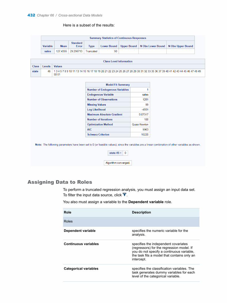
Here is a subset of the results:
Assigning Data to Roles
To perform a truncated regression analysis, you must assign an input data set. To filter the input data source, click .
You also must assign a variable to the Dependent variable role.
Role Description
Roles
Dependent variable specifies the numeric variable for the analysis.
Continuous variables specifies the independent covariates (regressors) for the regression model. If you do not specify a continuous variable, the task fits a model that contains only an intercept.
Categorical variables specifies the classification variables. The task generates dummy variables for each level of the categorical variable.
432 Chapter 66 / Cross-sectional Data Models
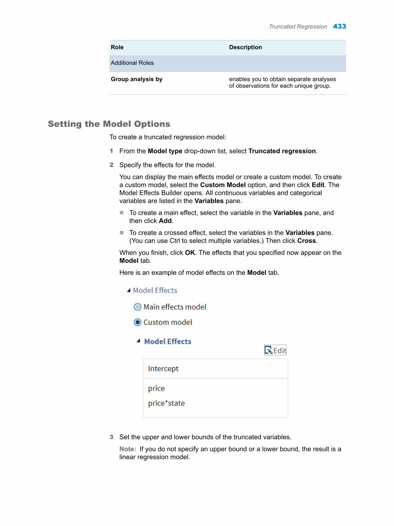
Role Description
Additional Roles
Group analysis by enables you to obtain separate analyses of observations for each unique group.
Setting the Model Options
To create a truncated regression model:
1 From the Model type drop-down list, select Truncated regression.
2 Specify the effects for the model.
You can display the main effects model or create a custom model. To create a custom model, select the Custom Model option, and then click Edit. The Model Effects Builder opens. All continuous variables and categorical variables are listed in the Variables pane.
n To create a main effect, select the variable in the Variables pane, and then click Add.
n To create a crossed effect, select the variables in the Variables pane. (You can use Ctrl to select multiple variables.) Then click Cross.
When you finish, click OK. The effects that you specified now appear on the Model tab.
Here is an example of model effects on the Model tab.
3 Set the upper and lower bounds of the truncated variables.
Note: If you do not specify an upper bound or a lower bound, the result is a linear regression model.
Truncated Regression 433
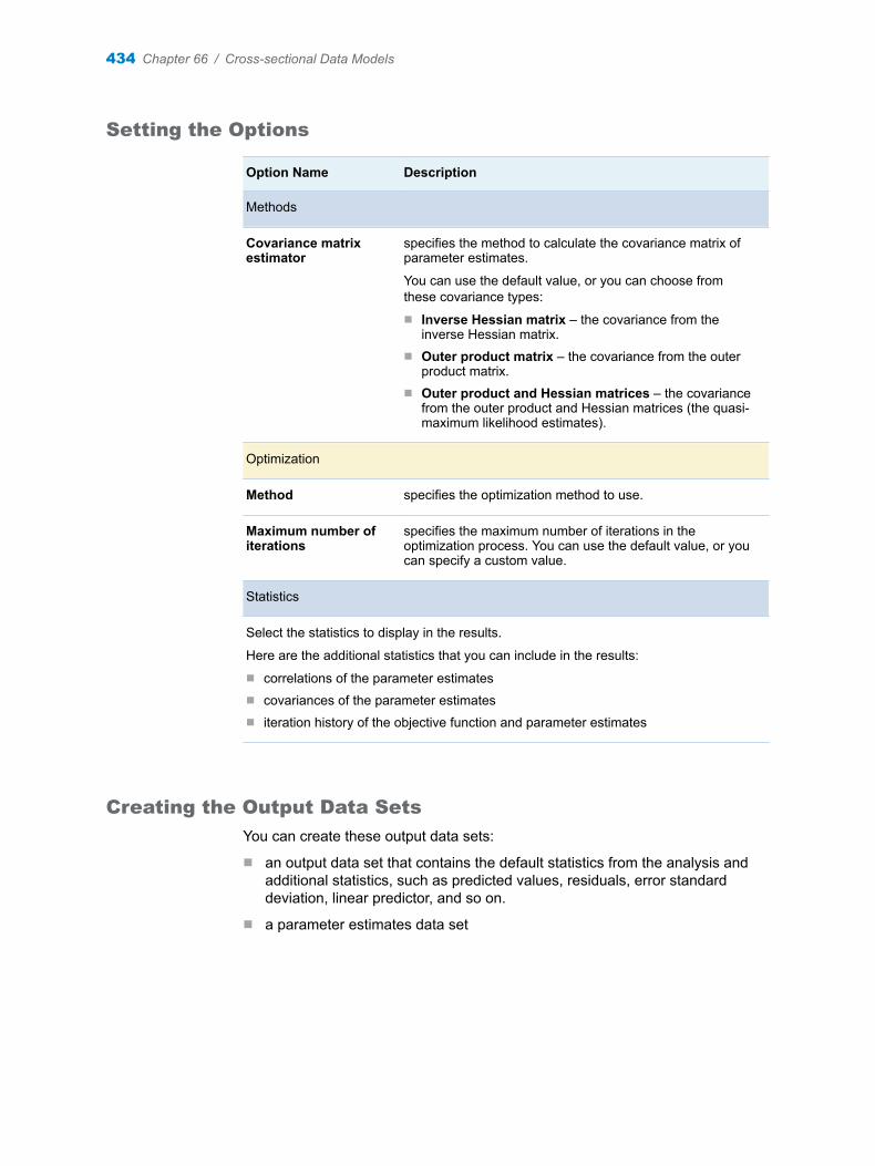
Setting the Options
Option Name Description
Methods
Covariance matrix estimator
specifies the method to calculate the covariance matrix of parameter estimates.
You can use the default value, or you can choose from these covariance types:
n Inverse Hessian matrix – the covariance from the inverse Hessian matrix.
n Outer product matrix – the covariance from the outer product matrix.
n Outer product and Hessian matrices – the covariance from the outer product and Hessian matrices (the quasi-maximum likelihood estimates).
Optimization
Method specifies the optimization method to use.
Maximum number of iterations
specifies the maximum number of iterations in the optimization process. You can use the default value, or you can specify a custom value.
Statistics
Select the statistics to display in the results.
Here are the additional statistics that you can include in the results:
n correlations of the parameter estimatesn covariances of the parameter estimatesn iteration history of the objective function and parameter estimates
Creating the Output Data Sets
You can create these output data sets:
n an output data set that contains the default statistics from the analysis and additional statistics, such as predicted values, residuals, error standard deviation, linear predictor, and so on.
n a parameter estimates data set
434 Chapter 66 / Cross-sectional Data Models
67Panel Data Models
About the Panel Data Models Task . . . . . . . . . . . . . . . . . . . . . . . . . . . . . . . . . . . . . . . . . 436
Linear Models . . . . . . . . . . . . . . . . . . . . . . . . . . . . . . . . . . . . . . . . . . . . . . . . . . . . . . . . . . . . . 436Example: Linear Regression with Fixed Effects . . . . . . . . . . . . . . . . . . . . . . . . . . . . 436Assigning Data to Roles . . . . . . . . . . . . . . . . . . . . . . . . . . . . . . . . . . . . . . . . . . . . . . . . . 437Setting the Model Options . . . . . . . . . . . . . . . . . . . . . . . . . . . . . . . . . . . . . . . . . . . . . . . 438Setting the Options . . . . . . . . . . . . . . . . . . . . . . . . . . . . . . . . . . . . . . . . . . . . . . . . . . . . . . 439Creating the Output Data Sets . . . . . . . . . . . . . . . . . . . . . . . . . . . . . . . . . . . . . . . . . . . 440
Logit Model . . . . . . . . . . . . . . . . . . . . . . . . . . . . . . . . . . . . . . . . . . . . . . . . . . . . . . . . . . . . . . . 441Example: Logit Model . . . . . . . . . . . . . . . . . . . . . . . . . . . . . . . . . . . . . . . . . . . . . . . . . . . . 441Assigning Data to Roles . . . . . . . . . . . . . . . . . . . . . . . . . . . . . . . . . . . . . . . . . . . . . . . . . 442Setting the Model Options . . . . . . . . . . . . . . . . . . . . . . . . . . . . . . . . . . . . . . . . . . . . . . . 443Setting the Options . . . . . . . . . . . . . . . . . . . . . . . . . . . . . . . . . . . . . . . . . . . . . . . . . . . . . . 444Creating the Output Data Sets . . . . . . . . . . . . . . . . . . . . . . . . . . . . . . . . . . . . . . . . . . . 445
Probit Model . . . . . . . . . . . . . . . . . . . . . . . . . . . . . . . . . . . . . . . . . . . . . . . . . . . . . . . . . . . . . . . 445Example: Probit Model . . . . . . . . . . . . . . . . . . . . . . . . . . . . . . . . . . . . . . . . . . . . . . . . . . . 445Assigning Data to Roles . . . . . . . . . . . . . . . . . . . . . . . . . . . . . . . . . . . . . . . . . . . . . . . . . 447Setting the Model Options . . . . . . . . . . . . . . . . . . . . . . . . . . . . . . . . . . . . . . . . . . . . . . . 448Setting the Options . . . . . . . . . . . . . . . . . . . . . . . . . . . . . . . . . . . . . . . . . . . . . . . . . . . . . . 449Creating the Output Data Sets . . . . . . . . . . . . . . . . . . . . . . . . . . . . . . . . . . . . . . . . . . . 450
Poisson Models . . . . . . . . . . . . . . . . . . . . . . . . . . . . . . . . . . . . . . . . . . . . . . . . . . . . . . . . . . . 450Example: Poisson Model . . . . . . . . . . . . . . . . . . . . . . . . . . . . . . . . . . . . . . . . . . . . . . . . . 450Assigning Data to Roles . . . . . . . . . . . . . . . . . . . . . . . . . . . . . . . . . . . . . . . . . . . . . . . . . 452Setting the Model Options . . . . . . . . . . . . . . . . . . . . . . . . . . . . . . . . . . . . . . . . . . . . . . . 453Setting the Options . . . . . . . . . . . . . . . . . . . . . . . . . . . . . . . . . . . . . . . . . . . . . . . . . . . . . . 454Creating the Output Data Sets . . . . . . . . . . . . . . . . . . . . . . . . . . . . . . . . . . . . . . . . . . . 454
Negative Binomial Models . . . . . . . . . . . . . . . . . . . . . . . . . . . . . . . . . . . . . . . . . . . . . . . . . 455Example: Negative Binomial Model . . . . . . . . . . . . . . . . . . . . . . . . . . . . . . . . . . . . . . . 455Assigning Data to Roles . . . . . . . . . . . . . . . . . . . . . . . . . . . . . . . . . . . . . . . . . . . . . . . . . 456Setting the Model Options . . . . . . . . . . . . . . . . . . . . . . . . . . . . . . . . . . . . . . . . . . . . . . . 457Setting the Options . . . . . . . . . . . . . . . . . . . . . . . . . . . . . . . . . . . . . . . . . . . . . . . . . . . . . . 458Creating the Output Data Sets . . . . . . . . . . . . . . . . . . . . . . . . . . . . . . . . . . . . . . . . . . . 459
Censored Regression . . . . . . . . . . . . . . . . . . . . . . . . . . . . . . . . . . . . . . . . . . . . . . . . . . . . . 459Example: Censored Regression . . . . . . . . . . . . . . . . . . . . . . . . . . . . . . . . . . . . . . . . . . 459Assigning Data to Roles . . . . . . . . . . . . . . . . . . . . . . . . . . . . . . . . . . . . . . . . . . . . . . . . . 460Setting the Model Options . . . . . . . . . . . . . . . . . . . . . . . . . . . . . . . . . . . . . . . . . . . . . . . 461Setting the Options . . . . . . . . . . . . . . . . . . . . . . . . . . . . . . . . . . . . . . . . . . . . . . . . . . . . . . 462Creating the Output Data Sets . . . . . . . . . . . . . . . . . . . . . . . . . . . . . . . . . . . . . . . . . . . 463
435
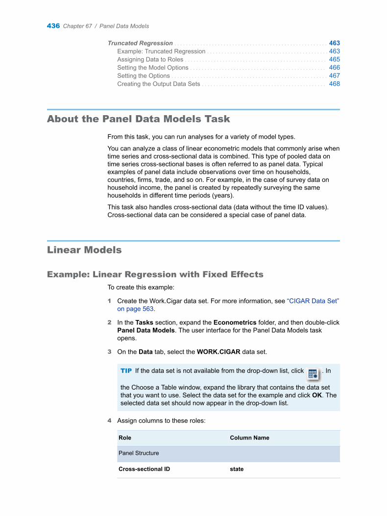
Truncated Regression . . . . . . . . . . . . . . . . . . . . . . . . . . . . . . . . . . . . . . . . . . . . . . . . . . . . . 463Example: Truncated Regression . . . . . . . . . . . . . . . . . . . . . . . . . . . . . . . . . . . . . . . . . . 463Assigning Data to Roles . . . . . . . . . . . . . . . . . . . . . . . . . . . . . . . . . . . . . . . . . . . . . . . . . 465Setting the Model Options . . . . . . . . . . . . . . . . . . . . . . . . . . . . . . . . . . . . . . . . . . . . . . . 466Setting the Options . . . . . . . . . . . . . . . . . . . . . . . . . . . . . . . . . . . . . . . . . . . . . . . . . . . . . . 467Creating the Output Data Sets . . . . . . . . . . . . . . . . . . . . . . . . . . . . . . . . . . . . . . . . . . . 468
About the Panel Data Models Task
From this task, you can run analyses for a variety of model types.
You can analyze a class of linear econometric models that commonly arise when time series and cross-sectional data is combined. This type of pooled data on time series cross-sectional bases is often referred to as panel data. Typical examples of panel data include observations over time on households, countries, firms, trade, and so on. For example, in the case of survey data on household income, the panel is created by repeatedly surveying the same households in different time periods (years).
This task also handles cross-sectional data (data without the time ID values). Cross-sectional data can be considered a special case of panel data.
Linear Models
Example: Linear Regression with Fixed Effects
To create this example:
1 Create the Work.Cigar data set. For more information, see “CIGAR Data Set” on page 563.
2 In the Tasks section, expand the Econometrics folder, and then double-click Panel Data Models. The user interface for the Panel Data Models task opens.
3 On the Data tab, select the WORK.CIGAR data set.
TIP If the data set is not available from the drop-down list, click . In
the Choose a Table window, expand the library that contains the data set that you want to use. Select the data set for the example and click OK. The selected data set should now appear in the drop-down list.
4 Assign columns to these roles:
Role Column Name
Panel Structure
Cross-sectional ID state
436 Chapter 67 / Panel Data Models
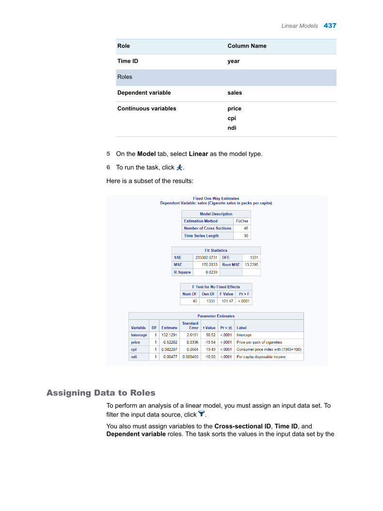
Role Column Name
Time ID year
Roles
Dependent variable sales
Continuous variables pricecpindi
5 On the Model tab, select Linear as the model type.
6 To run the task, click .
Here is a subset of the results:
Assigning Data to Roles
To perform an analysis of a linear model, you must assign an input data set. To filter the input data source, click .
You also must assign variables to the Cross-sectional ID, Time ID, and Dependent variable roles. The task sorts the values in the input data set by the
Linear Models 437
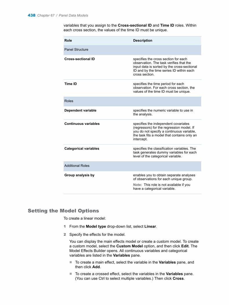
variables that you assign to the Cross-sectional ID and Time ID roles. Within each cross section, the values of the time ID must be unique.
Role Description
Panel Structure
Cross-sectional ID specifies the cross section for each observation. The task verifies that the input data is sorted by the cross-sectional ID and by the time series ID within each cross section.
Time ID specifies the time period for each observation. For each cross section, the values of the time ID must be unique.
Roles
Dependent variable specifies the numeric variable to use in the analysis.
Continuous variables specifies the independent covariates (regressors) for the regression model. If you do not specify a continuous variable, the task fits a model that contains only an intercept.
Categorical variables specifies the classification variables. The task generates dummy variables for each level of the categorical variable.
Additional Roles
Group analysis by enables you to obtain separate analyses of observations for each unique group.
Note: This role is not available if you have a categorical variable.
Setting the Model Options
To create a linear model:
1 From the Model type drop-down list, select Linear.
2 Specify the effects for the model.
You can display the main effects model or create a custom model. To create a custom model, select the Custom Model option, and then click Edit. The Model Effects Builder opens. All continuous variables and categorical variables are listed in the Variables pane.
n To create a main effect, select the variable in the Variables pane, and then click Add.
n To create a crossed effect, select the variables in the Variables pane. (You can use Ctrl to select multiple variables.) Then click Cross.
438 Chapter 67 / Panel Data Models
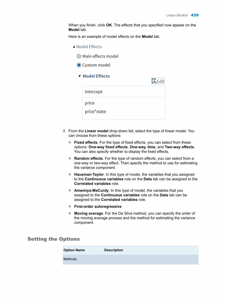
When you finish, click OK. The effects that you specified now appear on the Model tab.
Here is an example of model effects on the Model tab.
3 From the Linear model drop-down list, select the type of linear model. You can choose from these options:
n Fixed effects. For the type of fixed effects, you can select from these options: One-way fixed effects, One-way, time, and Two-way effects. You can also specify whether to display the fixed effects.
n Random effects. For the type of random effects, you can select from a one-way or two-way effect. Then specify the method to use for estimating the variance component.
n Hausman-Taylor. In this type of model, the variables that you assigned to the Continuous variables role on the Data tab can be assigned to the Correlated variables role.
n Amemiya-MaCurdy. In this type of model, the variables that you assigned to the Continuous variables role on the Data tab can be assigned to the Correlated variables role.
n First-order autoregressive
n Moving average. For the Da Silva method, you can specify the order of the moving average process and the method for estimating the variance component.
Setting the Options
Option Name Description
Methods
Linear Models 439

Option Name Description
Covariance matrix estimator
specifies the method to calculate the covariance matrix of parameter estimates.
You can use the default value, or you can choose from these methods:
n Newey and Westn OLS estimator specifies that the variance-covariance
matrix is not corrected. n HCCMEn specifies a heteroscedasticity-corrected
covariance matrix. n is a value from 0–4.
If you select one of the HCCME0-3 options for the covariance matrix estimator, you can also specify whether to include the cluster correction for the variance-covariance matrix.
Statistics
Select the statistics to display in the results.
Here are the additional statistics that you can include in the results:
n correlations of the parameter estimatesn covariances of the parameter estimatesn iteration history of the objective function and parameter estimatesn tests for random effects: one-way Breusch-Pagan test and two-way Breusch-Pagan
test
These tests are also available for first-order autoregressive linear models:n estimated covariances of the observationsn estimated autocorrelation coefficients
Plots
Select the plots to include in the results. By default, a histogram of residuals is included in the results. You can include these plots:n diagnostic plots: predicted and actual values by observation, QQ plot of residuals,
residuals by observation, and a histogram of residualsn cross-section plots: actual values by time series, predicted values by time series,
stacked residuals by time series, and residuals by time series
You can display these as a panel of plots or as individual plots. If you select Individual plots from the Display as drop-down list, you can specify the number of cross sections in one time series plot.
Creating the Output Data Sets
You can create these output data sets:
n an output data set that contains the statistics from the analysis
n a parameter estimates data set
n a transformed series data set
Note: This option is available only if you are creating a linear model that contains one-way fixed effects and one-way random effects.
440 Chapter 67 / Panel Data Models
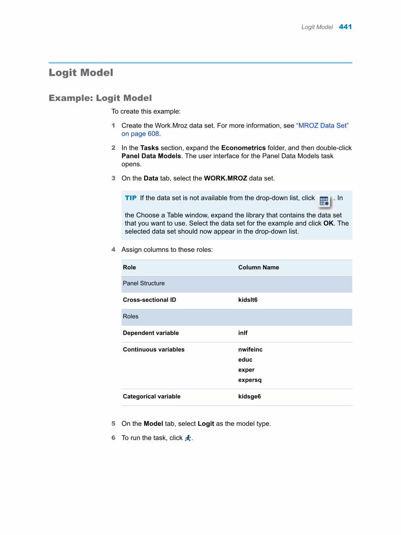
Logit Model
Example: Logit Model
To create this example:
1 Create the Work.Mroz data set. For more information, see “MROZ Data Set” on page 608.
2 In the Tasks section, expand the Econometrics folder, and then double-click Panel Data Models. The user interface for the Panel Data Models task opens.
3 On the Data tab, select the WORK.MROZ data set.
TIP If the data set is not available from the drop-down list, click . In
the Choose a Table window, expand the library that contains the data set that you want to use. Select the data set for the example and click OK. The selected data set should now appear in the drop-down list.
4 Assign columns to these roles:
Role Column Name
Panel Structure
Cross-sectional ID kidslt6
Roles
Dependent variable inlf
Continuous variables nwifeinceducexperexpersq
Categorical variable kidsge6
5 On the Model tab, select Logit as the model type.
6 To run the task, click .
Logit Model 441
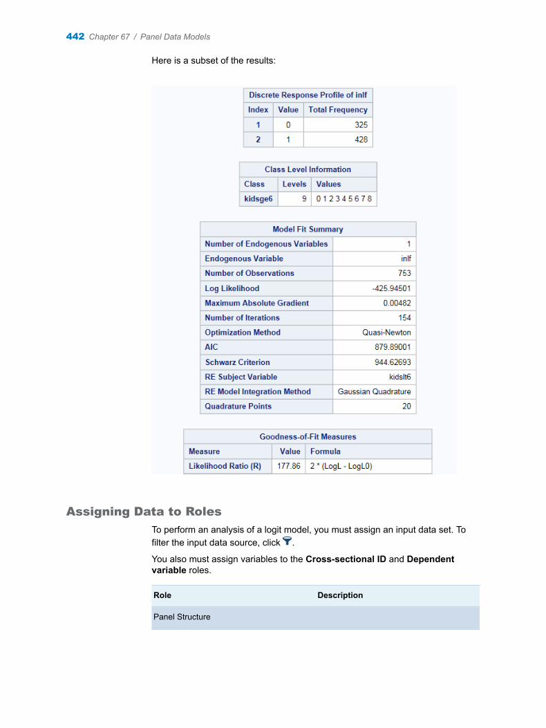
Here is a subset of the results:
Assigning Data to Roles
To perform an analysis of a logit model, you must assign an input data set. To filter the input data source, click .
You also must assign variables to the Cross-sectional ID and Dependent variable roles.
Role Description
Panel Structure
442 Chapter 67 / Panel Data Models
Role Description
Cross-sectional ID specifies the cross section for each observation. The task verifies that the input data is sorted by the cross-sectional ID.
Note: For the logit model, character variables are not supported.
Time ID specifies the time period for each observation. For each cross section, the values of the time ID must be unique.
Note: For the logit model, a time ID is not required and is ignored in the analysis.
Roles
Dependent variable specifies the numeric variable that takes discrete values.
Continuous variables specifies the classification variables. The task generates dummy variables for each level of the categorical variable.
Categorical variables specifies the independent covariates (regressors) for the regression model. If you do not specify a continuous variable, the task fits a model that contains only an intercept.
Additional Roles
Group analysis by enables you to obtain separate analyses of observations for each unique group.
Setting the Model Options
To create a logit model:
1 From the Model type drop-down list, select Logit.
2 Specify the effects for the model.
You can display the main effects model or create a custom model. To create a custom model, select the Custom Model option, and then click Edit. The Model Effects Builder opens. All continuous variables and categorical variables are listed in the Variables pane.
n To create a main effect, select the variable in the Variables pane, and then click Add.
n To create a crossed effect, select the variables in the Variables pane. (You can use Ctrl to select multiple variables.) Then click Cross.
When you finish, click OK. The effects that you specified now appear on the Model tab.
Logit Model 443
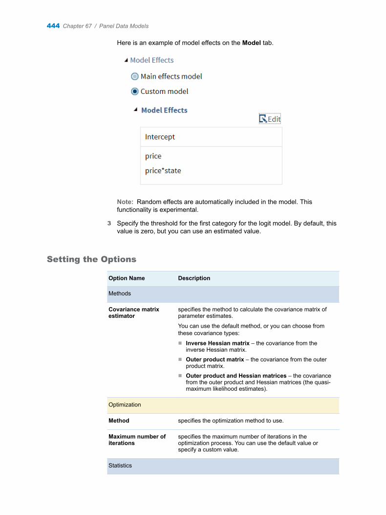
Here is an example of model effects on the Model tab.
Note: Random effects are automatically included in the model. This functionality is experimental.
3 Specify the threshold for the first category for the logit model. By default, this value is zero, but you can use an estimated value.
Setting the Options
Option Name Description
Methods
Covariance matrix estimator
specifies the method to calculate the covariance matrix of parameter estimates.
You can use the default method, or you can choose from these covariance types:
n Inverse Hessian matrix – the covariance from the inverse Hessian matrix.
n Outer product matrix – the covariance from the outer product matrix.
n Outer product and Hessian matrices – the covariance from the outer product and Hessian matrices (the quasi-maximum likelihood estimates).
Optimization
Method specifies the optimization method to use.
Maximum number of iterations
specifies the maximum number of iterations in the optimization process. You can use the default value or specify a custom value.
Statistics
444 Chapter 67 / Panel Data Models
Option Name Description
Select the statistics to display in the results.
Here are the additional statistics that you can include in the results:
n correlations of the parameter estimatesn covariances of the parameter estimatesn iteration history of the objective function and parameter estimates
Plots
You can choose to display only the default plots, the selected plots, or no plots in the results.
You can choose from these types of plots:
n diagnostic plots, such as error standard deviations by observed regressor and profiled log likelihood
n output plots, such as predicted values by regressor, marginal effects by regressor, Inverse Mills ratio by regressor, predicted response probability by regressor, predicted probabilities for each level of the response by regressor, and linear predictor values by regressor
Creating the Output Data Sets
You can create these output data sets:
n an output data set that contains the default statistics from the analysis and additional statistics, such as predicted values, the probability of the dependent variable taking the current value, the probability of the dependent variable for all possible responses, and the error standard deviation
n a parameter estimates data set
Probit Model
Example: Probit Model
To create this example:
1 Create the Work.Moz data set. For more information, see “MROZ Data Set” on page 608.
2 In the Tasks section, expand the Econometrics folder, and then double-click Panel Data Models. The user interface for the Panel Data Models task opens.
3 On the Data tab, select the WORK.MROZ data set.
TIP If the data set is not available from the drop-down list, click . In
the Choose a Table window, expand the library that contains the data set
Probit Model 445
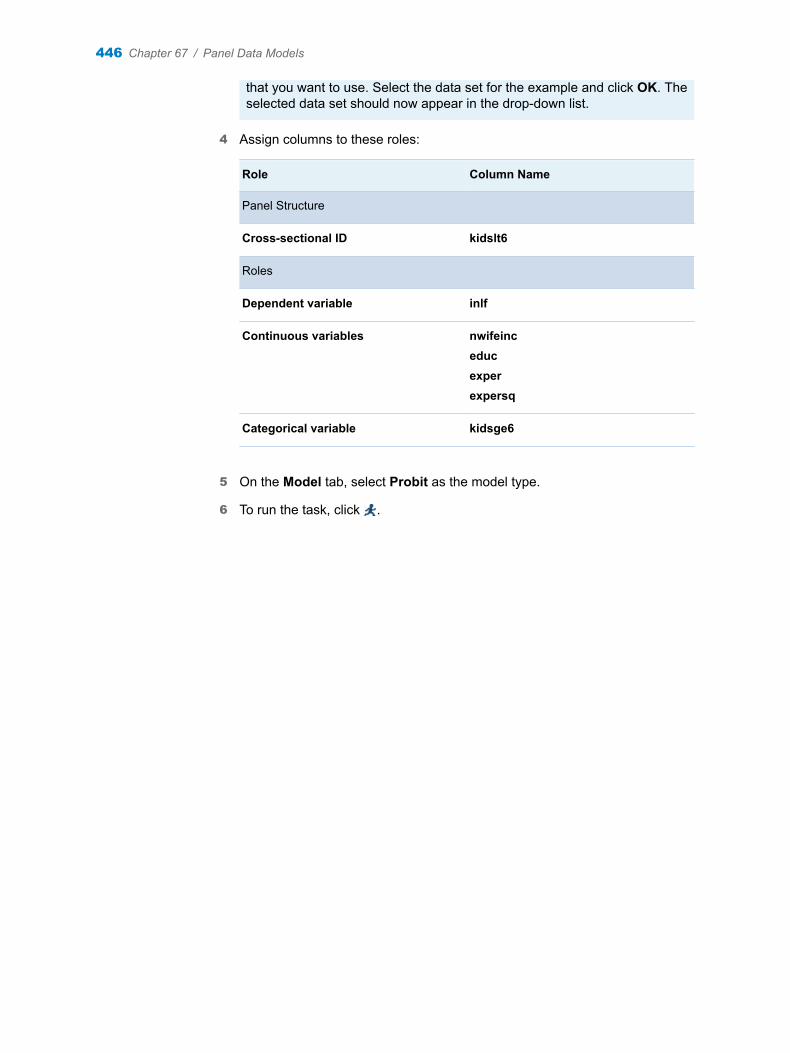
that you want to use. Select the data set for the example and click OK. The selected data set should now appear in the drop-down list.
4 Assign columns to these roles:
Role Column Name
Panel Structure
Cross-sectional ID kidslt6
Roles
Dependent variable inlf
Continuous variables nwifeinceducexperexpersq
Categorical variable kidsge6
5 On the Model tab, select Probit as the model type.
6 To run the task, click .
446 Chapter 67 / Panel Data Models
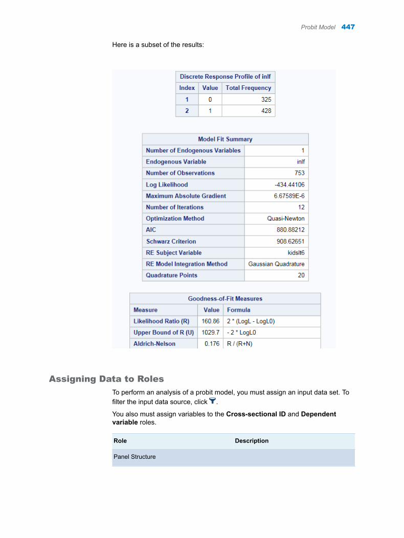
Here is a subset of the results:
Assigning Data to Roles
To perform an analysis of a probit model, you must assign an input data set. To filter the input data source, click .
You also must assign variables to the Cross-sectional ID and Dependent variable roles.
Role Description
Panel Structure
Probit Model 447
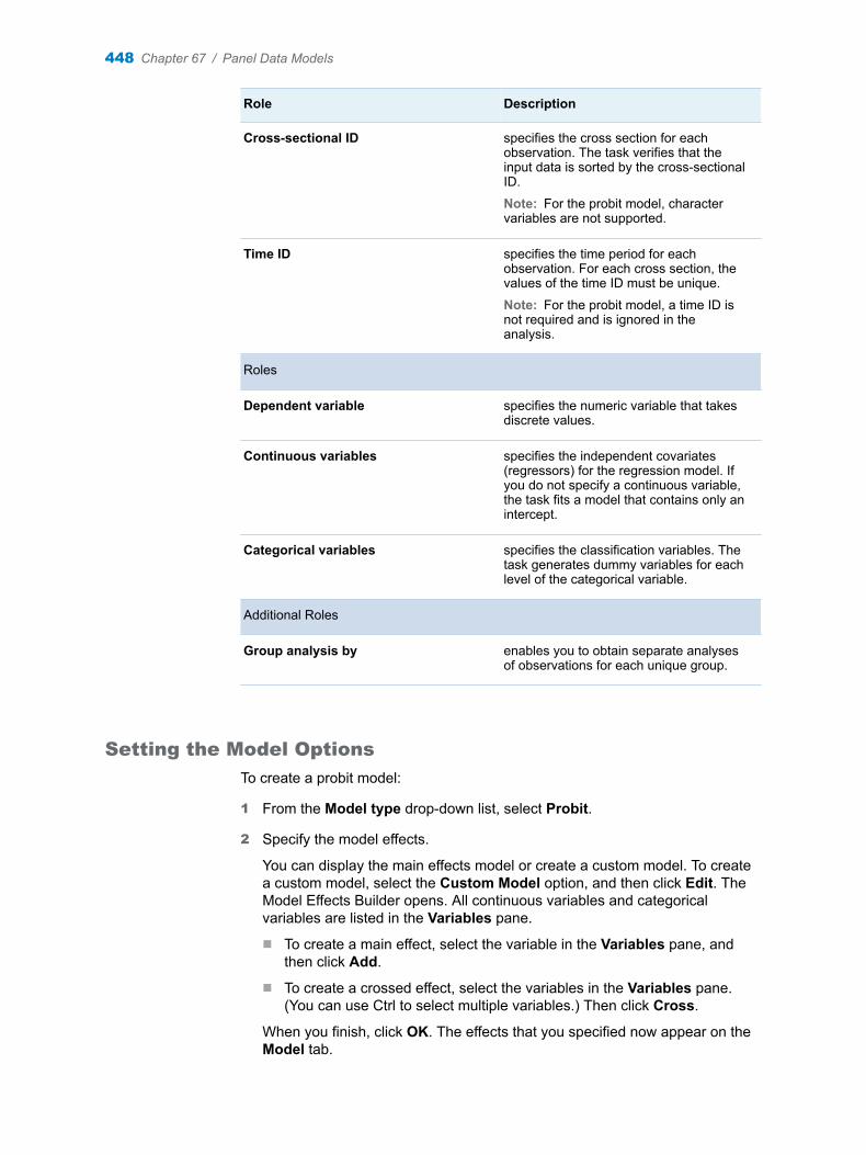
Role Description
Cross-sectional ID specifies the cross section for each observation. The task verifies that the input data is sorted by the cross-sectional ID.
Note: For the probit model, character variables are not supported.
Time ID specifies the time period for each observation. For each cross section, the values of the time ID must be unique.
Note: For the probit model, a time ID is not required and is ignored in the analysis.
Roles
Dependent variable specifies the numeric variable that takes discrete values.
Continuous variables specifies the independent covariates (regressors) for the regression model. If you do not specify a continuous variable, the task fits a model that contains only an intercept.
Categorical variables specifies the classification variables. The task generates dummy variables for each level of the categorical variable.
Additional Roles
Group analysis by enables you to obtain separate analyses of observations for each unique group.
Setting the Model Options
To create a probit model:
1 From the Model type drop-down list, select Probit.
2 Specify the model effects.
You can display the main effects model or create a custom model. To create a custom model, select the Custom Model option, and then click Edit. The Model Effects Builder opens. All continuous variables and categorical variables are listed in the Variables pane.
n To create a main effect, select the variable in the Variables pane, and then click Add.
n To create a crossed effect, select the variables in the Variables pane. (You can use Ctrl to select multiple variables.) Then click Cross.
When you finish, click OK. The effects that you specified now appear on the Model tab.
448 Chapter 67 / Panel Data Models
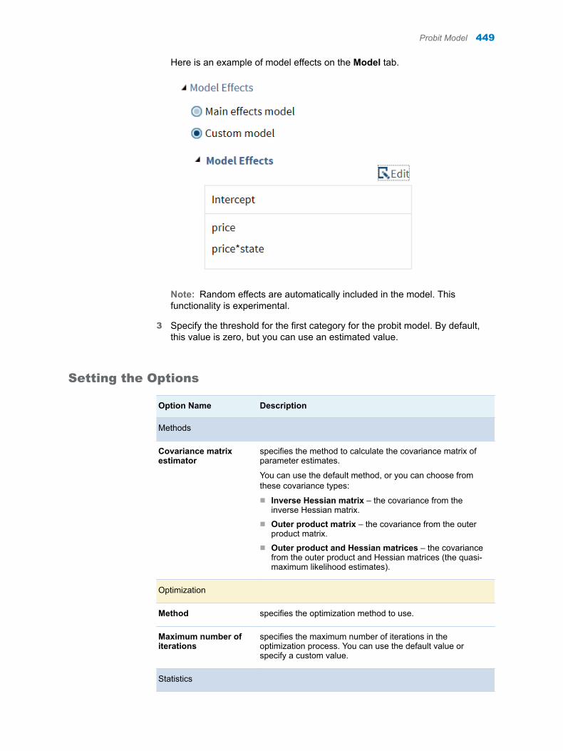
Here is an example of model effects on the Model tab.
Note: Random effects are automatically included in the model. This functionality is experimental.
3 Specify the threshold for the first category for the probit model. By default, this value is zero, but you can use an estimated value.
Setting the Options
Option Name Description
Methods
Covariance matrix estimator
specifies the method to calculate the covariance matrix of parameter estimates.
You can use the default method, or you can choose from these covariance types:
n Inverse Hessian matrix – the covariance from the inverse Hessian matrix.
n Outer product matrix – the covariance from the outer product matrix.
n Outer product and Hessian matrices – the covariance from the outer product and Hessian matrices (the quasi-maximum likelihood estimates).
Optimization
Method specifies the optimization method to use.
Maximum number of iterations
specifies the maximum number of iterations in the optimization process. You can use the default value or specify a custom value.
Statistics
Probit Model 449
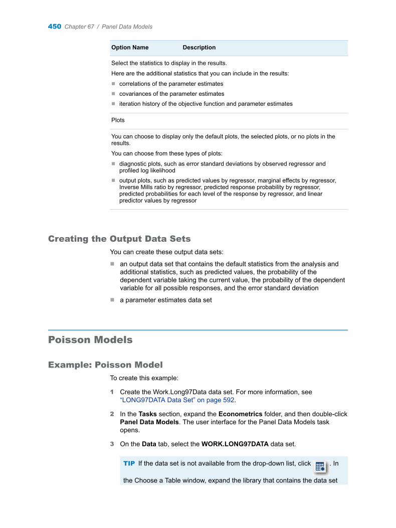
Option Name Description
Select the statistics to display in the results.
Here are the additional statistics that you can include in the results:
n correlations of the parameter estimatesn covariances of the parameter estimatesn iteration history of the objective function and parameter estimates
Plots
You can choose to display only the default plots, the selected plots, or no plots in the results.
You can choose from these types of plots:
n diagnostic plots, such as error standard deviations by observed regressor and profiled log likelihood
n output plots, such as predicted values by regressor, marginal effects by regressor, Inverse Mills ratio by regressor, predicted response probability by regressor, predicted probabilities for each level of the response by regressor, and linear predictor values by regressor
Creating the Output Data Sets
You can create these output data sets:
n an output data set that contains the default statistics from the analysis and additional statistics, such as predicted values, the probability of the dependent variable taking the current value, the probability of the dependent variable for all possible responses, and the error standard deviation
n a parameter estimates data set
Poisson Models
Example: Poisson Model
To create this example:
1 Create the Work.Long97Data data set. For more information, see “LONG97DATA Data Set” on page 592.
2 In the Tasks section, expand the Econometrics folder, and then double-click Panel Data Models. The user interface for the Panel Data Models task opens.
3 On the Data tab, select the WORK.LONG97DATA data set.
TIP If the data set is not available from the drop-down list, click . In
the Choose a Table window, expand the library that contains the data set
450 Chapter 67 / Panel Data Models
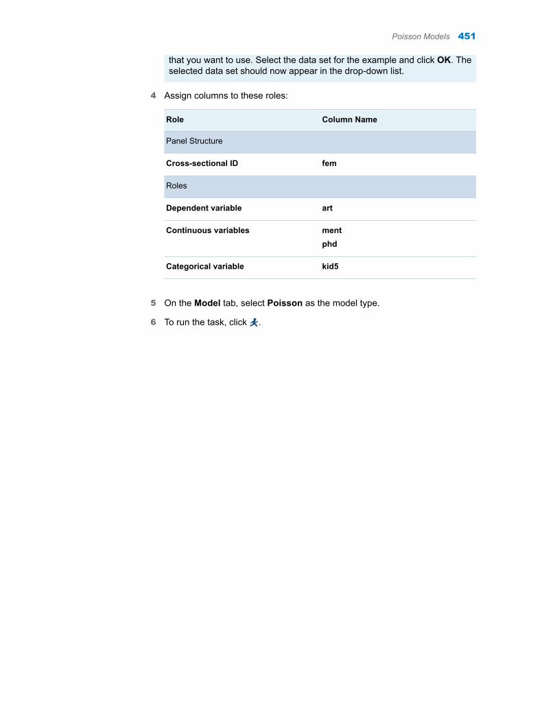
that you want to use. Select the data set for the example and click OK. The selected data set should now appear in the drop-down list.
4 Assign columns to these roles:
Role Column Name
Panel Structure
Cross-sectional ID fem
Roles
Dependent variable art
Continuous variables mentphd
Categorical variable kid5
5 On the Model tab, select Poisson as the model type.
6 To run the task, click .
Poisson Models 451
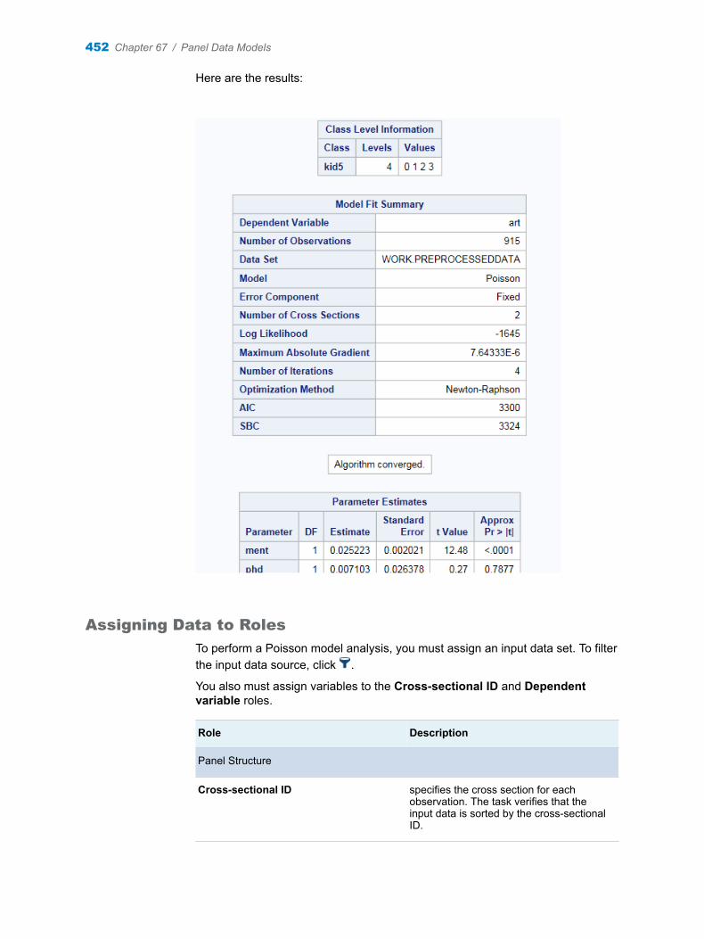
Here are the results:
Assigning Data to Roles
To perform a Poisson model analysis, you must assign an input data set. To filter the input data source, click .
You also must assign variables to the Cross-sectional ID and Dependent variable roles.
Role Description
Panel Structure
Cross-sectional ID specifies the cross section for each observation. The task verifies that the input data is sorted by the cross-sectional ID.
452 Chapter 67 / Panel Data Models
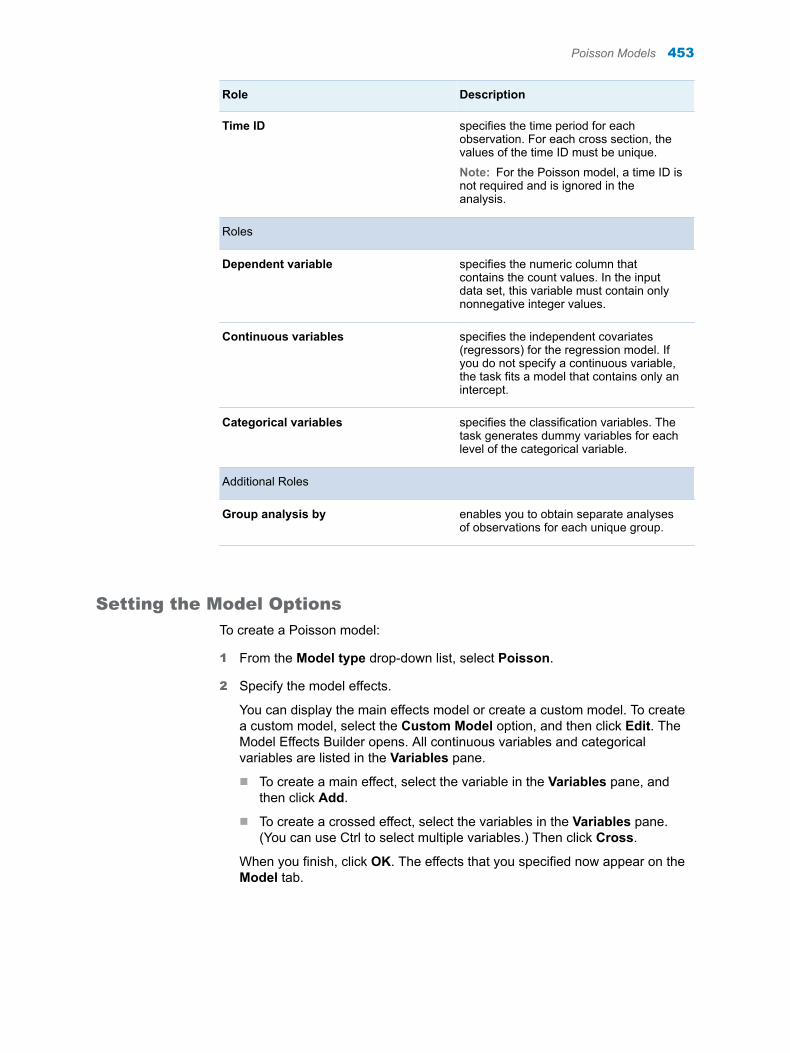
Role Description
Time ID specifies the time period for each observation. For each cross section, the values of the time ID must be unique.
Note: For the Poisson model, a time ID is not required and is ignored in the analysis.
Roles
Dependent variable specifies the numeric column that contains the count values. In the input data set, this variable must contain only nonnegative integer values.
Continuous variables specifies the independent covariates (regressors) for the regression model. If you do not specify a continuous variable, the task fits a model that contains only an intercept.
Categorical variables specifies the classification variables. The task generates dummy variables for each level of the categorical variable.
Additional Roles
Group analysis by enables you to obtain separate analyses of observations for each unique group.
Setting the Model Options
To create a Poisson model:
1 From the Model type drop-down list, select Poisson.
2 Specify the model effects.
You can display the main effects model or create a custom model. To create a custom model, select the Custom Model option, and then click Edit. The Model Effects Builder opens. All continuous variables and categorical variables are listed in the Variables pane.
n To create a main effect, select the variable in the Variables pane, and then click Add.
n To create a crossed effect, select the variables in the Variables pane. (You can use Ctrl to select multiple variables.) Then click Cross.
When you finish, click OK. The effects that you specified now appear on the Model tab.
Poisson Models 453
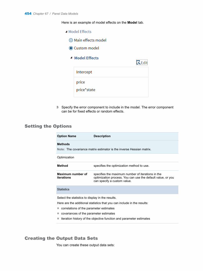
Here is an example of model effects on the Model tab.
3 Specify the error component to include in the model. The error component can be for fixed effects or random effects.
Setting the Options
Option Name Description
MethodsNote: The covariance matrix estimator is the inverse Hessian matrix.
Optimization
Method specifies the optimization method to use.
Maximum number of iterations
specifies the maximum number of iterations in the optimization process. You can use the default value, or you can specify a custom value.
Statistics
Select the statistics to display in the results.
Here are the additional statistics that you can include in the results:
n correlations of the parameter estimatesn covariances of the parameter estimatesn iteration history of the objective function and parameter estimates
Creating the Output Data Sets
You can create these output data sets:
454 Chapter 67 / Panel Data Models
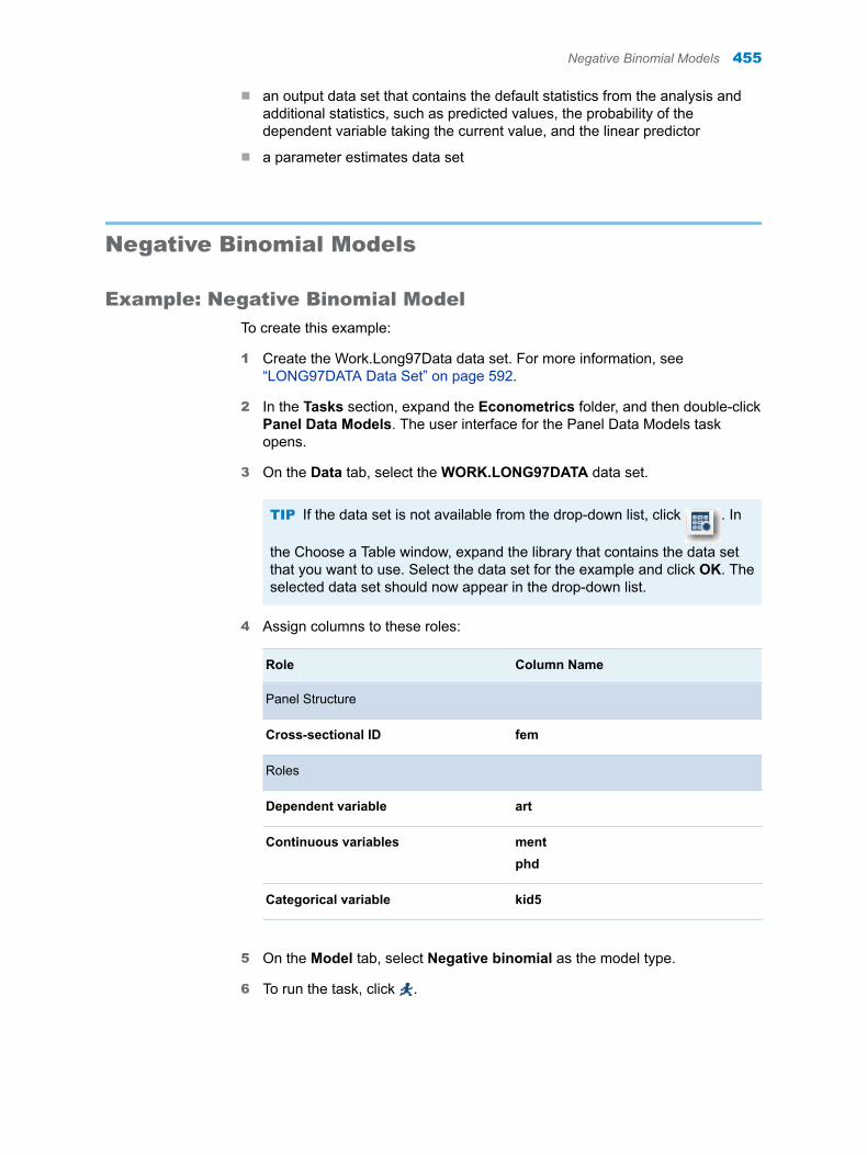
n an output data set that contains the default statistics from the analysis and additional statistics, such as predicted values, the probability of the dependent variable taking the current value, and the linear predictor
n a parameter estimates data set
Negative Binomial Models
Example: Negative Binomial Model
To create this example:
1 Create the Work.Long97Data data set. For more information, see “LONG97DATA Data Set” on page 592.
2 In the Tasks section, expand the Econometrics folder, and then double-click Panel Data Models. The user interface for the Panel Data Models task opens.
3 On the Data tab, select the WORK.LONG97DATA data set.
TIP If the data set is not available from the drop-down list, click . In
the Choose a Table window, expand the library that contains the data set that you want to use. Select the data set for the example and click OK. The selected data set should now appear in the drop-down list.
4 Assign columns to these roles:
Role Column Name
Panel Structure
Cross-sectional ID fem
Roles
Dependent variable art
Continuous variables mentphd
Categorical variable kid5
5 On the Model tab, select Negative binomial as the model type.
6 To run the task, click .
Negative Binomial Models 455
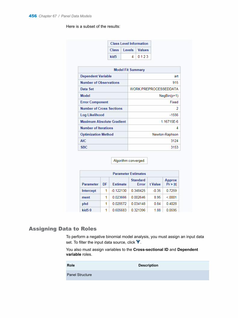
Here is a subset of the results:
Assigning Data to Roles
To perform a negative binomial model analysis, you must assign an input data set. To filter the input data source, click .
You also must assign variables to the Cross-sectional ID and Dependent variable roles.
Role Description
Panel Structure
456 Chapter 67 / Panel Data Models
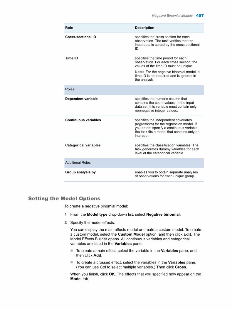
Role Description
Cross-sectional ID specifies the cross section for each observation. The task verifies that the input data is sorted by the cross-sectional ID.
Time ID specifies the time period for each observation. For each cross section, the values of the time ID must be unique.
Note: For the negative binomial model, a time ID is not required and is ignored in the analysis.
Roles
Dependent variable specifies the numeric column that contains the count values. In the input data set, this variable must contain only nonnegative integer values.
Continuous variables specifies the independent covariates (regressors) for the regression model. If you do not specify a continuous variable, the task fits a model that contains only an intercept.
Categorical variables specifies the classification variables. The task generates dummy variables for each level of the categorical variable.
Additional Roles
Group analysis by enables you to obtain separate analyses of observations for each unique group.
Setting the Model Options
To create a negative binomial model:
1 From the Model type drop-down list, select Negative binomial.
2 Specify the model effects.
You can display the main effects model or create a custom model. To create a custom model, select the Custom Model option, and then click Edit. The Model Effects Builder opens. All continuous variables and categorical variables are listed in the Variables pane.
n To create a main effect, select the variable in the Variables pane, and then click Add.
n To create a crossed effect, select the variables in the Variables pane. (You can use Ctrl to select multiple variables.) Then click Cross.
When you finish, click OK. The effects that you specified now appear on the Model tab.
Negative Binomial Models 457
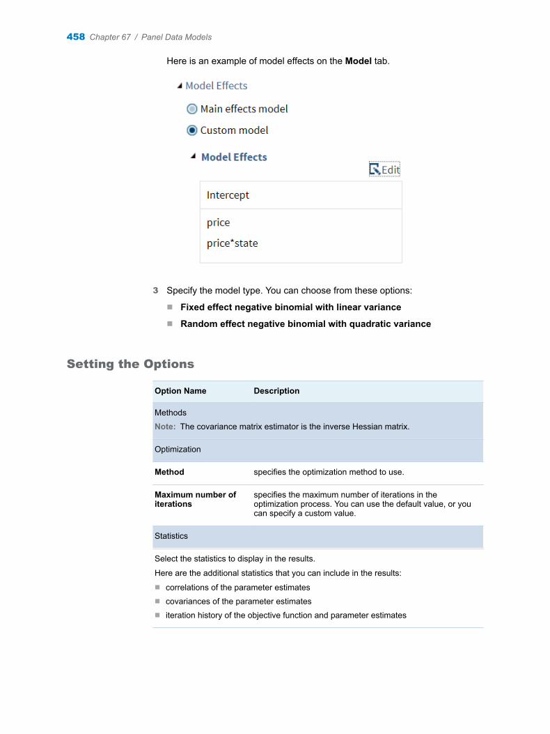
Here is an example of model effects on the Model tab.
3 Specify the model type. You can choose from these options:
n Fixed effect negative binomial with linear variance
n Random effect negative binomial with quadratic variance
Setting the Options
Option Name Description
Methods
Note: The covariance matrix estimator is the inverse Hessian matrix.
Optimization
Method specifies the optimization method to use.
Maximum number of iterations
specifies the maximum number of iterations in the optimization process. You can use the default value, or you can specify a custom value.
Statistics
Select the statistics to display in the results.
Here are the additional statistics that you can include in the results:
n correlations of the parameter estimatesn covariances of the parameter estimatesn iteration history of the objective function and parameter estimates
458 Chapter 67 / Panel Data Models
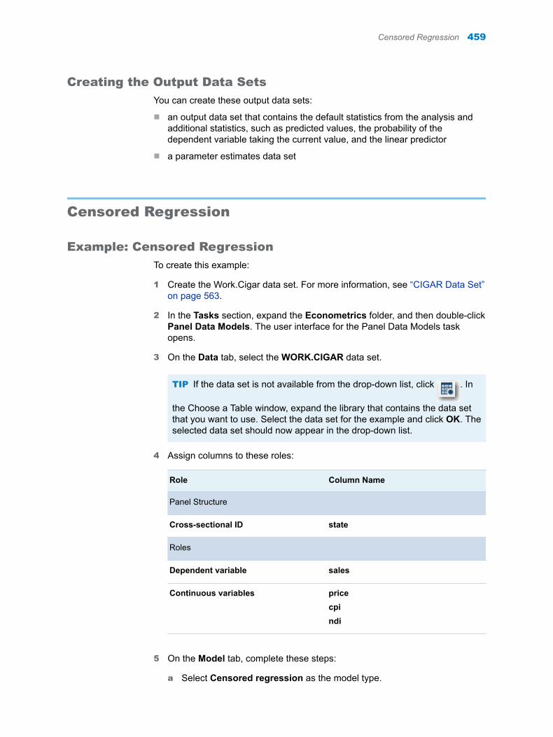
Creating the Output Data Sets
You can create these output data sets:
n an output data set that contains the default statistics from the analysis and additional statistics, such as predicted values, the probability of the dependent variable taking the current value, and the linear predictor
n a parameter estimates data set
Censored Regression
Example: Censored Regression
To create this example:
1 Create the Work.Cigar data set. For more information, see “CIGAR Data Set” on page 563.
2 In the Tasks section, expand the Econometrics folder, and then double-click Panel Data Models. The user interface for the Panel Data Models task opens.
3 On the Data tab, select the WORK.CIGAR data set.
TIP If the data set is not available from the drop-down list, click . In
the Choose a Table window, expand the library that contains the data set that you want to use. Select the data set for the example and click OK. The selected data set should now appear in the drop-down list.
4 Assign columns to these roles:
Role Column Name
Panel Structure
Cross-sectional ID state
Roles
Dependent variable sales
Continuous variables pricecpindi
5 On the Model tab, complete these steps:
a Select Censored regression as the model type.
Censored Regression 459
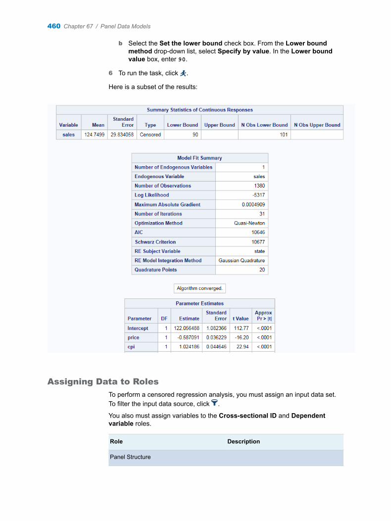
b Select the Set the lower bound check box. From the Lower bound method drop-down list, select Specify by value. In the Lower bound value box, enter 90.
6 To run the task, click .
Here is a subset of the results:
Assigning Data to Roles
To perform a censored regression analysis, you must assign an input data set. To filter the input data source, click .
You also must assign variables to the Cross-sectional ID and Dependent variable roles.
Role Description
Panel Structure
460 Chapter 67 / Panel Data Models

Role Description
Cross-sectional ID specifies the cross section for each observation. The task verifies that the input data is sorted by the cross-sectional ID.
Note: For the censored regression model, character variables are not supported.
Time ID specifies the time period for each observation. For each cross section, the values of the time ID must be unique.
Note: For the censored regression model, a time ID is not required and is ignored in the analysis.
Roles
Dependent variable specifies the numeric variable for the analysis.
Continuous variables specifies the independent covariates (regressors) for the regression model. If you do not specify a continuous variable, the task fits a model that contains only an intercept.
Categorical variables specifies the classification variables. The task generates dummy variables for each level of the categorical variable.
Additional Roles
Group analysis by enables you to obtain separate analyses of observations for each unique group.
Setting the Model Options
To create a censored regression model:
1 From the Model type drop-down list, select Censored regression.
2 Specify the model effects.
You can display the main effects model or create a custom model. To create a custom model, select the Custom Model option, and then click Edit. The Model Effects Builder opens. All continuous variables and categorical variables are listed in the Variables pane.
n To create a main effect, select the variable in the Variables pane, and then click Add.
n To create a crossed effect, select the variables in the Variables pane. (You can use Ctrl to select multiple variables.) Then click Cross.
When you finish, click OK. The effects that you specified now appear on the Model tab.
Censored Regression 461
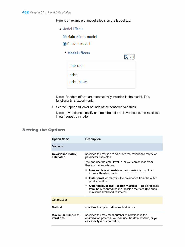
Here is an example of model effects on the Model tab.
Note: Random effects are automatically included in the model. This functionality is experimental.
3 Set the upper and lower bounds of the censored variables.
Note: If you do not specify an upper bound or a lower bound, the result is a linear regression model.
Setting the Options
Option Name Description
Methods
Covariance matrix estimator
specifies the method to calculate the covariance matrix of parameter estimates.
You can use the default value, or you can choose from these covariance types:
n Inverse Hessian matrix – the covariance from the inverse Hessian matrix.
n Outer product matrix – the covariance from the outer product matrix.
n Outer product and Hessian matrices – the covariance from the outer product and Hessian matrices (the quasi-maximum likelihood estimates).
Optimization
Method specifies the optimization method to use.
Maximum number of iterations
specifies the maximum number of iterations in the optimization process. You can use the default value, or you can specify a custom value.
462 Chapter 67 / Panel Data Models

Option Name Description
Statistics
Select the statistics to display in the results.
Here are the additional statistics that you can include in the results:
n correlations of the parameter estimatesn covariances of the parameter estimatesn iteration history of the objective function and parameter estimates
Creating the Output Data Sets
You can create these output data sets:
n an output data set that contains the default statistics from the analysis and additional statistics, such as predicted values, residuals, the error standard deviation, and the linear predictor
n a parameter estimates data set
Truncated Regression
Example: Truncated Regression
To create this example:
1 Create the Work.Cigar data set. For more information, see “CIGAR Data Set” on page 563.
2 In the Tasks section, expand the Econometrics folder, and then double-click Panel Data Models. The user interface for the Panel Data Models task opens.
3 On the Data tab, select the WORK.CIGAR data set.
TIP If the data set is not available from the drop-down list, click . In
the Choose a Table window, expand the library that contains the data set that you want to use. Select the data set for the example and click OK. The selected data set should now appear in the drop-down list.
4 Assign columns to these roles:
Role Column Name
Panel Structure
Cross-sectional ID state
Truncated Regression 463

Role Column Name
Roles
Dependent variable sales
Continuous variables pricecpindi
5 On the Model tab, complete these steps:
a Select Truncated regression as the model type.
b Select the Set the lower bound check box. From the Lower bound method drop-down list, select Specify by value. In the Lower bound value box, enter 90.
6 To run the task, click .
464 Chapter 67 / Panel Data Models
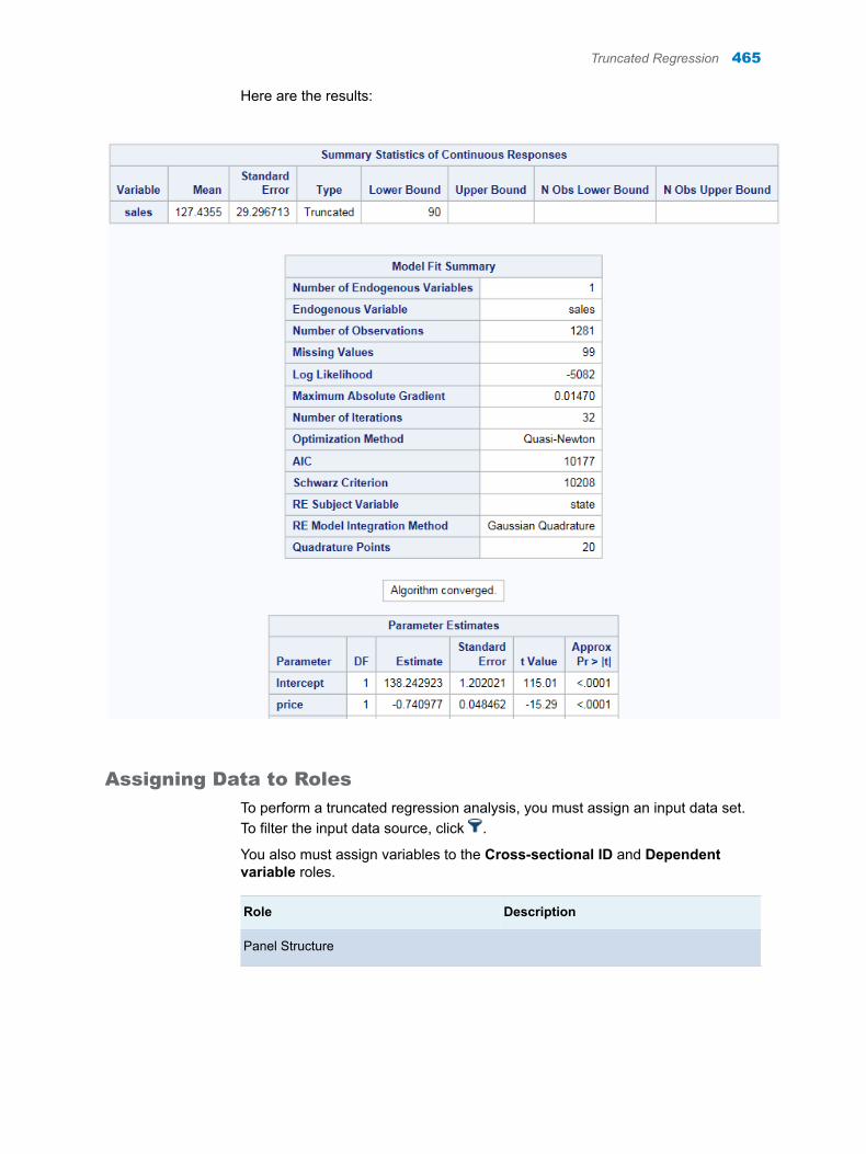
Here are the results:
Assigning Data to Roles
To perform a truncated regression analysis, you must assign an input data set. To filter the input data source, click .
You also must assign variables to the Cross-sectional ID and Dependent variable roles.
Role Description
Panel Structure
Truncated Regression 465
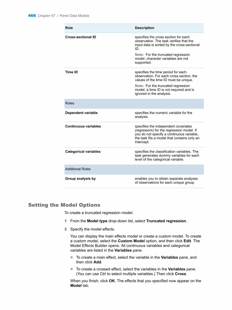
Role Description
Cross-sectional ID specifies the cross section for each observation. The task verifies that the input data is sorted by the cross-sectional ID.
Note: For the truncated regression model, character variables are not supported.
Time ID specifies the time period for each observation. For each cross section, the values of the time ID must be unique.
Note: For the truncated regression model, a time ID is not required and is ignored in the analysis.
Roles
Dependent variable specifies the numeric variable for the analysis.
Continuous variables specifies the independent covariates (regressors) for the regression model. If you do not specify a continuous variable, the task fits a model that contains only an intercept.
Categorical variables specifies the classification variables. The task generates dummy variables for each level of the categorical variable.
Additional Roles
Group analysis by enables you to obtain separate analyses of observations for each unique group.
Setting the Model Options
To create a truncated regression model:
1 From the Model type drop-down list, select Truncated regression.
2 Specify the model effects.
You can display the main effects model or create a custom model. To create a custom model, select the Custom Model option, and then click Edit. The Model Effects Builder opens. All continuous variables and categorical variables are listed in the Variables pane.
n To create a main effect, select the variable in the Variables pane, and then click Add.
n To create a crossed effect, select the variables in the Variables pane. (You can use Ctrl to select multiple variables.) Then click Cross.
When you finish, click OK. The effects that you specified now appear on the Model tab.
466 Chapter 67 / Panel Data Models

Here is an example of model effects on the Model tab.
Note: Random effects are automatically included in the model. This functionality is experimental.
3 Set the upper and lower bounds of the censored variables.
Note: If you do not specify an upper bound or a lower bound, the result is a linear regression model.
Setting the Options
Option Name Description
Methods
Covariance matrix estimator
specifies the method to calculate the covariance matrix of parameter estimates.
You can use the default value, or you can choose from these covariance types:
n Inverse Hessian matrix – the covariance from the inverse Hessian matrix.
n Outer product matrix – the covariance from the outer product matrix.
n Outer product and Hessian matrices – the covariance from the outer product and Hessian matrices (the quasi-maximum likelihood estimates).
Optimization
Method specifies the optimization method to use.
Maximum number of iterations
specifies the maximum number of iterations in the optimization process. You can use the default value, or you can specify a custom value.
Truncated Regression 467
Option Name Description
Statistics
Select the statistics to display in the results.
Here are the additional statistics that you can include in the results:
n correlations of the parameter estimatesn covariances of the parameter estimatesn iteration history of the objective function and parameter estimates
Creating the Output Data Sets
You can create these output data sets:
n an output data set that contains the default statistics from the analysis and additional statistics, such as predicted values, residuals, the error standard deviation, and the linear predictor
n a parameter estimates data set
468 Chapter 67 / Panel Data Models
68Time Series Analysis
About the Time Series Analysis Task . . . . . . . . . . . . . . . . . . . . . . . . . . . . . . . . . . . . . . 469
Time Series Analysis for One Dependent Variable . . . . . . . . . . . . . . . . . . . . . . . . . 469Example: Analyzing Sales Data . . . . . . . . . . . . . . . . . . . . . . . . . . . . . . . . . . . . . . . . . . 469Assigning Data to Roles . . . . . . . . . . . . . . . . . . . . . . . . . . . . . . . . . . . . . . . . . . . . . . . . . 471Setting the Model Options . . . . . . . . . . . . . . . . . . . . . . . . . . . . . . . . . . . . . . . . . . . . . . . 472Setting the Options . . . . . . . . . . . . . . . . . . . . . . . . . . . . . . . . . . . . . . . . . . . . . . . . . . . . . . 474Creating an Output Data Set . . . . . . . . . . . . . . . . . . . . . . . . . . . . . . . . . . . . . . . . . . . . . 475
Time Series Analysis for Multiple Dependent Variables . . . . . . . . . . . . . . . . . . . . 475Example: Analyzing Sales and Cost Data . . . . . . . . . . . . . . . . . . . . . . . . . . . . . . . . . 475Assigning Data to Roles . . . . . . . . . . . . . . . . . . . . . . . . . . . . . . . . . . . . . . . . . . . . . . . . . 476Setting the Model Options . . . . . . . . . . . . . . . . . . . . . . . . . . . . . . . . . . . . . . . . . . . . . . . 477Setting the Options . . . . . . . . . . . . . . . . . . . . . . . . . . . . . . . . . . . . . . . . . . . . . . . . . . . . . . 479Creating an Output Data Set . . . . . . . . . . . . . . . . . . . . . . . . . . . . . . . . . . . . . . . . . . . . . 480
About the Time Series Analysis Task
The Time Series Analysis task fits models to equally spaced time series data of any frequency, such as monthly, quarterly, or weekly data. You can have a single dependent variable or multiple dependent variables. You can also include one or more explanatory variables in the model. The time series could be correlated over time with either constant variance or non-constant variance. The family of GARCH models are used to model series with non-constant (heteroscedastic) variance.
Time Series Analysis for One Dependent Variable
Example: Analyzing Sales Data
To create this example:
1 In the Tasks section, expand the Econometrics folder, and then double-click Time Series Analysis. The user interface for the Time Series Analysis task opens.
469
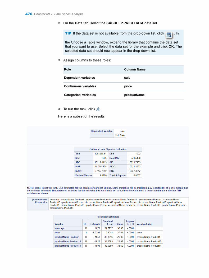
2 On the Data tab, select the SASHELP.PRICEDATA data set.
TIP If the data set is not available from the drop-down list, click . In
the Choose a Table window, expand the library that contains the data set that you want to use. Select the data set for the example and click OK. The selected data set should now appear in the drop-down list.
3 Assign columns to these roles:
Role Column Name
Dependent variables sale
Continuous variables price
Categorical variables productName
4 To run the task, click .
Here is a subset of the results:
470 Chapter 68 / Time Series Analysis
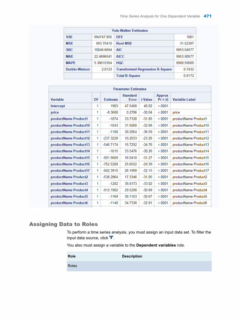
Assigning Data to Roles
To perform a time series analysis, you must assign an input data set. To filter the input data source, click .
You also must assign a variable to the Dependent variables role.
Role Description
Roles
Time Series Analysis for One Dependent Variable 471
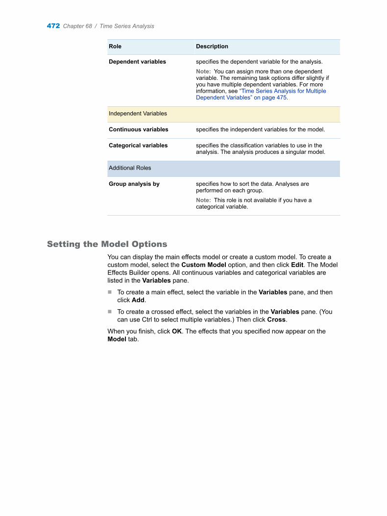
Role Description
Dependent variables specifies the dependent variable for the analysis.
Note: You can assign more than one dependent variable. The remaining task options differ slightly if you have multiple dependent variables. For more information, see “Time Series Analysis for Multiple Dependent Variables” on page 475.
Independent Variables
Continuous variables specifies the independent variables for the model.
Categorical variables specifies the classification variables to use in the analysis. The analysis produces a singular model.
Additional Roles
Group analysis by specifies how to sort the data. Analyses are performed on each group.
Note: This role is not available if you have a categorical variable.
Setting the Model Options
You can display the main effects model or create a custom model. To create a custom model, select the Custom Model option, and then click Edit. The Model Effects Builder opens. All continuous variables and categorical variables are listed in the Variables pane.
n To create a main effect, select the variable in the Variables pane, and then click Add.
n To create a crossed effect, select the variables in the Variables pane. (You can use Ctrl to select multiple variables.) Then click Cross.
When you finish, click OK. The effects that you specified now appear on the Model tab.
472 Chapter 68 / Time Series Analysis
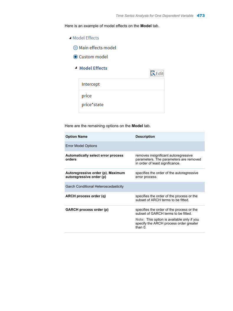
Here is an example of model effects on the Model tab.
Here are the remaining options on the Model tab.
Option Name Description
Error Model Options
Automatically select error process orders
removes insignificant autoregressive parameters. The parameters are removed in order of least significance.
Autoregressive order (p), Maximum autoregressive order (p)
specifies the order of the autoregressive error process.
Garch Conditional Heteroscedasticity
ARCH process order (q) specifies the order of the process or the subset of ARCH terms to be fitted.
GARCH process order (p) specifies the order of the process or the subset of GARCH terms to be fitted.
Note: This option is available only if you specify the ARCH process order greater than 0.
Time Series Analysis for One Dependent Variable 473
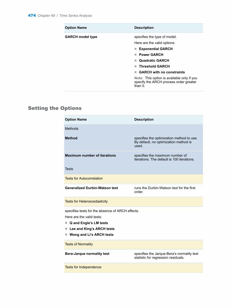
Option Name Description
GARCH model type specifies the type of model.
Here are the valid options:
n Exponential GARCHn Power GARCHn Quadratic GARCHn Threshold GARCHn GARCH with no constraintsNote: This option is available only if you specify the ARCH process order greater than 0.
Setting the Options
Option Name Description
Methods
Method specifies the optimization method to use. By default, no optimization method is used.
Maximum number of iterations specifies the maximum number of iterations. The default is 100 iterations.
Tests
Tests for Autocorrelation
Generalized Durbin-Watson test runs the Durbin-Watson test for the first order.
Tests for Heteroscedasticity
specifies tests for the absence of ARCH effects.
Here are the valid tests:
n Q and Engle’s LM testsn Lee and King’s ARCH testsn Wong and Li’s ARCH tests
Tests of Normality
Bera-Jarque normality test specifies the Jarque-Bera’s normality test statistic for regression residuals.
Tests for Independence
474 Chapter 68 / Time Series Analysis
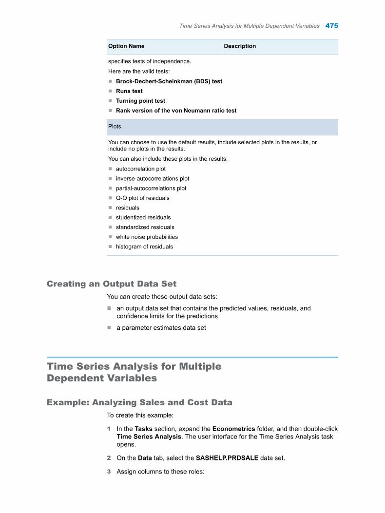
Option Name Description
specifies tests of independence.
Here are the valid tests:
n Brock-Dechert-Scheinkman (BDS) testn Runs testn Turning point testn Rank version of the von Neumann ratio test
Plots
You can choose to use the default results, include selected plots in the results, or include no plots in the results.
You can also include these plots in the results:
n autocorrelation plotn inverse-autocorrelations plotn partial-autocorrelations plotn Q-Q plot of residualsn residualsn studentized residualsn standardized residualsn white noise probabilitiesn histogram of residuals
Creating an Output Data Set
You can create these output data sets:
n an output data set that contains the predicted values, residuals, and confidence limits for the predictions
n a parameter estimates data set
Time Series Analysis for Multiple Dependent Variables
Example: Analyzing Sales and Cost Data
To create this example:
1 In the Tasks section, expand the Econometrics folder, and then double-click Time Series Analysis. The user interface for the Time Series Analysis task opens.
2 On the Data tab, select the SASHELP.PRDSALE data set.
3 Assign columns to these roles:
Time Series Analysis for Multiple Dependent Variables 475
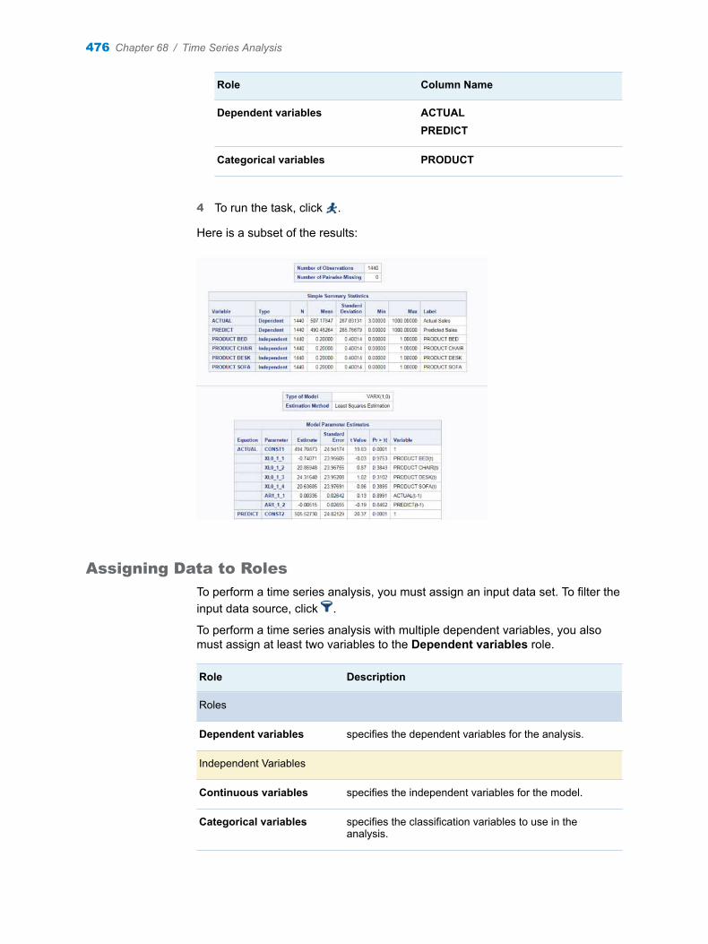
Role Column Name
Dependent variables ACTUALPREDICT
Categorical variables PRODUCT
4 To run the task, click .
Here is a subset of the results:
Assigning Data to Roles
To perform a time series analysis, you must assign an input data set. To filter the input data source, click .
To perform a time series analysis with multiple dependent variables, you also must assign at least two variables to the Dependent variables role.
Role Description
Roles
Dependent variables specifies the dependent variables for the analysis.
Independent Variables
Continuous variables specifies the independent variables for the model.
Categorical variables specifies the classification variables to use in the analysis.
476 Chapter 68 / Time Series Analysis
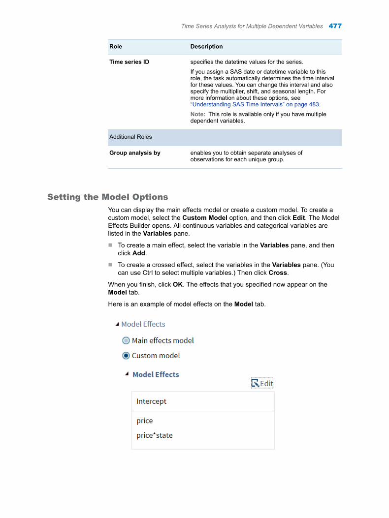
Role Description
Time series ID specifies the datetime values for the series.
If you assign a SAS date or datetime variable to this role, the task automatically determines the time interval for these values. You can change this interval and also specify the multiplier, shift, and seasonal length. For more information about these options, see “Understanding SAS Time Intervals” on page 483.
Note: This role is available only if you have multiple dependent variables.
Additional Roles
Group analysis by enables you to obtain separate analyses of observations for each unique group.
Setting the Model Options
You can display the main effects model or create a custom model. To create a custom model, select the Custom Model option, and then click Edit. The Model Effects Builder opens. All continuous variables and categorical variables are listed in the Variables pane.
n To create a main effect, select the variable in the Variables pane, and then click Add.
n To create a crossed effect, select the variables in the Variables pane. (You can use Ctrl to select multiple variables.) Then click Cross.
When you finish, click OK. The effects that you specified now appear on the Model tab.
Here is an example of model effects on the Model tab.
Time Series Analysis for Multiple Dependent Variables 477
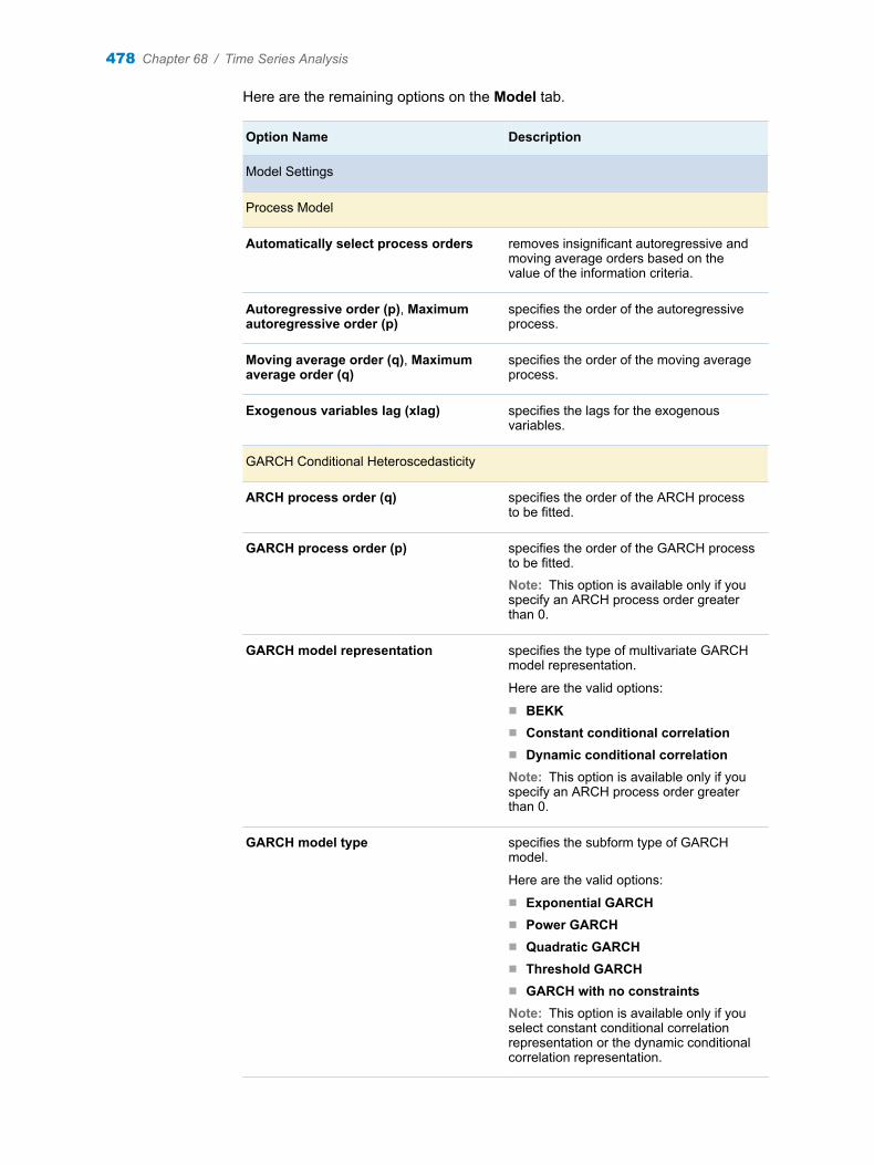
Here are the remaining options on the Model tab.
Option Name Description
Model Settings
Process Model
Automatically select process orders removes insignificant autoregressive and moving average orders based on the value of the information criteria.
Autoregressive order (p), Maximum autoregressive order (p)
specifies the order of the autoregressive process.
Moving average order (q), Maximum average order (q)
specifies the order of the moving average process.
Exogenous variables lag (xlag) specifies the lags for the exogenous variables.
GARCH Conditional Heteroscedasticity
ARCH process order (q) specifies the order of the ARCH process to be fitted.
GARCH process order (p) specifies the order of the GARCH process to be fitted.
Note: This option is available only if you specify an ARCH process order greater than 0.
GARCH model representation specifies the type of multivariate GARCH model representation.
Here are the valid options:
n BEKKn Constant conditional correlationn Dynamic conditional correlationNote: This option is available only if you specify an ARCH process order greater than 0.
GARCH model type specifies the subform type of GARCH model.
Here are the valid options:
n Exponential GARCHn Power GARCHn Quadratic GARCHn Threshold GARCHn GARCH with no constraintsNote: This option is available only if you select constant conditional correlation representation or the dynamic conditional correlation representation.
478 Chapter 68 / Time Series Analysis
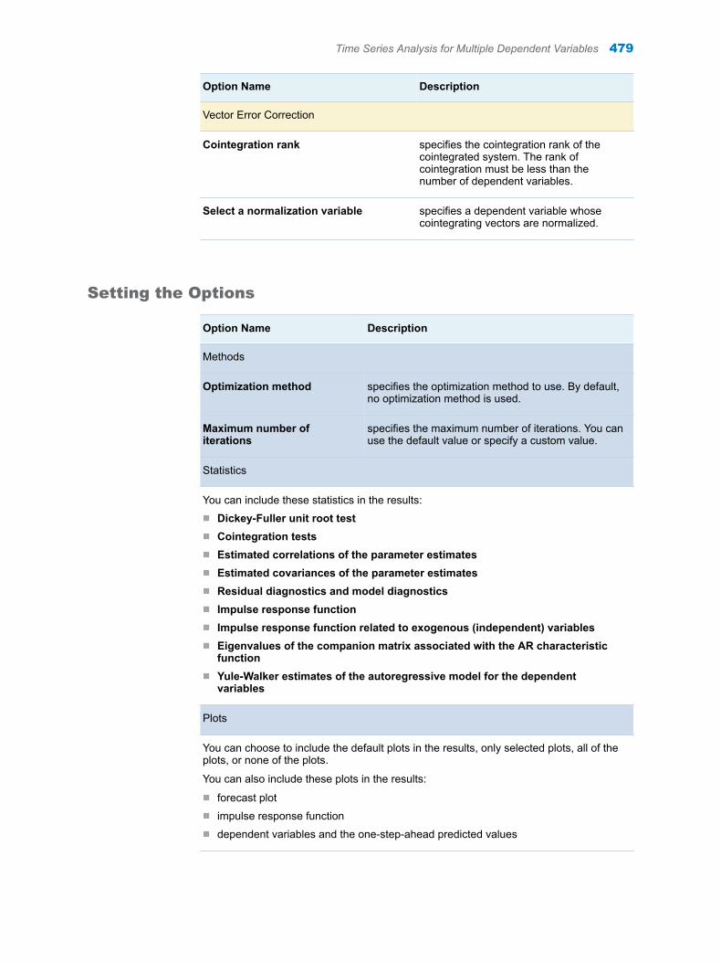
Option Name Description
Vector Error Correction
Cointegration rank specifies the cointegration rank of the cointegrated system. The rank of cointegration must be less than the number of dependent variables.
Select a normalization variable specifies a dependent variable whose cointegrating vectors are normalized.
Setting the Options
Option Name Description
Methods
Optimization method specifies the optimization method to use. By default, no optimization method is used.
Maximum number of iterations
specifies the maximum number of iterations. You can use the default value or specify a custom value.
Statistics
You can include these statistics in the results:n Dickey-Fuller unit root testn Cointegration testsn Estimated correlations of the parameter estimatesn Estimated covariances of the parameter estimatesn Residual diagnostics and model diagnosticsn Impulse response functionn Impulse response function related to exogenous (independent) variablesn Eigenvalues of the companion matrix associated with the AR characteristic
functionn Yule-Walker estimates of the autoregressive model for the dependent
variables
Plots
You can choose to include the default plots in the results, only selected plots, all of the plots, or none of the plots.
You can also include these plots in the results:
n forecast plotn impulse response functionn dependent variables and the one-step-ahead predicted values
Time Series Analysis for Multiple Dependent Variables 479

Creating an Output Data Set
You can create these output data sets:
n a data set that contains the actual values, forecast values, residuals, standard deviation of the forecasts, and the upper and lower confidence limits for the forecast
n a data set of the parameter estimates
n a data set of the residual diagnostics
480 Chapter 68 / Time Series Analysis

Part 9
Forecasting Tasks
Chapter 69Time Series Data Preparation . . . . . . . . . . . . . . . . . . . . . . . . . . . . . . . . . . . . . 483
Chapter 70Time Series Data Exploration . . . . . . . . . . . . . . . . . . . . . . . . . . . . . . . . . . . . . 491
Chapter 71Modeling and Forecasting Task . . . . . . . . . . . . . . . . . . . . . . . . . . . . . . . . . . . 501
481

482
69Time Series Data Preparation
About the Time Series Data Preparation Task . . . . . . . . . . . . . . . . . . . . . . . . . . . . . . 483
Understanding SAS Time Intervals . . . . . . . . . . . . . . . . . . . . . . . . . . . . . . . . . . . . . . . . 483
Example: Transforming the Data in the Sashelp.PriceData Data Set . . . . . . . . 486
Assigning Data to Roles . . . . . . . . . . . . . . . . . . . . . . . . . . . . . . . . . . . . . . . . . . . . . . . . . . . 487
Setting the Transformations Options . . . . . . . . . . . . . . . . . . . . . . . . . . . . . . . . . . . . . . 489
Creating the Output Data Set . . . . . . . . . . . . . . . . . . . . . . . . . . . . . . . . . . . . . . . . . . . . . . 490
About the Time Series Data Preparation Task
The Time Series Data Preparation task turns time-stamped transactional data into equally spaced time series data. This format is required for further time series analysis. This task does not require a time ID variable. If no time ID variable is specified, the observation number is the ID for the time series.
Understanding SAS Time Intervals
The Time Data Preparation task analyzes the variable assigned to the time ID role to detect the time interval of the data. SAS assumes that all of the values in the time ID variable are either date or datetime values and distinguishes between the values by their magnitude. This assumption fails if you have dates extending beyond July 21, 2196, or datetimes before January 1, 1960.
For many businesses, their time series data is equally spaced, or any two consecutive indices have the same difference between the time intervals. The following table shows an equally spaced time series with a one-year interval.
Year Number of Sales
2012 42,100
2013 45,000
483
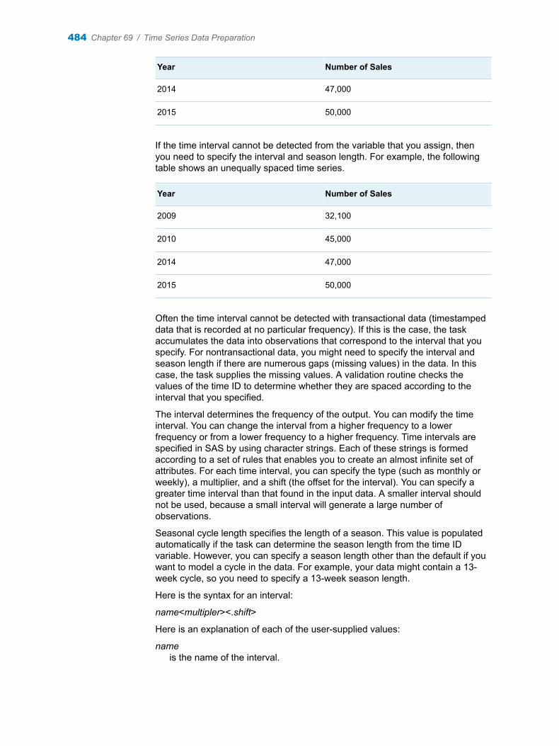
Year Number of Sales
2014 47,000
2015 50,000
If the time interval cannot be detected from the variable that you assign, then you need to specify the interval and season length. For example, the following table shows an unequally spaced time series.
Year Number of Sales
2009 32,100
2010 45,000
2014 47,000
2015 50,000
Often the time interval cannot be detected with transactional data (timestamped data that is recorded at no particular frequency). If this is the case, the task accumulates the data into observations that correspond to the interval that you specify. For nontransactional data, you might need to specify the interval and season length if there are numerous gaps (missing values) in the data. In this case, the task supplies the missing values. A validation routine checks the values of the time ID to determine whether they are spaced according to the interval that you specified.
The interval determines the frequency of the output. You can modify the time interval. You can change the interval from a higher frequency to a lower frequency or from a lower frequency to a higher frequency. Time intervals are specified in SAS by using character strings. Each of these strings is formed according to a set of rules that enables you to create an almost infinite set of attributes. For each time interval, you can specify the type (such as monthly or weekly), a multiplier, and a shift (the offset for the interval). You can specify a greater time interval than that found in the input data. A smaller interval should not be used, because a small interval will generate a large number of observations.
Seasonal cycle length specifies the length of a season. This value is populated automatically if the task can determine the season length from the time ID variable. However, you can specify a season length other than the default if you want to model a cycle in the data. For example, your data might contain a 13-week cycle, so you need to specify a 13-week season length.
Here is the syntax for an interval:
name<multipler><.shift>
Here is an explanation of each of the user-supplied values:
nameis the name of the interval.
484 Chapter 69 / Time Series Data Preparation

multiplerspecifies the multiplier of the interval. This value can be any positive number. By default, the multiplier is 1. For example, YEAR2 indicates a two-year interval.
.shiftspecifies the starting point for the interval. By default, this value is one. A value greater than 1 shifts the start to a later point within the interval. The unit for the shift depends on the interval. For example, YEAR.4 specifies a shift of four months, so the year is from April 1 through March 31 of the following year.
The examples in the following table show how the values that you specify for the interval, season length, multiplier, and shift work together.
Interval Name (in SAS code format) Default Shift Period Example
YEARm.s January 1 Months YEAR2.7 specifies an interval of every two years. Because the value for the shift is 7, the first month in the year is July.
QTRm.s January 1
April 1
July 1
October 1
Months QTR3.2 - three-month intervals starting on April 1, July 1, October 1, and January 1.
MONTHm.s First of each
month
Months MONTH2.2 - February-March, April-May, June-July, August-September, October-November, and December-January of the following year.
WEEKm.s Each Sunday Days
(1=Sunday . . .
7=Saturday)
WEEK6.3 specifies six-week intervals starting on Tuesdays.
DAYm.s Each day Days DAY3 - three-day intervals starting on Sunday.
Understanding SAS Time Intervals 485
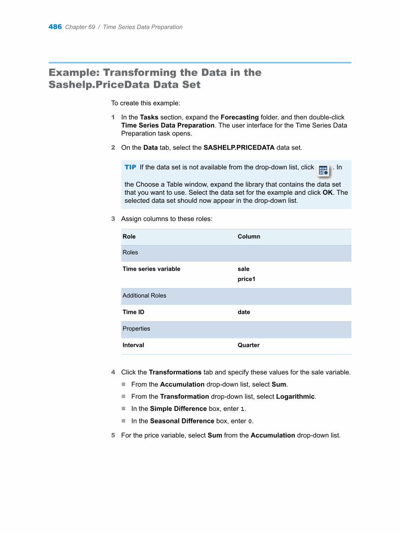
Example: Transforming the Data in the Sashelp.PriceData Data Set
To create this example:
1 In the Tasks section, expand the Forecasting folder, and then double-click Time Series Data Preparation. The user interface for the Time Series Data Preparation task opens.
2 On the Data tab, select the SASHELP.PRICEDATA data set.
TIP If the data set is not available from the drop-down list, click . In
the Choose a Table window, expand the library that contains the data set that you want to use. Select the data set for the example and click OK. The selected data set should now appear in the drop-down list.
3 Assign columns to these roles:
Role Column
Roles
Time series variable saleprice1
Additional Roles
Time ID date
Properties
Interval Quarter
4 Click the Transformations tab and specify these values for the sale variable.
n From the Accumulation drop-down list, select Sum.
n From the Transformation drop-down list, select Logarithmic.
n In the Simple Difference box, enter 1.
n In the Seasonal Difference box, enter 0.
5 For the price variable, select Sum from the Accumulation drop-down list.
486 Chapter 69 / Time Series Data Preparation

6 On the Output tab, select the Show output data check box. In the Number of observations to show box, enter 10.
7 To run the task, click .
The results show the first 10 observations in the output data set.
Assigning Data to Roles
To run the Time Series Data Preparation task, you must select an input data source. To filter the input data source, click .
You must assign a column to the Time series variable role.
Roles and Options Description
Roles
Assigning Data to Roles 487

Roles and Options Description
Time series variable lists the variables that contain timestamped data
Treatment of missing values specifies how to treat missing values in the timestamped data. You can choose from these options:n Missing valuen Average value of the accumulated
time seriesn Minimum value of the accumulated
time series n Median value of the accumulated
time series n Maximum value of the accumulated
time series n First nonmissing value of the
accumulated time series n Last nonmissing value of the
accumulated time series n The previous period’s accumulated
nonmissing value - The missing values are set to the previous accumulated nonmissing value. Missing values at the beginning of the accumulated series remain missing.
n The next period’s accumulated nonmissing value - The missing values are set to the next accumulated nonmissing value. Missing values at the end of the accumulated series remain missing.
n Numeric value specifies the value to use for the missing value.
Additional Roles
Time ID specifies the column that contains the time ID values.
Properties
Interval specifies the interval for the time ID variable. For more information about time intervals, see “Understanding SAS Time Intervals” on page 483.
Multiplier specifies the multiplier for the time interval. By default, the multiplier is 1. This value cannot be negative.
Shift specifies the shift for the time interval. By default, the shift is 1. This value cannot be negative.
488 Chapter 69 / Time Series Data Preparation
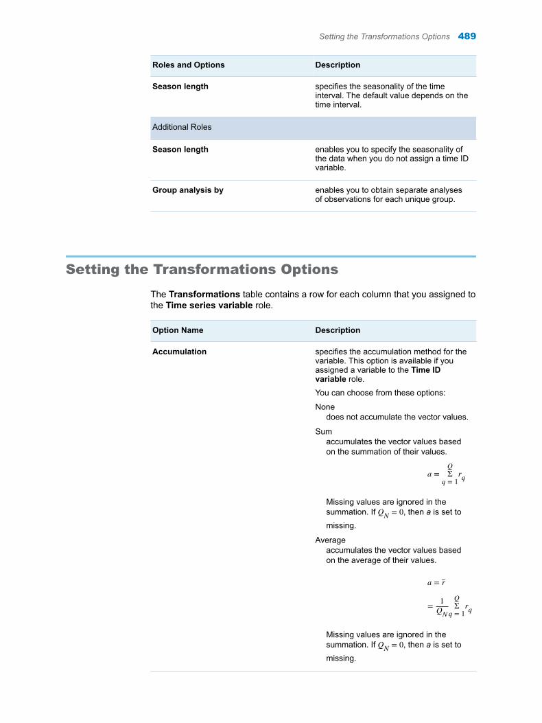
Roles and Options Description
Season length specifies the seasonality of the time interval. The default value depends on the time interval.
Additional Roles
Season length enables you to specify the seasonality of the data when you do not assign a time ID variable.
Group analysis by enables you to obtain separate analyses of observations for each unique group.
Setting the Transformations Options
The Transformations table contains a row for each column that you assigned to the Time series variable role.
Option Name Description
Accumulation specifies the accumulation method for the variable. This option is available if you assigned a variable to the Time ID variable role.
You can choose from these options:
Nonedoes not accumulate the vector values.
Sumaccumulates the vector values based on the summation of their values.
a = Σq = 1
Qrq
Missing values are ignored in the summation. If QN = 0, then a is set to missing.
Averageaccumulates the vector values based on the average of their values.
a = r
= 1QN
Σq = 1
Qrq
Missing values are ignored in the summation. If QN = 0, then a is set to missing.
Setting the Transformations Options 489
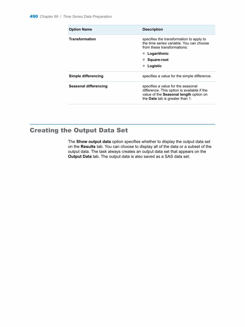
Option Name Description
Transformation specifies the transformation to apply to the time series variable. You can choose from these transformations:n Logarithmicn Square-rootn Logistic
Simple differencing specifies a value for the simple difference.
Seasonal differencing specifies a value for the seasonal difference. This option is available if the value of the Seasonal length option on the Data tab is greater than 1.
Creating the Output Data Set
The Show output data option specifies whether to display the output data set on the Results tab. You can choose to display all of the data or a subset of the output data. The task always creates an output data set that appears on the Output Data tab. The output data is also saved as a SAS data set.
490 Chapter 69 / Time Series Data Preparation
70Time Series Data Exploration
About the Time Series Exploration Task . . . . . . . . . . . . . . . . . . . . . . . . . . . . . . . . . . . 491
Example: Exploring the Sashelp.PriceData Data Set . . . . . . . . . . . . . . . . . . . . . . . 491
Assigning Data to Roles . . . . . . . . . . . . . . . . . . . . . . . . . . . . . . . . . . . . . . . . . . . . . . . . . . . 495
Setting the Analyses Options . . . . . . . . . . . . . . . . . . . . . . . . . . . . . . . . . . . . . . . . . . . . . . 496
About the Time Series Exploration Task
The Time Series Exploration task creates graphs and statistics that enable you to view and analyze your time series data.
Example: Exploring the Sashelp.PriceData Data Set
To create this example:
1 In the Tasks section, expand the Forecasting folder, and then double-click Time Series Exploration. The user interface for the Time Series Exploration task opens.
2 On the Data tab, select the SASHELP.PRICEDATA data set.
TIP If the data set is not available from the drop-down list, click . In
the Choose a Table window, expand the library that contains the data set that you want to use. Select the data set for the example and click OK. The selected data set should now appear in the drop-down list.
3 Assign columns to these roles and specify these options:
a To the Dependent variable role, assign the sale variable.
b Expand the Additional Roles heading. To the Time ID role, assign the date variable. From the Interval drop-down list, select Quarter.
491
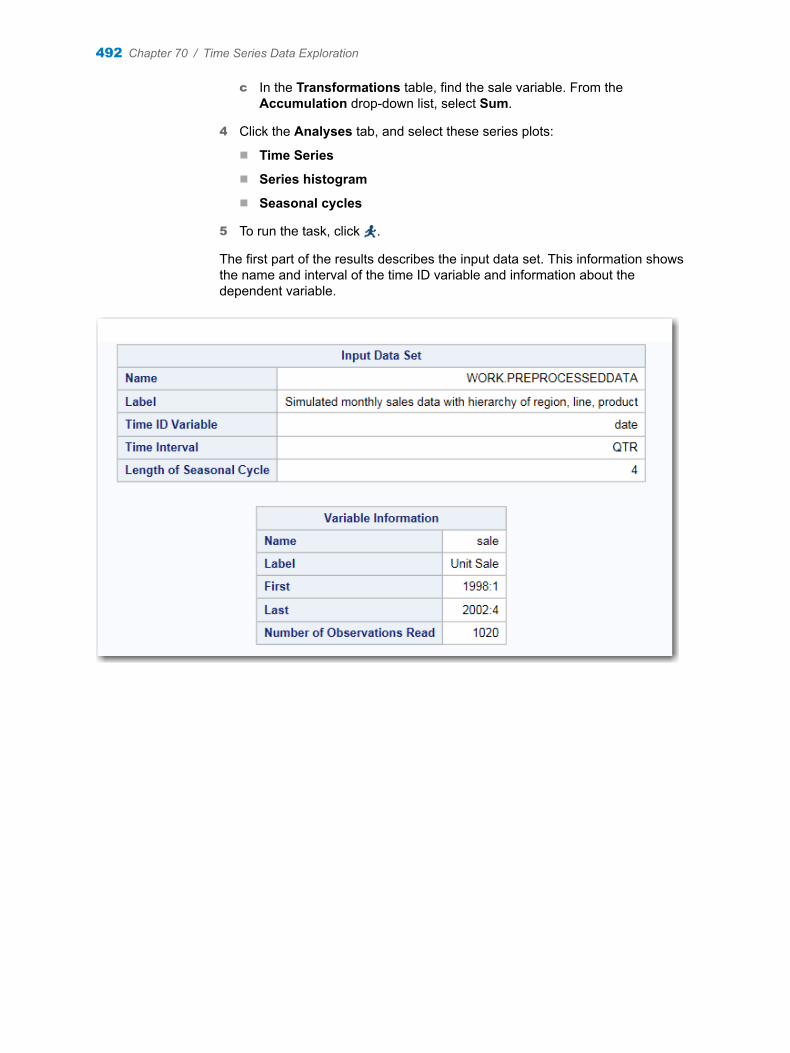
c In the Transformations table, find the sale variable. From the Accumulation drop-down list, select Sum.
4 Click the Analyses tab, and select these series plots:
n Time Series
n Series histogram
n Seasonal cycles
5 To run the task, click .
The first part of the results describes the input data set. This information shows the name and interval of the time ID variable and information about the dependent variable.
492 Chapter 70 / Time Series Data Exploration
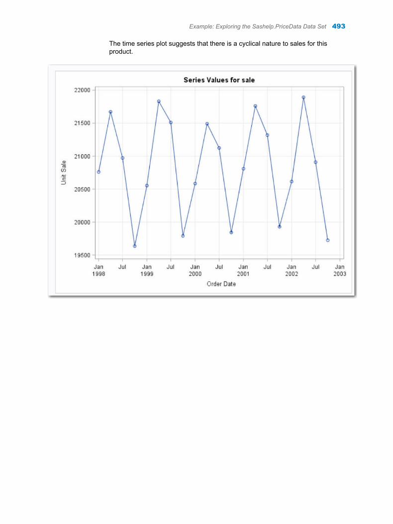
The time series plot suggests that there is a cyclical nature to sales for this product.
Example: Exploring the Sashelp.PriceData Data Set 493
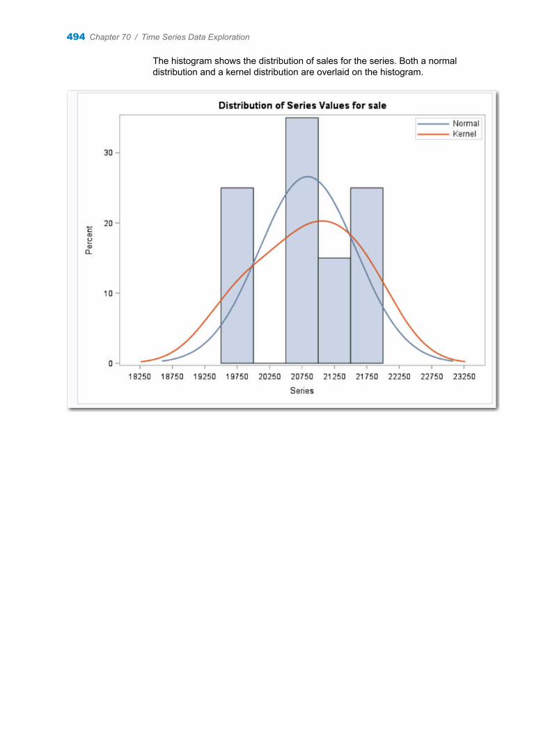
The histogram shows the distribution of sales for the series. Both a normal distribution and a kernel distribution are overlaid on the histogram.
494 Chapter 70 / Time Series Data Exploration
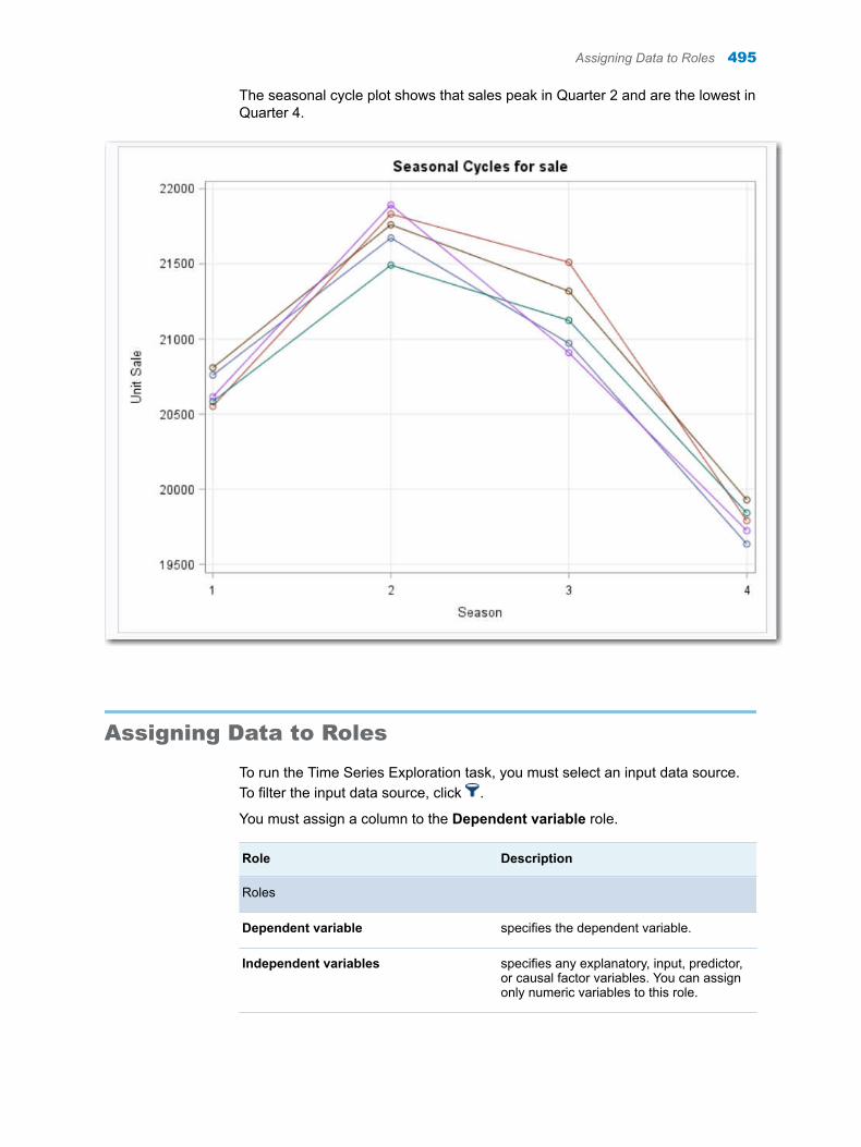
The seasonal cycle plot shows that sales peak in Quarter 2 and are the lowest in Quarter 4.
Assigning Data to Roles
To run the Time Series Exploration task, you must select an input data source. To filter the input data source, click .
You must assign a column to the Dependent variable role.
Role Description
Roles
Dependent variable specifies the dependent variable.
Independent variables specifies any explanatory, input, predictor, or causal factor variables. You can assign only numeric variables to this role.
Assigning Data to Roles 495
Role Description
Transformations specifies the transformations and simple differencing for the dependent and independent variables. If you assign a variable to the Time ID role, you can also specify an accumulation method. If the season length is greater than 1, you can specify seasonal differencing.
Additional Roles
Time ID specifies the column that contains the time ID values.
Properties
Interval specifies the interval for the time ID variable. For more information about SAS time intervals, see “Understanding SAS Time Intervals” on page 483.
Multiplier specifies the multiplier for the time interval. By default, the multiplier is 1. This value cannot be negative.
Shift specifies the shift for the time interval. By default, the shift is 1. This value cannot be negative.
Season length specifies the seasonality of the time interval. The default value depends on the time interval.
Additional Roles
Season length enables you to specify the seasonality of the data when you do not assign a time ID variable.
Group analysis by enables you to obtain separate analyses of observations for each unique group.
Setting the Analyses Options
Option Name Description
Series Plots
496 Chapter 70 / Time Series Data Exploration
Option Name Description
You can include these series plots in your results:n time series plotn series histogramn seasonal cycles
Statistics
You can include these statistics in your results:n the descriptive statistics for the accumulated time seriesn a table of the seasonal statisticsn the seasonal decomposition and adjustment tablen the trend statistics table
Autocorrelation Analysis
Perform autocorrelation analysis specifies to include an autocorrelation analysis in the results.
Select plots to display specifies the plots to display in the results. By default, the results show the autocorrelation analysis panel. However, you can select whether to include these plots in the results as well:n autocorrelation functionn normalized autocorrelation functionn partial autocorrelation functionn normalized partial autocorrelation
functionn inverse autocorrelation functionn normalized inverse autocorrelation
functionn white noise probability testn white noise probability test (log scale)
Number of lags specifies the lag values. By default, the number of lags is 0.
Cross-Correlation Analysis
Note: To perform a cross-correlation analysis, you must assign a variable to the Independent variables role.
Perform cross-correlation analysis specifies to include a cross-correlation analysis in the results.
Plots specifies the plots to include in the results. A cross-series plot is included by default. You can also include a cross-correlation function plot and a normalized cross-correlation function plot.
Setting the Analyses Options 497
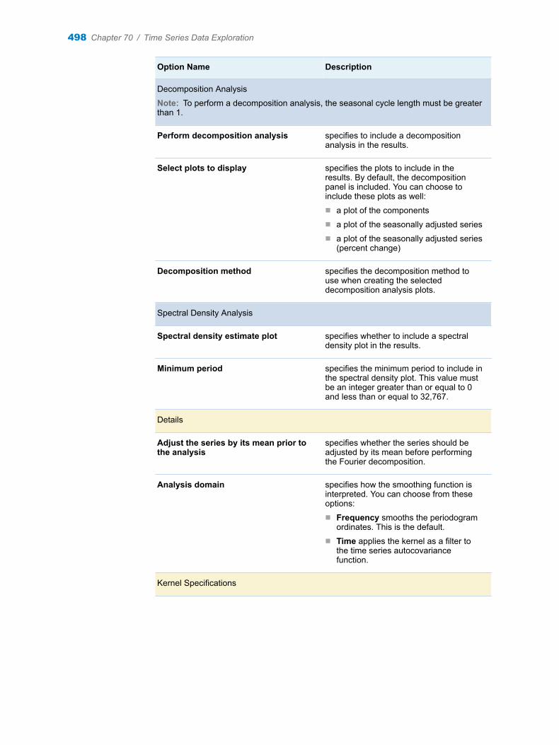
Option Name Description
Decomposition Analysis
Note: To perform a decomposition analysis, the seasonal cycle length must be greater than 1.
Perform decomposition analysis specifies to include a decomposition analysis in the results.
Select plots to display specifies the plots to include in the results. By default, the decomposition panel is included. You can choose to include these plots as well:n a plot of the componentsn a plot of the seasonally adjusted seriesn a plot of the seasonally adjusted series
(percent change)
Decomposition method specifies the decomposition method to use when creating the selected decomposition analysis plots.
Spectral Density Analysis
Spectral density estimate plot specifies whether to include a spectral density plot in the results.
Minimum period specifies the minimum period to include in the spectral density plot. This value must be an integer greater than or equal to 0 and less than or equal to 32,767.
Details
Adjust the series by its mean prior to the analysis
specifies whether the series should be adjusted by its mean before performing the Fourier decomposition.
Analysis domain specifies how the smoothing function is interpreted. You can choose from these options:n Frequency smooths the periodogram
ordinates. This is the default.n Time applies the kernel as a filter to
the time series autocovariance function.
Kernel Specifications
498 Chapter 70 / Time Series Data Exploration
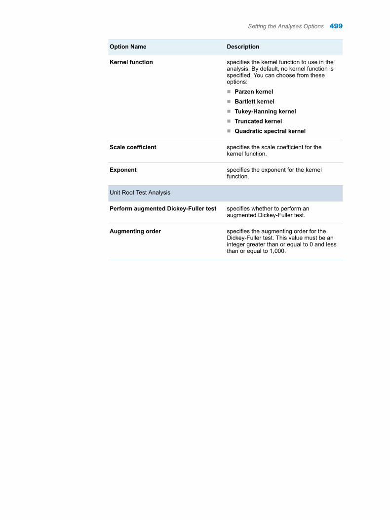
Option Name Description
Kernel function specifies the kernel function to use in the analysis. By default, no kernel function is specified. You can choose from these options:n Parzen kerneln Bartlett kerneln Tukey-Hanning kerneln Truncated kerneln Quadratic spectral kernel
Scale coefficient specifies the scale coefficient for the kernel function.
Exponent specifies the exponent for the kernel function.
Unit Root Test Analysis
Perform augmented Dickey-Fuller test specifies whether to perform an augmented Dickey-Fuller test.
Augmenting order specifies the augmenting order for the Dickey-Fuller test. This value must be an integer greater than or equal to 0 and less than or equal to 1,000.
Setting the Analyses Options 499

500 Chapter 70 / Time Series Data Exploration
71Modeling and Forecasting Task
About the Modeling and Forecasting Task . . . . . . . . . . . . . . . . . . . . . . . . . . . . . . . . . 501
Example: Creating a Random Walk Model for the SASHELP.PRICEDATA Data Set . . . . . . . . . . . . . . . . . . . . . . . . . . . . . . . . . . . . . . . . . . . . 501
Assigning Data to Roles . . . . . . . . . . . . . . . . . . . . . . . . . . . . . . . . . . . . . . . . . . . . . . . . . . . 503
Setting the Model Options . . . . . . . . . . . . . . . . . . . . . . . . . . . . . . . . . . . . . . . . . . . . . . . . . 504Random Walk . . . . . . . . . . . . . . . . . . . . . . . . . . . . . . . . . . . . . . . . . . . . . . . . . . . . . . . . . . . 505Moving Average . . . . . . . . . . . . . . . . . . . . . . . . . . . . . . . . . . . . . . . . . . . . . . . . . . . . . . . . . 505Exponential Smoothing . . . . . . . . . . . . . . . . . . . . . . . . . . . . . . . . . . . . . . . . . . . . . . . . . . 505ARIMA . . . . . . . . . . . . . . . . . . . . . . . . . . . . . . . . . . . . . . . . . . . . . . . . . . . . . . . . . . . . . . . . . 506ARIMAX . . . . . . . . . . . . . . . . . . . . . . . . . . . . . . . . . . . . . . . . . . . . . . . . . . . . . . . . . . . . . . . . 507Unobserved Components . . . . . . . . . . . . . . . . . . . . . . . . . . . . . . . . . . . . . . . . . . . . . . . . 507
Setting the Forecasting Options . . . . . . . . . . . . . . . . . . . . . . . . . . . . . . . . . . . . . . . . . . . 509
Setting the Output Options . . . . . . . . . . . . . . . . . . . . . . . . . . . . . . . . . . . . . . . . . . . . . . . . 509
About the Modeling and Forecasting Task
The Modeling and Forecasting task creates forecasting models that use your time series data. This task requires data in a valid time series format. To create this data, use the Time Series Data Preparation task before running the Modeling and Forecasting task.
Example: Creating a Random Walk Model for the SASHELP.PRICEDATA Data Set
To create this example:
1 In the Tasks section, expand the Forecasting folder, and then double-click Modeling and Forecasting. The user interface for the Modeling and Forecasting task opens.
2 On the Data tab, select the SASHELP.PRICEDATA data set.
501
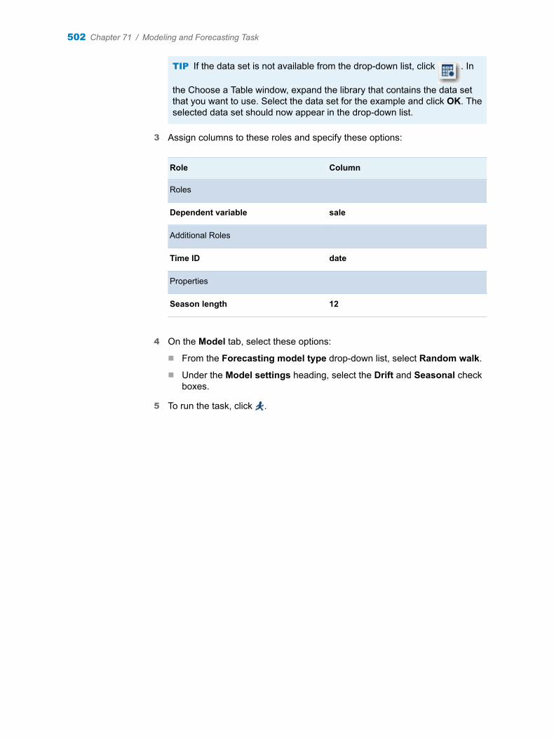
TIP If the data set is not available from the drop-down list, click . In
the Choose a Table window, expand the library that contains the data set that you want to use. Select the data set for the example and click OK. The selected data set should now appear in the drop-down list.
3 Assign columns to these roles and specify these options:
Role Column
Roles
Dependent variable sale
Additional Roles
Time ID date
Properties
Season length 12
4 On the Model tab, select these options:
n From the Forecasting model type drop-down list, select Random walk.
n Under the Model settings heading, select the Drift and Seasonal check boxes.
5 To run the task, click .
502 Chapter 71 / Modeling and Forecasting Task
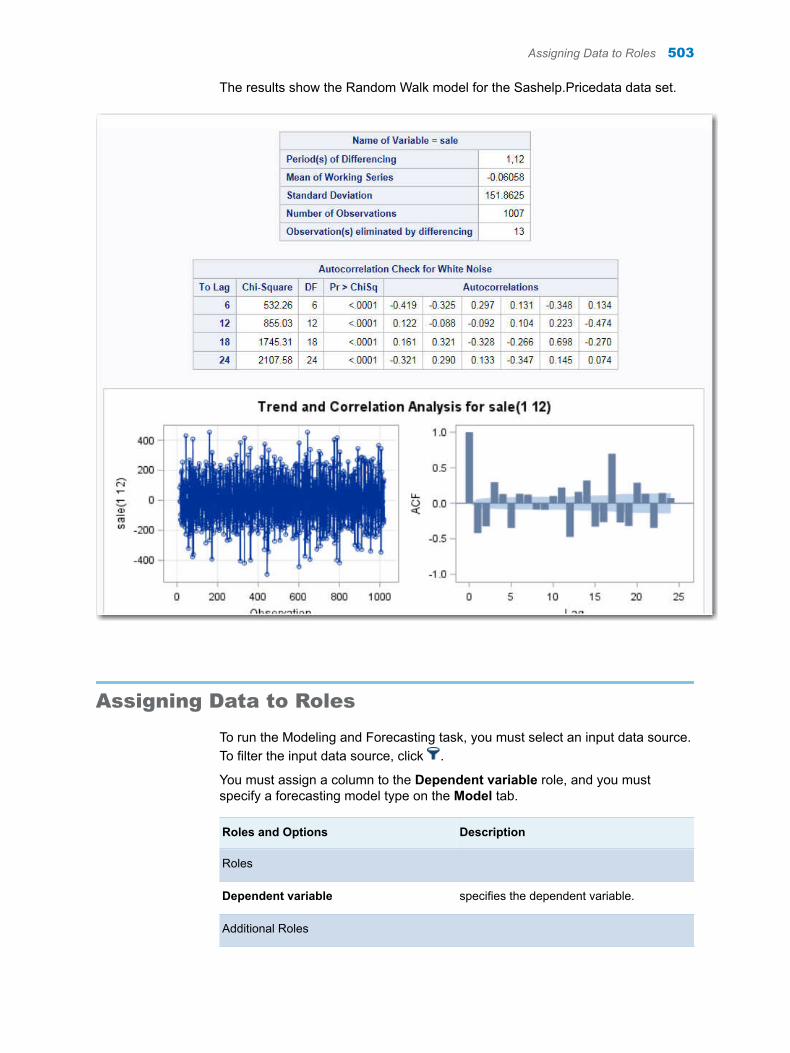
The results show the Random Walk model for the Sashelp.Pricedata data set.
Assigning Data to Roles
To run the Modeling and Forecasting task, you must select an input data source. To filter the input data source, click .
You must assign a column to the Dependent variable role, and you must specify a forecasting model type on the Model tab.
Roles and Options Description
Roles
Dependent variable specifies the dependent variable.
Additional Roles
Assigning Data to Roles 503
Roles and Options Description
Time ID specifies the column that contains the time ID values.
Properties
Interval shows the interval for the time ID variable. For more information about SAS time intervals, see “Understanding SAS Time Intervals” on page 483.
Note: This value is determined by the input data set. You cannot change this value in the Modeling and Forecasting task.
Multiplier shows the multiplier for the time interval. By default, the multiplier is 1.
Note: This value is determined by the input data set. You cannot change this value in the Modeling and Forecasting task.
Shift shows the shift for the time interval. By default, the shift is 1.
Note: This value is determined by the input data set. You cannot change this value in the Modeling and Forecasting task.
Season length specifies the seasonality of the time interval. The default value depends on the time interval.
Additional Roles
Season length enables you to specify the seasonality of the data when you do not assign a time ID variable.
Group analysis by enables you to obtain separate analyses of observations for each unique group.
Setting the Model OptionsTo use the Modeling and Forecasting task, you must select a forecasting model type. You can choose from six model types: random walk, moving average, exponential smoothing, ARIMA, ARIMAX, and unobserved components.
504 Chapter 71 / Modeling and Forecasting Task
Random Walk
To create a random walk model:
1 From the Forecasting model type drop-down list, select Random walk.
2 Select one of these types of random walk models:
n Drift creates a Random Walk model with Drift, or in ARIMA notation ARIMA(0, 1, 0).
n Trend .
n Seasonal creates a Seasonal Random Walk model, or ARIMA(0, 1, 0)(0, 1, 0)s with no intercept.
3 Under the Plots heading, select the plots to include in the results. You can choose from a variety of series plots, residual plots, and forecast plots.
Moving Average
The formula for the moving average model with width k is
yt =[yt − 1 + … + yt − k]
k + error.
In ARIMA notation, this model is ARIMA(k, 0, 0) with no intercept and with the
autoregressive parameters (AR) fixed: AR = 1k , 1
k , …, 1k .
To create a moving average model:
1 From the Forecasting model type drop-down list, select Moving average.
2 In the Window (periods) box, specify the number of periods for the moving average. This value must be an integer greater than 0 and less than 14.
3 Under the Plots heading, select the plots to include in the results. You can choose from a variety of series plots, residual plots, and forecast plots.
Exponential Smoothing
Exponential smoothing is a forecasting technique that uses exponentially declining weights to produce a weighted moving average of time series values. You can choose from several forecasting models.
To create an exponential smoothing model:
1 From the Forecasting model type drop-down list, select Exponential smoothing.
2 From the Forecasting model drop-down list, select the model that you want to use. You can choose from these models.
n Simple (single) exponential smoothing, which is the default
n Double (Brown) exponential smoothing
n Linear (Holt) exponential smoothing
Setting the Model Options 505
n Damped trend exponential smoothing
n Additive seasonal exponential smoothing
n Multiplicative seasonal exponential smoothing
n Winters multiplicative model
n Winter additive model
3 From the Transformation drop-down list, select the transformation to apply to the time series. By default, no transformation is applied. If you select the Box-Cox transformation, then you must specify a parameter value between -5 and 5 in the Box-Cox transformation parameter box.
4 From the Forecast type drop-down list, specify whether the model uses the mean forecasts or the median forecasts.
5 Under the Plots heading, select the plots to include in the results. You can choose from a variety of model plots, error plots, and forecast plots.
ARIMA
When you create an Autoregressive Integrated Moving Average (ARIMA) model, you can specify the autoregressive and moving average polynomials of an ARIMA model.
To create an ARIMA model:
1 From the Forecasting model type drop-down list, select ARIMA.
2 Under the ARIMA heading, specify the autoregressive, differencing, and moving average orders for the ARIMA model.
Here are the options for the simple ARIMA:
n Autoregressive order (p) specifies the simple autoregressive order. You can specify an integer from 0 to 13. The default value is 0.
n Differencing order (d) specifies the simple differencing order. You can specify an integer from 0 to 13. The default value is 0.
n Moving average order (q) specifies the simple moving average. You can specify an integer from 0 to 13. The default value is 0.
Here are the options for the seasonal ARIMA:
n Autoregressive order (P) specifies the seasonal autoregressive order. You can specify an integer from 0 to 5. The default value is 0.
n Differencing order (D) specifies the simple differencing order. You can specify an integer from 0 to 3. The default value is 0.
n Moving average order (Q) specifies the simple moving average. You can specify an integer from 0 to 5. The default value is 0.
3 Specify whether to include the intercept in the model. The intercept is included by default.
4 Under the Plots heading, select the plots to include in the results. You can choose from a variety of series plots, residual plots, and forecast plots.
506 Chapter 71 / Modeling and Forecasting Task
ARIMAX
When you create an Autoregressive Integrated Moving Average (ARIMA) model, you can specify the autoregressive and moving average polynomials of an ARIMA model. In an ARIMAX model, you can also include independent variables in the model.
To create an ARIMAX model:
1 From the Forecasting model type drop-down list, select ARIMAX.
2 Under the ARIMA heading, specify the autoregressive, differencing, and moving average orders for the ARIMA model.
Here are the options for the simple ARIMA:
n Autoregressive order (p) specifies the simple autoregressive order. You can specify an integer from 0 to 13. The default value is 0.
n Differencing order (d) specifies the simple differencing order. You can specify an integer from 0 to 13. The default value is 0.
n Moving average order (q) specifies the simple moving average. You can specify an integer from 0 to 13. The default value is 0.
Here are the options for the seasonal ARIMA:
n Autoregressive order (P) specifies the seasonal autoregressive order. You can specify an integer from 0 to 5. The default value is 0.
n Differencing order (D) specifies the simple differencing order. You can specify an integer from 0 to 3. The default value is 0.
n Moving average order (Q) specifies the simple moving average. You can specify an integer from 0 to 5. The default value is 0.
3 In the Independent variables role, assign the variables from the input data set that you want to include in the model.
4 Specify whether to include the intercept in the model. The intercept is included by default.
5 Under the Plots heading, select the plots to include in the results. You can choose from a variety of series plots, residual plots, and forecast plots.
Unobserved Components
To create an unobserved components model:
1 From the Forecasting model type drop-down list, select Unobserved components.
2 (Optional) To include independent variables in the model, expand the Regression Effects heading and select the Include independent variables check box. Assign the variables that you want to include in the model to the Independent variables role.
3 To include an irregular component, expand the Irregular Component heading and select the Include an irregular component check box. An irregular component is included by default.
Setting the Model Options 507
The irregular component corresponds to the overall random error in the model. The initial variance is the value used as the initial value during the parameter estimation process. To change this value, select Specify variance and enter a different value. To keep this value as your initial variance, select Fix variance value.
4 To include a trend component, expand the Trend Component heading. The level component and the slope component combine to define the trend component for the model. If you specify both a level and slope component, then a locally linear trend is obtained. If you omit the slope component, then a local level is used.
a To include a level component in the model, select the Include a level component check box. (The level component is included by default.) Then you can specify whether to change the initial variance (which is 0 by default) and whether to check for level breaks.
b To include a slope component in the model, select the Include a slope component check box. Then you can specify whether to change the initial variance (which is 0 by default).
5 (Optional) To include a seasonal component, the season length must be greater than one. Expand the Seasonal Component heading and select the Include a seasonal component check box. Specify the type of seasonal component. A seasonal component can be one of two types: dummy or trigonometric. You can also specify whether to change the initial variance (which is 0 by default).
6 (Optional) To include a cycle component, expand the Cycle Component heading and select the Include a cycle component check box. You can specify these options:
n To specify an initial cycle period to use during the parameter estimation process, select the Specify cycle period check box. Then specify the initial value in the box. This value must be an integer greater than 2. By default, the initial value is 3.
n To specify an initial damping factor to use during the parameter estimation process, select the Specify damping factor check box, and then specify the initial value in the box. You can specify any value between 0 and 1 (excluding 0 but including 1). By default, the initial value is 0.01.
n To specify an initial value for the disturbance variance parameter that the task uses during the parameter estimation process, select the Specify variance check box. Then specify the initial value in the box. This value must be greater than or equal to 0. By default, the initial value is 0.
7 Under the Plots heading, select the plots to include in the results. You can choose from a variety of residual plots, smoothed component estimates, filtered component estimates, and series decomposition and forecast plots.
508 Chapter 71 / Modeling and Forecasting Task
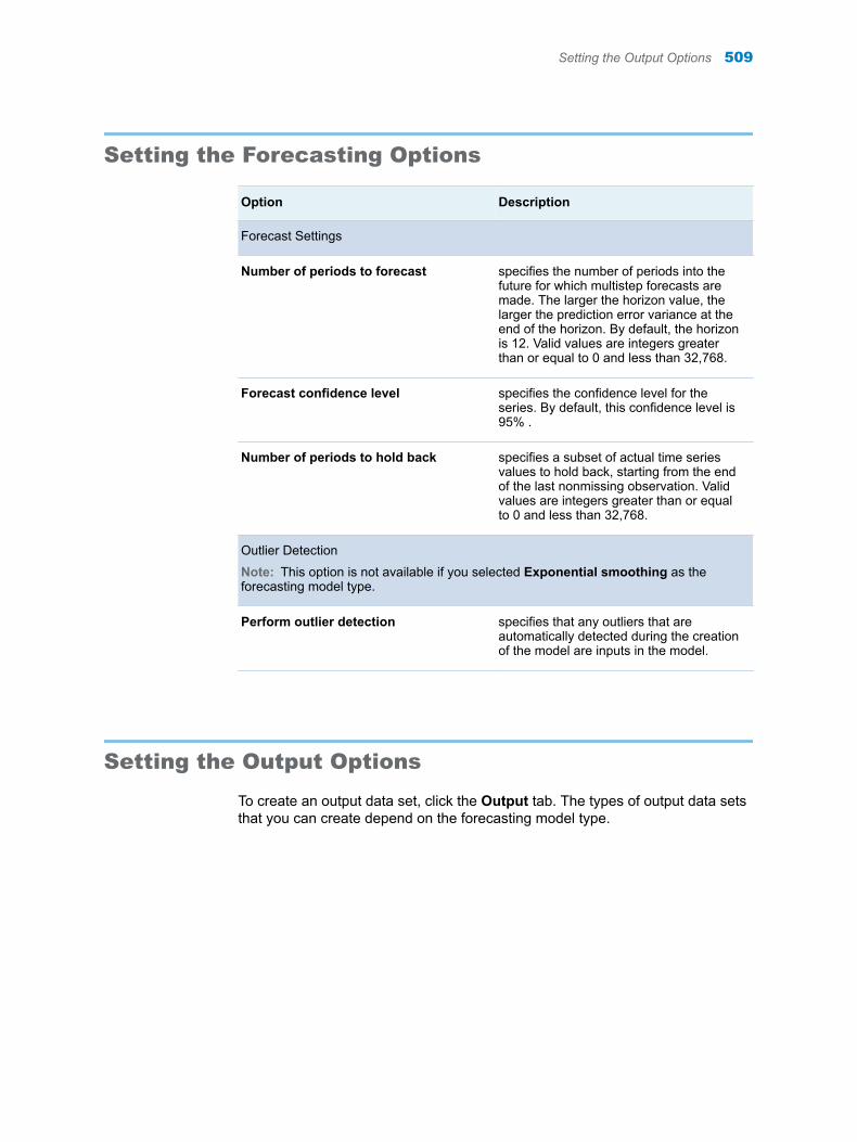
Setting the Forecasting Options
Option Description
Forecast Settings
Number of periods to forecast specifies the number of periods into the future for which multistep forecasts are made. The larger the horizon value, the larger the prediction error variance at the end of the horizon. By default, the horizon is 12. Valid values are integers greater than or equal to 0 and less than 32,768.
Forecast confidence level specifies the confidence level for the series. By default, this confidence level is 95% .
Number of periods to hold back specifies a subset of actual time series values to hold back, starting from the end of the last nonmissing observation. Valid values are integers greater than or equal to 0 and less than 32,768.
Outlier Detection
Note: This option is not available if you selected Exponential smoothing as the forecasting model type.
Perform outlier detection specifies that any outliers that are automatically detected during the creation of the model are inputs in the model.
Setting the Output Options
To create an output data set, click the Output tab. The types of output data sets that you can create depend on the forecasting model type.
Setting the Output Options 509

510 Chapter 71 / Modeling and Forecasting Task

Part 10
Statistical Process Control
Chapter 72Control Charts . . . . . . . . . . . . . . . . . . . . . . . . . . . . . . . . . . . . . . . . . . . . . . . . . . 513
Chapter 73Capability Analysis . . . . . . . . . . . . . . . . . . . . . . . . . . . . . . . . . . . . . . . . . . . . . . 527
Chapter 74Pareto Analysis . . . . . . . . . . . . . . . . . . . . . . . . . . . . . . . . . . . . . . . . . . . . . . . . . 533
Chapter 75Analysis of Means . . . . . . . . . . . . . . . . . . . . . . . . . . . . . . . . . . . . . . . . . . . . . . . 537
511

512
72Control Charts
About the Control Charts Task . . . . . . . . . . . . . . . . . . . . . . . . . . . . . . . . . . . . . . . . . . . . . 513Mean and Range Chart . . . . . . . . . . . . . . . . . . . . . . . . . . . . . . . . . . . . . . . . . . . . . . . . . . 513Mean and Standard Deviation Chart . . . . . . . . . . . . . . . . . . . . . . . . . . . . . . . . . . . . . . 514Mean with Box-and-Whisker Plot . . . . . . . . . . . . . . . . . . . . . . . . . . . . . . . . . . . . . . . . . 515Individual Measurements . . . . . . . . . . . . . . . . . . . . . . . . . . . . . . . . . . . . . . . . . . . . . . . . 516Median and Range Chart . . . . . . . . . . . . . . . . . . . . . . . . . . . . . . . . . . . . . . . . . . . . . . . . 517p Charts . . . . . . . . . . . . . . . . . . . . . . . . . . . . . . . . . . . . . . . . . . . . . . . . . . . . . . . . . . . . . . . . 518np Charts . . . . . . . . . . . . . . . . . . . . . . . . . . . . . . . . . . . . . . . . . . . . . . . . . . . . . . . . . . . . . . . 519c Chart . . . . . . . . . . . . . . . . . . . . . . . . . . . . . . . . . . . . . . . . . . . . . . . . . . . . . . . . . . . . . . . . . 520u Chart . . . . . . . . . . . . . . . . . . . . . . . . . . . . . . . . . . . . . . . . . . . . . . . . . . . . . . . . . . . . . . . . . 521
Example: Determine the Mean and Range for the Diameters of Wafers . . . . . 522
Assigning Data to Roles . . . . . . . . . . . . . . . . . . . . . . . . . . . . . . . . . . . . . . . . . . . . . . . . . . . 524
Setting Options . . . . . . . . . . . . . . . . . . . . . . . . . . . . . . . . . . . . . . . . . . . . . . . . . . . . . . . . . . . . 525
Setting the Output Options . . . . . . . . . . . . . . . . . . . . . . . . . . . . . . . . . . . . . . . . . . . . . . . . 526
About the Control Charts TaskThe Control Charts task creates Shewhart control charts for deciding whether a process is in a state of statistical control. Using the Control Charts task, you can create these types of charts.
Mean and Range Chart
The Mean and Range chart displays the subgroup means and the subgroup ranges. These charts are useful for analyzing the central tendency and the variability of a process.
Suppose that in the manufacture of silicon wafers, batches of five wafers are sampled, and their diameters are measured in millimeters. The measurements for 25 batches are stored in a SAS data set, which is used to create the mean and range charts. Each point on the mean chart represents the average (mean) of the measurements for a particular batch. Each point on the range chart represents the range of the measurements for a particular batch. If all the points fall within the control limits, you can conclude that the process is in statistical control.
513
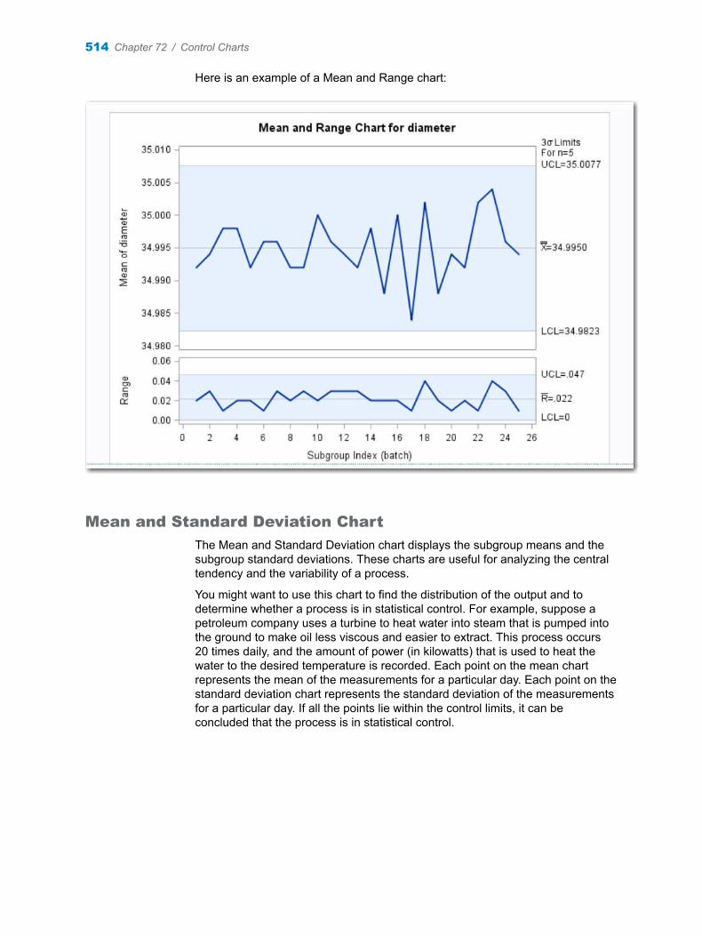
Here is an example of a Mean and Range chart:
Mean and Standard Deviation Chart
The Mean and Standard Deviation chart displays the subgroup means and the subgroup standard deviations. These charts are useful for analyzing the central tendency and the variability of a process.
You might want to use this chart to find the distribution of the output and to determine whether a process is in statistical control. For example, suppose a petroleum company uses a turbine to heat water into steam that is pumped into the ground to make oil less viscous and easier to extract. This process occurs 20 times daily, and the amount of power (in kilowatts) that is used to heat the water to the desired temperature is recorded. Each point on the mean chart represents the mean of the measurements for a particular day. Each point on the standard deviation chart represents the standard deviation of the measurements for a particular day. If all the points lie within the control limits, it can be concluded that the process is in statistical control.
514 Chapter 72 / Control Charts
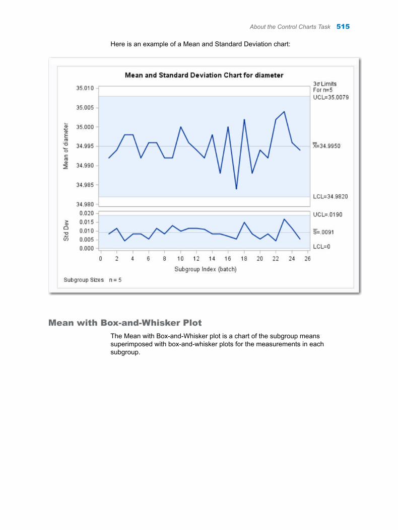
Here is an example of a Mean and Standard Deviation chart:
Mean with Box-and-Whisker Plot
The Mean with Box-and-Whisker plot is a chart of the subgroup means superimposed with box-and-whisker plots for the measurements in each subgroup.
About the Control Charts Task 515
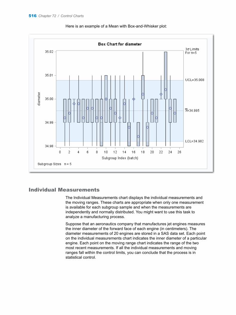
Here is an example of a Mean with Box-and-Whisker plot:
Individual Measurements
The Individual Measurements chart displays the individual measurements and the moving ranges. These charts are appropriate when only one measurement is available for each subgroup sample and when the measurements are independently and normally distributed. You might want to use this task to analyze a manufacturing process.
Suppose that an aeronautics company that manufactures jet engines measures the inner diameter of the forward face of each engine (in centimeters). The diameter measurements of 20 engines are stored in a SAS data set. Each point on the individual measurements chart indicates the inner diameter of a particular engine. Each point on the moving range chart indicates the range of the two most recent measurements. If all the individual measurements and moving ranges fall within the control limits, you can conclude that the process is in statistical control.
516 Chapter 72 / Control Charts
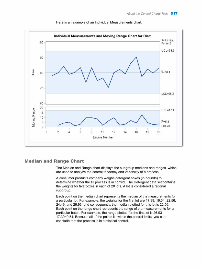
Here is an example of an Individual Measurements chart:
Median and Range Chart
The Median and Range chart displays the subgroup medians and ranges, which are used to analyze the central tendency and variability of a process.
A consumer products company weighs detergent boxes (in pounds) to determine whether the fill process is in control. The Detergent data set contains the weights for five boxes in each of 28 lots. A lot is considered a rational subgroup.
Each point on the median chart represents the median of the measurements for a particular lot. For example, the weights for the first lot are 17.39, 19.34, 22.56, 24.49, and 26.93, and consequently, the median plotted for this lot is 22.56. Each point on the range chart represents the range of the measurements for a particular batch. For example, the range plotted for the first lot is 26.93–17.39=9.54. Because all of the points lie within the control limits, you can conclude that the process is in statistical control.
About the Control Charts Task 517
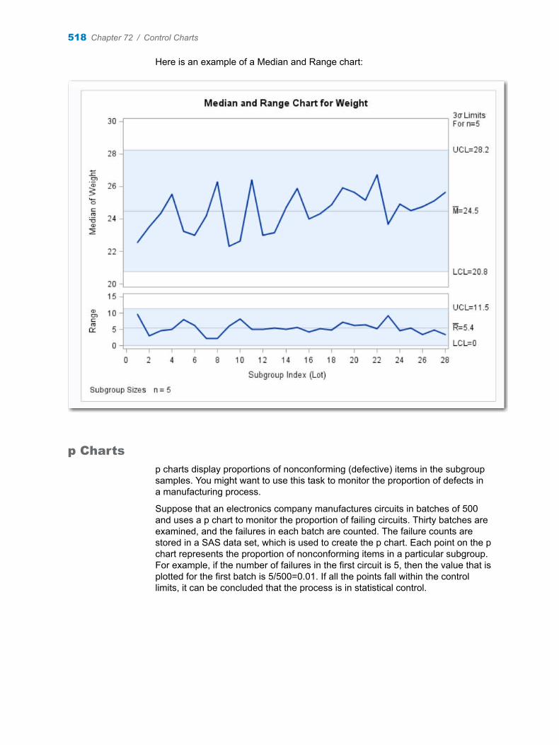
Here is an example of a Median and Range chart:
p Charts
p charts display proportions of nonconforming (defective) items in the subgroup samples. You might want to use this task to monitor the proportion of defects in a manufacturing process.
Suppose that an electronics company manufactures circuits in batches of 500 and uses a p chart to monitor the proportion of failing circuits. Thirty batches are examined, and the failures in each batch are counted. The failure counts are stored in a SAS data set, which is used to create the p chart. Each point on the p chart represents the proportion of nonconforming items in a particular subgroup. For example, if the number of failures in the first circuit is 5, then the value that is plotted for the first batch is 5/500=0.01. If all the points fall within the control limits, it can be concluded that the process is in statistical control.
518 Chapter 72 / Control Charts
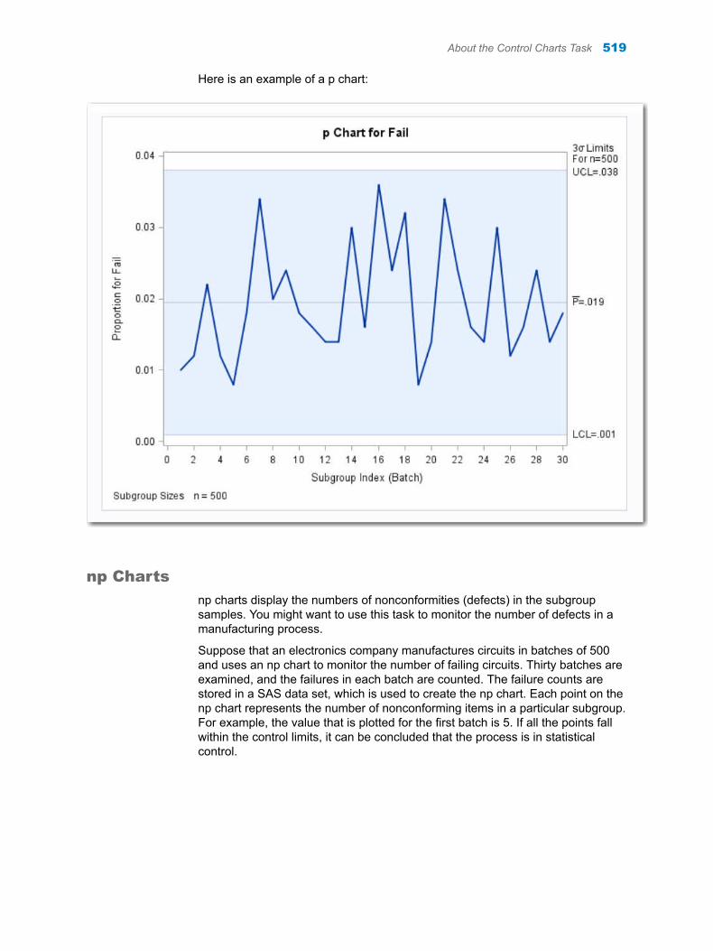
Here is an example of a p chart:
np Charts
np charts display the numbers of nonconformities (defects) in the subgroup samples. You might want to use this task to monitor the number of defects in a manufacturing process.
Suppose that an electronics company manufactures circuits in batches of 500 and uses an np chart to monitor the number of failing circuits. Thirty batches are examined, and the failures in each batch are counted. The failure counts are stored in a SAS data set, which is used to create the np chart. Each point on the np chart represents the number of nonconforming items in a particular subgroup. For example, the value that is plotted for the first batch is 5. If all the points fall within the control limits, it can be concluded that the process is in statistical control.
About the Control Charts Task 519
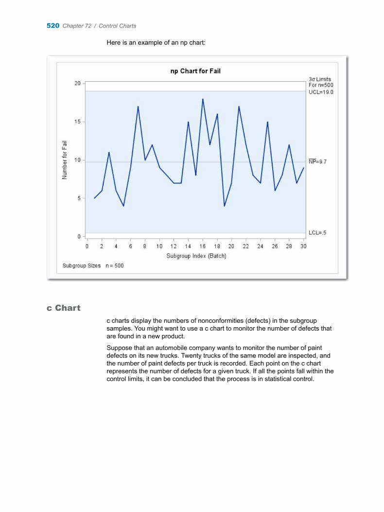
Here is an example of an np chart:
c Chart
c charts display the numbers of nonconformities (defects) in the subgroup samples. You might want to use a c chart to monitor the number of defects that are found in a new product.
Suppose that an automobile company wants to monitor the number of paint defects on its new trucks. Twenty trucks of the same model are inspected, and the number of paint defects per truck is recorded. Each point on the c chart represents the number of defects for a given truck. If all the points fall within the control limits, it can be concluded that the process is in statistical control.
520 Chapter 72 / Control Charts
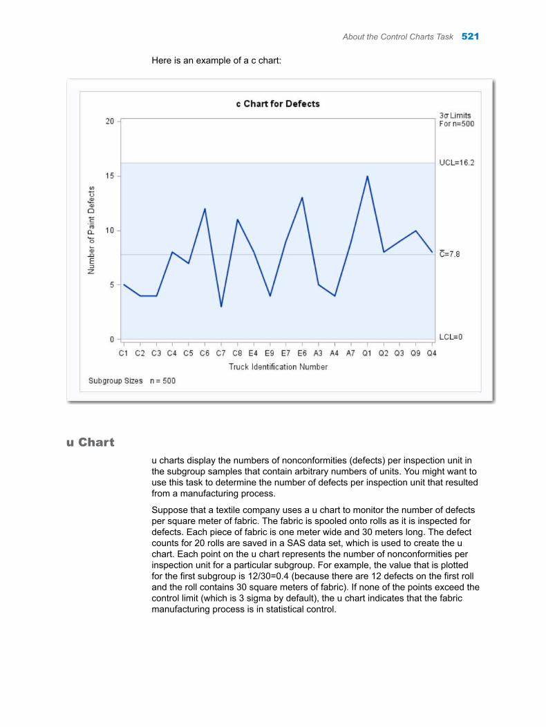
Here is an example of a c chart:
u Chart
u charts display the numbers of nonconformities (defects) per inspection unit in the subgroup samples that contain arbitrary numbers of units. You might want to use this task to determine the number of defects per inspection unit that resulted from a manufacturing process.
Suppose that a textile company uses a u chart to monitor the number of defects per square meter of fabric. The fabric is spooled onto rolls as it is inspected for defects. Each piece of fabric is one meter wide and 30 meters long. The defect counts for 20 rolls are saved in a SAS data set, which is used to create the u chart. Each point on the u chart represents the number of nonconformities per inspection unit for a particular subgroup. For example, the value that is plotted for the first subgroup is 12/30=0.4 (because there are 12 defects on the first roll and the roll contains 30 square meters of fabric). If none of the points exceed the control limit (which is 3 sigma by default), the u chart indicates that the fabric manufacturing process is in statistical control.
About the Control Charts Task 521
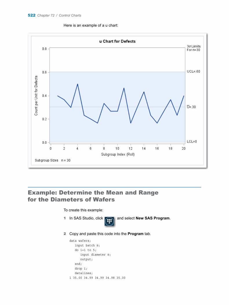
Here is an example of a u chart:
Example: Determine the Mean and Range for the Diameters of Wafers
To create this example:
1 In SAS Studio, click and select New SAS Program.
2 Copy and paste this code into the Program tab.
data wafers; input batch @; do i=1 to 5; input diameter @; output; end; drop i; datalines;1 35.00 34.99 34.99 34.98 35.00
522 Chapter 72 / Control Charts
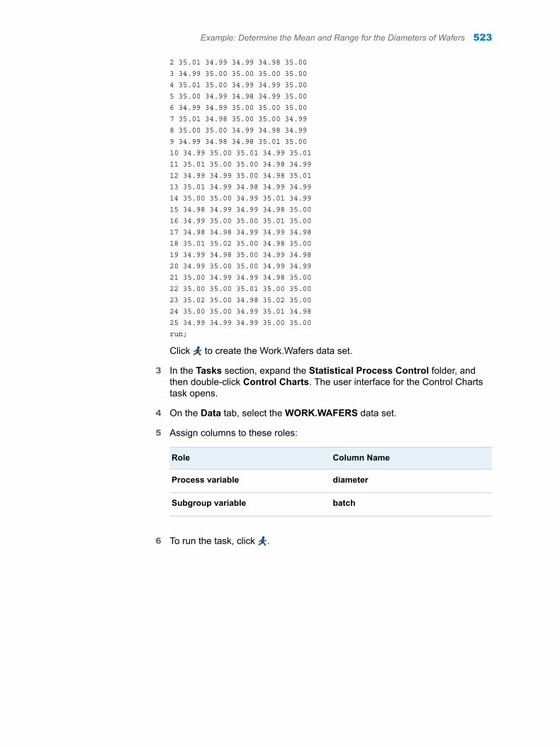
2 35.01 34.99 34.99 34.98 35.003 34.99 35.00 35.00 35.00 35.004 35.01 35.00 34.99 34.99 35.005 35.00 34.99 34.98 34.99 35.006 34.99 34.99 35.00 35.00 35.007 35.01 34.98 35.00 35.00 34.998 35.00 35.00 34.99 34.98 34.999 34.99 34.98 34.98 35.01 35.0010 34.99 35.00 35.01 34.99 35.0111 35.01 35.00 35.00 34.98 34.9912 34.99 34.99 35.00 34.98 35.0113 35.01 34.99 34.98 34.99 34.9914 35.00 35.00 34.99 35.01 34.9915 34.98 34.99 34.99 34.98 35.0016 34.99 35.00 35.00 35.01 35.0017 34.98 34.98 34.99 34.99 34.9818 35.01 35.02 35.00 34.98 35.0019 34.99 34.98 35.00 34.99 34.9820 34.99 35.00 35.00 34.99 34.9921 35.00 34.99 34.99 34.98 35.0022 35.00 35.00 35.01 35.00 35.0023 35.02 35.00 34.98 35.02 35.0024 35.00 35.00 34.99 35.01 34.9825 34.99 34.99 34.99 35.00 35.00run;
Click to create the Work.Wafers data set.
3 In the Tasks section, expand the Statistical Process Control folder, and then double-click Control Charts. The user interface for the Control Charts task opens.
4 On the Data tab, select the WORK.WAFERS data set.
5 Assign columns to these roles:
Role Column Name
Process variable diameter
Subgroup variable batch
6 To run the task, click .
Example: Determine the Mean and Range for the Diameters of Wafers 523
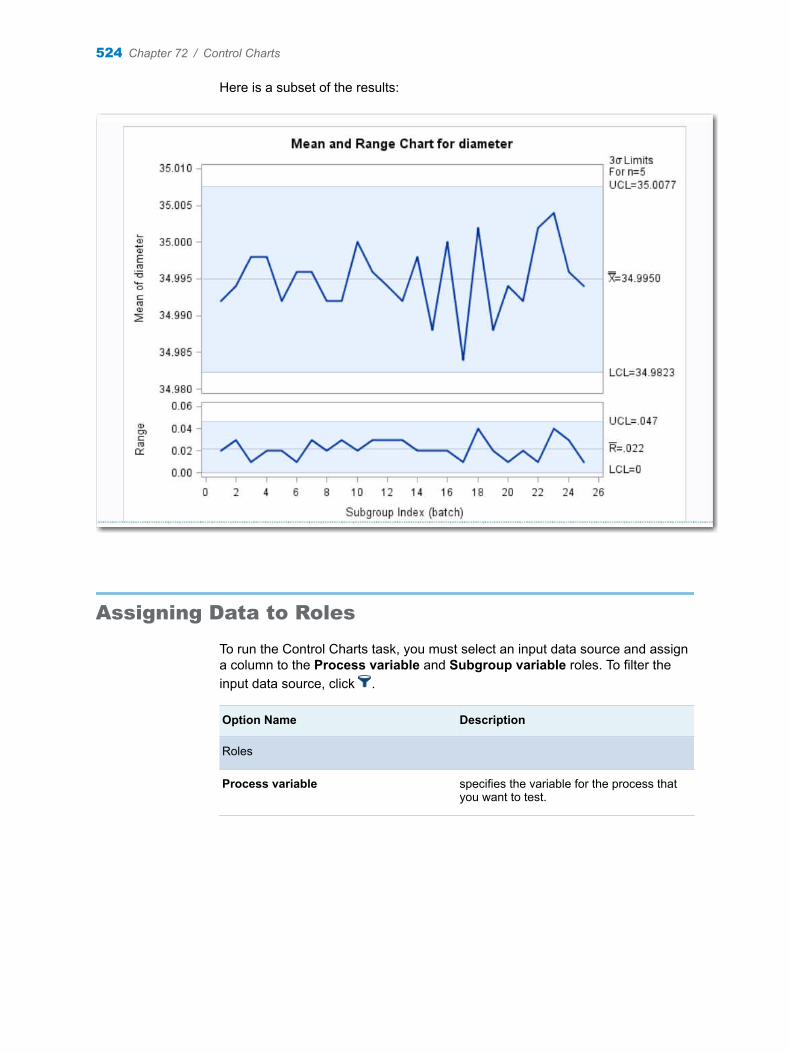
Here is a subset of the results:
Assigning Data to Roles
To run the Control Charts task, you must select an input data source and assign a column to the Process variable and Subgroup variable roles. To filter the input data source, click .
Option Name Description
Roles
Process variable specifies the variable for the process that you want to test.
524 Chapter 72 / Control Charts
Option Name Description
Subgroup variable specifies the variable that identifies the subgroups in the data. The values of this variable indicate how the observations in the input data set are arranged into rational subgroups.
Here are some examples of the subgroup values:
n indices that give the order in which the subgroup samples were collected
n the dates or times at which the subgroup samples were collected
n the labels that uniquely identify the subgroup samples
Chart type specifies the type of control chart to create. For more information about the different chart types, see “About the Control Charts Task” on page 513.
Additional Roles
Group analysis by enables you to obtain separate analyses of observations for each unique group.
Setting Options
Option Name Description
Control Limits
Method specifies whether to compute the control limits by using the current input data set or to compute the control limits from a different data set.n If you use the current input data, you can set the
Limits based on option. n If you want to compute the data from a different
data set, select Use stored limits. Then select the data set to use. The data set that you select must be a LIMITS= data set. For more information about the variables that are required in a LIMITS= data set, see the procedure documentation for the chart that you are creating. In the Control Charts task, you can create this data set by selecting the Save control limits check box on the Output tab.
Limits based on specifies the width of the control limits as a multiple of the standard error (sigma) of the summary subgroup statistic that is plotted on the chart. The width must be positive. The default multiple is 3.
Setting Options 525
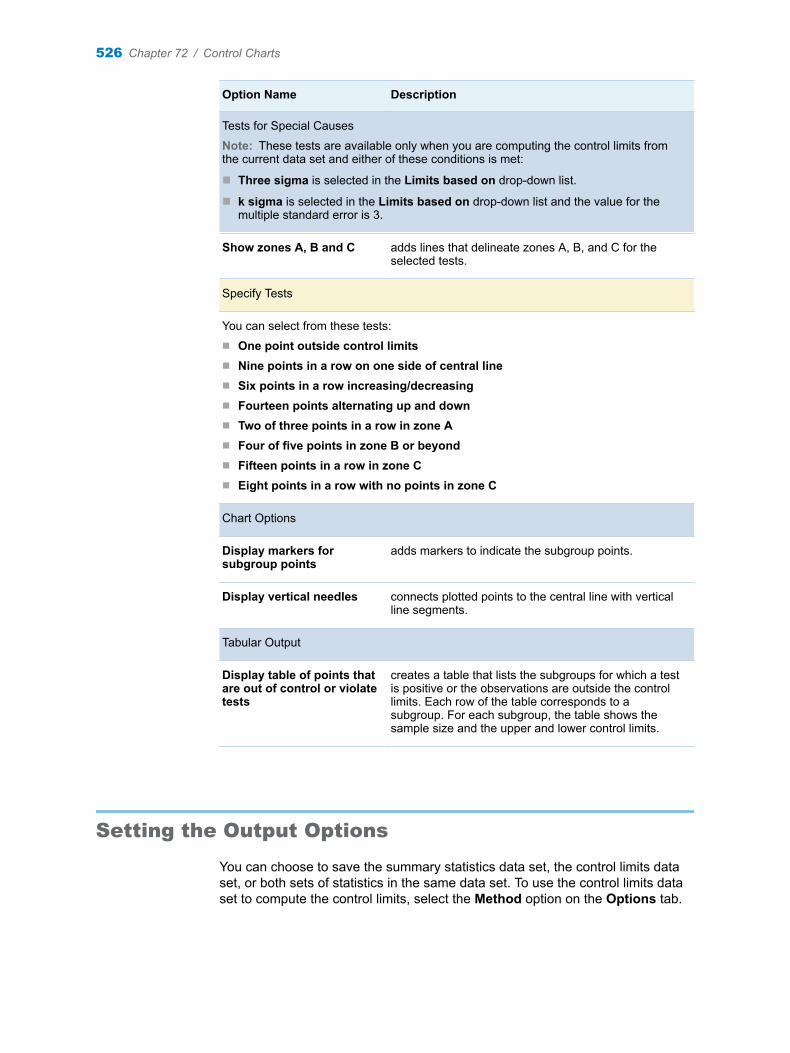
Option Name Description
Tests for Special Causes
Note: These tests are available only when you are computing the control limits from the current data set and either of these conditions is met:
n Three sigma is selected in the Limits based on drop-down list.
n k sigma is selected in the Limits based on drop-down list and the value for the multiple standard error is 3.
Show zones A, B and C adds lines that delineate zones A, B, and C for the selected tests.
Specify Tests
You can select from these tests:n One point outside control limitsn Nine points in a row on one side of central linen Six points in a row increasing/decreasingn Fourteen points alternating up and downn Two of three points in a row in zone An Four of five points in zone B or beyondn Fifteen points in a row in zone Cn Eight points in a row with no points in zone C
Chart Options
Display markers for subgroup points
adds markers to indicate the subgroup points.
Display vertical needles connects plotted points to the central line with vertical line segments.
Tabular Output
Display table of points that are out of control or violate tests
creates a table that lists the subgroups for which a test is positive or the observations are outside the control limits. Each row of the table corresponds to a subgroup. For each subgroup, the table shows the sample size and the upper and lower control limits.
Setting the Output Options
You can choose to save the summary statistics data set, the control limits data set, or both sets of statistics in the same data set. To use the control limits data set to compute the control limits, select the Method option on the Options tab.
526 Chapter 72 / Control Charts

73Capability Analysis
About the Capability Analysis Task . . . . . . . . . . . . . . . . . . . . . . . . . . . . . . . . . . . . . . . . 527
Example: Analysis of Plating Thickness . . . . . . . . . . . . . . . . . . . . . . . . . . . . . . . . . . . 528
Assigning Data to Roles . . . . . . . . . . . . . . . . . . . . . . . . . . . . . . . . . . . . . . . . . . . . . . . . . . . 530
Setting Options . . . . . . . . . . . . . . . . . . . . . . . . . . . . . . . . . . . . . . . . . . . . . . . . . . . . . . . . . . . . 531
Setting the Output Options . . . . . . . . . . . . . . . . . . . . . . . . . . . . . . . . . . . . . . . . . . . . . . . . 531
About the Capability Analysis Task
Capability analysis compares the distribution of a process to its specification limits. When you run the Capability Analysis task, the output includes a variety of statistics for summarizing the data distribution of the process variable. Examples of statistics are sample moments, basic statistical measures, and quantiles.
When you add specification limits, the output includes statistics such as percents of measurements within and outside the specification limits and process capability indices.
You can plot the results by using a histogram, a probability plot, and a quantile-quantile plot.
n Histograms are typically used in process capability analysis to compare the distribution of measurements from an in-control process to its specification limits.
n A probability plot compares ordered values of a variable with percentiles of a specified theoretical distribution such as the normal. If the data distribution matches the theoretical distribution, the points on the plot form a linear pattern. Thus, you can use a probability plot to determine how well a theoretical distribution models a set of measurements.
n A quantile-quantile plot (Q-Q plot) compares ordered values of a variable with quantiles of a specified theoretical distribution such as the normal. If the data distribution matches the theoretical distribution, the points on the plot form a linear pattern. Thus, you can use a Q-Q plot to determine how well a theoretical distribution models a set of measurements.
527
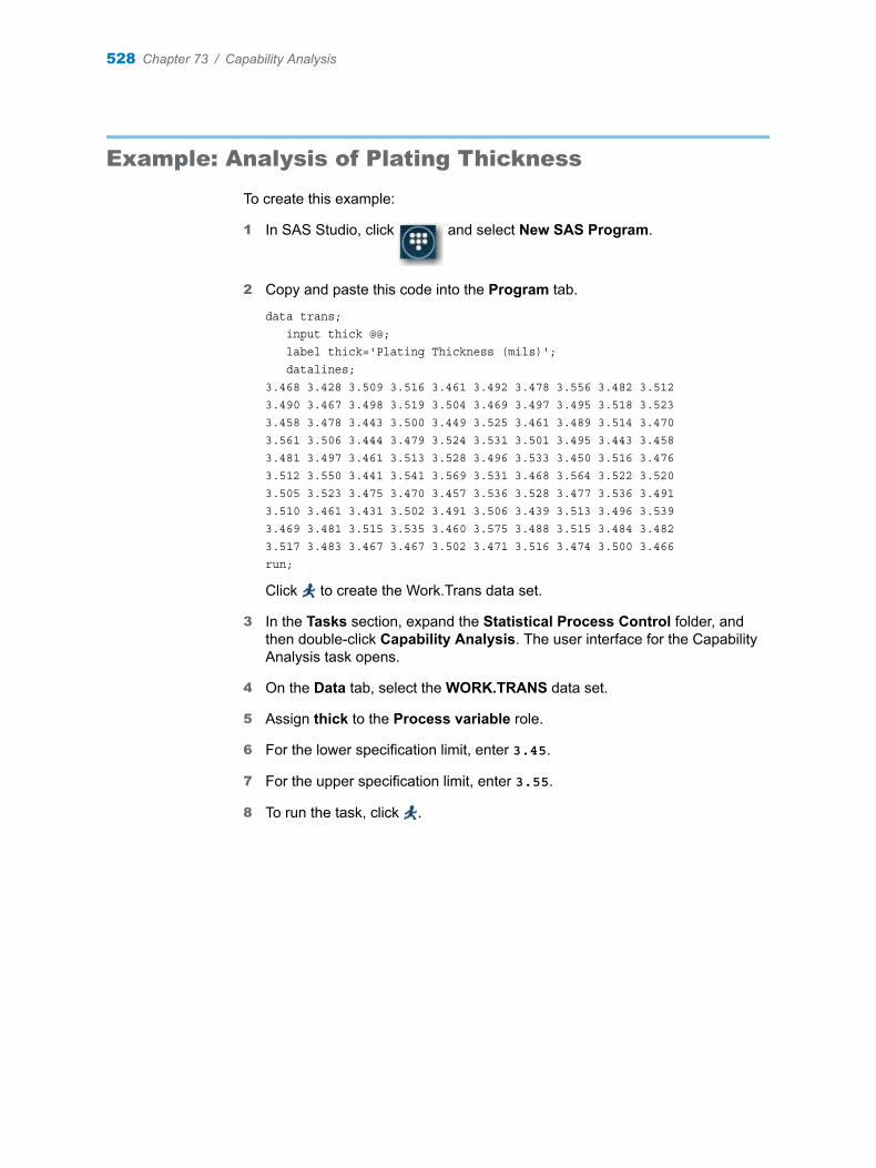
Example: Analysis of Plating Thickness
To create this example:
1 In SAS Studio, click and select New SAS Program.
2 Copy and paste this code into the Program tab.
data trans; input thick @@; label thick='Plating Thickness (mils)'; datalines;3.468 3.428 3.509 3.516 3.461 3.492 3.478 3.556 3.482 3.5123.490 3.467 3.498 3.519 3.504 3.469 3.497 3.495 3.518 3.5233.458 3.478 3.443 3.500 3.449 3.525 3.461 3.489 3.514 3.4703.561 3.506 3.444 3.479 3.524 3.531 3.501 3.495 3.443 3.4583.481 3.497 3.461 3.513 3.528 3.496 3.533 3.450 3.516 3.4763.512 3.550 3.441 3.541 3.569 3.531 3.468 3.564 3.522 3.5203.505 3.523 3.475 3.470 3.457 3.536 3.528 3.477 3.536 3.4913.510 3.461 3.431 3.502 3.491 3.506 3.439 3.513 3.496 3.5393.469 3.481 3.515 3.535 3.460 3.575 3.488 3.515 3.484 3.4823.517 3.483 3.467 3.467 3.502 3.471 3.516 3.474 3.500 3.466run;
Click to create the Work.Trans data set.
3 In the Tasks section, expand the Statistical Process Control folder, and then double-click Capability Analysis. The user interface for the Capability Analysis task opens.
4 On the Data tab, select the WORK.TRANS data set.
5 Assign thick to the Process variable role.
6 For the lower specification limit, enter 3.45.
7 For the upper specification limit, enter 3.55.
8 To run the task, click .
528 Chapter 73 / Capability Analysis

Here is a subset of the results:
Example: Analysis of Plating Thickness 529
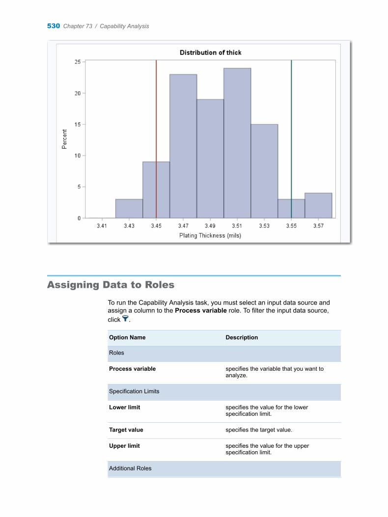
Assigning Data to Roles
To run the Capability Analysis task, you must select an input data source and assign a column to the Process variable role. To filter the input data source, click .
Option Name Description
Roles
Process variable specifies the variable that you want to analyze.
Specification Limits
Lower limit specifies the value for the lower specification limit.
Target value specifies the target value.
Upper limit specifies the value for the upper specification limit.
Additional Roles
530 Chapter 73 / Capability Analysis
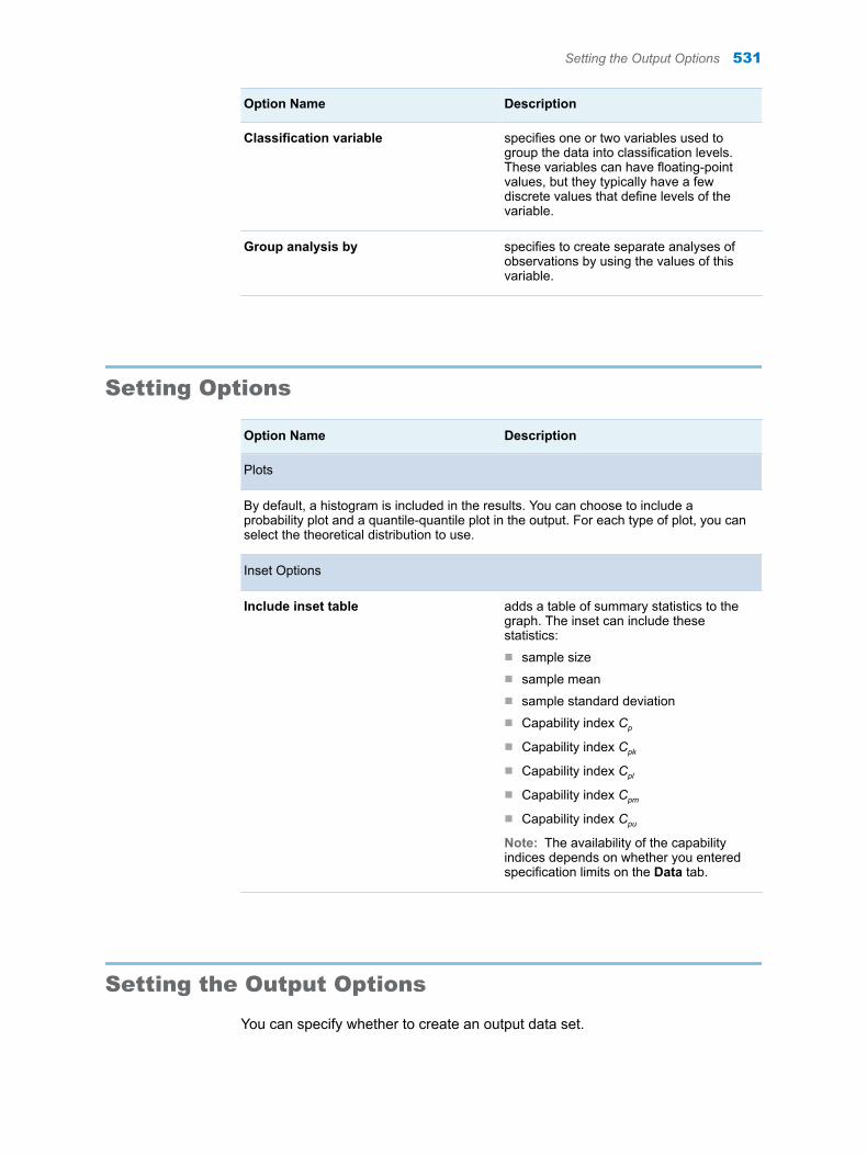
Option Name Description
Classification variable specifies one or two variables used to group the data into classification levels. These variables can have floating-point values, but they typically have a few discrete values that define levels of the variable.
Group analysis by specifies to create separate analyses of observations by using the values of this variable.
Setting Options
Option Name Description
Plots
By default, a histogram is included in the results. You can choose to include a probability plot and a quantile-quantile plot in the output. For each type of plot, you can select the theoretical distribution to use.
Inset Options
Include inset table adds a table of summary statistics to the graph. The inset can include these statistics:n sample sizen sample meann sample standard deviationn Capability index Cp
n Capability index Cpk
n Capability index Cpl
n Capability index Cpm
n Capability index Cpu
Note: The availability of the capability indices depends on whether you entered specification limits on the Data tab.
Setting the Output Options
You can specify whether to create an output data set.
Setting the Output Options 531

532 Chapter 73 / Capability Analysis
74Pareto Analysis
About the Pareto Analysis Task . . . . . . . . . . . . . . . . . . . . . . . . . . . . . . . . . . . . . . . . . . . 533
Example: Causes of Failure . . . . . . . . . . . . . . . . . . . . . . . . . . . . . . . . . . . . . . . . . . . . . . . . 533
Assigning Data to Roles . . . . . . . . . . . . . . . . . . . . . . . . . . . . . . . . . . . . . . . . . . . . . . . . . . . 535
Setting Options . . . . . . . . . . . . . . . . . . . . . . . . . . . . . . . . . . . . . . . . . . . . . . . . . . . . . . . . . . . . 536
Setting the Output Options . . . . . . . . . . . . . . . . . . . . . . . . . . . . . . . . . . . . . . . . . . . . . . . . 536
About the Pareto Analysis Task
Pareto charts display the frequencies of quality-related problems in a process. The frequencies are represented by bars that are ordered in decreasing magnitude. Thus, you can use a Pareto chart to decide which subset of problems to solve first or which problem areas deserve the most attention.
Example: Causes of Failure
During the manufacture of an MOS capacitor, different cleaning processes were used by two manufacturing systems operating in parallel. Process A used a standard cleaning solution, and Process B used a different cleaning mixture that contained less particulate matter. The failure causes that were observed with each process for five consecutive days were recorded. Now you want to compare the causes of the failure for each process.
To create this example:
1 In SAS Studio, click and select New SAS Program.
2 Copy and paste this code onto the Program tab.
data failure; length Cause $ 16; label Cause='Cause of Failure'; input Cause & $; datalines;CorrosionOxide Defect
533
ContaminationOxide DefectOxide DefectMiscellaneousOxide DefectContaminationMetallizationOxide DefectContaminationContaminationOxide DefectContaminationContaminationContaminationCorrosionSilicon DefectMiscellaneousContaminationContaminationContaminationMiscellaneousContaminationContaminationDopingOxide DefectOxide DefectMetallizationContaminationContaminationrun;
Click to create the Work.Failure data set.
3 In the Tasks section, expand the Statistical Process Control folder, and then double-click Pareto Analysis. The user interface for the Control Charts task opens.
4 On the Data tab, select the WORK.FAILURE data set.
TIP If the data set is not available from the drop-down list, click . In
the Choose a Table window, expand the library that contains the data set that you want to use. Select the data set for the example and click OK. The selected data set should now appear in the drop-down list.
5 To the Process variable role, assign the Cause variable.
6 To run the task, click .
534 Chapter 74 / Pareto Analysis
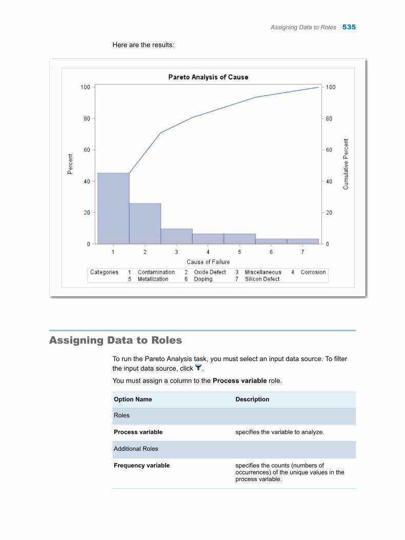
Here are the results:
Assigning Data to Roles
To run the Pareto Analysis task, you must select an input data source. To filter the input data source, click .
You must assign a column to the Process variable role.
Option Name Description
Roles
Process variable specifies the variable to analyze.
Additional Roles
Frequency variable specifies the counts (numbers of occurrences) of the unique values in the process variable.
Assigning Data to Roles 535

Option Name Description
Classification variable creates a comparative Pareto chart by using the levels of the variable.
Group analysis by enables you to obtain separate analyses of observations for each unique group.
Setting Options
Option Name Description
Plots
Select plot type uses either vertical or horizontal bars to measure the frequencies in the Pareto chart.
Display cumulative percentage curve displays the cumulative percentage curve.
Display sample size legend displays the legend for the sample size.
Number of categories to display requests that only the Pareto categories with the n highest frequencies be displayed.
Merge smaller categories merges smaller categories into one category to display on the Pareto chart.
Setting the Output Options
You can specify whether to create an output data set.
536 Chapter 74 / Pareto Analysis
75Analysis of Means
About the Analysis of Means Task . . . . . . . . . . . . . . . . . . . . . . . . . . . . . . . . . . . . . . . . . 537Mean Chart . . . . . . . . . . . . . . . . . . . . . . . . . . . . . . . . . . . . . . . . . . . . . . . . . . . . . . . . . . . . . 537Mean Chart with Boxes . . . . . . . . . . . . . . . . . . . . . . . . . . . . . . . . . . . . . . . . . . . . . . . . . . 538Proportion Chart . . . . . . . . . . . . . . . . . . . . . . . . . . . . . . . . . . . . . . . . . . . . . . . . . . . . . . . . 539Rate Chart . . . . . . . . . . . . . . . . . . . . . . . . . . . . . . . . . . . . . . . . . . . . . . . . . . . . . . . . . . . . . . 540
Example: Determine the Deviation of Label Positions . . . . . . . . . . . . . . . . . . . . . . 541
Assigning Data to Roles . . . . . . . . . . . . . . . . . . . . . . . . . . . . . . . . . . . . . . . . . . . . . . . . . . . 543
Setting Options . . . . . . . . . . . . . . . . . . . . . . . . . . . . . . . . . . . . . . . . . . . . . . . . . . . . . . . . . . . . 544
Setting the Output Options . . . . . . . . . . . . . . . . . . . . . . . . . . . . . . . . . . . . . . . . . . . . . . . . 545
About the Analysis of Means TaskAnalysis of means is a method for simultaneously comparing treatment means with their overall mean.
Mean Chart
The mean chart shows the deviation of the mean for the groups identified by the Group variable.
537
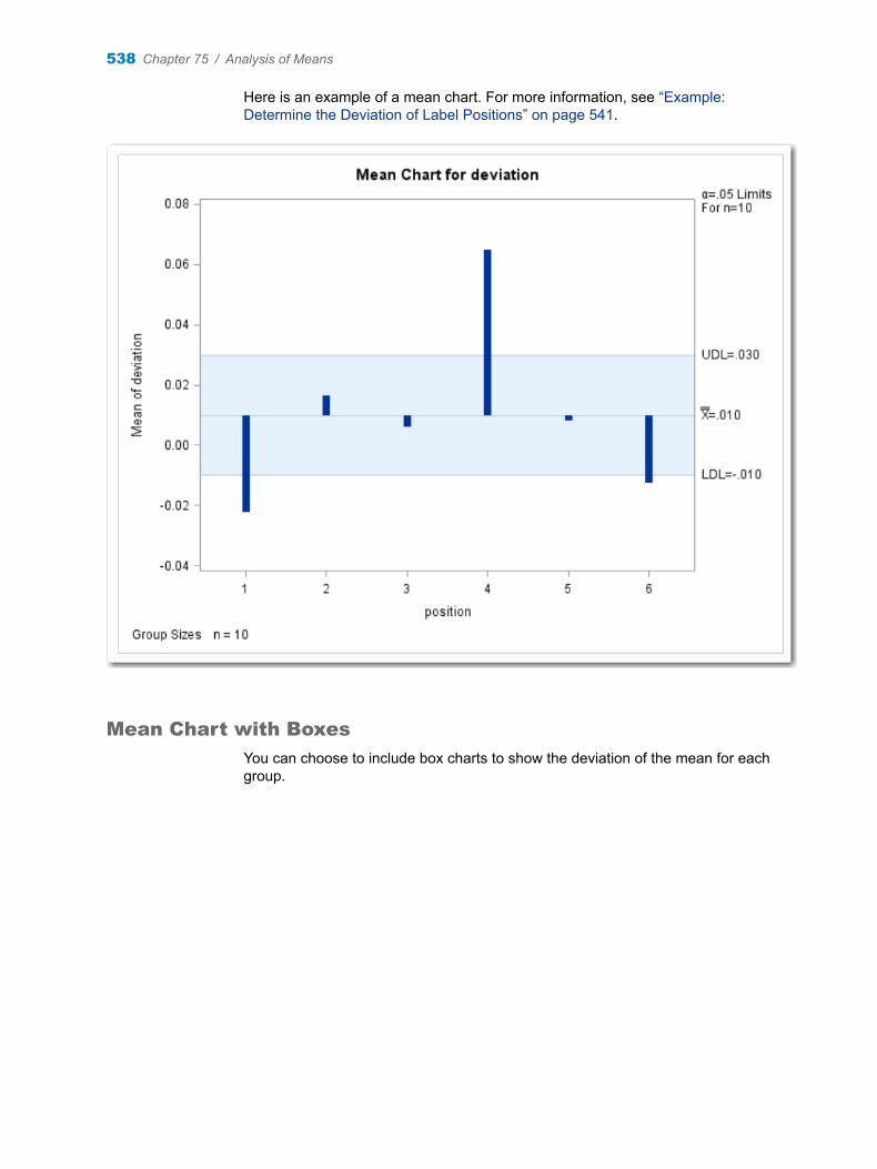
Here is an example of a mean chart. For more information, see “Example: Determine the Deviation of Label Positions” on page 541.
Mean Chart with Boxes
You can choose to include box charts to show the deviation of the mean for each group.
538 Chapter 75 / Analysis of Means
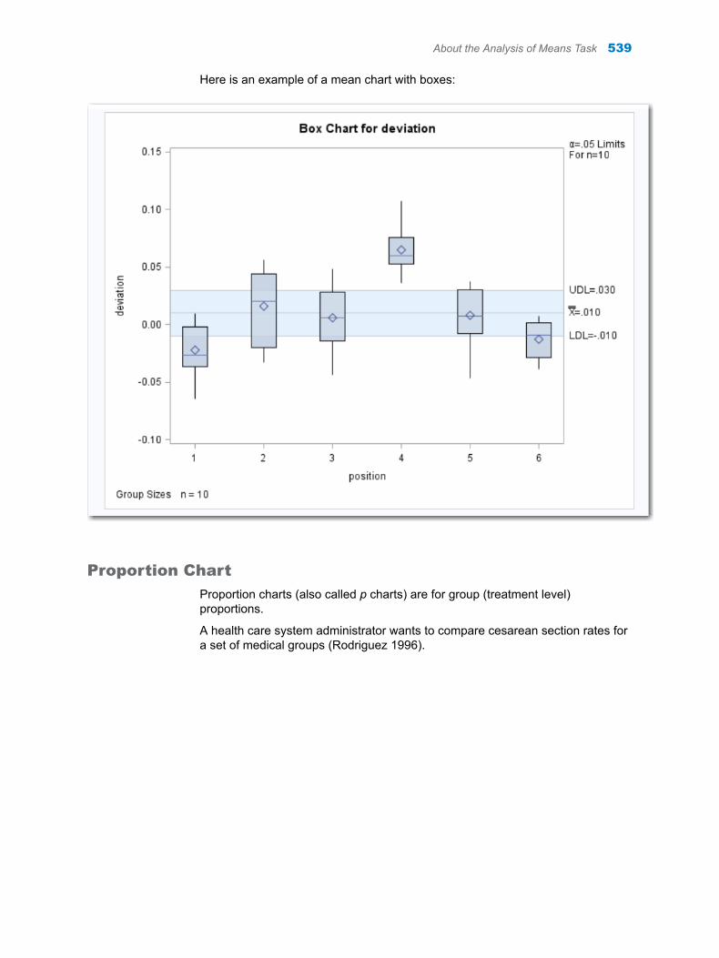
Here is an example of a mean chart with boxes:
Proportion Chart
Proportion charts (also called p charts) are for group (treatment level) proportions.
A health care system administrator wants to compare cesarean section rates for a set of medical groups (Rodriguez 1996).
About the Analysis of Means Task 539
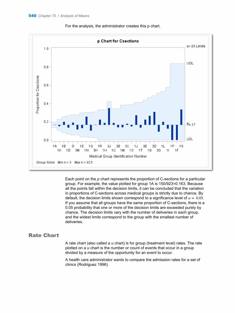
For the analysis, the administrator creates this p chart.
Each point on the p chart represents the proportion of C-sections for a particular group. For example, the value plotted for group 1A is 150/923=0.163. Because all the points fall within the decision limits, it can be concluded that the variation in proportions of C-sections across medical groups is strictly due to chance. By default, the decision limits shown correspond to a significance level of α = 0.05. If you assume that all groups have the same proportion of C-sections, there is a 0.05 probability that one or more of the decision limits are exceeded purely by chance. The decision limits vary with the number of deliveries in each group, and the widest limits correspond to the group with the smallest number of deliveries.
Rate Chart
A rate chart (also called a u chart) is for group (treatment level) rates. The rate plotted on a u chart is the number or count of events that occur in a group divided by a measure of the opportunity for an event to occur.
A health care administrator wants to compare the admission rates for a set of clinics (Rodriguez 1996).
540 Chapter 75 / Analysis of Means
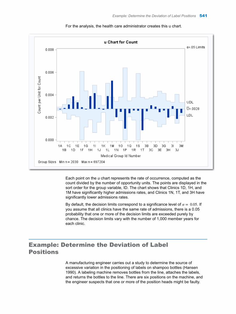
For the analysis, the health care administrator creates this u chart.
Each point on the u chart represents the rate of occurrence, computed as the count divided by the number of opportunity units. The points are displayed in the sort order for the group variable, ID. The chart shows that Clinics 1D, 1H, and 1M have significantly higher admissions rates, and Clinics 1N, 1T, and 3H have significantly lower admissions rates.
By default, the decision limits correspond to a significance level of α = 0.05. If you assume that all clinics have the same rate of admissions, there is a 0.05 probability that one or more of the decision limits are exceeded purely by chance. The decision limits vary with the number of 1,000 member years for each clinic.
Example: Determine the Deviation of Label Positions
A manufacturing engineer carries out a study to determine the source of excessive variation in the positioning of labels on shampoo bottles (Hansen 1990). A labeling machine removes bottles from the line, attaches the labels, and returns the bottles to the line. There are six positions on the machine, and the engineer suspects that one or more of the position heads might be faulty.
Example: Determine the Deviation of Label Positions 541
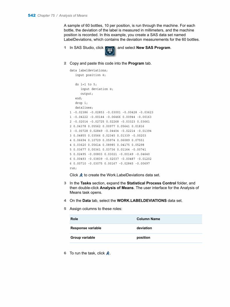
A sample of 60 bottles, 10 per position, is run through the machine. For each bottle, the deviation of the label is measured in millimeters, and the machine position is recorded. In this example, you create a SAS data set named LabelDeviations, which contains the deviation measurements for the 60 bottles.
1 In SAS Studio, click and select New SAS Program.
2 Copy and paste this code into the Program tab.
data labeldeviations; input position @; do i=1 to 5; input deviation @; output; end; drop i; datalines;1 -0.02386 -0.02853 -0.03001 -0.00428 -0.036231 -0.04222 -0.00144 -0.06466 0.00944 -0.001632 -0.02014 -0.02725 0.02268 -0.03323 0.036612 0.04378 0.05562 0.00977 0.05641 0.018163 -0.00728 0.02849 -0.04404 -0.02214 -0.013943 0.04855 0.03566 0.02345 0.01339 -0.002034 0.06694 0.10729 0.05974 0.06089 0.075514 0.03620 0.05614 0.08985 0.04175 0.052985 0.03677 0.00361 0.03736 0.01164 -0.007415 0.02495 -0.00803 0.03021 -0.00149 -0.046406 0.00493 -0.03839 -0.02037 -0.00487 -0.012026 0.00710 -0.03075 0.00167 -0.02845 -0.00697run;
Click to create the Work.LabelDeviations data set.
3 In the Tasks section, expand the Statistical Process Control folder, and then double-click Analysis of Means. The user interface for the Analysis of Means task opens.
4 On the Data tab, select the WORK.LABELDEVIATIONS data set.
5 Assign columns to these roles:
Role Column Name
Response variable deviation
Group variable position
6 To run the task, click .
542 Chapter 75 / Analysis of Means

Here are the results:
Each point on the chart represents the average (mean) of the response measurements for a particular sample. The average for Position 1 is below the lower decision limit (LDL), and the average for Position 6 is slightly below the lower decision limit. The average for Position 4 exceeds the upper decision limit (UDL). The conclusion is that Positions 1, 4, and 6 are operating differently.
Assigning Data to Roles
To run the Analysis of Means task, you must select an input data source and assign a column to the Response variable and Group variable roles. To filter the input data source, click .
Option Name Description
Roles
Response variable specifies the responses to analyze.
Assigning Data to Roles 543
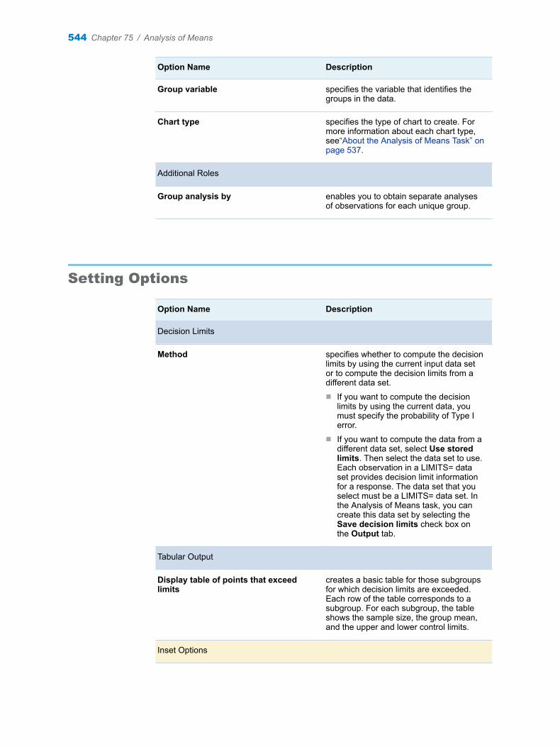
Option Name Description
Group variable specifies the variable that identifies the groups in the data.
Chart type specifies the type of chart to create. For more information about each chart type, see“About the Analysis of Means Task” on page 537.
Additional Roles
Group analysis by enables you to obtain separate analyses of observations for each unique group.
Setting Options
Option Name Description
Decision Limits
Method specifies whether to compute the decision limits by using the current input data set or to compute the decision limits from a different data set.n If you want to compute the decision
limits by using the current data, you must specify the probability of Type I error.
n If you want to compute the data from a different data set, select Use stored limits. Then select the data set to use. Each observation in a LIMITS= data set provides decision limit information for a response. The data set that you select must be a LIMITS= data set. In the Analysis of Means task, you can create this data set by selecting the Save decision limits check box on the Output tab.
Tabular Output
Display table of points that exceed limits
creates a basic table for those subgroups for which decision limits are exceeded. Each row of the table corresponds to a subgroup. For each subgroup, the table shows the sample size, the group mean, and the upper and lower control limits.
Inset Options
544 Chapter 75 / Analysis of Means
Option Name Description
You can specify whether to include an insert table in the output. You can also choose the statistics to include in this table: significance level, degrees of freedom, average of group means, and mean square error.
Setting the Output Options
You can choose to create a decision limits data set or a data set that contains both the statistics and decision limits.
Setting the Output Options 545

546 Chapter 75 / Analysis of Means

Part 11
Data Mining Tasks
Chapter 76Rapid Predictive Modeler . . . . . . . . . . . . . . . . . . . . . . . . . . . . . . . . . . . . . . . . . 549
547

548
76Rapid Predictive Modeler
About the Rapid Predictive Modeler . . . . . . . . . . . . . . . . . . . . . . . . . . . . . . . . . . . . . . . 549Overview of the Rapid Predictive Modeler . . . . . . . . . . . . . . . . . . . . . . . . . . . . . . . . . 549Sampling Strategies for the SAS Rapid Predictive Modeler . . . . . . . . . . . . . . . . . 550Organizing Data for the SAS Rapid Predictive Modeler . . . . . . . . . . . . . . . . . . . . . 551Reserved Prefixes for Variables . . . . . . . . . . . . . . . . . . . . . . . . . . . . . . . . . . . . . . . . . . 552
Assigning Data to Roles . . . . . . . . . . . . . . . . . . . . . . . . . . . . . . . . . . . . . . . . . . . . . . . . . . . 553
Setting the Model Options . . . . . . . . . . . . . . . . . . . . . . . . . . . . . . . . . . . . . . . . . . . . . . . . . 555Choosing a Model . . . . . . . . . . . . . . . . . . . . . . . . . . . . . . . . . . . . . . . . . . . . . . . . . . . . . . . 555Modeling Methods . . . . . . . . . . . . . . . . . . . . . . . . . . . . . . . . . . . . . . . . . . . . . . . . . . . . . . . 555Understanding the Models for the SAS Rapid Predictive Modeler . . . . . . . . . . . 556
Setting the Report Options . . . . . . . . . . . . . . . . . . . . . . . . . . . . . . . . . . . . . . . . . . . . . . . . 558About the Reports . . . . . . . . . . . . . . . . . . . . . . . . . . . . . . . . . . . . . . . . . . . . . . . . . . . . . . . 558About the Standard Reports for the SAS Rapid Predictive Modeler . . . . . . . . . . 559
Setting the Output Options . . . . . . . . . . . . . . . . . . . . . . . . . . . . . . . . . . . . . . . . . . . . . . . . 559
About the Rapid Predictive Modeler
Overview of the Rapid Predictive Modeler
SAS Rapid Predictive Modeler is designed to build models for the following types of data mining classification and regression problems:
n classification models that predict the value of a discrete variable. Some examples are classification models that predict the value of a variable, such as True or False; Purchase or Decline; High, Medium, or Low; and Churn or Continues.
n regression models that predict the value of a continuous variable. Some examples are regression models that might predict amounts such as revenue, sales, or success rate by using continuous values.
To create a model by using the SAS Rapid Predictive Modeler, you must supply a data set, where every row contains a set of independent predictor variables (known as inputs) and at least one dependent variable (known as a target). The SAS Rapid Predictive Modeler decides whether variables are continuous or categorical, and chooses the input variables that should be included in the model.
549
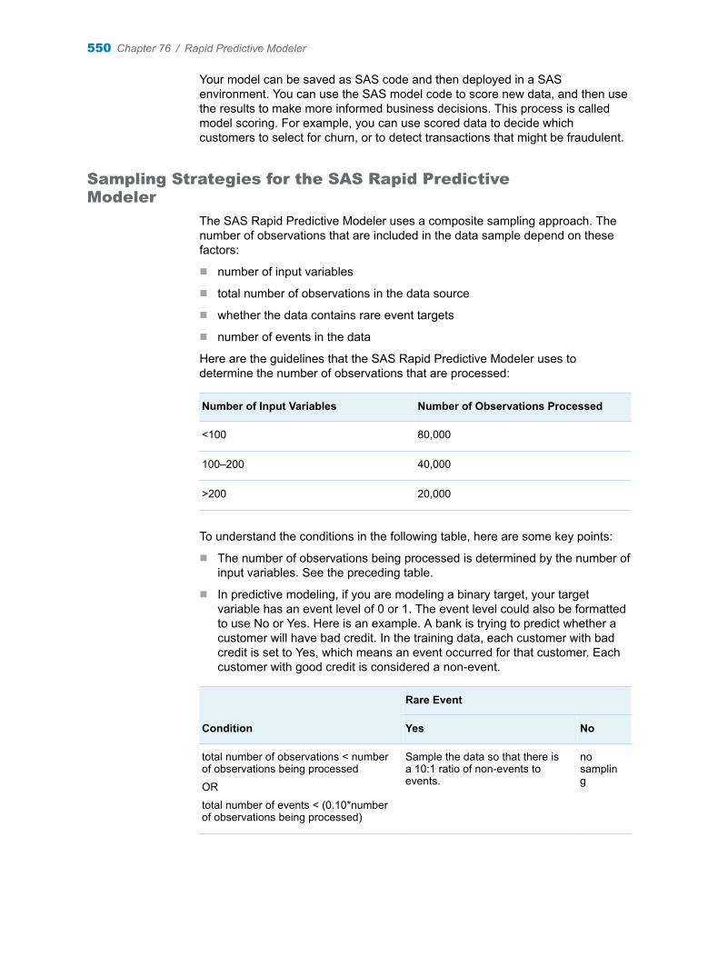
Your model can be saved as SAS code and then deployed in a SAS environment. You can use the SAS model code to score new data, and then use the results to make more informed business decisions. This process is called model scoring. For example, you can use scored data to decide which customers to select for churn, or to detect transactions that might be fraudulent.
Sampling Strategies for the SAS Rapid Predictive Modeler
The SAS Rapid Predictive Modeler uses a composite sampling approach. The number of observations that are included in the data sample depend on these factors:
n number of input variables
n total number of observations in the data source
n whether the data contains rare event targets
n number of events in the data
Here are the guidelines that the SAS Rapid Predictive Modeler uses to determine the number of observations that are processed:
Number of Input Variables Number of Observations Processed
<100 80,000
100–200 40,000
>200 20,000
To understand the conditions in the following table, here are some key points:
n The number of observations being processed is determined by the number of input variables. See the preceding table.
n In predictive modeling, if you are modeling a binary target, your target variable has an event level of 0 or 1. The event level could also be formatted to use No or Yes. Here is an example. A bank is trying to predict whether a customer will have bad credit. In the training data, each customer with bad credit is set to Yes, which means an event occurred for that customer. Each customer with good credit is considered a non-event.
Condition
Rare Event
Yes No
total number of observations < number of observations being processed
OR
total number of events < (0.10*number of observations being processed)
Sample the data so that there is a 10:1 ratio of non-events to events.
no sampling
550 Chapter 76 / Rapid Predictive Modeler
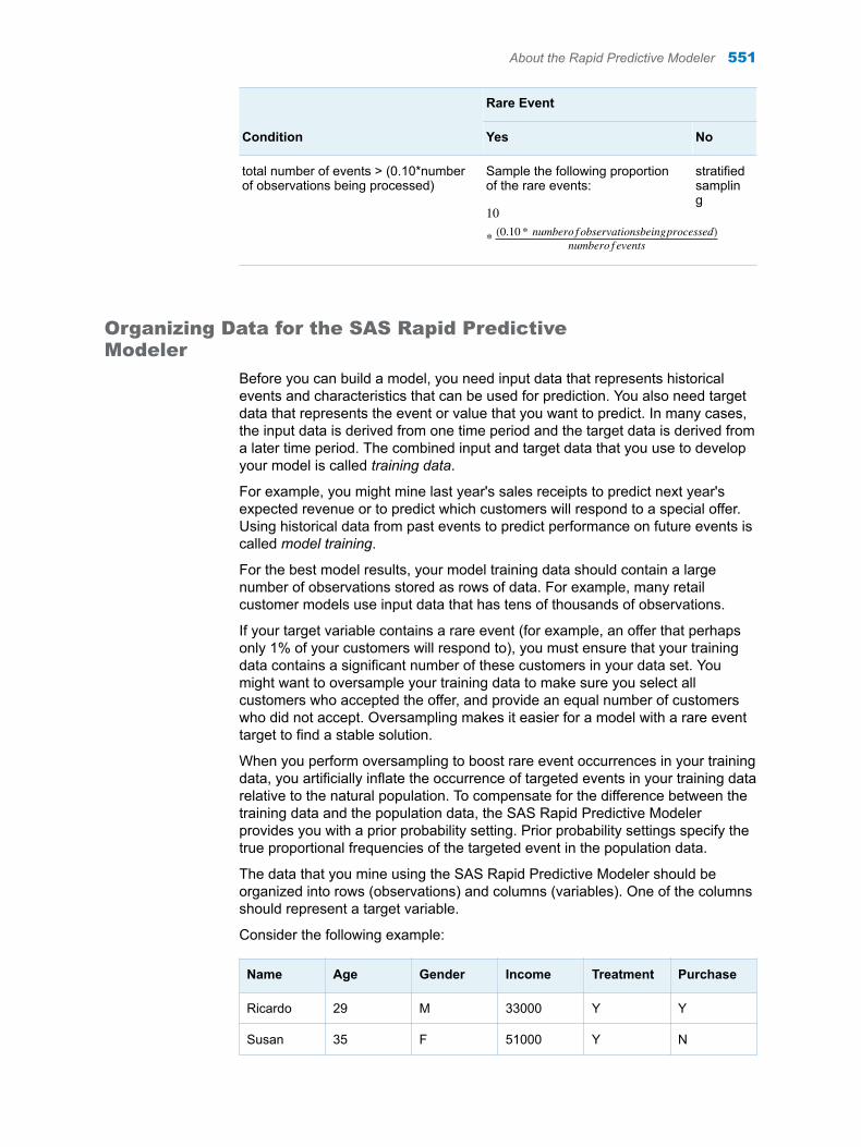
Condition
Rare Event
Yes No
total number of events > (0.10*number of observations being processed)
Sample the following proportion of the rare events:
10
* 0.10 * numbero f observationsbeingprocessednumbero f events
stratified sampling
Organizing Data for the SAS Rapid Predictive Modeler
Before you can build a model, you need input data that represents historical events and characteristics that can be used for prediction. You also need target data that represents the event or value that you want to predict. In many cases, the input data is derived from one time period and the target data is derived from a later time period. The combined input and target data that you use to develop your model is called training data.
For example, you might mine last year's sales receipts to predict next year's expected revenue or to predict which customers will respond to a special offer. Using historical data from past events to predict performance on future events is called model training.
For the best model results, your model training data should contain a large number of observations stored as rows of data. For example, many retail customer models use input data that has tens of thousands of observations.
If your target variable contains a rare event (for example, an offer that perhaps only 1% of your customers will respond to), you must ensure that your training data contains a significant number of these customers in your data set. You might want to oversample your training data to make sure you select all customers who accepted the offer, and provide an equal number of customers who did not accept. Oversampling makes it easier for a model with a rare event target to find a stable solution.
When you perform oversampling to boost rare event occurrences in your training data, you artificially inflate the occurrence of targeted events in your training data relative to the natural population. To compensate for the difference between the training data and the population data, the SAS Rapid Predictive Modeler provides you with a prior probability setting. Prior probability settings specify the true proportional frequencies of the targeted event in the population data.
The data that you mine using the SAS Rapid Predictive Modeler should be organized into rows (observations) and columns (variables). One of the columns should represent a target variable.
Consider the following example:
Name Age Gender Income Treatment Purchase
Ricardo 29 M 33000 Y Y
Susan 35 F 51000 Y N
About the Rapid Predictive Modeler 551
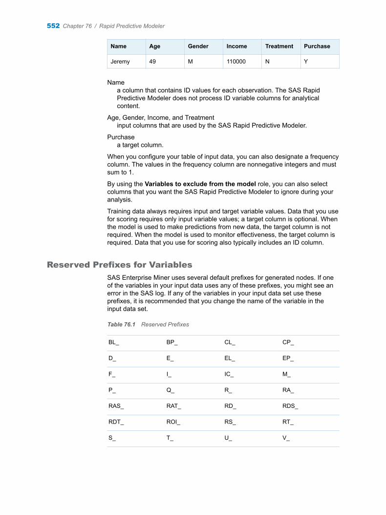
Name Age Gender Income Treatment Purchase
Jeremy 49 M 110000 N Y
Namea column that contains ID values for each observation. The SAS Rapid Predictive Modeler does not process ID variable columns for analytical content.
Age, Gender, Income, and Treatmentinput columns that are used by the SAS Rapid Predictive Modeler.
Purchasea target column.
When you configure your table of input data, you can also designate a frequency column. The values in the frequency column are nonnegative integers and must sum to 1.
By using the Variables to exclude from the model role, you can also select columns that you want the SAS Rapid Predictive Modeler to ignore during your analysis.
Training data always requires input and target variable values. Data that you use for scoring requires only input variable values; a target column is optional. When the model is used to make predictions from new data, the target column is not required. When the model is used to monitor effectiveness, the target column is required. Data that you use for scoring also typically includes an ID column.
Reserved Prefixes for Variables
SAS Enterprise Miner uses several default prefixes for generated nodes. If one of the variables in your input data uses any of these prefixes, you might see an error in the SAS log. If any of the variables in your input data set use these prefixes, it is recommended that you change the name of the variable in the input data set.
Table 76.1 Reserved Prefixes
BL_ BP_ CL_ CP_
D_ E_ EL_ EP_
F_ I_ IC_ M_
P_ Q_ R_ RA_
RAS_ RAT_ RD_ RDS_
RDT_ ROI_ RS_ RT_
S_ T_ U_ V_
552 Chapter 76 / Rapid Predictive Modeler
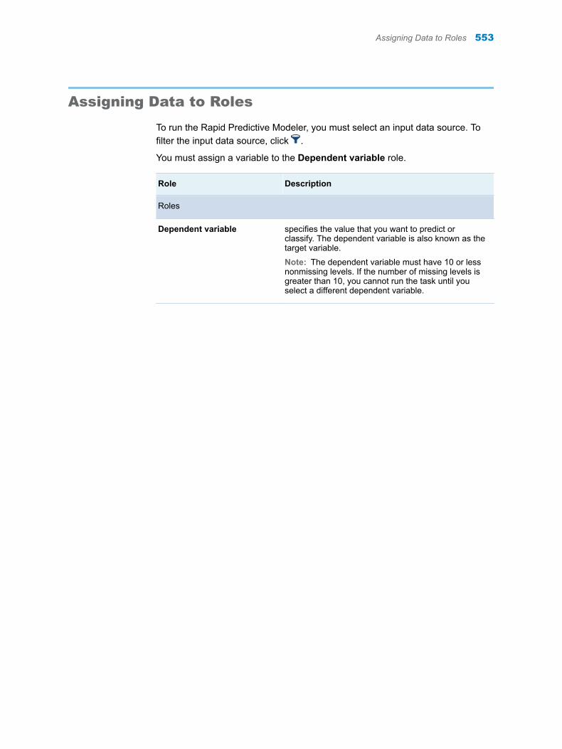
Assigning Data to Roles
To run the Rapid Predictive Modeler, you must select an input data source. To filter the input data source, click .
You must assign a variable to the Dependent variable role.
Role Description
Roles
Dependent variable specifies the value that you want to predict or classify. The dependent variable is also known as the target variable.
Note: The dependent variable must have 10 or less nonmissing levels. If the number of missing levels is greater than 10, you cannot run the task until you select a different dependent variable.
Assigning Data to Roles 553
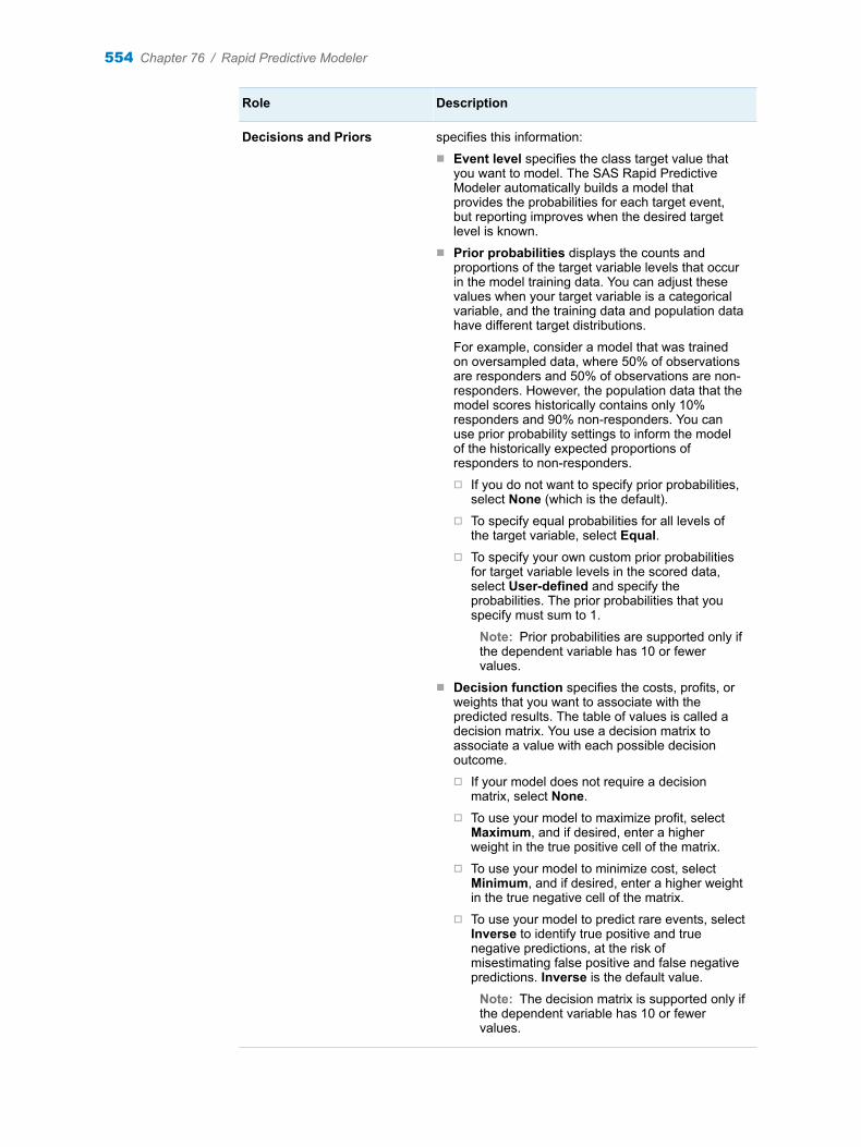
Role Description
Decisions and Priors specifies this information:n Event level specifies the class target value that
you want to model. The SAS Rapid Predictive Modeler automatically builds a model that provides the probabilities for each target event, but reporting improves when the desired target level is known.
n Prior probabilities displays the counts and proportions of the target variable levels that occur in the model training data. You can adjust these values when your target variable is a categorical variable, and the training data and population data have different target distributions.
For example, consider a model that was trained on oversampled data, where 50% of observations are responders and 50% of observations are non-responders. However, the population data that the model scores historically contains only 10% responders and 90% non-responders. You can use prior probability settings to inform the model of the historically expected proportions of responders to non-responders.o If you do not want to specify prior probabilities,
select None (which is the default). o To specify equal probabilities for all levels of
the target variable, select Equal. o To specify your own custom prior probabilities
for target variable levels in the scored data, select User-defined and specify the probabilities. The prior probabilities that you specify must sum to 1.
Note: Prior probabilities are supported only if the dependent variable has 10 or fewer values.
n Decision function specifies the costs, profits, or weights that you want to associate with the predicted results. The table of values is called a decision matrix. You use a decision matrix to associate a value with each possible decision outcome. o If your model does not require a decision
matrix, select None.o To use your model to maximize profit, select
Maximum, and if desired, enter a higher weight in the true positive cell of the matrix.
o To use your model to minimize cost, select Minimum, and if desired, enter a higher weight in the true negative cell of the matrix.
o To use your model to predict rare events, select Inverse to identify true positive and true negative predictions, at the risk of misestimating false positive and false negative predictions. Inverse is the default value.
Note: The decision matrix is supported only if the dependent variable has 10 or fewer values.
554 Chapter 76 / Rapid Predictive Modeler
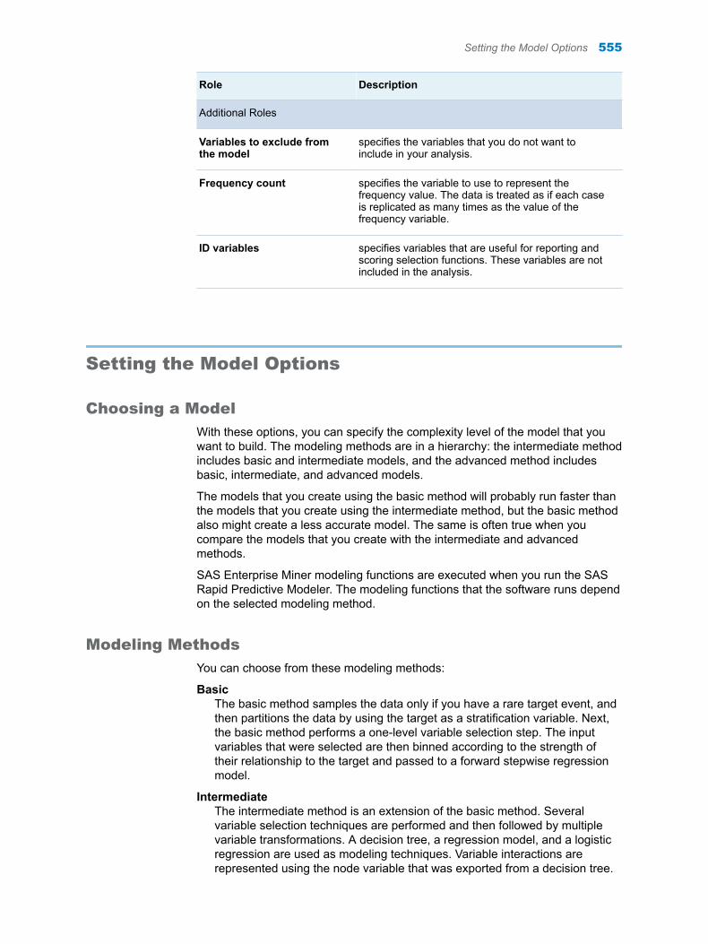
Role Description
Additional Roles
Variables to exclude from the model
specifies the variables that you do not want to include in your analysis.
Frequency count specifies the variable to use to represent the frequency value. The data is treated as if each case is replicated as many times as the value of the frequency variable.
ID variables specifies variables that are useful for reporting and scoring selection functions. These variables are not included in the analysis.
Setting the Model Options
Choosing a Model
With these options, you can specify the complexity level of the model that you want to build. The modeling methods are in a hierarchy: the intermediate method includes basic and intermediate models, and the advanced method includes basic, intermediate, and advanced models.
The models that you create using the basic method will probably run faster than the models that you create using the intermediate method, but the basic method also might create a less accurate model. The same is often true when you compare the models that you create with the intermediate and advanced methods.
SAS Enterprise Miner modeling functions are executed when you run the SAS Rapid Predictive Modeler. The modeling functions that the software runs depend on the selected modeling method.
Modeling Methods
You can choose from these modeling methods:
BasicThe basic method samples the data only if you have a rare target event, and then partitions the data by using the target as a stratification variable. Next, the basic method performs a one-level variable selection step. The input variables that were selected are then binned according to the strength of their relationship to the target and passed to a forward stepwise regression model.
IntermediateThe intermediate method is an extension of the basic method. Several variable selection techniques are performed and then followed by multiple variable transformations. A decision tree, a regression model, and a logistic regression are used as modeling techniques. Variable interactions are represented using the node variable that was exported from a decision tree.
Setting the Model Options 555

The intermediate method also runs the basic method, and then chooses the best performing model.
AdvancedThe advanced method is an extension of the intermediate method and includes a neural network model, an advanced regression analysis, and ensemble models. The advanced method also runs the intermediate and basic methods, and then chooses the best performing model.
Understanding the Models for the SAS Rapid Predictive Modeler
The SAS Rapid Predictive Modeler provides you with basic, intermediate, and advanced models. The models increase in sophistication and complexity.
n The basic model is a simple regression analysis.
n The intermediate model includes a more sophisticated analysis, plus the analysis from the basic model, and chooses the better model.
n The advanced model includes an even more sophisticated analysis, plus the analyses from the basic and intermediate models, and chooses the best model.
BasicThe basic model performs a series of three data mining operations.
n Variable Selection: The basic model chooses the top 100 variables for modeling.
n Transformation: The basic model performs an Optimal Binning transformation on the top 100 variables selected for modeling. The Optimal Binning transformation compensates for missing variable values, so missing value imputation is not performed.
n Modeling: The basic model uses a forward regression model. The forward regression model chooses variables one at a time in a stepwise process. The stepwise process adds one variable at a time to the linear equation until the variable contributions are insignificant. The forward regression model seeks to exclude variables with no predictive ability (or variables that are highly correlated with other predictor variables) from the analytic analysis.
IntermediateThe intermediate model performs a series of seven data mining operations.
n Variable Selection: The intermediate model chooses the top 200 variables for modeling.
n Transformation: The intermediate model performs a best power transformation on the 200 variables that were selected for modeling. The best power transformations are a subset of the general class of transformations that are known as Box-Cox transformations. The best power transformation evaluates a subset of exponential power transformations, and then chooses the transformation that has the best results for the specified criterion.
n Imputation: The intermediate model performs an imputation to replace missing variables with the average variable values. The imputation operation also creates indicator variables that enable observations that contain imputed variable values to be identified.
556 Chapter 76 / Rapid Predictive Modeler
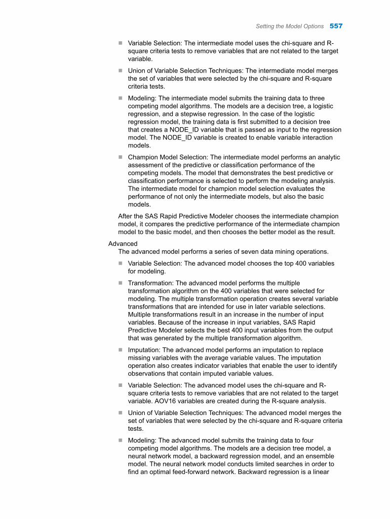
n Variable Selection: The intermediate model uses the chi-square and R-square criteria tests to remove variables that are not related to the target variable.
n Union of Variable Selection Techniques: The intermediate model merges the set of variables that were selected by the chi-square and R-square criteria tests.
n Modeling: The intermediate model submits the training data to three competing model algorithms. The models are a decision tree, a logistic regression, and a stepwise regression. In the case of the logistic regression model, the training data is first submitted to a decision tree that creates a NODE_ID variable that is passed as input to the regression model. The NODE_ID variable is created to enable variable interaction models.
n Champion Model Selection: The intermediate model performs an analytic assessment of the predictive or classification performance of the competing models. The model that demonstrates the best predictive or classification performance is selected to perform the modeling analysis. The intermediate model for champion model selection evaluates the performance of not only the intermediate models, but also the basic models.
After the SAS Rapid Predictive Modeler chooses the intermediate champion model, it compares the predictive performance of the intermediate champion model to the basic model, and then chooses the better model as the result.
AdvancedThe advanced model performs a series of seven data mining operations.
n Variable Selection: The advanced model chooses the top 400 variables for modeling.
n Transformation: The advanced model performs the multiple transformation algorithm on the 400 variables that were selected for modeling. The multiple transformation operation creates several variable transformations that are intended for use in later variable selections. Multiple transformations result in an increase in the number of input variables. Because of the increase in input variables, SAS Rapid Predictive Modeler selects the best 400 input variables from the output that was generated by the multiple transformation algorithm.
n Imputation: The advanced model performs an imputation to replace missing variables with the average variable values. The imputation operation also creates indicator variables that enable the user to identify observations that contain imputed variable values.
n Variable Selection: The advanced model uses the chi-square and R-square criteria tests to remove variables that are not related to the target variable. AOV16 variables are created during the R-square analysis.
n Union of Variable Selection Techniques: The advanced model merges the set of variables that were selected by the chi-square and R-square criteria tests.
n Modeling: The advanced model submits the training data to four competing model algorithms. The models are a decision tree model, a neural network model, a backward regression model, and an ensemble model. The neural network model conducts limited searches in order to find an optimal feed-forward network. Backward regression is a linear
Setting the Model Options 557
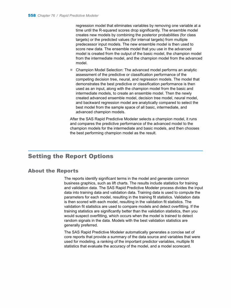
regression model that eliminates variables by removing one variable at a time until the R-squared scores drop significantly. The ensemble model creates new models by combining the posterior probabilities (for class targets) or the predicted values (for interval targets) from multiple predecessor input models. The new ensemble model is then used to score new data. The ensemble model that you use in the advanced model is created from the output of the basic model, the champion model from the intermediate model, and the champion model from the advanced model.
n Champion Model Selection: The advanced model performs an analytic assessment of the predictive or classification performance of the competing decision tree, neural, and regression models. The model that demonstrates the best predictive or classification performance is then used as an input, along with the champion model from the basic and intermediate models, to create an ensemble model. Then the newly created advanced ensemble model, decision tree model, neural model, and backward regression model are analytically compared to select the best model from the sample space of all basic, intermediate, and advanced champion models.
After the SAS Rapid Predictive Modeler selects a champion model, it runs and compares the predictive performance of the advanced model to the champion models for the intermediate and basic models, and then chooses the best performing champion model as the result.
Setting the Report Options
About the Reports
The reports identify significant terms in the model and generate common business graphics, such as lift charts. The results include statistics for training and validation data. The SAS Rapid Predictive Modeler process divides the input data into training data and validation data. Training data is used to compute the parameters for each model, resulting in the training fit statistics. Validation data is then scored with each model, resulting in the validation fit statistics. The validation fit statistics are used to compare models and detect overfitting. If the training statistics are significantly better than the validation statistics, then you would suspect overfitting, which occurs when the model is trained to detect random signals in the data. Models with the best validation statistics are generally preferred.
The SAS Rapid Predictive Modeler automatically generates a concise set of core reports that provide a summary of the data source and variables that were used for modeling, a ranking of the important predictor variables, multiple fit statistics that evaluate the accuracy of the model, and a model scorecard.
558 Chapter 76 / Rapid Predictive Modeler
About the Standard Reports for the SAS Rapid Predictive Modeler
Here are the standard reports that are automatically generated by the SAS Rapid Predictive Modeler:
Gains chartGains chart plots are available only for models that have class target variables. This chart shows percentiles of the data ranked by predicted value. Lift is a measure of the ratio of the number of target events that the model identified, compared to the number of target events that were found by random selection.
Receiver Operating Characteristic plot (ROC)The Receiver Operating Characteristic plot shows the maximum predictive power of a model for the entire sample (rather than for a single decile). The data is plotted as sensitivity versus (1 – specificity). The separation between the model curve and the diagonal line (which represents a random selection model) is called the Kolmogorov-Smirnov (KS) value. Higher KS values represent more powerful models.
ScorecardThe results include a scorecard so that the model's characteristics can be interpreted for business purposes. When the software builds a scorecard, each interval variable is binned into distinct ranges of values. Then, each variable is ranked by model importance and scaled to a maximum of 1,000 points. The distinct value for each variable then receives a portion of the scaled point total.
Project informationThe project information shows which user created the model, when the model was created, and where the model's component files are stored.
Setting the Output Options
Option Description
Output Data Set
Setting the Output Options 559

Option Description
Save Enterprise Miner project data
specifies whether to save the SAS Enterprise Miner data from this task. A model from the SAS Rapid Predictive Modeler is an example of a SAS Enterprise Miner project. When you save SAS Enterprise Miner data, you can use the SAS Enterprise Miner interface to open and edit the model that you created using the SAS Rapid Predictive Modeler. In SAS Enterprise Miner, you can save and export your analysis for use outside of SAS Enterprise Miner, and register your model with a SAS Metadata Repository.n If you have a workstation installation of SAS Enterprise
Miner, the project is saved locally in the workstation location that is specified.
n If you have a client/server installation of SAS Enterprise Miner, the project is saved in the User Root folder (for example, C:\users\username\Documents) on the server. If you used SAS Management Console to define a SYSTEM root location (for example, C:\projects) on the server, no directory path is specified. In this case, you can specify the location for your project storage. If this field is left blank and you do not specify a location before attempting to save the project, an error message is displayed that prompts you to specify a valid location.
The project data for several runs of the Rapid Predictive Modeler task can be saved in the same folder.
Export scoring code
saves the scoring code from this task to the specified location. You can then run this code to score other sets of data in other SAS products.
Score input data set specifies the name of the output data set that contains the scored values. The values in the input data set are scored by the model that the SAS Rapid Predictive Modeler builds.
560 Chapter 76 / Rapid Predictive Modeler
Part 12
Appendixes
Appendix 1Input Data Sets for Task Examples . . . . . . . . . . . . . . . . . . . . . . . . . . . . . . . . 563
Appendix 2References . . . . . . . . . . . . . . . . . . . . . . . . . . . . . . . . . . . . . . . . . . . . . . . . . . . . . 623
561

562

Appendix 1Input Data Sets for Task Examples
About the Task Data Sets . . . . . . . . . . . . . . . . . . . . . . . . . . . . . . . . . . . . . . . . . . . . . . . . . . 563
CIGAR Data Set . . . . . . . . . . . . . . . . . . . . . . . . . . . . . . . . . . . . . . . . . . . . . . . . . . . . . . . . . . . 563
FITNESS Data set . . . . . . . . . . . . . . . . . . . . . . . . . . . . . . . . . . . . . . . . . . . . . . . . . . . . . . . . . . 588
GETSTARTED Data Set . . . . . . . . . . . . . . . . . . . . . . . . . . . . . . . . . . . . . . . . . . . . . . . . . . . . 589
GREENE Data Set . . . . . . . . . . . . . . . . . . . . . . . . . . . . . . . . . . . . . . . . . . . . . . . . . . . . . . . . . 591
IN Data Set . . . . . . . . . . . . . . . . . . . . . . . . . . . . . . . . . . . . . . . . . . . . . . . . . . . . . . . . . . . . . . . . 591
LONG97DATA Data Set . . . . . . . . . . . . . . . . . . . . . . . . . . . . . . . . . . . . . . . . . . . . . . . . . . . . 592
MROZ Data Set . . . . . . . . . . . . . . . . . . . . . . . . . . . . . . . . . . . . . . . . . . . . . . . . . . . . . . . . . . . . 608
About the Task Data Sets
To complete some of the examples in the task documentation, you might need to create one or more data sets. This appendix provides the SAS code that you need. To create these data sets, copy and paste this code (from the HTML version of SAS Studio: User's Guide) into a Program tab in SAS Studio and click .
CIGAR Data Set
To create the Cigar data set, enter this code into a Program tab:
data cigar; input state year price pop pop_16 cpi ndi sales pimin; label state = 'State abbreviation' year = 'YEAR' price = 'Price per pack of cigarettes' pop = 'Population' pop_16 = 'Population above the age of 16' cpi = 'Consumer price index with (1983=100)' ndi = 'Per capita disposable income' sales = 'Cigarette sales in packs per capita' pimin = 'Minimum price in adjoining states per pack of cigarettes';
563
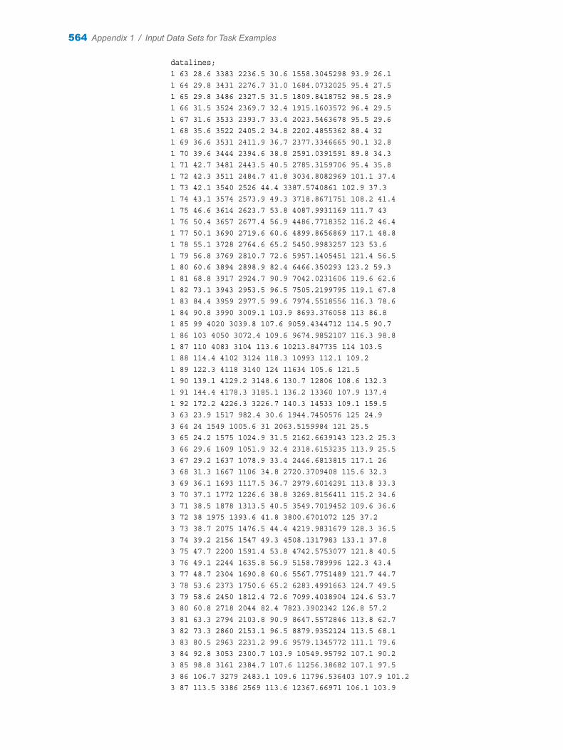
datalines; 1 63 28.6 3383 2236.5 30.6 1558.3045298 93.9 26.1 1 64 29.8 3431 2276.7 31.0 1684.0732025 95.4 27.5 1 65 29.8 3486 2327.5 31.5 1809.8418752 98.5 28.9 1 66 31.5 3524 2369.7 32.4 1915.1603572 96.4 29.5 1 67 31.6 3533 2393.7 33.4 2023.5463678 95.5 29.6 1 68 35.6 3522 2405.2 34.8 2202.4855362 88.4 32 1 69 36.6 3531 2411.9 36.7 2377.3346665 90.1 32.8 1 70 39.6 3444 2394.6 38.8 2591.0391591 89.8 34.3 1 71 42.7 3481 2443.5 40.5 2785.3159706 95.4 35.8 1 72 42.3 3511 2484.7 41.8 3034.8082969 101.1 37.4 1 73 42.1 3540 2526 44.4 3387.5740861 102.9 37.3 1 74 43.1 3574 2573.9 49.3 3718.8671751 108.2 41.4 1 75 46.6 3614 2623.7 53.8 4087.9931169 111.7 43 1 76 50.4 3657 2677.4 56.9 4486.7718352 116.2 46.4 1 77 50.1 3690 2719.6 60.6 4899.8656869 117.1 48.8 1 78 55.1 3728 2764.6 65.2 5450.9983257 123 53.6 1 79 56.8 3769 2810.7 72.6 5957.1405451 121.4 56.5 1 80 60.6 3894 2898.9 82.4 6466.350293 123.2 59.3 1 81 68.8 3917 2924.7 90.9 7042.0231606 119.6 62.6 1 82 73.1 3943 2953.5 96.5 7505.2199795 119.1 67.8 1 83 84.4 3959 2977.5 99.6 7974.5518556 116.3 78.6 1 84 90.8 3990 3009.1 103.9 8693.376058 113 86.8 1 85 99 4020 3039.8 107.6 9059.4344712 114.5 90.7 1 86 103 4050 3072.4 109.6 9674.9852107 116.3 98.8 1 87 110 4083 3104 113.6 10213.847735 114 103.5 1 88 114.4 4102 3124 118.3 10993 112.1 109.2 1 89 122.3 4118 3140 124 11634 105.6 121.5 1 90 139.1 4129.2 3148.6 130.7 12806 108.6 132.3 1 91 144.4 4178.3 3185.1 136.2 13360 107.9 137.4 1 92 172.2 4226.3 3226.7 140.3 14533 109.1 159.5 3 63 23.9 1517 982.4 30.6 1944.7450576 125 24.9 3 64 24 1549 1005.6 31 2063.5159984 121 25.5 3 65 24.2 1575 1024.9 31.5 2162.6639143 123.2 25.3 3 66 29.6 1609 1051.9 32.4 2318.6153235 113.9 25.5 3 67 29.2 1637 1078.9 33.4 2446.6813815 117.1 26 3 68 31.3 1667 1106 34.8 2720.3709408 115.6 32.3 3 69 36.1 1693 1117.5 36.7 2979.6014291 113.8 33.3 3 70 37.1 1772 1226.6 38.8 3269.8156411 115.2 34.6 3 71 38.5 1878 1313.5 40.5 3549.7019452 109.6 36.6 3 72 38 1975 1393.6 41.8 3800.6701072 125 37.2 3 73 38.7 2075 1476.5 44.4 4219.9831679 128.3 36.5 3 74 39.2 2156 1547 49.3 4508.1317983 133.1 37.8 3 75 47.7 2200 1591.4 53.8 4742.5753077 121.8 40.5 3 76 49.1 2244 1635.8 56.9 5158.789996 122.3 43.4 3 77 48.7 2304 1690.8 60.6 5567.7751489 121.7 44.7 3 78 53.6 2373 1750.6 65.2 6283.4991663 124.7 49.5 3 79 58.6 2450 1812.4 72.6 7099.4038904 124.6 53.7 3 80 60.8 2718 2044 82.4 7823.3902342 126.8 57.2 3 81 63.3 2794 2103.8 90.9 8647.5572846 113.8 62.7 3 82 73.3 2860 2153.1 96.5 8879.9352124 113.5 68.1 3 83 80.5 2963 2231.2 99.6 9579.1345772 111.1 79.6 3 84 92.8 3053 2300.7 103.9 10549.95792 107.1 90.2 3 85 98.8 3161 2384.7 107.6 11256.38682 107.1 97.5 3 86 106.7 3279 2483.1 109.6 11796.536403 107.9 101.2 3 87 113.5 3386 2569 113.6 12367.66971 106.1 103.9
564 Appendix 1 / Input Data Sets for Task Examples
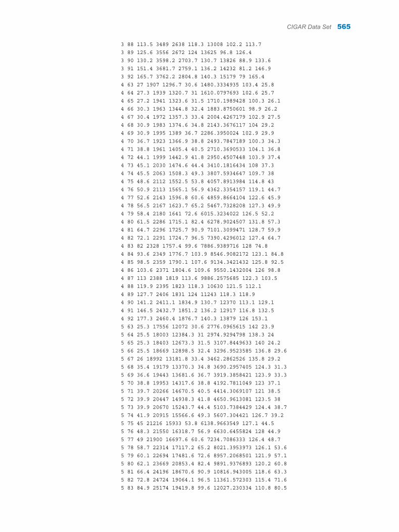
3 88 113.5 3489 2638 118.3 13008 102.2 113.7 3 89 125.6 3556 2672 124 13625 96.8 126.4 3 90 130.2 3598.2 2703.7 130.7 13826 88.9 133.6 3 91 151.4 3681.7 2759.1 136.2 14232 81.2 146.9 3 92 165.7 3762.2 2804.8 140.3 15179 79 165.4 4 63 27 1907 1296.7 30.6 1480.3334935 103.4 25.8 4 64 27.3 1939 1320.7 31 1610.0797693 102.6 25.7 4 65 27.2 1941 1323.6 31.5 1710.1989428 100.3 26.1 4 66 30.3 1963 1344.8 32.4 1883.8750601 98.9 26.2 4 67 30.4 1972 1357.3 33.4 2004.4267179 102.9 27.5 4 68 30.9 1983 1374.6 34.8 2143.3676117 104 29.2 4 69 30.9 1995 1389 36.7 2286.3950024 102.9 29.9 4 70 36.7 1923 1366.9 38.8 2493.7847189 100.3 34.3 4 71 38.8 1961 1405.4 40.5 2710.3690533 104.1 36.8 4 72 44.1 1999 1442.9 41.8 2950.4507448 103.9 37.4 4 73 45.1 2030 1474.6 44.4 3410.1816434 108 37.3 4 74 45.5 2063 1508.3 49.3 3807.5934647 109.7 38 4 75 48.6 2112 1552.5 53.8 4057.8913984 114.8 43 4 76 50.9 2113 1565.1 56.9 4362.3354157 119.1 44.7 4 77 52.6 2143 1596.8 60.6 4859.8664104 122.6 45.9 4 78 56.5 2167 1623.7 65.2 5467.7328208 127.3 49.9 4 79 58.4 2180 1641 72.6 6015.3234022 126.5 52.2 4 80 61.5 2286 1715.1 82.4 6278.9024507 131.8 57.3 4 81 64.7 2296 1725.7 90.9 7101.3099471 128.7 59.9 4 82 72.1 2291 1724.7 96.5 7390.4296012 127.4 64.7 4 83 82 2328 1757.4 99.6 7886.9389716 128 74.8 4 84 93.6 2349 1776.7 103.9 8546.9082172 123.1 84.8 4 85 98.5 2359 1790.1 107.6 9134.3421432 125.8 92.5 4 86 103.6 2371 1804.6 109.6 9550.1432004 126 98.8 4 87 113 2388 1819 113.6 9886.2575685 122.3 103.5 4 88 119.9 2395 1823 118.3 10630 121.5 112.1 4 89 127.7 2406 1831 124 11243 118.3 118.9 4 90 141.2 2411.1 1834.9 130.7 12370 113.1 129.1 4 91 146.5 2432.7 1851.2 136.2 12917 116.8 132.5 4 92 177.3 2460.4 1876.7 140.3 13879 126 153.1 5 63 25.3 17556 12072 30.6 2776.0965615 142 23.9 5 64 25.5 18003 12384.3 31 2974.9294798 138.3 24 5 65 25.3 18403 12673.3 31.5 3107.8449633 140 24.2 5 66 25.5 18669 12898.5 32.4 3296.9523585 136.8 29.6 5 67 26 18992 13181.8 33.4 3462.2862526 135.8 29.2 5 68 35.4 19179 13370.3 34.8 3690.2957405 124.3 31.3 5 69 36.6 19443 13681.6 36.7 3919.3858421 123.9 33.3 5 70 38.8 19953 14317.6 38.8 4192.7811049 123 37.1 5 71 39.7 20266 14670.5 40.5 4414.3069107 121 38.5 5 72 39.9 20447 14938.3 41.8 4650.9613081 123.5 38 5 73 39.9 20670 15243.7 44.4 5103.7384429 124.4 38.7 5 74 41.9 20915 15566.6 49.3 5607.304421 126.7 39.2 5 75 45 21216 15933 53.8 6138.9663549 127.1 44.5 5 76 48.3 21550 16318.7 56.9 6630.6455824 128 44.9 5 77 49 21900 16697.6 60.6 7234.7086333 126.4 48.7 5 78 58.7 22314 17117.2 65.2 8021.3953973 126.1 53.6 5 79 60.1 22694 17481.6 72.6 8957.2068501 121.9 57.1 5 80 62.1 23669 20853.4 82.4 9891.9376893 120.2 60.8 5 81 66.4 24196 18670.6 90.9 10816.943005 118.6 63.3 5 82 72.8 24724 19064.1 96.5 11361.572303 115.4 71.6 5 83 84.9 25174 19419.8 99.6 12027.230334 110.8 80.5
CIGAR Data Set 565
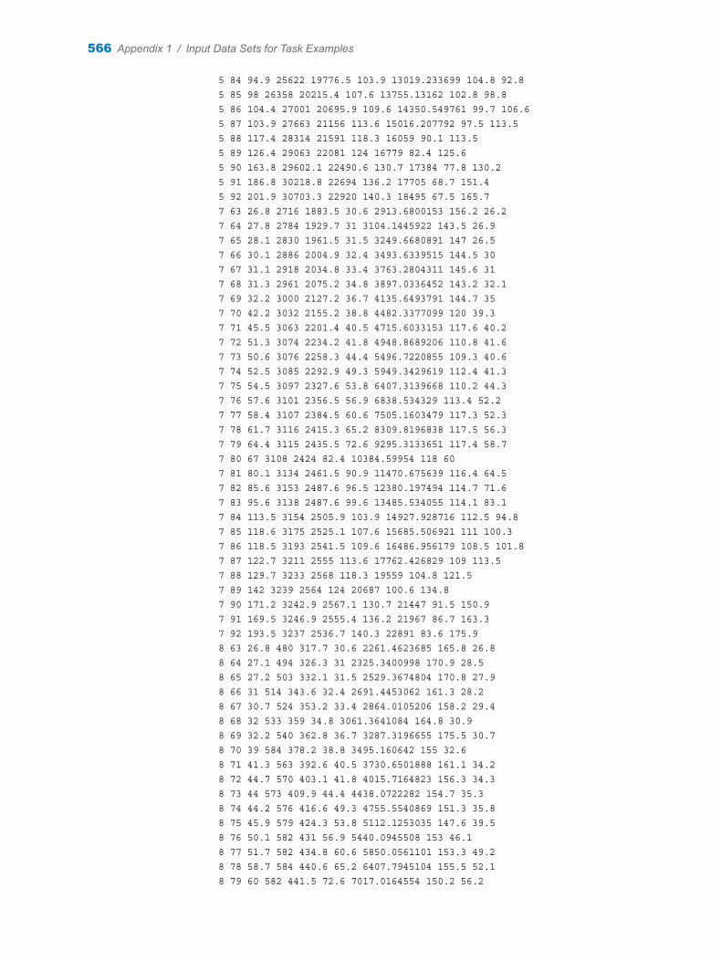
5 84 94.9 25622 19776.5 103.9 13019.233699 104.8 92.8 5 85 98 26358 20215.4 107.6 13755.13162 102.8 98.8 5 86 104.4 27001 20695.9 109.6 14350.549761 99.7 106.6 5 87 103.9 27663 21156 113.6 15016.207792 97.5 113.5 5 88 117.4 28314 21591 118.3 16059 90.1 113.5 5 89 126.4 29063 22081 124 16779 82.4 125.6 5 90 163.8 29602.1 22490.6 130.7 17384 77.8 130.2 5 91 186.8 30218.8 22694 136.2 17705 68.7 151.4 5 92 201.9 30703.3 22920 140.3 18495 67.5 165.7 7 63 26.8 2716 1883.5 30.6 2913.6800153 156.2 26.2 7 64 27.8 2784 1929.7 31 3104.1445922 143.5 26.9 7 65 28.1 2830 1961.5 31.5 3249.6680891 147 26.5 7 66 30.1 2886 2004.9 32.4 3493.6339515 144.5 30 7 67 31.1 2918 2034.8 33.4 3763.2804311 145.6 31 7 68 31.3 2961 2075.2 34.8 3897.0336452 143.2 32.1 7 69 32.2 3000 2127.2 36.7 4135.6493791 144.7 35 7 70 42.2 3032 2155.2 38.8 4482.3377099 120 39.3 7 71 45.5 3063 2201.4 40.5 4715.6033153 117.6 40.2 7 72 51.3 3074 2234.2 41.8 4948.8689206 110.8 41.6 7 73 50.6 3076 2258.3 44.4 5496.7220855 109.3 40.6 7 74 52.5 3085 2292.9 49.3 5949.3429619 112.4 41.3 7 75 54.5 3097 2327.6 53.8 6407.3139668 110.2 44.3 7 76 57.6 3101 2356.5 56.9 6838.534329 113.4 52.2 7 77 58.4 3107 2384.5 60.6 7505.1603479 117.3 52.3 7 78 61.7 3116 2415.3 65.2 8309.8196838 117.5 56.3 7 79 64.4 3115 2435.5 72.6 9295.3133651 117.4 58.7 7 80 67 3108 2424 82.4 10384.59954 118 60 7 81 80.1 3134 2461.5 90.9 11470.675639 116.4 64.5 7 82 85.6 3153 2487.6 96.5 12380.197494 114.7 71.6 7 83 95.6 3138 2487.6 99.6 13485.534055 114.1 83.1 7 84 113.5 3154 2505.9 103.9 14927.928716 112.5 94.8 7 85 118.6 3175 2525.1 107.6 15685.506921 111 100.3 7 86 118.5 3193 2541.5 109.6 16486.956179 108.5 101.8 7 87 122.7 3211 2555 113.6 17762.426829 109 113.5 7 88 129.7 3233 2568 118.3 19559 104.8 121.5 7 89 142 3239 2564 124 20687 100.6 134.8 7 90 171.2 3242.9 2567.1 130.7 21447 91.5 150.9 7 91 169.5 3246.9 2555.4 136.2 21967 86.7 163.3 7 92 193.5 3237 2536.7 140.3 22891 83.6 175.9 8 63 26.8 480 317.7 30.6 2261.4623685 165.8 26.8 8 64 27.1 494 326.3 31 2325.3400998 170.9 28.5 8 65 27.2 503 332.1 31.5 2529.3674804 170.8 27.9 8 66 31 514 343.6 32.4 2691.4453062 161.3 28.2 8 67 30.7 524 353.2 33.4 2864.0105206 158.2 29.4 8 68 32 533 359 34.8 3061.3641084 164.8 30.9 8 69 32.2 540 362.8 36.7 3287.3196655 175.5 30.7 8 70 39 584 378.2 38.8 3495.160642 155 32.6 8 71 41.3 563 392.6 40.5 3730.6501888 161.1 34.2 8 72 44.7 570 403.1 41.8 4015.7164823 156.3 34.3 8 73 44 573 409.9 44.4 4438.0722282 154.7 35.3 8 74 44.2 576 416.6 49.3 4755.5540869 151.3 35.8 8 75 45.9 579 424.3 53.8 5112.1253035 147.6 39.5 8 76 50.1 582 431 56.9 5440.0945508 153 46.1 8 77 51.7 582 434.8 60.6 5850.0561101 153.3 49.2 8 78 58.7 584 440.6 65.2 6407.7945104 155.5 52.1 8 79 60 582 441.5 72.6 7017.0164554 150.2 56.2
566 Appendix 1 / Input Data Sets for Task Examples
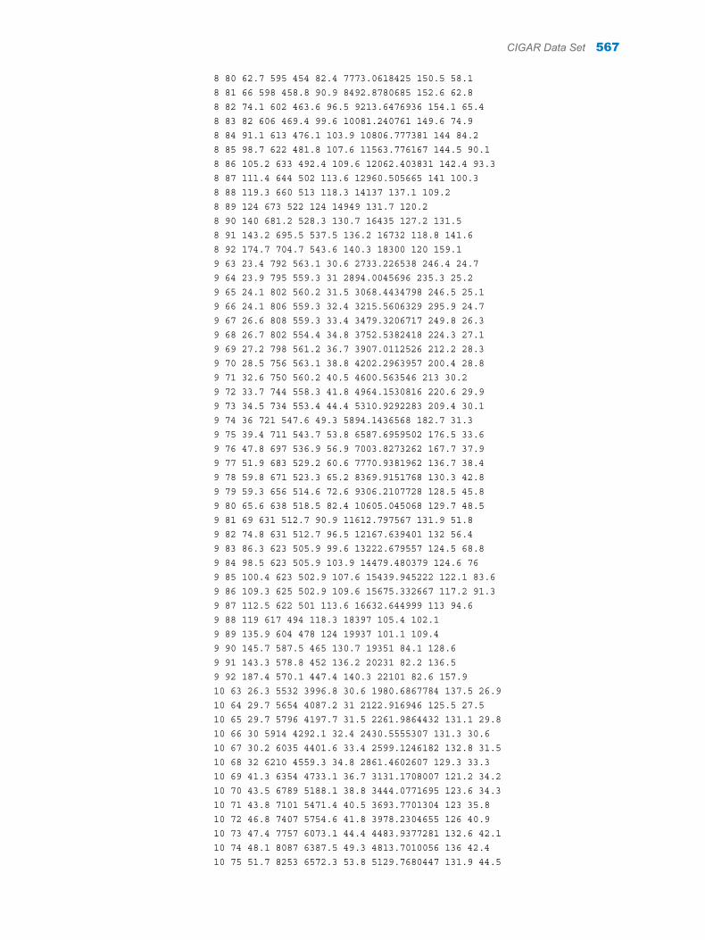
8 80 62.7 595 454 82.4 7773.0618425 150.5 58.1 8 81 66 598 458.8 90.9 8492.8780685 152.6 62.8 8 82 74.1 602 463.6 96.5 9213.6476936 154.1 65.4 8 83 82 606 469.4 99.6 10081.240761 149.6 74.9 8 84 91.1 613 476.1 103.9 10806.777381 144 84.2 8 85 98.7 622 481.8 107.6 11563.776167 144.5 90.1 8 86 105.2 633 492.4 109.6 12062.403831 142.4 93.3 8 87 111.4 644 502 113.6 12960.505665 141 100.3 8 88 119.3 660 513 118.3 14137 137.1 109.2 8 89 124 673 522 124 14949 131.7 120.2 8 90 140 681.2 528.3 130.7 16435 127.2 131.5 8 91 143.2 695.5 537.5 136.2 16732 118.8 141.6 8 92 174.7 704.7 543.6 140.3 18300 120 159.1 9 63 23.4 792 563.1 30.6 2733.226538 246.4 24.7 9 64 23.9 795 559.3 31 2894.0045696 235.3 25.2 9 65 24.1 802 560.2 31.5 3068.4434798 246.5 25.1 9 66 24.1 806 559.3 32.4 3215.5606329 295.9 24.7 9 67 26.6 808 559.3 33.4 3479.3206717 249.8 26.3 9 68 26.7 802 554.4 34.8 3752.5382418 224.3 27.1 9 69 27.2 798 561.2 36.7 3907.0112526 212.2 28.3 9 70 28.5 756 563.1 38.8 4202.2963957 200.4 28.8 9 71 32.6 750 560.2 40.5 4600.563546 213 30.2 9 72 33.7 744 558.3 41.8 4964.1530816 220.6 29.9 9 73 34.5 734 553.4 44.4 5310.9292283 209.4 30.1 9 74 36 721 547.6 49.3 5894.1436568 182.7 31.3 9 75 39.4 711 543.7 53.8 6587.6959502 176.5 33.6 9 76 47.8 697 536.9 56.9 7003.8273262 167.7 37.9 9 77 51.9 683 529.2 60.6 7770.9381962 136.7 38.4 9 78 59.8 671 523.3 65.2 8369.9151768 130.3 42.8 9 79 59.3 656 514.6 72.6 9306.2107728 128.5 45.8 9 80 65.6 638 518.5 82.4 10605.045068 129.7 48.5 9 81 69 631 512.7 90.9 11612.797567 131.9 51.8 9 82 74.8 631 512.7 96.5 12167.639401 132 56.4 9 83 86.3 623 505.9 99.6 13222.679557 124.5 68.8 9 84 98.5 623 505.9 103.9 14479.480379 124.6 76 9 85 100.4 623 502.9 107.6 15439.945222 122.1 83.6 9 86 109.3 625 502.9 109.6 15675.332667 117.2 91.3 9 87 112.5 622 501 113.6 16632.644999 113 94.6 9 88 119 617 494 118.3 18397 105.4 102.1 9 89 135.9 604 478 124 19937 101.1 109.4 9 90 145.7 587.5 465 130.7 19351 84.1 128.6 9 91 143.3 578.8 452 136.2 20231 82.2 136.5 9 92 187.4 570.1 447.4 140.3 22101 82.6 157.9 10 63 26.3 5532 3996.8 30.6 1980.6867784 137.5 26.9 10 64 29.7 5654 4087.2 31 2122.916946 125.5 27.5 10 65 29.7 5796 4197.7 31.5 2261.9864432 131.1 29.8 10 66 30 5914 4292.1 32.4 2430.5555307 131.3 30.6 10 67 30.2 6035 4401.6 33.4 2599.1246182 132.8 31.5 10 68 32 6210 4559.3 34.8 2861.4602607 129.3 33.3 10 69 41.3 6354 4733.1 36.7 3131.1708007 121.2 34.2 10 70 43.5 6789 5188.1 38.8 3444.0771695 123.6 34.3 10 71 43.8 7101 5471.4 40.5 3693.7701304 123 35.8 10 72 46.8 7407 5754.6 41.8 3978.2304655 126 40.9 10 73 47.4 7757 6073.1 44.4 4483.9377281 132.6 42.1 10 74 48.1 8087 6387.5 49.3 4813.7010056 136 42.4 10 75 51.7 8253 6572.3 53.8 5129.7680447 131.9 44.5
CIGAR Data Set 567
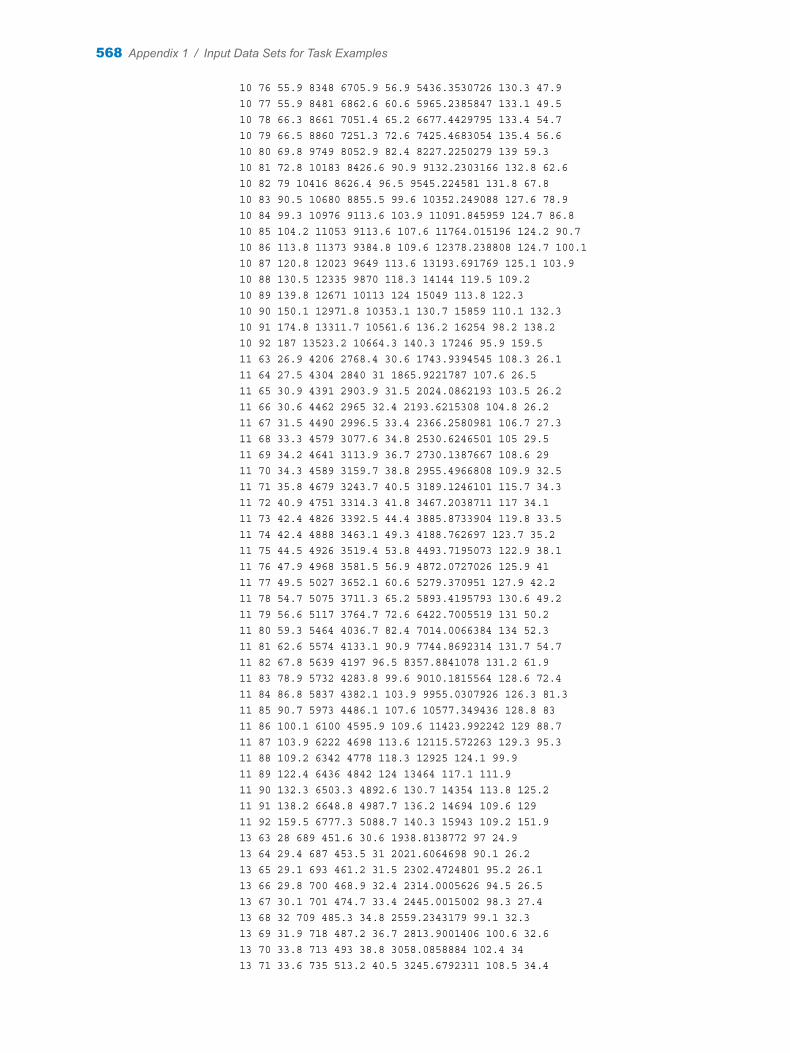
10 76 55.9 8348 6705.9 56.9 5436.3530726 130.3 47.9 10 77 55.9 8481 6862.6 60.6 5965.2385847 133.1 49.5 10 78 66.3 8661 7051.4 65.2 6677.4429795 133.4 54.7 10 79 66.5 8860 7251.3 72.6 7425.4683054 135.4 56.6 10 80 69.8 9749 8052.9 82.4 8227.2250279 139 59.3 10 81 72.8 10183 8426.6 90.9 9132.2303166 132.8 62.6 10 82 79 10416 8626.4 96.5 9545.224581 131.8 67.8 10 83 90.5 10680 8855.5 99.6 10352.249088 127.6 78.9 10 84 99.3 10976 9113.6 103.9 11091.845959 124.7 86.8 10 85 104.2 11053 9113.6 107.6 11764.015196 124.2 90.7 10 86 113.8 11373 9384.8 109.6 12378.238808 124.7 100.1 10 87 120.8 12023 9649 113.6 13193.691769 125.1 103.9 10 88 130.5 12335 9870 118.3 14144 119.5 109.2 10 89 139.8 12671 10113 124 15049 113.8 122.3 10 90 150.1 12971.8 10353.1 130.7 15859 110.1 132.3 10 91 174.8 13311.7 10561.6 136.2 16254 98.2 138.2 10 92 187 13523.2 10664.3 140.3 17246 95.9 159.5 11 63 26.9 4206 2768.4 30.6 1743.9394545 108.3 26.1 11 64 27.5 4304 2840 31 1865.9221787 107.6 26.5 11 65 30.9 4391 2903.9 31.5 2024.0862193 103.5 26.2 11 66 30.6 4462 2965 32.4 2193.6215308 104.8 26.2 11 67 31.5 4490 2996.5 33.4 2366.2580981 106.7 27.3 11 68 33.3 4579 3077.6 34.8 2530.6246501 105 29.5 11 69 34.2 4641 3113.9 36.7 2730.1387667 108.6 29 11 70 34.3 4589 3159.7 38.8 2955.4966808 109.9 32.5 11 71 35.8 4679 3243.7 40.5 3189.1246101 115.7 34.3 11 72 40.9 4751 3314.3 41.8 3467.2038711 117 34.1 11 73 42.4 4826 3392.5 44.4 3885.8733904 119.8 33.5 11 74 42.4 4888 3463.1 49.3 4188.762697 123.7 35.2 11 75 44.5 4926 3519.4 53.8 4493.7195073 122.9 38.1 11 76 47.9 4968 3581.5 56.9 4872.0727026 125.9 41 11 77 49.5 5027 3652.1 60.6 5279.370951 127.9 42.2 11 78 54.7 5075 3711.3 65.2 5893.4195793 130.6 49.2 11 79 56.6 5117 3764.7 72.6 6422.7005519 131 50.2 11 80 59.3 5464 4036.7 82.4 7014.0066384 134 52.3 11 81 62.6 5574 4133.1 90.9 7744.8692314 131.7 54.7 11 82 67.8 5639 4197 96.5 8357.8841078 131.2 61.9 11 83 78.9 5732 4283.8 99.6 9010.1815564 128.6 72.4 11 84 86.8 5837 4382.1 103.9 9955.0307926 126.3 81.3 11 85 90.7 5973 4486.1 107.6 10577.349436 128.8 83 11 86 100.1 6100 4595.9 109.6 11423.992242 129 88.7 11 87 103.9 6222 4698 113.6 12115.572263 129.3 95.3 11 88 109.2 6342 4778 118.3 12925 124.1 99.9 11 89 122.4 6436 4842 124 13464 117.1 111.9 11 90 132.3 6503.3 4892.6 130.7 14354 113.8 125.2 11 91 138.2 6648.8 4987.7 136.2 14694 109.6 129 11 92 159.5 6777.3 5088.7 140.3 15943 109.2 151.9 13 63 28 689 451.6 30.6 1938.8138772 97 24.9 13 64 29.4 687 453.5 31 2021.6064698 90.1 26.2 13 65 29.1 693 461.2 31.5 2302.4724801 95.2 26.1 13 66 29.8 700 468.9 32.4 2314.0005626 94.5 26.5 13 67 30.1 701 474.7 33.4 2445.0015002 98.3 27.4 13 68 32 709 485.3 34.8 2559.2343179 99.1 32.3 13 69 31.9 718 487.2 36.7 2813.9001406 100.6 32.6 13 70 33.8 713 493 38.8 3058.0858884 102.4 34 13 71 33.6 735 513.2 40.5 3245.6792311 108.5 34.4
568 Appendix 1 / Input Data Sets for Task Examples
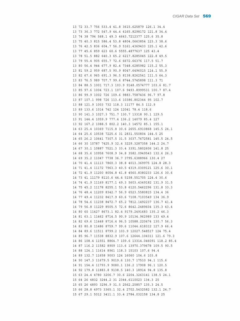
13 72 33.7 756 533.4 41.8 3615.625879 126.1 34.4 13 73 36.3 772 547.9 44.4 4165.8298172 121.8 34.4 13 74 38 794 568.1 49.3 4643.7212377 125.6 35.8 13 75 40.3 815 586.4 53.8 4804.0663854 123.3 38.6 13 76 42.5 836 604.7 56.9 5161.4369433 125.1 42.6 13 77 45.6 859 623 60.6 5555.4877637 125 43.4 13 78 51.5 882 640.3 65.2 6217.8285045 122.8 49.5 13 79 55.4 905 655.7 72.6 6672.66376 117.5 51.7 13 80 56.4 944 677.9 82.4 7348.6285982 115.2 55.3 13 81 59.2 959 687.5 90.9 8047.6496015 114.1 55.9 13 82 67.6 965 691.3 96.5 8138.8262541 111.5 64.3 13 83 76.5 989 707.7 99.6 8744.5745898 111.3 71 13 84 88.5 1001 717.3 103.9 9148.0574777 103.6 81.7 13 85 97.6 1004 723.1 107.6 9493.8999531 100.7 87.4 13 86 99.9 1002 726 109.6 9883.7587436 96.7 97.8 13 87 107.1 998 726 113.6 10386.802344 95 102.7 13 88 121.9 1003 732 118.3 11177 84.5 112.9 13 89 133.6 1014 742 124 12041 78.4 118.6 13 90 141.3 1027.3 751.7 130.7 13318 90.1 129.5 13 91 144.4 1059.9 777.4 136.2 14079 85.4 127 13 92 167.2 1088.5 802.2 140.3 14572 85.1 155.1 14 63 25.4 10369 7115.8 30.6 2655.6910868 145.5 24.1 14 64 25.6 10538 7225.6 31 2831.550804 144.5 25 14 65 26.2 10641 7307.5 31.5 3037.7672581 145.5 24.5 14 66 30 10787 7425.9 32.4 3229.3287358 144.2 24.7 14 67 30.1 10887 7521.3 33.4 3391.5802606 141.8 25 14 68 35.6 10958 7608.9 34.8 3582.0949543 132.6 26.3 14 69 35.2 11047 7738 36.7 3795.6388966 130.4 27 14 70 41.4 11113 7860.3 38.8 4013.369975 124.8 28.3 14 71 41.4 11172 7963.3 40.5 4319.0309121 125.6 30.1 14 72 41.9 11200 8054.8 41.8 4560.8380233 126.6 30.6 14 73 41 11179 8110.6 44.4 5158.551705 124.4 30.6 14 74 41.9 11169 8177.1 49.3 5603.4349182 131.9 31.5 14 75 45.2 11178 8255.1 53.8 6120.5462296 131.8 33.3 14 76 48.4 11209 8342.7 56.9 6523.5580815 134.4 36 14 77 49.4 11232 8417.9 60.6 7108.7103549 134 36.9 14 78 54.6 11238 8472.7 65.2 7812.1492237 136.7 41.4 14 79 56.8 11229 8505.5 72.6 8642.2489604 135.3 43.4 14 80 60 11427 8673.1 82.4 9179.2491683 135.2 46.3 14 81 63.1 11462 8714.5 90.9 10134.962989 133 49.4 14 82 69.6 11448 8716.4 96.5 10588.220474 130.7 56.3 14 83 80.8 11486 8759.7 99.6 11044.618312 127.9 66.4 14 84 89.6 11511 8799.2 103.9 12027.548517 124 75.4 14 85 96.7 11538 8832.9 107.6 12644.104311 121.6 79.3 14 86 108.4 11551 8864.7 109.6 13314.046091 118.2 85.4 14 87 116.2 11582 8909 113.6 13970.379678 109.5 90.5 14 88 124.1 11614 8961 118.3 15103 107.6 94.4 14 89 132.7 11658 9003 124 16060 104.6 103.8 14 90 147.3 11679.5 9019.6 130.7 17510 94.1 115.6 14 91 154.4 11793.9 9080.1 136.2 17908 96.1 120.5 14 92 179.8 11883.8 9138.5 140.3 18914 94.8 135.8 15 63 24.4 4780 3206.7 30.6 2204.3263141 138.5 24.1 15 64 26 4832 3244.2 31 2344.6110023 134.3 25 15 65 26 4893 3296.9 31.5 2562.25857 135.3 24.5 15 66 28.8 4973 3365.1 32.4 2702.5432582 132.1 24.7 15 67 29.1 5012 3411.1 33.4 2784.032158 134.8 25
CIGAR Data Set 569
15 68 29.8 5065 3472.5 34.8 2970.7345739 134.3 26.3 15 69 29.7 5118 3514.8 36.7 3194.5711721 132.9 27 15 70 30.6 5193 3616.5 38.8 3304.9422135 134.6 28.3 15 71 32.2 5239 3681.7 40.5 3570.039014 139.3 30.1 15 72 32.5 5278 3743.1 41.8 3812.4427032 149.2 30.6 15 73 32.9 5304 3794.9 44.4 4427.2197192 156 30.6 15 74 34.5 5318 3840 49.3 4611.859125 159.6 31.5 15 75 36.7 5312 3869.8 53.8 5024.4611492 162.4 33.3 15 76 38.7 5326 3912 56.9 5521.6465883 166.6 36 15 77 40.6 5352 3960 60.6 6012.6429971 173 36.9 15 78 50 5387 4013.7 65.2 6663.5226902 150.9 41.4 15 79 52.5 5400 4045.4 72.6 7358.7571009 148.9 43.4 15 80 53.7 5490 4103.9 82.4 7760.0125694 146.9 46.3 15 81 58.3 5468 4102 90.9 8407.7977473 148.5 49.4 15 82 65.1 5471 4115.4 96.5 8612.0357493 147.7 56.3 15 83 75.7 5479 4134.6 99.6 9060.7404505 143 66.4 15 84 85.2 5498 4164.4 103.9 10077.80444 137.8 75.4 15 85 88.8 5500 4186.4 107.6 10502.784525 135.3 79.3 15 86 93.6 5503 4211.4 109.6 11140.254652 137.6 85.4 15 87 100.1 5531 4244 113.6 11803.512406 134 90.5 15 88 109.3 5556 4275 118.3 12638 134 94.4 15 89 119 5593 4301 124 13451 132.5 103.8 15 90 130.8 5613.2 4316.6 130.7 14441 128.3 115.6 15 91 135.8 5680.1 4373.5 136.2 14773 127.2 120.5 15 92 153.5 5732.7 4430.4 140.3 15882 128.2 135.8 16 63 26.4 2758 1880.7 30.6 2153.014454 114.9 25.4 16 64 27.9 2763 1889.4 31 2280.5627037 109.7 25.6 16 65 28.1 2758 1897.1 31.5 2537.6999749 116 26.1 16 66 31.6 2764 1912.5 32.4 2722.3898404 108.2 26.2 16 67 32 2772 1930.8 33.4 2744.8383324 113.7 27.5 16 68 36.3 2775 1950.1 34.8 2918.3039519 109.2 29.2 16 69 36 2781 1963.6 36.7 3165.2373632 107.9 29.9 16 70 37.7 2825 2000.2 38.8 3369.3145626 108.5 33.9 16 71 38.5 2849 2036.8 40.5 3507.0666722 108.4 34.7 16 72 41.9 2856 2062.8 41.8 3892.7725792 109.4 37.7 16 73 41.9 2858 2084 44.4 4829.4869246 110.6 37.7 16 74 43.2 2861 2108.1 49.3 4793.7734147 116.1 38 16 75 45.4 2873 2137 53.8 5289.6810093 120.5 42.8 16 76 47.8 2894 2172.7 56.9 5794.7720779 124.4 44.7 16 77 49.4 2903 2195.8 60.6 6047.8278052 125.5 45.9 16 78 54.6 2906 2213.1 65.2 7016.1741165 127.1 49.9 16 79 56.4 2902 2219.9 72.6 7617.1814688 124.2 52.2 16 80 58.8 2913 2213.1 82.4 7957.9903918 124.6 57.3 16 81 61.4 2899 2206.4 90.9 8951.8463531 132.9 59.9 16 82 72.8 2905 2212.2 96.5 9118.1692706 116.2 64.7 16 83 84 2905 2216 99.6 9124.2915866 115.6 74.8 16 84 93.3 2910 2218.9 103.9 10180.391094 111.2 84.8 16 85 99.5 2880 2209.3 107.6 10668.1356 109.4 92.3 16 86 104.8 2850 2195.8 109.6 11155.880107 104.1 101.9 16 87 117.1 2834 2190 113.6 11623.216894 101.1 108.5 16 88 124.2 2834 2203 118.3 12213 100.2 114.6 16 89 145.1 2840 2209 124 13138 94.4 118.9 16 90 149.6 2846.1 2213.8 130.7 14647 95.4 129.1 16 91 155.4 2864.6 2228.3 136.2 14873 97.1 132.5 16 92 178.5 2882 2238.7 140.3 16089 95.2 153.1 17 63 25.8 2261 1550.4 30.6 2148.6675472 115.8 25.8
570 Appendix 1 / Input Data Sets for Task Examples
17 64 25.6 2237 1537.8 31 2316.5973895 111.2 25.7 17 65 28.1 2248 1552.3 31.5 2488.6994018 107.8 26.1 17 66 30.5 2275 1582.3 32.4 2639.9405641 101.7 26.2 17 67 31 2281 1597.8 33.4 2768.2347914 101.2 27.5 17 68 32.4 2291 1622 34.8 2945.5520162 100.1 29.2 17 69 32.6 2321 1656.9 36.7 3163.5478984 102.6 29.9 17 70 34.2 2249 1624.9 38.8 3411.7920131 114 33.9 17 71 38.9 2247 1641.4 40.5 3717.4034652 102.8 34.7 17 72 38.8 2259 1665.6 41.8 4125.2330821 111 37.7 17 73 39.3 2269 1687.9 44.4 4790.6941963 115.2 37.7 17 74 40.2 2275 1706.3 49.3 5095.2626059 118.6 38 17 75 42.7 2287 1730.5 53.8 5498.9200528 123.4 43.5 17 76 46.6 2309 1760.5 56.9 5587.5786652 127.7 44.7 17 77 48.1 2331 1787.6 60.6 6407.4100691 127.9 45.9 17 78 52.6 2347 1810.8 65.2 7177.1754331 127.1 49.9 17 79 54.8 2369 1832.2 72.6 8258.8105042 126.4 52.2 17 80 58.3 2363 1814.7 82.4 8365.2008391 127.1 57.3 17 81 59.8 2383 1828.3 90.9 9461.4385052 132 59.9 17 82 65.1 2408 1843.8 96.5 10019.466242 130.9 64.7 17 83 77 2425 1856.4 99.6 10400.176754 127.6 74.8 17 84 91 2438 1867 103.9 11277.375495 121.7 84.8 17 85 97.5 2449 1873.8 107.6 11843.747572 115.7 93.7 17 86 103 2459 1887.3 109.6 12517.553026 109.4 101.9 17 87 114.5 2476 1898 113.6 12827.336648 105.2 108.5 17 88 123.9 2495 1912 118.3 13425 103.2 114.6 17 89 136.5 2513 1920 124 14103 96.5 118.9 17 90 145.8 2518.1 1923.9 130.7 15398 94.3 129.1 17 91 145.7 2535.4 1932.1 136.2 15849 91.8 132.5 17 92 174.2 2563.8 1913 140.3 16982 90 153.1 18 63 24.1 3121 2106.7 30.6 1724.5821178 126.3 24.4 18 64 25 3163 2142.2 31 1792.8512029 127 25.2 18 65 24.5 3173 2157.6 31.5 1935.6911347 128.7 25.1 18 66 24.7 3181 2176.8 32.4 2089.0340027 134 24.7 18 67 25 3201 2207.5 33.4 2237.1254025 139.3 26.3 18 68 26.3 3224 2242.1 34.8 2405.1723811 142.8 27.1 18 69 27 3232 2256.5 36.7 2587.9234704 146.3 28.3 18 70 28.3 3219 2270 38.8 2812.6863042 155.8 28.8 18 71 30.1 3280 2330.5 40.5 3006.9906232 163.5 30.2 18 72 30.6 3303 2360.3 41.8 3239.1055124 179.4 29.9 18 73 30.6 3325 2396.8 44.4 3653.9714908 201.9 30.1 18 74 31.5 3356 2440 49.3 4052.0327714 212.4 31.3 18 75 33.3 3392 2484.2 53.8 4380.7746732 223 33.6 18 76 36 3439 2537 56.9 4802.992707 230.9 37.9 18 77 36.9 3468 2574.5 60.6 5232.562796 229.4 38.4 18 78 41.4 3490 2603.3 65.2 5753.5084296 224.7 42.8 18 79 43.4 3527 2641.7 72.6 6409.9419398 214.9 45.8 18 80 46.3 3661 2737.8 82.4 6775.4441182 215.3 48.5 18 81 49.4 3662 2745.5 90.9 7506.4484751 209.7 51.8 18 82 56.3 3667 2757 96.5 7988.5332449 210.6 56.4 18 83 66.4 3714 2800.2 99.6 8272.1125213 201.1 68.8 18 84 75.4 3723 2812.7 103.9 9062.9836143 183.2 76 18 85 79.3 3728 2829.1 107.6 9282.4949801 182.4 83.6 18 86 85.4 3726 2841.6 109.6 9722.5680053 179.8 91.3 18 87 90.5 3727 2855 113.6 10328.587422 171.2 94.6 18 88 94.4 3727 2867 118.3 11089 173.2 102.1 18 89 103.8 3727 2874 124 11873 171.6 109.4
CIGAR Data Set 571
18 90 115.6 3735.1 2880.3 130.7 12879 182.5 128.6 18 91 120.5 3763.5 2903.6 136.2 13338 170.8 132.5 18 92 135.8 3806.1 2942.1 140.3 14664 167.6 153.1 19 63 30.1 3410 2194 30.6 1675.9379252 114 27 19 64 30.1 3493 2253.6 31 1782.5702302 114 27.3 19 65 30.3 3560 2305.5 31.5 1910.3278032 117.5 27.2 19 66 30 3624 2363.2 32.4 2054.1808183 119.7 30.3 19 67 31.5 3663 2404.5 33.4 2236.2605089 120 30.4 19 68 32.5 3710 2455.5 34.8 2413.3103738 117.3 30.9 19 69 33.3 3745 2467 36.7 2511.8949576 115.9 30.9 19 70 34.3 3643 2467 38.8 2709.0641253 115.9 36.2 19 71 39.3 3696 2530.5 40.5 2877.0603038 119.8 37.5 19 72 40 3737 2580.5 41.8 3075.2354367 125.3 37.4 19 73 39.9 3753 2616 44.4 3410.2218287 126.7 37.3 19 74 41.6 3774 2658.3 49.3 3855.8643862 129.9 41.4 19 75 44.3 3829 2722.8 53.8 4252.2146519 133.6 43 19 76 48.1 3883 2781.4 56.9 4694.839314 139.6 46.4 19 77 48.9 3935 2839.1 60.6 5161.6071395 140 48.8 19 78 54.2 3978 2889.1 65.2 5786.3114922 142.7 53.6 19 79 57.1 4018 2933.3 72.6 6416.0456706 140.1 56.5 19 80 60 4204 3079.4 82.4 7284.1935875 143.8 59.7 19 81 62.6 4308 3160.2 90.9 8164.413086 144 63 19 82 70.3 4362 3200.6 96.5 8669.4075869 143.9 69.2 19 83 80.7 4438 3256.4 99.6 8984.2746761 133.7 78.6 19 84 90.7 4462 3274.6 103.9 9465.1260136 128.9 89 19 85 103 4485 3294.8 107.6 9747.8022183 125 96.4 19 86 105.1 4499 3313.1 109.6 9902.72085 121.2 103.6 19 87 117.8 4461 3290 113.6 10098.884053 116.5 113 19 88 120.4 4408 3250 118.3 10793 110.9 119.9 19 89 130.7 4382 3239 124 11348 103.6 125.8 19 90 143.4 4348 3213.9 130.7 12764 101.5 139.9 19 91 149.6 4381 3239.6 136.2 13349 107.2 142.7 19 92 178.1 4417 3274.6 140.3 14163 108.5 160.8 20 63 26.7 985 669.7 30.6 1878.7179278 138.4 24.2 20 64 26.8 984 668.7 31 2042.6400586 137.4 24.7 20 65 27.2 986 671.6 31.5 2212.948766 139.1 24.7 20 66 29.6 985 673.5 32.4 2356.6467378 135.1 25.9 20 67 30.3 982 674.5 33.4 2447.1232386 136 26.5 20 68 32 978 676.4 34.8 2613.1742282 135.6 29.9 20 69 33.4 978 680.2 36.7 2827.1245418 135.2 29.9 20 70 38 993 697.5 38.8 3103.8761913 128.5 31.4 20 71 38.8 1012 716.7 40.5 3280.5714751 133.2 34.1 20 72 41.5 1028 734 41.8 3507.2949418 136.5 36.1 20 73 41 1037 747.4 44.4 3870.2653743 138 36.9 20 74 41.8 1048 760.8 49.3 4234.3002362 142.1 37.9 20 75 46.7 1058 776.2 53.8 4492.9565855 140.7 40.8 20 76 49.9 1072 792.5 56.9 5028.3645842 144.9 43.9 20 77 50.9 1084 808.8 60.6 5440.2987701 145.6 45 20 78 55 1092 819.3 65.2 5882.0369797 143.9 49.7 20 79 54.5 1097 828.9 72.6 6445.1201434 138.5 53.2 20 80 59 1125 851 82.4 7097.6153783 141.2 55.3 20 81 62.9 1133 862.5 90.9 7850.1669789 138.9 58.4 20 82 69.7 1133 864.4 96.5 8341.9333713 139.5 67 20 83 80.8 1146 877.9 99.6 8962.4957237 135.4 74.7 20 84 93.7 1156 890.3 103.9 9851.2942901 135.5 90.5 20 85 98.1 1165 899.9 107.6 10501.660666 127.9 89.2
572 Appendix 1 / Input Data Sets for Task Examples
20 86 112.7 1172 908.6 109.6 11146.704895 119 100 20 87 121.2 1187 922 113.6 12056.79205 125 102 20 88 129 1205 940 118.3 13068 125 113.5 20 89 144.4 1222 953 124 14110 122.4 125.9 20 90 160.1 1230 959.2 130.7 14975 117.5 135.9 20 91 158.9 1237 963.3 136.2 15093 116.1 153.9 20 92 187.7 1237 968.3 140.3 16298 114.7 164.4 21 63 28.2 3351 2238 30.6 2312.3069668 122.7 23.4 21 64 28.5 3442 2299.3 31 2483.3969442 122.2 23.9 21 65 27.9 3534 2365.4 31.5 2629.6011066 121 24.1 21 66 28.2 3608 2425.8 32.4 2780.9898139 121 24.1 21 67 29.4 3680 2485.2 33.4 2967.6334256 121.7 26.3 21 68 30.9 3716 2523.6 34.8 3140.7972208 121.7 26.7 21 69 30.7 3765 2563.8 36.7 3384.4708249 122.3 27.2 21 70 32.6 3922 2723.9 38.8 3702.8018737 123.5 28.5 21 71 34.2 4011 2816.9 40.5 3968.2505659 126.7 30.2 21 72 34.3 4062 2884 41.8 4212.961079 133.2 29.9 21 73 35.3 4082 2933.8 44.4 4684.7546529 137.3 30.1 21 74 35.8 4099 2980.8 49.3 5073.5955106 144.8 31.3 21 75 39.5 4115 3028.7 53.8 5543.3152666 146.1 33.6 21 76 46.1 4123 3071.8 56.9 6029.6255659 137.1 37.9 21 77 49.2 4138 3114.9 60.6 6435.0569668 135.7 38.4 21 78 52.1 4148 3153.3 65.2 7184.7421403 134.1 42.8 21 79 56.2 4148 3181.1 72.6 7917.8367706 131.9 45.8 21 80 58.1 4216 3230.9 82.4 8888.3835513 131.5 48.5 21 81 62.8 4263 3287.5 90.9 9726.2059859 137.1 51.8 21 82 65.4 4265 3302.8 96.5 10426.11953 131.3 56.4 21 83 74.9 4304 3346.9 99.6 11464.065392 128.2 68.8 21 84 84.2 4349 3391.9 103.9 12555.930521 122.5 76 21 85 90.1 4391 3434.1 107.6 13494.333124 121.9 83.6 21 86 93.3 4461 3496.4 109.6 14247.129024 121.8 91.3 21 87 100.3 4535 3552 113.6 15111.911092 119.3 94.6 21 88 109.2 4622 3612 118.3 16491 115 102.1 21 89 120.2 4694 3658 124 17489 109 109.4 21 90 131.5 4747.6 3699.8 130.7 18172 102.8 128.6 21 91 141.6 4826.1 3737.4 136.2 18477 97.6 136.5 21 92 159.1 4871.8 3760.2 140.3 19746 91.7 157.9 22 63 28 5252 3669.4 30.6 2498.0022941 142.2 24.2 22 64 28.4 5287 3686.8 31 2653.9271915 138.7 24.7 22 65 28.4 5361 3740.8 31.5 2802.3762376 136.5 24.7 22 66 31 5403 3779.3 32.4 2983.932625 131.6 25.9 22 67 33.6 5434 3812.1 33.4 3187.916566 130.2 26.5 22 68 35.1 5438 3839.1 34.8 3401.5123159 128 29.9 22 69 35 5467 3914.3 36.7 3626.8558319 129.7 29.9 22 70 39.6 5689 4076.2 38.8 3931.2297754 124.3 31.4 22 71 41 5741 4151.4 40.5 4199.2924414 121.4 34.1 22 72 46 5767 4211.1 41.8 4442.7915962 117.9 36.1 22 73 46 5793 4274.8 44.4 4861.4392659 121.2 36.9 22 74 46.3 5789 4313.3 49.3 5272.6110843 124.3 37.9 22 75 49.4 5778 4350.9 53.8 5721.1621589 126.1 40.8 22 76 57.4 5769 4389.5 56.9 6115.2463173 116.9 43.9 22 77 57.3 5768 4432.8 60.6 6611.8564356 118.9 45 22 78 61.8 5771 4477.2 65.2 7274.0032601 120.5 49.7 22 79 64.5 5769 4513.8 72.6 8027.9962569 118.2 53.2 22 80 68.2 5737 4493.6 82.4 8940.0501087 120.5 55.3 22 81 70.8 5773 4552.3 90.9 9837.1522579 123.2 58.4
CIGAR Data Set 573
22 82 78.1 5781 4577.4 96.5 10820.760686 122.3 66.8 22 83 88.7 5767 4585.1 99.6 11715.726878 119.8 74.7 22 84 101.4 5798 4627.5 103.9 13018.660951 116 90.5 22 85 108.3 5823 4663.2 107.6 13860.228206 117.2 89.2 22 86 115 5834 4679.6 109.6 14869.468124 115.8 100 22 87 120.4 5855 4695 113.6 16086.963898 113.8 102 22 88 131.6 5889 4722 118.3 17690 111.7 113.5 22 89 148.6 5913 4726 124 18636 104.4 125.9 22 90 152.4 5913 4726 130.7 19051 99.4 135.9 22 91 163.3 5893.3 4678.8 136.2 19385 93.5 150.1 22 92 175.9 5895.3 4668 140.3 20822 90.5 164.4 23 63 28.8 8036 5265.5 30.6 2251.0006434 126.7 24.4 23 64 29.3 8161 5362.8 31 2462.5308457 125 26 23 65 28.7 8317 5494.4 31.5 2675.0588319 131.8 26 23 66 29.2 8496 5646.1 32.4 2845.6798913 134.5 26.3 23 67 30 8608 5758.7 33.4 2906.5447137 134.4 27 23 68 32 8673 5849.3 34.8 3126.0571878 134.2 29.8 23 69 31.9 8766 5892.2 36.7 3303.662735 133.4 29.7 23 70 33.7 8875 6064.9 38.8 3415.41454 128.6 30.6 23 71 39.2 8965 6198.4 40.5 3710.758596 126.1 32.2 23 72 40 9015 6301.4 41.8 4008.09822 131.4 32.5 23 73 40.2 9060 6398.7 44.4 4496.0145829 133.7 32.9 23 74 41.1 9096 6488.4 49.3 4812.3121024 138.8 34.5 23 75 44.4 9092 6553.3 53.8 5141.5808135 136.8 36.7 23 76 47.9 9100 6621.9 56.9 5686.3708628 138 38.7 23 77 48.3 9138 6704.9 60.6 6325.9503896 140.3 40.6 23 78 54 9181 6787.9 65.2 7044.3548502 141.8 50 23 79 57.2 9207 6849 72.6 7732.8257917 140.9 52.5 23 80 60.3 9262 6880.4 82.4 8329.5006076 140.7 53.7 23 81 61.8 9204 6871.9 90.9 9004.0025735 139.5 58.3 23 82 68 9109 6828 96.5 9337.2624205 137.3 65.1 23 83 87.7 9069 6828 99.6 10002.784331 128.3 75.7 23 84 97 9075 6864.2 103.9 11039.481879 128.2 85.2 23 85 101.4 9085 6913.8 107.6 11760.879691 126.6 88.8 23 86 106 9139 6992 109.6 12501.235399 126.5 93.6 23 87 111.4 9200 7055 113.6 13064.983344 122.1 100.1 23 88 122.2 9240 7090 118.3 13957.002216 121.1 108.4 23 89 133 9273 7108 124 14757 116.6 119 23 90 143.9 9315.1 7140.3 130.7 15560 114.4 130.8 23 91 144.9 9388.2 7183.5 136.2 15938 110.3 135.8 23 92 176.7 9457.4 7226.7 140.3 17154 107.6 153.5 24 63 28.7 3507 2314.2 30.6 2067.2509051 112.6 26.4 24 64 30.1 3529 2333.4 31 2157.0879797 104.7 27.9 24 65 30.2 3562 2367.9 31.5 2360.7186821 109.2 28.1 24 66 30.3 3585 2398.6 32.4 2527.416365 110.7 30.2 24 67 30.9 3625 2444.7 33.4 2669.1593049 114.4 30.5 24 68 32.7 3663 2493.6 34.8 2876.7827661 113.7 32.3 24 69 32.8 3700 2516.7 36.7 3071.429761 112.3 32.3 24 70 39.1 3805 2624.1 38.8 3331.9572773 104.3 37.3 24 71 40.1 3853 2690.3 40.5 3524.6078928 116.4 38.5 24 72 45.2 3870 2734.5 41.8 3757.186097 96.8 38.9 24 73 45.6 3891 2783.4 44.4 4514.8120927 106.8 39.4 24 74 47 3907 2829.4 49.3 4644.576756 110.6 39.9 24 75 49.4 3937 2885.1 53.8 4962.9992759 111.5 42.6 24 76 52.1 3970 2941.7 56.9 5312.365677 116.7 45 24 77 53.1 3996 2989.7 60.6 6025.0731354 117.2 46.4
574 Appendix 1 / Input Data Sets for Task Examples
24 78 57.9 4024 3033.8 65.2 6668.9055033 118.9 53.2 24 79 60.9 4060 3078.9 72.6 7378.6183925 118.3 54.1 24 80 63 4077 3079.9 82.4 8054.3928313 117.7 58.8 24 81 65.8 4094 3101.9 90.9 8895.8667632 120.8 61.4 24 82 71.7 4133 3130.7 96.5 9376.9942071 119.4 67.8 24 83 87.3 4144 3143.2 99.6 9884.0745836 113.2 77.9 24 84 99.2 4162 3166.2 103.9 11105.858798 110.8 89.8 24 85 101.5 4190 3196.9 107.6 11676.823316 113 92.3 24 86 116.3 4213 3224.7 109.6 12407.49819 104.3 104.2 24 87 120.1 4246 3266 113.6 12961.493483 108.8 110.3 24 88 141.7 4307 3312 118.3 13785 94.1 123.3 24 89 152.5 4353 3339 124 14771 92.3 130.1 24 90 162.3 4390.1 3367.5 130.7 15553 90.7 138.9 24 91 173.9 4447.3 3406 136.2 15869 86.2 150.3 24 92 197.7 4495.5 3440.5 140.3 17255 83.8 160 25 63 30.5 2291 1460.9 30.6 1322.5729775 83.9 26.1 25 64 30.4 2304 1472.4 31 1383.3694746 86.1 27.3 25 65 31.4 2309 1483.8 31.5 1496.9891576 83.5 27.2 25 66 31.8 2339 1516.1 32.4 1616.588824 86.9 29.5 25 67 31.6 2344 1530.4 33.4 1760.1084237 88.1 29.6 25 68 33.9 2349 1547.5 34.8 1919.5746455 89 30.9 25 69 34.8 2360 1541.8 36.7 2069.0742285 91 30.9 25 70 36.2 2216 1490.4 38.8 2243.4904087 93.4 34.3 25 71 37.5 2253 1529.4 40.5 2441.8265221 105.4 38.8 25 72 37.4 2286 1563.7 41.8 2681.0258549 112.1 40 25 73 37.3 2319 1598.9 44.4 3042.8148457 115 39.9 25 74 41.4 2338 1623.6 49.3 3302.9441201 117.1 41.6 25 75 43 2350 1642.6 53.8 3530.1834862 116.8 44.3 25 76 46.4 2371 1668.3 56.9 3878.0191827 120.9 48.1 25 77 48.8 2390 1691.1 60.6 4343.4612177 122.1 48.9 25 78 53.6 2409 1712 65.2 4773.0233528 124.9 54.2 25 79 56.5 2429 1732 72.6 5257.4020017 123.9 56.8 25 80 59.7 2521 1791 82.4 5676.000834 127 60 25 81 63 2531 1824.3 90.9 6301.9057548 125.3 62.6 25 82 69.2 2551 1841.4 96.5 6824.1576314 125.8 68.3 25 83 78.6 2587 1872.8 99.6 7118.1734779 122.3 79.1 25 84 89 2598 1887.1 103.9 7659.3619683 116.4 88.3 25 85 96.4 2613 1900.4 107.6 7968.3277731 115.3 92.5 25 86 106 2624 1917.5 109.6 8390.9132611 113.2 98.8 25 87 115.8 2625 1927 113.6 8827.4520434 110 103.5 25 88 122.6 2620 1931 118.3 9560 109 112.1 25 89 125.8 2621 1939 124 10102 108.3 121.5 25 90 139.9 2620 1938.2 130.7 11054 101.8 135 25 91 142.7 2639.3 1952.4 136.2 11528 105.6 137.4 25 92 160.8 2661.7 1978.8 140.3 13006 103.9 163.9 26 63 25.8 4412 3064.2 30.6 2180.0546712 133.2 24.1 26 64 25.7 4471 3103.8 31 2313.1146487 130 25 26 65 26.1 4492 3125.9 31.5 2486.6248593 130.2 24.5 26 66 26.2 4567 3191.5 32.4 2623.9427561 139.3 24.7 26 67 27.5 4587 3218.5 33.4 2772.9699309 138.3 25 26 68 29.2 4610 3258 34.8 3018.8647693 137.3 26.3 26 69 29.9 4651 3325.5 36.7 3128.5061907 137.2 27 26 70 36 4677 3352.5 38.8 3389.3037466 121.3 28.3 26 71 36.8 4717 3413.2 40.5 3624.5537868 127.6 30.1 26 72 37.7 4745 3458.5 41.8 3848.094549 130 30.6 26 73 37.7 4763 3501.9 44.4 4351.5935038 132.1 30.6
CIGAR Data Set 575
26 74 38 4771 3542.3 49.3 4610.2621 135.4 31.5 26 75 43.5 4779 3578 53.8 5041.3764271 135.6 33.3 26 76 44.7 4804 3628.1 56.9 5443.749799 139.5 36 26 77 45.9 4823 3667.6 60.6 6035.6005789 140.8 36.9 26 78 49.9 4847 3707.2 65.2 6645.5475157 141.8 41.4 26 79 52.2 4867 3739.9 72.6 7398.1347484 140.2 43.4 26 80 57.3 4917 3764 82.4 7856.9255507 142.1 46.3 26 81 59.9 4941 3788.1 90.9 8681.8974112 140.5 49.4 26 82 64.7 4951 3797.8 96.5 9133.2368548 139.7 56.3 26 83 74.8 4970 3817.1 99.6 9800.6657019 134.1 66.4 26 84 84.8 5008 3850.8 103.9 10675.668114 130 75.4 26 85 93.7 5034 3881.6 107.6 11363.322078 129.2 79.3 26 86 101.9 5064 3914.4 109.6 11942.3991 128.8 85.4 26 87 108.5 5103 3952 113.6 12519.347162 128.7 90.5 26 88 114.6 5141 3984 118.3 13240 127.4 94.4 26 89 118.9 5159 3998 124 14008 122.8 103.8 26 90 129.1 5180.3 4014.5 130.7 14956 119.1 115.6 26 91 132.5 5221.8 4031.8 136.2 15331 119.9 120.5 26 92 153.1 5257.2 4062.4 140.3 16742 122.3 135.8 27 63 30.5 701 461.6 30.6 2079.7832302 118.9 26.2 27 64 30.8 703 465.5 31 2136.7210488 112.8 26.2 27 65 31 703 467.4 31.5 2292.0060087 118 26.1 27 66 30.9 703 471.2 32.4 2446.2557356 114.9 26.5 27 67 31.3 699 472.2 33.4 2514.581118 118 27.4 27 68 32.4 696 475.1 34.8 2639.844319 116.1 32 27 69 32.6 694 471.2 36.7 2789.9531136 117.4 31.9 27 70 34 694 482.8 38.8 3091.2059359 111.2 33.8 27 71 34.7 710 501.1 40.5 3224.7510015 115.6 33.6 27 72 40.1 718 511.7 41.8 3686.464949 122.2 33.7 27 73 40.9 726 523.3 44.4 4281.7239621 119.9 34.4 27 74 41.8 735 534.8 49.3 4548.8140932 121.9 35.8 27 75 43.7 747 548.3 53.8 4888.370539 123.7 38.6 27 76 45.3 756 559.9 56.9 5151.3197378 124.9 42.5 27 77 47.6 768 572.4 60.6 5470.1715222 127 43.4 27 78 51.9 780 584.9 65.2 6344.9434632 127.2 49.8 27 79 53.7 786 591.7 72.6 6767.3185543 120.3 51.7 27 80 56.7 787 590.7 82.4 7466.100874 122 55.3 27 81 60.4 793 593.6 90.9 8322.2386198 121.1 55.9 27 82 65.7 801 599.4 96.5 8779.8116351 122.4 64.3 27 83 77.2 817 611 99.6 8956.8364894 113.7 71 27 84 91.3 824 616.7 103.9 9446.5017298 110.1 81.7 27 85 95.5 825 618.7 107.6 9765.3535142 103.6 87.4 27 86 102 817 614.8 109.6 10476.558631 97.8 97.8 27 87 106.2 809 610 113.6 10846.136835 91.7 102.7 27 88 115.3 805 608 118.3 11371 87.1 112.9 27 89 123 806 610 124 12390 86.2 118.6 27 90 140.4 805 609.2 130.7 13318 84.7 129.5 27 91 143.6 814.1 618.4 136.2 14079 82.9 127 27 92 163.5 830.2 632.6 140.3 15490 86.6 155.1 28 63 25.8 1468 1002.9 30.6 2055.0955137 118.5 25.8 28 64 27.5 1471 1005.8 31 2135.9252291 106.3 25.6 28 65 27.6 1459 1001 31.5 2395.5906898 110.5 26.1 28 66 29.6 1442 993.2 32.4 2588.5716353 106.1 26.2 28 67 31.4 1443 1000 33.4 2670.4117221 110 27.4 28 68 33.2 1453 1016.5 34.8 2801.7600096 109.5 29.2 28 69 32.9 1449 1018.4 36.7 3106.8921852 108.4 29.9
576 Appendix 1 / Input Data Sets for Task Examples
28 70 33.9 1483 1059.1 38.8 3295.831645 108.1 34.1 28 71 34.7 1505 1084.3 40.5 3540.341534 108.6 34.4 28 72 41.1 1520 1104.7 41.8 3919.2308249 104.9 34.4 28 73 41.2 1531 1123.1 44.4 4689.133864 106.6 34.4 28 74 42 1541 1141.5 49.3 4679.0301495 110.5 35.8 28 75 44.6 1546 1155 53.8 5349.9167873 114.1 38.6 28 76 46.8 1555 1171.5 56.9 5448.9331886 118.1 42.6 28 77 48.1 1561 1184.1 60.6 5813.6772793 117.7 43.4 28 78 53.6 1569 1197.7 65.2 6579.5388326 117.4 49.8 28 79 55.4 1574 1205.4 72.6 7449.4686445 116.1 51.7 28 80 59.5 1570 1194.8 82.4 7640.4288471 116.3 55.3 28 81 60.9 1577 1199.6 90.9 8947.8494935 117 55.9 28 82 69.7 1586 1205.4 96.5 9097.384467 117.1 64.3 28 83 83.7 1597 1212.2 99.6 9525.7819585 110.8 71 28 84 94.8 1606 1220.9 103.9 10599.806802 107.7 81.7 28 85 95.8 1604 1221.9 107.6 11166.625181 105.1 87.4 28 86 104 1598 1220 109.6 11542.483357 103.1 97.8 28 87 113.7 1594 1219 113.6 11983.005306 101.3 102.7 28 88 123.3 1602 1227 118.3 12567 92.9 112.9 28 89 139.3 1611 1232 124 13268 93.8 118.6 28 90 143.4 1614.1 1234.3 130.7 15153 89.9 129.1 28 91 152.2 1629.4 1244.7 136.2 15466 92.4 127 28 92 169.5 1642.7 1255.1 140.3 16992 90.6 153.1 29 63 29.9 391 263.2 30.6 2836.8368237 212.7 23.9 29 64 29.5 418 280.6 31 2919.3030105 206.3 24 29 65 29.7 434 289.3 31.5 3016.0633362 192.7 24.2 29 66 29.9 435 287.3 32.4 3160.1042757 184 25.5 29 67 30.2 436 287.3 33.4 3332.7334933 175.8 26 29 68 32.8 449 296 34.8 3639.507708 189.7 31.3 29 69 33.3 457 302.8 36.7 3897.9017597 198.6 31.9 29 70 38.9 488 341.3 38.8 4377.305192 189.5 33.8 29 71 44 514 361.6 40.5 4597.2150233 190.5 33.6 29 72 40.6 535 380.9 41.8 4786.3374782 198.6 33.7 29 73 40.3 551 395.3 44.4 5256.9445172 201.5 36.3 29 74 41.9 573 414.6 49.3 5525.2345113 204.7 37.8 29 75 44.5 590 431 53.8 6103.5973677 205.2 40.3 29 76 44.9 610 450.3 56.9 6572.0053083 201.4 42.5 29 77 49.3 634 472.5 60.6 7269.1194735 190.8 44.7 29 78 54.3 666 500.4 65.2 8207.034904 187 49.5 29 79 57.1 702 530.3 72.6 9016.3030832 183.3 53.7 29 80 63.1 799 616.2 82.4 9886.046466 177.7 56.4 29 81 63.3 845 651.8 90.9 10682.120055 171.9 59.2 29 82 71.6 881 680.8 96.5 10913.025378 165.1 67.6 29 83 81.9 891 689.4 99.6 11571.655323 159.2 76.5 29 84 99.8 911 706.8 103.9 12056.556501 136.6 88.5 29 85 109.3 940 729 107.6 12701.991856 146.7 97.6 29 86 106.6 967 751.1 109.6 13280.354712 142.6 99.9 29 87 114 1007 782 113.6 13991.763016 147.7 103.9 29 88 129.6 1054 816 118.3 15121 141.9 113.5 29 89 145.6 1111 860 124 16295 137.9 125.6 29 90 173.7 1174.5 909.2 130.7 16142 137.3 130.2 29 91 186.3 1254.6 965.6 136.2 16382 115.5 144.4 29 92 193.8 1296.7 993.9 140.3 17711 110 165.7 30 63 24.2 646 446.2 30.6 2320.244472 221.4 26.7 30 64 24.7 659 454.9 31 2487.4187594 223.9 26.8 30 65 24.7 673 465.5 31.5 2632.1535451 233.8 27.2
CIGAR Data Set 577
30 66 25.9 676 468.4 32.4 2845.3288109 287.6 29.6 30 67 26.5 691 480 33.4 3025.9667993 297.9 30.3 30 68 29.9 703 489.6 34.8 3259.3376166 264 32 30 69 29.9 717 505 36.7 3493.830409 248.5 33.4 30 70 31.4 737 517.6 38.8 3659.8827213 265.7 37.7 30 71 34.1 759 537.8 40.5 3880.9118127 278 38.8 30 72 36.1 775 554.2 41.8 4114.28263 296.2 40 30 73 36.9 793 571.5 44.4 4600.097841 279 39.8 30 74 37.9 805 586.9 49.3 4961.3738178 269.8 41.3 30 75 40.8 815 599.5 53.8 5317.0399191 269.1 41.8 30 76 43.9 829 615.9 56.9 5830.9045072 290.5 47.1 30 77 45 850 638 60.6 6362.7206966 278.8 47 30 78 49.7 869 658.3 65.2 7041.5156219 269.6 52.5 30 79 53.2 887 676.6 72.6 7863.9233579 254.6 54.5 30 80 55.3 921 702.6 82.4 8721.1123214 247.8 58.9 30 81 58.4 936 719 90.9 9604.1067119 245.4 61 30 82 67 951 733.4 96.5 10404.074946 239.8 66.8 30 83 74.7 959 742.1 99.6 11282.581436 232.9 77 30 84 90.5 977 760.4 103.9 12609.87796 215.1 90.6 30 85 89.2 998 778.7 107.6 13589.362207 201.1 95.5 30 86 100 1027 802.8 109.6 14550.894854 195.9 104.9 30 87 102 1057 825 113.6 15902.874829 195.1 113.8 30 88 113.5 1085 843 118.3 17201 180.4 123.7 30 89 125.9 1107 858 124 17829 172.9 129.7 30 90 135.9 1111 861.1 130.7 18475 152.4 143.7 30 91 153.9 1107 855.1 136.2 18710 144.8 150.1 30 92 164.4 1113 965.5 140.3 20889 143.7 168 31 63 28.8 6542 4606.4 30.6 2856.5116817 141.4 26.2 31 64 30 6680 4702.4 31 3057.5661578 135.6 26.9 31 65 30 6781 4773.3 31.5 3219.0689336 138 26.5 31 66 30.1 6911 4877.1 32.4 3436.6032848 144.9 29.8 31 67 34.2 6981 4945 33.4 3633.2631275 131.1 30.1 31 68 34.5 7070 5037.2 34.8 3909.0263706 130.2 32 31 69 38.6 7148 5163.3 36.7 4139.7446218 121.2 32.2 31 70 41 7168 5153.6 38.8 4505.5978487 120.7 38.4 31 71 41.7 7273 5275.8 40.5 4830.8007171 125.1 41.3 31 72 42.1 7322 5359.2 41.8 5094.4787185 128.4 42.7 31 73 48.9 7316 5402.9 44.4 5593.2696044 120.2 44 31 74 50.2 7312 5450.4 49.3 6039.3248901 121.4 44.2 31 75 52.8 7313 5503.8 53.8 6568.8782096 122.3 45.9 31 76 53.6 7312 5554.3 56.9 7036.906662 122.4 50.1 31 77 56.9 7306 5596.9 60.6 7551.0787647 122.8 51.7 31 78 61.9 7316 5649.3 65.2 8326.7315522 123.9 57.4 31 79 63.5 7332 5702.7 72.6 9119.962873 123.8 60 31 80 66.4 7364 6708.8 82.4 10118.643303 124.3 61.3 31 81 68.7 7404 5804.6 90.9 11177.749942 127.9 64.8 31 82 76.2 7438 5852.1 96.5 12130.286722 126.3 69.8 31 83 92.1 7468 5898.7 99.6 13182.801411 121.3 81.7 31 84 101.1 7515 5957.8 103.9 14383.634976 117.8 91.1 31 85 104.7 7568 6014.1 107.6 15321.889197 116.9 98.7 31 86 114.5 7625 6075.2 109.6 16133.79771 115.5 104.9 31 87 119.6 7672 6083 113.6 17317.052741 111.6 110 31 88 131.8 7721 6119 118.3 18998 107.8 112.3 31 89 139.5 7736 6112 124 20218 103 122.8 31 90 149.3 7740 6115.2 130.7 21328 98.6 133.7 31 91 180.4 7770 6100.2 136.2 21884 86.7 143.2
578 Appendix 1 / Input Data Sets for Task Examples
31 92 191.1 7799.1 6104.2 140.3 23074 86.6 174.7 32 63 30.1 990 609.3 30.6 1834.6917869 92.5 23.9 32 64 30.2 1008 621.9 31 1931.0340497 89.9 24 32 65 30.2 1014 629.6 31.5 2031.5651065 96.3 24.2 32 66 30.4 1009 628.6 32.4 2156.181729 96.5 29.6 32 67 31.5 1002 629.6 33.4 2254.6183888 95.5 29.2 32 68 33.7 994 632.5 34.8 2433.6893337 99.9 31.2 32 69 37.9 994 619 36.7 2563.5419488 87 33.3 32 70 39.7 1016 675.9 38.8 2785.5480326 90 34.6 32 71 41.7 1050 708.7 40.5 3026.4036895 92.6 36.6 32 72 41.1 1073 732.8 41.8 3286.1089196 99.3 37.2 32 73 41.8 1097 758.8 44.4 3605.5044647 98.9 36.5 32 74 43.7 1120 782.9 49.3 3928.0416053 100.3 37.8 32 75 46.3 1146 810.9 53.8 4432.7912864 103.1 40.5 32 76 49.5 1172 837.9 56.9 4847.4818958 102.4 43.4 32 77 51.6 1195 862.9 60.6 5266.3612992 102.4 44.7 32 78 56 1215 882.2 65.2 5920.860367 103.1 49.5 32 79 57.6 1241 905.3 72.6 6555.4626631 101 53.7 32 80 62.6 1303 951.6 82.4 7168.0737906 102.7 57.2 32 81 63 1328 971.9 90.9 7683.2954568 103 62.7 32 82 69.4 1359 994 96.5 8046.6733392 97.5 68.1 32 83 79.6 1399 1023.9 99.6 8546.1870278 96.3 80.5 32 84 90.2 1424 1042.3 103.9 8896.9985281 88.9 92.8 32 85 97.5 1450 1061.5 107.6 9619.565499 88 95.1 32 86 101.2 1479 1085.6 109.6 9889.7427142 88.2 103.5 32 87 110.2 1500 1103 113.6 10162.014326 82.3 108.6 32 88 113.7 1507 1105 118.3 10672 77.7 113.5 32 89 127.2 1528 1120 124 11302 74.4 125.6 32 90 133.6 1539.2 1128.2 130.7 12398 70.8 130.2 32 91 146.9 1572.7 1150.5 136.2 12961 69.9 149.1 32 92 165.4 1606.2 1174.8 140.3 13709 71.4 165.7 33 63 26.2 17691 12524.7 30.6 2636.631396 146.9 26.8 33 64 26.9 17894 12652.7 31 2827.2060243 141.2 27.8 33 65 26.5 18106 12803.7 31.5 2964.3778722 138.5 28.1 33 66 34.6 17968 12708.5 32.4 3141.340027 122.4 29.8 33 67 34.7 18023 12774.8 33.4 3310.9723885 123.2 30.1 33 68 34.5 18186 12935.5 34.8 3583.2218575 124.9 31.3 33 69 38.6 18321 13267.4 36.7 3790.5502993 122.4 32.2 33 70 40.7 18241 13177 38.8 4119.3438888 119 37.7 33 71 41.7 18361 13348.3 40.5 4394.7346978 123.3 39.5 33 72 42.7 18350 13445.4 41.8 4599.9689129 119.9 40 33 73 45.8 18196 13441.6 44.4 4977.9768295 118.7 39.8 33 74 47.4 18078 13465.6 49.3 5387.3981464 121.6 41.3 33 75 51.5 18041 13550.3 53.8 5828.2328635 123.9 41.8 33 76 54.2 17987 13618.6 56.9 6193.67542 124.6 47.1 33 77 53.8 17869 13628.2 60.6 6644.9812705 125.5 47 33 78 59.5 17746 13628.2 65.2 7338.1703031 126.4 52.5 33 79 61.1 17648 13640.7 72.6 8053.348716 124.4 54.8 33 80 64.4 17557 13594.6 82.4 8929.7825835 127.6 58.9 33 81 65.9 17602 13694.6 90.9 9901.5037652 130.1 61 33 82 72.5 17659 13773.5 96.5 10556.996718 128.5 66.8 33 83 83.1 17667 13825.5 99.6 11476.362232 124.6 77 33 84 100.8 17735 13896.7 103.9 12574.784128 119.3 90.6 33 85 106.2 17762 13946.7 107.6 13192.581 115.9 95.5 33 86 111.2 17795 13936.1 109.6 14042.837034 114 104.9 33 87 117 17825 14015 113.6 14908.799768 108.9 110
CIGAR Data Set 579
33 88 125.9 17909 14072 118.3 16269 106.2 112.3 33 89 136.7 17950 14071 124 17293 100.1 122.8 33 90 167.4 17957 14076.5 130.7 18178 93.7 133.7 33 91 180.4 18024.9 14032.8 136.2 18631 86.4 144.1 33 92 198.5 18085.8 14037.8 140.3 20021 82.4 168 35 63 27.1 645 425.5 30.6 1850.0387086 103.3 26.6 35 64 28.5 650 430.4 31 1841.3756761 102 28.5 35 65 28.6 652 434.2 31.5 2184.0467377 103.2 28.3 35 66 30.2 642 431.3 32.4 2218.6988675 99.5 30.3 35 67 30.5 632 428.4 33.4 2297.6287187 96.3 30.9 35 68 32.3 624 428.4 34.8 2430.461883 97 32.4 35 69 32.3 615 419.7 36.7 2672.0642326 96.9 32.4 35 70 37.3 617 431.3 38.8 2748.1064064 93.8 34 35 71 38.9 627 444.9 40.5 3167.7822008 98.5 34.7 35 72 38.9 631 453.6 41.8 3774.1944726 103.8 39.1 35 73 39.4 633 460.4 44.4 5650.2222786 108.7 39.6 35 74 39.9 635 466.2 49.3 5191.0815585 110.5 40.4 35 75 42.6 640 475 53.8 5211.2953009 117.9 42.8 35 76 45.9 647 483.7 56.9 4987.9815754 125.4 45 35 77 47.4 651 490.5 60.6 5169.9052569 122.2 46.4 35 78 53.2 653 494.3 65.2 6271.0729378 121.9 51.9 35 79 55 657 499.2 72.6 6778.341616 121.3 53.7 35 80 59.6 653 492.4 82.4 6896.7363928 123.7 56.7 35 81 62 658 495.3 90.9 8365.6016734 125.7 60.4 35 82 67.8 670 504 96.5 8818.0044794 126.8 65.7 35 83 77.9 680 509.8 99.6 9423.454192 119.6 77.2 35 84 94.4 686 514.7 103.9 10345.585869 109.4 89.8 35 85 100.6 685 513.7 107.6 10608.36452 103.2 92.3 35 86 104.2 679 510.8 109.6 11053.066853 99.8 102 35 87 110.3 672 505 113.6 11364.936021 92.3 106.2 35 88 123.3 667 503 118.3 11389 87.1 115.3 35 89 135.9 660 499 124 11937 84.1 123 35 90 144.3 652.8 493.6 130.7 13416 77.1 138.9 35 91 159.8 648.8 491.5 136.2 14157 85.2 143.6 35 92 168.3 649.8 494.6 140.3 15297 74.4 160 36 63 26.3 10020 6725.1 30.6 2242.8860167 130.4 24.1 36 64 26.4 10124 6810.4 31 2408.686661 129.4 25 36 65 26.4 10241 6920.7 31.5 2568.3842142 134.8 24.5 36 66 26.3 10397 7058.7 32.4 2759.6144052 135.5 24.7 36 67 27 10488 7163.2 33.4 2861.3325919 136.4 25 36 68 30.8 10610 7306 34.8 3083.0782389 129.8 26.3 36 69 31.5 10740 7424.9 36.7 3295.6692491 128.8 27 36 70 36.6 10652 7441.1 38.8 3476.7276214 121.6 28.3 36 71 38.1 10721 7567.7 40.5 3699.4904503 124.6 30.1 36 72 38.4 10725 7647.2 41.8 3928.3563703 124.4 30.6 36 73 42 10738 7730.6 44.4 4381.0023011 120.5 30.6 36 74 42.9 10730 7797.7 49.3 4774.6516837 122.1 31.5 36 75 46 10727 7867.7 53.8 5111.3388816 122.5 33.3 36 76 48.5 10703 7916.6 56.9 5601.6205415 124.6 36 36 77 49.8 10715 7984.6 60.6 6149.8815678 127.3 36.9 36 78 53.9 10732 8050.8 65.2 6804.9466902 131.3 41.4 36 79 56.3 10731 8089.1 72.6 7502.7334509 130.9 43.4 36 80 58.7 10797 8133.2 82.4 8130.3346629 133.5 46.3 36 81 61.4 10781 8144.7 90.9 8789.4685127 132.8 49.4 36 82 68.3 10791 8171.6 96.5 9259.4065352 134 56.3 36 83 82.5 10746 8166.8 99.6 9800.5472885 130 66.4
580 Appendix 1 / Input Data Sets for Task Examples
36 84 89.2 10752 8185 103.9 10736.354606 127.1 75.4 36 85 92.2 10745 8215.6 107.6 11247.997085 126.7 79.3 36 86 98.1 10748 8255.9 109.6 11814.567385 126.3 85.4 36 87 102.2 10784 8300 113.6 12360.794048 124.6 90.5 36 88 108.4 10855 8375 118.3 13261 122.4 94.4 36 89 120.5 10907 8407 124 13994 118.6 103.8 36 90 135.4 10925.1 8421 130.7 15025 115.5 115.6 36 91 139.8 11017.8 8492.6 136.2 15396 113.2 120.5 36 92 159.6 11095.3 8569.2 140.3 16359 112.3 135.8 37 63 28.4 2450 1723.2 30.6 1789.5685251 113.4 25.8 37 64 28.8 2461 1733.9 31 1929.5062465 111.5 25.6 37 65 28.8 2448 1731 31.5 2085.7870595 115.6 26.1 37 66 30.4 2478 1762.1 32.4 2201.2101436 115.9 26.2 37 67 30.7 2516 1803 33.4 2362.5981727 117.9 27.5 37 68 31.2 2542 1833.2 34.8 2548.5008391 113 29.2 37 69 36.9 2568 1871.2 36.7 2701.7173224 108.7 29.9 37 70 38.4 2559 1871.2 38.8 2959.1210144 108.4 34.2 37 71 39.8 2607 1919.9 40.5 3130.7234757 115.4 36.8 37 72 39.8 2639 1955 41.8 3315.6046989 121.7 37.7 37 73 40.4 2667 1990.1 44.4 3819.1762073 124.1 37.7 37 74 41 2697 2026.1 49.3 4160.3382435 130.5 38 37 75 43.6 2728 2061.2 53.8 4616.9233638 132.9 42.7 37 76 46.4 2771 2107.9 56.9 5047.9724035 138.6 44.7 37 77 47.9 2805 2143 60.6 5551.543912 140.4 45.9 37 78 53.1 2843 2179 65.2 6248.1681894 143.6 49.9 37 79 55.5 2892 2221.9 72.6 7113.3305985 141.6 52.2 37 80 62.9 3025 2316.4 82.4 7889.6274473 141.6 57.3 37 81 65.8 3100 2370 90.9 8826.290882 143.7 59.8 37 82 71.7 3177 2424.5 96.5 9376.8487787 147 64.7 37 83 83.9 3298 2508.3 99.6 9553.5584561 140 74.8 37 84 93.3 3298 2510.2 103.9 10029.550998 128.1 84.8 37 85 95.1 3316 2507.3 107.6 9973.3716204 124.2 93.7 37 86 104.6 3306 2509.2 109.6 10159.274287 119.9 101.2 37 87 114.4 3272 2481 113.6 10359.477158 113.1 108.5 37 88 122.6 3242 2458 118.3 10956 103.6 113.7 37 89 133.4 3224 2464 124 11591 97.5 118.9 37 90 146.1 3219.9 2460.9 130.7 12579 88.4 129.1 37 91 149.1 3249.6 2483.4 136.2 12951 87.8 132.5 37 92 170.6 3287.5 2511.2 140.3 14344 86.3 153.1 39 63 26.8 11408 7991.7 30.6 2188.3648608 128.3 26.2 39 64 29.7 11505 8068.8 31 2344.4551273 117.4 26.4 39 65 29.8 11583 8149.8 31.5 2484.0060277 120.4 26.4 39 66 29.8 11657 8238.5 32.4 2655.6019497 122.9 26.3 39 67 30.1 11672 8294.4 33.4 2837.5349754 125.5 27 39 68 36.4 11750 8412.9 34.8 3033.9399464 117.1 30.8 39 69 36.5 11803 8563.3 36.7 3255.1539664 114.7 30.7 39 70 38.4 11793 8525.7 38.8 3494.974773 107.3 32.6 39 71 44.7 11864 8658.7 40.5 3701.7168477 106.3 34.2 39 72 44.7 11871 8742.6 41.8 3929.1331299 109 34.3 39 73 44.9 11840 8800.4 44.4 4359.1566453 110.7 35.3 39 74 46.6 11807 8853.4 49.3 4777.8093466 114.2 35.8 39 75 49.8 11829 8945 53.8 5227.4733591 114.6 39.5 39 76 52.3 11807 8999.9 56.9 5680.2385028 118.8 46.1 39 77 53.3 11791 9052 60.6 6157.8126953 120.1 48.9 39 78 57.4 11763 9091.5 65.2 6741.8590564 122.3 52.1 39 79 60.6 11731 9118.5 72.6 7483.0293943 122.6 56.2
CIGAR Data Set 581
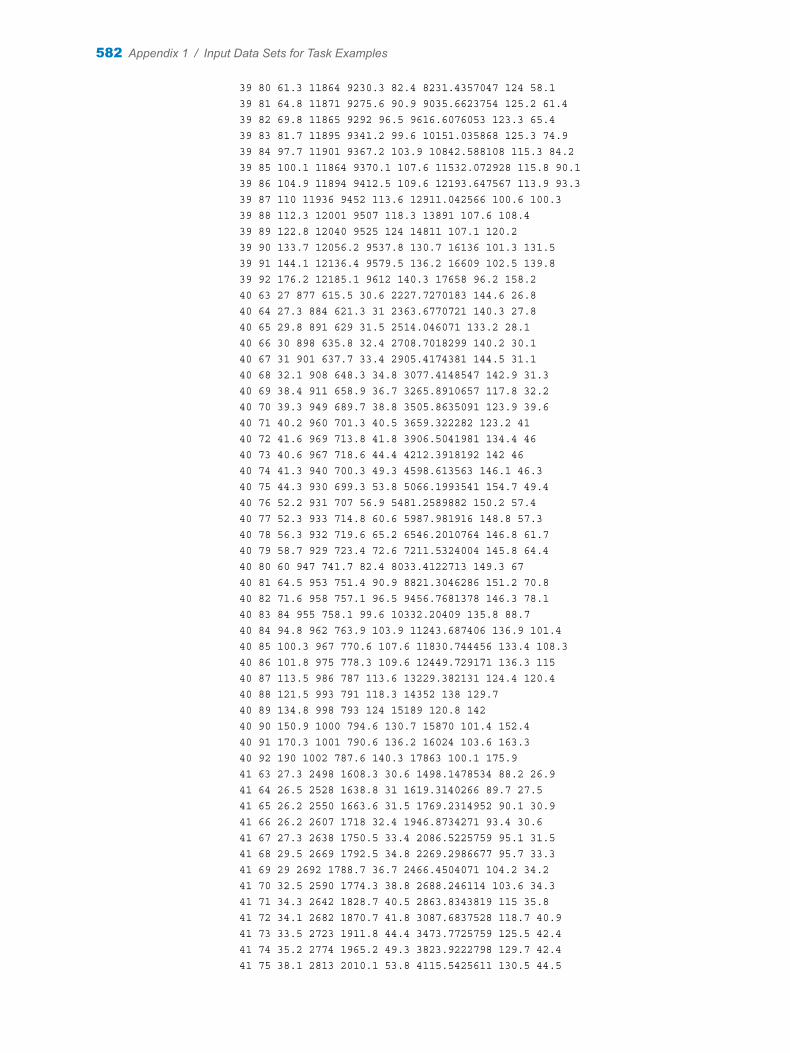
39 80 61.3 11864 9230.3 82.4 8231.4357047 124 58.1 39 81 64.8 11871 9275.6 90.9 9035.6623754 125.2 61.4 39 82 69.8 11865 9292 96.5 9616.6076053 123.3 65.4 39 83 81.7 11895 9341.2 99.6 10151.035868 125.3 74.9 39 84 97.7 11901 9367.2 103.9 10842.588108 115.3 84.2 39 85 100.1 11864 9370.1 107.6 11532.072928 115.8 90.1 39 86 104.9 11894 9412.5 109.6 12193.647567 113.9 93.3 39 87 110 11936 9452 113.6 12911.042566 100.6 100.3 39 88 112.3 12001 9507 118.3 13891 107.6 108.4 39 89 122.8 12040 9525 124 14811 107.1 120.2 39 90 133.7 12056.2 9537.8 130.7 16136 101.3 131.5 39 91 144.1 12136.4 9579.5 136.2 16609 102.5 139.8 39 92 176.2 12185.1 9612 140.3 17658 96.2 158.2 40 63 27 877 615.5 30.6 2227.7270183 144.6 26.8 40 64 27.3 884 621.3 31 2363.6770721 140.3 27.8 40 65 29.8 891 629 31.5 2514.046071 133.2 28.1 40 66 30 898 635.8 32.4 2708.7018299 140.2 30.1 40 67 31 901 637.7 33.4 2905.4174381 144.5 31.1 40 68 32.1 908 648.3 34.8 3077.4148547 142.9 31.3 40 69 38.4 911 658.9 36.7 3265.8910657 117.8 32.2 40 70 39.3 949 689.7 38.8 3505.8635091 123.9 39.6 40 71 40.2 960 701.3 40.5 3659.322282 123.2 41 40 72 41.6 969 713.8 41.8 3906.5041981 134.4 46 40 73 40.6 967 718.6 44.4 4212.3918192 142 46 40 74 41.3 940 700.3 49.3 4598.613563 146.1 46.3 40 75 44.3 930 699.3 53.8 5066.1993541 154.7 49.4 40 76 52.2 931 707 56.9 5481.2589882 150.2 57.4 40 77 52.3 933 714.8 60.6 5987.981916 148.8 57.3 40 78 56.3 932 719.6 65.2 6546.2010764 146.8 61.7 40 79 58.7 929 723.4 72.6 7211.5324004 145.8 64.4 40 80 60 947 741.7 82.4 8033.4122713 149.3 67 40 81 64.5 953 751.4 90.9 8821.3046286 151.2 70.8 40 82 71.6 958 757.1 96.5 9456.7681378 146.3 78.1 40 83 84 955 758.1 99.6 10332.20409 135.8 88.7 40 84 94.8 962 763.9 103.9 11243.687406 136.9 101.4 40 85 100.3 967 770.6 107.6 11830.744456 133.4 108.3 40 86 101.8 975 778.3 109.6 12449.729171 136.3 115 40 87 113.5 986 787 113.6 13229.382131 124.4 120.4 40 88 121.5 993 791 118.3 14352 138 129.7 40 89 134.8 998 793 124 15189 120.8 142 40 90 150.9 1000 794.6 130.7 15870 101.4 152.4 40 91 170.3 1001 790.6 136.2 16024 103.6 163.3 40 92 190 1002 787.6 140.3 17863 100.1 175.9 41 63 27.3 2498 1608.3 30.6 1498.1478534 88.2 26.9 41 64 26.5 2528 1638.8 31 1619.3140266 89.7 27.5 41 65 26.2 2550 1663.6 31.5 1769.2314952 90.1 30.9 41 66 26.2 2607 1718 32.4 1946.8734271 93.4 30.6 41 67 27.3 2638 1750.5 33.4 2086.5225759 95.1 31.5 41 68 29.5 2669 1792.5 34.8 2269.2986677 95.7 33.3 41 69 29 2692 1788.7 36.7 2466.4504071 104.2 34.2 41 70 32.5 2590 1774.3 38.8 2688.246114 103.6 34.3 41 71 34.3 2642 1828.7 40.5 2863.8343819 115 35.8 41 72 34.1 2682 1870.7 41.8 3087.6837528 118.7 40.9 41 73 33.5 2723 1911.8 44.4 3473.7725759 125.5 42.4 41 74 35.2 2774 1965.2 49.3 3823.9222798 129.7 42.4 41 75 38.1 2813 2010.1 53.8 4115.5425611 130.5 44.5
582 Appendix 1 / Input Data Sets for Task Examples
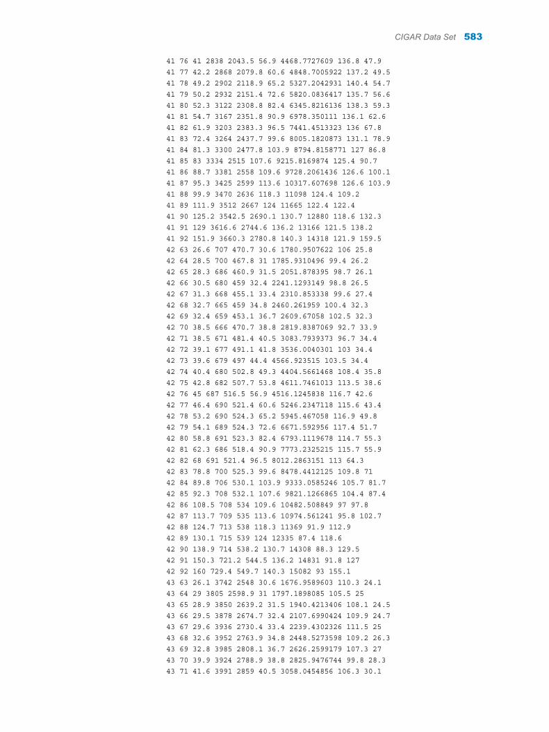
41 76 41 2838 2043.5 56.9 4468.7727609 136.8 47.9 41 77 42.2 2868 2079.8 60.6 4848.7005922 137.2 49.5 41 78 49.2 2902 2118.9 65.2 5327.2042931 140.4 54.7 41 79 50.2 2932 2151.4 72.6 5820.0836417 135.7 56.6 41 80 52.3 3122 2308.8 82.4 6345.8216136 138.3 59.3 41 81 54.7 3167 2351.8 90.9 6978.350111 136.1 62.6 41 82 61.9 3203 2383.3 96.5 7441.4513323 136 67.8 41 83 72.4 3264 2437.7 99.6 8005.1820873 131.1 78.9 41 84 81.3 3300 2477.8 103.9 8794.8158771 127 86.8 41 85 83 3334 2515 107.6 9215.8169874 125.4 90.7 41 86 88.7 3381 2558 109.6 9728.2061436 126.6 100.1 41 87 95.3 3425 2599 113.6 10317.607698 126.6 103.9 41 88 99.9 3470 2636 118.3 11098 124.4 109.2 41 89 111.9 3512 2667 124 11665 122.4 122.4 41 90 125.2 3542.5 2690.1 130.7 12880 118.6 132.3 41 91 129 3616.6 2744.6 136.2 13166 121.5 138.2 41 92 151.9 3660.3 2780.8 140.3 14318 121.9 159.5 42 63 26.6 707 470.7 30.6 1780.9507622 106 25.8 42 64 28.5 700 467.8 31 1785.9310496 99.4 26.2 42 65 28.3 686 460.9 31.5 2051.878395 98.7 26.1 42 66 30.5 680 459 32.4 2241.1293149 98.8 26.5 42 67 31.3 668 455.1 33.4 2310.853338 99.6 27.4 42 68 32.7 665 459 34.8 2460.261959 100.4 32.3 42 69 32.4 659 453.1 36.7 2609.67058 102.5 32.3 42 70 38.5 666 470.7 38.8 2819.8387069 92.7 33.9 42 71 38.5 671 481.4 40.5 3083.7939373 96.7 34.4 42 72 39.1 677 491.1 41.8 3536.0040301 103 34.4 42 73 39.6 679 497 44.4 4566.923515 103.5 34.4 42 74 40.4 680 502.8 49.3 4404.5661468 108.4 35.8 42 75 42.8 682 507.7 53.8 4611.7461013 113.5 38.6 42 76 45 687 516.5 56.9 4516.1245838 116.7 42.6 42 77 46.4 690 521.4 60.6 5246.2347118 115.6 43.4 42 78 53.2 690 524.3 65.2 5945.467058 116.9 49.8 42 79 54.1 689 524.3 72.6 6671.592956 117.4 51.7 42 80 58.8 691 523.3 82.4 6793.1119678 114.7 55.3 42 81 62.3 686 518.4 90.9 7773.2325215 115.7 55.9 42 82 68 691 521.4 96.5 8012.2863151 113 64.3 42 83 78.8 700 525.3 99.6 8478.4412125 109.8 71 42 84 89.8 706 530.1 103.9 9333.0585246 105.7 81.7 42 85 92.3 708 532.1 107.6 9821.1266865 104.4 87.4 42 86 108.5 708 534 109.6 10482.508849 97 97.8 42 87 113.7 709 535 113.6 10974.561241 95.8 102.7 42 88 124.7 713 538 118.3 11369 91.9 112.9 42 89 130.1 715 539 124 12335 87.4 118.6 42 90 138.9 714 538.2 130.7 14308 88.3 129.5 42 91 150.3 721.2 544.5 136.2 14831 91.8 127 42 92 160 729.4 549.7 140.3 15082 93 155.1 43 63 26.1 3742 2548 30.6 1676.9589603 110.3 24.1 43 64 29 3805 2598.9 31 1797.1898085 105.5 25 43 65 28.9 3850 2639.2 31.5 1940.4213406 108.1 24.5 43 66 29.5 3878 2674.7 32.4 2107.6990424 109.9 24.7 43 67 29.6 3936 2730.4 33.4 2239.4302326 111.5 25 43 68 32.6 3952 2763.9 34.8 2448.5273598 109.2 26.3 43 69 32.8 3985 2808.1 36.7 2626.2599179 107.3 27 43 70 39.9 3924 2788.9 38.8 2825.9476744 99.8 28.3 43 71 41.6 3991 2859 40.5 3058.0454856 106.3 30.1
CIGAR Data Set 583

43 72 41.6 4054 2923.3 41.8 3350.7814637 111.5 29.9 43 73 40.8 4089 2972.2 44.4 3753.2934337 109.7 30.1 43 74 42.5 4137 3030.7 49.3 4088.8943228 114.8 31.3 43 75 45.3 4180 3085.4 53.8 4397.3125855 117.4 33.3 43 76 48.3 4233 3147.8 56.9 4805.0519836 121.7 36 43 77 49.6 4289 3212.1 60.6 5222.2007524 124.6 36.9 43 78 54.8 4333 3261.1 65.2 5800.3543092 127.3 41.4 43 79 57.3 4380 3317.7 72.6 6399.4175787 127.2 43.4 43 80 60.3 4591 3476 82.4 6868.8406293 130.4 46.3 43 81 63.7 4612 3503.9 90.9 7577.6798906 129.1 49.4 43 82 68.3 4651 3545.1 96.5 8047.1029412 131.4 56.3 43 83 79.1 4685 3582.6 99.6 8501.8891929 129 66.4 43 84 88.3 4717 3621.9 103.9 9367.5512996 125.1 75.4 43 85 92.5 4766 3668.9 107.6 9810.8372093 128.7 79.3 43 86 98.8 4800 3709.3 109.6 10592.860465 129 85.4 43 87 103.5 4855 3763 113.6 11367.565321 130.6 90.5 43 88 112.1 4895 3798 118.3 12228 125.3 94.4 43 89 121.5 4940 3832 124 12854 124.7 103.8 43 90 135 4963.4 3850.2 130.7 13857 121.8 115.6 43 91 137.4 5040.8 3912 136.2 14328 120.6 120.5 43 92 163.9 5113 3967.7 140.3 15820 121 135.8 44 63 29.5 10257 6807.7 30.6 1896.9264812 113.4 27 44 64 29.7 10401 6910.9 31 2043.8787782 110.7 27.3 44 65 29.5 10591 7067.3 31.5 2179.4474465 120.5 27.2 44 66 33.8 10714 7190.8 32.4 2331.5741201 106.1 30 44 67 34.4 10858 7333.6 33.4 2530.2701836 109 30.4 44 68 34.9 11013 7495.8 34.8 2721.7221198 108.4 30.9 44 69 34.4 11187 7606.7 36.7 2928.6971859 111.3 30.9 44 70 40.4 11196 7817.1 38.8 3185.3462679 106.4 34.3 44 71 42 11445 8056.5 40.5 3350.9263209 108.9 38.8 44 72 46.9 11644 8261.1 41.8 3570.319891 108.6 39.8 44 73 46.4 11853 8474.4 44.4 4029.8045378 110.4 39.9 44 74 47.5 12049 8682.8 49.3 4427.1966648 114.7 41 44 75 50.6 12293 8926 53.8 4954.9830835 116 43.6 44 76 53.3 12571 9194.3 56.9 5447.5837409 121.4 46.4 44 77 53.3 12801 9419.2 60.6 5970.1957829 124.2 47.9 44 78 59.1 13047 9646 65.2 6739.1081536 126.6 53.1 44 79 62.2 13380 9924.9 72.6 7525.613405 126.4 55.5 44 80 63.7 14228 10564.7 82.4 8363.8624228 129.7 60 44 81 66.9 14766 10960.4 90.9 9404.9470055 129 62.6 44 82 73.8 15280 11331.9 96.5 9983.4423154 131.2 69.4 44 83 84.1 15724 11655.2 99.6 10367.381063 126.4 79.6 44 84 93.8 15989 11856.9 103.9 11138.363184 117.2 90.2 44 85 102.1 16389 12077 107.6 11755.148882 115.9 95.1 44 86 105.5 16689 12300.9 109.6 11910.380181 113.7 101.2 44 87 114.4 16789 12353 113.6 12184.622144 105.8 110.2 44 88 128 16841 12390 118.3 12908 96.5 113.7 44 89 137 16991 12545 124 13687 94.5 127.2 44 90 145.7 17173 12679.4 130.7 14590 85.6 133.6 44 91 173.6 17538.9 12913.8 136.2 15187 79.6 146.5 44 92 186 17849.3 13123.2 140.3 15965 77.2 165.4 45 63 24.9 973 592 30.6 2060.7057057 72 23.9 45 64 29.4 977 594.8 31 2181.1711712 62.3 24 45 65 29.7 994 609.9 31.5 2282.4474474 65 24.2 45 66 30.8 1010 624.9 32.4 2365.6006006 65.7 26.5 45 67 31.5 1022 637.1 33.4 2454.0840841 64.3 27.4
584 Appendix 1 / Input Data Sets for Task Examples
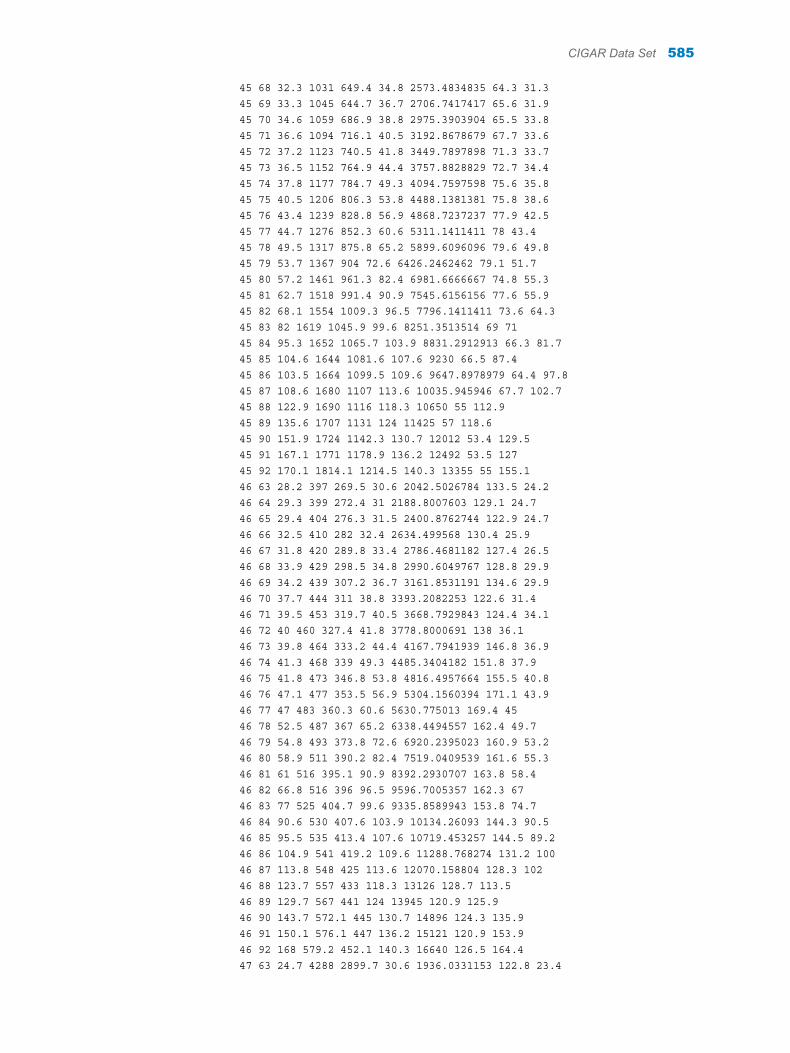
45 68 32.3 1031 649.4 34.8 2573.4834835 64.3 31.3 45 69 33.3 1045 644.7 36.7 2706.7417417 65.6 31.9 45 70 34.6 1059 686.9 38.8 2975.3903904 65.5 33.8 45 71 36.6 1094 716.1 40.5 3192.8678679 67.7 33.6 45 72 37.2 1123 740.5 41.8 3449.7897898 71.3 33.7 45 73 36.5 1152 764.9 44.4 3757.8828829 72.7 34.4 45 74 37.8 1177 784.7 49.3 4094.7597598 75.6 35.8 45 75 40.5 1206 806.3 53.8 4488.1381381 75.8 38.6 45 76 43.4 1239 828.8 56.9 4868.7237237 77.9 42.5 45 77 44.7 1276 852.3 60.6 5311.1411411 78 43.4 45 78 49.5 1317 875.8 65.2 5899.6096096 79.6 49.8 45 79 53.7 1367 904 72.6 6426.2462462 79.1 51.7 45 80 57.2 1461 961.3 82.4 6981.6666667 74.8 55.3 45 81 62.7 1518 991.4 90.9 7545.6156156 77.6 55.9 45 82 68.1 1554 1009.3 96.5 7796.1411411 73.6 64.3 45 83 82 1619 1045.9 99.6 8251.3513514 69 71 45 84 95.3 1652 1065.7 103.9 8831.2912913 66.3 81.7 45 85 104.6 1644 1081.6 107.6 9230 66.5 87.4 45 86 103.5 1664 1099.5 109.6 9647.8978979 64.4 97.8 45 87 108.6 1680 1107 113.6 10035.945946 67.7 102.7 45 88 122.9 1690 1116 118.3 10650 55 112.9 45 89 135.6 1707 1131 124 11425 57 118.6 45 90 151.9 1724 1142.3 130.7 12012 53.4 129.5 45 91 167.1 1771 1178.9 136.2 12492 53.5 127 45 92 170.1 1814.1 1214.5 140.3 13355 55 155.1 46 63 28.2 397 269.5 30.6 2042.5026784 133.5 24.2 46 64 29.3 399 272.4 31 2188.8007603 129.1 24.7 46 65 29.4 404 276.3 31.5 2400.8762744 122.9 24.7 46 66 32.5 410 282 32.4 2634.499568 130.4 25.9 46 67 31.8 420 289.8 33.4 2786.4681182 127.4 26.5 46 68 33.9 429 298.5 34.8 2990.6049767 128.8 29.9 46 69 34.2 439 307.2 36.7 3161.8531191 134.6 29.9 46 70 37.7 444 311 38.8 3393.2082253 122.6 31.4 46 71 39.5 453 319.7 40.5 3668.7929843 124.4 34.1 46 72 40 460 327.4 41.8 3778.8000691 138 36.1 46 73 39.8 464 333.2 44.4 4167.7941939 146.8 36.9 46 74 41.3 468 339 49.3 4485.3404182 151.8 37.9 46 75 41.8 473 346.8 53.8 4816.4957664 155.5 40.8 46 76 47.1 477 353.5 56.9 5304.1560394 171.1 43.9 46 77 47 483 360.3 60.6 5630.775013 169.4 45 46 78 52.5 487 367 65.2 6338.4494557 162.4 49.7 46 79 54.8 493 373.8 72.6 6920.2395023 160.9 53.2 46 80 58.9 511 390.2 82.4 7519.0409539 161.6 55.3 46 81 61 516 395.1 90.9 8392.2930707 163.8 58.4 46 82 66.8 516 396 96.5 9596.7005357 162.3 67 46 83 77 525 404.7 99.6 9335.8589943 153.8 74.7 46 84 90.6 530 407.6 103.9 10134.26093 144.3 90.5 46 85 95.5 535 413.4 107.6 10719.453257 144.5 89.2 46 86 104.9 541 419.2 109.6 11288.768274 131.2 100 46 87 113.8 548 425 113.6 12070.158804 128.3 102 46 88 123.7 557 433 118.3 13126 128.7 113.5 46 89 129.7 567 441 124 13945 120.9 125.9 46 90 143.7 572.1 445 130.7 14896 124.3 135.9 46 91 150.1 576.1 447 136.2 15121 120.9 153.9 46 92 168 579.2 452.1 140.3 16640 126.5 164.4 47 63 24.7 4288 2899.7 30.6 1936.0331153 122.8 23.4
CIGAR Data Set 585
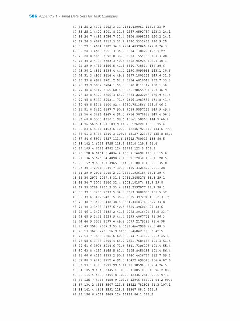
47 64 25.2 4371 2962.3 31 2134.439961 118.5 23.9 47 65 25.1 4420 3001.8 31.5 2267.0592737 123.3 24.1 47 66 24.7 4481 3056.7 32.4 2404.8998191 120.2 24.1 47 67 26.3 4541 3119.3 33.4 2580.3332406 120.9 25 47 68 27.1 4604 3182 34.8 2794.4037846 122.8 26.3 47 69 28.3 4669 3251.3 36.7 3024.138027 123.9 27 47 70 28.8 4648 3292.8 38.8 3284.1554195 124.3 28.3 47 71 30.2 4736 3383.3 40.5 3562.96925 128.4 30.1 47 72 29.9 4799 3456.5 41.8 3840.738834 137 30.6 47 73 30.1 4865 3538.4 44.4 4290.8090998 143.1 30.6 47 74 31.3 4924 3616.4 49.3 4677.1803256 149.6 31.5 47 75 33.6 4989 3701.2 53.8 5154.4010018 152.7 33.3 47 76 37.9 5052 3784.1 56.9 5570.0111312 158.1 36 47 77 38.4 5112 3865 60.6 6093.1786559 157.7 36.9 47 78 42.8 5177 3566.3 65.2 6684.2222068 155.9 41.4 47 79 45.8 5197 3993.1 72.6 7396.3983581 151.8 43.4 47 80 48.5 5346 4100 82.4 8230.7513566 148.9 46.3 47 81 51.8 5430 4187.7 90.9 9028.5557256 149.9 49.4 47 82 56.4 5491 4247.4 96.5 9754.3070822 147.4 56.3 47 83 68.8 5550 4310.1 99.6 10561.50967 144.7 66.4 47 84 76 5636 4391 103.9 11529.526228 136.8 75.4 47 85 83.6 5701 4453.6 107.6 12246.923612 134.6 79.3 47 86 91.3 5795 4540.3 109.6 13127.223459 135.8 85.4 47 87 94.6 5904 4627 113.6 13942.780019 133 90.5 47 88 102.1 6015 4725 118.3 15010 129.5 94.4 47 89 109.4 6098 4782 124 15936 122.5 103.8 47 90 128.6 6164.8 4834.4 130.7 16698 118.9 115.6 47 91 136.5 6263.4 4898.2 136.2 17038 109.1 120.5 47 92 157.9 6354.1 4965.1 140.3 18010 108.2 135.8 48 63 30.1 2961 2030.7 30.6 2409.3326822 99.1 28 48 64 29.9 2971 2045.2 31 2569.1936184 95.4 29.4 48 65 30 2973 2057.8 31.5 2764.3485276 98.3 29.1 48 66 34.7 3074 2140 32.4 3003.101874 86.9 29.8 48 67 35 3208 2250.3 33.4 3143.2397077 99.7 30.1 48 68 37.1 3296 2333.5 34.8 3363.3080096 101.5 32 48 69 37.6 3402 2421.5 36.7 3529.397294 100.2 31.9 48 70 38.7 3409 2438 38.8 3664.3448376 96.7 33.8 48 71 40.3 3433 2477.6 40.5 3829.396064 97 33.6 48 72 46.1 3423 2489.2 41.8 4072.3016424 88.5 33.7 48 73 45.9 3443 2528.9 44.4 4593.4067723 91 36.3 48 74 46.9 3503 2597.6 49.3 5079.2179292 98.6 38 48 75 49 3563 2667.3 53.8 5631.4647999 99.5 40.3 48 76 53 3623 2735 56.9 6166.0646842 100.3 42.5 48 77 53.7 3693 2806.6 60.6 6674.7131177 99.3 45.6 48 78 58.6 3793 2899.4 65.2 7521.7684683 101.3 51.5 48 79 61.6 3926 3014.6 72.6 8311.7306273 101.4 55.4 48 80 63.8 4132 3165.5 82.4 9105.8450185 101.4 56.4 48 81 66.6 4217 3233.2 90.9 9940.4436727 112.7 59.2 48 82 80.3 4245 3252.6 96.5 10492.690543 106.6 67.6 48 83 93.1 4300 3299 99.6 11018.985963 102.4 76.5 48 84 105.9 4349 3345.4 103.9 11805.833948 96.2 88.5 48 85 114.4 4406 3394.8 107.6 12336.2816 96.5 97.6 48 86 125.7 4463 3450.9 109.6 12946.659721 94.2 99.9 48 87 134.2 4538 3507 113.6 13522.781926 91.3 107.1 48 88 141.4 4648 3591 118.3 14347 88.2 121.9 48 89 150.6 4761 3669 124 15438 86.1 133.6
586 Appendix 1 / Input Data Sets for Task Examples
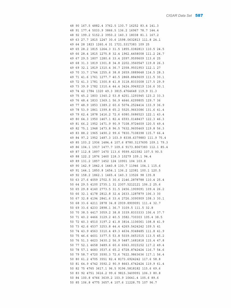
48 90 167.5 4882.4 3762.5 130.7 16252 83.4 141.3 48 91 177.4 5033.9 3866.5 136.2 16967 78.7 144.4 48 92 199.2 5152.2 3950.2 140.3 18038 81.1 167.2 49 63 27.7 1815 1247 30.6 1598.0632813 111.8 24.1 49 64 28 1823 1260.4 31 1721.5317383 109 25 49 65 28.2 1815 1264.3 31.5 1855.0382813 110.5 24.5 49 66 28.4 1815 1275.8 32.4 1962.4458008 111.2 24.7 49 67 29.5 1807 1280.6 33.4 2097.9599609 113.6 25 49 68 31.3 1819 1301.8 34.8 2202.3560547 119.8 26.3 49 69 32.1 1819 1310.4 36.7 2358.9501953 112.1 27 49 70 33.7 1744 1255.6 38.8 2659.0889648 114.5 28.3 49 71 41.6 1761 1277.7 40.5 2868.8849609 111.5 30.1 49 72 41.3 1781 1300.8 41.8 3118.8333008 117.5 29.9 49 73 39.9 1782 1310.4 44.4 3424.9949219 116.6 30.1 49 74 42 1784 1320 49.3 3815.4764648 119.9 31.3 49 75 45.2 1803 1340.2 53.8 4251.1293945 123.2 33.3 49 76 48.4 1833 1369.1 56.9 4646.6299805 129.7 36 49 77 48.9 1853 1389.2 60.6 5074.2524414 133.9 36.9 49 78 53.9 1861 1399.8 65.2 5525.9663086 131.6 41.4 49 79 62.4 1878 1416.2 72.6 6080.0686523 122.1 43.4 49 80 64.3 1950 1467.1 82.4 6593.0148437 122.3 46.3 49 81 66.2 1952 1471.9 90.9 7108.9724609 120.5 49.4 49 82 75.1 1948 1473.8 96.5 7632.9605469 119.8 56.3 49 83 88.2 1965 1490.2 99.6 7830.7108398 115.7 66.4 49 84 97.2 1952 1487.3 103.9 8338.6379883 111.9 75.4 49 85 103.2 1936 1484.4 107.6 8780.3137695 109.1 79.3 49 86 104.1 1917 1477.7 109.6 9173.8067383 112.1 85.4 49 87 112.8 1897 1470 113.6 9599.421582 107.5 90.5 49 88 122.2 1876 1460 118.3 10279 109.1 94.4 49 89 131.2 1857 1452 124 10901 104 103.8 49 90 142.9 1842.6 1440.8 130.7 11946 104.1 115.6 49 91 144.1 1850.8 1454.1 136.2 12381 100.1 120.5 49 92 158.2 1862.1 1465.4 140.3 13526 98 135.8 50 63 27.6 4059 2702.5 30.6 2146.2878788 110.4 25.4 50 64 29.5 4100 2735.1 31 2307.5212121 106.2 25.6 50 65 29.8 4140 2773.5 31.5 2456.1909091 109.4 26.2 50 66 32.1 4178 2812.8 32.4 2633.1287879 106.3 30 50 67 32.8 4194 2841.6 33.4 2726.3090909 108.3 30.1 50 68 33.6 4211 2878 34.8 2939.8909091 111.4 32.7 50 69 33.6 4233 2898.1 36.7 3109.5 111.5 32.8 50 70 38.5 4417 3059.2 38.8 3339.8333333 106.4 37.7 50 71 40.2 4466 3129.2 40.5 3582.730303 105.4 38.5 50 72 40.3 4510 3197.2 41.8 3814.1106061 108.8 41.9 50 73 42.6 4537 3253.8 44.4 4269.5424242 109.5 41 50 74 43.9 4563 3310.4 49.3 4634.9348485 111.8 41.9 50 75 46.6 4601 3377.5 53.8 5039.0651515 113.5 45.2 50 76 51.3 4623 3430.2 56.9 5487.1681818 115.4 47.8 50 77 52.1 4658 3489.6 60.6 6063.0015152 117.2 49.4 50 78 57.1 4683 3537.6 65.2 6728.8742424 116.7 54.6 50 79 58.7 4720 3590.3 72.6 7622.9863636 117.1 56.4 50 80 61.2 4705 3551 82.4 8173.6924242 117.6 58.8 50 81 64.9 4742 3592.2 90.9 8663.6742424 119.9 61.4 50 82 75 4765 3617.1 96.5 9196.5818182 115.6 69.6 50 83 92 4751 3616.2 99.6 9815.3409091 106.3 80.8 50 84 100.8 4766 3639.2 103.9 10641.4 105.6 89.6 50 85 106.8 4775 3657.4 107.6 11228.75 107 96.7
CIGAR Data Set 587
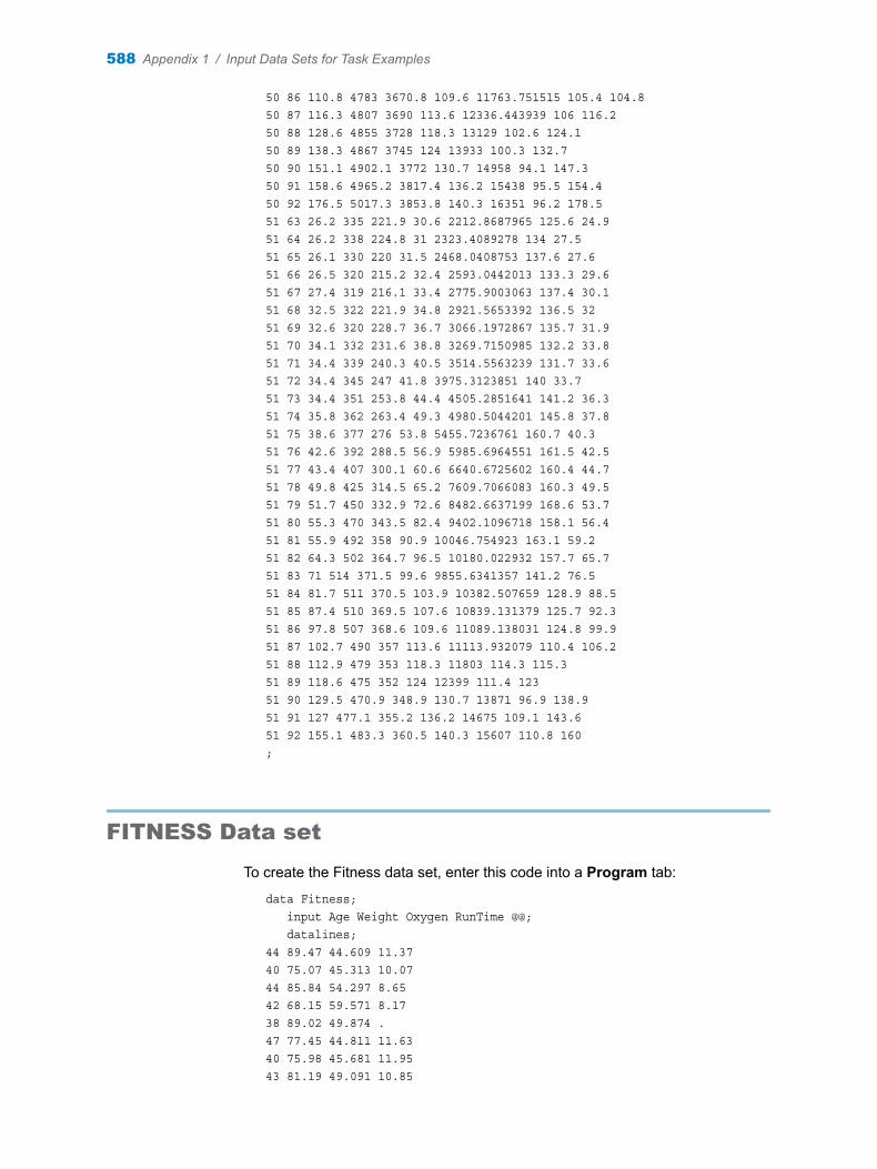
50 86 110.8 4783 3670.8 109.6 11763.751515 105.4 104.8 50 87 116.3 4807 3690 113.6 12336.443939 106 116.2 50 88 128.6 4855 3728 118.3 13129 102.6 124.1 50 89 138.3 4867 3745 124 13933 100.3 132.7 50 90 151.1 4902.1 3772 130.7 14958 94.1 147.3 50 91 158.6 4965.2 3817.4 136.2 15438 95.5 154.4 50 92 176.5 5017.3 3853.8 140.3 16351 96.2 178.5 51 63 26.2 335 221.9 30.6 2212.8687965 125.6 24.9 51 64 26.2 338 224.8 31 2323.4089278 134 27.5 51 65 26.1 330 220 31.5 2468.0408753 137.6 27.6 51 66 26.5 320 215.2 32.4 2593.0442013 133.3 29.6 51 67 27.4 319 216.1 33.4 2775.9003063 137.4 30.1 51 68 32.5 322 221.9 34.8 2921.5653392 136.5 32 51 69 32.6 320 228.7 36.7 3066.1972867 135.7 31.9 51 70 34.1 332 231.6 38.8 3269.7150985 132.2 33.8 51 71 34.4 339 240.3 40.5 3514.5563239 131.7 33.6 51 72 34.4 345 247 41.8 3975.3123851 140 33.7 51 73 34.4 351 253.8 44.4 4505.2851641 141.2 36.3 51 74 35.8 362 263.4 49.3 4980.5044201 145.8 37.8 51 75 38.6 377 276 53.8 5455.7236761 160.7 40.3 51 76 42.6 392 288.5 56.9 5985.6964551 161.5 42.5 51 77 43.4 407 300.1 60.6 6640.6725602 160.4 44.7 51 78 49.8 425 314.5 65.2 7609.7066083 160.3 49.5 51 79 51.7 450 332.9 72.6 8482.6637199 168.6 53.7 51 80 55.3 470 343.5 82.4 9402.1096718 158.1 56.4 51 81 55.9 492 358 90.9 10046.754923 163.1 59.2 51 82 64.3 502 364.7 96.5 10180.022932 157.7 65.7 51 83 71 514 371.5 99.6 9855.6341357 141.2 76.5 51 84 81.7 511 370.5 103.9 10382.507659 128.9 88.5 51 85 87.4 510 369.5 107.6 10839.131379 125.7 92.3 51 86 97.8 507 368.6 109.6 11089.138031 124.8 99.9 51 87 102.7 490 357 113.6 11113.932079 110.4 106.2 51 88 112.9 479 353 118.3 11803 114.3 115.3 51 89 118.6 475 352 124 12399 111.4 123 51 90 129.5 470.9 348.9 130.7 13871 96.9 138.9 51 91 127 477.1 355.2 136.2 14675 109.1 143.6 51 92 155.1 483.3 360.5 140.3 15607 110.8 160 ;
FITNESS Data set
To create the Fitness data set, enter this code into a Program tab:
data Fitness; input Age Weight Oxygen RunTime @@; datalines;44 89.47 44.609 11.3740 75.07 45.313 10.0744 85.84 54.297 8.6542 68.15 59.571 8.1738 89.02 49.874 .47 77.45 44.811 11.6340 75.98 45.681 11.9543 81.19 49.091 10.85
588 Appendix 1 / Input Data Sets for Task Examples
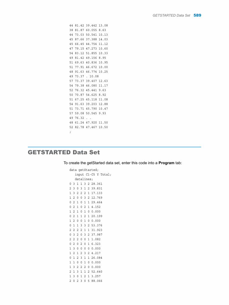
44 81.42 39.442 13.0838 81.87 60.055 8.6344 73.03 50.541 10.1345 87.66 37.388 14.0345 66.45 44.754 11.1247 79.15 47.273 10.6054 83.12 51.855 10.3349 81.42 49.156 8.9551 69.63 40.836 10.9551 77.91 46.672 10.0048 91.63 46.774 10.2549 73.37 . 10.0857 73.37 39.407 12.6354 79.38 46.080 11.1752 76.32 45.441 9.6350 70.87 54.625 8.9251 67.25 45.118 11.0854 91.63 39.203 12.8851 73.71 45.790 10.4757 59.08 50.545 9.9349 76.32 . .48 61.24 47.920 11.5052 82.78 47.467 10.50;
GETSTARTED Data Set
To create the getStarted data set, enter this code into a Program tab:
data getStarted; input C1-C5 Y Total; datalines;0 3 1 1 3 2 28.3612 3 0 3 1 2 39.8311 3 2 2 2 1 17.1331 2 0 0 3 2 12.7690 2 1 0 1 1 29.4640 2 1 0 2 1 4.1521 2 1 0 1 0 0.0000 2 1 1 2 1 20.1991 2 0 0 1 0 0.0000 1 1 3 3 2 53.3762 2 2 2 1 1 31.9230 3 2 0 3 2 37.9872 2 2 0 0 1 1.0820 2 0 2 0 1 6.3231 3 0 0 0 0 0.0001 2 1 2 3 2 4.2170 1 2 3 1 1 26.0841 1 0 0 1 0 0.0001 3 2 2 2 0 0.0002 1 3 1 1 2 52.6401 3 0 1 2 1 3.2572 0 2 3 0 5 88.066
GETSTARTED Data Set 589
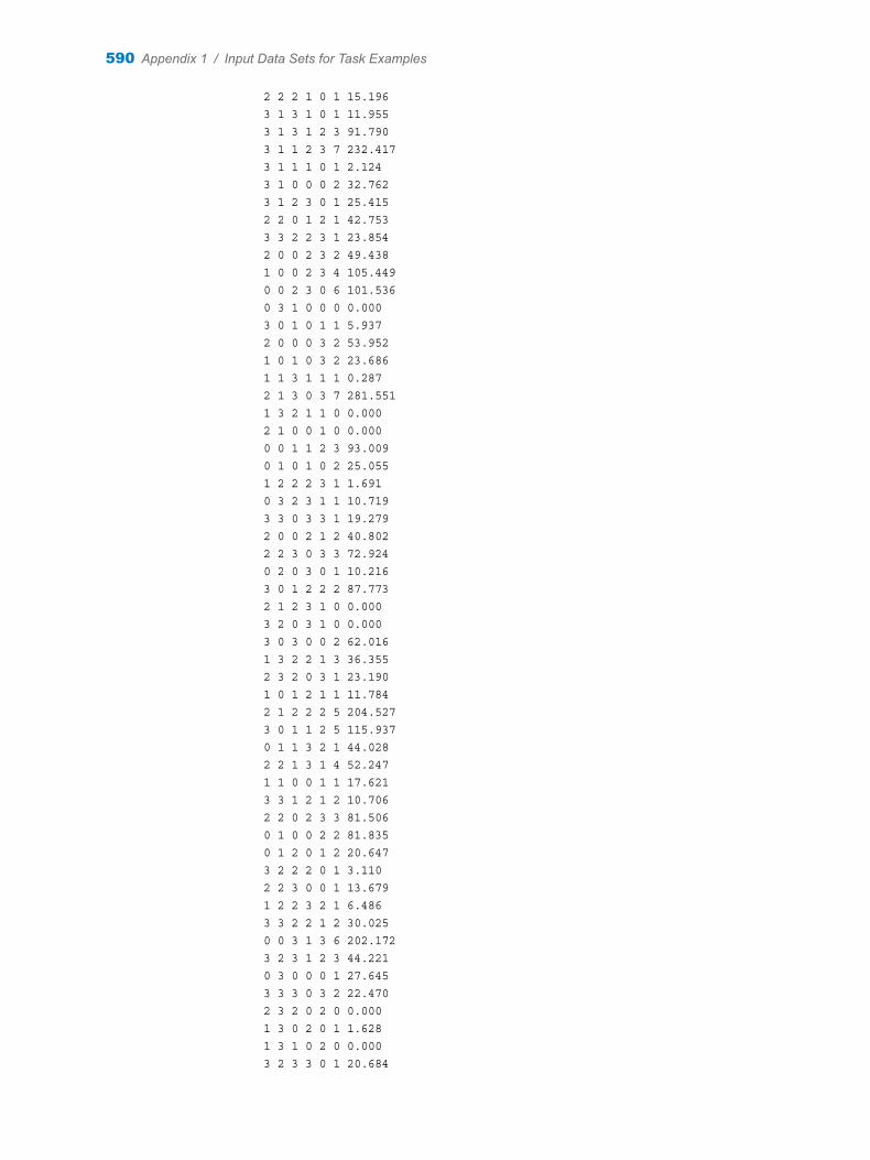
2 2 2 1 0 1 15.1963 1 3 1 0 1 11.9553 1 3 1 2 3 91.7903 1 1 2 3 7 232.4173 1 1 1 0 1 2.1243 1 0 0 0 2 32.7623 1 2 3 0 1 25.4152 2 0 1 2 1 42.7533 3 2 2 3 1 23.8542 0 0 2 3 2 49.4381 0 0 2 3 4 105.4490 0 2 3 0 6 101.5360 3 1 0 0 0 0.0003 0 1 0 1 1 5.9372 0 0 0 3 2 53.9521 0 1 0 3 2 23.6861 1 3 1 1 1 0.2872 1 3 0 3 7 281.5511 3 2 1 1 0 0.0002 1 0 0 1 0 0.0000 0 1 1 2 3 93.0090 1 0 1 0 2 25.0551 2 2 2 3 1 1.6910 3 2 3 1 1 10.7193 3 0 3 3 1 19.2792 0 0 2 1 2 40.8022 2 3 0 3 3 72.9240 2 0 3 0 1 10.2163 0 1 2 2 2 87.7732 1 2 3 1 0 0.0003 2 0 3 1 0 0.0003 0 3 0 0 2 62.0161 3 2 2 1 3 36.3552 3 2 0 3 1 23.1901 0 1 2 1 1 11.7842 1 2 2 2 5 204.5273 0 1 1 2 5 115.9370 1 1 3 2 1 44.0282 2 1 3 1 4 52.2471 1 0 0 1 1 17.6213 3 1 2 1 2 10.7062 2 0 2 3 3 81.5060 1 0 0 2 2 81.8350 1 2 0 1 2 20.6473 2 2 2 0 1 3.1102 2 3 0 0 1 13.6791 2 2 3 2 1 6.4863 3 2 2 1 2 30.0250 0 3 1 3 6 202.1723 2 3 1 2 3 44.2210 3 0 0 0 1 27.6453 3 3 0 3 2 22.4702 3 2 0 2 0 0.0001 3 0 2 0 1 1.6281 3 1 0 2 0 0.0003 2 3 3 0 1 20.684
590 Appendix 1 / Input Data Sets for Task Examples
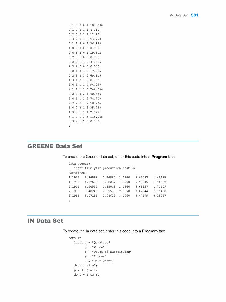
3 1 0 2 0 4 108.0000 1 2 2 1 1 4.6150 2 3 2 2 1 12.4610 3 2 0 1 3 53.7982 1 1 2 0 1 36.3201 0 3 0 0 0 0.0000 0 3 2 0 1 19.9020 2 3 1 0 0 0.0002 2 2 1 3 2 31.8153 3 3 0 0 0 0.0002 2 1 3 3 2 17.9150 2 3 2 3 2 69.3151 3 1 2 1 0 0.0003 0 1 1 1 4 94.0502 1 1 1 3 6 242.2660 2 0 3 2 1 40.8852 0 1 1 2 2 74.7082 2 2 2 3 2 50.7341 0 2 2 1 3 35.9501 3 3 1 1 1 2.7773 1 2 1 3 5 118.0650 3 2 1 2 0 0.000;
GREENE Data Set
To create the Greene data set, enter this code into a Program tab:
data greene; input firm year production cost @@;datalines;1 1955 5.36598 1.14867 1 1960 6.03787 1.451851 1965 6.37673 1.52257 1 1970 6.93245 1.766272 1955 6.54535 1.35041 2 1960 6.69827 1.711092 1965 7.40245 2.09519 2 1970 7.82644 2.394803 1955 8.07153 2.94628 3 1960 8.47679 3.25967;
IN Data Set
To create the In data set, enter this code into a Program tab:
data in; label q = "Quantity" p = "Price" s = "Price of Substitutes" y = "Income" u = "Unit Cost"; drop i e1 e2; p = 0; q = 0; do i = 1 to 60;
IN Data Set 591
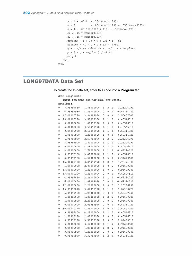
y = 1 + .05*i + .15*rannor(123); u = 2 + .05*rannor(123) + .05*rannor(123); s = 4 - .001*(i-10)*(i-110) + .5*rannor(123); e1 = .15 * rannor(123); e2 = .15 * rannor(123); demandx = 1 + .3 * y + .35 * s + e1; supplyx = -1 - 1 * u + e2 - .4*e1; q = 1.4/2.15 * demandx + .75/2.15 * supplyx; p = ( - q + supplyx ) / -1.4; output; end; run;
LONG97DATA Data Set
To create the In data set, enter this code into a Program tab:
data long97data; input fem ment phd mar kid5 art lnart; datalines; 0 7.99999860 1.38000000 1 2 3 1.25276290 0 6.99999950 4.29000000 0 0 0 -0.69314720 0 47.00000760 3.84999990 0 0 4 1.50407740 0 19.00000190 3.58999990 1 1 1 0.40546510 0 0.00000000 1.80999990 1 0 1 0.40546510 0 6.00000050 3.58999990 1 1 1 0.40546510 0 9.99999900 2.11999990 1 1 0 -0.69314720 0 1.99999990 4.29000000 1 0 0 -0.69314720 0 1.99999990 2.57999990 1 2 3 1.25276290 0 3.99999900 1.80000000 1 1 3 1.25276290 0 0.00000000 4.29000000 1 2 1 0.40546510 0 3.00000000 2.76000000 1 1 0 -0.69314720 0 9.99999900 3.41000010 1 1 1 0.40546510 0 6.99999950 4.34000020 1 3 2 0.91629080 0 15.00000100 3.84999990 1 2 5 1.70474800 0 1.99999990 2.09999990 1 0 2 0.91629080 0 13.00000000 4.29000000 1 0 2 0.91629080 0 15.00000100 4.29000000 0 0 1 0.40546510 0 4.99999810 2.26000000 1 1 0 -0.69314720 0 6.00000050 2.09999990 0 0 0 -0.69314720 0 12.00000000 2.26000000 1 0 3 1.25276290 0 15.99999810 3.84999990 1 1 6 1.87180220 0 6.99999950 4.29000000 0 0 4 1.50407740 0 6.00000050 1.80000000 1 2 2 0.91629080 0 1.99999990 2.26000000 0 0 2 0.91629080 0 0.00000000 2.09999990 0 0 0 -0.69314720 0 30.00000190 4.29000000 1 0 4 1.50407740 0 9.99999900 4.29000000 1 2 1 0.40546510 0 1.99999990 2.09999990 1 0 1 0.40546510 0 0.99999990 3.58999990 1 0 7 2.01490310 0 3.00000000 3.42000010 1 1 2 0.91629080 0 9.99999900 4.29000000 1 2 2 0.91629080 0 9.99999900 4.29000000 0 0 2 0.91629080 0 0.99999990 3.33999990 1 2 0 -0.69314720
592 Appendix 1 / Input Data Sets for Task Examples

0 1.99999990 4.29000000 0 0 0 -0.69314720 0 10.99999710 4.29000000 1 0 1 0.40546510 0 4.99999810 3.61999990 1 0 4 1.50407740 0 0.00000000 4.29000000 1 3 1 0.40546510 0 3.99999900 4.34000020 1 1 1 0.40546510 0 1.99999990 1.25000000 1 1 2 0.91629080 0 19.00000190 4.34000020 0 0 7 2.01490310 0 3.00000000 1.67000000 1 3 1 0.40546510 0 0.00000000 3.47000000 0 0 0 -0.69314720 0 0.99999990 2.26000000 1 1 1 0.40546510 0 0.99999990 1.80000000 1 0 1 0.40546510 0 17.00000000 4.34000020 1 2 2 0.91629080 0 3.00000000 3.58999990 0 0 2 0.91629080 0 0.99999990 1.75000000 1 2 1 0.40546510 0 6.00000050 4.29000000 0 0 1 0.40546510 0 0.00000000 2.09999990 1 1 0 -0.69314720 0 15.00000100 4.29000000 1 2 0 -0.69314720 0 0.00000000 2.09999990 1 1 0 -0.69314720 0 26.99999810 3.31999990 1 2 2 0.91629080 0 4.99999810 4.34000020 1 0 2 0.91629080 0 6.99999950 3.41000010 0 0 4 1.50407740 0 0.00000000 4.29000000 1 0 1 0.40546510 0 10.99999710 3.19000010 1 0 2 0.91629080 0 13.00000000 4.29000000 1 0 2 0.91629080 0 3.99999900 1.74000000 1 2 1 0.40546510 0 3.99999900 2.76000000 0 0 1 0.40546510 0 26.99999810 3.58999990 1 1 7 2.01490310 0 9.99999900 1.80999990 1 0 4 1.50407740 0 13.00000000 4.29000000 1 1 2 0.91629080 0 0.99999990 4.29000000 1 1 1 0.40546510 0 6.00000050 2.76000000 0 0 1 0.40546510 0 6.00000050 3.47000000 0 0 6 1.87180220 0 4.99999810 2.50000000 1 2 2 0.91629080 0 1.99999990 1.25000000 1 0 5 1.70474800 0 13.99999710 3.58999990 1 1 3 1.25276290 0 0.00000000 2.09999990 1 1 0 -0.69314720 0 12.00000000 3.58999990 1 0 1 0.40546510 0 6.99999950 3.58999990 1 3 0 -0.69314720 0 3.00000000 1.75000000 1 0 1 0.40546510 0 1.99999990 1.75000000 1 2 1 0.40546510 0 1.99999990 3.58999990 1 1 1 0.40546510 0 1.99999990 4.29000000 0 0 1 0.40546510 0 0.00000000 4.29000000 0 0 0 -0.69314720 0 0.00000000 2.09999990 1 1 0 -0.69314720 0 0.00000000 2.60999990 1 0 3 1.25276290 0 30.00000190 4.29000000 1 0 5 1.70474800 0 21.00000000 1.74000000 1 0 16 2.80336050 0 4.99999810 2.76000000 1 0 1 0.40546510 0 9.00000000 4.29000000 0 0 0 -0.69314720 0 7.99999860 2.76000000 1 2 1 0.40546510 0 25.00000000 4.29000000 1 2 3 1.25276290 0 0.00000000 3.47000000 1 1 5 1.70474800 0 4.99999810 2.57999990 1 2 0 -0.69314720 0 0.99999990 2.14000010 1 0 0 -0.69314720 0 4.99999810 2.26000000 0 0 0 -0.69314720 0 0.00000000 4.29000000 1 2 3 1.25276290
LONG97DATA Data Set 593
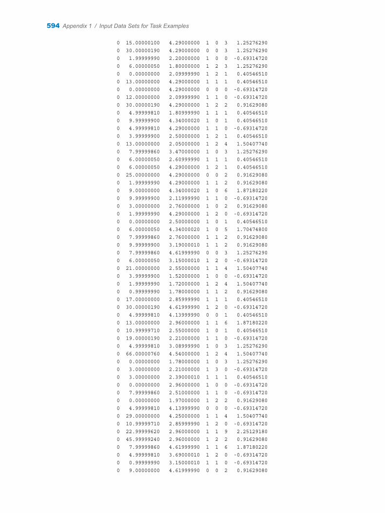
0 15.00000100 4.29000000 1 0 3 1.25276290 0 30.00000190 4.29000000 0 0 3 1.25276290 0 1.99999990 2.20000000 1 0 0 -0.69314720 0 6.00000050 1.80000000 1 2 3 1.25276290 0 0.00000000 2.09999990 1 2 1 0.40546510 0 13.00000000 4.29000000 1 1 1 0.40546510 0 0.00000000 4.29000000 0 0 0 -0.69314720 0 12.00000000 2.09999990 1 1 0 -0.69314720 0 30.00000190 4.29000000 1 2 2 0.91629080 0 4.99999810 1.80999990 1 1 1 0.40546510 0 9.99999900 4.34000020 1 0 1 0.40546510 0 4.99999810 4.29000000 1 1 0 -0.69314720 0 3.99999900 2.50000000 1 2 1 0.40546510 0 13.00000000 2.05000000 1 2 4 1.50407740 0 7.99999860 3.47000000 1 0 3 1.25276290 0 6.00000050 2.60999990 1 1 1 0.40546510 0 6.00000050 4.29000000 1 2 1 0.40546510 0 25.00000000 4.29000000 0 0 2 0.91629080 0 1.99999990 4.29000000 1 1 2 0.91629080 0 9.00000000 4.34000020 1 0 6 1.87180220 0 9.99999900 2.11999990 1 1 0 -0.69314720 0 3.00000000 2.76000000 1 0 2 0.91629080 0 1.99999990 4.29000000 1 2 0 -0.69314720 0 0.00000000 2.50000000 1 0 1 0.40546510 0 6.00000050 4.34000020 1 0 5 1.70474800 0 7.99999860 2.76000000 1 1 2 0.91629080 0 9.99999900 3.19000010 1 1 2 0.91629080 0 7.99999860 4.61999990 0 0 3 1.25276290 0 6.00000050 3.15000010 1 2 0 -0.69314720 0 21.00000000 2.55000000 1 1 4 1.50407740 0 3.99999900 1.52000000 1 0 0 -0.69314720 0 1.99999990 1.72000000 1 2 4 1.50407740 0 0.99999990 1.78000000 1 1 2 0.91629080 0 17.00000000 2.85999990 1 1 1 0.40546510 0 30.00000190 4.61999990 1 2 0 -0.69314720 0 4.99999810 4.13999990 0 0 1 0.40546510 0 13.00000000 2.96000000 1 1 6 1.87180220 0 10.99999710 2.55000000 1 0 1 0.40546510 0 19.00000190 2.21000000 1 1 0 -0.69314720 0 4.99999810 3.08999990 1 0 3 1.25276290 0 66.00000760 4.54000000 1 2 4 1.50407740 0 0.00000000 1.78000000 1 0 3 1.25276290 0 3.00000000 2.21000000 1 3 0 -0.69314720 0 3.00000000 2.39000010 1 1 1 0.40546510 0 0.00000000 2.96000000 1 0 0 -0.69314720 0 7.99999860 2.51000000 1 1 0 -0.69314720 0 0.00000000 1.97000000 1 2 2 0.91629080 0 4.99999810 4.13999990 0 0 0 -0.69314720 0 29.00000000 4.25000000 1 1 4 1.50407740 0 10.99999710 2.85999990 1 2 0 -0.69314720 0 22.99999620 2.96000000 1 1 9 2.25129180 0 45.99999240 2.96000000 1 2 2 0.91629080 0 7.99999860 4.61999990 1 1 6 1.87180220 0 4.99999810 3.69000010 1 2 0 -0.69314720 0 0.99999990 3.15000010 1 1 0 -0.69314720 0 9.00000000 4.61999990 0 0 2 0.91629080
594 Appendix 1 / Input Data Sets for Task Examples

0 1.99999990 3.35999990 1 0 0 -0.69314720 0 6.99999950 3.69000010 0 0 4 1.50407740 0 10.99999710 3.54000000 1 0 1 0.40546510 0 56.99999620 2.96000000 1 1 4 1.50407740 0 15.99999810 2.55999990 1 1 1 0.40546510 0 0.00000000 2.31999990 1 0 0 -0.69314720 0 3.00000000 2.31999990 1 0 0 -0.69314720 0 0.99999990 0.92000000 1 2 0 -0.69314720 0 9.99999900 4.54000000 1 0 0 -0.69314720 0 10.99999710 4.54000000 1 3 0 -0.69314720 0 10.99999710 1.76000000 1 1 5 1.70474800 0 15.99999810 2.55999990 0 0 1 0.40546510 0 4.99999810 2.39000010 1 1 0 -0.69314720 0 9.00000000 3.40000010 1 0 2 0.91629080 0 19.99999620 2.86999990 1 2 2 0.91629080 0 21.00000000 4.54000000 1 2 4 1.50407740 0 4.99999810 2.82999990 1 0 4 1.50407740 0 6.00000050 1.67999990 1 0 0 -0.69314720 0 12.00000000 3.54000000 0 0 3 1.25276290 0 0.00000000 1.76000000 1 0 2 0.91629080 0 10.99999710 3.15000010 1 3 1 0.40546510 0 3.00000000 2.51000000 1 0 0 -0.69314720 0 15.99999810 3.69000010 1 1 0 -0.69314720 0 10.99999710 1.76000000 1 1 4 1.50407740 0 4.99999810 1.86000000 1 1 12 2.52572870 0 0.99999990 2.76000000 1 3 0 -0.69314720 0 15.99999810 4.61999990 1 1 1 0.40546510 0 12.00000000 4.25000000 1 0 5 1.70474800 0 10.99999710 2.54000000 1 0 4 1.50407740 0 0.00000000 2.20000000 1 1 0 -0.69314720 0 0.00000000 1.76000000 1 0 2 0.91629080 0 3.00000000 2.85999990 1 3 3 1.25276290 0 13.00000000 3.40000010 1 2 0 -0.69314720 0 45.00000000 4.54000000 1 1 1 0.40546510 0 47.00000760 1.86000000 1 1 9 2.25129180 0 6.99999950 1.52000000 1 0 0 -0.69314720 0 6.99999950 2.55999990 1 1 2 0.91629080 0 19.00000190 2.21000000 1 0 0 -0.69314720 0 9.00000000 3.69000010 1 0 7 2.01490310 0 76.99998470 1.78000000 1 1 1 0.40546510 0 0.00000000 1.17999990 1 1 0 -0.69314720 0 3.99999900 2.00000000 1 0 1 0.40546510 0 19.00000190 2.21000000 1 0 0 -0.69314720 0 12.00000000 4.13999990 1 2 0 -0.69314720 0 0.99999990 2.85999990 1 3 0 -0.69314720 0 17.00000000 2.85999990 1 1 1 0.40546510 0 6.00000050 2.54000000 0 0 7 2.01490310 0 3.99999900 2.85999990 1 1 0 -0.69314720 0 6.00000050 2.52000000 0 0 4 1.50407740 0 3.00000000 1.52000000 1 1 2 0.91629080 0 4.99999810 3.08999990 1 1 3 1.25276290 0 3.00000000 1.17999990 1 1 0 -0.69314720 0 3.00000000 1.42000000 1 0 0 -0.69314720 0 15.00000100 4.61999990 0 0 7 2.01490310 0 0.00000000 2.96000000 1 2 1 0.40546510 0 9.99999900 4.54000000 0 0 2 0.91629080
LONG97DATA Data Set 595
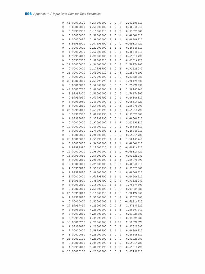
0 41.99999620 4.54000000 0 0 7 2.01490310 0 3.00000000 2.51000000 1 2 1 0.40546510 0 6.99999950 3.15000010 1 1 2 0.91629080 0 0.00000000 2.50000000 1 0 1 0.40546510 0 6.00000050 2.96000000 1 3 1 0.40546510 0 3.99999900 1.67999990 1 0 0 -0.69314720 0 0.00000000 1.22000000 1 1 1 0.40546510 0 1.99999990 1.52000000 1 0 1 0.40546510 0 4.99999810 2.21000000 1 1 0 -0.69314720 0 0.99999990 3.92000010 1 1 0 -0.69314720 0 13.00000000 4.54000000 1 0 5 1.70474800 0 0.00000000 1.17999990 1 0 2 0.91629080 0 26.00000000 3.69000010 1 0 3 1.25276290 0 0.99999990 1.72000000 1 0 2 0.91629080 0 25.00000000 2.57999990 1 1 5 1.70474800 0 3.00000000 1.52000000 0 0 3 1.25276290 0 47.00000760 1.86000000 1 1 4 1.50407740 0 3.99999900 2.50000000 1 0 5 1.70474800 0 0.99999990 4.61999990 1 0 1 0.40546510 0 6.99999950 1.40000000 1 2 0 -0.69314720 0 4.99999810 4.54000000 1 0 3 1.25276290 0 26.99999810 1.67999990 1 1 0 -0.69314720 0 0.99999990 2.82999990 1 0 2 0.91629080 0 4.99999810 3.35999990 0 0 1 0.40546510 0 0.00000000 1.97000000 1 1 7 2.01490310 0 12.00000000 3.40000010 0 0 1 0.40546510 0 3.99999900 1.74000000 1 1 1 0.40546510 0 0.00000000 2.96000000 0 0 0 -0.69314720 0 25.00000000 2.57999990 1 1 4 1.50407740 0 3.00000000 4.54000000 1 1 1 0.40546510 0 1.99999990 3.15000010 1 1 0 -0.69314720 0 12.00000000 2.96000000 1 2 0 -0.69314720 0 15.99999810 3.54000000 1 2 2 0.91629080 0 4.99999810 2.96000000 1 1 3 1.25276290 0 12.00000000 4.25000000 1 0 1 0.40546510 0 4.99999810 2.55999990 1 1 2 0.91629080 0 4.99999810 1.86000000 1 0 1 0.40546510 0 3.00000000 4.61999990 1 1 1 0.40546510 0 3.99999900 2.85999990 0 0 2 0.91629080 0 4.99999810 3.15000010 1 1 5 1.70474800 0 0.00000000 2.51000000 1 0 2 0.91629080 0 26.99999810 3.15000010 1 1 5 1.70474800 0 4.99999810 2.51000000 1 0 2 0.91629080 0 0.00000000 1.52000000 1 1 0 -0.69314720 0 17.99999810 4.29000000 0 0 6 1.87180220 0 4.99999810 4.29000000 1 1 4 1.50407740 0 7.99999860 4.29000000 1 2 2 0.91629080 0 3.99999900 2.09999990 1 0 2 0.91629080 0 35.00000760 4.29000000 1 1 12 2.52572870 0 4.99999810 4.29000000 0 0 2 0.91629080 0 9.00000000 3.58999990 1 1 1 0.40546510 0 6.00000050 4.29000000 1 0 1 0.40546510 0 24.00000190 4.29000000 1 0 2 0.91629080 0 0.00000000 2.09999990 1 1 0 -0.69314720 0 4.99999810 1.80999990 1 1 0 -0.69314720 0 19.00000190 4.29000000 0 0 7 2.01490310
596 Appendix 1 / Input Data Sets for Task Examples

0 3.00000000 4.29000000 0 0 1 0.40546510 0 1.99999990 4.29000000 1 1 1 0.40546510 0 3.99999900 1.25000000 1 0 3 1.25276290 0 9.99999900 3.58999990 1 0 1 0.40546510 0 7.99999860 2.09999990 1 1 1 0.40546510 0 1.99999990 4.29000000 1 0 4 1.50407740 0 19.00000190 4.29000000 1 1 3 1.25276290 0 0.99999990 3.47000000 1 1 1 0.40546510 0 3.00000000 3.19000010 1 0 1 0.40546510 0 4.99999810 3.19000010 1 2 1 0.40546510 0 0.00000000 2.09999990 1 0 1 0.40546510 0 21.00000000 3.58999990 1 1 5 1.70474800 0 13.99999710 4.29000000 1 1 1 0.40546510 0 0.00000000 2.09999990 1 0 0 -0.69314720 0 6.99999950 2.76000000 1 1 1 0.40546510 0 4.99999810 2.60999990 1 0 3 1.25276290 0 22.00000000 4.29000000 1 0 4 1.50407740 0 19.99999620 3.41000010 0 0 7 2.01490310 0 38.00000380 4.29000000 1 0 3 1.25276290 0 19.00000190 4.29000000 0 0 4 1.50407740 0 3.00000000 2.26000000 0 0 2 0.91629080 0 15.99999810 3.58999990 0 0 3 1.25276290 0 1.99999990 4.29000000 1 1 0 -0.69314720 0 3.00000000 2.05000000 0 0 1 0.40546510 0 12.00000000 4.29000000 1 2 1 0.40546510 0 35.00000760 4.29000000 0 0 0 -0.69314720 0 19.00000190 4.29000000 1 0 0 -0.69314720 0 1.99999990 4.29000000 0 0 0 -0.69314720 0 6.99999950 2.76000000 0 0 1 0.40546510 0 3.99999900 2.09999990 1 2 3 1.25276290 0 13.99999710 2.35999990 0 0 1 0.40546510 0 9.00000000 4.29000000 0 0 0 -0.69314720 0 7.99999860 3.58999990 0 0 0 -0.69314720 0 12.00000000 4.29000000 1 1 2 0.91629080 0 3.00000000 4.29000000 1 1 0 -0.69314720 0 0.99999990 4.29000000 1 0 1 0.40546510 0 9.99999900 4.29000000 0 0 1 0.40546510 0 21.00000000 3.41000010 0 0 4 1.50407740 0 13.00000000 4.29000000 1 1 0 -0.69314720 0 17.00000000 4.29000000 1 0 2 0.91629080 0 4.99999810 4.29000000 0 0 0 -0.69314720 0 1.99999990 2.14000010 0 0 0 -0.69314720 0 7.99999860 4.29000000 1 0 0 -0.69314720 0 1.99999990 2.50000000 1 1 2 0.91629080 0 4.99999810 2.60999990 1 1 3 1.25276290 0 0.99999990 1.80999990 1 2 0 -0.69314720 0 1.99999990 2.26000000 1 1 0 -0.69314720 0 3.99999900 3.61999990 1 2 1 0.40546510 0 9.00000000 4.29000000 1 2 1 0.40546510 0 9.00000000 4.29000000 0 0 0 -0.69314720 0 17.00000000 4.29000000 0 0 2 0.91629080 0 24.00000190 4.29000000 1 2 0 -0.69314720 0 3.99999900 3.47000000 1 0 4 1.50407740 0 13.99999710 4.29000000 1 1 2 0.91629080 0 4.99999810 3.58999990 1 1 1 0.40546510 0 9.99999900 1.80999990 0 0 1 0.40546510
LONG97DATA Data Set 597

0 17.99999810 4.29000000 1 1 3 1.25276290 0 0.99999990 4.29000000 1 1 0 -0.69314720 0 0.00000000 2.09999990 1 0 1 0.40546510 0 3.99999900 2.15000010 1 2 0 -0.69314720 0 7.99999860 4.29000000 1 0 0 -0.69314720 0 0.99999990 2.26000000 1 0 1 0.40546510 0 7.99999860 4.29000000 1 0 0 -0.69314720 0 13.00000000 4.29000000 1 2 0 -0.69314720 0 4.99999810 3.58999990 1 2 0 -0.69314720 0 6.99999950 3.41000010 1 2 0 -0.69314720 0 6.99999950 3.58999990 0 0 3 1.25276290 0 4.99999810 3.61999990 1 1 3 1.25276290 0 0.00000000 2.09999990 1 3 1 0.40546510 0 13.99999710 4.29000000 0 0 1 0.40546510 0 6.00000050 4.29000000 1 0 0 -0.69314720 0 4.99999810 2.26000000 1 1 1 0.40546510 0 7.99999860 2.76000000 1 0 3 1.25276290 0 3.99999900 2.60999990 1 1 1 0.40546510 0 9.00000000 4.29000000 0 0 2 0.91629080 0 3.00000000 2.09999990 1 1 2 0.91629080 0 1.99999990 3.47000000 1 1 0 -0.69314720 0 0.00000000 2.09999990 0 0 0 -0.69314720 0 10.99999710 4.29000000 0 0 1 0.40546510 0 9.00000000 4.29000000 0 0 1 0.40546510 0 7.99999860 2.96000000 1 0 1 0.40546510 0 1.99999990 2.96000000 1 0 2 0.91629080 0 17.99999810 4.61999990 1 0 3 1.25276290 0 3.00000000 1.42000000 1 0 3 1.25276290 0 1.99999990 4.54000000 1 0 1 0.40546510 0 6.99999950 2.52000000 1 0 0 -0.69314720 0 9.99999900 4.54000000 1 1 2 0.91629080 0 15.99999810 2.00000000 1 1 1 0.40546510 0 4.99999810 2.54000000 1 0 0 -0.69314720 0 0.00000000 2.50000000 1 0 2 0.91629080 0 7.99999860 4.54000000 0 0 0 -0.69314720 0 9.99999900 3.35999990 0 0 1 0.40546510 0 17.99999810 3.40000010 1 1 0 -0.69314720 0 12.00000000 1.67999990 1 1 1 0.40546510 0 9.00000000 2.00000000 0 0 1 0.40546510 0 39.00000000 2.85999990 1 0 1 0.40546510 0 17.99999810 4.61999990 1 0 1 0.40546510 0 15.00000100 4.13999990 1 0 1 0.40546510 0 15.99999810 4.13999990 1 0 2 0.91629080 0 1.99999990 2.96000000 0 0 0 -0.69314720 0 6.99999950 2.82999990 1 2 3 1.25276290 0 24.00000190 2.55000000 1 0 2 0.91629080 0 7.99999860 1.67999990 1 0 1 0.40546510 0 6.99999950 2.00000000 0 0 1 0.40546510 0 10.99999710 2.00000000 1 1 1 0.40546510 0 0.00000000 2.96000000 1 1 4 1.50407740 0 3.99999900 1.50500000 1 0 4 1.50407740 0 21.00000000 3.54000000 1 0 2 0.91629080 0 6.00000050 3.40000010 0 0 1 0.40546510 0 6.00000050 4.61999990 0 0 0 -0.69314720 0 7.99999860 2.82999990 0 0 3 1.25276290 0 3.99999900 2.54000000 1 0 1 0.40546510
598 Appendix 1 / Input Data Sets for Task Examples
0 12.00000000 2.86999990 0 0 1 0.40546510 0 15.00000100 1.86000000 0 0 1 0.40546510 0 0.00000000 3.92000010 1 1 1 0.40546510 0 4.99999810 3.69000010 1 1 1 0.40546510 0 15.00000100 2.85999990 1 2 4 1.50407740 0 4.99999810 4.54000000 0 0 0 -0.69314720 0 7.99999860 4.61999990 0 0 0 -0.69314720 0 13.00000000 2.85999990 1 1 0 -0.69314720 0 1.99999990 3.40000010 0 0 1 0.40546510 0 6.00000050 2.57999990 1 2 4 1.50407740 0 19.99999620 4.25000000 1 0 3 1.25276290 0 6.99999950 1.76000000 1 1 2 0.91629080 0 6.99999950 2.85999990 1 3 0 -0.69314720 0 15.99999810 3.69000010 1 2 4 1.50407740 0 13.00000000 3.40000010 1 0 0 -0.69314720 0 0.00000000 3.40000010 1 2 0 -0.69314720 0 0.99999990 4.54000000 1 2 0 -0.69314720 0 12.00000000 2.86999990 0 0 3 1.25276290 0 6.99999950 1.76000000 1 0 4 1.50407740 0 3.99999900 4.25000000 0 0 1 0.40546510 0 0.00000000 3.92000010 0 0 3 1.25276290 0 3.99999900 3.35999990 1 0 2 0.91629080 0 3.99999900 2.31999990 1 0 1 0.40546510 0 36.99999240 4.54000000 0 0 2 0.91629080 0 22.99999620 3.35999990 1 1 0 -0.69314720 0 7.99999860 2.00000000 1 3 2 0.91629080 0 7.99999860 3.92000010 1 1 1 0.40546510 0 1.99999990 3.92000010 0 0 1 0.40546510 0 0.00000000 3.35999990 0 0 1 0.40546510 0 0.99999990 1.78000000 1 0 1 0.40546510 0 21.00000000 3.54000000 1 1 1 0.40546510 0 9.99999900 3.92000010 0 0 2 0.91629080 0 7.99999860 2.31999990 0 0 3 1.25276290 0 33.99999240 1.67999990 1 0 1 0.40546510 0 13.99999710 3.08999990 0 0 2 0.91629080 0 6.00000050 2.57999990 1 1 0 -0.69314720 0 13.99999710 3.40000010 0 0 6 1.87180220 0 12.00000000 2.86999990 0 0 3 1.25276290 0 17.99999810 4.61999990 0 0 4 1.50407740 0 3.00000000 2.96000000 1 3 0 -0.69314720 0 6.00000050 1.86000000 1 2 2 0.91629080 0 1.99999990 1.22000000 1 1 0 -0.69314720 0 10.99999710 2.51000000 1 2 6 1.87180220 0 10.99999710 2.51000000 1 0 8 2.14006610 0 4.99999810 3.69000010 1 0 2 0.91629080 0 7.99999860 2.96000000 1 0 3 1.25276290 0 3.99999900 1.78000000 1 0 1 0.40546510 0 0.99999990 1.22000000 1 1 1 0.40546510 0 7.99999860 2.85999990 1 0 0 -0.69314720 0 19.00000190 3.69000010 0 0 7 2.01490310 0 1.99999990 2.11999990 0 0 0 -0.69314720 0 9.99999900 2.52000000 1 1 2 0.91629080 0 3.99999900 2.31999990 1 0 1 0.40546510 0 3.00000000 4.61999990 1 0 2 0.91629080 0 1.99999990 3.54000000 1 2 4 1.50407740 0 0.99999990 2.50000000 1 0 0 -0.69314720
LONG97DATA Data Set 599
0 4.99999810 1.67999990 0 0 0 -0.69314720 0 1.99999990 3.40000010 1 1 1 0.40546510 0 4.99999810 3.92000010 0 0 0 -0.69314720 0 52.99998090 4.54000000 1 1 5 1.70474800 0 54.99998860 4.54000000 0 0 2 0.91629080 0 0.00000000 2.50000000 0 0 0 -0.69314720 0 10.99999710 4.54000000 1 0 2 0.91629080 0 25.00000000 3.54000000 0 0 3 1.25276290 0 4.99999810 1.52000000 1 0 2 0.91629080 0 1.99999990 3.92000010 1 2 0 -0.69314720 0 7.99999860 4.61999990 1 0 2 0.91629080 0 0.00000000 3.92000010 1 0 3 1.25276290 0 4.99999810 2.31999990 1 2 0 -0.69314720 0 7.99999860 2.96000000 1 2 2 0.91629080 0 6.99999950 2.85999990 1 2 1 0.40546510 0 13.99999710 1.95000000 1 1 3 1.25276290 0 1.99999990 3.92000010 1 2 1 0.40546510 0 4.99999810 2.86999990 0 0 1 0.40546510 0 24.00000190 3.69000010 1 0 3 1.25276290 0 3.00000000 3.69000010 1 0 0 -0.69314720 0 3.99999900 2.39000010 0 0 2 0.91629080 0 3.00000000 1.95000000 1 2 3 1.25276290 0 10.99999710 3.35999990 0 0 5 1.70474800 0 3.99999900 2.39000010 1 1 2 0.91629080 0 26.00000000 3.69000010 0 0 2 0.91629080 0 3.99999900 2.96000000 1 1 5 1.70474800 0 1.99999990 3.21000000 1 0 0 -0.69314720 0 0.00000000 2.11999990 1 2 0 -0.69314720 0 52.99998090 4.54000000 1 1 2 0.91629080 0 3.99999900 2.31999990 1 0 3 1.25276290 0 6.00000050 2.54000000 1 1 3 1.25276290 0 1.99999990 2.85999990 1 1 1 0.40546510 0 13.99999710 3.47000000 1 0 3 1.25276290 0 15.00000100 2.86999990 0 0 4 1.50407740 0 3.99999900 2.31999990 1 0 0 -0.69314720 0 15.00000100 1.86000000 1 2 4 1.50407740 0 3.99999900 1.95000000 1 0 2 0.91629080 0 1.99999990 2.31999990 1 2 0 -0.69314720 0 19.99999620 4.25000000 1 2 1 0.40546510 0 3.99999900 1.97000000 0 0 6 1.87180220 0 41.99999620 1.86000000 1 0 19 2.97041440 0 7.99999860 3.69000010 1 1 0 -0.69314720 0 3.00000000 4.54000000 1 1 0 -0.69314720 0 9.00000000 3.54000000 1 0 4 1.50407740 0 9.99999900 4.54000000 1 1 1 0.40546510 0 6.99999950 2.85999990 1 2 11 2.44234700 0 25.00000000 3.35999990 1 0 0 -0.69314720 0 3.00000000 2.85999990 0 0 0 -0.69314720 0 3.99999900 2.96000000 1 2 0 -0.69314720 0 22.00000000 2.55999990 1 2 1 0.40546510 0 7.99999860 1.63000000 1 0 2 0.91629080 0 13.99999710 2.96000000 0 0 0 -0.69314720 0 0.00000000 2.96000000 1 0 1 0.40546510 0 7.99999860 1.63000000 1 1 1 0.40546510 0 0.00000000 2.96000000 0 0 0 -0.69314720 0 21.00000000 2.96000000 1 2 2 0.91629080
600 Appendix 1 / Input Data Sets for Task Examples
0 6.99999950 2.96000000 1 0 1 0.40546510 0 30.99998860 4.54000000 1 2 3 1.25276290 0 1.99999990 4.54000000 1 2 2 0.91629080 0 9.99999900 2.15000010 0 0 1 0.40546510 0 6.00000050 4.54000000 1 1 2 0.91629080 0 12.00000000 2.21000000 1 2 2 0.91629080 0 0.99999990 2.21000000 1 1 0 -0.69314720 0 29.00000000 4.54000000 0 0 2 0.91629080 0 9.99999900 2.21000000 1 1 3 1.25276290 0 6.00000050 2.21000000 1 0 0 -0.69314720 0 36.99999240 4.54000000 1 0 3 1.25276290 0 4.99999810 4.54000000 0 0 4 1.50407740 1 9.00000000 2.11999990 0 0 0 -0.69314720 1 1.99999990 2.11999990 1 0 0 -0.69314720 1 1.99999990 2.11999990 1 0 2 0.91629080 1 3.00000000 2.11999990 1 0 3 1.25276290 1 9.00000000 2.11999990 1 1 1 0.40546510 1 10.99999710 2.39000010 0 0 3 1.25276290 1 4.99999810 2.57999990 0 0 2 0.91629080 1 6.99999950 3.19000010 1 0 4 1.50407740 1 4.99999810 3.75000000 0 0 0 -0.69314720 1 3.00000000 3.58999990 0 0 1 0.40546510 1 1.99999990 2.57999990 0 0 2 0.91629080 1 0.00000000 3.75000000 0 0 3 1.25276290 1 4.99999810 3.75000000 1 0 0 -0.69314720 1 0.99999990 3.75000000 0 0 0 -0.69314720 1 3.99999900 1.22000000 1 2 2 0.91629080 1 13.99999710 3.75000000 0 0 0 -0.69314720 1 6.99999950 3.75000000 1 0 0 -0.69314720 1 26.00000000 3.75000000 0 0 0 -0.69314720 1 7.99999860 3.75000000 0 0 2 0.91629080 1 3.00000000 3.75000000 0 0 4 1.50407740 1 6.00000050 3.75000000 0 0 0 -0.69314720 1 21.00000000 3.75000000 0 0 1 0.40546510 1 7.99999860 3.75000000 1 0 2 0.91629080 1 3.99999900 3.75000000 0 0 0 -0.69314720 1 6.99999950 3.75000000 1 1 1 0.40546510 1 0.00000000 3.75000000 1 0 2 0.91629080 1 0.00000000 2.54000000 1 1 0 -0.69314720 1 0.99999990 2.54000000 1 0 0 -0.69314720 1 3.99999900 2.76000000 0 0 0 -0.69314720 1 1.99999990 4.13999990 0 0 0 -0.69314720 1 3.99999900 0.92000000 0 0 1 0.40546510 1 0.00000000 1.00500000 0 0 0 -0.69314720 1 6.00000050 3.08999990 0 0 2 0.91629080 1 3.00000000 3.08999990 1 1 2 0.91629080 1 0.00000000 1.79000000 0 0 0 -0.69314720 1 3.00000000 1.40000000 0 0 1 0.40546510 1 3.00000000 1.40000000 0 0 4 1.50407740 1 0.00000000 1.40000000 1 0 2 0.91629080 1 0.00000000 1.40000000 0 0 2 0.91629080 1 13.99999710 1.40000000 0 0 0 -0.69314720 1 12.00000000 1.40000000 0 0 1 0.40546510 1 1.99999990 1.40000000 0 0 1 0.40546510 1 6.00000050 2.00000000 0 0 1 0.40546510 1 10.99999710 4.34000020 1 0 2 0.91629080
LONG97DATA Data Set 601
1 6.00000050 4.34000020 1 0 4 1.50407740 1 0.00000000 1.75000000 0 0 0 -0.69314720 1 36.00000000 2.09999990 1 0 6 1.87180220 1 7.99999860 2.09999990 0 0 1 0.40546510 1 1.99999990 2.09999990 0 0 0 -0.69314720 1 10.99999710 3.58999990 1 0 2 0.91629080 1 10.99999710 3.58999990 1 2 2 0.91629080 1 17.99999810 3.58999990 0 0 0 -0.69314720 1 3.99999900 3.58999990 0 0 0 -0.69314720 1 17.99999810 3.58999990 1 0 10 2.35137530 1 7.99999860 3.58999990 0 0 1 0.40546510 1 19.00000190 3.41000010 1 0 3 1.25276290 1 3.99999900 3.41000010 1 0 4 1.50407740 1 4.99999810 3.41000010 1 2 0 -0.69314720 1 6.99999950 3.40000010 0 0 1 0.40546510 1 3.99999900 3.40000010 1 1 2 0.91629080 1 4.99999810 3.40000010 1 0 4 1.50407740 1 13.99999710 3.40000010 1 0 1 0.40546510 1 3.99999900 3.40000010 1 0 0 -0.69314720 1 3.99999900 2.52000000 0 0 3 1.25276290 1 0.00000000 2.52000000 0 0 1 0.40546510 1 15.00000100 3.69000010 1 1 2 0.91629080 1 0.99999990 3.69000010 1 0 1 0.40546510 1 3.00000000 3.69000010 1 1 0 -0.69314720 1 17.99999810 3.69000010 0 0 1 0.40546510 1 15.00000100 2.86999990 0 0 0 -0.69314720 1 4.99999810 2.86999990 1 0 1 0.40546510 1 17.99999810 2.86999990 1 0 1 0.40546510 1 9.00000000 2.86999990 0 0 2 0.91629080 1 6.00000050 2.86999990 0 0 4 1.50407740 1 15.00000100 2.86999990 1 0 1 0.40546510 1 3.99999900 3.35999990 0 0 2 0.91629080 1 1.99999990 3.35999990 1 2 0 -0.69314720 1 3.00000000 3.35999990 0 0 2 0.91629080 1 6.99999950 3.35999990 0 0 0 -0.69314720 1 15.99999810 4.54000000 1 0 4 1.50407740 1 48.00000000 4.54000000 1 2 2 0.91629080 1 15.00000100 4.54000000 1 0 5 1.70474800 1 36.99999240 4.54000000 0 0 1 0.40546510 1 9.99999900 4.54000000 1 0 2 0.91629080 1 13.00000000 4.54000000 0 0 2 0.91629080 1 6.00000050 4.54000000 1 2 0 -0.69314720 1 13.00000000 0.75500000 0 0 0 -0.69314720 1 6.99999950 4.54000000 1 1 2 0.91629080 1 9.00000000 4.54000000 1 0 2 0.91629080 1 4.99999810 4.54000000 0 0 2 0.91629080 1 15.00000100 4.54000000 0 0 6 1.87180220 1 3.00000000 4.54000000 0 0 3 1.25276290 1 13.99999710 4.54000000 0 0 0 -0.69314720 1 1.99999990 1.28000000 1 0 1 0.40546510 1 3.99999900 1.28000000 1 0 4 1.50407740 1 3.99999900 1.28000000 1 0 0 -0.69314720 1 0.00000000 2.50000000 1 1 0 -0.69314720 1 47.00000760 3.84999990 1 2 2 0.91629080 1 29.00000000 3.84999990 1 0 1 0.40546510 1 0.99999990 3.84999990 1 1 5 1.70474800
602 Appendix 1 / Input Data Sets for Task Examples
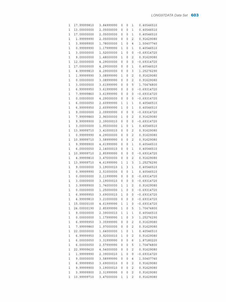
1 17.99999810 3.84999990 0 0 1 0.40546510 1 13.00000000 2.05000000 0 0 1 0.40546510 1 17.00000000 2.05000000 0 0 1 0.40546510 1 1.99999990 2.05000000 0 0 2 0.91629080 1 3.99999900 1.78000000 1 0 4 1.50407740 1 0.99999990 1.17999990 1 0 1 0.40546510 1 3.00000000 1.52000000 1 0 0 -0.69314720 1 9.00000000 1.48000000 1 0 2 0.91629080 1 12.00000000 4.29000000 0 0 0 -0.69314720 1 17.00000000 4.29000000 0 0 1 0.40546510 1 4.99999810 4.29000000 0 0 3 1.25276290 1 1.99999990 3.08999990 1 0 2 0.91629080 1 0.00000000 3.08999990 0 0 2 0.91629080 1 3.00000000 3.61999990 0 0 5 1.70474800 1 6.99999950 3.61999990 0 0 0 -0.69314720 1 7.99999860 3.61999990 0 0 0 -0.69314720 1 0.00000000 4.29000000 0 0 0 -0.69314720 1 6.00000050 2.60999990 1 1 1 0.40546510 1 6.99999950 2.60999990 1 0 1 0.40546510 1 9.00000000 2.09999990 0 0 0 -0.69314720 1 7.99999860 2.96000000 1 0 2 0.91629080 1 9.99999900 2.39000010 0 0 0 -0.69314720 1 3.00000000 1.95000000 1 0 1 0.40546510 1 13.99999710 3.41000010 0 0 2 0.91629080 1 0.99999990 4.29000000 0 0 2 0.91629080 1 10.99999710 3.58999990 0 0 2 0.91629080 1 9.99999900 4.61999990 0 0 1 0.40546510 1 6.00000050 2.14000010 0 0 1 0.40546510 1 10.99999710 2.85999990 0 0 0 -0.69314720 1 4.99999810 3.47000000 0 0 2 0.91629080 1 13.99999710 4.61999990 1 1 3 1.25276290 1 9.00000000 3.19000010 1 3 1 0.40546510 1 0.99999990 2.51000000 0 0 1 0.40546510 1 0.00000000 2.11999990 0 0 0 -0.69314720 1 3.00000000 3.19000010 0 0 0 -0.69314720 1 3.99999900 1.74000000 1 1 2 0.91629080 1 0.00000000 1.25000000 1 0 0 -0.69314720 1 6.99999950 3.69000010 1 0 0 -0.69314720 1 4.99999810 3.21000000 0 0 0 -0.69314720 1 15.00000100 4.61999990 1 1 0 -0.69314720 1 24.00000190 2.85999990 1 0 5 1.70474800 1 9.00000000 2.39000010 1 1 1 0.40546510 1 0.00000000 1.17999990 1 0 3 1.25276290 1 6.99999950 3.35999990 0 0 2 0.91629080 1 7.99999860 1.97000000 0 0 2 0.91629080 1 22.00000000 1.64000000 1 0 1 0.40546510 1 6.99999950 3.92000010 1 0 2 0.91629080 1 6.00000050 3.31999990 0 0 6 1.87180220 1 6.00000050 2.57999990 0 0 5 1.70474800 1 22.99999620 4.54000000 0 0 2 0.91629080 1 1.99999990 2.39000010 1 0 0 -0.69314720 1 9.00000000 3.58999990 0 0 4 1.50407740 1 6.99999950 3.69000010 0 0 2 0.91629080 1 9.99999900 3.19000010 0 0 2 0.91629080 1 3.99999900 2.31999990 0 0 2 0.91629080 1 10.99999710 3.47000000 1 1 2 0.91629080
LONG97DATA Data Set 603
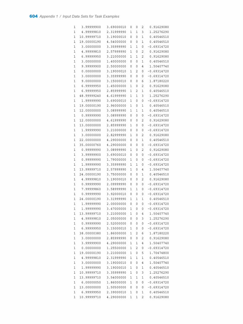
1 3.99999900 3.69000010 0 0 2 0.91629080 1 4.99999810 2.31999990 1 1 3 1.25276290 1 10.99999710 3.19000010 0 0 1 0.40546510 1 19.00000190 4.54000000 0 0 1 0.40546510 1 3.00000000 3.35999990 1 1 0 -0.69314720 1 4.99999810 2.57999990 1 0 2 0.91629080 1 6.99999950 3.21000000 1 1 2 0.91629080 1 3.00000000 1.40000000 0 0 1 0.40546510 1 9.99999900 2.50000000 0 0 4 1.50407740 1 0.00000000 3.19000010 1 2 0 -0.69314720 1 3.00000000 3.35999990 0 0 0 -0.69314720 1 9.00000000 3.15000010 0 0 6 1.87180220 1 6.99999950 1.45000000 1 0 2 0.91629080 1 6.99999950 2.85999990 1 2 1 0.40546510 1 48.99999240 4.61999990 1 1 3 1.25276290 1 1.99999990 3.69000010 1 0 0 -0.69314720 1 19.00000190 2.96000000 1 0 1 0.40546510 1 12.00000000 3.08999990 1 1 1 0.40546510 1 0.99999990 3.08999990 0 0 0 -0.69314720 1 12.00000000 4.61999990 0 0 2 0.91629080 1 13.00000000 2.85999990 1 0 0 -0.69314720 1 1.99999990 3.21000000 0 0 0 -0.69314720 1 3.00000000 2.82999990 1 0 2 0.91629080 1 22.00000000 4.29000000 0 0 1 0.40546510 1 35.00000760 4.29000000 0 0 0 -0.69314720 1 0.99999990 3.08999990 1 0 2 0.91629080 1 3.99999900 3.69000010 0 0 0 -0.69314720 1 0.99999990 1.79000000 1 0 0 -0.69314720 1 1.99999990 3.35999990 1 1 0 -0.69314720 1 13.99999710 2.57999990 1 0 4 1.50407740 1 24.00000190 3.75000000 0 0 1 0.40546510 1 4.99999810 3.19000010 0 0 2 0.91629080 1 0.99999990 2.09999990 0 0 0 -0.69314720 1 7.99999860 3.58999990 1 1 0 -0.69314720 1 0.99999990 3.92000010 0 0 0 -0.69314720 1 24.00000190 3.31999990 1 1 1 0.40546510 1 1.99999990 2.00000000 0 0 0 -0.69314720 1 1.99999990 3.47000000 1 0 0 -0.69314720 1 13.99999710 3.21000000 1 0 4 1.50407740 1 4.99999810 2.05000000 0 0 3 1.25276290 1 0.99999990 2.52000000 0 0 0 -0.69314720 1 6.99999950 3.15000010 1 0 0 -0.69314720 1 38.00000380 1.86000000 1 2 6 1.87180220 1 3.00000000 2.85999990 0 0 2 0.91629080 1 3.99999900 4.29000000 1 1 4 1.50407740 1 0.00000000 1.25500000 1 2 0 -0.69314720 1 19.00000190 3.21000000 1 0 5 1.70474800 1 4.99999810 2.31999990 1 1 1 0.40546510 1 3.00000000 3.19000010 0 0 4 1.50407740 1 1.99999990 3.19000010 1 0 1 0.40546510 1 10.99999710 3.35999990 1 0 3 1.25276290 1 13.99999710 3.54000000 1 1 1 0.40546510 1 6.00000050 1.86000000 1 0 0 -0.69314720 1 13.00000000 1.50500000 0 0 0 -0.69314720 1 6.99999950 2.39000010 1 0 1 0.40546510 1 10.99999710 4.29000000 1 1 2 0.91629080
604 Appendix 1 / Input Data Sets for Task Examples

1 9.00000000 2.00000000 1 1 0 -0.69314720 1 3.99999900 3.92000010 0 0 1 0.40546510 1 6.00000050 4.29000000 1 0 2 0.91629080 1 6.00000050 3.35999990 0 0 1 0.40546510 1 13.99999710 4.61999990 1 0 3 1.25276290 1 6.00000050 2.00000000 0 0 1 0.40546510 1 4.99999810 3.58999990 1 0 2 0.91629080 1 6.00000050 2.86999990 0 0 1 0.40546510 1 3.99999900 2.96000000 0 0 0 -0.69314720 1 10.99999710 3.47000000 1 0 0 -0.69314720 1 7.99999860 3.19000010 1 0 4 1.50407740 1 3.00000000 2.85999990 1 1 0 -0.69314720 1 15.99999810 2.52000000 1 0 2 0.91629080 1 6.00000050 4.29000000 0 0 1 0.40546510 1 0.00000000 1.25500000 0 0 1 0.40546510 1 1.99999990 1.83000000 1 0 0 -0.69314720 1 12.00000000 4.29000000 0 0 3 1.25276290 1 7.99999860 2.96000000 1 0 0 -0.69314720 1 0.99999990 2.31999990 1 0 1 0.40546510 1 10.99999710 1.22000000 1 1 0 -0.69314720 1 10.99999710 4.29000000 1 0 1 0.40546510 1 1.99999990 4.25000000 0 0 1 0.40546510 1 36.00000000 2.55000000 0 0 2 0.91629080 1 10.99999710 1.95000000 1 0 1 0.40546510 1 1.99999990 3.69000010 0 0 0 -0.69314720 1 25.00000000 4.29000000 0 0 1 0.40546510 1 4.99999810 3.19000010 1 0 2 0.91629080 1 12.00000000 3.54000000 1 1 4 1.50407740 1 4.99999810 3.54000000 1 0 4 1.50407740 1 7.99999860 3.54000000 1 1 0 -0.69314720 1 0.99999990 1.86000000 1 1 3 1.25276290 1 3.00000000 4.61999990 0 0 4 1.50407740 1 15.99999810 4.61999990 1 0 1 0.40546510 1 9.99999900 4.61999990 1 0 3 1.25276290 1 13.00000000 4.54000000 1 0 1 0.40546510 1 0.99999990 3.47000000 1 0 0 -0.69314720 1 15.99999810 2.85999990 0 0 0 -0.69314720 1 6.99999950 2.00000000 1 0 0 -0.69314720 1 1.99999990 2.00000000 0 0 0 -0.69314720 1 3.00000000 2.60999990 1 0 0 -0.69314720 1 6.00000050 2.05000000 0 0 0 -0.69314720 1 6.00000050 2.05000000 0 0 0 -0.69314720 1 4.99999810 3.54000000 0 0 0 -0.69314720 1 0.00000000 0.92000000 1 0 2 0.91629080 1 0.00000000 1.79000000 1 0 0 -0.69314720 1 6.00000050 2.00000000 1 0 0 -0.69314720 1 7.99999860 3.15000010 0 0 4 1.50407740 1 15.99999810 2.26000000 1 0 5 1.70474800 1 3.99999900 2.26000000 0 0 1 0.40546510 1 0.99999990 4.29000000 1 0 6 1.87180220 1 21.00000000 4.29000000 1 0 1 0.40546510 1 9.00000000 4.54000000 0 0 1 0.40546510 1 3.00000000 3.35999990 1 1 0 -0.69314720 1 1.99999990 2.52000000 0 0 0 -0.69314720 1 9.99999900 4.29000000 0 0 3 1.25276290 1 9.00000000 4.29000000 0 0 0 -0.69314720
LONG97DATA Data Set 605

1 12.00000000 4.54000000 0 0 2 0.91629080 1 0.00000000 2.50000000 0 0 0 -0.69314720 1 1.99999990 2.76000000 0 0 1 0.40546510 1 0.00000000 2.55000000 1 1 0 -0.69314720 1 0.00000000 4.61999990 1 0 0 -0.69314720 1 6.00000050 1.63000000 0 0 2 0.91629080 1 3.00000000 3.47000000 1 0 1 0.40546510 1 30.99998860 3.41000010 1 0 2 0.91629080 1 0.99999990 4.29000000 0 0 0 -0.69314720 1 6.99999950 2.96000000 1 0 0 -0.69314720 1 0.00000000 4.61999990 1 0 5 1.70474800 1 12.00000000 3.58999990 1 0 0 -0.69314720 1 12.00000000 3.69000010 1 0 3 1.25276290 1 1.99999990 4.54000000 1 0 1 0.40546510 1 10.99999710 3.33999990 0 0 4 1.50407740 1 1.99999990 2.51000000 1 1 4 1.50407740 1 3.99999900 3.15000010 1 0 3 1.25276290 1 3.00000000 3.19000010 1 0 1 0.40546510 1 17.99999810 3.19000010 0 0 1 0.40546510 1 1.99999990 3.84999990 0 0 1 0.40546510 1 3.99999900 3.33999990 1 1 2 0.91629080 1 15.00000100 4.29000000 0 0 2 0.91629080 1 3.99999900 4.29000000 0 0 2 0.91629080 1 21.00000000 4.29000000 0 0 2 0.91629080 1 3.99999900 4.29000000 1 1 0 -0.69314720 1 0.00000000 2.96000000 1 0 0 -0.69314720 1 0.99999990 1.78000000 1 0 0 -0.69314720 1 17.00000000 3.54000000 1 2 1 0.40546510 1 3.00000000 3.69000010 1 0 0 -0.69314720 1 1.99999990 3.35999990 0 0 3 1.25276290 1 1.99999990 3.54000000 1 0 0 -0.69314720 1 0.99999990 3.54000000 1 1 0 -0.69314720 1 3.00000000 1.22000000 1 1 3 1.25276290 1 3.99999900 3.35999990 0 0 1 0.40546510 1 1.99999990 2.21000000 0 0 1 0.40546510 1 3.99999900 2.25000000 0 0 1 0.40546510 1 17.00000000 4.61999990 1 1 2 0.91629080 1 4.99999810 3.58999990 1 0 1 0.40546510 1 0.99999990 4.29000000 1 0 0 -0.69314720 1 1.99999990 2.11999990 0 0 2 0.91629080 1 3.00000000 2.26000000 0 0 2 0.91629080 1 3.00000000 2.26000000 1 0 4 1.50407740 1 4.99999810 4.29000000 0 0 0 -0.69314720 1 3.00000000 3.58999990 1 1 3 1.25276290 1 13.00000000 4.29000000 1 2 1 0.40546510 1 1.99999990 2.00000000 0 0 1 0.40546510 1 0.00000000 1.97000000 1 2 0 -0.69314720 1 7.99999860 3.92000010 1 0 0 -0.69314720 1 39.00000000 2.85999990 0 0 4 1.50407740 1 26.00000000 2.82999990 0 0 2 0.91629080 1 3.00000000 3.35999990 1 1 3 1.25276290 1 22.99999620 2.55999990 0 0 4 1.50407740 1 7.99999860 1.63000000 0 0 1 0.40546510 1 22.00000000 4.61999990 0 0 3 1.25276290 1 4.99999810 4.61999990 0 0 1 0.40546510 1 21.00000000 4.29000000 1 0 3 1.25276290
606 Appendix 1 / Input Data Sets for Task Examples

1 6.00000050 4.29000000 1 1 0 -0.69314720 1 3.99999900 4.29000000 1 1 2 0.91629080 1 24.00000190 4.29000000 1 0 6 1.87180220 1 6.00000050 4.29000000 1 0 1 0.40546510 1 33.99999240 3.35999990 0 0 1 0.40546510 1 0.00000000 3.21000000 0 0 2 0.91629080 1 9.99999900 2.00000000 0 0 1 0.40546510 1 1.99999990 3.21000000 1 2 2 0.91629080 1 3.00000000 2.57999990 1 2 2 0.91629080 1 3.00000000 2.57999990 1 0 0 -0.69314720 1 0.99999990 2.82999990 0 0 0 -0.69314720 1 6.00000050 3.19000010 0 0 1 0.40546510 1 3.00000000 3.47000000 0 0 1 0.40546510 1 22.99999620 4.61999990 1 0 2 0.91629080 1 13.00000000 4.25000000 1 0 4 1.50407740 1 4.99999810 1.86000000 1 0 2 0.91629080 1 9.00000000 4.29000000 1 1 0 -0.69314720 1 9.00000000 3.35999990 0 0 0 -0.69314720 1 9.99999900 1.80000000 1 0 2 0.91629080 1 0.00000000 1.65500000 0 0 1 0.40546510 1 6.00000050 2.85999990 0 0 0 -0.69314720 1 13.99999710 4.61999990 0 0 2 0.91629080 1 3.00000000 4.29000000 0 0 0 -0.69314720 1 4.99999810 2.35999990 1 0 4 1.50407740 1 10.99999710 1.80999990 1 0 1 0.40546510 1 32.00001140 3.58999990 1 0 1 0.40546510 1 9.99999900 1.76000000 0 0 0 -0.69314720 1 4.99999810 2.00000000 1 0 1 0.40546510 1 13.99999710 3.58999990 0 0 5 1.70474800 1 6.00000050 2.26000000 1 0 3 1.25276290 1 3.99999900 2.26000000 0 0 1 0.40546510 1 3.99999900 1.76000000 1 1 1 0.40546510 1 0.99999990 3.58999990 1 0 1 0.40546510 1 0.99999990 3.58999990 1 0 0 -0.69314720 1 4.99999810 2.82999990 1 1 1 0.40546510 1 1.99999990 2.57999990 0 0 1 0.40546510 1 17.99999810 4.61999990 1 0 1 0.40546510 1 15.00000100 2.31999990 0 0 1 0.40546510 1 0.00000000 2.39000010 1 0 0 -0.69314720 1 22.00000000 2.96000000 1 0 3 1.25276290 1 10.99999710 2.11999990 0 0 0 -0.69314720 1 17.99999810 4.61999990 1 0 1 0.40546510 1 3.00000000 2.25000000 1 0 1 0.40546510 1 7.99999860 1.76000000 1 0 1 0.40546510 1 12.00000000 4.54000000 0 0 6 1.87180220 1 9.99999900 3.69000010 1 1 2 0.91629080 1 1.99999990 1.25000000 0 0 0 -0.69314720 1 4.99999810 1.25000000 1 0 1 0.40546510 1 3.99999900 3.19000010 1 0 0 -0.69314720 1 0.00000000 2.57999990 1 2 0 -0.69314720 1 6.99999950 2.00000000 1 1 2 0.91629080 1 0.99999990 2.76000000 0 0 0 -0.69314720 1 3.99999900 2.54000000 0 0 2 0.91629080 1 0.00000000 3.19000010 0 0 0 -0.69314720 1 9.00000000 3.08999990 1 2 1 0.40546510 1 3.99999900 3.19000010 0 0 2 0.91629080
LONG97DATA Data Set 607
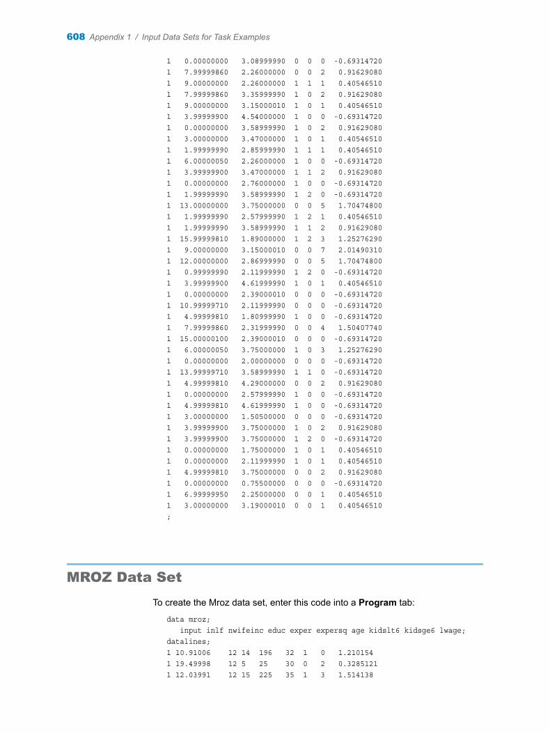
1 0.00000000 3.08999990 0 0 0 -0.69314720 1 7.99999860 2.26000000 0 0 2 0.91629080 1 9.00000000 2.26000000 1 1 1 0.40546510 1 7.99999860 3.35999990 1 0 2 0.91629080 1 9.00000000 3.15000010 1 0 1 0.40546510 1 3.99999900 4.54000000 1 0 0 -0.69314720 1 0.00000000 3.58999990 1 0 2 0.91629080 1 3.00000000 3.47000000 1 0 1 0.40546510 1 1.99999990 2.85999990 1 1 1 0.40546510 1 6.00000050 2.26000000 1 0 0 -0.69314720 1 3.99999900 3.47000000 1 1 2 0.91629080 1 0.00000000 2.76000000 1 0 0 -0.69314720 1 1.99999990 3.58999990 1 2 0 -0.69314720 1 13.00000000 3.75000000 0 0 5 1.70474800 1 1.99999990 2.57999990 1 2 1 0.40546510 1 1.99999990 3.58999990 1 1 2 0.91629080 1 15.99999810 1.89000000 1 2 3 1.25276290 1 9.00000000 3.15000010 0 0 7 2.01490310 1 12.00000000 2.86999990 0 0 5 1.70474800 1 0.99999990 2.11999990 1 2 0 -0.69314720 1 3.99999900 4.61999990 1 0 1 0.40546510 1 0.00000000 2.39000010 0 0 0 -0.69314720 1 10.99999710 2.11999990 0 0 0 -0.69314720 1 4.99999810 1.80999990 1 0 0 -0.69314720 1 7.99999860 2.31999990 0 0 4 1.50407740 1 15.00000100 2.39000010 0 0 0 -0.69314720 1 6.00000050 3.75000000 1 0 3 1.25276290 1 0.00000000 2.00000000 0 0 0 -0.69314720 1 13.99999710 3.58999990 1 1 0 -0.69314720 1 4.99999810 4.29000000 0 0 2 0.91629080 1 0.00000000 2.57999990 1 0 0 -0.69314720 1 4.99999810 4.61999990 1 0 0 -0.69314720 1 3.00000000 1.50500000 0 0 0 -0.69314720 1 3.99999900 3.75000000 1 0 2 0.91629080 1 3.99999900 3.75000000 1 2 0 -0.69314720 1 0.00000000 1.75000000 1 0 1 0.40546510 1 0.00000000 2.11999990 1 0 1 0.40546510 1 4.99999810 3.75000000 0 0 2 0.91629080 1 0.00000000 0.75500000 0 0 0 -0.69314720 1 6.99999950 2.25000000 0 0 1 0.40546510 1 3.00000000 3.19000010 0 0 1 0.40546510 ;
MROZ Data Set
To create the Mroz data set, enter this code into a Program tab:
data mroz; input inlf nwifeinc educ exper expersq age kidslt6 kidsge6 lwage; datalines; 1 10.91006 12 14 196 32 1 0 1.210154 1 19.49998 12 5 25 30 0 2 0.3285121 1 12.03991 12 15 225 35 1 3 1.514138
608 Appendix 1 / Input Data Sets for Task Examples
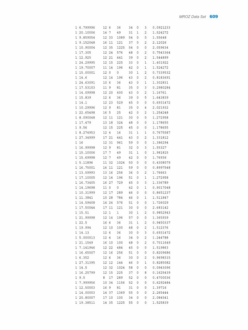
1 6.799996 12 6 36 34 0 3 0.0921233 1 20.10006 14 7 49 31 1 2 1.524272 1 9.859054 12 33 1089 54 0 0 1.55648 1 9.152048 16 11 121 37 0 2 2.12026 1 10.90004 12 35 1225 54 0 0 2.059634 1 17.305 12 24 576 48 0 2 0.7543364 1 12.925 12 21 441 39 0 2 1.544899 1 24.29995 12 15 225 33 0 1 1.401922 1 19.70007 11 14 196 42 0 1 1.524272 1 15.00001 12 0 0 30 1 2 0.7339532 1 14.6 12 14 196 43 0 2 0.8183691 1 24.63091 10 6 36 43 0 1 1.302831 1 17.53103 11 9 81 35 0 3 0.2980284 1 14.09998 12 20 400 43 0 2 1.16761 1 15.839 12 6 36 39 0 5 1.643839 1 14.1 12 23 529 45 0 0 0.6931472 1 10.29996 12 9 81 35 0 4 2.021932 1 22.65498 16 5 25 42 0 2 1.254248 1 8.090048 12 11 121 30 0 0 1.272958 1 17.479 13 18 324 48 0 0 1.178655 1 9.56 12 15 225 45 0 0 1.178655 1 8.274953 12 4 16 31 1 1 0.7675587 1 27.34999 17 21 441 43 0 2 1.331812 1 16 12 31 961 59 0 0 1.386294 1 16.99998 12 9 81 32 0 3 1.55327 1 15.10006 17 7 49 31 1 0 1.981815 1 15.69998 12 7 49 42 0 0 1.76936 1 5.11896 11 32 1024 50 0 0 0.4308079 1 16.75001 16 11 121 59 0 0 0.8997548 1 13.59993 13 16 256 36 0 2 1.76663 1 17.10005 12 14 196 51 0 1 1.272958 1 16.73405 16 27 729 45 0 3 1.336789 1 14.19698 11 0 0 42 0 1 0.9017048 1 10.31999 12 17 289 46 0 0 0.8651237 1 11.3841 10 28 784 46 0 1 1.511847 1 14.59408 14 24 576 51 0 0 1.726029 1 17.50044 17 11 121 30 0 0 2.683142 1 15.51 12 1 1 30 1 2 0.9852943 1 21.99998 12 14 196 57 0 0 1.365939 1 22.5 16 6 36 31 1 2 0.9450337 1 19.994 12 10 100 48 0 2 1.512376 1 14.13 12 6 36 30 0 3 0.6931472 1 5.000013 12 4 16 34 0 2 1.244788 1 21.1549 16 10 100 48 0 2 0.7011649 1 7.141946 12 22 484 45 0 0 1.519863 1 16.65007 12 16 256 51 0 0 0.8209686 1 6.352 12 6 36 30 0 2 0.9698315 1 27.31395 12 12 144 46 0 1 0.8285082 1 14.5 12 32 1024 58 0 0 0.0943096 1 16.25799 12 15 225 37 0 8 0.1625439 1 9.5 8 17 289 52 0 0 0.4700036 1 7.999956 10 34 1156 52 0 0 0.6292484 1 12.50003 16 9 81 31 0 0 1.39716 1 14.00003 14 37 1369 55 0 0 2.265444 1 20.80007 17 10 100 34 0 0 2.084541 1 19.38511 14 35 1225 55 0 0 1.525839
MROZ Data Set 609
1 12.38699 12 6 36 39 0 2 0.7621601 1 28.5 14 19 361 40 0 3 1.481605 1 15.04991 12 10 100 43 0 4 1.262826 1 10.49998 8 11 121 48 0 0 0.9996756 1 11.81 12 15 225 47 0 0 1.832582 1 6.950073 12 12 144 41 0 4 2.479308 1 12.41997 8 12 144 36 0 0 1.279015 1 17.4 17 14 196 46 0 2 1.937936 1 15.5 12 11 121 34 0 0 1.070453 1 21.21704 12 9 81 41 0 3 1.123923 1 18 12 24 576 51 0 1 1.321756 1 11.89992 12 12 144 33 0 0 1.745 1 26.75196 12 13 169 52 0 0 1.301744 1 12.14996 9 29 841 58 0 0 1.641866 1 10.19999 10 11 121 34 2 4 2.10702 1 8.120015 12 13 169 31 0 1 1.467068 1 10.65996 12 19 361 48 0 1 1.605811 1 18.10001 12 2 4 32 0 2 -1.029739 1 8.599986 17 24 576 49 0 0 1.087686 1 13.665 15 9 81 32 2 2 0 1 32.34996 12 6 36 58 0 0 0.9382087 1 12.08501 6 22 484 50 0 0 -0.1505904 1 12.15 14 30 900 60 0 0 0 1 17.69502 12 10 100 50 0 1 1.073671 1 24.7 14 6 36 56 0 0 1.265848 1 2.133992 9 29 841 51 0 0 0.486369 1 20.95005 17 29 841 54 0 1 2.12026 1 10.50008 13 36 1296 59 0 0 1.129853 1 10.55 9 19 361 46 0 2 0.9932518 1 45.75 15 8 64 46 0 1 1.658628 1 13.63204 12 13 169 39 1 3 0.3474122 1 18.23894 12 16 256 44 0 2 1.568324 1 17.09 12 11 121 33 2 0 0.5108456 1 30.2349 12 15 225 33 1 2 0.1148454 1 28.7 12 6 36 48 0 2 -0.6931472 1 19.63 12 13 169 31 0 4 -0.3364523 1 12.82494 12 22 484 45 0 1 1.028226 1 23.8 12 24 576 45 0 1 1.580689 1 26.30003 13 2 4 32 0 2 0.5558946 1 20.69991 12 6 36 47 0 0 0.9014207 1 26 13 2 4 34 0 2 0.8843046 1 10.87702 12 2 4 37 0 1 0.4282046 1 25.61206 12 14 196 36 0 1 1.058415 1 20.98899 12 9 81 47 1 2 0.8783396 1 70.74993 16 11 121 48 0 1 1.654908 1 17.05 12 9 81 42 0 2 1.321756 1 21 13 6 36 33 0 3 0.3285121 1 8.12 11 19 361 46 0 0 1.386294 1 20.88599 12 26 676 47 0 3 1.172885 1 17.66892 12 19 361 44 0 1 1.224187 1 25.20003 12 3 9 36 0 4 0.2876571 1 14.24501 17 7 49 31 2 0 2.230262 1 14.3 14 28 784 55 0 0 1.504077 1 23.70001 16 13 169 45 0 1 1.531152 1 46 17 9 81 47 0 0 1.375158 1 42.9999 12 15 225 46 0 3 1.760269
610 Appendix 1 / Input Data Sets for Task Examples
1 14.749 11 20 400 49 0 0 -0.6931472 1 16.15005 12 29 841 49 0 0 1.406489 1 17.774 12 9 81 45 0 2 1.791759 1 91 17 1 1 38 1 3 1.299292 1 22.29993 10 8 64 47 0 0 1.351004 1 34.60001 13 19 361 54 0 3 1.016281 1 9.620002 11 23 529 41 0 0 1.075344 1 10.89995 12 3 9 43 0 2 1.478965 1 14.49994 16 13 169 31 1 1 1.689487 1 22.00002 17 8 64 47 0 0 2.288598 1 17.90008 12 17 289 35 0 2 -1.822631 1 23.67506 16 4 16 45 0 3 -0.9607652 1 11.79996 12 15 225 33 1 0 1.290994 1 16.14195 16 11 121 54 0 1 0.8648711 1 18.39997 8 7 49 35 0 4 1.540452 1 15.49995 12 0 0 31 1 2 0.6162121 1 17.324 12 0 0 55 0 0 1.648659 1 19.205 12 10 100 34 0 2 1.193498 1 21.30006 13 8 64 38 0 1 2.143976 1 23.56 11 2 4 45 0 1 0.7244036 1 20.85 12 4 16 47 0 1 0.9416075 1 26.15 12 6 36 39 0 2 0.7827594 1 17 14 18 324 36 1 0 1.832582 1 20.72 12 3 9 33 1 2 1.203963 1 17.00009 12 22 484 50 0 0 1.491645 1 16 12 33 1089 58 0 0 1.892133 1 19.50005 17 28 784 49 0 0 2.130895 1 12 14 23 529 41 0 2 1.480604 1 13.73191 12 27 729 51 0 1 0.8943313 1 27.19999 9 11 121 53 0 0 0.2025325 1 5.315 12 6 36 36 1 2 0.4855078 1 16 12 11 121 46 0 2 1.098612 1 27.87198 12 14 196 36 0 2 1.55327 1 40.00001 14 17 289 53 0 1 0.121598 1 15.90003 16 17 289 40 0 3 2.001804 1 27.49997 17 14 196 42 0 2 1.495037 1 17.02005 15 11 121 33 1 1 0.9052298 1 22.39494 12 7 49 43 0 3 0.6325476 1 11.1 16 8 64 31 1 0 1.386294 1 32.70001 17 6 36 47 0 0 2.102914 1 27.79996 17 8 64 54 0 0 1.959644 1 2.199994 12 4 16 33 1 3 0.5108456 1 19.72095 16 25 625 43 0 0 1.236924 1 9.999988 13 24 576 46 0 1 1.443313 1 13.19997 12 11 121 35 0 3 1.021659 1 12.70897 11 19 361 37 0 3 0.6361535 1 27.30005 16 9 81 37 0 2 1.616453 1 21.2 14 19 361 34 0 3 0.2231435 1 14.4 16 14 196 43 1 0 1.049807 1 20.57596 12 22 484 46 0 0 1.415052 1 12.49999 9 6 36 35 0 3 0.5753766 1 17.50022 17 23 529 46 0 0 2.606682 1 44.00004 14 15 225 46 0 0 1.517915 1 13.11895 12 6 36 43 0 2 0.7550416 1 14.00006 12 11 121 30 0 0 1.094972 1 9.645086 11 2 4 41 0 2 0.9421144
MROZ Data Set 611

1 17.39705 12 22 484 54 0 1 1.724943 1 7.799889 12 10 100 31 0 1 1.031546 1 13.13398 10 14 196 44 0 0 0.4743691 1 25.6 12 12 144 32 0 1 0.8109302 1 13.90003 5 9 81 47 0 0 0.7092666 1 19.29794 17 13 169 46 0 1 1.710549 1 9.200016 11 18 324 37 0 0 0.4602689 1 37.99999 12 8 64 51 0 2 1.331812 1 44 12 11 121 49 0 1 1.098612 1 21.37202 14 9 81 36 0 4 2.157999 1 23.66802 11 9 81 39 0 1 1.437581 1 9 12 14 196 48 0 2 1.544899 1 25.19995 14 9 81 38 0 2 1.410597 1 21.22 12 2 4 40 0 2 3.218876 1 33.96991 10 12 144 39 1 5 0.9681619 1 17.07 16 15 225 37 0 0 1.791759 1 6.016024 13 11 121 49 0 1 1.68873 1 17.10001 12 7 49 33 0 3 -0.409172 1 8.237 12 9 81 30 0 0 0.2231435 1 13.30008 12 19 361 54 0 0 0.8221558 1 16.00002 11 11 121 39 0 4 1.241702 1 12.53999 12 8 64 43 0 3 1.427124 1 18.00004 9 13 169 31 0 3 1.497097 1 31.2 13 4 16 33 0 3 0.5596158 1 20.74991 12 7 49 40 0 3 1.300028 1 11.09992 12 19 361 36 0 1 1.88443 1 20.68 12 14 196 51 0 0 0.9555114 1 18.00001 13 14 196 44 0 1 1.582087 1 32.43007 16 3 9 42 0 3 1.755614 1 32.90003 12 9 81 40 0 1 1.513103 1 24.10001 16 7 49 34 1 1 2.251892 1 17.80039 17 7 49 30 0 0 2.364432 1 20.50002 12 14 196 54 0 0 0.1053505 1 10.4999 12 29 841 51 0 0 1.399729 1 10.43703 9 19 361 44 0 2 0.9884625 1 18.19499 12 14 196 43 0 1 1.090647 1 12.84508 12 16 256 34 0 1 1.154614 1 13.8 13 10 100 45 0 0 1.266948 1 22.2 12 12 144 39 0 0 2.885192 1 6.699941 12 24 576 50 0 0 1.22888 1 6.250016 12 6 36 52 0 0 1.203963 1 15.60001 12 9 81 41 0 2 1.35738 1 3.30001 10 14 196 59 0 0 0.8377236 1 3.670978 12 26 676 52 0 0 0.5369611 1 7.789997 16 7 49 46 0 0 0.7487238 1 18.27199 12 4 16 41 1 5 2.295873 1 10.95398 11 15 225 33 0 2 1.107803 1 13.49999 12 23 529 45 0 0 0.6208453 1 11.20001 10 1 1 36 1 2 -2.054164 1 20.99991 12 29 841 48 0 1 1.892012 1 25.7 12 9 81 47 0 1 1.729725 1 8.932994 12 6 36 45 0 0 0.4693784 1 19.15998 12 11 121 37 0 2 0.9808417 1 26.58999 16 17 289 46 0 4 2.069492 1 22.40001 17 6 36 43 0 3 1.675188 1 20.633 12 7 49 42 0 2 1.386294
612 Appendix 1 / Input Data Sets for Task Examples
1 28.20001 17 2 4 34 1 2 1.799215 1 28.8 12 24 576 52 0 0 1.832582 1 8.999997 12 4 16 37 0 3 1.090647 1 11.39994 12 11 121 37 0 1 1.443124 1 10.40001 8 25 625 52 0 0 1.25036 1 19.08006 12 11 121 30 1 0 1.602313 1 9.46604 13 2 4 31 0 1 1.018559 1 6.50006 12 19 361 38 0 1 1.297053 1 29.11701 12 7 49 43 0 3 1.685194 1 19.10302 8 2 4 49 0 1 -0.4209849 1 16.34997 12 20 400 55 0 0 1.562095 1 32.02502 17 10 100 38 0 2 2.146528 1 16.70006 17 19 361 52 0 0 2.347463 1 4.811038 12 17 289 48 0 0 0.9698315 1 24.62601 13 12 144 32 0 2 1.924146 1 17.40001 12 11 121 32 0 1 1.626728 1 13.02504 12 6 36 38 0 2 -0.0392607 1 19.00698 12 10 100 46 0 3 1.460149 1 14.03 12 4 16 40 0 3 1.955394 1 14.89991 9 2 4 31 0 4 0.9263599 1 25.00006 10 13 169 43 0 1 2.066192 1 10.70007 12 21 441 51 0 0 1.422843 1 24.25 16 9 81 30 1 0 2.101032 1 39.13997 13 4 16 52 0 0 2.261461 1 7.199973 8 2 4 30 1 5 0.7013138 1 31.811 16 19 361 51 0 0 2.031013 1 10.00005 13 4 16 31 0 2 1.162369 1 20.66 12 9 81 34 0 4 0.4700036 1 13.49998 11 14 196 49 0 0 1.410597 1 25.38 13 6 36 35 1 3 0.3930551 1 18.27498 12 24 576 53 1 0 1.290994 1 39.213 12 1 1 32 0 3 0 1 10.49994 10 13 169 38 0 3 0.9571255 1 34.857 12 3 9 54 0 0 0.5596158 1 28.502 17 10 100 47 0 1 1.568616 1 12.99996 15 16 256 45 0 1 1.710188 1 41.39991 16 9 81 47 0 1 1.410597 1 14.78 10 19 361 59 0 0 0.2231435 1 15.05 11 4 16 32 0 1 0.5108456 1 29.69998 12 10 100 45 0 1 1.332392 1 16.16502 12 5 25 40 0 4 0.8601859 1 25.20516 14 7 49 47 0 2 2.32278 1 14.2 16 3 9 36 1 2 1.919595 1 18.15897 14 38 1444 56 0 0 1.976107 1 28.98106 8 16 256 41 0 1 0.8954347 1 13.392 7 13 169 48 0 3 0.1812376 1 9.17502 12 1 1 36 1 2 0.4953058 1 27.03985 12 7 49 41 0 0 0.5777924 1 13.14995 14 15 225 41 0 0 1.078818 1 16.40007 12 10 100 36 0 3 1.603199 1 21.29999 12 2 4 37 0 3 0.6208453 1 17.20102 12 19 361 38 0 0 2.083894 1 8.560026 14 25 625 43 0 2 1.379169 1 6.49084 16 25 625 54 0 0 1.112384 1 12.49997 12 7 49 38 0 1 1.067122 1 27.00002 12 15 225 30 1 0 1.118807
MROZ Data Set 613
1 53.50005 12 11 121 49 0 0 1.588541 1 52.49995 13 25 625 45 0 1 1.390311 1 38.39998 13 19 361 51 0 0 1.714806 1 13.89194 10 4 16 34 0 0 0.2010615 1 3.899993 12 14 196 34 0 2 0.987271 1 34.2 12 19 361 41 0 1 0.9835007 1 19.70008 12 18 324 49 0 1 2.233171 1 18.49995 12 14 196 32 0 0 1.143618 1 10.99998 14 11 121 32 0 0 -0.6113829 1 43.30001 17 4 16 32 0 2 2.153052 1 18.76001 10 29 841 47 0 0 1.299837 1 4.800096 9 21 441 39 0 1 0.8409204 1 21.5 12 24 576 49 0 0 1.058484 1 28.03994 12 19 361 37 0 3 1.152658 1 26 16 31 961 59 0 0 1.293576 1 27 12 28 784 50 0 0 1.832582 1 17.79969 17 15 225 32 0 1 2.32718 1 17.40195 12 27 729 46 0 0 1.166146 1 19.30999 17 13 169 43 0 2 2.034993 1 9.99998 11 4 16 37 0 3 0.6792511 1 11.17998 16 10 100 32 0 2 1.547137 1 18.85696 11 8 64 39 0 1 0.7530186 1 12.30002 13 4 16 34 0 2 0.8472836 1 13.67712 11 18 324 39 0 1 0.871126 1 9.559997 8 3 9 45 0 3 0.2282505 1 24.49998 11 11 121 50 0 0 0.0896578 1 23.15 12 8 64 40 0 1 1.321756 1 15.59088 10 10 100 30 0 1 1.196102 1 14.42092 17 33 1089 57 0 0 1.636119 1 17.45491 12 19 361 39 0 1 1.892012 1 9.800019 12 35 1225 53 0 0 1.518309 1 17.57446 17 21 441 48 0 1 2.472159 1 16.555 14 7 49 46 0 1 1.321756 1 13.29497 12 18 324 47 0 0 1.473641 1 11.844 12 4 16 43 0 1 1.369479 1 46.64506 12 12 144 47 0 0 1.203963 1 14.69999 12 16 256 47 0 1 1.198729 1 26.09008 12 14 196 47 0 0 1.27021 1 9.9 12 3 9 46 0 0 0.4700036 1 9.048026 9 1 1 34 0 4 0.7999817 1 30.75006 10 27 729 48 0 0 1.565946 1 8.49994 12 12 144 30 0 1 1.758978 1 22.24999 12 6 36 51 0 1 0.8580258 1 42.91 12 9 81 52 0 5 0.6931472 1 33.3 12 2 4 37 0 2 0.6418539 1 13.8199 12 6 36 32 0 2 1.63374 1 23.60001 17 9 81 36 0 2 1.703748 1 13.00007 12 16 256 35 0 2 1.844004 1 20.74994 17 22 484 45 0 0 1.966119 1 6.3 12 26 676 56 0 0 0.8649974 1 7.788925 10 11 121 40 0 2 0.9333052 1 10.47004 12 11 121 45 1 2 0.7792332 1 12 12 15 225 32 0 2 0.9555114 1 16.97992 12 13 169 45 0 0 1.316247 1 17.9 12 6 36 40 0 2 1.475906 1 15.53994 12 20 400 38 0 1 1.491397
614 Appendix 1 / Input Data Sets for Task Examples
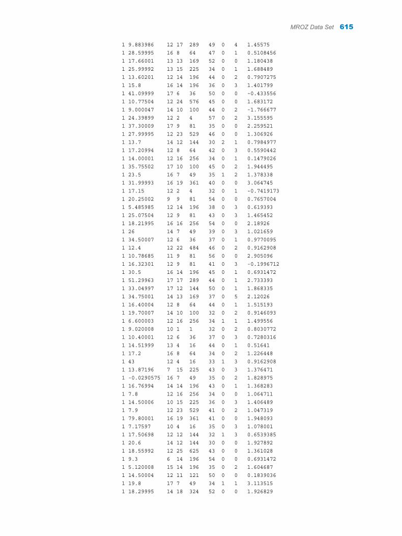
1 9.883986 12 17 289 49 0 4 1.45575 1 28.59995 16 8 64 47 0 1 0.5108456 1 17.66001 13 13 169 52 0 0 1.180438 1 25.99992 13 15 225 34 0 1 1.688489 1 13.60201 12 14 196 44 0 2 0.7907275 1 15.8 16 14 196 36 0 3 1.401799 1 41.09999 17 6 36 50 0 0 -0.433556 1 10.77504 12 24 576 45 0 0 1.683172 1 9.000047 14 10 100 44 0 2 -1.766677 1 24.39899 12 2 4 57 0 2 3.155595 1 37.30009 17 9 81 35 0 0 2.259521 1 27.99995 12 23 529 46 0 0 1.306926 1 13.7 14 12 144 30 2 1 0.7984977 1 17.20994 12 8 64 42 0 3 0.5590442 1 14.00001 12 16 256 34 0 1 0.1479026 1 35.75502 17 10 100 45 0 2 1.944495 1 23.5 16 7 49 35 1 2 1.378338 1 31.99993 16 19 361 40 0 0 3.064745 1 17.15 12 2 4 32 0 1 -0.7419173 1 20.25002 9 9 81 54 0 0 0.7657004 1 5.485985 12 14 196 38 0 3 0.619393 1 25.07504 12 9 81 43 0 3 1.465452 1 18.21995 16 16 256 54 0 0 2.18926 1 26 14 7 49 39 0 3 1.021659 1 34.50007 12 6 36 37 0 1 0.9770095 1 12.4 12 22 484 46 0 2 0.9162908 1 10.78685 11 9 81 56 0 0 2.905096 1 16.32301 12 9 81 41 0 3 -0.1996712 1 30.5 16 14 196 45 0 1 0.6931472 1 51.29963 17 17 289 44 0 1 2.733393 1 33.04997 17 12 144 50 0 1 1.868335 1 34.75001 14 13 169 37 0 5 2.12026 1 16.40004 12 8 64 44 0 1 1.515193 1 19.70007 14 10 100 32 0 2 0.9146093 1 6.600003 12 16 256 34 1 1 1.499556 1 9.020008 10 1 1 32 0 2 0.8030772 1 10.40001 12 6 36 37 0 3 0.7280316 1 14.51999 13 4 16 44 0 1 0.51641 1 17.2 16 8 64 34 0 2 1.226448 1 43 12 4 16 33 1 3 0.9162908 1 13.87196 7 15 225 43 0 3 1.376471 1 -0.0290575 16 7 49 35 0 2 1.828975 1 16.76994 14 14 196 43 0 1 1.368283 1 7.8 12 16 256 34 0 0 1.064711 1 14.50006 10 15 225 36 0 3 1.406489 1 7.9 12 23 529 41 0 2 1.047319 1 79.80001 16 19 361 41 0 0 1.948093 1 7.17597 10 4 16 35 0 3 1.078001 1 17.50698 12 12 144 32 1 3 0.6539385 1 20.6 14 12 144 30 0 0 1.927892 1 18.55992 12 25 625 43 0 0 1.361028 1 9.3 6 14 196 54 0 0 0.6931472 1 5.120008 15 14 196 35 0 2 1.604687 1 14.50004 12 11 121 50 0 0 0.1839036 1 19.8 17 7 49 34 1 1 3.113515 1 18.29995 14 18 324 52 0 0 1.926829
MROZ Data Set 615
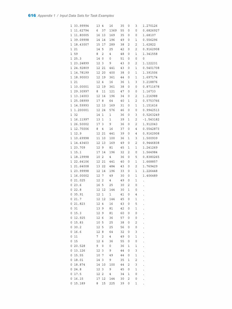
1 33.99994 13 4 16 35 0 3 1.270126 1 11.62794 6 37 1369 55 0 0 0.6826927 1 11.80005 16 13 169 35 0 0 1.68107 1 39.09998 14 14 196 49 0 1 0.556296 1 18.43007 15 17 289 38 2 2 1.62822 1 21 14 5 25 42 0 2 0.9162908 1 59 8 2 4 48 0 1 1.341558 1 25.3 14 0 0 51 0 0 0 1 23.24899 12 3 9 43 0 2 1.122231 1 24.92809 12 21 441 43 0 1 0.5401708 1 14.78199 12 20 400 38 0 1 1.391506 1 18.90003 12 19 361 44 0 1 1.697174 1 21 12 4 16 36 1 3 3.218876 1 10.00001 12 19 361 38 0 0 0.8711678 1 29.30997 8 11 121 47 0 0 1.16733 1 13.14003 12 14 196 34 0 2 1.216988 1 25.08999 17 8 64 40 1 2 0.5753766 1 14.59993 12 13 169 31 0 1 1.151616 1 1.200001 12 24 576 46 0 0 0.9942513 1 32 14 1 1 36 0 3 0.5263249 1 16.11997 13 1 1 39 1 2 -1.543182 1 26.50002 17 3 9 36 0 2 1.912043 1 12.75006 8 4 16 37 0 4 0.5542873 1 12.9 12 21 441 39 0 4 0.9162908 1 10.69998 11 10 100 36 1 3 1.500939 1 14.43403 12 13 169 49 0 2 0.9446838 1 23.709 12 9 81 45 1 1 1.241269 1 15.1 17 14 196 32 2 0 1.564984 1 18.19998 10 2 4 36 0 5 0.8380265 1 22.64106 12 21 441 40 0 1 1.668857 1 21.64008 13 22 484 43 0 2 1.769429 1 23.99998 12 14 196 33 0 1 1.226448 1 16.00002 12 7 49 30 0 1 1.406489 0 21.025 12 2 4 49 0 1 . 0 23.6 16 5 25 30 2 0 . 0 22.8 12 12 144 30 1 0 . 0 35.91 12 1 1 41 0 4 . 0 21.7 12 12 144 45 0 1 . 0 21.823 12 4 16 43 0 5 . 0 31 13 9 81 42 0 1 . 0 15.3 12 9 81 60 0 0 . 0 12.925 12 6 36 57 0 0 . 0 15.83 10 5 25 38 0 2 . 0 30.2 12 5 25 56 0 0 . 0 16.6 12 8 64 32 0 3 . 0 11 7 2 4 49 0 1 . 0 15 12 6 36 55 0 0 . 0 20.528 9 0 0 36 1 1 . 0 13.126 12 3 9 44 0 3 . 0 15.55 10 7 49 44 0 1 . 0 18.01 14 3 9 35 1 2 . 0 18.874 14 10 100 44 2 3 . 0 24.8 12 3 9 45 0 1 . 0 17.5 12 2 4 34 1 0 . 0 16.15 17 12 144 30 2 0 . 0 15.189 8 15 225 39 0 1 .
616 Appendix 1 / Input Data Sets for Task Examples
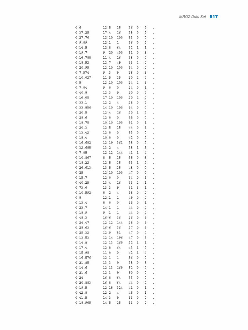
0 6 12 5 25 36 0 2 . 0 37.25 17 4 16 38 0 2 . 0 27.76 12 10 100 53 0 0 . 0 9.09 12 1 1 36 0 2 . 0 14.5 12 8 64 32 1 1 . 0 19.7 9 20 400 51 0 3 . 0 16.788 11 4 16 38 0 0 . 0 18.52 12 7 49 33 2 0 . 0 20.95 12 10 100 54 0 0 . 0 7.574 9 3 9 38 0 3 . 0 10.027 11 5 25 30 2 2 . 0 5 12 10 100 34 2 3 . 0 7.04 9 0 0 34 0 1 . 0 40.8 12 3 9 50 0 2 . 0 16.05 17 10 100 30 2 0 . 0 33.1 12 2 4 38 0 2 . 0 33.856 14 10 100 54 0 0 . 0 20.5 12 4 16 30 1 2 . 0 28.6 12 0 0 55 0 0 . 0 18.75 10 10 100 51 0 1 . 0 20.3 12 5 25 44 0 1 . 0 13.42 12 0 0 53 0 0 . 0 18.4 10 0 0 42 0 2 . 0 16.682 12 19 361 38 0 2 . 0 32.685 13 2 4 38 1 3 . 0 7.05 12 12 144 41 1 4 . 0 10.867 8 5 25 35 0 3 . 0 18.22 12 5 25 33 1 2 . 0 26.613 13 5 25 48 0 0 . 0 25 12 10 100 47 0 0 . 0 15.7 12 0 0 34 0 5 . 0 40.25 13 4 16 33 2 1 . 0 73.6 13 3 9 31 3 1 . 0 10.592 8 2 4 58 0 0 . 0 8 12 1 1 49 0 0 . 0 13.4 8 0 0 55 0 1 . 0 23.7 14 1 1 44 0 0 . 0 18.9 9 1 1 44 0 0 . 0 48.3 16 6 36 36 0 3 . 0 24.47 12 12 144 38 0 3 . 0 28.63 16 6 36 37 0 3 . 0 25.32 12 9 81 47 0 0 . 0 13.53 12 14 196 47 0 3 . 0 14.8 12 13 169 32 1 1 . 0 17.4 12 8 64 43 1 2 . 0 15.98 11 0 0 42 1 4 . 0 16.576 12 1 1 56 0 0 . 0 21.85 13 3 9 38 0 5 . 0 14.6 12 13 169 52 0 2 . 0 21.6 12 3 9 50 0 0 . 0 24 16 8 64 33 0 0 . 0 20.883 16 8 64 44 0 2 . 0 19.5 12 18 324 41 0 1 . 0 42.8 12 2 4 45 0 1 . 0 41.5 14 3 9 53 0 0 . 0 18.965 14 5 25 53 0 0 .
MROZ Data Set 617

0 16.1 12 2 4 42 0 1 . 0 14.7 13 10 100 32 2 0 . 0 18.8 12 30 900 56 0 0 . 0 14.75 11 1 1 37 1 3 . 0 21 12 5 25 40 1 2 . 0 35.4 15 8 64 54 0 3 . 0 10.7 7 0 0 53 0 0 . 0 24.5 12 4 16 48 0 1 . 0 17.045 12 2 4 36 1 2 . 0 18.8 12 30 900 57 0 0 . 0 14 12 25 625 51 0 0 . 0 18.214 13 3 9 33 0 4 . 0 20.177 12 20 400 52 0 0 . 0 8.3 10 20 400 56 0 0 . 0 14.2 12 0 0 36 1 2 . 0 21.768 14 15 225 36 1 0 . 0 29.553 12 10 100 46 0 1 . 0 4.35 10 4 16 31 0 3 . 0 24 11 3 9 52 0 0 . 0 18.3 12 10 100 46 0 2 . 0 17.2 12 9 81 35 2 0 . 0 16.476 12 7 49 59 0 0 . 0 13.4 8 12 144 36 0 1 . 0 44.988 7 0 0 51 1 3 . 0 18.2 16 16 256 31 1 0 . 0 28 14 4 16 31 0 2 . 0 11.55 12 7 49 32 1 1 . 0 28.45 16 7 49 35 1 2 . 0 15.096 12 14 196 40 0 3 . 0 8.009 10 2 4 33 1 2 . 0 10.04 7 20 400 54 0 0 . 0 16.7 12 5 25 36 1 1 . 0 8.4 10 10 100 50 0 1 . 0 13 8 20 400 54 0 0 . 0 17.97 11 10 100 48 0 1 . 0 18.45 15 8 64 41 0 4 . 0 31 12 11 121 50 0 4 . 0 24.135 12 3 9 46 0 2 . 0 31.7 13 6 36 42 0 1 . 0 10.19 9 4 16 31 1 2 . 0 21.574 12 4 16 53 0 0 . 0 26.68 12 9 81 51 0 1 . 0 17.7 12 10 100 47 0 1 . 0 29.4 12 3 9 50 0 1 . 0 22.159 6 2 4 37 0 1 . 0 35 12 2 4 30 2 2 . 0 8.63 12 0 0 49 0 0 . 0 17.08 12 8 64 52 0 2 . 0 32.5 12 6 36 47 0 2 . 0 16 12 15 225 49 0 0 . 0 18.85 12 15 225 44 0 4 . 0 17.5 8 9 81 53 0 0 . 0 19.392 12 8 64 30 1 0 . 0 14.45 12 18 324 54 0 2 . 0 21.8 7 3 9 47 1 1 . 0 7.7 15 10 100 56 0 0 .
618 Appendix 1 / Input Data Sets for Task Examples
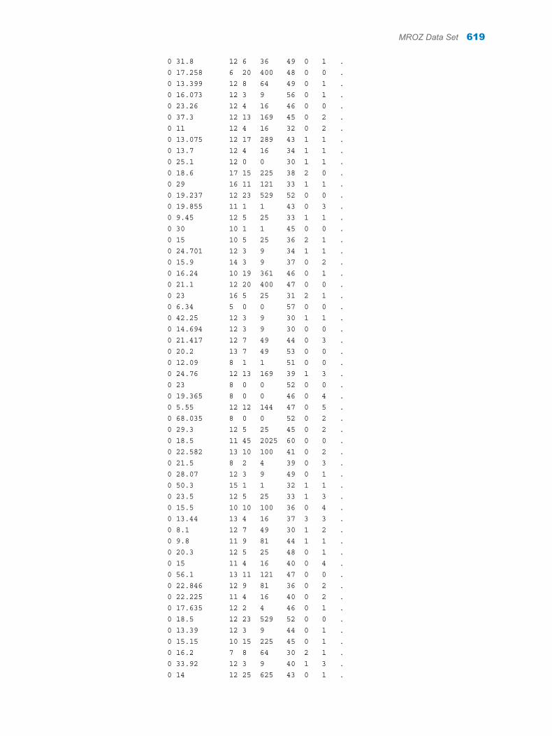
0 31.8 12 6 36 49 0 1 . 0 17.258 6 20 400 48 0 0 . 0 13.399 12 8 64 49 0 1 . 0 16.073 12 3 9 56 0 1 . 0 23.26 12 4 16 46 0 0 . 0 37.3 12 13 169 45 0 2 . 0 11 12 4 16 32 0 2 . 0 13.075 12 17 289 43 1 1 . 0 13.7 12 4 16 34 1 1 . 0 25.1 12 0 0 30 1 1 . 0 18.6 17 15 225 38 2 0 . 0 29 16 11 121 33 1 1 . 0 19.237 12 23 529 52 0 0 . 0 19.855 11 1 1 43 0 3 . 0 9.45 12 5 25 33 1 1 . 0 30 10 1 1 45 0 0 . 0 15 10 5 25 36 2 1 . 0 24.701 12 3 9 34 1 1 . 0 15.9 14 3 9 37 0 2 . 0 16.24 10 19 361 46 0 1 . 0 21.1 12 20 400 47 0 0 . 0 23 16 5 25 31 2 1 . 0 6.34 5 0 0 57 0 0 . 0 42.25 12 3 9 30 1 1 . 0 14.694 12 3 9 30 0 0 . 0 21.417 12 7 49 44 0 3 . 0 20.2 13 7 49 53 0 0 . 0 12.09 8 1 1 51 0 0 . 0 24.76 12 13 169 39 1 3 . 0 23 8 0 0 52 0 0 . 0 19.365 8 0 0 46 0 4 . 0 5.55 12 12 144 47 0 5 . 0 68.035 8 0 0 52 0 2 . 0 29.3 12 5 25 45 0 2 . 0 18.5 11 45 2025 60 0 0 . 0 22.582 13 10 100 41 0 2 . 0 21.5 8 2 4 39 0 3 . 0 28.07 12 3 9 49 0 1 . 0 50.3 15 1 1 32 1 1 . 0 23.5 12 5 25 33 1 3 . 0 15.5 10 10 100 36 0 4 . 0 13.44 13 4 16 37 3 3 . 0 8.1 12 7 49 30 1 2 . 0 9.8 11 9 81 44 1 1 . 0 20.3 12 5 25 48 0 1 . 0 15 11 4 16 40 0 4 . 0 56.1 13 11 121 47 0 0 . 0 22.846 12 9 81 36 0 2 . 0 22.225 11 4 16 40 0 2 . 0 17.635 12 2 4 46 0 1 . 0 18.5 12 23 529 52 0 0 . 0 13.39 12 3 9 44 0 1 . 0 15.15 10 15 225 45 0 1 . 0 16.2 7 8 64 30 2 1 . 0 33.92 12 3 9 40 1 3 . 0 14 12 25 625 43 0 1 .
MROZ Data Set 619
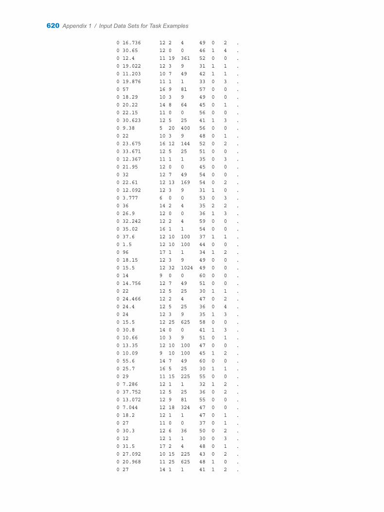
0 16.736 12 2 4 49 0 2 . 0 30.65 12 0 0 46 1 4 . 0 12.4 11 19 361 52 0 0 . 0 19.022 12 3 9 31 1 1 . 0 11.203 10 7 49 42 1 1 . 0 19.876 11 1 1 33 0 3 . 0 57 16 9 81 57 0 0 . 0 18.29 10 3 9 49 0 0 . 0 20.22 14 8 64 45 0 1 . 0 22.15 11 0 0 56 0 0 . 0 30.623 12 5 25 41 1 3 . 0 9.38 5 20 400 56 0 0 . 0 22 10 3 9 48 0 1 . 0 23.675 16 12 144 52 0 2 . 0 33.671 12 5 25 51 0 0 . 0 12.367 11 1 1 35 0 3 . 0 21.95 12 0 0 45 0 0 . 0 32 12 7 49 54 0 0 . 0 22.61 12 13 169 54 0 2 . 0 12.092 12 3 9 31 1 0 . 0 3.777 6 0 0 53 0 3 . 0 36 14 2 4 35 2 2 . 0 26.9 12 0 0 36 1 3 . 0 32.242 12 2 4 59 0 0 . 0 35.02 16 1 1 54 0 0 . 0 37.6 12 10 100 37 1 1 . 0 1.5 12 10 100 44 0 0 . 0 96 17 1 1 34 1 2 . 0 18.15 12 3 9 49 0 0 . 0 15.5 12 32 1024 49 0 0 . 0 14 9 0 0 60 0 0 . 0 14.756 12 7 49 51 0 0 . 0 22 12 5 25 30 1 1 . 0 24.466 12 2 4 47 0 2 . 0 24.4 12 5 25 36 0 4 . 0 24 12 3 9 35 1 3 . 0 15.5 12 25 625 58 0 0 . 0 30.8 14 0 0 41 1 3 . 0 10.66 10 3 9 51 0 1 . 0 13.35 12 10 100 47 0 0 . 0 10.09 9 10 100 45 1 2 . 0 55.6 14 7 49 60 0 0 . 0 25.7 16 5 25 30 1 1 . 0 29 11 15 225 55 0 0 . 0 7.286 12 1 1 32 1 2 . 0 37.752 12 5 25 36 0 2 . 0 13.072 12 9 81 55 0 0 . 0 7.044 12 18 324 47 0 0 . 0 18.2 12 1 1 47 0 1 . 0 27 11 0 0 37 0 1 . 0 30.3 12 6 36 50 0 2 . 0 12 12 1 1 30 0 3 . 0 31.5 17 2 4 48 0 1 . 0 27.092 10 15 225 43 0 2 . 0 20.968 11 25 625 48 1 0 . 0 27 14 1 1 41 1 2 .
620 Appendix 1 / Input Data Sets for Task Examples
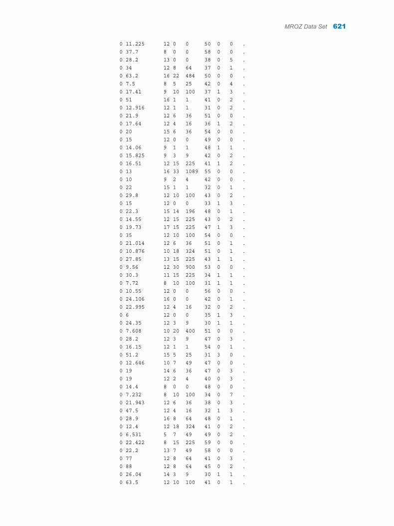
0 11.225 12 0 0 50 0 0 . 0 37.7 8 0 0 58 0 0 . 0 28.2 13 0 0 38 0 5 . 0 34 12 8 64 37 0 1 . 0 63.2 16 22 484 50 0 0 . 0 7.5 8 5 25 42 0 4 . 0 17.41 9 10 100 37 1 3 . 0 51 16 1 1 41 0 2 . 0 12.916 12 1 1 31 0 2 . 0 21.9 12 6 36 51 0 0 . 0 17.64 12 4 16 36 1 2 . 0 20 15 6 36 54 0 0 . 0 15 12 0 0 49 0 0 . 0 14.06 9 1 1 48 1 1 . 0 15.825 9 3 9 42 0 2 . 0 16.51 12 15 225 41 1 2 . 0 13 16 33 1089 55 0 0 . 0 10 9 2 4 42 0 0 . 0 22 15 1 1 32 0 1 . 0 29.8 12 10 100 43 0 2 . 0 15 12 0 0 33 1 3 . 0 22.3 15 14 196 48 0 1 . 0 14.55 12 15 225 43 0 2 . 0 19.73 17 15 225 47 1 3 . 0 35 12 10 100 54 0 0 . 0 21.014 12 6 36 51 0 1 . 0 10.876 10 18 324 51 0 1 . 0 27.85 13 15 225 43 1 1 . 0 9.56 12 30 900 53 0 0 . 0 30.3 11 15 225 34 1 1 . 0 7.72 8 10 100 31 1 1 . 0 10.55 12 0 0 56 0 0 . 0 24.106 16 0 0 42 0 1 . 0 22.995 12 4 16 32 0 2 . 0 6 12 0 0 35 1 3 . 0 24.35 12 3 9 30 1 1 . 0 7.608 10 20 400 51 0 0 . 0 28.2 12 3 9 47 0 3 . 0 16.15 12 1 1 54 0 1 . 0 51.2 15 5 25 31 3 0 . 0 12.646 10 7 49 47 0 0 . 0 19 14 6 36 47 0 3 . 0 19 12 2 4 40 0 3 . 0 14.4 8 0 0 48 0 0 . 0 7.232 8 10 100 34 0 7 . 0 21.943 12 6 36 38 0 3 . 0 47.5 12 4 16 32 1 3 . 0 28.9 16 8 64 48 0 1 . 0 12.4 12 18 324 41 0 2 . 0 6.531 5 7 49 49 0 2 . 0 22.422 8 15 225 59 0 0 . 0 22.2 13 7 49 58 0 0 . 0 77 12 8 64 41 0 3 . 0 88 12 8 64 45 0 2 . 0 26.04 14 3 9 30 1 1 . 0 63.5 12 10 100 41 0 1 .
MROZ Data Set 621
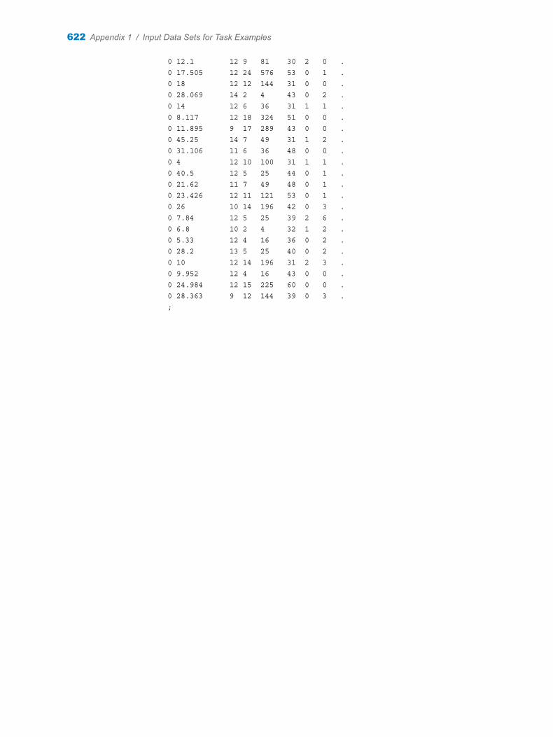
0 12.1 12 9 81 30 2 0 . 0 17.505 12 24 576 53 0 1 . 0 18 12 12 144 31 0 0 . 0 28.069 14 2 4 43 0 2 . 0 14 12 6 36 31 1 1 . 0 8.117 12 18 324 51 0 0 . 0 11.895 9 17 289 43 0 0 . 0 45.25 14 7 49 31 1 2 . 0 31.106 11 6 36 48 0 0 . 0 4 12 10 100 31 1 1 . 0 40.5 12 5 25 44 0 1 . 0 21.62 11 7 49 48 0 1 . 0 23.426 12 11 121 53 0 1 . 0 26 10 14 196 42 0 3 . 0 7.84 12 5 25 39 2 6 . 0 6.8 10 2 4 32 1 2 . 0 5.33 12 4 16 36 0 2 . 0 28.2 13 5 25 40 0 2 . 0 10 12 14 196 31 2 3 . 0 9.952 12 4 16 43 0 0 . 0 24.984 12 15 225 60 0 0 . 0 28.363 9 12 144 39 0 3 . ;
622 Appendix 1 / Input Data Sets for Task Examples
Appendix 2References
Cochran, W. G., and G. M. Cox. 1950. Experimental Designs. New York, NY: Wiley.
De Boor, C. 1978. A Practical Guide to Splines. New York, NY: Springer-Verlag.
Friendly, M. 2000. Visualizing Categorial Data. Cary, NC: SAS Institute Inc.
Goodall, C. 1983. “M-Estimators of Location: An Outline of Theory.” Understanding Robust and Exploratory Data Analysis. Edited by D.C. Hoaglin, M. Mosteller, and J.W. Tukey. New York, NY: John Wiley & Sons.
Hansen, E. 1990. “Making the ‘Complex’ Simple.” Problem-Driven Case Studies in Quality Improvement: Second Annual Symposium, Madison, WI, 7.1.1–7.1.21.
Hilbe, J. M. 2009. Logistic Regression Models. London, England: Chapman & Hall/CRC.
Hosmer, D. W. Jr., and S. Lemeshow. 2000. Applied Logistic Regression. 2 ed. New York, NY: John Wiley & Sons.
Kruskal, J.B. 1964. “Nonmetric Multidimensional Scaling by Optimizing Goodness of Fit to a Nonmetric Hypothesis.” Psychometrika 29: 1–27.
Lawless, J. F., and K. Singhal. 1978. “Efficient Screening of Nonnormal Regression Models.” Biometrics ( 34): 318–327.
Pregibon, D. 1981. “Logistic Regression Diagnostics.” Annals of Statistics ( 9): 705–724.
Rodriguez, R.N. 1996. “Health Care Applications of Statistical Process Control: Examples Using the SAS System.” Proceedings of the Twenty-First Annual SAS Users Group International Conference, Cary, NC, 1381–1396.
Van der Voet, H. 1994. “Comparing the Predictive Accuracy of Models Using a Simple Randomization Test.” Chemometrics and Intelligent Laboratory Systems 25: 313–323.
623

624 Appendix 2 / References

Recommended Readingn SAS Studio: User's Guide
n SAS Studio: Developer's Guide
For a complete list of SAS publications, go to sas.com/store/books. If you have questions about which titles you need, please contact a SAS Representative:
SAS BooksSAS Campus DriveCary, NC 27513-2414Phone: 1-800-727-0025Fax: 1-919-677-4444Email: [email protected] address: sas.com/store/books
625

626 Recommended Reading