sap speaks pddl: exploiting a software-engineering model
TRANSCRIPT

HAL Id: hal-00765034https://hal.inria.fr/hal-00765034
Submitted on 14 Dec 2012
HAL is a multi-disciplinary open accessarchive for the deposit and dissemination of sci-entific research documents, whether they are pub-lished or not. The documents may come fromteaching and research institutions in France orabroad, or from public or private research centers.
L’archive ouverte pluridisciplinaire HAL, estdestinée au dépôt et à la diffusion de documentsscientifiques de niveau recherche, publiés ou non,émanant des établissements d’enseignement et derecherche français ou étrangers, des laboratoirespublics ou privés.
SAP Speaks PDDL: Exploiting a Software-EngineeringModel for Planning in Business Process Management
Joerg Hoffmann, Ingo Weber, Frank Kraft
To cite this version:Joerg Hoffmann, Ingo Weber, Frank Kraft. SAP Speaks PDDL: Exploiting a Software-EngineeringModel for Planning in Business Process Management. Journal of Artificial Intelligence Research,Association for the Advancement of Artificial Intelligence, 2012, 44, pp.587-632. �10.1613/jair.3636�.�hal-00765034�
Journal of Artificial Intelligence Research 44 (2012) 587-632 Submitted 03/12; published 07/12
SAP Speaks PDDL: Exploiting a Software-Engineering
Model for Planning in Business Process Management
Jorg Hoffmann [email protected]
Saarland University, Saarbrucken, Germany
Ingo Weber [email protected]
NICTA, Sydney, Australia
Frank Michael Kraft [email protected]
bpmnforum.net, Germany
Abstract
Planning is concerned with the automated solution of action sequencing problems de-scribed in declarative languages giving the action preconditions and effects. One importantapplication area for such technology is the creation of new processes in Business ProcessManagement (BPM), which is essential in an ever more dynamic business environment. Amajor obstacle for the application of Planning in this area lies in the modeling. Obtain-ing a suitable model to plan with – ideally a description in PDDL, the most commonlyused planning language – is often prohibitively complicated and/or costly. Our core obser-vation in this work is that this problem can be ameliorated by leveraging synergies withmodel-based software development. Our application at SAP, one of the leading vendors ofenterprise software, demonstrates that even one-to-one model re-use is possible.
The model in question is called Status and Action Management (SAM). It describesthe behavior of Business Objects (BO), i.e., large-scale data structures, at a level of ab-straction corresponding to the language of business experts. SAM covers more than 400kinds of BOs, each of which is described in terms of a set of status variables and how theirvalues are required for, and affected by, processing steps (actions) that are atomic from abusiness perspective. SAM was developed by SAP as part of a major model-based softwareengineering effort. We show herein that one can use this same model for planning, thusobtaining a BPM planning application that incurs no modeling overhead at all.
We compile SAM into a variant of PDDL, and adapt an off-the-shelf planner to solvethis kind of problem. Thanks to the resulting technology, business experts may createnew processes simply by specifying the desired behavior in terms of status variable valuechanges: effectively, by describing the process in their own language.
1. Introduction
Business processes are workflows controlling the flow of activities within and between en-terprises (Aalst, 1997). Business process management (BPM) is concerned, amongst otherthings, with the maintenance of these processes. To minimize time-to-market in an evermore dynamic business environment, it is essential to be able to quickly create new pro-cesses. Doing so involves selecting and arranging suitable IT transactions from huge in-
c©2012 AI Access Foundation. All rights reserved.

Hoffmann, Weber & Kraft
frastructures. That is a very difficult and costly task. Our application supports this taskwithin the software framework of SAP1, one of the leading vendors of enterprise software.
A well-known idea in this context, discussed for example by Jonathan, Moore, Stader,Macintosh, and Chung (1999), Biundo, Aylett, Beetz, Borrajo, Cesta, Grant, McCluskey,Milani, and Verfaillie (2003), and Rodriguez-Moreno, Borrajo, Cesta, and Oddi (2007),is to use technology from the field of planning. This is a long-standing sub-area of AI,that allows the user to describe the problem to be solved in a declarative language. Ina nutshell, planning problems come in the form of an initial state, a goal, and a set ofactions, all formulated relative to a set of (typically Boolean or at least finite-domain) statevariables. A solution (or “plan”) is a schedule of actions transforming the initial state intoa state that satisfies the goal. The planning technology solves (in principle) any problemdescribed in that language. By far the most wide-spread planning language is the planningdomain definition language (PDDL) (McDermott, Ghallab, Howe, Knoblock, Ram, Veloso,Weld, & Wilkins, 1998).2
The idea in the BPM context is to annotate each IT transaction with a planning-likedescription formalizing it as an action. This enables planning systems to compose (partsor approximations of) the desired processes fully automatically, i.e., based on minimal userinput specifying from where the process will start (initial state), and what it should achieve(goal). Very closely related ideas have been explored under the name semantic web servicecomposition in the context of the Semantic Web community (e.g., Narayanan & McIlraith,2002; Agarwal, Chafle, Dasgupta, Karnik, Kumar, Mittal, & Srivastava, 2005; Sirin, Parsia,& Hendler, 2006; Meyer & Weske, 2006).
Runtime performance is important in such an application. Typically, the user – a busi-ness expert wishing to create a new process – will be waiting online for the planning outcome.However the most mission-critical question, discussed for example by Kambhampati (2007)and Rodriguez-Moreno et al. (2007), is: How to get the planning model? To be useful, themodel needs to capture the relevant properties of a huge IT infrastructure, at a level ofabstraction that is high-level enough to be usable for business experts, and at the sametime precise enough to be relevant at IT level. Designing such a model is so costly that onewill need good arguments indeed to persuade a manager to embark on that endeavor.
In the present work, we demonstrate that this problem can be ameliorated by leveragingsynergies with model-based software development, thus reducing the additional modelingoverhead caused by planning. In fact, we show that one can – at least in our particularapplication – re-use exactly, one-to-one, models that were built for the purpose of softwareengineering, and thus reduce the modeling overhead to zero.
It has previously been noted, for example by Turner and McCluskey (1994) and Kitchin,McCluskey, and West (2005), that planning languages have commonalities with softwarespecification languages such as B (Schneider, 2001) and OCL (Object Management Group,2006). Now, typically such specification languages are mathematically oriented to describe
1. http://www.sap.com2. There are many variants of planning, and of PDDL. All share concepts similar to the short description we
just stated. However, that description corresponds best to “classical planning”, where (amongst otherthings) there is no uncertainty about the action effects. We will discuss some details in Section 2.1.Throughout the paper, unless we refer to one of the particular planning formalisms defined in here, weuse the term “planning” in a general sense not targeting any particular variant.
588

SAP Speaks PDDL
low-level properties of programs. This stands in contrast with the more abstract modelsneeded to work with business experts. But that is not always so.
As part of a major effort developing a flexible service-oriented (Krafzig, Banke, & Slama,2005; Bell, 2008) IT infrastructure, called SAP Business ByDesign, SAP has developed amodel called Status and Action Management (SAM). SAM describes how “status variables”of Business Objects (BO) change their values when “actions” – IT transactions affectingthe BOs – are executed. BOs in full detail are vastly complex, containing 1000s of datafields and numerous technical-level transactions. SAM captures the more abstract businessperspective, in terms of a smaller number of user-level actions (like “submit” or “reject”),whose behavior is described using preconditions and effects on high-level status properties(like “submitted” or “rejected”). In this way, SAM corresponds to the language of busi-ness users, and is in very close correspondence with common planning languages. SAM isextensive, covering 404 kinds of BOs with 2418 transactions. The model creation in itselfconstitutes a work effort spanning several years, involving, amongst other things, dedicatedmodeling environments and educational training for modelers.
SAM was originally designed for the purpose of model-driven software development,to facilitate the design of the Business ByDesign infrastructure, and changes thereuntoduring its initial development and afterwards. Business ByDesign covers the needs of agreat breadth of different SAP customer businesses, and is flexibly configurable for thesecustomers. That configuration involves, amongst other things, the design of customer-specific processes, appropriately combining the functionalities provided. Describing theproperties of individual processing steps, rather than supplying each BO with a standard life-cycle workflow, SAM is well-suited to support this flexibility. However, the business usersdesigning the processes are typically not familiar with the details of the infrastructure. UsingSAM for planning, we obtain technology that alleviates this problem. As its output, ourtechnology delivers a first version of the desired process, with the relevant IT transactionsand a suitable control-flow. As its input, the technology requires business users only tospecify the desired status changes – in their own language.
The intended meaning of SAM is, to a large extent, the same as in common planningframeworks. There are some subtleties in the treatment of non-deterministic actions. Oneproblem is that many of the non-deterministic actions modeled in SAM have “bad” outcomesthat preclude successful processing of the respective business object (example: “BO datainconsistent”). That problem is aggravated by the fact that, in SAM’s “non-determinism”,repeated executions of the same action are not independent (example: “check BO consis-tency”). We discuss this in detail, and derive a suitable planning formalism. We compileSAM into PDDL, thus creating as a side-effect of our work a new planning benchmark. Ananonymized PDDL version of SAM is publicly available.
On the algorithmic side, we show that minimal changes to an off-the-shelf planner sufficeto obtain good empirical performance. We adapt the well-known deterministic planningsystem FF (Hoffmann & Nebel, 2001) to perform a suitable variant of AO* (Nilsson, 1969,1971). We run its heuristic function on non-deterministic actions simply by acting as ifwe could choose the outcome, i.e., by applying the “all-outcomes determinization” (Yoon,Fern, & Givan, 2007). We run large-scale experiments with this modified FF, on the fullSAM model as used in SAP. We show that runtime performance is satisfactory in the vastmajority of cases; we point out the remaining challenges.
589

Hoffmann, Weber & Kraft
We have also integrated our planning technology into two BPM process modeling en-vironments, making the planning functionality conveniently accessible for non-IT users.Processes (and plans) in these environments are displayed in a human-readable format.Users can specify status variable values, for example the planning goal, in simple intuitivedrop-down menus. One of the environments is integrated as a research extension into thecommercial SAP NetWeaver platform. Having said that, our technology is not yet part ofan actual SAP product; we will discuss this in Section 7.
The treatment of non-deterministic actions, in our formalism and algorithms, is specificto our application context. This notwithstanding, it is plausible that these techniquescould be useful also in other applications dealing with such actions. From a more generalperspective, the contribution of our work is (A) pointing out that it is possible to leveragesoftware-engineering models for planning, and (B) demonstrating that such an applicationcan be realized at one of the major players in the BPM industry, thus providing a large-scale case study. The principle underlying SAM – modeling software artifacts at a level ofabstraction corresponding to business users – is not limited to SAP. Thus our work mayinspire similar approaches in related contexts.
We next give a brief background on planning and BPM. We then discuss the SAM modelin Section 3, explaining its structure, its context at SAP, and the added value of using itfor planning. We design our planning formalization in Section 4, explain our planningalgorithms in Section 5, and evaluate these experimentally in Section 6. Section 7 describesour prototypes at SAP. Section 8 discusses related work, and Section 9 concludes.
2. Background
We introduce the basic concepts relevant to our work. We start with planning, then overviewbusiness process management (BPM) and its connection to planning.
2.1 Planning
There are many variants of planning (for an overview, see Traverso, Ghallab, & Nau, 2005).To handle SAM, we build on a wide-spread classical planning framework, planning withfinite-domain variables (e.g., Backstrom & Nebel, 1995; Helmert, 2006, 2009). We will ex-tend that framework with a particular kind of “non-deterministic” actions, whose semanticsrelates to notions from planning under uncertainty that we outline below.
Definition 1 (Planning Task) A finite-domain planning task is a tuple (X,A, I,G). X
is a set of variables; each x ∈ X is associated with a finite domain dom(x). A is a set ofactions, where each a ∈ A takes the form (prea, eff a) with prea (the precondition) and eff a
(the effect) each being a partial variable assignment. I is a variable assignment representingthe initial state, and G is a partial variable assignment representing the goal.
A fact is a statement x = c where x ∈ X and c ∈ dom(x). We identify partial variableassignments with conjunctions (sets, sometimes) of facts in the obvious way. A state s is acomplete variable assignment. An action a is applicable in s iff s |= prea. If f is a partialvariable assignment, then s ⊕ f is the variable assignment that coincides with f on eachvariable where f is defined, and that coincides with s on the variables where f is undefined.
590
SAP Speaks PDDL
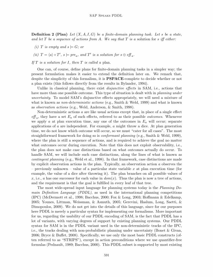
Definition 2 (Plan) Let (X,A, I,G) be a finite-domain planning task. Let s be a state,and let T be a sequence of actions from A. We say that T is a solution for s iff either:
(i) T is empty and s |= G; or
(ii) T = 〈a〉 ◦ T ′, s |= prea, and T ′ is a solution for s⊕ eff a.
If T is a solution for I, then T is called a plan.
One can, of course, define plans for finite-domain planning tasks in a simpler way; thepresent formulation makes it easier to extend the definition later on. We remark that,despite the simplicity of this formalism, it is PSPACE-complete to decide whether or nota plan exists (this follows directly from the results in Bylander, 1994).
Unlike in classical planning, there exist disjunctive effects in SAM, i.e., actions thathave more than one possible outcome. This type of situation is dealt with in planning underuncertainty. To model SAM’s disjunctive effects appropriately, we will need a mixture ofwhat is known as non-deterministic actions (e.g., Smith & Weld, 1999) and what is knownas observation actions (e.g., Weld, Anderson, & Smith, 1998).
Non-deterministic actions a are like usual actions except that, in place of a single effecteff a, they have a set Ea of such effects, referred to as their possible outcomes. Wheneverwe apply a at plan execution time, any one of the outcomes in Ea will occur; separateapplications of a are independent. For example, a might throw a dice. At plan generationtime, we do not know which outcome will occur, so we must “cater for all cases”. The moststraightforward framework for doing so is conformant planning (e.g., Smith & Weld, 1999),where the plan is still a sequence of actions, and is required to achieve the goal no matterwhat outcomes occur during execution. Note that this does not exploit observability, i.e.,the plan does not make case distinctions based on what outcomes actually do occur. Tohandle SAM, we will include such case distinctions, along the lines of what is known ascontingent planning (e.g., Weld et al., 1998). In that framework, case distinctions are madeby explicit observation actions in the plan. Typically, an observation action a observes the– previously unknown – value of a particular state variable x at plan execution time (forexample, the value of a dice after throwing it). The plan branches on all possible values ofx, i.e., a has one successor for each value in dom(x). Thus the plan is now a tree of actions,and the requirement is that the goal is fulfilled in every leaf of that tree.
The most wide-spread input language for planning systems today is the Planning Do-main Definition Language (PDDL), as used in the international planning competitions(IPC) (McDermott et al., 1998; Bacchus, 2000; Fox & Long, 2003; Hoffmann & Edelkamp,2005; Younes, Littman, Weissman, & Asmuth, 2005; Gerevini, Haslum, Long, Saetti, &Dimopoulos, 2009). We do not get into the details of this language, since for our purposeshere PDDL is merely a particular syntax for implementing our formalisms. More importantfor us, regarding the usability of our PDDL encoding of SAM, is the fact that PDDL has alot of variants, with varying degrees of support by existing planning systems. Our PDDLsyntax for SAM is in the PDDL variant used in the non-deterministic tracks of the IPC,i.e., the tracks dealing with non-probabilistic planning under uncertainty (Bonet & Givan,2006; Bryce & Buffet, 2008). Specifically, we use only the most basic PDDL constructs (of-ten referred to as “STRIPS”), except in action preconditions where we use quantifier-freeformulas (Pednault, 1989; Bacchus, 2000). This PDDL subset is supported by most existing
591

Hoffmann, Weber & Kraft
planners, in particular all those based on FF (Hoffmann & Nebel, 2001) or Fast Downward(Helmert, 2006). The limiting factor for planner support are the non-deterministic actions,for which we use the most common syntax, namely the “(oneof eff 1 . . . eff n)” construct fromthe non-deterministic IPC. Non-deterministic actions are supported by only few planners.Further, the semantics we will give to plans using these actions, as fits our application basedon SAM, is non-standard and not supported by existing planners. This notwithstanding,several existing approaches are closely related (cf. Section 8), and, as we show herein, atleast one planner – Contingent-FF (Hoffmann & Brafman, 2005) – can be adapted quiteeasily and successfully to deal with the new semantics.
2.2 Business Process Management
According to the commonly used definition (e.g., Weske, 2007), a business process consistsof a set of activities that are performed in coordination in an organizational and technicalenvironment. These activities jointly realize a business goal. In other words, businessprocesses are how enterprises do business. Business process models serve as an abstractionof the way enterprises do business. For example, a business process model may specifywhich steps are taken, by various entities across an enterprise, to send out a customer quoteanswering a request for quotation. The atomic steps in such a process model may be both,manual steps performed by employees, or automatic steps executed on the IT infrastructure.We will refer to process models simply as “processes”.
An explicit model of processes allows all sorts of support and automation, addressedin the area of business process management (BPM). Herein, we are mostly concerned withprocess creation and adaptation. That is done in BPM modeling environments. Importantly,the users of these environments will typically not be IT experts, but business experts – thepeople familiar with, and taking decisions for, the business. The dominant paradigm forrepresenting business processes are workflows, also called control-flows, often formalizedas Petri nets (e.g., Aalst, 1997). Such a control-flow defines an order of execution forthe process steps, within certain degrees of flexibility implied, for example, by parallelism.For business experts, the control-flow is displayed in a human-readable format, typically aflow diagram. Our application at SAP uses Business Process Modeling Notation (ObjectManagement Group, 2008), short BPMN, which we will illustrate in Section 7.
An alternative paradigm for representing business processes, which relates to the SAMmodel we consider herein, are constraint-based representations (e.g., Wainer & de LimaBezerra, 2003; van der Aalst & Pesic, 2006; Pesic, Schonenberg, Sidorova, & van der Aalst,2007). These model processes implicitly through their desired properties, rather than ex-plicitly through concrete workflows. This kind of representation is more flexible, in that,by modifying the model, we can modify the entire process space. For example, we mightadd a new constraint “archive customer quotes only if all follow-ups have been created”.Such a representation is also more explicit about the reasons for process design, supportinghuman understanding. The downside is that, for actual automated process execution, aconcrete control-flow design is required. One way of viewing our planning technology isthat it provides the service of generating such control-flow designs for SAM.
Processes are executed on IT infrastructures, like the one provided by SAP. Such exe-cution coordinates the individual processing steps, prompting human users as appropriate,and performing all the necessary data updating on IT level. This is realized in dedicated
592

SAP Speaks PDDL
process execution engines (Dumas, ter Hofstede, & van der Aalst, 2005). Clearly, the exe-cution poses high demands on the structure of the workflow. The most basic requirement isthat the atomic process steps correspond to actual steps known to the IT infrastructure.3
The requirements on business processes, such as legal and financial regulations, aresubject to frequent updates. The people responsible for adapting the processes – businessexperts – are not familiar with the IT infrastructure, and may come up with processeswhose “atomic steps” are nowhere near what can be implemented easily, partially overlapwith whole sets of existing functions, and/or require the implementation of new functionsalthough existing functions could have been arranged to do the job. Thus there is a needfor intensive communication between business experts and IT experts, incurring significantcosts for human labor and increased time-to-market.
How can planning come to the rescue? As indicated, the basic (and well-known) ideais to use a planning tool for composing (an approximation of) the process automatically,helping the business expert to come up with a process close to the IT infrastructure. Themain novelty in our work is that we leverage a pre-existing model, SAM, getting us aroundone of the most critical issues in the area: the overhead for creating the planner input.
3. SAM
We explain the structure of the SAM language, and give a running example. We outlinethe background of SAM at SAP, and explain the added value of using SAM for planning.
3.1 SAM Structure and Example
Status and Action Management (SAM) models belong to business objects (BOs). Each BOis associated with a set of finite-domain “status” variables, and with a set of actions. Eachstatus variable highlights one value that the variable will take when a new instance of theBO is created. Each action is described with a textual label (its name), a precondition, andan effect. The precondition and effect are propositional formulas over the variable values.
Definition 3 (SAM BO) A SAM business object o is a triple (X(o), A(o), I(o)). X(o) isa set of status variables; each x ∈ X(o) is associated with a finite domain dom(x). A(o) isa set of actions, where each a(o) ∈ A(o) takes the form (prea(o), eff a(o)); prea(o) (the pre-condition) is a propositional formula over the atoms {x = c | x ∈ X(o), c ∈ dom(x)}; eff a(o)
(the effect) is a negation-free propositional formula over these same atoms, in disjunctivenormal form (DNF). I(o) is a variable assignment representing o’s initial state.
This structure is in obvious correspondence with that of Definition 1. The only differ-ences are that there is no “goal”, and that the preconditions and effects are more complex.In our planning application, the goal is set by the user creating a new process. We discussin Section 4 how to extend Definitions 1 and 2 to handle SAM preconditions and effects.
Note that there are no cross-BO constraints in SAM – each BO o refers only to valuesof its own variables. This is a shortcoming of the current version of SAM: in reality, BOsdo interact. We will get back to this further below.
3. Another important requirement is an appropriate data-flow (van der Aalst, 2003; Dumas et al., 2005),e.g., sending a manager the documents required to decide whether or not to accept a customer quote.Since, in our case, the data is encapsulated into business objects, this is not a major issue for us.
593

Hoffmann, Weber & Kraft
Action name precondition effect
Check CQ Completeness CQ.archiving:notArchived CQ.completeness:complete ORCQ.completeness:notComplete
Check CQ Consistency CQ.archiving:notArchived CQ.consistency:consistent ORCQ.consistency:notConsistent
Check CQ Approval Status CQ.archiving:notArchived AND CQ.approval:necessary ORCQ.approval:notChecked AND CQ.approval:notNecessaryCQ.completeness:complete ANDCQ.consistency:consistent
Decide CQ Approval CQ.archiving:notArchived AND CQ.approval:granted ORCQ.approval:necessary CQ.approval:notGranted
Submit CQ CQ.archiving:notArchived AND CQ.submission:submitted(CQ.approval:notNecessary ORCQ.approval:granted)
Mark CQ as Accepted CQ.archiving:notArchived AND CQ.acceptance:acceptedCQ.submission:submitted
Create Follow-Up for CQ CQ.archiving:notArchived AND CQ.followUp:documentCreatedCQ.acceptance:accepted
Archive CQ CQ.archiving:notArchived CQ.archiving:archived
Figure 1: Our SAM-like running example, modeling the behavior of “customer quotes” CQ.
For illustration, Figure 1 gives a SAM-like model for a BO called “customer quote (CQ)”,that will be our running example. For confidentiality reasons, the shown object and modelare artificial, i.e., they are not contained in SAM as used at SAP. By “CQ.x:c” we denotethe proposition x = c, in the object CQ. The initial state I(CQ) is:
• “CQ.archiving:notArchived”,
• “CQ.completeness:notComplete”,
• “CQ.consistency:notConsistent”,
• “CQ.approval:notChecked”,
• “CQ.submission:notSubmitted”,
• “CQ.acceptance:notAccepted”,
• “CQ.followUp:documentNotCreated”.
When using this example below, where relevant we will assume that the goal entered by theuser is “CQ.followUp:documentCreated AND CQ.archiving:archived”.
The reader should keep in mind that this is merely an illustrative example, which neces-sarily is simple. In particular, the intended life-cycle workflow is rather obvious, given theaction descriptions in Figure 1. This is very much not the case in general. The BusinessObjects modeled in SAM have up to 15 status variables, yielding up to 12 million possiblestates (combinations of variable values) even for a single BO. In other words, SAM is aflexible model – after all, that was its main design purpose – and describes a large num-ber of combination possibilities in a compact way. Furthermore, in two of the applicationscenarios for planning ((A) and (C) in Section 3.3 below), we are actually looking not forentire life-cycles but for process fragments that may begin or end at any BO status values.
594

SAP Speaks PDDL
3.2 SAM@SAP
SAM was created by SAP as part of the development of the IT infrastructure supportingSAP Business ByDesign. That infrastructure constitutes a fully-fledged SAP application.Its key advantage over traditional SAP applications is a higher degree of flexibility, facili-tating the use of SAP software as-a-service. Individual system functions are encapsulatedas software services, using the service-oriented architectures paradigm (Krafzig et al., 2005;Bell, 2008). The software services may be accessed from standard architectures like BPMprocess execution engines, thus enabling their flexible combination with other services. Tofurther support flexibility, the Business ByDesign IT infrastructure is model-driven. IT ar-tifacts at various system levels are described declaratively using SAP-proprietary modelingformats. Business objects are one such IT artifact, and SAM is one such format.
The original purpose of SAM was to facilitate the design, and the management ofchanges, during the development of the Business ByDesign infrastructure (a formidablyhuge enterprise). Of course, SAM also serves the implementation of changes to the infras-tructure later on, should changes be required. New developments are first implemented andtested on the model level. Then parts of the program code are automatically generated fromthe model. Straightforward code skeletons contain the status variables, as well as functionheaders for the available actions (similar to what Eclipse does for Java class definitions). Inaddition, the skeletons are filled with code fragments performing the precondition checksand updates on status variables. Changes pertaining to the status variable level can thusbe implemented in SAM models, and automatically propagated into the code. In this sense,the original semantics of SAM is as follows:
(I) When a BO o is newly created, the values of the status variables are set to I(o).
(II) BO actions a(o) whose precondition prea(o) is not fulfilled are either disallowed, orraise an exception when executed; which one is true depends on the part of thearchitecture attempting to execute the action.
(III) Upon execution of an action a, the status variables change their values as prescribedby one of the disjuncts in the effect DNF eff a(o). The only aspect controlled outsideSAM is which disjunct is chosen: that choice is made based on BO data content notreflected in SAM.
The intention behind SAM is to formulate complex business-level dependencies betweenindividual processing steps, using simple modeling constructs that facilitate easy modifi-cation. The formulation in terms of preconditions and effects relative to high-level statusvariable values was adopted as a natural means to meet these requirements. Of course, thisdesign also took some inspiration from traditional software modeling paradigms (Schneider,2001; Object Management Group, 2006).
Leveraging SAM for planning is a great opportunity because of the effort it takes to buildsuch a model. SAM was developed continuously along with Business ByDesign, across atime span of more than 5 years. Throughout this time, around 200 people were involved (asa part-time occupation) in the development. SAP implemented a dedicated graphical userinterface for this development. There are design patterns for typical cases, there are nam-ing conventions, there is a fully-fledged governance process, and there even is educationaltraining for the developers. A council of senior SAP architects supervises the development.
595
Hoffmann, Weber & Kraft
3.3 Applications of SAM-Based Planning
The Business ByDesign infrastructure is designed to be very general and adaptable, coveringthe needs of a great breadth of different SAP customers’ business domains. To adapt theinfrastructure to their practice, SAP customers may choose to create their own processesas compositions of the functionalities provided (as Web services), in a way tailored to theirneeds. Indeed, a second motivation behind SAM, beside its role for software development,was to facilitate such flexibility, by describing the possible process space in a declarativemanner, rather than imposing standard workflows as is a common methodology in othercontexts such as artefact-centric business process modeling (e.g., Cohn & Hull, 2009). SAMshares this motivation with constraint-based process representation languages. It also sharestheir downside, in that the actual workflows still need to be created. In this context, thereare at least three application scenarios for planning based on SAM:
(A) Development based on SAM. During model-driven development based on SAM,planning enables developers to examine how their changes affect the process space.This greatly facilitates experimentation and testing. For example, planning can beused for debugging, testing whether or not the goal can still be reached, or whetherthe changes opened any unintended possibilities, like, reaching an undesired state ofthe BO (e.g., “CQ.consistency:notConsistent AND CQ.acceptance:accepted”). Morethan such reachability testing (essentially a model checking task), planning serves togenerate entire processes, which as we shall see take the form of BPMN process modelswith parallelism and conditional splits. Developers can examine the space of processesgenerated in this way, determining for different combinations of start/end conditionshow these can be connected. Note that the generality offered by the planning approachis an absolute requirement here – the process generation tool must be at least as generalas SAM, handling propositional formula preconditions and effects.
(B) Designing extended/customized processes. Individual SAP customers have in-dividual requirements on their processes, and thus may use the same BOs in differentways. For example, even if the end state of customer quotes (which in practice aremuch more complex than our illustrative example) always involved being archived,different businesses may differ on the side conditions: one organization only archivesPOs if all follow-ups have been created; another archives only POs that were success-ful; a third organization archives POs immediately and automatically after gettinga response; a fourth only based on an explicit user-request. Part of the motivationbehind SAM is to provide such flexibility. Planning based on SAM can be used toautomatically generate a first version of the desired process.4
(C) Process redesign. Sometimes the best option is to design a new process from scratch.If the business experts doing so are not aware the underlying IT infrastructure, thenthis incurs huge costs at process implementation time. SAM opens the possibilityfor business experts to “explain” the individual steps in the new process in terms ofstatus variable value changes, i.e., in terms of a start/end state corresponding to whatthe business user considers to be an atomic processing step. Planning then showsif and how these status changes can be implemented using existing transactions. In
4. The alternative – equipping each BO with a standard life-cycle or a set thereof – would come at theprize of a flexibility loss for complex BOs, and is not the choice made by SAP.
596

SAP Speaks PDDL
particular, the planner can be called for some business object X (e.g., a sales order)from within a process being created for some other object Y (e.g., a customer quote).Hence, despite the mentioned absence of cross-BO constraints in the current versionof SAM, planning can help to create non-trivial processes spanning several BOs.
All these use cases are supported by our prototype at SAP; we will illustrate its use for (C),in a cross-BO situation as mentioned, in Section 7.3.
An obvious requirement for the planner to be useful is instantaneous response. Typicallya user will be sitting at the computer and waiting for the planner to answer. Further, allfunctionality must be accessible conveniently. In particular, each time a user wants to callthe planner, she needs to provide the planning goal (and possibly the initial state). It isessential that this can be done in a simple and intuitive manner, without in-depth expertisein IT or about the BO the question. Thus we limit ourselves to conjunctive goals in thesense of “I want these status variables to have these values at the end of the process”, likethe goal “CQ.followUp:documentCreated AND CQ.archiving:archived” in our illustrativeexample. In our prototype, such goals are specified using simple drop-down menus.
SAM was not originally intended to do planning, and is of course not perfect for thatpurpose. We will discuss the main limitations in Section 9, but we need to briefly touchon two points here already. The absence of cross-BO constraints in the current versionof SAM has implications for planner setup and performance, and will play a role in ourexperiments.5 Another issue is plan quality. The duration/cost of the actions may differvastly, but SAM does not contain any information about this: it is not relevant to SAM’soriginal purpose, software engineering. We will not address plan quality measures herein.Our planning algorithm of course attempts to find small plans. But it gives no qualityguarantee in that regard, and the practical value of such a guarantee would be doubtful.
4. Planning Formalization
We design the syntax and semantics of a suitable planning formalism capturing SAM, andwe illustrate that formalism using our running example.
4.1 SAM Planning Tasks: Syntax
Given the close correspondence of SAM business objects (Definition 3) with finite-domainplanning tasks (Definition 1), it is straightforward to extend the latter to capture the former.
Definition 4 (SAM Planning Task) A SAM planning task is a tuple (X,A, I,G) whoseelements are the same as in finite-domain planning tasks, except for the action set A. Eacha ∈ A takes the form (prea, Ea) with prea being a propositional formula over the atoms{x = c | x ∈ X, c ∈ dom(x)}, and Ea being a set of partial variable assignments. Themembers eff a ∈ Ea are the outcomes of a.
As discussed above, we keep the goal as simple as possible. For the effects, in place ofthe negation-free propositional DNF formulas of Definition 3, we now have sets Ea of out-comes. The action preconditions are as in Definition 3. This generalizes the partial variable
5. As we shall discuss in Section 9, BO interactions do exist. An according extension of SAM is planned,which could in principle be tackled using the exact same planning technology as presented herein.
597

Hoffmann, Weber & Kraft
assignments from Definition 1 – which are equivalent to negation-free conjunctions over theatoms {x = c | x ∈ X, c ∈ dom(x)} – to arbitrary propositional formulas over these atoms.That generalization poses no issue for defining the plan semantics; at implementation level,most current planning systems compile such preconditions into negation-free conjunctions,using the methods originally proposed by Gazen and Knoblock (1997).
To obtain a SAM planning task (X,A, I,G), when given as input a SAM business objecto = (X(o), A(o), I(o)) along with a goal conjunction G(o), we first set X := X(o), I := I(o),and G := G(o). For each a(o) ∈ A(o) we include one a into A, where prea := prea(o). Asfor eff a(o), we create one partial variable assignment eff a for each disjunct in that DNFformula, and we define the possible outcomes Ea as the set of all these eff a.
By convention, we denote with Ad := {a ∈ A | |Ea| = 1} and And := {a ∈ A | |Ea| > 1}the sets of deterministic and non-deterministic actions of a SAM planning task, respectively.If a ∈ Ad, then by eff a we denote the single outcome of a.
4.2 SAM Planning Tasks: Semantics
SAM action preconditions prea(o) are in direct correspondence with usual planning precon-ditions, cf. point (II) in Section 3.2. By contrast, SAM’s disjunctive effects eff a(o) requireto create a mix of two different kinds of planning actions – non-deterministic actions andobservation actions – from the literature. To understand this, reconsider the role of SAMaction effects eff a(o) in their original environment, i.e., point (III) in Section 3.2. Any oneof the disjuncts will occur, and at plan generation time we do not know which one. At planexecution time, the SAP system executing the action will observe the relevant data content,and will decide which branch to take. In the example from Figure 1, “Check CQ Complete-ness” will answer “CQ.completeness:complete” if the BO data is complete, and will answer“CQ.completeness:notComplete” otherwise. Of course, the SAP system keeps track of whichoutcomes occured. In other words, (a) SAM’s disjunctive effects correspond to observationactions, that (b) internally observe environment data not modeled at the planning level.Due to (a), it makes perfect sense to handle such actions by introducing case distinctionsat plan generation time, one for each outcome. Due to (b), there is no direct link of the“observation” to a reduction of uncertainty at planning level. During execution, the valuesof the “observed variables” are known prior to the “observation” already, and change as aresult of applying that action. For example, “CQ.completeness.notComplete” is consideredto be true prior to the first application of “Check CQ Completeness”, and may be changedto “CQ.completeness.complete” by that action. In that respect, and in that the outcomeset (an arbitrary DNF) is more general than the domain of a particular variable, SAM’sdisjunctive effects are more similar to the common notions of non-deterministic actions.
For simplicity, we will henceforth refer to SAM’s disjunctive-effects actions as non-deterministic actions. Another important point regarding these actions is that data contentis not allowed to change while the process is running; the data is filled in directly upon cre-ation of the BO. Thus the outcome of a non-deterministic action will be the same throughoutthe plan execution, and it makes no sense to execute such an action more than once in aplan. For example, there is no point in repeatedly applying “Check CQ Completeness”.
A final issue is to decide what a “plan” actually is. Cimatti, Pistore, Roveri, and Traverso(2003) describe the three most common concepts, in the presence of non-deterministic ac-
598

SAP Speaks PDDL
tions: strong plans, strong cyclic plans, and weak plans. We will discuss the latter twobelow; the most desirable property is the first one. A strong plan guarantees to reach thegoal no matter which action outcomes occur. We now define this formally, for our setting.
An action tree over A is a tree whose nodes are actions from A, and whose edges arelabeled with partial variable assignments. Each action a in the tree has exactly |Ea| outgoingedges, one for (and labeled with) each eff a ∈ Ea. In the following definitions, And
av refersto the subset of non-deterministic actions that have not yet been used, and are thus stillavailable, at any given state during plan execution. Recall that s⊕eff a, defined in Section 2,over-writes s with those variable values defined in eff a, and leaves s unchanged elsewhere.
Definition 5 (Strong SAM Plan) Let (X,A, I,G) be a SAM planning task with A =Ad ∪ And. Let s be a state, let And
av ⊆ And, and let T be an action tree over A ∪ {STOP}.We say that T is a strong SAM solution for (s,And
av ) iff either:
(i) T consists of the single node STOP, and s |= G; or
(ii) the root of T is a ∈ Ad, s |= prea, and the sub-tree of T rooted at a’s child is a strongSAM solution for (s⊕ eff a, A
ndav ); or
(iii) the root of T is a ∈ Andav , s |= prea, and, for each of a’s children reached via an edge
labeled with eff a ∈ Ea, the sub-tree of T rooted at that child is a strong SAM solutionfor (s⊕ eff a, A
ndav \ {a}).
If T is a strong solution for (I, And), then T is called a strong SAM plan.
Compare this to Definition 2. Item (i) of the present definition is essentially the same,saying that there is nothing to do if the goal is already true. In difference to Definition 2,we then distinguish deterministic actions (ii) and non-deterministic ones (iii). In the formercase, a has a single child and we require the remainder of the tree to solve that child,similarly as in Definition 2. In the latter case, a has several children all of which need to besolved by the respective sub-tree. This corresponds to the desired case distinction observingaction outcomes at plan execution time.
Note that, throughout the plan, there is no uncertainty about the current variable values.Note also that we solve, not a state, but a pair consisting of a state and a subset of non-deterministic actions. This reflects the fact that whether or not an action tree solves a statedepends not only on the state itself, but also on which non-deterministic actions are stillavailable. The maintenance of the set And
av ensures that we allow each non-deterministicaction only once, on each path through T (but the action may occur several times onseparate paths). Thus any one execution of the plan applies the action at most once.
The problem with Definition 5 is that strong plans typically do not exist. To illus-trate this, consider Figure 2, showing a weak SAM plan, a notion we will now formallydefine, for our running example from Figure 1. Recall that the goal is assumed to be“CQ.followUp:documentCreated AND CQ.archiving:archived”. If either of “Check CQCompleteness” or ““Check CQ Consistency”, as shown at the top of Figure 2, result in anegative outcome (“CQ.completeness:notComplete” or “CQ.completeness:notConsistent”),then the goal becomes unreachable. Thus a strong plan does not exist for this SAM plan-ning task. That phenomenon is not limited to this illustrative example. In our experiments,almost 75% of a very large sample of SAM planning tasks did not have a strong plan.
To address this, one can define more complicated goals, or a weaker notion of plans. Forthe former option, one could use goals specifying alternatives, preferences, and/or temporal
599

Hoffmann, Weber & Kraft
Check CQ Completeness
Check CQ Consistency
Check CQ Approval Status
Submit CQ
Y
Y N
N
Mark CQ as Accepted
Archive CQ
notNec Nec
Decide CQ Approval
granted notGranted
Submit CQ
Mark CQ as Accepted
Archive CQ
Create Follow−Up for CQ
Create Follow−Up for CQ
Figure 2: A weak SAM plan for the running example from Figure 1. STOP actions notshown, FAIL actions marked by (red) crosses.
plan properties (e.g., Pistore & Traverso, 2001; Dal Lago, Pistore, & Traverso, 2002; Sha-parau, Pistore, & Traverso, 2006; Gerevini et al., 2009). However, goals will be specifiedonline by business users and it is absolutely essential for this to be as simple as possible.We hence decided to go for the second option.6
The weak plans of Cimatti et al. (2003) are too liberal for our purposes. They guaranteeonly that at least one possible execution of the plan reaches the goal, posing no require-ments on all the other executions. For example, in Figure 2, this would mean to allowthe plan to handle only the left-hand side outcome of “Check CQ Approval Status”, i.e.,“CQ.approval:notNecessary”, and to do nothing at all about (attach the empty tree at) itsother outcome, “CQ.approval:necessary”.
So what about strong cyclic plans? There, the plan may have cycles, provided everyplan state can, in principle, reach the goal. This allows to “wait for a desired outcome”, likea cycle around a dice throw, waiting to obtain a “6”. Alas, repetitions of non-deterministicSAM actions will always produce the same outcome. It is futile to insert a cycle at thetop of Figure 2, waiting for the desired outcome of “Check CQ Completeness”. While it isplausible to prompt a user to edit the BO content and then repeat the check (placeholders forsuch cycles could be inserted as a planning post-process), this is not a suitable exceptionhandling in general. Exception handling depends on the business context, and typicallydepends on the actual customer using the SAP system. This is impossible to reflect in amodel maintained centrally by SAP.
In conclusion, from the perspective of SAM-based planning there is not much one cando other than to highlight the bad outcomes to the user, so that the exception handling can
6. Some works on more complex goals can be employed to define alternative notions of “weak plans” (byusing trivial fall-back goals). We will discuss this in some detail in Section 8.
600

SAP Speaks PDDL
be inserted manually afterwards. Of course, a non-deterministic action should have at leastone successful outcome, or else it would be completely displaced in a process. Further, it isessential to highlight outcomes as “bad” only if they really are “bad”, i.e., to not mark asfailed any outcomes that could actually be solved. Our definition reflects all this:
Definition 6 (Weak SAM Plan) Let (X,A, I,G) be a SAM planning task with A = Ad∪And. Let s be a state, let And
av ⊆ And, and let T be an action tree over A ∪ {STOP ,FAIL}.We say that T is a weak SAM solution for (s,And
av ) iff either:(i) T consists of the single node STOP, and s |= G; or
(ii) the root of T is a ∈ Ad, s |= prea, and the sub-tree of T rooted at a’s child is a weakSAM solution for (s⊕ eff a, A
ndav ); or
(iii) the root of T is a ∈ Andav , s |= prea, and, for each of a’s children reached via an edge
labeled with eff a ∈ Ea, we have that either: (a) the sub-tree of T rooted at that childis a weak SAM solution for (s ⊕ eff a, A
ndav \ {a}); or (b) the sub-tree of T rooted at
that child consists of the single node FAIL, and there exists no action tree T ′ that isa weak SAM solution for (s ⊕ eff a, A
ndav \ {a}); where (a) is the case for at least one
of a’s children.If T is a weak solution for (I, And), then T is called a weak SAM plan.
Compared to Definition 5, the only difference lies in item (iii), which no longer requiresevery child to be solved. Instead, the arrangement of options (a) and (b) means thatfailed nodes – leaves in the tree that stop the plan without success – are tolerated, aslong as at least one child is solved, and every failed node is actually unsolvable. This isin obvious correspondence with our discussion above. In Figure 2, the failed nodes, i.e.,the sub-trees consisting only of the special FAIL action, are crossed out (in red). Notethe difference to Cimatti et al.’s (2003) definition of “weak plans” discussed above: weare not allowed to cross out the right-hand side outcome of “Check CQ Approval Status”,i.e.,“CQ.approval:necessary”, because that outcome is solvable.
We remark that allowing non-deterministic actions only once (or, more generally, havingan upper bound on repetition of non-deterministic actions) is required for Definition 6 tomake sense. In item (iii), the definition recurses on itself when stating that some childrenmay be unsolvable. While such recursion occurs also at other points in Definitions 5 and 6,at those points the action tree T considered is reduced by at least one node. For unsolvablechildren of non-deterministic actions in Definition 6 (iii) (b), such a reduction is not given –the quantification is over any action tree T ′ that may be suitable to solve the child. Whatmakes the recursion sound, instead, is that the set of available non-deterministic actions isdiminished by one. Without this, the notion of “weak SAM plan” would be ill-defined: therecursion step may result in the same planning task over again, allowing the constructionof planning tasks that are considered “solvable” if they are “unsolvable”.7
7. Concretely, say we obtain Definition 6’ from Definition 6 by considering states s only, removing thehandling of And
av . Consider the example with one variable x whose possible values are A and B, withinitial state I : x = A, with goal G : x = B, and with a single action a with two possible outcomes, x = A
or x = B. Say T consists only of a. Then the “bad” outcome of a, i.e., the state x = A, is identical to theoriginal initial state I. If I is “unsolvable” according to Definition 6’, then this outcome of a qualifies forDefinition 6’ (iii) (b), and thus the overall task – the same state I – is considered to be “solvable”. Bycontrast, using Definition 6 as above, the plan must solve the state/available-non-deterministic-actionspair (x = A, {a}), and the bad outcome of a is the different pair (x = A, ∅). That pair is unsolvable, andhence a is a weak plan.
601

Hoffmann, Weber & Kraft
The following observation holds simply because Definition 5 captures a special case ofDefinition 6:
Proposition 1 (Weak SAM Plans Generalize Strong SAM Plans) Let (X,A, I,G)be a SAM planning task with A = Ad ∪ And. Let s be a state, let And
av ⊆ And, and let T bean action tree over A ∪ {STOP}. If T is a strong SAM solution for (s,And
av ), then T is aweak SAM solution for (s,And
av ).
In other words, any strong SAM plan is also a weak SAM plan, and hence in particularany SAM planning task that is solvable under the strong semantics is also solvable underthe weak semantics. The inverse is obviously not true. A counter-example is our runningexample in Figure 2.
We remark that, trivially, deciding whether a plan exists is hard for both, Definition 5and Definition 6. The special case where all actions are deterministic is a generalization ofDefinition 2, where as mentioned that problem is PSPACE-complete.
4.3 SAM Planning Tasks: Running Example
For illustration, we encode our running example, Figure 1, into a SAM planning task(X,A, I,G). We set X := {Arch, Compl , Cons, Appr , Subm, Acc, FoUp}, abbreviat-ing the status variable names mentioned in Figure 1. For example, Arch stands for thevariable “CQ.archiving”. The domain of each of Arch, Compl , Cons, Subm, Acc, and FoUpis {true, false}. This serves to abbreviate the various names used for the respective variablevalues in Figure 1. The domain of Appr is {notChecked ,nec,notNec, granted ,notGranted}.In what follows, for brevity we write facts, i.e., variable/value pairs, involving true/falsevalued variables like literals. For example, we write ¬FoUp instead of (FoUp,no).
The initial state of the SAM BO, and thus the SAM planning task, is:
• I = {¬Arch, ¬Compl , ¬Cons, (Appr ,notChecked), ¬Subm, ¬Acc, ¬FoUp}
The goal is “CQ.followUp:documentCreated AND CQ.archiving:archived”:
• G = {FoUp,Arch}
The deterministic actions Ad are:
• “Mark CQ as Accepted”: (¬Arch ∧ Subm, {Acc})
• “Create Follow-Up for CQ”: (¬Arch ∧Acc, {FoUp})
• “Archive CQ”: (¬Arch, {Arch})
• “Submit CQ”: (¬Arch ∧ ((Appr ,notNec) ∨ (Appr , granted)), {Subm})
Note here that action effects are sets of partial variable assignments, i.e., sets of sets of facts.For the deterministic actions, there is just one partial variable assignment so we omit thesecond pair of set parentheses to avoid notational clutter. Note also that we do not have“delete effects”. The effects assign new values to the affected variables, implicitly removingtheir old values, cf. the meaning of s⊕ eff a as defined in Section 2.
The non-deterministic actions And are:
• Check CQ Completeness: (¬Arch, {{Compl}, {¬Compl}})
• Check CQ Consistency: (¬Arch, {{Cons}, {¬Cons}})
602

SAP Speaks PDDL
• Check CQ Approval Status:
(¬Arch ∧ (Appr ,notChecked) ∧ Compl ∧ Cons, {{(Appr ,nec)}, {(Appr ,notNec)}})
• Decide CQ Approval:
(¬Arch ∧ (Appr ,nec), {{(Appr , granted)}, {(Appr ,notGranted)}})
Figure 2 shows a weak SAM plan for this example. For presentation to the user, a simplepost-process (outlined in Section 7.1) transforms such plans into BPMN workflows.
5. Planning Algorithms
We design an adaptation of FF (Hoffmann & Nebel, 2001), using a variant of the AO* for-ward search from Contingent-FF (Hoffmann & Brafman, 2005), as well as a naıve extensionof FF’s heuristic function. We assume that the reader is familiar with heuristic search ingeneral, and we refer to the literature (e.g., Pearl, 1984) for that background.
5.1 Search
For strong SAM planning – Definition 5 – we use AO* tree search (Nilsson, 1969, 1971).For weak SAM planning – Definition 6 – we use a variant of that search that we refer to asSAM-AO*. We focus in what follows mainly on SAM-AO*, since AO* is well-known andwill become clear as a side effect of the discussion.
Search is forward in an AND-OR tree whose nodes are states (OR nodes) and actions(AND nodes). The OR’ed children of states are the applicable actions, the AND’ed childrenof actions are the alternative outcomes (for deterministic actions, there is a single child sothe AND node trivializes). Like in AO*, we propagate “node solved” and “node failed”markers. The mechanics for this are the usual ones in the case of OR nodes, i.e., the markerof the node is the disjunction of its childrens’ markers. For AND nodes, SAM-AO* differsfrom the usual conjunctive interpretation, implementing the weak SAM planning semanticsof Definition 6: amongst other things, an AND node is failed only if all its children arefailed. Figure 3 provides an overview of SAM-AO*, highlighting the differences to AO*.Figure 4 illustrates the algorithm on a simplification of our running example.
One feature of the algorithm that is immediately apparent is the book-keeping whichnon-deterministic actions are still available. Recall here that, in line with Definitions 5and 6, we allow each non-deterministic action at most once in any execution of a plan. Forthe search algorithm – both in strong planning (AO*) and in weak planning (SAM-AO*) –this means that OR nodes contain not only a state s, but a pair (s,And
av ) giving the state aswell as the subset of And that has not been used up to this node. We will refer to such pairsas search states from now on. The book-keeping of the sets And
av is straightforward. For theinitial state, all non-deterministic actions are still available. Whenever a non-deterministicaction a is applied, for its outcome states, a is no longer available. For illustration, considerhow the action sets are reduced in Figure 4 (B–D).
The heuristic function h, that we assume as a given here, takes as arguments the searchstate, i.e., both the state and the available non-deterministic actions. This is because actionavailability affects goal distance and hence the heuristic estimates. By h(s) = 0 the heuristicindicates goal states, and by h(s) = ∞ it may indicate that the state is unsolvable. Thealgorithm trusts the heuristic, i.e., it assumes that h only returns these values if the state
603

Hoffmann, Weber & Kraft
procedure SAM-AO*
input SAM planning task (X,A, I,G) with A = Ad ∪And, heuristic function h
output A weak plan for (X,A, I,G), or “unsolvable”
initialize T to consist only of NI ; content(NI) := (I, And)status(NI) :=solved if h(I, And) = 0, failed if h(I, And) = ∞, unknown elsewhile status(NI) =unknown doNs := select-open-node(T ); (s,And
av ) := content(Ns)for all a ∈ Ad ∪And
av with s |= prea doif a ∈ Ad and is-direct-duplicate(Ns, s⊕ eff a, A
ndav ) then skip a endif
insert Na as child of Ns into T ; content(Na) := a
Andav
′
:= Andav if a ∈ Ad, else And
av
′
:= Andav \ {a}
for all eff a ∈ Ea dos′ := s⊕ eff a
insert Ns′ as child of Na into T ; content(Ns′) := (s′, Andav
′
)
status(Ns′) := solved if h(s′, Andav
′
) = 0, failed if h(s′, Andav
′
) = ∞, unknown elseendforstatus(Na) := SAM-aggregate({status(N ′) | N ′ is child of Na in T})
endforstatus(Ns) := OR-aggregate({status(N ′) | N ′ is child of Ns in T})propagate-status-updates-to-I (Ns)
endwhileif status(NI) =failed then return “unsolvable” endifreturn an action tree corresponding to a subtree T ′ of T s.t. NI ∈ T ′ and:
for all inner nodes Ns ∈ T ′: status(Ns) = solved and Ns has exactly one child Na in T ′;for all nodes Na ∈ T ′: all children Ns′ of Na in T are contained in T ′
is-direct-duplicate(N, s′, Andav ) :=
{
true ∃ predecessor N0 of N s.t. content(N0) = (s′, Andav )
false else
SAM-aggregate(M) :=
solved ∃m ∈ M : m = solved, and∀m ∈ M : (m = solved or m = failed)
failed ∀m ∈ M : m = failedunknown else
OR-aggregate(M) :=
solved ∃m ∈ M : m = solvedfailed ∀m ∈ M : m = failedunknown else
Figure 3: Pseudo-code of SAM-AO*, highlighting the differences to AO*.
s is indeed a goal state/unsolvable. Detecting unsolvable states is within the capabilities ofFF’s heuristic, and is of paramount importance for planning with SAM models. Its behavioris like that of the heuristic in Figure 4 (B–D), which immediately marks all unsolvable nodesas being such. We get back to this in Section 5.2.2 below.
The overall structure of SAM-AO* is the same as that of AO*. Starting with the initialsearch state (compare Figure 4 (A)), we iteratively use select-open-node to select an OR nodeNs in the tree that has not yet been expanded and whose status is unknown; the selectioncriterion is based on the node’s f -value, as explained below. We expand the selected nodewith the applicable actions (in Figure 4 (B), we omit “Check CQ Consistency” to savespace), and we insert one new node for each possible outcome of these actions (“Comp” vs.
604

SAP Speaks PDDL
A B
DCunknown; h=2
−Comp, −Cons; CheckComp, CheckCons
Comp, Cons; (none)
solved; h=0 failed; h=infty
Comp, −Cons; (none)
Comp, −Cons; CheckCons −Comp, −Cons; CheckCons
Check CQ Completeness unknown
Check CQ Consistency
−Comp, −Cons; CheckComp, CheckCons
Comp, Cons; (none)
solved; h=0 failed: h=infty
Comp, −Cons; (none)
Comp, −Cons; CheckCons
solved; h=1
−Comp, −Cons; CheckCons
failed: h=infty
solved; h=2
Check CQ Completeness solved
Check CQ Consistency
−Comp, −Cons; CheckCons
unknown; h=1
unknown; h=2
−Comp, −Cons; CheckComp, CheckCons
unknownCheck CQ Completeness
unknown; h=2
solved solved
−Comp, −Cons; CheckComp, CheckCons
Comp, −Cons; CheckCons
failed; h=infty
failed; h=inftysolved; h=1
Figure 4: Phases of SAM-AO* in a simplifaction of the running example (Figure 1), withonly the two variables “CQ.completeness” and “CQ.consistency”, and only thetwo actions “Check CQ Completeness” and “Check CQ Consistency”. The goal,using the abbrevations here, is “Comp, Cons”. For search states (s,And
av ), on theleft-hand side of the semicolon we show the state s, and on the right-hand sidewe show the set And
av of available non-deterministic actions.
“-Comp” in Figure 4 (B)); we will discuss the is-direct-duplicate function below. Each newnode, i.e., the corresponding search state, is evaluated with the heuristic function. Once alloutcomes of an action a were inserted, the status of a is updated. Once all actions applicableto the current node Ns are inserted, the status of Ns is updated. The latter update, reflectedin the OR-aggregate equation in Figure 3, is exactly as in AO*. A key difference to AO* liesin the former update, reflected in the SAM-aggregate equation. That equation is in obviouscorrespondence with Definition 6. In Figure 4 (B), neither of these updates yields any newinformation, because the status of one of the action outcomes, “Comp, Cons; CheckCons”,is “unknown”. That changes in Figure 4 (C), where the status of both outcomes becomesdefinite (solved/failed), and the updates propagate this information to the action a and thesearch state node Ns it was applied to.
After the status of Ns and a has been set, propagate-status-updates-to-I (Ns) performs abackward iteration starting at Ns, updating each action and search state along the way toI using the same two functions, OR-aggregate and SAM-aggregate. This is necessary sincethe status of Ns may have changed, and that may affect the status of any predecessors.This happens, for example, in Figure 4 (D) where the status of the first node and actionnow change from “unknown” to “solved”. The algorithm terminates when the initial node
605
Hoffmann, Weber & Kraft
(the search tree root) is solved or failed. In the former case, a solved sub-tree is returned.That happens in Figure 4 (D), and the sub-tree returned is equivalent to the start (top twoactions) of our example plan in Figure 2.
In addition to status markers, SAM-AO* also annotates search states with their f -values, as well as the current best action. This is not shown in Figure 3 since it is (almost)identical to what is done in AO*. The f -value of a search state node is the minimum ofthose of its children, plus 1 accounting for the cost of applying an action; a minimizing childis the best action. The f -value of an action node is the maximum of its children, except –and herein lies the only difference to AO* – that we do not set the action value to ∞ unlessall its children are marked as failed. The select-open-node procedure starts in NI and keepschoosing best actions until it arrives at a non-expanded state, which is selected as Ns.
The is-direct-duplicate function in Figure 3 disallows the generation of search states thatare identical to one of their predecessors in the tree. We refer to this as direct duplicatepruning. Note that the method prunes duplicates only within deterministic parts of thesearch tree. If a predecessor node N0 as in Figure 3 is found, then all actions betweenN0 and N are deterministic, because otherwise content(N0) would contain strictly morenon-deterministic actions than N . Obviously, direct duplicate pruning preserves soundnessand completeness of the search algorithm. We have:
Proposition 2 (SAM-AO* is Complete and Sound) Let (X,A, I,G) be a SAM plan-ning task, and let h be a heuristic function. SAM-AO* terminates when run on the task withh. Provided h(s) = 0 iff s is a goal state, and h(s) = ∞ only if s is unsolvable, SAM-AO*terminates with success iff there exists a weak SAM plan for the task, and the action treereturned in that case is such a plan.
This follows from the known results about AO*, by definition, and by two simple obser-vations. First, eventually, on any tree path no non-deterministic actions will be availableanymore. Second, direct duplicate pruning allows only finitely many nodes in a SAM plan-ning task without non-deterministic actions.
The reader might wonder whether stronger duplicate pruning methods could be de-fined, across the non-deterministic actions in the tree. A naıve approach, asking onlywhether a predecessor of N contains the same state – and ignoring the sets of availablenon-deterministic actions – does not work for SAM-AO*. It renders that algorithm un-sound. This is because such a pruning method may mark solvable search states as failed,and failed nodes can be part of the solution in a weak plan. For illustration, consider thesimple example where we have a variable x with values A,B,C, the initial state A, the goalC, and three actions: a1 has precondition A and the two possible outcomes B and C; a2has precondition B and outcome A; a3 has precondition A and outcome C. Say the searchhas chosen to apply a1 first. Consider a1’s unfavorable outcome B. At this point, in orderto obtain a plan, we must apply a2, a3 to achieve the goal C. However, the outcome states : x = A of a2 is the same as the initial state. Hence s is pruned, hence a1’s outcome B
is marked as failed, hence the algorithm wrongly concludes that a1’s outcomes qualify forDefinition 6 (iii), and that a1 on its own is a plan.
606

SAP Speaks PDDL
5.2 Heuristic Function
To compute goal distance estimates, we use “all-outcomes-determinization” as known inprobabilistic planning (Yoon et al., 2007) to get rid of non-deterministic actions, then runthe FF heuristic (Hoffmann & Nebel, 2001) off-the-shelf. For the sake of self-containedness,we next explain this in some detail. The reader familiar with FF may skip to Section 5.2.2.
5.2.1 Relaxed Planning Graphs
FF’s heuristic function is one out of a range of general-purpose planning heuristics based ona relaxation widely known as “ignoring delete lists” (McDermott, 1999; Bonet & Geffner,2001). Heuristics of this kind have emerged in the late 90s and are still highly successful.In what follows, we assume that action preconditions and the goal are conjunctions ofpositive atoms, and are thus equivalent to sets of facts. For more general formulas, such asthe preconditions in SAM planning tasks, one can apply known transformations (Gazen &Knoblock, 1997) to achieve this.
The name “delete lists” comes from a Boolean-variable representation of planning tasks.Translated to our context, the relaxation means that variables accumulate, rather thanchange, their values. For illustration, say we have “CQ.archiving:notArchived” in our run-ning example, and we apply the action “Archive CQ” whose effect is “CQ.archiving:archived”.Then, in the relaxation, the resulting state will be “CQ.archiving:notArchived, CQ.archiving:archived”, containing both the old and the new value of the variable “CQ.archiving”. Thusthe other actions of this BO, that all require the customer quote to not be archived yet,remain applicable, and in difference to the plan from Figure 2, a relaxed plan can archivethe CQ right at the start and then proceed to the rest of the processing.
Viewing variable assignments as sets of facts, relaxed action application is equivalent totaking the set union of the current state with the action effect. This yields a strictlylarger set of facts than the real application of the action (“CQ.archiving:notArchived,CQ.archiving:archived” instead of “CQ.archiving:archived”). Satisfaction of preconditionsand the goal is then tested by asking for inclusion in that set. Bylander (1994) provedthat, within the relaxation, plan existence can be decided in polynomial time. He alsoproved, however, that optimal relaxed planning, i.e., finding the length of a shortest pos-sible relaxed plan, is still NP-hard. Therefore, the heuristics used by practical plannersapproximate that length. Specifically, the FF heuristic we build on herein computes somenot necessarily optimal relaxed plan. The algorithm doing so consists of two phases. First,it builds a relaxed planning graph (RPG) to approximate forward reachability. Then itextracts a relaxed plan from the RPG.
Figure 5 shows how an RPG is computed in our planner. The algorithm gets the states as well as the remaining non-deterministic actions, And
av . It then determinizes the latteractions, inserting each of their possible outcomes as an individual new deterministic actioninto the new action set A′. The following loop is a simple fixed point operation over sets offacts. The initial set F0 is equal to the state s whose goal distance shall be estimated. Eachloop iteration then increments Ft with the effects of all actions whose preconditions havebeen reached. In case all goals are reached, the algorithm stops with success and returnsthe iteration index t. If a fixed point occurs before that happens, the algorithm returns ∞.
607

Hoffmann, Weber & Kraft
procedure RPG
input SAM planning task (X,A, I,G) with A = Ad ∪And,state s, available non-deterministic actions And
av
output Number of relaxed parallel steps needed to reach the goal, or ∞
A′ := Ad ∪ {(prea, {eff a}) | a ∈ Andav , eff a ∈ Ea}
F0 := s, t := 0while G 6⊆ Ft doA′
t := {a ∈ A′ | prea ⊆ Ft}Ft+1 := Ft ∪
⋃
a∈A′
t
eff a
if Ft+1 = Ft then return ∞ endift := t+ 1
endwhilereturn t
Figure 5: Pseudo-code for building a relaxed planning graph (RPG).
If the RPG returns t < ∞, the heuristic function algorithm enters its second phase,relaxed plan extraction. This is a straightforward backchaining procedure selecting sup-porting actions for the goals, and then iteratively for the supporting actions’ preconditions.The backchaining makes sure to select only feasible supporters by exploiting the reachabilityinformation encoded in the sets Ft. Note here that t itself is not a good heuristic estimatorbecause it counts parallel action applications – we could make transactions on 1000 BOs inparallel and still count this as a single step.
Consider our simplified example from Figure 4. For the root node “Comp, Cons; Check-Comp, CheckCons”, the relaxed plan returned will be 〈”Check CQ Completeness+”, ”CheckCQ Consistency+”〉, where the superscript “+” indicates that these are actions from thedeterminized set A′ in Figure 5, choosing the positive outcome of each of these actions.The heuristic value returned is 2, as in Figure 4. Indeed, all the heuristic values fromFigure 4 are as would be returned by FF’s heuristic. In particular, if “-Comp”, i.e.,“CQ.completeness:notComplete”, holds in a state, but the action “Check CQ Complete-ness” is no longer available, then the heuristic value returned is ∞ because no action inA′ can achieve the goal “Comp”, and thus the RPG fixed point does not contain the goal.Similarly if “-Cons” holds in a state but “Check CQ Consistency” is no longer available.
5.2.2 Detecting Failed Nodes
It follows directly from, e.g., the results of Hoffmann and Nebel (2001), that the RPG stopswith success iff there exists a relaxed plan for the task (X,A′, s, G). From this, we easilyget the following result which is relevant for us:
Proposition 3 (RPG Dead-End Detection in SAM is Sound) Let (X,A, I,G) be aSAM planning task with A = Ad ∪ And. Let s be a state, and let And
av ⊆ And be a set ofnon-deterministic actions. If the RPG run on these inputs returns ∞, then there exists noweak SAM solution for (s,And
av ).
To see this, note that the action set A′ of Figure 5 is, from the perspective of planexistence, an over-approximation of the actual action set Ad ∪ And
av we got available. A′
allows us to choose, for any non-deterministic action, the outcome that we want. Thus,from a plan using Ad ∪ And
av we can trivially construct a plan using A′. So if no plan using
608

SAP Speaks PDDL
A′ exists then neither does a plan using Ad ∪ Andav . From here it suffices to see that non-
existence of a relaxed plan (based on A′) implies non-existence of a real plan (based on A′).That is obvious, concluding the argument.
It is of course a very strong simplification to act as if one could choose the outcomes ofnon-deterministic actions. Part of our motivation for doing so is to demonstrate that it is notnecessary, at least in this application context, to dramatically enhance off-the-shelf planningtechniques. The simplistic approach just presented suffices to obtain good performance.This is particularly true regarding the ability to detect dead-ends. We experimented with atotal of 548987 planning instances based on SAM. Of these (within limited time/memory)we found a weak plan for 441884 instances. Around half of the actions in these plans arenon-deterministic, and these typically yield failed nodes in the plan. For every one of thesefailed nodes, in every one of the 441884 solved instances, the RPG returned ∞.
5.2.3 Helpful Actions Pruning
We also adopt FF’s helpful actions pruning. Aside from the goal distance estimate, therelaxed plan can be used to determine a most promising subset H(s) – the helpful actions– of the actions applicable to the evaluated state s. Essentially, H(s) consists of the actionsthat are applicable to s and that are contained in the relaxed plan computed as describedabove in Section 5.2.1.8 This action subset is used as a pruning method simply by restricting,during search, the expansion of state s to consider only the actions H(s). This kind ofheuristic action pruning is of paramount importance for planner performance (Hoffmann &Nebel, 2001; Richter & Helmert, 2009).
In the SAM setting, one important aspect of FF’s helpful actions pruning is that it isaccurate enough to distinguish relevant BOs from irrelevant ones. That is to say, if a BOis not mentioned in the goal, then no action pertaining to it will ever be considered to behelpful. This is simply because, as pointed out previously, SAM currently does not modelcross-BO interactions. So if a BO Y is not in the goal then relaxed plan extraction willnever create any sub-goals pertaining to Y .
The obvious – and well-known – caveat of helpful actions pruning is that it does notpreserve completeness. H(s) may not contain any of the actions that actually start a planfrom s. If that happens, then search may stop unsuccessfully even though a plan exists.This pertains to classical planning just as it pertains to AO* and SAM-AO* as used herein.
Importantly, helpful actions pruning in SAM-AO*, i.e., for weak SAM planning as perDefinition 6, has another more subtle caveat: it does not preserve soundness. Consideragain the example where we have a variable x with values A,B,C, the initial state is A, thegoal is C, and we have three actions of which action a1 has precondition A and two possibleoutcomes B and C, a2 has precondition B and outcome A, and a3 has precondition A
and outcome C. Say the search has applied a1. Say that Ns := (s,Andav ) is the node
corresponding to a1’s unfavorable outcome B. The only way to complete a1 into a plan isto attach a2, a3 to Ns. Presume that helpful actions pruning, at the node Ns, removes a2.Then Ns is marked as failed, and we wrongly conclude that a1 on its own is a plan.
8. FF’s definition of H(s) is a little more complicated, adding also some actions that were not selected forthe relaxed plan but achieve a relevant sub-goal. We omit this for brevity. Recent variants of helpfulactions pruning, for different heuristic functions like the causal graph heuristic (Helmert, 2006), do notmake such additions, selecting H(s) based on membership in abstract solutions only.
609

Hoffmann, Weber & Kraft
Using helpful actions pruning, one may incorrectly mark a node Ns as failed. If such Ns
is a leaf in a weak plan T , marked as failed even though it is solvable by action tree T ′, thenT is not a valid plan. This can be fixed, in a plan-correction post-process, by attaching T ′ toNs, where T
′ is found by running SAM-AO* without helpful actions pruning on Ns. We didnot implement such a post-process because, according to our experiments, it is unnecessaryin practice: as discussed at the end of the previous sub-section, all failed nodes Ns in our441884 weak plans have heuristic value ∞, and are thus proved to be, indeed, unsolvable.
6. Experiments
We will describe our prototype at SAP in the next section. In what follows, we evaluate ourplanning techniques in detail from a scientific point of view. Our experiments are aimed atunderstanding three issues:
(1) What is the applicability of strong respectively weak planning in SAM?
(2) Is the runtime performance of our planner sufficient for the envisioned application?
(3) How interesting is SAM as a planning benchmark?
We first explain the experiments setup. We then describe our experiments with FF forstrong plans, and with FF for weak plans; we summarize our findings with blind search.While these experiments consider instances pertaining to a single BO, we finally examinewhat happens when scaling the number of relevant BOs.
6.1 Experiments Setup
All experiments were run on a 1.8 GHz CPU, with a 10 minute time and 0.5 GB memorycut-off. Our planner is implemented in C as a modification of FF-v2.3. The source code, theproblem generator used in our experiments, and the anonymized PDDL encoding of SAM areavailable for download at http://www.loria.fr/~hoffmanj/SAP-PDDL.zip. Our SAM-AO* implementation is modifed from the AO* implementation in Contingent-FF (Hoffmann& Brafman, 2005). Like that planner, we weight heuristic values by a factor of 5 (we didnot play with this parameter).
We focus on the case where the initial state is set as specified in SAM. Thus a SAMplanning instance in what follows is identified by its goal: a subset of variable values. Thenumber of such instances is finite, but enormous; just for choosing the subset of variables tobe constrained we have 21110 options. In what follows, we mostly consider goals all of whosevariables belong to a single BO. This is sensible because, as previously stated, SAM currentlydoes not reflect interactions across BOs. We made an instance generator that allows tocreate instance subsets characterized by the number |G| of variables constrained in the goal(this parameter is relevant for business users, and as we shall see it also heavily influencesplanner performance). For given |G|, the generator enumerates all possible variable tuples,and allows to randomly sample for each of them a given number S of value tuples. Themaximum number of variables of any BO, in the current version of SAM, is 15. We createdall possible instances for |G| = 1, 2, 3, 13, 14, 15 where the number of instances is up toaround 50000. For all other values of |G|, we chose a value for S so that we got around50000 instances each. The total number of instances we generated is 548987.
610

SAP Speaks PDDL
Since SAM currently does not model cross-BO interactions, for a single-BO goal wecan in principle supply to the planner only those actions pertaining to that BO. We willhenceforth refer to this option as using the BO-relevant actions. Contrasting with this, thefull actions option supplies to the planner all actions (no matter which BO they pertainto). We will use the BO-relevant actions in some experiments where we wish to enable theplanner to prove the planning task to be unsolvable – with the full actions, this is alwaysimpossible because the reachable state space is much too vast. In our baseline, however, weuse the full actions. The motivation for this is that helpful actions pruning will detect theirrelevant actions anyway (cf. Section 5.2), and in the long term, it is likely that SAM willmodel cross-BO interactions.
6.2 Strong SAM Plans
In our first experiment, we evaluate the performance of strong planning on SAM, i.e, werun FF in a standard AO* tree search forcing all children of AND nodes to be solved. Weidentify two parameters relevant to the performance of FF: the kind of BO considered, and|G|. Figure 6 shows how coverage and state evaluations (number of calls to the heuristicfunction) depend on these parameters.
Consider first Figure 6 (a). The x-axis ranges over BOs, i.e., each data point correspondsto one kind of BO.9 The ordering of BOs is by decreasing percentage of solved instances. Foreach BO, the y-axis shows the percentage of solved, unsolved, and failed instances withinthat BO. The overall message is mixed. On the one hand, coverage is perfect for 194 ofthe 371 BOs, so for more than half of the BOs all the tested instances have a strong planwhich is found by FF. On the other hand, for the other 177 BOs, coverage is rather bad.For 51 of the BOs, not a single instance is solved. On the 126 BOs in between, coveragedeclines steeply. Importantly, when counting unsolved cases in total (across BOs), it turnsout that 88.83% of the instances are unsolved. In other words, for almost 90% of thetested cases FF’s search space does not contain a strong SAM plan. Of course,this percentage pertains to the particular distribution of test cases that we used. Still thisresult indicates that the applicability of strong planning in SAM is quite limited.
Another interesting aspect of Figure 6 (a) is that failed cases are rare: they constituteonly 0.8% of the total instance set. That is, due to helpful actions pruning, FF’s searchspaces are typically small enough to be exhausted within the given time and memory.
Consider now Figure 6 (b), which shows coverage on the y-axis over |G| on the x-axis.Again, the message is mixed. On the one hand, with a single goal (|G| = 1), 58.85% ofthe instances are solved with a strong plan. On the other hand, the number of solved casesdeclines monotonically, and quite steeply, over growing |G|. With 2 goals we are at 36.95%,with 4 goals at 29.03%, with 5 goals at 23.86%. For |G| ≥ 10, the number of solved casesis less than 5%, and for |G| ≥ 13, the number is less than 1%.
One may wonder at this point whether it is FF’s helpful actions pruning that is re-sponsible for the frequent non-existence of strong plans. The answer is “no”. In a secondexperiment with strong planning, we ran FF without helpful actions, giving as input only
9. Note that we do not include all 404 BOs. Precisely, we consider 371 of them. The remaining 33 BOsare not interesting for planning: all variable values not true in the initial state are unreachable becausethese values are set by procedures not encoded in SAM.
611

Hoffmann, Weber & Kraft
0
10
20
30
40
50
60
70
80
90
100
0 50 100 150 200 250 300 350
Co
ve
rag
e
BO
SOLVEDUNSOLVED
FAILED
0
10
20
30
40
50
60
70
80
90
100
1 2 3 4 5 6 7 8 9 10 11 12 13 14 15
Co
ve
rag
e
|G|
SOLVEDUNSOLVED
FAILED
(a) (b)
1
10
100
1000
10000
100000
0 50 100 150 200 250 300 350
Nu
mb
er
of
eva
lua
ted
sta
tes
BO
UNSOLVED MAX
SOLVED MAX
UNSOLVED MEAN
SOLVED MEAN
1
10
100
1000
10000
100000
1 2 3 4 5 6 7 8 9 10 11 12 13 14 15
Nu
mb
er
of
eva
lua
ted
sta
tes
|G|
UNSOLVED MAXSOLVED MAX
UNSOLVED MEANSOLVED MEAN
(c) (d)
Figure 6: Strong planning with FF on full action sets. Coverage (a,b) and stateevaluations (c,d) data, plotted over individual kinds of BOs (a,c) and |G| (b,d).“SOLVED”: plan found. “UNSOLVED”: search space (with helpful actions prun-ing) exhausted. “FAILED”: out of time or memory. Ordering of BOs in (c) is byincreasing y-value for each curve individually.
the BO-relevant actions in order to enable proofs of unsolvability. The result is very clear:the number of solved cases hardly changes at all. The total percentage of solved cases inthe previous experiment is 10.38%, the total percentage in the new experiment is 10.36%.This low success rate is due to unsolvability, not to prohibitively large search spaces. Intotal, 74.1% of the instances are proved unsolvable; FF fails only on 15.54%.
Given the above, the applicability of strong planning in SAM appears limited unless wecan restrict attention to BOs with few variables and/or to single-goal planning tasks. Froma more general perspective, the best option appears to be to:
(I) Try to find a strong SAM plan (using FF with AO*).
(II) If (I) fails, try to find a weak SAM plan (using FF with SAM-AO*).
In this setting, it is relevant how long we will have to wait for the answer to (I). Figures 6(c) and (d) provide data for this. We consider the instances where FF terminated regularly(plan found or helpful actions search space exhausted), and we consider performance interms of the number of evaluated states, i.e., the number of calls to the heuristic function.
612

SAP Speaks PDDL
The ordering of BOs in Figure 6 (c) is by increasing y-value for each curve individually;otherwise the plot would be unreadable. The most striking observation is that, for 351 ofthe 371 BOs, the maximum number of state evaluations is below 100. For solved instances,this even holds for 369 BOs, i.e., for all but 2 of the BOs. The maximum number of stateevaluations done in order to find a plan is 521, taking 0.22 seconds total runtime. The meanbehavior is even more good-natured, peaking at 9.85 state evaluations. Waiting for a “no”can be more time consuming, with a peak at 42954 evaluations respectively 110.87 seconds.However, since all the “yes” answers are given very quickly, for practical use in an onlinebusiness process modeling environment it seems feasible to simply give the strong planningone second (or less), and switch to weak planning in case that was not successful.
Consider Figure 6 (d). Like in (c), we can observe the very low number of state evalua-tions required for the solved cases. Somewhat surprisingly, there is no conclusive behaviorover |G|. The reasons are not entirely clear to us. The “UNSOLVED MAX” curve is flat atthe top because larger search spaces lead to failure. The discontinuities around |G| = 12 arepresumably due to BO structure. Few BOs have more than 12 variables, so the variance inthe data is higher in this region. For the sharp drops in “UNSOLVED MAX” and “SOLVEDMAX”, an additional factor is that there are very few strong plans for such large goals (cf.Figure 6 (b)): those strong plans that do exist are found easily; disproving existence of astrong plan can be easier for larger goals, since this increases the chance that the relaxedplan will identify at least one unsolvable goal.
Summing up our findings regarding the issue (1) [applicability of strong vs. weak plan-ning in SAM] we wish to understand in these experiments, SAM does not admit manystrong plans, but those instances that do have them tend to be solved easily by FF.
6.3 Weak SAM Plans
We will now see that weak SAM planning can solve 8 times as many instances asstrong SAM planning – namely around 80% of our test cases. Precisely, of the 548987instances, 441884 are solved; all but 43 of these are solved by the default configuration ofour planner. The average percentage of non-deterministic actions, across all weak plans, is48.29%; the maximum percentage is 91.67%. Figure 7 shows our results, giving the samefour kinds of plots as previously shown for strong planning in Figure 6.
Consider first Figure 7 (a). We see that, now, coverage is perfect in 274 of the 371 kindsof BOs, as opposed to the 194 BOs of which that is true for strong planning. The latterBOs are a subset of the former: wherever strong planning has perfect coverage the same istrue of weak planning. Whereas strong planning has 0 coverage – no instance solved at all– for 51 BOs, we have no such cases here. The minimum coverage is 18.07%, and coverageis below 50% only for 9 BOs. In total, while strong planning solves only 10.38% of the testcases, we now solve 80.48%. That said, we still have 17.12% unsolved cases and 2.4% failedcases, and this gets much worse for some BOs. Per individual BO, the fraction of unsolvedinstances peaks at 81.92%, and the fraction of failed instances peaks at 14.98%.
Consider now Figure 7 (b). |G| = 1 is handled perfectly – 100% coverage as opposedto 58.85% for strong planning – but this is followed by a fairly steady decline as |G| grows.An explanation for the discontinuity at |G| = 3, 4 could be that for |G| = 3 our experiment
613

Hoffmann, Weber & Kraft
0
10
20
30
40
50
60
70
80
90
100
0 50 100 150 200 250 300 350
Co
ve
rag
e
BO
SOLVEDUNSOLVED
FAILED
0
10
20
30
40
50
60
70
80
90
100
1 2 3 4 5 6 7 8 9 10 11 12 13 14 15
Co
ve
rag
e
|G|
SOLVEDUNSOLVED
FAILED
(a) (b)
1
10
100
1000
10000
100000
1e+06
0 50 100 150 200 250 300 350
Nu
mb
er
of
eva
lua
ted
sta
tes
BO
UNSOLVED MAX
SOLVED MAX
UNSOLVED MEAN
SOLVED MEAN
1
10
100
1000
10000
100000
1e+06
1 2 3 4 5 6 7 8 9 10 11 12 13 14 15
Nu
mb
er
of
eva
lua
ted
sta
tes
|G|
UNSOLVED MAXSOLVED MAX
UNSOLVED MEANSOLVED MEAN
(c) (d)
Figure 7: Weak planning with FF on full action sets. Coverage (a,b) and state eval-uations (c,d) data, plotted over individual kinds of BOs (a,c) and |G| (b,d).“SOLVED”: plan found. “UNSOLVED”: search space (with helpful actions prun-ing) exhausted. “FAILED”: out of time or memory. Ordering of BOs in (c) is byincreasing y-value for each curve individually.
is exhaustive while for |G| = 4 we only sample. As above, the higher variance for large |G|can be explained by the much smaller number of BOs in this region.
Figures 7 (c) and (d) provide a deeper look into performance on those instances whereFF terminated regularly (plan found or helpful actions search space exhausted). Like inFigure 6 (c), the ordering of BOs in Figure 7 (c) is by increasing y-value for each curveindividually. The number of state evaluations is typically low. The phenomenon is not quiteas extreme as shown for strong planning in Figure 6 (c). This is likely because the moregenerous definition of plans makes it more difficult for FF to prove AND nodes unsolvable,and hence to prune large parts of the search space. In detail, for 350 of the 371 BOs, themaximum number of state evaluations is below 100; for solved instances, this holds for 364BOs (the corresponding numbers for strong planning are 351 and 369). The maximumnumber of state evaluations done in order to find a plan is 54386, taking 27.41 seconds totalruntime (521 and 0.22 for strong planning). From the “SOLVED MEAN” curve we see thatthis maximal case is very exceptional – the mean number of state evaluations per BO peaks
614

SAP Speaks PDDL
at 47.78. Comparing this to the “UNSOLVED MEAN” curve, we see that a large numberof search nodes is, as one would expect, much more typical for unsolved instances.
In Figure 7 (d), we see that the overall behavior of state evaluations over |G| largelymirrors that of coverage, including the discontinuity at |G| = 3, 4. The most notableexception is the fairly consistent decline of “SOLVED MAX” for |G| > 3. It is unclear tous what the reason for that is.
What is the conclusion regarding the issues (2) [planner performance] and (3) [bench-mark challenge] we wish to understand? For issue (2), our results look fairly positive. Inparticular, consider only the solved instances (weak plan found). As explained above, thenumber of state evaluations is largely well-behaved. In addition, the heuristic function isquite fast. As stated, the maximum runtime is 27.41 seconds. The second largest runtimeis 2.6 seconds, and the third largest runtime is 1.69 seconds; all other plans are found inless than 0.3 seconds. So a practical approach could be to simply apply a small cut off, like0.5 seconds, or perhaps a minute if time is not as critical. This yields a quick step (II) as afollow-up of the similarly quick step (I) determined above for strong planning.
What this strategy leaves us with are, in total, 17.12% unsolved instances and 2.4%failed ones. Are those an important benchmark challenge for future research? Answeringthis question first of all entails finding out whether we can solve these instances when notusing helpful actions pruning, and if not, whether they are solvable at all.
We ran FF without helpful actions pruning on the unsolved and failed instances ofFigure 7, slightly more than 100000 instances in total. We enabled unsolvability proofsby giving as input only the BO-relevant actions, and we facilitated larger search spaces byincreasing the time/memory cut-offs from 10 minutes and 0.5 GB to 30 minutes and 1.5 GBrespectively. All failed instances are still failed in this new configuration. Of the previouslyunsolved instances, 47.43% are failed, and 52.52% are proved unsolvable.10 Only 0.05% –43 instances – are now solved (the largest plan contains 140 actions). The influence of |G|and the kind of BO is similar to what we have seen. The number of state evaluations isvastly higher than before, with a mean and max of 10996.72 respectively 289484 for solvedinstances. But the heuristic is extremely fast with only the BO-relevant actions, and hencefinding a plan takes a mean runtime of only 0.12 seconds. The max, second max, and thirdmax runtimes are 2.94 seconds, 0.7 seconds, and 0.53 seconds respectively; all other plansare found in less than 0.15 seconds. Thus, with the above, all but 6 of the 441884 weakplans in this experiment are found in less than 0.5 seconds.
All in all, changing the planner configuration achieves some progress on the instancesnot solved by the default configuration, and it appears that many of them are unsolvableanyway. But certainly they are a challenge for further research.
6.4 Blind Search
To explore to what extent heuristic techniques are actually required to successfully deal withthis domain – and thus to what extent the domain constitutes an interesting benchmark
10. Unsolvability of certain goal value combinations, i.e., partial assignments to a BO’s variables, occursnaturally since these variables are not independent. For example, some of the unsolvable instancesrequired a BO to simultaneously satisfy “BO.approval:In Approval” and “BO.release:Released”. In ourrunning example, this kind of situation arises, e.g., when requiring “CQ.approval:notChecked” togetherwith “CQ.acceptance:accepted”.
615

Hoffmann, Weber & Kraft
for such techniques – we ran an experiment with blind search. We used AO* with a trivialheuristic that returns 1 on non-goal states and 0 on goal states. Since weak planning ismuch more applicable than strong planning in SAM, we used the weak planning semantics.We provided as input only the BO-relevant actions – otherwise, blind forward search istrivially hopeless due to the enormous branching factor.
For the sake of conciseness, we do not discuss the results in detail here. In summary,blind search is quite hopeless. It runs out of time or memory on 79.36% of our test instances.It solves 19.04% of them – as opposed to the 80.48% solved based on FF. Interestingly, dueto FF’s ability to detect dead-ends via relaxed planning graphs, blind search is worse thanheuristic search even at proving unsolvability: in total, this happens in 5.99% of the casesusing FF, and in 1.60% of the cases using blind search.
That said, for BOs that have only few status variables and/or status values, and forgoals of size 1 or 2, blind search fares well, if not as well as heuristic search. The interestingbenchmarks lie outside this region – which is the case for more than 90% of our test instances.
6.5 Scaling Across BOs
FF does not scale gracefully to planning tasks with several BOs. We selected, for each BO,one solved instance m(BO) with maximum number of state evaluations. Since that willbe of interest, we include here all 404 BOs, i.e., also those 33 BOs all of whose planninggoals are trivial (either unsolvable or true in the BO’s initial state already); m(BO) is 1 forthese BOs. We generated 404 planning tasks COMk, for 1 ≤ k ≤ 404, combining the goalsm(BO) for all BOs up to number k, in an arbitrary ordering of the BOs. We comparedthe data thus obtained against data we refer to as ACCk, obtained by summing up thestate evaluations when running FF in turn on each of the individual goals m(BO). Thiscomparison is valid since the BOs are mutually independent, and a plan for COMk can beobtained as the union of the plans for the individual goals. Figure 8 shows the data.
0
10000
20000
30000
40000
50000
60000
1 100 200 300 400
Nu
mb
er
of
eva
lua
ted
sta
tes
Number of BOs
COMBINED
ACCUMULATED-INDIVIDUAL
Figure 8: Weak planning with FF when scaling the number of relevant BOs.State evaluations plotted over the number of BOs for which a goal is specified.“COMBINED” means that FF is run on the conjunction of all these goals (COMk
in the text). “ACCUMULATED-INDIVIDUAL” gives the sum of the data whenrunning FF individually on each single goal (ACCk in the text).
616

SAP Speaks PDDL
As Figure 8 shows quite clearly, FF does not scale gracefully to planning tasks withseveral BOs.11 The largest instance solved is k = 103, with 38665 evaluations. The sum ofstate evaluations when solving the 103 sub-tasks individually is 529. A possible explanationis that, adding more goals for additional BOs, more actions are helpful. The increasednumber of nodes may multiply over the search depth. Interestingly, the disproportionatesearch increase occurs even when the new goal added is trivial. For example, ACC98 has just1 more state evaluation than ACC97, while for COM98 and COM97 that difference amountsto 251 state evaluations. On the other hand, for up to k ≤ 14 BOs, ACCk is still below1000; the difficulties arise only when k becomes quite large.
7. Application Prototypes at SAP
We have integrated our technology into two BPM modeling environments. We next brieflyexplain how we transform the planner output into a BPM format. We then outline thepositioning of our prototypes at SAP, and illustrate the business user view of our technology.We close with a few words on how the prototypes have been evaluated SAP-internally.
7.1 Transforming Plans to Business Processes
Business users expect to get a process model in a human-readable BPM workflow format.We use BPMN (Object Management Group, 2008). The BPMN process model correspond-ing to Figure 2 is depicted in Figure 9. This process model makes use of alternative (“x”)and parallel (“+”) execution, unifies redundant sub-trees (“Submit CQ” . . . “Archive CQ”),removes failed outcomes, and highlights in red those nodes that may have such outcomes.These changes are obtained using the following simple post-process to planning.
Check CQ
Consistency
Check CQ
Completeness
Check CQ
Approval
Status
Decide CQ
Approval
Submit CQ
Mark CQ as
Accepted
Create Follow-
Up for CQ
Archive CQ
Approval:
Necessary
Approval:
not
Necessary
Figure 9: Final BPM process created for the running example.
11. The “vertical” part of the plot for ACCk is because, as we noticed before, the globally maximal numberof state evaluations, 54386 for BO 347, is an extreme outlier.
617

Hoffmann, Weber & Kraft
First, we remove each failed node together with the edge leading to it. In our run-ning example, Figure 2, this concerns the “N” branches of “Check CQ Completeness” and“Check CQ Consistency”, and the “notGranted” branch of “Decide CQ Approval”. Next,we separate property checking from directing the control flow. We do this for each nodethat has more than 1 child. We replace each such node with a process step bearing the samename, followed by an XOR split (BPMN control nodes giving a choice to execution). In theexample, this concerns “Check CQ Approval Status”. We then re-unite XOR branches usingXOR joins (BPMN control nodes leading alternative executions back together), avoidingredundancies in the process by finding pairs of nodes that root identical sub-trees. In Fig-ure 2, this pertains to the two occurrences of “Submit CQ”. We introduce a new XOR joinnode taking the incoming edges of the found node pair. We attach one copy of the commonsub-tree below that XOR join. We insert a BPMN start node, join all leaves via a new XORjoin, and attach a BPMN end node as the new (only) leaf of the plan. Finally, we introduceparallelism by finding non-interacting sub-sequences of actions in between the XOR splitsand joins that were introduced previously. (This is a heuristic notion of parallelism, thatdoes not guarantee to detect all possible parallelizations in the process.)
7.2 Positioning of our Prototypes at SAP
As part of the effort to transfer our research results to the SAP product developmentorganization, we integrated our planning approach into two BPM prototypes.
The first one, called Maestro for BPMN (Born, Hoffmann, Kaczmarek, Kowalkiewicz,Markovic, Scicluna, Weber, & Zhou, 2008, 2009), is a BPMN process modeling tool devel-oped by SAP Research primarily for the purpose of research and early prototyping. Wefocus in what follows on our other prototype, which is implemented in the context of thecommercial SAP NetWeaver platform (SAP, 2010). NetWeaver is one of the most promi-nent software platforms at SAP, and is the central platform for SAP’s service-orientedarchitecture. It encompasses all the functionalities required to run an SAP application.Our prototype is implemented as a research extension of SAP NetWeaver BPM.
SAP NetWeaver BPM consists of different parts for process modeling and execution.Our planning functionality is integrated into the SAP NetWeaver BPM Process Composer,NetWeaver’s BPM modeling environment targeted at the creation of new processes. Theprocess modeling is done in BPMN notation; that notation is given an execution semanticsby NetWeaver BPM’s process execution engine.
7.3 Demonstration of our NetWeaver BPM Prototype
We briefly illustrate what using our planning functionality will look like to business users.We consider application scenario (C) as described in Section 3.3, where the business userredesigns a new process from scratch. For application scenarios (A) and (B) from Section 3.3– using planning during SAM-based development, respectively generating a process templateat the beginning of the modeling activity – the same interface can be used.
In designing a new process, the user chooses the “atomic” process steps according tohis/her intuition. At IT level, this is no more than drawing a box and inserting a descriptivetext. To align this intuitive design with the actual IT infrastructure the process should runon, our planner allows to check how the atomic steps can be implemented based on existing
618

SAP Speaks PDDL
Figure 10: Screenshot of our BPM modeling environment, showing how business users spec-ify planning goals.
transactions. Say the user has designed the process model shown in Figure 10. Amongstothers, the process contains a step “Release Purchase Order”, whose intention is to orderthe purchase of a special part required to satisfy the customer demand, after the customerquote has been accepted. The user now wishes to inflate “Release Purchase Order” to anactual IT-level process fragment having the intended meaning. A double click on the stepopens the shown interface for entering the planning initial state and goal, i.e., the desiredstatus variable value changes, associated to this step. The status variable values are chosenvia drop-down menus, selecting “initial conditions” on the left-hand side and “goals” onthe right-hand side. In the present case, the goal is “PO.Status:Ordered”, and the initialcondition is “PO.Status:Created” because the purchase order (PO) was already createdbeforehand and shall now be released.
Once the status variable values are entered, the user clicks on “Call composer”. Thisinvokes the planner, using the specified initial condition/goal to define the SAM planning
619
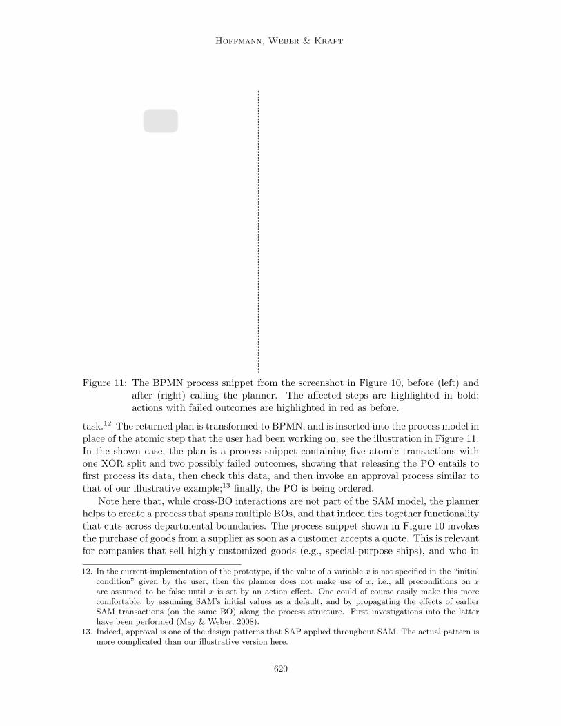
Hoffmann, Weber & Kraft
Notification:
Quote
rejected
Notification:
Quote
accepted
Mark Customer
Quote as
Rejected
Cancel Purchase
Order (2)
Create Sales
Order from
Quote and
archive Quote
Release
Purchase
Order
Trigger Follow-
up SO processing
Timeout
End
Notification:
Quote
rejected
Notification:
Quote
accepted
Mark Customer
Quote as
Rejected
Cancel Purchase
Order (2)
Trigger Follow-
up SO processing
Timeout
End
Create Sales
Order from
Quote and
archive Quote
Process
Purchase Order
Data
Check Purchase
Order Data
Check Purchase
Order Approval
Status
Decide Purchase
Order Approval
Place Purchase
Order
PO Approval
Not Necessary
PO Approval Necessary
Figure 11: The BPMN process snippet from the screenshot in Figure 10, before (left) andafter (right) calling the planner. The affected steps are highlighted in bold;actions with failed outcomes are highlighted in red as before.
task.12 The returned plan is transformed to BPMN, and is inserted into the process model inplace of the atomic step that the user had been working on; see the illustration in Figure 11.In the shown case, the plan is a process snippet containing five atomic transactions withone XOR split and two possibly failed outcomes, showing that releasing the PO entails tofirst process its data, then check this data, and then invoke an approval process similar tothat of our illustrative example;13 finally, the PO is being ordered.
Note here that, while cross-BO interactions are not part of the SAM model, the plannerhelps to create a process that spans multiple BOs, and that indeed ties together functionalitythat cuts across departmental boundaries. The process snippet shown in Figure 10 invokesthe purchase of goods from a supplier as soon as a customer accepts a quote. This is relevantfor companies that sell highly customized goods (e.g., special-purpose ships), and who in
12. In the current implementation of the prototype, if the value of a variable x is not specified in the “initialcondition” given by the user, then the planner does not make use of x, i.e., all preconditions on x
are assumed to be false until x is set by an action effect. One could of course easily make this morecomfortable, by assuming SAM’s initial values as a default, and by propagating the effects of earlierSAM transactions (on the same BO) along the process structure. First investigations into the latterhave been performed (May & Weber, 2008).
13. Indeed, approval is one of the design patterns that SAP applied throughout SAM. The actual pattern ismore complicated than our illustrative version here.
620

SAP Speaks PDDL
turn must procure customized parts from their suppliers (e.g., ship engines). Such processingrequires to combine services from BOs belonging to Customer Relationship Management(CRM) and Supplier Relationship Management (SRM), and hence from the two “oppositeends” of the system (and company). The designer of the process will typically be intimatelyfamiliar with only one of these two, making it especially helpful to be able to call the plannerto obtain information about the other one.
7.4 Evaluation of our Prototype at SAP
Our prototype was part of a research transfer project with the NetWeaver BPM group,and shaped during several feedback rounds with developers and architects. The evaluationwithin SAP consisted mainly of prototype demonstrations at various SAP events. Forexample, an early version of the tool was demonstrated at the 2008 global meeting of SAPResearch “BPM and SI” (SI stands for “Semantic Integration”), which included participantsfrom SAP partners and development. The demonstrations received positive feedback fromSAP software architects. The perception was that this functionality would significantlystrengthen the link between SAP BPM and the underlying software infrastructure, makingit much easier to access the services provided in an effective manner. Most critical commentswere focused on some choices in the user interface design, such as “non-logicians will notunderstand the meaning of the NOT symbol”, or “the list of several hundred BOs is toolong for a drop-down box”.
We do not have customer evaluation data, and it is not foreseeable when we (or anyoneelse) will be able to obtain such data. When our first prototype became available, a partnerorganization committed to perform a pilot customer evaluation. That commitment wasretracted in the context of the 2008/2009 financial crisis. Anyway, real customer evaluationdata may be impossible to come by, let alone publish, due to privacy reasons.
There are also some issues arising from the positioning of our prototype inside the SAPsoftware architecture. The NetWeaver process execution engine currently does not connectto the actual IT services that implement SAM’s “actions”. While SAM is in productiveuse within Business ByDesign, NetWeaver BPM is built on a different technology stack. Aconnection could in principle be established relatively easily – after all, service-orientationis intended to do exactly this sort of thing – however this connection has not as yet been onSAP’s agenda, and it involves some SAP-internal political issues. The fact that the maindrivers of the presented technology – the authors of this paper – have left the company inthe meantime does of course not help to remedy this problem.
8. Related Work
The basic idea explored in this paper – using planning systems to help business experts tocome up with processes close to the IT infrastructure – has been around for quite a longtime. For example, it was mentioned more than a decade ago by Jonathan et al. (1999). Itis also discussed in the 2003 roadmap of the PLANET Network of Excellence in AI Planning(Biundo et al., 2003). More recently, Rodriguez-Moreno et al. (2007) implemented the ideain the SHAMASH system. SHAMASH is a knowledge-based BPM tool targeted at helpingwith the engineering and optimization of process models (Aler, Borrajo, Camacho, & Sierra-Alonso, 2002). The tool includes, amongst other things, user-friendly interfaces allowing
621

Hoffmann, Weber & Kraft
users to conveniently annotate processes with rich context information, in particular inthe form of “rules” which roughly correspond to planning actions. These rules (and otherinformation) then form the basis for translation into PDDL, and planning for creation ofnew process models.
The largest body of related work was performed during the last decade under a differentname, semantic web service composition (SWSC), in the context of the Semantic WebCommunity (e.g., Ponnekanti & Fox, 2002; Narayanan & McIlraith, 2002; Srivastava, 2002;Constantinescu, Faltings, & Binder, 2004; Agarwal et al., 2005; Sirin, Parsia, Wu, Hendler,& Nau, 2004; Sirin et al., 2006; Meyer & Weske, 2006; Liu, Ranganathan, & Riabov, 2007).In a nutshell, the idea in SWSC is (1) to annotate web services with some declarativeabstract explanation of their functionality, and (2) to exploit these “semantic” annotationsto automatically combine web services for achieving a more complex functionality. WhileSWSC terminology differs from what we use in this paper, the idea is basically the same(although most SWSC works do not address BPM specifically).
The key distinguishing feature of the present work is our approach to obtaining theplanning input (the “semantic annotations”). Ours is the first attempt to address theplanning/SWSC problem based on SAM, and more generally based on any pre-existingmodel at all. Since modeling is costly (Kambhampati, 2007; Rodriguez-Moreno et al.,2007), this shift of focus gets us around one of the major open problems in the area. Themodeling interfaces in SHAMASH (Rodriguez-Moreno et al., 2007), and some related worksattempting to support model creation (Gonzalez-Ferrer, Fernandez-Olivares, & Castillo,2009; Cresswell, McCluskey, & West, 2009, 2010), address the same problem, but in verydifferent ways and to a less radical extent. Whereas these works attempt to ease themodeling overhead, our re-use of SAM actually removes that overhead completely.
Having said that, of course there are relations between SAM planning and previous work,at the technical level. In particular, the planning and SWSC literature contains a multitudeof works dealing with actions that, like SAM’s disjunctive effect actions, have more than onepossible outcome. Our semantics for such actions, as detailed already in Section 4.2, is astraightforward mixture of two wide-spread notions in planning: observation actions, whereone out of a list of possible observations is distinguished, and non-deterministic actions,where one out of a list of possible effects occurs (e.g., Weld et al., 1998; Smith & Weld,1999; Bonet & Geffner, 2000; Cimatti et al., 2003; Bryce & Kambhampari, 2004; Hoffmann& Brafman, 2005; Bonet & Givan, 2006; Bryce, Kambhampati, & Smith, 2006; Bryce &Buffet, 2008; Palacios & Geffner, 2009).
A prominent line of research in web service composition, known as “the Roman model”(e.g., Berardi, Calvanese, De Giacomo, Lenzerini, & Mecella, 2003, 2005; De Giacomo &Sardina, 2007; Sardina, Patrizi, & De Giacomo, 2008; Calvanese, De Giacomo, Lenzerini,Mecella, & Patrizi, 2008), also deals with a notion of “non-determinism” in the componentweb services, however the framework is very different from ours. The web services in theRoman model are stateful. That is, each service has a set of possible own/internal states,and the service provides a set of operations to the outside world, which are responsible fortransitions in the service’s internal state. The composition task is to create a scheduler (afunction choosing one service for each operation demanded) interacting with the componentservices in a way such that they implement a desired goal transition system. Similarly, theweb service composition techniques developed by Marco Pistore and his co-workers (e.g.,
622

SAP Speaks PDDL
Pistore, Marconi, Bertoli, & Traverso, 2005; Bertoli, Pistore, & Traverso, 2006, 2010) dealwith this form of non-determinism in stateful component services formalized as transitionsystems. In their work, the composition task is to create a controller transition system suchthat the overall (controlled) behavior satisfies a planning-like goal (expressed in the EAGLElanguage, cf. below). In that latter aspect – attempting to satisfy a planning goal – theirframework is slightly closer to ours than the Roman model.
The main distinguishing feature of our formalism is its notion of “weak SAM plans”,allowing failed action outcomes but only if they are proved unsolvable, and only if at leastone outcome of each action is successful. Some other works have also proposed notionsof plans that do not guarantee to achieve the goal in all cases, and some notions of morecomplex goals can be used to achieve similar effects. We now briefly discuss the notionsclosest to our own approach.
The notions of weak and strong plans, as discussed in Section 4.2, were first introduced byCimatti, Giunchiglia, Giunchiglia, and Traverso (1997) and Cimatti, Roveri, and Traverso(1998b), respectively. Strong cyclic plans were first introduced by Cimatti, Roveri, andTraverso (1998a). That notion is orthogonal to weak SAM plans in that neither implies theother. For example, if a “bad” action outcome invalidates, as a side effect, the preconditionsof all actions in the task, then that action may form part of a weak SAM plan, but neverof a strong cyclic plan. Vice versa, strong cyclic plans have a more general structure, inparticular allowing non-deterministic actions to appear more than once in an execution.
Pistore and Traverso (2001) generalize weak, strong, and strong cyclic plans by handlinggoals taking the form of CTL formulas. However, as pointed out by Dal Lago et al. (2002),such goals are unable to express that the plan should try to achieve the goal, and give uponly if that is not possible. Dal Lago et al. design the goal language EAGLE which addresses(amongst others) this shortcoming. EAGLE features a variety of goal operators that canbe flexibly combined to form goal expressions. One such expression is “TryReach G1 FailG2”, where G1 and G2 are alternative goals. The intuition is that the plan should try toachieve G1, and resort to G2 if reaching G1 has become impossible. More precisely, a planT for such an EAGLE goal is optimal if, for every state s it traverses: (1) T is a strong planfor G1 ∨ G2; (2) if there exists a strong plan for G1 from s, then T is such a strong plan;and (3) if there exists a weak plan for G1 from s, then T is such a weak plan. Applying thisto our context, say we restrict plans to execute each non-deterministic action at most once.It is easy to see that, within this space of plans, every weak SAM plan is optimal for theEAGLE goal “TryReach G Fail TRUE”: weak SAM plans mark s as failed only if reachingG from s is impossible. However, not every action tree T that is optimal for “TryReach G
Fail TRUE” is a weak SAM plan. That is because (2) and (3) do not force every actionto have at least one solved outcome. In tasks for which no weak SAM plan exists, anyaction tree (e.g., the empty tree) is optimal for “TryReach G Fail TRUE”. In tasks with aweak SAM plan, “TryReach G Fail TRUE” forces each solvable action outcome to providea solution, but imposes no constraints below failed outcomes (which may thus be continuedby arbitrarily complex sub-plans).
Shaparau et al. (2006) define a framework that has a similar effect in our context. Theyconsider contingent planning in the presence of a linear preference order over alternativegoals. Action trees T are plans if they achieve at least one goal in every leaf, i.e., they arestrong plans for the disjunction of the goals. Plan T is at least as good as plan T ′ if, in every
623

Hoffmann, Weber & Kraft
state common to both, the best possible outcome achievable using T is at least as good asthat achievable using T ′. T is optimal if it is at least as good as all other plans. Giventhis, like for the EAGLE goal “TryReach G Fail TRUE” discussed above, every weak SAMplan is optimal for the goal preference “G, TRUE”, but the inverse is not true because, inunsolvable tasks and below unsolvable outcomes in solvable tasks, “G, TRUE” permits theplan to do anything.
Mediratta and Srivastava (2006) define a framework also based on contingent planning,but where the user provides as additional input a number K. Then, (1) a “plan” is any treeT with ≥ K leaves achieving the goal; and (2) if such T does not exist, then a “plan” is anytree whose number of such leaves is maximal. Due to (1), failed nodes are not necessarilyunsolvable (the plan may simply stop once it reached K). Due to (2), even a task wherethe goal cannot be reached at all, i.e., no matter what the action outcomes are we cannotachieve the goal, has a “plan”. In addition, in our application context there is no sensibleway, for the human modeler, to choose a meaningful value for K.
Summing up, related notions of weak plans exist, but none captures exactly what wewant in SAM. On the algorithmic side, all the works listed here use symbolic search (basedon BDDs), and are thus quite different from our explicit-state SAM-AO* search. The singleexception is the planner described by Mediratta and Srivastava (2006), which is based on avariant of A*, but for a different plan semantics as described.
Research has been performed also into alternative methods, not based on planning, forautomatically generating processes. For example, Kuster, Ryndina, and Gall (2007) describea method computing the synchronized product of the life-cycles of a set of business objects,and generating a process corresponding to that product. That process serves as the basis forcustomer-specific modifications. Clearly, that motivation relates to ours; but the intendedmeaning of the output (the generated process), and the input assumed for its generation,are quite different. As for the input, Kuster et al.’s life-cycles are state machines describingall possible behaviors of the object, which in our formulation here corresponds to the spaceof all reachable states. That space can be generated based on SAM, but it can be huge evenfor single BOs, not to mention their product (cf. our results for blind search and scalingacross BOs, Sections 6.4 and 6.5). Heuristic search gets us around the need to enumerateall these states. As for the output, Kuster et al.’s generated processes guarantee not only tocomply with the BO behaviors (which ours do as well), but also to cover them, essentiallyrepresenting all that could be done. This is very different from the plans we generate,whose intention is to show specifically how to move between particular start and end states.Altogether, the methods are complementary. Planning has computational advantages if theinvolved objects have many possible states, as is often the case in SAM.
9. Conclusion
We have pointed out that SAP has built a large-scale model of software behavior, SAM,whose abstraction level and formalization are intimately related to planning models in lan-guages such as PDDL. We have shown how to base a promising BPM application of planningon this fact. Getting the planner input for free, we avoid one of the most important obstaclesfor making this kind of planning application successful in practice. Our solution is specificto our particular context in its treatment of non-deterministic actions and failed outcomes,
624

SAP Speaks PDDL
but such phenomena are quite common in both planning and web service composition, andour novel approach to dealing with them might turn out to be relevant more generally.
The main open issue is to obtain concrete data evaluating the business value of ourapplication. Some other points are:
• Our modification of FF successfully handles many SAM instances, finding plans withinruntimes small enough to apply realistic online-setting cut-offs. About 15% of theinstances we encountered still present challenges. These instances could serve as aninteresting benchmark for approaches dealing with failed outcomes in ways related towhat we do here (cf. Section 8).
• The current SAM model does not reflect dependencies across BOs. Such dependenciesdo, however, exist in various forms. For example, some BOs form part of the datacontained in another kind of BO, some actions on one kind of BO create a newinstance of another kind of BO, and some actions must be taken by several BOstogether. There is an ongoing activity at SAP Research, aiming at enriching SAM toreflect some of these interactions, with the purpose of more informed model checking.All the interactions can easily be modeled in terms of well-known planning constructs(object creation, and preconditions/effects spanning variables from several BOs), sowe expect that this extended model will enable us to generate more accurate plans. Asthe results from Section 6.5 indicate, additional planning techniques may be requiredto improve performance in case the number of interacting BOs becomes large. Butfor smaller numbers (up to around a dozen BOs) the performance of our current toolshould still be reasonable.
• SAM currently provides no basis for automatically creating a number of additionalprocess aspects. An important aspect is exception handling, for which at the momentwe can only highlight the places (failed nodes) where it needs to be inserted. Anotherissue is data-flow. This is mostly easy since the application data is already pre-packaged in the relevant BOs, but there are some cases, like security tokens, notcovered by this. An open line of research is to determine how these aspects could bemodeled, in a way that can be exploited by corresponding planning algorithms.
• It may also be interesting to look into methods presenting the user with a set ofalternative processes. For discerning between relevant alternatives, such methodsrequire extensions to SAM, like action duration, action cost, or plan preferences.
From a more general perspective, the key contribution of our work is demonstrating thepotential synergy between model-based software engineering and planning-based processgeneration. Re-using some (or even all) of the required models, the human labor requiredto realize the planning is dramatically reduced. SAM’s methodology – business-level de-scriptions of individual activities within a software architecture – is not specific to SAP.Thus, exploiting this synergy is a novel approach that may turn out fruitful far beyond theparticular application described herein.
Acknowledgments
We thank the anonymous JAIR reviewers, whose comments helped a lot in improving thepaper.
625

Hoffmann, Weber & Kraft
Most of this work was performed while all authors were employed by SAP. Part of thiswork was performed while Jorg Hoffmann was employed by INRIA (Nancy, France), andwhile Ingo Weber was employed by The University of New South Wales (Sydney, Australia).
NICTA is funded by the Australian Government as represented by the Department ofBroadband, Communications and the Digital Economy and the Australian Research Councilthrough the ICT Centre of Excellence program.
References
Aalst, W. (1997). Verification of Workflow Nets. In Application and Theory of Petri Nets1997.
Agarwal, V., Chafle, G., Dasgupta, K., Karnik, N., Kumar, A., Mittal, S., & Srivastava, B.(2005). Synthy: A system for end to end composition of web services. Journal of WebSemantics, 3 (4).
Aler, R., Borrajo, D., Camacho, D., & Sierra-Alonso, A. (2002). A knowledge-based ap-proach for business process reengineering: SHAMASH. Knowledge Based Systems,15 (8), 473–483.
Bacchus, F. (2000). Subset of PDDL for the AIPS2000 Planning Competition. The AIPS-00Planning Competition Comitee.
Backstrom, C., & Nebel, B. (1995). Complexity results for SAS+ planning. ComputationalIntelligence, 11 (4), 625–655.
Bell, M. (2008). Service-Oriented Modeling: Service Analysis, Design, and Architecture.Wiley & Sons.
Berardi, D., Calvanese, D., De Giacomo, G., Lenzerini, M., & Mecella, M. (2003). Au-tomatic composition of e-services that export their behavior. In Orlowska, M. E.,Weerawarana, S., Papazoglou, M. P., & Yang, J. (Eds.), Proceedings of the 1st Inter-national Conference on Service-Oriented Computing (ICSOC’03), Vol. 2910 of LectureNotes in Computer Science, pp. 43–58. Springer.
Berardi, D., Calvanese, D., De Giacomo, G., Lenzerini, M., & Mecella, M. (2005). Auto-matic service composition based on behavioral descriptions. International Journal ofCooperative Information Systems, 14 (4), 333–376.
Bertoli, P., Pistore, M., & Traverso, P. (2006). Automated web service composition byon-the-fly belief space search. In Long, D., & Smith, S. (Eds.), Proceedings of the16th International Conference on Automated Planning and Scheduling (ICAPS-06),Ambleside, UK. AAAI.
Bertoli, P., Pistore, M., & Traverso, P. (2010). Automated composition of web services viaplanning in asynchronous domains. Artificial Intelligence, 174 (3-4), 316–361.
Biundo, S., Aylett, R., Beetz, M., Borrajo, D., Cesta, A., Grant, T., McCluskey, L., Milani,A., & Verfaillie, G. (2003). PLANET Technological Roadmap on AI Planning andScheduling. http://planet.dfki.de/service/Resources/Roadmap/Roadmap2.pdf.
Bonet, B., & Geffner, H. (2000). Planning with incomplete information as heuristic search inbelief space. In Chien, S., Kambhampati, R., & Knoblock, C. (Eds.), Proceedings of the
626

SAP Speaks PDDL
5th International Conference on Artificial Intelligence Planning Systems (AIPS-00),pp. 52–61, Breckenridge, CO. AAAI Press, Menlo Park.
Bonet, B., & Geffner, H. (2001). Planning as heuristic search. Artificial Intelligence, 129 (1–2), 5–33.
Bonet, B., & Givan, B. (2006). 5th international planning competition: Non-deterministictrack – call for participation. In Proceedings of the 5th International Planning Com-petition (IPC’06).
Born, M., Hoffmann, J., Kaczmarek, T., Kowalkiewicz, M., Markovic, I., Scicluna, J., Weber,I., & Zhou, X. (2008). Semantic annotation and composition of business processes withMaestro. In Demonstrations at ESWC’08: 5th European Semantic Web Conference,pp. 772–776, Tenerife, Spain.
Born, M., Hoffmann, J., Kaczmarek, T., Kowalkiewicz, M., Markovic, I., Scicluna, J., We-ber, I., & Zhou, X. (2009). Supporting execution-level business process modelingwith semantic technologies. In Demonstrations at DASFAA’09: Database Systems forAdvanced Applications, pp. 759–763, Brisbane, Australia.
Bryce, D., & Buffet, O. (2008). 6th international planning competition: Uncertainty part.In Proceedings of the 6th International Planning Competition (IPC’08).
Bryce, D., & Kambhampari, S. (2004). Heuristic guidance measures for conformant plan-ning. In Koenig, S., Zilberstein, S., & Koehler, J. (Eds.), Proceedings of the 14thInternational Conference on Automated Planning and Scheduling (ICAPS-04), pp.365–374, Whistler, Canada. AAAI.
Bryce, D., Kambhampati, S., & Smith, D. E. (2006). Planning graph heuristics for beliefspace search. Journal of Artificial Intelligence Research, 26, 35–99.
Bylander, T. (1994). The computational complexity of propositional STRIPS planning.Artificial Intelligence, 69 (1–2), 165–204.
Calvanese, D., De Giacomo, G., Lenzerini, M., Mecella, M., & Patrizi, F. (2008). Automaticservice composition and synthesis: the roman model. IEEE Data Engineering Bulletin,31 (3), 18–22.
Cimatti, A., Giunchiglia, F., Giunchiglia, E., & Traverso, P. (1997). Planning via modelchecking: A decision procedure for ar. In Steel, S., & Alami, R. (Eds.), Recent Advancesin AI Planning. 4th European Conference on Planning (ECP’97), Vol. 1348 of LectureNotes in Artificial Intelligence, pp. 130–142, Toulouse, France. Springer-Verlag.
Cimatti, A., Pistore, M., Roveri, M., & Traverso, P. (2003). Weak, strong, and strong cyclicplanning via symbolic model checking. Artificial Intelligence, 147 (1-2), 35–84.
Cimatti, A., Roveri, M., & Traverso, P. (1998a). Automatic obdd-based generation ofuniversal plans in non-deterministic domains. In Mostow, J., & Rich, C. (Eds.),Proceedings of the 15th National Conference of the American Association for ArtificialIntelligence (AAAI-98), pp. 875–881, Madison, WI, USA. MIT Press.
Cimatti, A., Roveri, M., & Traverso, P. (1998b). Strong planning in non-deterministic do-mains via model checking. In Simmons, R., Veloso, M., & Smith, S. (Eds.), Proceed-ings of the 4th International Conference on Artificial Intelligence Planning Systems(AIPS-98), pp. 36–43, Pittsburgh, PA. AAAI Press, Menlo Park.
627

Hoffmann, Weber & Kraft
Cohn, D., & Hull, R. (2009). Business artifacts: A data-centric approach to modelingbusiness operations and processes. IEEE Data Engineering Bulletin, 3–9.
Constantinescu, I., Faltings, B., & Binder, W. (2004). Large scale, type-compatible servicecomposition. In Jain, H., & Liu, L. (Eds.), Proceedings of the 2nd InternationalConference on Web Services (ICWS-04), pp. 506–513, San Diego, California, USA.IEEE Computer Society.
Cresswell, S., McCluskey, T., & West, M. (2010). Acquiring planning domains models usingLOCM. The Knowledge Engineering Review.
Cresswell, S., McCluskey, T. L., & West, M. M. (2009). Acquisition of object-centred domainmodels from planning examples. In Gerevini, A., Howe, A. E., Cesta, A., & Refanidis,I. (Eds.), Proceedings of the 19th International Conference on Automated Planningand Scheduling (ICAPS-09), Sydney, Australia. AAAI.
Dal Lago, U., Pistore, M., & Traverso, P. (2002). Planning with a language for extendedgoals. In Dechter, R., Kearns, M., & Sutton, R. (Eds.), Proceedings of the 18th NationalConference of the American Association for Artificial Intelligence (AAAI-02), pp.447–454, Edmonton, AL, USA. MIT Press.
De Giacomo, G., & Sardina, S. (2007). Automatic synthesis of new behaviors from a libraryof available behaviors. In Veloso, M. (Ed.), Proceedings of the 20th International JointConference on Artificial Intelligence (IJCAI-07), pp. 1866–1871, Hyderabad, India.Morgan Kaufmann.
Dumas, M., ter Hofstede, A., & van der Aalst, W. (Eds.). (2005). Process Aware Infor-mation Systems: Bridging People and Software Through Process Technology. WileyPublishing.
Fox, M., & Long, D. (2003). PDDL2.1: An extension to PDDL for expressing temporalplanning domains. Journal of Artificial Intelligence Research, 20, 61–124.
Gazen, B. C., & Knoblock, C. (1997). Combining the expressiveness of UCPOP withthe efficiency of Graphplan. In Steel, S., & Alami, R. (Eds.), Recent Advances inAI Planning. 4th European Conference on Planning (ECP’97), Vol. 1348 of LectureNotes in Artificial Intelligence, pp. 221–233, Toulouse, France. Springer-Verlag.
Gerevini, A., Haslum, P., Long, D., Saetti, A., & Dimopoulos, Y. (2009). Deterministicplanning in the fifth international planning competition: PDDL3 and experimentalevaluation of the planners. Artificial Intelligence, 173 (5-6), 619–668.
Gonzalez-Ferrer, A., Fernandez-Olivares, J., & Castillo, L. (2009). JABBAH: a Java ap-plication framework for the translation between business process models and HTN.In Proceedings of the 3rd International Competition on Knowledge Engineering forPlanning and Scheduling, Thessaloniki, Greece.
Helmert, M. (2006). The Fast Downward planning system. Journal of Artificial IntelligenceResearch, 26, 191–246.
Helmert, M. (2009). Concise finite-domain representations for pddl planning tasks. ArtificialIntelligence, 173 (5-6), 503–535.
628

SAP Speaks PDDL
Hoffmann, J., & Brafman, R. (2005). Contingent planning via heuristic forward search withimplicit belief states. In Biundo, S., Myers, K., & Rajan, K. (Eds.), Proceedings of the15th International Conference on Automated Planning and Scheduling (ICAPS-05),pp. 71–80, Monterey, CA, USA. AAAI.
Hoffmann, J., & Edelkamp, S. (2005). The deterministic part of IPC-4: An overview. Journalof Artificial Intelligence Research, 24, 519–579.
Hoffmann, J., & Nebel, B. (2001). The FF planning system: Fast plan generation throughheuristic search. Journal of Artificial Intelligence Research, 14, 253–302.
Jonathan, P. J., Moore, J., Stader, J., Macintosh, A., & Chung, P. (1999). Exploiting aitechnologies to realise adaptive workflow systems. In Proceedings ot the AAAI’99Workshop on Agent-Based Systems in the Business Context.
Kambhampati, S. (2007). Model-lite planning for the web age masses: The challenges ofplanning with incomplete and evolving domain models. In Howe, A., & Holte, R. C.(Eds.), Proceedings of the 22nd National Conference of the American Association forArtificial Intelligence (AAAI-07), Vancouver, BC, Canada. MIT Press.
Kitchin, D. E., McCluskey, T. L., & West, M. M. (2005). B vs ocl: Comparing specifica-tion languages for planning domains. In Proceedings of the ICAPS’05 Workshop onVerification and Validation of Model-Based Planning and Scheduling Systems.
Krafzig, D., Banke, K., & Slama, D. (2005). Enterprise SOA: Service-Oriented ArchitectureBest Practices. Prentice Hall.
Kuster, J. M., Ryndina, K., & Gall, H. (2007). Generation of business process modelsfor object life cycle compliance. In Alonso, G., Dadam, P., & Rosemann, M. (Eds.),Proceedings of the 5th International Conference on Business Process Management(BPM’07), Vol. 4714 of Lecture Notes in Computer Science, pp. 165–181. Springer.
Liu, Z., Ranganathan, A., & Riabov, A. (2007). A planning approach for message-orientedsemantic web service composition. In Howe, A., & Holte, R. C. (Eds.), Proceedings ofthe 22nd National Conference of the American Association for Artificial Intelligence(AAAI-07), Vancouver, BC, Canada. MIT Press.
May, N., & Weber, I. (2008). Information gathering for semantic service discovery andcomposition in business process modeling. In CIAO!’08: Workshop on Cooperation &Interoperability - Architecture & Ontology at CAiSE’08, Vol. LNBIP 10, pp. 46–60,Montpellier, France.
McDermott, D., Ghallab, M., Howe, A., Knoblock, C., Ram, A., Veloso, M., Weld, D., &Wilkins, D. (1998). PDDL – the planning domain definition language. Tech. rep.CVC TR-98-003, Yale Center for Computational Vision and Control.
McDermott, D. V. (1999). Using regression-match graphs to control search in planning.Artificial Intelligence, 109 (1-2), 111–159.
Mediratta, A., & Srivastava, B. (2006). Applying planning in composition of web serviceswith a user-driven contingent planner. IBM Research Report RI 06002.
Meyer, H., & Weske, M. (2006). Automated service composition using heuristic search. InDustdar, S., Fiadeiro, J. L., & Sheth, A. P. (Eds.), Proceedings of the 4th International
629

Hoffmann, Weber & Kraft
Conference on Business Process Management (BPM’06), Vol. 4102 of Lecture Notesin Computer Science, pp. 81–96. Springer.
Narayanan, S., & McIlraith, S. (2002). Simulation, verification and automated compositionof web services. In Iyengar, A., & Roure, D. D. (Eds.), Proceedings of the 11th Inter-national World Wide Web Conference (WWW-02), Honolulu, Hawaii, USA. ACM.
Nilsson, N. J. (1969). Searching problem-solving and game-playing trees for minimal costsolutions. In Information Processing 68 Vol. 2, pp. 1556–1562, Amsterdam, Nether-lands.
Nilsson, N. J. (1971). Problem Solving Methods in Artificial Intelligence. McGraw-Hill.
Object Management Group (2006). Object Constraint Language Specification, Version 2.http://www.omg.org/technology/documents/formal/ocl.htm.
Object Management Group (2008). Business Process Modeling Notation, V1.1.http://www.bpmn.org/.
Palacios, H., & Geffner, H. (2009). Compiling uncertainty away in conformant planningproblems with bounded width. Journal of Artificial Intelligence Research, 35, 623–675.
Pearl, J. (1984). Heuristics. Morgan Kaufmann.
Pednault, E. P. (1989). ADL: Exploring the middle ground between STRIPS and the situ-ation calculus. In Brachman, R., Levesque, H. J., & Reiter, R. (Eds.), Principles ofKnowledge Representation and Reasoning: Proceedings of the 1st International Con-ference (KR-89), pp. 324–331, Toronto, ON. Morgan Kaufmann.
Pesic, M., Schonenberg, M. H., Sidorova, N., & van der Aalst, W. M. P. (2007). Constraint-based workflow models: Change made easy. In Meersman, R., & Tari, Z. (Eds.), OTMConferences (1), Vol. 4803 of Lecture Notes in Computer Science, pp. 77–94. Springer.
Pistore, M., Marconi, A., Bertoli, P., & Traverso, P. (2005). Automated composition of webservices by planning at the knowledge level. In Kaelbling, L. (Ed.), Proceedings of the19th International Joint Conference on Artificial Intelligence (IJCAI-05), Edinburgh,Scotland. Morgan Kaufmann.
Pistore, M., & Traverso, P. (2001). Planning as model checking for extended goals in non-deterministic domains. In Nebel, B. (Ed.), Proceedings of the 17th International JointConference on Artificial Intelligence (IJCAI-01), pp. 479–486, Seattle, Washington,USA. Morgan Kaufmann.
Ponnekanti, S., & Fox, A. (2002). SWORD: A developer toolkit for web services composition.In Iyengar, A., & Roure, D. D. (Eds.), Proceedings of the 11th International WorldWide Web Conference (WWW-02), Honolulu, Hawaii, USA. ACM.
Richter, S., & Helmert, M. (2009). Preferred operators and deferred evaluation in satisficingplanning. In Gerevini, A., Howe, A. E., Cesta, A., & Refanidis, I. (Eds.), Proceedingsof the 19th International Conference on Automated Planning and Scheduling (ICAPS-09), Sydney, Australia. AAAI.
Rodriguez-Moreno, M. D., Borrajo, D., Cesta, A., & Oddi, A. (2007). Integrating planningand scheduling in workflow domains. Expert Systems Applications, 33 (2), 389–406.
630
SAP Speaks PDDL
SAP (2010). SAP NetWeaver.. http://www.sap.com/platform/netweaver/index.epx.
Sardina, S., Patrizi, F., & De Giacomo, G. (2008). Behavior composition in the presenceof failure. In Brewka, G., & Lang, J. (Eds.), Proceedings of the 11th InternationalConference on Principles of Knowledge Representation and Reasoning (KR’08), pp.640–650. AAAI Press.
Schneider, S. (2001). The B-Method: An Introduction. Palgrave.
Shaparau, D., Pistore, M., & Traverso, P. (2006). Contingent planning with goal preferences.In Gil, Y., & Mooney, R. J. (Eds.), Proceedings of the 21st National Conference of theAmerican Association for Artificial Intelligence (AAAI-06), Boston, Massachusetts,USA. MIT Press.
Sirin, E., Parsia, B., Wu, D., Hendler, J., & Nau, D. (2004). HTN planning for web servicecomposition using SHOP2. Journal of Web Semantics, 1 (4).
Sirin, E., Parsia, B., & Hendler, J. (2006). Template-based composition of semantic webservices. In AAAI Fall Symposium on Agents and Search.
Smith, D. E., & Weld, D. S. (1999). Temporal planning with mutual exclusion reasoning. InDean, T. (Ed.), Proceedings of the 16th International Joint Conference on ArtificialIntelligence (IJCAI-99), pp. 326–337, Stockholm, Sweden. Morgan Kaufmann.
Srivastava, B. (2002). Automatic web services composition using planning. In KnowledgeBased Computer Systems (KBCS-02), pp. 467–477.
Traverso, P., Ghallab, M., & Nau, D. (Eds.). (2005). Automated Planning: Theory andPractice. Morgan Kaufmann.
Turner, J., & McCluskey, T. L. (1994). The Construction of Formal Specifications: anIntroduction to the Model-Based and Algebraic Approaches. McGraw Hill SoftwareEngineering series.
van der Aalst, W. (2003). Business process management demystified: A tutorial on models,systems and standards for workflow management. In Lectures on Concurrency andPetri Nets in ACPN’04: Advanced Courses in Petri Nets, pp. 1–65.
van der Aalst, W. M. P., & Pesic, M. (2006). Decserflow: Towards a truly declarative serviceflow language. In Bravetti, M., Nunez, M., & Zavattaro, G. (Eds.), WS-FM, Vol. 4184of Lecture Notes in Computer Science, pp. 1–23. Springer.
Wainer, J., & de Lima Bezerra, F. (2003). Groupware: Design, Implementation, and Use,Vol. 2806 of LNCS, chap. Constraint-based flexible workflows, pp. 151–158. Springer-Verlag.
Weld, D. S., Anderson, C. R., & Smith, D. E. (1998). Extending graphplan to handleuncertainty & sensing actions. In Mostow, J., & Rich, C. (Eds.), Proceedings ofthe 15th National Conference of the American Association for Artificial Intelligence(AAAI-98), pp. 897–904, Madison, WI, USA. MIT Press.
Weske, M. (2007). Business Process Management: Concepts, Languages, Architectures.Springer-Verlag.
631

Hoffmann, Weber & Kraft
Yoon, S. W., Fern, A., & Givan, R. (2007). FF-Replan: A baseline for probabilistic planning.In Boddy, M., Fox, M., & Thiebaux, S. (Eds.), Proceedings of the 17th InternationalConference on Automated Planning and Scheduling (ICAPS-07), Providence, RhodeIsland, USA. AAAI.
Younes, H., Littman, M., Weissman, D., & Asmuth, J. (2005). The first probabilistic trackof the international planning competition. Journal of Artificial Intelligence Research,24, 851–887.
632