san francisco bay nutrient management strategy science plan · san francisco bay nutrient...
TRANSCRIPT

1
San Francisco Bay
Nutrient Management Strategy
Science Plan
March 15 2016

2
1. Introduction The San Francisco Bay (SFB) estuary receives large inputs of the nutrients nitrogen and
phosphorous from anthropogenic sources, and has the potential to suffer negative impacts from
nutrient overenrichment. Nutrient concentrations in SFB exceed those in other estuarine
ecosystems where degradation is strongly expressed. To date, SFB has shown resistance to some
of the classic symptoms of nutrient over-enrichment, such as excessive phytoplankton biomass
as chlorophyll-a (chl-a) and low dissolved oxygen (DO). Recent observations, however, suggest
that SFB’s resistance to nutrient enrichment is weakening, and have generated concern that SFB
may be trending toward, or may already be experiencing, adverse impacts due to its high nutrient
loads. In response to these concerns, the San Francisco Bay Regional Water Quality Control
Board (SFBRWQCB) worked collaboratively with stakeholders to develop the San Francisco
Bay Nutrient Management Strategy (NMS).1 The NMS lays out an overall approach for
developing the underlying science to support nutrient management decisions.
This report presents a Draft Science Plan for implementing the SFB NMS. The report’s main
goals include:
1. Lay out a multi-year Science Plan representing a logical sequence of studies to inform
major management decisions, assuming a time-line of 10+ years.
2. Develop an approach and rationale for sequencing and prioritizing among studies, and
identify specific high-priority studies, in particular those that should proceed in FY2016-
2018.
3. Provide realistic estimates of the time-frame and funding needed to support a Science
Plan that will successfully inform management decisions.
The Draft Science Plan was developed in 2014-15 with input from science advisors (Table 1.1),
the NMS Steering Committee, and the NMS Nutrient Technical Work Group (Fig. 1.1). Projects
are described in more detail in the first 1-3 years, and in increasingly less detail over time,
recognizing that the Science Plan will be iteratively refined based on new insights gained as
work progresses.
Table 1.1 Science Advisors for NMS Science Plan
James Cloern, PhD USGS Lawrence Harding, PhD UCLA Wim Kimmerer, PhD SFSU-RTC Raphael Kudela, PhD UC Santa Cruz Mark Stacey, PhD UC Berkeley Martha Sutula, PhD SCCWRP
The science advisor team was convened in December 2014 to provide initial input on the Science
Plan, discuss priorities for specific studies, and recommend a sequence and time-line to address
1http://www.waterboards.ca.gov/sanfranciscobay/water_issues/programs/planningtmdls/amendments/estuarineNNE/Nutrient_Strategy%20November%202012.pdf

3
management questions. During two meetings (October 2014, February 2014), the NMS Steering
Committee provided guidance on the approach for developing the Science Plan and science and
management priorities. The Nutrient Technical Workgroup also provided input during a meeting
in April 2014. Additional science advisor meeting is planned for Summer/Fall 2015 to help
develop the plan’s final draft, and provide input on specific projects for FY2016.
The Draft Science Plan is described in Section 2 and Appendix 1. Relevant background
information on nutrient issues in San Francisco Bay, and a summary of major science needs and
recommended priorities, are presented in Appendix 2-4 (Section 4). The background material
and recommendations were originally presented in an earlier report (Scientific Foundation for the
San Francisco Bay Nutrient Management Strategy; SFEI 2014).
Figure 1.1 Proposed process and timeline for Science Plan development. Actual dates differ from those depicted. A draft Science Plan was used to guide FY16 funding decision in June 2015. Stakeholder comments were received in June/July 2015, and comments from two external peer reviewers in March 2016 (see Appendix 5). An External Science Panel Review will occur sometime in FY17 or later.
link
link
link
link
link
link
link
link

4
2. Science Plan
2.1 Management Questions and Knowledge / Data Gaps The Science Plan aims to build the scientific foundation needed by regulators and stakeholders to answer the six management questions in Table 2.1. High priority knowledge and data gaps related to nutrient loads, nutrient cycling and ecosystem response to nutrients in SFB were identified in SFEI (2014), and are summarized in Appendix 4.
Table 2.1 Management questions targeted by the NMS Science Plan
1. What conditions in different SFB habitats would indicate that beneficial uses are being protected versus experiencing nutrient-related impairment?
2. In which subembayments or habitats are beneficial uses being supported? Which subembayments or habitats are experiencing nutrient-related impairment?
3.a To what extent is nutrient over-enrichment, versus other factors, responsible for current impairments?
3.b What management actions would be required to mitigate those impairments and protect beneficial uses?
4.a Under what future scenarios could nutrient-related impairments occur, and which of these scenarios warrant pre-emptive management actions?
4.b What management actions would be required to protect beneficial uses under those scenarios?
5. What nutrient sources contribute to elevated nutrient concentrations in SFB subembayments or habitats that are currently impaired, or would be impaired in the future, by nutrients?
6. When nutrients exit SFB through the Golden Gate, where are they transported and how do they influence water quality in the Gulf of Farallones or other coastal areas?
7. What specific management actions, including load reductions, are needed to mitigate or prevent current or future impairment?

5
2.2 Science Plan Structure Activities in the Science Plan are organized by Major Program Areas and Work Categories (Table 2.3), based on the priority science needs detailed in Appendix 4 and in SFEI (2014). Program Areas 2, 3, and 4 address the five pathways for adverse impacts presented in Figure A.3.1. Program Area 1, Nutrients, is presented as a separate Program Area because defining the sources, fate, and transport of nutrients is essential to all elements of the Science Plan. Activities in each of the first four program areas are divided into 5 Work Categories (Table 2.3). Note that three Work Categories also appear as sub-headings under Program Area 5, Program-wide Activities. Monitoring, Modeling, and Protective Conditions / Asssessement Framework are essential components of Program Areas 1-4, but are also themselves major programmatic undertakings, with technical activities and coordination that are not well-placed under Program Areas 1-4. Table 2.2 Science Plan structure
Major Program Areas Work Categories
1. Nutrients (loads, cycling/transformations)
A. Synthesis
B. Monitoring
C. Special Studies
D. Modeling (current conditions)
F. Identify Protective Conditions
F. Modeling condition under plausible future scenarios
2. High biomass and low dissolved oxygen
2.1 Deep subtidal
2.2 Shallow margin habitats
3. Phytoplankton community composition
3.1 HABs/toxins
3.2 Food quality (due to N:P, NH4, etc.)
4. Low productivity
5. Program-wide Activities
5.1 Monitoring Future monitoring program design, including considerations of science requirements, logistics, institutional agreements, and funding
5.2 Modeling Base model development, model documentation, model maintenance
5.3 Protective Conditions/Assessment Framework Iteratively refine framework based on new data.
5.4 Program Management Science communication, stakeholder engagement, coordination among projects, fundraising

6
Table 2.3 Work Categories within the Major Program Areas
Work Categories Types of activities
A. Synthesis
Analyzing/synthesizing new results from past studies, developing conceptual models, etc., to identify science needs
Analyzing/synthesizing new data from monitoring and special studies to inform next steps in science plan implementation
Workshops to identify highest priority science questions and experiments
B. Monitoring
Current ship-based monitoring, Bay-wide…nutrients, phytoplankton biomass, phytoplankton composition, physical observations (salinity, temperature, SPM, etc.)
Moored sensors…biogeochemical data, physical data (T, salinity, stratification, velocities, etc.)
Future monitoring program design: data analysis and expert input on spatial/temporal resolution, blend of ship-based vs. fixed-station continuous monitoring, new measurements, etc.
C. Special Studies
Field investigations to o measure biogeochemical processes: e.g., primary production,
nutrient transformations (water column, benthic), DO consumption (water column, benthic)
o collect physical observations (T, sal, velocities, light levels) to quantify mixing, transport, and stratification
o study processes or test hypotheses at the ecosystem-scale (e.g., factors that influence HABs or toxin production)
Mechanistic studies in the laboratory Pilot studies related to monitoring program development, including data
analysis
D. Modeling
Biogeochemical (Water Quality) and hydrodynamic model development and application to quantitatively explore: o Transport of nutrients and biomass o Growth of phytoplankton, grazing by pelagic and benthic grazers,
growth of different types of phytoplankton o Nutrient and organic matter biogeochemical transformations and
losses o Hydrodynamics, effect of physics (e.g., stratification) on env’l
processes
E. Identify Protective Conditions
Levels of DO, chl, and toxins, or characteristics of phytoplankton assemblages that are protective of beneficial uses
Identify the beneficial uses potentially impacted by nutrients. In the case of aquatic life uses, specifically identify the organisms to be protected.
Literature review to identify these levels, modeling (trophic transfer, HAB or toxin bloom size)
Nutrients, loads or concentrations that will protect beneficial uses.
F. Future scenarios Identify high priority environmental change scenarios to test Identify load reduction or management scenarios. Simulate ecosystem response under future scenarios

7
2.3 Timeline and Budget Assumptions In addition to the management questions and science needs, two practical constraints strongly influence the NMS Science Plan’s structure and activities. The first is the proposed timeline for answering management questions. The second is the available funding to support science activities. Currently, both the Science Plan’s timeline and its funding are uncertain. It was not possible to develop the Science Plan with the timeline and budget left fluid; therefore, two major assumptions were made. First, a 10-year time horizon was identified as the goal for reaching sufficiently-confident answers to NMS management questions (Table 2.1). This 10-year time horizon, beginning in July 2014, was based on guidance from the SFBRWQCB. Tables 2.4 and 2.5 present approximate timelines for addressing the management questions in Table 1.1. Table 2.5 organizes management questions into specific questions based on the Major Work Areas in Table 2.2. The sequencing and timeline of Science Plan activities were designed to yield early provisional answers to management questions, and to refine those answers through further investigations that target major uncertainties. This iterative approach allows the Science Plan to be periodically refocused on the highest priority science needs. It would also help identify the need for any early management actions, e.g., if impairment becomes evident. The milestones and dates in Tables 2.4 and 2.5 are realistic in terms of the effort and time required to conduct investigations related to a particular line of inquiry. It is important to note, though, that the schedule assumes that all work proceeds in parallel Second, with the timeline fixed, the Draft Science Plan budget was allowed to expand to match the proposed schedule. As with the schedule, the estimated funding needed to conduct a set of investigations are realistic. However, it became apparent early in Science Plan discussions that the current funding level ($1.38mill/yr) will be insufficient to address all the management questions (Table 2.1) for all potential adverse-impacts pathways (Figure A.3.1) at this pace, given the knowledge and data gaps that need to be addressed (Appendix 4). In addition, some amount of ramp-up time is needed to build a sustainable program. It should be noted that even with an “unlimited resources” approach, some questions remain unanswered at a final level of confidence in a 10-year period. The Draft Science Plan in its current form is thus best considered as an idealized plan – technically feasible but unlikely to proceed as laid out because of funding constraints, and requiring either substantially increased funding or tough decisions about what lines of inquiry and types of investigations are most essential. A process or structure for prioritizing science activities has not yet been developed, and is a necessary upcoming step.

8
T
ab
le 2
.4 M
anag
emen
t q
ues
tio
ns
and
ap
pro
xim
ate
tim
elin
e fo
r it
erat
ivel
y r
each
ing
answ
ers.
Th
e 1
0-y
ear
tim
elin
e is
bas
ed o
n a
Reg
ion
al
Wat
er B
oar
d g
oal
of
esta
bli
shin
g n
utr
ien
t o
bje
ctiv
es f
or
SFB
by
the
end
of
the
seco
nd
Bay
-wid
e n
utr
ien
t p
erm
it (
20
24
). S
ee T
able
2.5
fo
r m
ore
det
aile
d v
ersi
on

9
Ta
ble
2.5
Exp
and
ed v
ersi
on
of
Tab
le 2
.5 d
epic
tin
g sc
hed
ule
of
iter
ativ
ely
an
swer
ing
man
agem
ent
qu
esti
on
s fo
r th
e ra
nge
o
f p
ote
nti
al a
dve
rse
imp
act
pat
hw
ays
and
nu
trie
nt
load
s/tr
ansf
orm
atio
ns.

10
2.4 Regulator and Stakeholder Priorities Input was solicited from regulators, stakeholders, and the NMS Steering Committee at several points during the Science Plan development process to identify priorities and time-sensitive issues. Several themes emerged during these discussions and have been incorporated, to the extent possible, in this version:
1. The Science Plan must consider, and help define, the specific beneficial uses that are targeted for protection, including identifying the organisms and ecosystem services that management actions would aim to protect from nutrient-related adverse impacts.
2. Conditions protective of beneficial uses should be quantitatively identified: e.g., protective DO conditions for specific fish species; protective algal toxins concentrations for chronically-exposed marine biota.
3. Provisional answers to some questions are needed by June 2018 to inform permit renewal discussions:
a. Source-attribution for nutrients in SFB as a function of space and time; b. Define regional demarcations / boundaries in SFB based on retrospective
data analysis of relevant water-quality properties and modeling of sources; c. Initial indications of whether SFB is experiencing nutrient-related adverse
impacts.
4. The Science Plan’s implementation needs a process for prioritizing among science activities (Figure A.3.1) and assessing timeline/schedules, in order to achieve an appropriate balance between program cost, program duration, and the level of confidence in the answers to management questions.
2.5 Rationale/Criteria for Establishing Workflow and Priorities This section provides an overview of several criteria used to guide the development of the Science Plan using the structural elements defined in Tables 2.2 and 2.3. 1. Adopt an approach that produces early guidance, pursues studies to test priority knowledge gaps, and periodically refines guidance based on new information.
Goals: - A Science Plan that targets the highest priority studies, with the expectation that
priorities will evolve based on results from on-going work. - Provisional answers to management questions that can help inform any early
decisions or planning. Build flexibility into the process through planned reassessments (e.g., 3 year cycles): - Periodically revisit the Science Plan, and refine priorities based on new data. - Refine earlier guidance, as necessary, based on new scientific information and
their management implications.

11
2. To the extent possible, use a tiered approach to guide the sequencing or prioritization of projects. This is especially important in the first few years when a major focus needs to be on identifying which pathways (Figure A.3.1) and habitats are most concerning.
The decision tree below illustrates a generalized workflow, organized into tiers. Following this logic, some of the more challenging, costly, and multi-year studies (Tiers 4, 5: e.g., quantitative/mechanistic studies to explore nutrient-HAB linkages; habitat field surveys to characterize DO tolerance) are pursued only after a problem has been identified and a causal link with nutrients established (Tiers 1, 2, 3). Table A.1 serves as an example of sequenced or tiered studies for exploring issues related to HABs/toxins.
Work cannot always strictly follow such a tiered sequence. One example is the coupled hydrodynamic-biogeochemical modeling for SFB, which will take considerable time to develop. Work on model development needs to begin early, unlike what might be suggested by a strictly tiered approach.

12
3. When possible, pursue projects that benefit more than one Program Area, and look for opportunities to leverage efforts in one program area to advance others.
HABs exemplify an undesirable shift of phytoplankton species composition to a community including toxic forms. HAB-related studies (e.g., field investigations using microscopy, pigments, or genomic approaches) will also advance our understanding of factors that shape phytoplankton community composition and food quality more broadly.
Many of the projects identified below have direct and indirect benefits for multiple program areas.
4. Organize field investigations spatially to ensure integrated and efficient collection of necessary data
A diverse array of environmental data is needed to shed light on how SFB responds now to nutrient over-enrichment, and how it may respond in the future.
These data are best collected simultaneously, both to aid in interpretations and
maximize cost-effectiveness (i.e., relatively small incremental cost of adding measurements to a field program than launching a new study)
5. Target high-priority conceptual and data gaps through specific projects in FY2016-FY2018.
Since nutrients have only emerged as a concerning issue in SFB recently, there are many priority needs, including (see also Section A.4.2 and Tables A.4.1-A.4.6):
Developing coupled hydrodynamic/biogeochemical models for SFB Moored sensors for high-frequncy monitoring of nutrient-related
parameters, both for assessing condition and calibrating models. Field investigations to measure nutrient transformation rates Improved characterization of HABs and algal toxins in SFB, and exploration
of the risk they pose in DO-related conditions in SFB’s margin habitats and mechanistic
investigations of causal factors. Other nutrient-related adverse impact pathways have received substantial
investigation over the past several years. A number of ecosystem-scale studies and controlled experiments focused on NH4+ inhibition of phytoplankton growth rates and N:P or NH4+ impacts on phytoplankton food quality have proceeded during the past several years. Some of these studies are still underway but nearing conclusion. Therefore new studies related to NH4+ and N:P adverse impact pathways were not identified for FY2016-2018. As on-going studies are completed, the state of that science needs to be assessed, and at that point gaps can be identified and relevant studies prioritized.
physicalchemical
biological

13
6. This goal-setting version of the Science Plan should capture the full breadth of science needs. While it was developed with realistic funding levels in mind, it is not constrained by its current available funding (~$1.4mill yr-1).
The Science Plan is geared toward answering the major management questions within 10 years.
Much more work is proposed to occur in parallel in the Science Plan than can be accomplished with current funding.
Thus, the Science Plan can be thought of as a comprehensive science-needs road map. As such, it is also meant to concretely identify funding needs and help focus NMS fundraising efforts (e.g., national and regional RFPs).
Some degree of prioritization will still be necessary, independent of fundraising. A prioritization effort should be a next step in the Science Plan development or update. External review of the Science Plan will also be helpful step for recruiting additional expert input on science priorities.
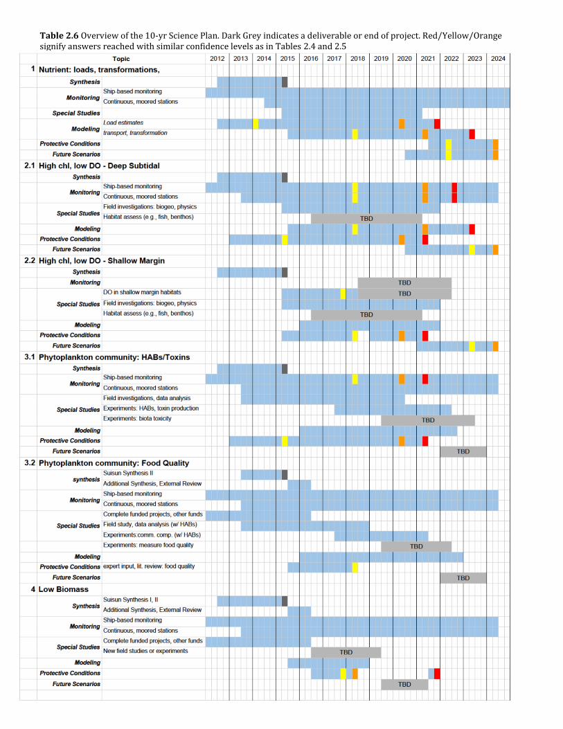
2.6 10-year Science Plan This section presents the 10-year Science Plan at a few different resolutions. Figure 2.6 depicts the approximate timing of major activities within the main Work Categories across all Program Areas. Table 2.6 provides more detail, breaking down work into Program Areas, Work Categories, and major activities. A more granular version of Table 2.6 is presented in Table A.2, which illustrates the full breadth of science needs. Despite what may look like a very detailed portrayal of activities in Table A.2, the project descriptions are still quite general, and specific data needs will need to be identified on a year-by-year basis, and prioritized as the program progresses. The Science Plan project timelines (Tables 2.6 and A.2) and milestone timing (Table 2.4-2.5) present realistic estimates of the time required to conduct investigations and reach reasonably confident answers to management questions. As noted in Section 2.4, the plan is not constrained by the current budget, which is ~$1.4mill yr-1. Pursuing all of these topics in parallel would require a much higher funding level.

14
Figure 2.6 Approximate timing of major work categories over a 10 year Science Plan.
Although Figure 2.6 and Table 2.6 present the timing of work, and forecasted times for answering management questions, they do not convey the workflow or iterative nature of activities. Sidebar A provides three examples to better illustrate the Science Plan’s workflow and iterative structure. The workflows in Sidebar A are analogous in structure to the tiered workflow example in Section 2.5, with those in Sidebar A providing some additional detail (specific to pathways) and illustrating the recommended iterative nature of the workflow.
15
Table 2.6 Overview of the 10-yr Science Plan. Dark Grey indicates a deliverable or end of project. Red/Yellow/Orange signify answers reached with similar confidence levels as in Tables 2.4 and 2.5

16
Table 2.6 cont’d
2.7 Projects identified for FY2016-2018 Table 2.7 summarizes projects that were identified within the 10-year plan (Figure A.2) as beginning in FY2016-2018. Table 2.7 also notes the geographic focus of each investigations and the target Program Areas, as well as estimated costs. A next important step is to prioritize among these projects to identify those projects that should go forward in FY2016, recognizing that their estimated total cost exceeds current funding.

1
7
Ta
ble
2.7

18

Iden
%fy(Protec%ve(Co
ndi%on
s((Assessm
ent(F
ramew
ork)(
Redirect(effo
rts(
toward(othe
r(pathways(
Con3
nue(
Mon
itorin
g.(
Figure S.1
Figure S.2
Side
bar A
Each m
ajor Program
Area could be
thou
ght o
f as h
aving its own
sub-‐plan (Figure S.1 and S.2). Som
e projects or a
cBviBe
s may be
disBnct to on
e program area, and
others m
ay con
tribute to
mulBp
le program
areas (verBcally).
Figure S.3 is a gen
eral example, while Figure S.4 and Figure S.5
presen
t the
cases fo
r HAB
s/toxins and
Low
DO in slou
ghs/creeks,
respecBvely. Enter th
e diagram in th
e pu
rple “Iden
Bfy ProtecBve
Cond
iBon
s” box, and
proceed
to th
e “Adverse Im
pact?” decision
. For m
ost o
f the
Program
Areas, the
re re
mains con
siderable
uncertainty abou
t whe
ther adverse im
pacts a
re occurrin
g and
the do
se:re
spon
se with
nutrie
nts, which leads into the
Mon
itorin
g and Special Studies box. The
smaller rectangles
illustrate the type
s of studies or a
cBviBe
s that w
ould be pu
rsue
d du
ring a pass th
rough the Mon
itorin
g and Special Studies box.
One
pass throu
gh th
is bo
x, carrying ou
t mulBp
le acBviBe
s in
parallel (e.g., m
onito
ring, field invesBgaBo
ns) to gene
rate new
data or test h
ypothe
ses, wou
ld ta
ke ~3 years. That n
ew
inform
aBon
wou
ld be used
to provide
provisio
nal answers to
managem
ent q
uesBon
s (Tables 2.4-‐2.5) and
refin
e the
Assessmen
t Framew
ork (AF).
The process rep
eats unB
l the
ambien
t con
diBo
n data and
AF
have develop
ed to
the po
int w
here “Ad
verse Im
pact?“ can be
answ
ered
with
sufficien
t con
fiden
ce. Exactly what con
sBtutes
sufficien
t con
fiden
ce is a re
gulatory decision
or m
anagem
ent
decisio
n. If the
re is an adverse im
pact, w
ork moves to
revisin
g concep
tual m
odels, develop
ing and im
plem
enBn
g nu
merical
mod
els, invesBgaBn
g the qu
anBtaB
ve im
portance of n
utrie
nts,
and exploring load re
ducBon
scen
arios that w
ould m
iBgate
impairm
ent. As n
oted
abo
ve, w
ork wou
ld likely proceed
on
mulBp
le fron
ts in parallel, no
t in serie
s – fo
r example, work will
have been moving forw
ard with
mod
el develop
men
t, and whe
n mod
eling is ne
eded
to answer a sp
ecific qu
esBo
n, th
e Ba
se
Mod
el will re
ady for u
se and
customiza
Bon for the
specific
quesBo
ns being explored.
19

Iden
tify
prot
ectiv
e co
nditi
ons
for
bene
ficia
l use
- exi
stin
g da
ta
- exp
ert i
nput
- f
ield
sur
veys
- e
xper
imen
ts
Redirect effo
rts
toward othe
r pathways.
ConB
nue
Mon
itorin
g.
Figure S.3 Gen
eral Case
20

Figure S.4 H
ABs/toxins
Redirect(effo
rts(
toward(othe
r(pathways(
Con3
nue(
Mon
itorin
g.(
21

Figure S.5 Low DO: sloughs, creeks
Redirect effo
rts
toward othe
r pathways.
ConB
nue Mon
itorin
g.
Mec
hani
stic
fiel
d st
udie
s an
d da
ta
colle
ctio
n
22

23
Appendix 1 Additional Science Plan Tables

24
Tie
r Q
ues
tio
n
Cu
rren
t le
vel
of
com
ple
tio
n
Co
nfi
den
ce
if a
nsw
er
giv
en t
od
ay
Co
st a
nd
act
ivit
y
Tim
e to
co
mp
lete
To
tal
Co
st
($1
00
0s)
Fea
sib
le t
o
answ
er b
y
20
24
?
1
Are
HA
Bs/
NA
Bs/
toxi
ns
pre
sen
t? I
f so
w
hic
h o
nes
, ho
w a
bu
nd
ant?
20
%
Exi
stin
g d
ata
sho
w p
rese
nce
co
mm
on
det
ecti
on
of
HA
B
spec
ies
To
xin
s ar
e u
biq
uit
ou
s b
ut
effe
ct is
un
kn
ow
n
Hig
h
$1
50
/yr
1 m
ore
yea
r o
f sa
mp
le
coll
ecti
on
1.5
yr
$2
25
Y
es
2
Are
HA
Bs
cau
sin
g im
pai
rmen
t, b
ased
on
ex
isti
ng
dat
a o
n w
hat
cau
ses
adv
erse
im
pac
ts e
lsew
her
e, a
nd
bas
ed o
n t
oxi
n
con
cen
trat
ion
s in
bio
ta a
nd
wat
er?
10
%
To
xin
s ar
e u
biq
uit
ou
s in
w
ater
. T
oxi
ns
hav
e al
so b
een
d
etec
ted
in
mo
st b
ival
ve
sam
ple
s an
aly
zed
to
dat
e, b
ut
are
gen
eral
ly lo
w r
elat
ive
to
exis
tin
g g
uid
ance
lev
els.
Lo
w
$2
00
/yr
Biv
alv
e sa
mp
lin
g, w
ater
co
lum
n s
amp
lin
g.
Ad
dit
ion
al 2
-3 y
ears
of
dat
a.
4 y
r $
80
0
Yes
3
Wh
at a
re t
he
eco
logi
cal d
riv
ers
at a
la
rge
scal
e, i
n p
arti
cula
r th
e ro
le o
f n
utr
ien
ts (
alo
ngs
ide
oth
er
ph
ysi
cal/
bio
logi
cal f
acto
rs)?
10
%
Som
e d
ata
avai
lab
le, m
ore
n
eed
ed. 3
-5 a
dd
itio
nal
yea
rs
of
dat
a.
Lo
w
$1
50
/yr
Ad
dit
ion
al s
amp
le
anal
ysi
s, d
ata
anal
ysi
s an
d
inte
rpre
tati
on
3 y
r $
45
0
Yes
4
Wh
at a
re t
he
ph
ysi
olo
gica
l dri
ver
s? I
n
par
ticu
lar
wh
at r
ole
s d
o n
utr
ien
ts p
lay
, an
d w
hat
wo
uld
be
pro
tect
ive
con
cen
trat
ion
s?
5%
B
ased
on
stu
die
s in
oth
er
syst
ems
Lo
w
$1
50
-20
0/y
r Su
bst
anti
al u
nd
erta
kin
g
6+
yea
rs
e.g.
, 3 y
r fo
r ea
ch c
lass
of
org
anis
ms
>$
10
00
Y
es
5
Is a
cute
or
chro
nic
im
pai
rmen
t fr
om
to
xin
s ev
iden
t in
res
iden
t o
rgan
ism
s?
0%
N
o d
ata
Lo
w
$1
00
-20
0/y
r L
ab e
xper
imen
ts o
r ti
ssu
e fr
om
Bay
an
imal
s 5
+ y
rs
>$
10
00
Y
es
6
Pre
dic
tiv
e/st
atis
tica
l mo
del
s: I
s th
ere
a n
utr
ien
t-re
late
d h
igh
ris
k?
Wh
at le
vel
s o
f n
utr
ien
ts w
ou
ld b
e p
rote
ctiv
e?
0%
N
eed
eco
logi
cal a
nd
p
hy
sio
logi
cal r
esu
lts
fro
m 3
an
d 4
, an
d d
ata
fro
m 1
an
d 2
.
Lo
w
$1
50
/yr
3 y
rs
$4
50
Yes
, bu
t #
2-4
wo
uld
n
eed
to
st
art
earl
y
7
Nu
mer
ical
sim
ula
tio
n m
od
els:
Is
ther
e a
nu
trie
nt-
rela
ted
hig
h r
isk
? W
hat
lev
els
of
nu
trie
nts
wo
uld
be
pro
tect
ive?
0%
N
eed
mu
ch d
ata
on
gro
wth
co
nd
itio
ns
Lo
w
$2
00
Se
mi-
qu
anti
tati
vel
y
imp
rov
ed u
nd
erst
and
ing
of
nu
trie
nt
role
an
d r
isk
5 y
ears
of
mo
del
d
evel
op
men
t $
10
00
N
ot
to
com
ple
tio
n
Ta
ble
A.1
Tie
red
ord
erin
g o
f H
AB
s/to
xin
s q
ues
tio
ns
and
est
imat
ed e
ffo
rt a
sso
ciat
ed w
ith
wo
rk. N
ote
: In
gen
eral
th
e co
sts
incl
ud
ed h
ere
do
n
ot
incl
ud
e th
e co
sts
asso
ciat
ed w
ith
ro
uti
ne
mo
nit
ori
ng
(fi
eld
wo
rk)
to c
oll
ect
sam
ple
s, o
r co
st o
f an
cill
ary
dat
a (n
utr
ien
ts, T
, sal
, lig
ht,
etc
.).

25
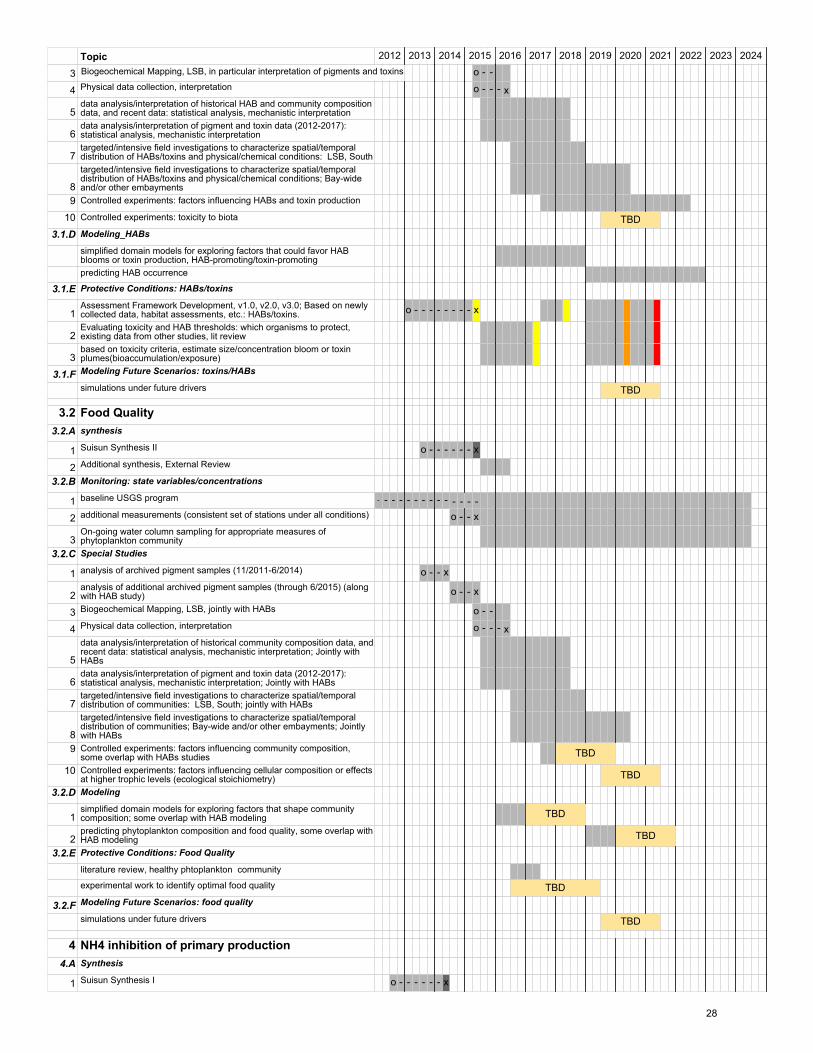
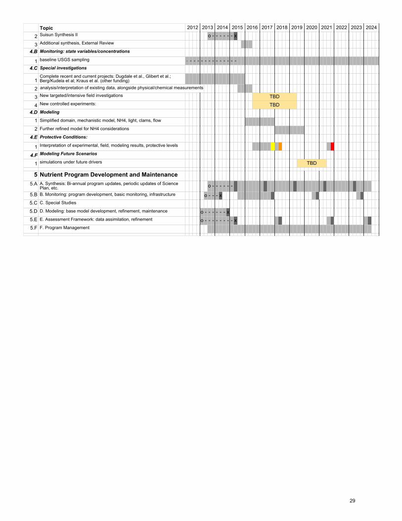
Table A.2 10-year Science Plan o - - - - - - - x Indicates a project that was/is funded and is completed or still underway Dark grey squares indicate a deliverable or report (there are more deliverables than noted in table; just a subset here) The yellow, orange and red cells indicate a milestone for answers being iteratively reached to questions that are closely tied to management questions (initial, medium, and final, respectively), corresponding to Tables 2.4 and 2.5.

TopicFirst 5 year Watershed Permit cycle.
Second 5-year permit.
1. Nutrient: loads, fate, transport1.A Synthesis_Nutrients
1 conceptual model o - - - - - - - x
2 LSB synthesis o - - - - - - x
3 Suisun Synthesis I o - - - - - - x1.B Monitoring_Nutrients
1 Baseline Nutrient monitoring: monthly, bi-weekly, Bay-wide - - - - - - - - - - - - - -
2 Additional new parameters, shifting toward new nutrient program o - - x
3 Continuous, moored stations, LSB and South Bay focus, nutrients o - - x
4 Continuous, moored stations, other subembayments, nutrients
1.C Special investigations: rates, physics, state variables_Nutrients
1 Biogeochemical Mapping, LSB focus o - - x
2 Physical data collection, interpretation, LSB and South Bay focus o - - - x
3N and P transformations and uptake, field investigations, physical data,LSB and South Bay focus
4N/P transformations, field investigations, physical data, othersubembayments
1.D Modeling
Load estimates
1 Overall Loading estimates, v1.0, v2.0, ... o - - - - - x
2 Delta loads to Suisun, v1.0, v2.0 o - - - - - x
3 Refined point source load estimates, v1.0, v2.0, ...
4 Local watershed load estimates
transport, transformation
5 Subsystem: LSB and South Bay, including sensitivity analysis o - - x
6 Subsystem: Suisun Bay, including sensitivity analysis
7 Bay-wide nutrient transformations + transport; source tracking/attribution
8 Exchange with coastal ocean, fate of exported nutrients
1.E Protective Conditions: nutrients
1 Based on protective levels for DO, HABs, etc, determine protectivenutrient concentrations or loads
1.F Future Scenarios: Nutrients
1 Nutrient cycling/concentrations under future land uses
2 Future scenarios for nutrient inputs (e.g., load reductions)
2 High chl, low DO2.1 2.1 DO: deep subtidal
2.1.A Synthesis
1 conceptual model o - - - - - - - x
2 LSB synthesis o - - - - - - x2.1.B Monitoring: state variables/concentrations
1 Baseline biomass monitoring: monthly, bi-weekly, Bay-wide - - - - - - - - - - - - - -
2 Additional new parameters, shifting toward new nutrient program o - - x
3 Continuous, moored stations, LSB and South Bay focus, biomass/DO - - - - - - - x4 Continuous, moored stations, other subembayments, bioimass/DO
2.1.C Special investigations: rates, physics, state variables, chl-DO deep
1 Biogeochemical Mapping, LSB o - - x
2 Physical data collection, interpretation, LSB o - - - x
3
LSB and South Bay focused field investigations: Biomass, productivity,respiration/oxygen demand in water column and sediments, grazing,physical observations (stratification, velocities, etc.)
4
field investigations, other embayments: Biomass, productivity,respiration/oxygen demand in water column and sediments, grazing,physical observations (stratification, velocities, etc.)
5 Habitat/condition assessments (e.g., fish surveys, benthos)
6 Controlled studies on DO/T tolerance for target species
2.1.D Modeling_chl-DO_deep
2012 2013 2014 2015 2016 2017 2018 2019 2020 2021 2022 2023 2024
TBD
26

Topic
1
Subsystem: LSB and South Bay, focus on explaining recent changes,including sensitivity analysis, relative imporantance of regulating factors(clams, light, etc.)
o - - x
2
Subsystem: Suisun, focus on explaining past changes, relativeimportance of factors (light, NH4, clams, flushing), including sensitivityanalysis
3 Bay-wide biomass/production/DO
4Exchange with coastal ocean, fate of exported biomass, importance ofimported biomass
2.1.E Protective Conditions: DO,chl_deep
1
Assessment Framework Development, v1.0, v2.0, v3.0; Based on newlycollected data, model simulations, habitat assessments, and anyrefinements to DO standards
o - - - - - - - - x
2 Evaluating DO standards: literature review, desktop studies o - - x
2.1.F Modeling Future Scenarios: DO, deep subtidal
1 DO, productivity, biomass, etc., under environmental change scenarios
2 Future scenarios for management actions (e.g., load reductions)
2.2 DO: shallow margin2.2.A Synthesis
1 conceptual model o - - - - - - - x
2 o - - - - - - x
3 Suisun Marsh TMDL work (separate effort)
2.2.B Monitoring: state variables/concentrations
1 On-going monitoring in sloughs, or special studies?
2.2.C Special investigations: rate measurements, physics, state variables
1 DO in shallow margin habitats, LSB focus o - - - x
2 Biogeochemical Mapping, LSB o - - x
3 Physical data collection, interpretation, LSB o - - - x
4
LSB and South Bay focused field investigations: Biomass, productivity,respiration/oxygen demand in water column and sediments, grazing,physical observations (stratification, velocities, etc.)
5
field investigations, other embayments: Biomass, productivity,respiration/oxygen demand in water column and sediments, grazing,physical observations (stratification, velocities, etc.)
6 Habitat/condition assessments (e.g., fish surveys, benthos)
7 Controlled studies on DO/T tolerance for target species
2.2.D Modeling_chl-DO_shallow
1Slough modeling: focus on one representative sloughs in LSB or SouthBay, biomass/DO, nutrients; starting basic, adding complexity as needed
2 Expand to other sloughs/creeks, as needed and feasible
2.2.E Protective Conditions: DO_shallow
1
Assessment Framework Development, v1.0, v2.0, v3.0; Based on newlycollected data, model simulations, habitat assessments, and anyrefinements to DO standards
2 Evaluating DO standards: literature, desktop studies o - - x
2.2.F Modeling Future Scenarios: DO, deep shallow
1 DO, productivity, biomass, etc., under environmental change scenarios
2 Future scenarios for management actions (e.g., load reductions)
3 Phytoplankton community3.1 HABs/toxins
3.1.A Synthesis: HABs/toxins
1 conceptual model o - - - - - - - x
2 Suisun Synthesis 2 o - - - - - - x3.1.B Monitoring: state variables/concentrations
1 baseline USGS program - - - - - - - - - - - - - -
2 integrative measurements (SPATT on Polaris, or at fixed sites) - - - - - - - - - - - x
3 additional measurements (consistent set of stations under all conditions) o - - x
4 On-going water column sampling for toxins
5 Benthos monitoring (natural organisms or e.g., mussel watch)
3.1.C Special investigations
1analysis of archived pigment samples; on-going analysis of samplescollected during monitoring o - - x
2analysis of archived toxin samples (11/2011-12/2014); on-going analysisof samples collected during monitoring o - - x
2012 2013 2014 2015 2016 2017 2018 2019 2020 2021 2022 2023 2024
LSB synthesis (including Analysis of existing DO data in Lower South Bay)
TBD
TBD
TBD
27
Topic3 o - -
4 Physical data collection, interpretation o - - - x
5data analysis/interpretation of historical HAB and community compositiondata, and recent data: statistical analysis, mechanistic interpretation
6data analysis/interpretation of pigment and toxin data (2012-2017):statistical analysis, mechanistic interpretation
7targeted/intensive field investigations to characterize spatial/temporaldistribution of HABs/toxins and physical/chemical conditions: LSB, South
8
targeted/intensive field investigations to characterize spatial/temporaldistribution of HABs/toxins and physical/chemical conditions; Bay-wideand/or other embayments
9 Controlled experiments: factors influencing HABs and toxin production
10 Controlled experiments: toxicity to biota
3.1.D Modeling_HABs
simplified domain models for exploring factors that could favor HABblooms or toxin production, HAB-promoting/toxin-promotingpredicting HAB occurrence
3.1.E Protective Conditions: HABs/toxins
1Assessment Framework Development, v1.0, v2.0, v3.0; Based on newlycollected data, habitat assessments, etc.: HABs/toxins. o - - - - - - - - x
2Evaluating toxicity and HAB thresholds: which organisms to protect,existing data from other studies, lit review
3based on toxicity criteria, estimate size/concentration bloom or toxinplumes(bioaccumulation/exposure)
3.1.F Modeling Future Scenarios: toxins/HABs
simulations under future drivers
3.2 Food Quality3.2.A synthesis
1 Suisun Synthesis II o - - - - - - x
2 Additional synthesis, External Review
3.2.B Monitoring: state variables/concentrations
1 baseline USGS program - - - - - - - - - - - - - -
2 additional measurements (consistent set of stations under all conditions) o - - x
3On-going water column sampling for appropriate measures ofphytoplankton community
3.2.C Special Studies
1 analysis of archived pigment samples (11/2011-6/2014) o - - x
2analysis of additional archived pigment samples (through 6/2015) (alongwith HAB study) o - - x
3 Biogeochemical Mapping, LSB, jointly with HABs o - -
4 Physical data collection, interpretation o - - - x
5
data analysis/interpretation of historical community composition data, andrecent data: statistical analysis, mechanistic interpretation; Jointly withHABs
6data analysis/interpretation of pigment and toxin data (2012-2017):statistical analysis, mechanistic interpretation; Jointly with HABs
7targeted/intensive field investigations to characterize spatial/temporaldistribution of communities: LSB, South; jointly with HABs
8
targeted/intensive field investigations to characterize spatial/temporaldistribution of communities; Bay-wide and/or other embayments; Jointlywith HABs
9 Controlled experiments: factors influencing community composition,some overlap with HABs studies
10 Controlled experiments: factors influencing cellular composition or effectsat higher trophic levels (ecological stoichiometry)
3.2.D Modeling
1simplified domain models for exploring factors that shape communitycomposition; some overlap with HAB modeling
2predicting phytoplankton composition and food quality, some overlap withHAB modeling
3.2.E Protective Conditions: Food Quality
literature review, healthy phtoplankton community
experimental work to identify optimal food quality
3.2.F Modeling Future Scenarios: food quality
simulations under future drivers
4 NH4 inhibition of primary production4.A Synthesis
1 Suisun Synthesis I o - - - - - - x
2012 2013 2014 2015 2016 2017 2018 2019 2020 2021 2022 2023 2024Biogeochemical Mapping, LSB, in particular interpretation of pigments and toxins
TBD
TBD
TBD
TBD
TBD
TBD
TBD
TBD
28
Topic2 Suisun Synthesis II o - - - - - - x
3 Additional synthesis, External Review
4.B Monitoring: state variables/concentrations
1 baseline USGS sampling - - - - - - - - - - - - - -4.C Special investigations
1Complete recent and current projects: Dugdale et al., Glibert et al.;Berg/Kudela et al; Kraus et al. (other funding)
2
3 New targeted/intensive field investigations
4 New controlled experiments:
4.D Modeling
1 Simplified domain, mechanistic model, NH4, light, clams, flow
2 Further refined model for NH4 considerations
4.E Protective Conditions:
1 Interpretation of experimental, field, modeling results, protective levels
4.F Modeling Future Scenarios
1 simulations under future drivers
5 Nutrient Program Development and Maintenance5.A A. Synthesis: Bi-annual program updates, periodic updates of Science
Plan, etc. o - - - - - -
5.B B. Monitoring: program development, basic monitoring, infrastructure o - - - x5.C C. Special Studies
5.D D. Modeling: base model development, refinement, maintenance o - - - - - - x5.E E. Assessment Framework: data assimilation, refinement o - - - - - - - - x5.F F. Program Management
2012 2013 2014 2015 2016 2017 2018 2019 2020 2021 2022 2023 2024
analysis/interpretation of existing data, alongside physical/chemical measurements
TBD
TBD
TBD
29

30
Appendix 2. BackgroundA.2.1 San Francisco Bay and the Bay AreaSan Francisco Bay (SFB) encompasses several subembayments of the San Francisco Estuary, thelargest estuary in California (Figure A.2.1). SFB is surrounded by remnant tidal marshes, intertidaland subtidal habitats, tributary rivers, the freshwater “Delta” portion of the estuary, and the largemixed-land-use area known as the San Francisco Bay Area (Figure A.2.2.A). San Francisco Bayhosts an array of habitat types (Figure A.2.1), many of which have undergone substantial changes intheir size or quality due to human activities. Urban residential and commercial land uses comprise alarge portion of Bay Area watersheds, in particular those adjacent to Central Bay, South Bay andLower South Bay (Figure A.2.2.A). Open space and agricultural land uses occupy larger proportions
of the watersheds draining to Suisun Bay and San Pablo Bay. The San Joaquin and Sacramento Rivers drain 40% of California, including agricultural-intensive land use areas in the Central Valley. Flows from several urban centers also enter these rivers, most notably Sacramento which is ~100 km upstream of Suisun Bay along the Sacramento River.
SFB receives high nutrient loads from 42 public owned wastewater treatment works (POTWs) servicing the Bay Area’s 7.2 million people (Figure A.2.2.B). Several POTWs carry out nutrient removal before effluent discharge; however the majority perform only secondary treatment without additional N or P removal. Nutrients also enter SFB via stormwater runoff from the densely populated watersheds that surround SFB (Figure A.2.2.A). Flows from the Sacramento and San Joaquin Rivers deliver large nutrient loads, and enter the northern estuary through the Sacramento/San Joaquin Delta (not shown, immediately east of the maps in Figure A.2.1 and A.2.2).Figure A.2.1 Habitat types of SFB and surrounding Baylands.
Water Board subembayments boundaries are shown in black. Habitat data from CA State Lands Commission, USGS, UFWS, US NASA and local experts were compiled by SFEI.
31
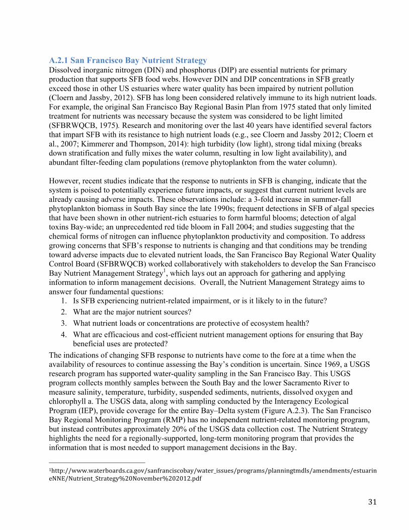
A.2.1 San Francisco Bay Nutrient StrategyDissolved inorganic nitrogen (DIN) and phosphorus (DIP) are essential nutrients for primaryproduction that supports SFB food webs. However DIN and DIP concentrations in SFB greatlyexceed those in other US estuaries where water quality has been impaired by nutrient pollution(Cloern and Jassby, 2012). SFB has long been considered relatively immune to its high nutrient loads.For example, the original San Francisco Bay Regional Basin Plan from 1975 stated that only limitedtreatment for nutrients was necessary because the system was considered to be light limited(SFBRWQCB, 1975). Research and monitoring over the last 40 years have identified several factorsthat impart SFB with its resistance to high nutrient loads (e.g., see Cloern and Jassby 2012; Cloern etal., 2007; Kimmerer and Thompson, 2014): high turbidity (low light), strong tidal mixing (breaksdown stratification and fully mixes the water column, resulting in low light availability), andabundant filter-feeding clam populations (remove phytoplankton from the water column).
However, recent studies indicate that the response to nutrients in SFB is changing, indicate that the system is poised to potentially experience future impacts, or suggest that current nutrient levels are already causing adverse impacts. These observations include: a 3-fold increase in summer-fall phytoplankton biomass in South Bay since the late 1990s; frequent detections in SFB of algal species that have been shown in other nutrient-rich estuaries to form harmful blooms; detection of algal toxins Bay-wide; an unprecedented red tide bloom in Fall 2004; and studies suggesting that the chemical forms of nitrogen can influence phytoplankton productivity and composition. To address growing concerns that SFB’s response to nutrients is changing and that conditions may be trending toward adverse impacts due to elevated nutrient loads, the San Francisco Bay Regional Water Quality Control Board (SFBRWQCB) worked collaboratively with stakeholders to develop the San Francisco Bay Nutrient Management Strategy1, which lays out an approach for gathering and applying information to inform management decisions. Overall, the Nutrient Management Strategy aims to answer four fundamental questions:
1. Is SFB experiencing nutrient-related impairment, or is it likely to in the future?2. What are the major nutrient sources?3. What nutrient loads or concentrations are protective of ecosystem health?4. What are efficacious and cost-efficient nutrient management options for ensuring that Bay
beneficial uses are protected?The indications of changing SFB response to nutrients have come to the fore at a time when the availability of resources to continue assessing the Bay’s condition is uncertain. Since 1969, a USGS research program has supported water-quality sampling in the San Francisco Bay. This USGS program collects monthly samples between the South Bay and the lower Sacramento River to measure salinity, temperature, turbidity, suspended sediments, nutrients, dissolved oxygen and chlorophyll a. The USGS data, along with sampling conducted by the Interagency Ecological Program (IEP), provide coverage for the entire Bay–Delta system (Figure A.2.3). The San Francisco Bay Regional Monitoring Program (RMP) has no independent nutrient-related monitoring program, but instead contributes approximately 20% of the USGS data collection cost. The Nutrient Strategy highlights the need for a regionally-supported, long-term monitoring program that provides the information that is most needed to support management decisions in the Bay.
1http://www.waterboards.ca.gov/sanfranciscobay/water_issues/programs/planningtmdls/amendments/estuarineNNE/Nutrient_Strategy%20November%202012.pdf

32
The timing also coincides with a major state-wide initiative, led by the California State Water Resources Control Board (State Water Board), for developing nutrient water quality objectives for the State’s surface waters, using an approach known as the Nutrient Numeric Endpoint (NNE) framework. The NNE framework establishes a suite of numeric endpoints based on the ecological response of a waterbody to nutrient over-enrichment and eutrophication (e.g. excessive algal blooms, decreased dissolved oxygen). In addition to numeric endpoints for response indicators, the NNE approach includes models that link the response indicators to nutrient loads and other management controls. The NNE framework is intended to serve as numeric guidance to translate narrative water quality objectives.

33
Figu
re A
.2.2
A. L
and
use
in w
ater
shed
s tha
t dra
in to
SFB
(Dat
a fr
om A
ssoc
iatio
n of
Bay
Are
a G
over
nmen
ts, 2
000)
. B. L
ocat
ion
and
desi
gn
size
(in
mill
ion
gallo
ns p
er d
ay) f
or P
OTW
s th
at d
isch
arge
dire
ctly
in S
FB o
r in
wat
ersh
eds d
irect
ly a
djac
ent t
o su
bem
baym
ents
. In
both
fig
ures
, Wat
er B
oard
sube
mba
ymen
t bou
ndar
ies
are
show
n in
bla
ck.

34
Since San Francisco Bay is California’s largest estuary, it is a primary focus of the state-wide effort to develop NNEs for estuaries. Through the Nutrient Strategy, the SFBRWQCB is working with regional stakeholders and with the State Water Board to develop an NNE framework specific to SFB. That effort was initiated by a literature review and data gaps analysis that recommends indicators to assess eutrophication and other adverse effects of nutrient overenrichment in San Francisco Bay McKee et al., 2011)2. McKee et al. (2011) evaluated a number of potential indicators of ecological condition for several habitat types based on the following criteria: • Indicators should have well-documented links to estuarine beneficial uses• Indicators should have a predictive relationship with nutrient and hydrodynamic drivers that can
be easily observed with empirical data or a model• Indicators should have a scientifically sound and practical measurement process that is reliable
in a variety of habitats and at a variety of timescales• Indicators must be able to show a trend towards increasing or/and decreasing benefical use
impairment due to nutrientsThe report recommended focusing on subtidal habitats initially, and proposed the following primary indicators of beneficial use impairment by nutrients: i. phytoplankton biomass; ii. phytoplankton composition; iii. dissolved oxygen; and; iv. algal toxin concentrations. In addition, ‘supporting indicators’ and ‘co-factors’ were identified, and are summarized in Table A.2.1. Supporting indicators provide additional lines of evidence to complement observations based on primary indicators, and co-factors are essential information to help interpret and analyze trends in primary or supporting indicators.
Table A.2.1 Recommended indicators within the context of the SFB NNE. Excerpted from McKee et al 2011
Habitat Primary Indicators Supporting Indicators Co-Factors All Subtidal Habitat
Phytoplankton biomass, productivity and assemblage Cyanobacteria cell counts and toxin concentration Dissolved oxygen
Water column nutrient concentrations and forms1 (C,N,P,Si) HAB species cell counts and toxin concentration
Water column turbidity, pH, conductivity, temperature, light attenuation Macrobenthos taxonomic composition, abundance and biomass Sediment oxygen demand Zooplankton
Seagrass Habitat
Phytoplankton biomass Macroalgal biomass & cover Dissolved oxygen
Light attenuation, suspended sediment concentration Seagrass areal distribution and cover Epiphyte load
Water column pH, temperature, conductivity Water column nutrients
Intertidal flats Macroalgal biomass and cover Sediment % OC, N, P and particle size Microphytobenthos biomass (benthic chl-a)
Microphytobenthos taxonomic composition
Muted Intertidal and Subtidal
Macroalgal biomass & cover Phytoplankton biomass Cyanobacteria toxin concentration
Sediment % OC, N, P and particle size Phytoplankton assemblage Harmful algal bloom toxin concentration
Water column pH, turbidity, temperature, conductivity Water column nutrients
2http://www.waterboards.ca.gov/sanfranciscobay/water_issues/programs/planningtmdls/amendments/estuarineNNE/644_SFBayNNE_LitReview%20Final.pdf

35
Figure A.2.3 Location of DWR/IEP and USGS monthly sampling stations. Data from labeled USGS Stations (s6, s15, s18, s21, s27, s36) are used in Figures 5.7, 6.3-6.7 and 7.11.
Regions of SFB behave quite differently with respect to nutrient cycling and ecosystem response due to a combination physical, chemical, and biological factors. To facilitate the discussion of spatial trends in this report, SFB was divided into 5 subembayments, as depicted in Figure A.2.1: Suisun Bay, San Pablo Bay, Central Bay, South Bay and Lower South Bay (LSB). These subembayment boundaries were chosen based on geographic features and not necessarily hydrodynamic features, represent one of several sets of boundaries that could be used. The boundaries illustrated in Figure A.2.1 are similar to those defined by the SFBRWQCB in the San Francisco Bay Basin Plan, although we use different names for the subembayments south of the Bay Bridge.

36
Appendix 3 Problem Statement A.3.1 Recent observations in SFBIn estuarine ecosystems in the US and worldwide, high nutrient loads and elevated nutrientconcentrations are associated with multiple adverse impacts (Bricker et al. 2007). N and P areessential nutrients for the primary production that supports food webs in SFB and other estuaries.However, when nutrient loads reach excessive levels they can adversely impact ecosystemhealth. Individual estuaries vary in their response or sensitivity to nutrient loads, with physicaland biological characteristics modulating estuarine response (e.g., Cloern 2001). As a result,some estuaries experience limited or no impairment at loads that have been shown to havesubstantial impacts elsewhere.
Figure A.3.1 illustrates several potential pathways along which excessive nutrient loads could adversely impact ecosystem health in SFB. Each pathway is comprised of multiple linked physical, chemical, and biological processes. Some of those processes are well-understood and data are abundant data to interpret and assess condition; others are poorly understood or data are scarce. A recent conceptual model report (SFEI 2014a) describes the processes creating the pathways between loads and adverse response, and describes the current state of knowledge and data availability.
Figure A.3.1 Potential adverse impact pathways: linkages between anthropogenic nutrient loads and adverse impacts on uses or attributes of SFB. The shaded rectangles represent indicators that could actual be measured along each pathway to assess condition. Grey rectangles to the right represent uses or attributes of SFB for which water quality is commonly managed. Yellow circles indicate the forms of nutrients that are relevant for each pathway

37
Current nutrient loads to some SFB subembayments are comparable to or much greater than those in a number of other major estuaries that experience impairment from nutrient overenrichment (SFEI 2014). Consistent with its high loads, SFB has elevated levels of dissolved inorganic nitrogen (DIN) and dissolved inorganic phosphorous (DIP) relative to other estuaries (Figure A.3.2). Yet SFB does not commonly experience classic symptoms of nutrient overenrichment, such as massive and sustained phytoplankton blooms, or low dissolved oxygen over large areas in the subtidal zone. SFB has been spared the most obvious adverse impacts of high nutrient loads along these pathways due to a combination of factors (high turbidity; strong tidal mixing; large populations of benthic filter feeders) that have imparted SFB with some inherent resistance to these effects (Cloern and Jassby, 2012; SFEI 2014). However, several recent sets of observations indicate that nutrient-related problems may already be occurring in some areas of SFB, or serve as early warnings of problems on the horizon.
Figure A.3.2 Nutrient concentrations in South Bay compared to other estuaries. Source: Cloern and Jassby (2012)
Over the past 15 years, statistically significant increases in phytoplankton biomass have been observed throughout SFB. Most notably summer/fall phytoplankton biomass tripled between the mid-1990s and the mid-2000s (Figure A.3.3; Cloern et al., 2007) in South Bay and LSB, representing a shift in trophic status from oligo-mesotrophic (low to moderate productivity system) to meso-eutrophic (moderate to high productivity system) (Cloern and Jassby, 2012).
Figure A.3.3 Interquartile range of Aug-Dec chl-a concentrations averaged across all USGS stations between Dumbarton Bridge and Bay Bridge, 1977-2005. Source: Cloern et al., 2007

38
More recent data from South Bay suggest that, at least presently, biomass concentrations have plateaued at a new level instead of continuing to rise (Figure A.3.4). While the greatest magnitudes of biomass increase (i.e., in ug/L chl-a) have been observed in South Bay, other SFB subembayments have also experienced statistically significant increases in phytoplankton biomass (J Cloern, personal communication).
Figure A.3.4 Same stations as and data as presented Figure A.3.5, with data extendedthrough 2013 (Interquartilerange of Aug-Dec chl-aconcentrations averaged acrossall USGS stations betweenDumbarton Bridge and BayBridge, 1977-2013). Source:SFEI 2014c
In Suisun Bay, extremely low phytoplankton biomass has defined the system since 1987 (Figure A.3.8), coincident in time with the invasive clam, Potamocorubula amurensis, becoming widelyestablished. The extended period of low phytoplankton biomass and low rates of primaryproduction are considered to be among the factors contributing to long-term declines in uppertrophic level production in Suisun Bay and the Delta by limiting food supply (Baxter et al., 2010;NRC 2012). While the low phytoplankton biomass and productivity in Suisun Bay have
frequently been attributed to the impacts of Potamocorbula and low light levels due to high suspended sediments (e.g., Kimmerer and Thompson, 2014), recent studies have argued that elevated ammonium (NH4
+) concentrations in Suisun Bay also limit primary production rates and play an important role in both creating the low biomass conditions and exacerbating food limitation (Dugdale et al., 2007; Dugdale et al., 2012; Parker et al. 2012a,b). Other studies have proposed that high ambient concentrations of nitrate (NO3
-) and NH4+, and
altered ratios of N:P cause shifts phytoplankton community composition toward
Figure A.3.5 Phytoplankton biomass in Suisun Bay, 1975-2010. Source: J Cloern, USGS; Data: USGS, DWR-EMP

39
species having poor food quality, adversely impacting Delta food webs (Glibert 2010; Glibert et al., 2011).
Harmful phytoplankton species also represent a growing concern. The harmful algae, Microcystis spp., and the toxin they produce, microcystin, have been detected with increasing frequency in the Delta and Suisun Bay since ~2000 (Lehman et al., 2008). In addition, the HAB toxins microcystin and domoic acid have been detected Bay-wide (Figure A.3.6). The ecological
Figure A.3.6 HAB toxins detected in SFB during 2011. Bars represent 1 SD for salinity and temperature Source: R. Kudela
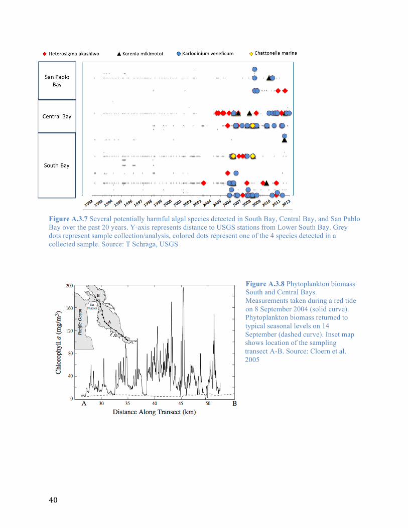
significance of observed toxin levels in the Bay are not yet known. A number of phytoplankton species that have formed harmful algal blooms (HABs) in other systems have been detected throughout SFB (Figure A.3.7 and Table A.3.1). Although the abundances of HAB-forming organisms in SFB have not generally reached levels that would constitute a major bloom, they do periodically exceed thresholds established for other systems (Sutula et al., in prep), and major Microcystis spp blooms and elevated microcystin levels have been observed with some regularity in the Delta (Lehman et al., 2008). Moreover, since HAB-forming species are present in SFB and nutrients are abundant, HABs could readily develop should appropriate physical conditions create opportunities that HABs can exploit. In fact, an unprecedented large red tide bloom occurred in Fall 2004 following a rare series of clear calm days during which the water column was able to stratify, and chl-a levels reached nearly 100 times their typical values (Figure A.3.8; Cloern et al. 2005). In addition, harmful-bloom forming species have been detected at elevated abundances in salt ponds in LSB undergoing restoration (Thebault et al., 2008), raising concerns that salt ponds could serve as incubators for harmful species that could then proliferate when introduced into the open bay
40
Figure A.3.7 Several potentially harmful algal species detected in South Bay, Central Bay, and San Pablo Bay over the past 20 years. Y-axis represents distance to USGS stations from Lower South Bay. Grey dots represent sample collection/analysis, colored dots represent one of the 4 species detected in a collected sample. Source: T Schraga, USGS
Figure A.3.8 Phytoplankton biomass South and Central Bays. Measurements taken during a red tide on 8 September 2004 (solid curve). Phytoplankton biomass returned to typical seasonal levels on 14 September (dashed curve). Inset map shows location of the sampling transect A-B. Source: Cloern et al. 2005

41
Tab
le A
.3.1
Pot
entia
lly h
arm
ful a
lgal
spec
ies d
etec
ted
thro
ugh
USG
S sc
ienc
e pr
ogra
m in
SFB
: 199
2-20
12. S
ourc
e: T
Sch
raga
, USG
S
Gen
us/S
peci
es
Div
isio
n/
Phyl
a 1s
t ob
serv
ed
Mos
t re
cent
ob
serv
ed
# of
tim
es
obse
rved
T
oxin
**
Impa
ct
Loc
atio
n an
d tim
ing
of o
bser
vatio
ns
Ale
xand
rium
D
inof
lage
llate
19
92
2011
24
7 sa
xito
xin
neur
otox
in, f
ish
kills
So
uth,
Cen
tral,
and
San
Pabl
o B
ays
- Spr
ing
and
Fall
Am
phid
iniu
m
Din
ofla
gella
te
1996
20
08
36
com
poun
ds w
ith
haem
olyt
ic a
nd
antif
unga
l pro
perti
es fis
h ki
lls
Sout
h B
ay -
sprin
g bl
oom
(Mar
ch-A
pril)
and
occa
sion
ally
fall
bloo
m (S
epte
mbe
r-O
ctob
er).
Din
ophy
sis
Din
ofla
gella
te
1993
20
11
51
okad
aic
acid
C
entra
l bay
Het
eroc
apsa
D
inof
lage
llate
19
92
2012
39
4 fo
od w
eb h
ab, k
ills
shel
lfish
Foun
d th
roug
hout
yea
r, bu
t mos
tly se
en in
sp
ring
and
sum
mer
, Sou
th a
nd C
entra
l Bay
,oc
casi
onal
ly u
p to
San
Pab
lo B
ay
Kar
enia
mik
imot
oi *
D
inof
lage
llate
20
06
2011
22
gy
mno
cins
, co
mpo
unds
sim
ilar t
o br
evet
oxin
kills
ben
thic
or
gani
sms,
fish,
bird
s, +
mam
mal
s S
outh
bay
+ C
entra
l Bay
Kar
lodi
nium
ve
nefic
um *
D
inof
lage
llate
20
05
2012
63
com
poun
ds w
ith
hem
olyt
ic,
icht
hyot
oxic
, and
cy
toto
xic
effe
cts
kills
fish
, bird
s +
mam
mal
s S
outh
bay
+ C
entra
l Bay
Het
eros
igm
a ak
ashi
wo
*
Rap
hido
phyt
e 20
03
2011
39
ne
urot
oxin
fis
h ki
lls
Sou
th b
ay +
Cen
tral B
ay
Pseu
do-n
itzsc
hia
Dia
tom
19
92
2011
13
2 do
moi
c ac
id
Larg
e bl
oom
s occ
urre
d in
cen
tral a
nd so
uth
Bay
(stn
27)
in
1990
s
Ana
baen
a C
yano
bact
eria
19
93
2011
24
PS
Ts
Sacr
amen
to R
iver
and
con
fluen
ce.
Aph
aniz
omen
on fl
os-
aqua
e C
yano
bact
eria
19
95
2011
13
PS
Ts
Sacr
amen
to R
iver
and
con
fluen
ce. L
ow #
s in
Sout
h B
ay

42
Tab
le A
.3.1
con
tinue
d
All
of th
ese
spec
ies h
ave
had
high
bio
mas
s in
SFB
AY
. Mul
tiple
spec
ies a
re g
roup
ed w
ithin
a g
ener
a. If
it’s
a si
ngle
spec
ies,
it is
list
ed a
s suc
h *K
now
n as
exc
eptio
nally
har
mfu
l in
tem
pera
te e
stua
ries s
uch
as in
Japa
n an
d A
tlant
ic c
oast
est
uarie
s. A
ll w
ere
dete
cted
for t
he fi
rst t
ime
in S
Fb in
the
past
10
year
s and
hav
e pe
rsis
ted
** N
ot a
ll to
xins
are
kno
wn.
Gen
era
with
PST
hav
e tw
o or
mor
e Pa
raly
tic S
hellf
ish
Toxi
ns =
mic
rosy
stin
, cyl
indr
ospe
rmop
sin,
ana
toxi
n,sa
xito
xin.
All
caus
e Pa
raly
tic S
hellf
ish
Pois
onin
g. P
STs m
icro
cyst
in a
nd c
ylin
dros
perm
opsi
n ca
use
liver
dam
age
in m
amm
als,
anat
oxin
and
saxi
toxi
n da
mag
e ne
rve
tissu
es in
mam
mal
s (hu
man
s, do
gs, e
tc.)
Genus/Species
Division/Phyla
1st
observed
Most
recent
observed
# of times
observed
Toxin**
Impact
Location and timing of observations
Aphanocapsa
Cyanobacteria
1993
2011
22
South Bay 2005+6, 2011 Delta confluence
(San Joaquin source most likely)
Aphanothece sp.
Cyanobacteria
1992
2011
32
South Bay 2005+6, 1990s and 2010-‐11 Suisun
and Sac River
Cyanobium sp.
Cyanobacteria
1999
2008
79
microcystin
South and Central Bay
Lyngbya aestuarii
Cyanobacteria
2011
2011
1 saxitoxin
human health im
pacts
(skin, digestion,
respiratory, tumors)
and paralytic shellfish
poisoning
Septem
ber 2011 -‐ large bloom
in Suisuin area
(stn 3)
Planktothrix
Cyanobacteria
1992
2011
23
PSTs
South Bay 2005-‐2007, 1990s, 2010-‐11 Suisun
and Sac River
Synechococcus sp.
Cyanobacteria
1992
2011
66
South Bay spring (M
arch/April)
Synechocystis
Cyanobacteria
1997
2011
224
microcystin
South Bay and San Pablo Bay, mostly in fall

43
Figure A.3.9 DO in deep subtidal areas of SFB. Source: Kimmerer 2004
DO concentrations in deep subtidal habitats throughout the Bay typically remain at levels above 5 mg L-1, (Figure A.3.12), the San Francisco Bay Basin Plan standard. However, in LSB, open-Bay sampling has most frequently occurred at slack high tide. Recent continuous measurements at the Dumbarton Bridge indicate that DO levels at low tide are commonly 1-2 mg/L lower than at high tide during summer months (e.g., Figure A.3.10.A), and can occasionally dip below, 5 mg L-1 (SFEI, unpublished data). During Summer 2014, USGS sampling cruises detected DO < 5 mg/L at other deep subtidal stations south of the Dumbarton Bridge during two cruises3.
Low DO commonly occurs in some shallower margin habitats (Figure A.3.10B and Figure A.3.11). For example, studies of salt ponds undergoing restoration in LSB show that theyexperience large diurnal DO fluctuations (Topping et al., 2009) and occasionally experiencesustained periods of anoxia (Thebault et al., 2008). In some slough habitats of LSB, DOregularly dips below 5 mg L-1, frequently approaches 2 mg L-1 (Shellenberger et al., 2008). At asite in Alviso Slough, DO remained near or below 2 mg L-1 for sustained periods (up to 10-12hours) during Summer 2013 (Figure A.3.10.B) and Summer 2014 (SFEI, 2015). Low DO hasalso been observed in Suisun Marsh, although whether that low DO is linked to nutrient issues inSFB is still being investigated (effluent from managed duck ponds is presumed to be a majorcause; Tetra Tech 2013). Under natural conditions, shallow subtidal and tidal wetland habitatscommonly experience low DO, and plants and animals native to these habitats are often well-adapted to these DO swings. However, there is a paucity of DO data in margin habitats, and the
3 http://sfbay.wr.usgs.gov/access/wqdata/query/easy.html
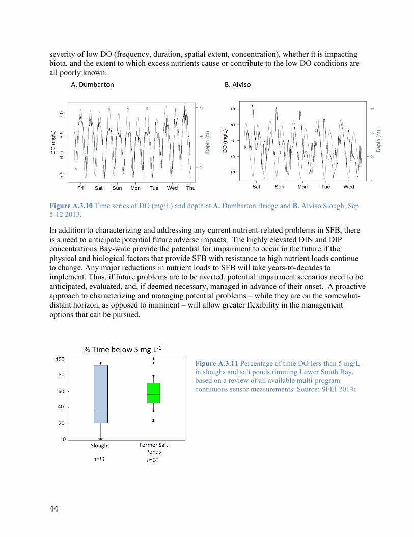
44
severity of low DO (frequency, duration, spatial extent, concentration), whether it is impacting biota, and the extent to which excess nutrients cause or contribute to the low DO conditions are all poorly known.
Figure A.3.10 Time series of DO (mg/L) and depth at A. Dumbarton Bridge and B. Alviso Slough, Sep 5-12 2013.
In addition to characterizing and addressing any current nutrient-related problems in SFB, there is a need to anticipate potential future adverse impacts. The highly elevated DIN and DIP concentrations Bay-wide provide the potential for impairment to occur in the future if the physical and biological factors that provide SFB with resistance to high nutrient loads continue to change. Any major reductions in nutrient loads to SFB will take years-to-decades to implement. Thus, if future problems are to be averted, potential impairment scenarios need to be anticipated, evaluated, and, if deemed necessary, managed in advance of their onset. A proactive approach to characterizing and managing potential problems – while they are on the somewhat-distant horizon, as opposed to imminent – will allow greater flexibility in the management options that can be pursued.
Figure A.3.11 Percentage of time DO less than 5 mg/L in sloughs and salt ponds rimming Lower South Bay, based on a review of all available multi-program continuous sensor measurements. Source: SFEI 2014c
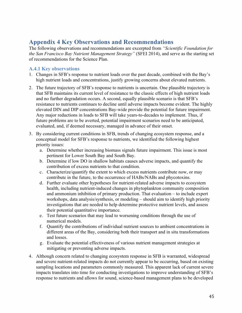
45
Appendix 4 Key Observations and Recommendations The following observations and recommendations are excerpted from “Scientific Foundation for the San Francisco Bay Nutrient Management Strategy” (SFEI 2014), and serve as the starting set of recommendations for the Science Plan.
A.4.1 Key observations1. Changes in SFB’s response to nutrient loads over the past decade, combined with the Bay’s
high nutrient loads and concentrations, justify growing concerns about elevated nutrients.2. The future trajectory of SFB’s response to nutrients is uncertain. One plausible trajectory is
that SFB maintains its current level of resistance to the classic effects of high nutrient loadsand no further degradation occurs. A second, equally plausible scenario is that SFB’sresistance to nutrients continues to decline until adverse impacts become evident. The highlyelevated DIN and DIP concentrations Bay-wide provide the potential for future impairment.Any major reductions in loads to SFB will take years-to-decades to implement. Thus, iffuture problems are to be averted, potential impairment scenarios need to be anticipated,evaluated, and, if deemed necessary, managed in advance of their onset.
3. By considering current conditions in SFB, trends of changing ecosystem response, and aconceptual model for SFB’s response to nutrients, we identified the following highestpriority issues:
a. Determine whether increasing biomass signals future impairment. This issue is mostpertinent for Lower South Bay and South Bay.
b. Determine if low DO in shallow habitats causes adverse impacts, and quantify thecontribution of excess nutrients to that condition.
c. Characterize/quantify the extent to which excess nutrients contribute now, or maycontribute in the future, to the occurrence of HABs/NABs and phycotoxins.
d. Further evaluate other hypotheses for nutrient-related adverse impacts to ecosystemhealth, including nutrient-induced changes in phytoplankton community compositionand ammonium inhibition of primary production. That evaluation – to include expertworkshops, data analysis/synthesis, or modeling – should aim to identify high priorityinvestigations that are needed to help determine protective nutrient levels, and assesstheir potential quantitative importance.
e. Test future scenarios that may lead to worsening conditions through the use ofnumerical models.
f. Quantify the contributions of individual nutrient sources to ambient concentrations indifferent areas of the Bay, considering both their transport and in situ transformationsand losses.
g. Evaluate the potential effectiveness of various nutrient management strategies atmitigating or preventing adverse impacts.
4. Although concern related to changing ecosystem response in SFB is warranted, widespreadand severe nutrient-related impacts do not currently appear to be occurring, based on existingsampling locations and parameters commonly measured. This apparent lack of current severeimpacts translates into time for conducting investigations to improve understanding of SFB’sresponse to nutrients and allows for sound, science-based management plans to be developed

46
and implemented. That said, the considerable amount of time required to implement any management strategy raises the level of urgency such that work should move forward expeditiously.
5. Given the stakes of no action - and the time required for data collection, analysis, andmodeling tools to reach a useable state - work needs to move forward in parallel onimplementing multiple aspects of the Nutrient Strategy. A well-coordinated program isneeded to maximize the effectiveness and efficiency of this effort. That program needs tointegrate seamlessly across what might otherwise be (or become) semi-independent programareas. Specifically, we recommend the following set of highly-integrated program areas:
a. Monitoring: Develop and implement a sustainably-funded and regionally administeredmonitoring program that continues routine monitoring, and fills newly-identified datagaps relevant to nutrients;
b. Modeling: Develop and apply linked hydrodynamic and water quality models tointegrate observations, identify critical data gaps (to be addressed through monitoringor experimental studies), quantify processes at the ecosystem scale, and evaluate futurescenarios (including management alternatives);
c. Observational and Experimental Studies: Undertake special studies (fieldinvestigations, controlled experiments) to address the highest priority knowledge anddata gaps identified in #3; and
d. Data Synthesis and Interpretation: Analysis of existing and newly collected data (frommonitoring and experimental studies), incorporatingmodels, to improve understandingof linkages between nutrients and ecosystem response and to inform the developmentof an assessment framework.
6. The Delta/Suisun boundary, while an important regulatory boundary, is not meaningful fromecological and loading standpoints. Nutrient loads to and transformations within the Deltaexert considerable influence over nutrient loads to and ambient concentrations within Suisun,San Pablo, and Central Bays. Furthermore, the ecology and habitat quality of the Delta andSuisun Bay are tightly coupled. A unified approach – one that spans the Bay-Deltacontinuum - for evaluating the impacts of nutrients on beneficial uses will best serve bothecosystem health in the Bay-Delta and the information needs of environmental managers.
A.4.2 Recommendations for Addressing Priority Knowledge GapsSection A.4.2.1 provides an overview of the recommended highest priority work efforts over thenext 1-5 years to address knowledge and data gaps to, in a targeted way, inform nutrientmanagement decisions in SFB. The process consisted of (see SFEI 2014)• Identifying the highest priority scenarios for potential impairment along one or more
pathways, and high priority science questions that need to be addressed related to thosescenarios (Tables A.4.1 and A.4.2);
• Prioritizing data or knowledge gaps related to the key processes that control ecosystemresponse to nutrients along the pathways of the near-term highest priority scenarios (TablesA.4.3-A.4.6.
Recommendations presented in Section A.4.2.1 are organized around several major themes or types of work. Not all high priority data gaps are discussed in the text below, and the reader is also referred to Tables A.4.1-A.4.6. Section A.4.2.2 takes a broader view, and describes

47
knowledge gaps and data needs in terms of a set of ecological and management challenges that lie ahead.
A.4.2.1 RecommendationsR.1 Develop a regionally-administered and sustainably-funded nutrient monitoringprogramMajor research and monitoring efforts in San Francisco Bay and the Delta include the USGSresearch program4 and the IEP Environmental Monitoring Program.5 The data generated throughthese programs, and the related interpretations, form much of the foundation for currentunderstanding of SFB’s response to nutrients. However, the focus and mandates of theseprograms are not necessarily aligned with those of a program designed program to informnutrient management decisions. Furthermore, future funding of the USGS program is uncertain.
Developing a regionally-administered and sustainably-funded nutrient monitoring program needs to be a major priority. Effort needs to be directed toward developing the institutional and funding frameworks for the program, and developing its primary science goals and activities. Several initial recommendations are presented below.
R.1.1 Program developmentR.1.1.1 Develop institutional and funding agreementsDeveloping and implementing a regional nutrient monitoring program will be a majorundertaking in terms of logistics and cost, and long-term institutional support will be needed.There are several entities currently involved in ship-based and continuous (moored sensors)monitoring (e.g., USGS, IEP, CA Department of Water Resources, CA Department of Fish andGame). To avoid unnecessary duplication of effort and maximize resources, there mayconsiderable advantage to achieving some monitoring program goals through fostering closecoordination among on-going programs, and augmenting those efforts with additionalmonitoring. Activities distributed across independent programs need to be well-coordinated,especially in terms of methods, QA/QC, data management and data sharing, synthesis, andreporting.R.1.1.2 Develop the monitoring program science plan: management questions, goals, priorities,
and approaches A nutrient monitoring program science plan needs to be developed that lays out the management questions, and the program’s goals and priorities relative to those management questions. Detailed plans for achieving those goals also need to be developed. A number of the goals and data needs may differ considerably from those of the current research and monitoring activities (i.e., USGS, IEP). When evaluating the future program’s needs relative to current efforts, particular attention needs to be given to the following issues: • The optimal distribution of effort and resources among broad monitoring categories (water
column vs. benthos, shoals vs. channel, open bay vs. margins, physical/hydrodynamic vs.biological vs. chemical)
• Key parameters or processes to be measured within these categories;• Spatial and temporal resolution of sampling; and
4 http://sfbay.wr.usgs.gov/access/wqdata/ 5 http://www.water.ca.gov/iep/activities/emp.cfm

48
• The distribution of monitoring effort between ship-based sampling and moored sensors forcontinuous monitoring.
For some of these issues, considerable data resources already exist from long-term monitoring in SFB. A major component of the monitoring program design effort should include analyzing this data to inform decisions (e.g., about the necessary spatial and temporal density of sampling). Pilot studies should also be part of planning, to inform which parameters provide important additional information, test methods that provide less expensive approaches for essential data collection, and select moored sensor sites and parameters.
R.1.2. Initial monitoring program science recommendationsSeveral clear monitoring program recommendations emerged through developing the conceptualmodel (SFEI 2014), and identifying data/knowledge gaps related to priority scenarios (Tables6.3-6.6).R.1.2.1 Continue shipped-based monitoring along SFB’s deep channelThe long-term record provided by the USGS research program has yielded important insightsinto the mechanisms that shape SFB’s response to nutrients, including physical and biologicalprocesses that regulate that response, and how that response has changed over time. Maintainingand building upon this program will be critical for anticipating future changes, and for assessingthe effectiveness of any management actions. New parameters may be needed informative, suchas size-fractionated chl-a and C:chl-a, organic forms of N and P, as well as others noted below.R.1.2.2 Develop a moored sensor sub-program for high temporal resolution dataData collection at higher temporal resolution for chl-a, DO, nutrients, turbidity, and otherparameters is needed at multiple locations to assess condition and to improve our quantitativeunderstanding of ecosystem response to nutrients, including the processes that influencephytoplankton blooms, influence oxygen budgets, and regulate nutrient fate. High temporalresolution data will be essential for accurately calibrating water quality models. Continuousmonitoring with moored sensor systems is feasible for a wide range of water quality parameters.Techniques for some parameters are becoming increasingly well-established and reliable (e.g.,salinity, T, turbidity, chl-a, DO), while others are advancing (e.g., nitrate, phosphate, ammonium,phytoplankton counts and identification). Moored sensor systems can telemeter data, allowingfor near real-time assessment of conditions. The data from moored sensors are not a substitutefor ship-based sampling, but rather provide strongly complementary information about physicaland biological processes that influence key water quality parameters (chlorophyll, DO, T, SpC)over time-scales (hours) that are too short to effectively monitor or study through ship-basedsampling. While there are currently multiple stations in Suisun Bay and the Delta that measuresome nutrient-related parameters, there are only 3 newly-added stations south of the Bay Bridgefor measuring chl-a or nutrients (added in September 2013), and few that measure DO and otherparameters (T, SpC, turbidity).
R.1.2.3 In addition to monitoring along the channel, monitoring is needed in shoalenvironments, including lateral transects
Sampling along the shoals is needed for improved understanding of phytoplankton and nutrient processes, and for model calibration. Most of the water quality data available in SFB is from stations along the deep channel. The shoals are important areas for phytoplankton and MPB production, and large lateral heterogeneities in phytoplankton biomass (and SPM, which influences light availability and growth rates) are common in SFB (Thompson et al., 2008;

49
Cloern, 1995). In addition, a substantial proportion of nutrient transformations likely take place along the shoals (benthic nitrification and denitrification). Shoal monitoring can be accomplished both through boat/ship-based transects or with moored sensors, and the best approach will vary depending on the questions being addressed. Using autonomous underwater vehicles (AUVs) outfitted with sensors may also be a possibility. AUVs are commonly employed in research studies, and some AUV-sensor systems are already commercially-available. Pilot studies that test AUVs in SFB would be useful for assessing the feasibility and cost effectiveness of this approach, and to inform planning.
R.1.2.4 Coordinated monitoring in shallow subtidal habitats.Some agencies (e.g., stormwater, wastewater) carry out periodic monitoring in shallow habitats,and several focused studies have been conducted in Lower South Bay systems (Thebault et al.,2008; Shellenbarger et al. 2008; Topping et al., 2009). However, there is currently no systematicmonitoring in shallow margin habitats either at the subembayments scale or Bay-wide. Datacollection on productivity (e.g., chl-a, light levels) and DO concentrations in select systemswould help inform whether adverse impacts are occurring in these systems due to low DO, andhelp ascertain the causes of low DO. Before embarking on this effort, it would be worthwhile toexamine existing data from current or recent studies (e.g., studies in LSB) to assess the need formonitoring and identify the best approaches to pursue.
R.1.2.5 Increased focus HAB/NAB-forming species, phycotoxins, and phytoplankton communitycomposition in general
Given the prevalence of HAB-forming organisms in the Bay and the frequent detection of phycotoxins Bay-wide, it would be prudent to more closely monitor phytoplankton composition, the occurrence of HAB-forming organisms and phycotoxins within San Francisco Bay. Composition and biovolume data collected for HAB-related work would also support assessment and improved mechanistic understanding of other hypothesized nutrient-related shifts in phytoplankton community composition. The abundance and forms of nutrient are two among many factors that can influence phytoplankton community composition and the occurrence of HABs. The relative contributions of those factors toward causing adverse shifts in composition or HAB occurrences are poorly understood. More frequent (in space and time) analysis of phytoplankton composition and phycotoxins, in combination with special studies, (see Recommendation 4.1) will be needed to better understand these mechanisms and assess potential linkages to nutrients.
Determining taxonomy and biomass by microscopy is expensive and time consuming, which limits the amount of data that can be collected. Some amount of manual microscopy ground-truthing will always be needed. However, other techniques, in combination with microscopy, may allow for increased data collection of at lower costs. Carrying out pilot studies will help inform which techniques provide valuable and cost-effective information. Measuring phytoplankton-derived pigments is one such approach. Different classes of phytoplankton have distinct pigment fingerprints. It is possible, with sufficient calibration (relative to microscopy) and training of software to quantify phytoplankton biomass within specific classes. Flow cytometers and digital imaging tools are also available. These systems - which measure optical properties and capture images of individual cells, and employ image-recognizing software to identify and count phytoplankton down to the species level - can be deployed at moored stations for continuous monitoring, used on a monitoring vessel as it cruises along a transect, or used in the laboratory. Moored applications can telemeter data, allowing for near real-time information.

50
One such system provided early warning of a toxic algal bloom in the Gulf of Mexico.6 An additional advantage of digital imaging approaches is that an archive of phytoplankton image data would be developed: if a phytoplankton species eventually becomes important, the digital archive could be mined to determine when that species first appeared.
Pilot projects have been initiated recently that are measuring phycotoxins in SFB, and an algal pigment pilot study is underway. Continuation of similar pilot studies, and testing a variety of methods, will help identify the most informative and cost-effective options, all the while establishing baseline concentration data against which future data can be compared. The feasibility of measuring algal toxins in archived benthos samples should also be considered in order to generate longer time series of algal toxins and look for changes over the past decade or more (if well preserved samples exist).
R.1.2.6 Benthos monitoring to quantify spatial, seasonal, and interannual variability in grazerabundance
Grazing by benthic filter feeders is considered to be one of the main controls on phytoplankton biomass accumulation in several subembayments. To estimate the influence of the benthic grazing, and track its changes in space and time, benthos surveys are needed on a regular basis in some subembayments, most importantly Lower South Bay, South Bay, San Pablo Bay, and Suisun Bay. In recent years there has been ample benthos monitoring in Suisun Bay and the Delta (and some in San Pablo Bay), although the fate of this program is not known. There are currently no sustained programs in the other subembayments. However, there are some years during which intensive benthic sampling has taken place (e.g., Thompson et al. 2008), and along with opportunistic sampling efforts (in some cases, samples have been archived but not yet analyzed for biomass; J Thompson, personal communication). Benthos monitoring could occur less frequent than water quality monitoring, e.g., three times per year (spring, summer, fall). Sorting, counting, and weighing benthos samples is time consuming and costly. A pilot study to test the feasibility of using benthic cameras may also be worth considering (alongside traditional sample collection for calibration/validation), since its use could potentially allow for more cost-effective benthos surveys. R.1.2. 7 Zooplankton abundance/compositionMonitoring data on zooplankton are needed to quantify pelagic grazing rates. Zooplanktonabundance and composition may also serve as an important indicator of food supply and qualityfor higher trophic levels. Long term zooplankton monitoring has been carried out in Suisun Bayand the Delta. However, zooplankton abundance and composition are not currently measured inother subembayments.R.1.2.8 Allocate sufficient funding for data interpretation and synthesisData analysis and data synthesis are essential components of a monitoring program. Allocatingsufficient funds for these activities will allow field results to be efficiently translated intomanagement-relevant observations that inform decisions, and allow the monitoring program tonimbly evolve to address emerging data requirements. Annual reports will be needed that notonly compile and present data, but that also evaluate and interpret trends. More detailed specialstudies will also be needed periodically to generate scientific synthesis reports on complex datasets (e.g., spatial and seasonal trends in phytoplankton community composition).
6 http://www.whoi.edu/oceanus/viewArticle.do?id=46486

51
R.2. Develop and implement a science plan for SFB that targets the highest prioritymanagement and science questionsThe size of SFB, and the complexity and diversity of its nutrient-response issues, create asituation in which there are numerous science questions that need to be addressed to improve ourunderstanding of the system. Addressing the management and science questions will require acombination of field studies, controlled experiments, monitoring, and modeling across the topicsof nutrient cycling, phytoplankton response (biomass and community composition), andhydrodynamics. It will not be feasible to explore all the relevant science questions – that wouldtake longer than management decisions can wait, and would outstrip any reasonable budget. Tobest target science efforts, there would be considerable benefit to developing and implementing ascience plan that: identifies the highest priority management issues, and associated sciencequestions; and identifies the sets of studies and data collection/monitoring needs that efficientlytarget those questions. In some cases, the management issues, science questions, data gaps, andstudies may be similar Bay-wide. In other cases, the science questions or data gaps may besubembayment- or habitat-specific. The science questions listed in Tables A.4.1-A.4.2 and therecommendations in this section could serve as a starting point in what would be an iterativeScience Plan development process.
Analysis of existing data from SFB, combined with broader critical literature review, would be useful early steps in science plan development, to articulate what is well-understood - in other estuaries and SFB - and focus scientific studies and monitoring on addressing the most critical knowledge and data gaps.
R.3. Develop hydrodynamic, nutrient cycling, and ecosystem response modelsTables A.4.1-A.4.2 illustrate that modeling will play a central role in addressing a wide range ofscience questions. Models can also be used to prioritize data collection needs. While there aremultiple hydrodynamic models available for SFB, there are currently no integratedhydrodynamic-phytoplankton-nutrient models. Considerable progress could be made towardaddressing several important science questions through using “simplified-domain” models thatare built upon simplified (spatially-aggregated), but still accurate, hydrodynamics. Potentialapplications of these simplified domain models include (not an exhaustive list):R.3.1 Quantitative analysis of nutrient budgets (including losses/transformations of nutrients);R.3.2 Quantifying the relative importance of major processes that control primary production in
Suisun Bay (light, clams, flushing, NH4+ inhibition), and explore which factors may
explain the changes in phytoplankton biomass in South Bay over the past ~20 years. R.3.3 Performing sensitivity/uncertainty analysis, and identifying highest priority monitoring
activities, process level studies, or rate measurements to minimize model uncertainty. R.3.4 Forecasting ecosystem response under future scenarios, and narrowing the list of high
priority scenarios;
In developing such models, there is a benefit to “starting simple”, and adding complexity as needed. LSB/South Bay and South Bay could serve as good initial focus areas for basic model development and application, because of the abundance of data for those systems and since these two subembayments are where concerns about adverse impacts from nutrients are greatest. Lessons learned through applying basic models will be useful for informing larger-scale or more complex model development.

52
Higher spatial resolution models, or larger spatial scale models (e.g., full Bay as opposed to individual subembayments) will be needed to explore several important issues, including: R.3.5 Determine the zones of influence of individual POTWs under a range of hydrodynamic
forcings and estimated transformations/losses R.3.6 Test future scenarios under which adverse impacts may develop Bay-wide or in
individual subembayments R.3.7 Evaluate the effectiveness of different nutrient control strategies for achieving desired
reductions in ambient concentrations as a function of space and time. R.3.8 Quantify loads from the Delta to Suisun Bay under seasonally- and interannually-varying
hydrological conditions, and the influence of these loads in Suisun and down-estuary subembayments under a range of forcings.
R.3.9 Quantify the importance of net nutrient loads from the coastal ocean to SFB under arange of commonly-occurring forcing scenarios, and explore the fate of the nutrient-rich SFB plume leaving the Golden Gate, and the potential influence of those nutrients on coastal ecosystems.
R.4. Carry out special studies to address key knowledge gaps about mechanisms thatregulate ecosystem response, and inform whether or not impairment is occurringThe draft list of priority science questions in Tables A.4.1-A.4.2, viewed alongside thedata/knowledge gap priorities in Tables A.4.3-A.4.6, present an initial picture of the types of datacollection and studies that are the most important in the near term. A number of priorities havebeen discussed above in the context of monitoring program development (R.1.2.1-1.2.8) andmodeling (R.3.1-R.3.9). An overview of special study priorities is provided below; however, thereader is also referred to the Tables A.4.1-A.4.6.Nutrient cycling R.4.1 Controlled field/lab experiments to measure pelagic nutrient transformations (pelagic
nitrification, nutrient uptake rates) R.4.2 Controlled field/lab experiments to measure benthic nutrient transformations (benthic
nitrification, denitrification, mineralization and N and P fluxes from sediments) R.4.3 Quantify the importance of internal nutrient transformations using models.Productivity of phytoplankton and MPBR.4.4 Controlled experiments that further test the proposed “NH4
+-paradox” mechanism oflower productivity when NH4
+ is elevated, determine relevant thresholds, and allow its effect to be better parameterized and compared to other regulating factors in models (R.3.2).
R.4.5 Through analysis of existing data or through field studies, assess the variability oruncertainty in the Cole and Cloern (1987) productivity relationship due to factors such as different phytoplankton assemblages, temperature, light levels, etc.
R.4.6 Field measurements to quantify MPB primary production rates and biomass.R.4.7 Compare MPB production and biomass with phytoplankton production and biomass,
consider how MPB’s relative importance would change (or already has changed) due to ecosystem change (lower suspended sediments, benthic grazers), and explore how those changes influence nutrient cycling, oxygen budgets, and food webs.

53
Dissolved O2 R.4.8 Controlled field experiments to quantify sediment oxygen demand in a range of
depositional environments. These can be carried out in conjunction with the benthic nutrient transformation special studies as part of the same experimental protocol (R.4.2).
R.4.9 Monitoring and targeted mechanistic studies of DO in shallow margin habitats to assessthe severity of low DO (concentration, spatial extent, frequency, duration).
R.4.9 In cooperation with other efforts or as special nutrient-related studies, determine thedegree to which low DO in margin habitats (or in open water areas of some areas of the Bay, specifically LSB) adversely impact biota. To a certain degree, this work could be carried out based on existing data from other studies on DO tolerances of key organisms. Field surveys of fish or benthos abundance may also be warranted.
R.4.10 Through field experiments and modeling, quantify the degree to which anthropogenicnutrients contribute to occurrences of low DO.
HABs, toxins, and phytoplankton community composition R.4.12 Rigorous analysis of existing phytoplankton community composition data – for HAB-
forming species and composition more broadly – to test qualitative and quantitative agreement with various conceptual models, and refine those conceptual models as needed.
R.4.13 Field studies (collecting phytoplankton composition data at higher temporal or spatialresolution) to test mechanisms of HAB development and phytoplankton community succession in response to physical, chemical, and biological drivers.
R.4.14 Field studies to evaluate the potential importance of salt ponds as incubators of HAB-forming species.
R.4.15 Controlled experiments, using mixed cultures and monocultures from SFB, thatmechanistically explore the interactive effects of nutrient availability (including variability in concentrations and forms), light, and temperature on HAB/NAB development and phycotoxins production, or other shifts toward assemblages that poorly support food webs. The goals of such studies would be to identify conditions that favor some classes or species of phytoplankton over others under the prevailing conditions in SFB (light limitation, excess nutrients), and enable predictions about assemblage response. Such information is also essential for identifying nutrient concentrations or loads that would decrease the risk of HAB occurrences or other adverse assemblage shifts.
R.4.16 Apply the information from R.4.1.5 within models to, among other issues, evaluate themagnitude of the nutrient component of stress, and explore potential composition responses to changing conditions, including those due to potential management actions (e.g., nutrient load reductions).
A.4.2.2 Grand ChallengesDuring the conceptual model development and identification of knowledge gaps, data gaps, andmonitoring needs, four so-called “Grand Challenges” emerged related to understanding andmanaging SFB ecosystem health. While there is overlap between the underlying managementissues that motivated the more specific recommendations above and those that motivated theGrand Challenges, the Grand Challenges represent a somewhat different, more holisticperspective or framework for considering science and data collection needs. In so doing they

54
highlight connections between nutrient issues and other ecosystem health concerns, and provide an additional impetus for addressing those data collection needs.
Grand Challenge 1: What do we need to know in 10-20 yrs to make improved decisions related to water quality management or ecosystem health, including those related to nutrients? 1-2 decades is approximately the time scale over which large capital improvement projects are planned and implemented. 10-20 years is also a long enough time period for trends to become evident, e.g, the changes in phytoplankton biomass in South Bay and LSB since the late 1990s. What information needs to be collected now, to serve as baseline condition data, so that changes in important indicators can be confidently identified and attributed to the correct causal agent(s), whether those changes lead to improved or worsened condition?
Grand Challenge #2: The northern estuary is poised to experience major changes due to management actions and environmental change. Anticipated changes include: nitrification and nutrient load reductions at Sac Regional wastewater treatment plant; numerous large scale restoration projects and changes in water management in the Delta; changing climate patterns altering the timing, residence time, and amount of water passing through the Delta. What do we need to be measuring now in order to determine if these changes have positive, negative, or no impacts on ecological health in SFB and the Delta? How will phytoplankton respond to changes in nutrient loads/speciation? How will the food web respond?
Grand Challenge #3: Large areas along the margins of South Bay and LSB are slated to undergo restoration. Given the size of these areas compared to the adjacent water surface area, it is reasonable to expect that proposed restorations along the margins will have measurable impacts on water quality and ecological health in the open Bay. Some of these effects may be positive, including increased habitat for fish, birds and other organisms. It will be desirable to document those changes; in order to do so, baseline data is needed for these higher trophic level indicators of ecosystem health. Those changes could also encourage more denitrification and decreased N within the Bay, which could be considered within integrated nutrient management plans. As discussed earlier, there may also be unintended and undesirable consequences, including: restored/reconnected salt ponds acting as incubators for HAB-forming phytoplankton species; exceedingly high primary production rates and high biomass, causing periodic low DO in wetlands and sloughs; and increased duration of stratification due to dampening of tidal mixing energy. What hypotheses of adverse impacts need to be tested, as part of restoration planning, so that the risks of severe unintended consequences can be minimized?
Grand Challenge #4: Similar to Grand Challenges 1-3, what baseline observational data is needed to detect climate-related changes in habitat quality in SFB and to disentangle them from other anthropogenic drivers? What types of modeling simulations should be done to anticipate effects? The CASCaDE II7 project is exploring these issues, largely focused in the Delta. Similar studies may be warranted in the Bay.
7 http://cascade.wr.usgs.gov/
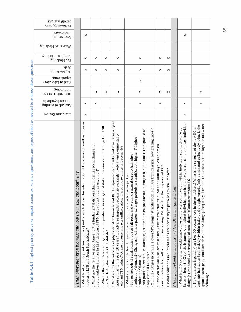
55
Tab
le A
.4.1
Hig
hest
prio
rity
adve
rse
impa
ct sc
enar
ios,
scie
nce
ques
tions
, and
type
s of s
tudi
es n
eede
d to
add
ress
thos
e qu
estio
ns
Literature Review
Analysis of existing data and synthesis
Data collection and monitoring
Field or laboratory experiments
Bay Modeling: Basic
Bay Modeling: Complex or full bay
Watershed Modeling
Assessment Framework
Technology, cost-‐benefit analysis
1 High phytoplankton biom
ass and low DO in LSB and South Bay
a. What level of phytoplankton biomass (and over what area, for w
hat period of time) would result in adverse
impacts in LSB and South Bay habitats?
x x
x x
x
b. What are the relative importances of the fundam
ental drivers that underlie recent changes in
phytoplankton biom
ass in LSB (decreased SPM
, loss of benthic grazers, other)?
x
x
x x
c. What is the im
portance of organic matter produced in margin habitats to biomass and DO budgets in LSB
and South Bay deep subtidal habitats?
x
x x
d. What w
ill be the response of phytoplankton biomass and DO if suspended sediments continue decreasing at
rates similar to the past 20 years? Do adverse impacts becom
e increasingly likely at environmentally-‐
relevant SPM
values? Or are adverse im
pacts unlikely along this pathw
ay under this scenario?
x
x x
e. What scenarios could lead to worsened conditions and adverse im
pacts?
-‐ Longer periods of stratification due to salt pond and wetland restoration efforts, higher
production/biom
ass? -‐ Changes in climate patterns, longer periods of stratification, higher T, higher
production/biom
ass?
-‐ Salt pond and wetland restoration, greater biomass production in margin habitats that is transported to
deep subtidal habitats?
-‐ Multiple changes in parallel (lower SPM
, longer stratification, biomass from margins, low
grazing rates)?
x
x x
x x
f. Based on this analysis, what are likely future trajectories in LSB and South Bay? Will biomass
concentrations level off or continue increasing? W
hat w
ill be the response of DO?
x
x
x x
g. What reductions in nutrient loads are necessary to prevent adverse im
pacts?
x
x x
2 High phytoplankton biom
ass and low DO in margin habitats
a. What low
DO ‘severity’ would cause adverse im
pacts: spatial extent w
ithin individual sub-‐habitats (e.g.,
%age of slough), DO deficit, frequency, duration? Individual sub-‐habitats vs. overall condition (e.g., individual
slough(s) impacted vs. percentage of total slough kilometers impacted)?
x x
x
b. How
com
mon (spatially) are low DO occurrences in these habitats? W
hat is the severity of the low DO in
each sub-‐habitat and collectively (within individual sloughs/creeks/salt-‐ponds, and collectively, what is the
spatial extent (e.g., small stretch vs. entire slough), frequency, duration, DO deficit, bottom layer or full water
column)?
x
x

56
Literature Review
Analysis of existing data and synthesis
Data collection and monitoring
Field or laboratory experiments
Bay Modeling: Basic
Bay Modeling: Complex or full bay
Watershed Modeling
Assessment Framework
Technology, cost-‐benefit analysis
c. Are relevant biota adversely im
pacted by low DO? Field surveys, potentially controlled studies. Avoidance,
stress/toxicity, death
x x
x x
d. What m
echanisms act to cause the periodicity of low
DO, including causing it to develop and dissipate? N
ew
organic matter sources (e.g., in situ production within sloughs or inputs from adjacent habitats,
microphytobenthos vs. phytoplankton), on-‐going sediment oxygen demand, residence tim
e, stratification,
freshw
ater inputs, tidal exchange
x
x x
x x
e. To what extent do anthropogenic nutrient loads contribute to or cause increased severity of low
DO (spatial
extent, DO deficit, frequency, duration)?
x
x
x
f. Based on observed (or m
odeled) conditions relative to conditions that have adverse impacts, are these
habitats (subset or as a whole) adversely im
pacted by low DO?
x
x
x x
x
3. HABs/NABs and phycotoxins
a. What frequency or m
agnitude of HABs/NABs or H
AB-‐toxins w
ould cause adverse im
pacts?
x x
x
x
b. How
do the abundances of phycotoxins and the HAB-‐forming species vary in space and tim
e within the
Bay? Have there been detectable changes over time, based on existing data? W
hat are the sources of
phycotoxins (in situ production vs. transport into SFB or subem
baym
ents)?
x
x x
c. What causes/contributes to increased frequency or elevated abundances of HAB/NAB-‐forming organisms?
To what extent do nutrients cause, contribute to, or enable increased abundance/blooms? Seeding rates from
the coast, seeding rates from adjacent habitats (including salt ponds), role of physical drivers (T, light,
mixing/stratification) and chemical conditions (nutrients) favoring higher in situ production specifically of
HAB/NAB forming organisms
x
x x
x x
d. What causes/contributes to production of in situ phycotoxins production? To what extent do nutrients
cause, contribute to, or enable increased phycotoxins production? role of physical drivers (T, light,
mixing/stratification) and chemical conditions (nutrients) favoring higher in situ production
x
x x
e. What future scenarios could increase the frequency or severity of HAB/NAB events or increase phycotoxin
abundance?
-‐ restoration and reconnection of salt ponds/wetlands? high-‐light, warm, nutrient-‐replete incubators?
-‐ future water managem
ent practices in the Delta (w
ithdrawals, longer residence tim
es) ?
-‐ changes in clim
ate patterns? H
ow likely are those changes in the 20-‐30 yr time horizon?
x
x x
x

57
Literature Review
Analysis of existing data and synthesis
Data collection and monitoring
Field or laboratory experiments
Bay Modeling: Basic
Bay Modeling: Complex or full bay
Watershed Modeling
Assessment Framework
Technology, cost-‐benefit analysis
h. Based on a comparison of observed conditions and conditions considered to induce adverse im
pacts, are
regions/subembaym
ents/habitats of SFB experiencing HAB/NAB related adverse impacts, or will they in the
future?
x
x
i. What decreases in nutrient loads or ambient nutrient concentrations would decrease adverse impacts, or
the risk of adverse im
pacts, from
HABs/NABs?
x x
4. Other Nutrient Impact Pathways: Low phytoplankton biomass (NH4+ inhibition),
Suboptimal phytoplankton com
munity com
position
a. What is the underlying mechanism by which NH4+ slow
s or inhibits primary production? Characterize NH4+
concentrations and magnitude of effect. At w
hat NH4+ concentrations are primary production rates
substantially im
pacted?
x x
x
b. What is the relative contribution of elevated NH4+ com
pared to other factors that m
aintain low
phytoplankton biom
ass in Suisun Bay (clam grazing, light limitation, flushing)?
x x
c. Are current NH4+ loads or concentrations adversely im
pacting biom
ass levels in Suisun Bay?
x
x
x x
x
d. What nutrient load reductions would prevent or m
itigate adverse im
pacts due to NH4+ inhibition of primary
production?
x x
e. What constitute optimal, or healthy, phytoplankton assem
blages in SFB’s subembaym
ents? Conversely,
what assem
blages would be considered to poorly support desirable food webs?
x x
x
f. How
have phytoplankton community com
positions changed within SFB subembaym
ents over recent years?
x
x
g. Based on what is known from
other system
s or from prior experimental/field work (Bay-‐Delta or
elsewhere), what hypothesized mechanisms are most likely to influence phytoplankton com
munity
composition in the Bay-‐Delta, based on am
bient conditions (nutrient concentrations, light, tem
perature,
stratification, etc.)? W
hat controlled experiments or observations in SFB are needed to further evaluate these
proposed mechanisms in SFB?
x x
h. What is the magnitude (or relative importance) of the role that current ambient nutrient concentrations
play in shaping phytoplankton community com
position?
x x
x
x x
i. What changes to nutrient availability would mitigate or prevent adverse im
pacts of nutrients on
phytoplankton community com
position?
x x
x
x x
i. What other adverse im
pact pathw
ays m
ay require further attention in SFB (aquatic macrophytes,
macroalgae, SAV habitat)?
x x

58
Tab
le A
.4.2
Hig
hest
prio
rity
miti
gatio
n sc
enar
ios,
scie
nce
ques
tions
, and
type
s of s
tudi
es n
eede
d to
add
ress
thos
e qu
estio
ns
Literature Review
Analysis of existing data and synthesis
Data collection and monitoring
Field or laboratory experiments
Bay Modeling: Basic Bay Modeling: Complex or full bay/Delta
Watershed Modeling:
Assessment Framework
Technology, cost-‐benefit analysis
5. Reductions in nutrient loads from
POTWs and nutrient loads from
the Delta
a. What are the magnitudes of loads from
individual POTWs?
x
x
c. How
do internal processes shape nutrient concentration within SFB, how
do they vary in space/tim
e:
mixing/flushing, nitrification, denitrification, uptake/assimilation, regeneration from
sediments, etc.
x
x x
b. What are the zones of influence and magnitude of contributions of individual POTWs and Delta loads, and
how do these vary seasonally and interannually?
x x
d. How
do Delta loads to Suisun Bay vary seasonally and interannually? W
hat portions of the loads that enter
Suisun Bay from
the Delta originate from
Regional San, others POTWs? What portions of the loads com
e from
Central Valley agriculture? W
hat are the load contributions from
agriculture within the Delta?
x
x
x x
x
f. What w
ill Delta loads to Suisun Bay be under future scenarios: restoration, changes to water managem
ent
practices, changes in agricultural practices?
x x
i. Considering areas of influence, zones where im
pairment m
ay be occurring, and internal processes, what
combination of load reductions are needed to mitigate or prevent im
pairment?
x x
g. What is the range of options for achieving various levels of nutrient load reductions from
POTWs? W
hat are
the costs and multiple benefits (nutrients + other benefits, e.g., recycled water) of individual POTW efforts,
and of longer-‐term integrated sub-‐regional plans?
x
h. Given the necessary load reductions and cost-‐benefits, what are the best options for achieving load
reductions?
x
6. Reductions in stormwater nutrient loads
a. Are stormwater nutrient loads potentially im
portant sources to some margin habitats in some
subembaym
ents, or at the subembaym
ents scale, and do they warrant further consideration?
x
x
x x
x
b. If yes, what are the loads from priority watersheds? What is their contribution to nutrient loads, or organic
matter/BOD loads, to margin habitats?
x
x
x
c. What are the magnitudes of stormwater nutrient contributions to deep subtidal habitats in other
subembaym
ents?
x x

59
Literature Review
Analysis of existing data and synthesis
Data collection and monitoring
Field or laboratory experiments
Bay Modeling: Basic Bay Modeling: Complex or full bay/Delta
Watershed Modeling:
Assessment Framework
Technology, cost-‐benefit analysis
7. Other mitigation strategies: wetland restoration/treatment and shellfish beds
a. What is the potential for wetland restoration/treatment to mitigate adverse im
pacts of nutrients?
x
x x
b. What is the potential for managed shellfish beds to mitigate adverse im
pacts of nutrients?
x
x x
b. If wetlands or m
anaged shellfish beds appear to be promising nutrient managem
ent options – what do pilot
studies, advanced modeling, and economic considerations suggest about their potential to be part of an
integrated managem
ent program
?
x
x
x
8. Influence of nitrification at Regional San and Suisun direct POTWs on NH4+ inhibition of
primary production or other adverse impacts
a. What is N
H4+ fate within the Delta and how
does this change as a function of season, flow, etc.?
x x
b. What load reductions are necessary to reduce NH4+ to ambient concentrations that would not inhibit
production or have other adverse im
pacts?
x x

60
Tab
le A
.4.3
N a
nd P
load
s and
cyc
ling:
cur
rent
stat
e of
kno
wle
dge
for k
ey p
roce
sses
and
par
amet
ers
Process or Param
eters
Importance for
quantitative
understanding
Current Level of Knowledge about m
agnitude, com
position,
or controls
Need for
additional or
continued data
collection, process
studies, modeling
Priority for
study in next
1-‐5 years
Loads
POTW
s High
Moderate: Com
prehensive effluent monitoring is currently
underway. Prior to 2012, data availability varies by POTW
and
in general is fairly sparse for several nutrient forms (NO3-‐, o-‐
PO4, TN, TP)
Very High
Very High
Stormwater runoff
Uncertain
Low: Limited stormwater data and lim
ited modeling effort
High
High
Delta
High
Low: Initial estimates suggest Delta loads m
ay be a large source
but they need to be validated, and time-‐series of loads are
needed.
Very High
Very High
Groundwater
Low
Low: Poorly quantified but not expected to be major source because of
relatively high loads from other sources
Low
Low
Direct atmospheric
deposition
Low
Low: Poorly quantified but not expected to be major source because of
relatively high loads from other sources, including from
the large
Central Valley watershed
Low
Low
Exchange through GG
Uncertain
Low: Has the potential to be large, but highly uncertain
High
High
Processes
Benthic denitrification
High
Low: see OM mineralization and NH4 and PO4 release below
Very High
Very High
Pelagic denitrication
Low
Low: not expected to be important because of oxic water colum
n Low
Low
Benthic nitrification
High
Low: see OM mineralization and NH4 and PO4 release below.
Potentially large, but limited field measurements, and need for
both field and model-‐based estimates.
Very High
Very High
Pelagic nitrification
High
Low: Potentially large, but limited field measurements, and need
for both field and model-‐based estimates.
Very High
Very High
N fixation
Low/Uncertain
Low
Moderate
Low

61
Process or Param
eters
Importance for
quantitative
understanding
Current Level of Knowledge about m
agnitude, com
position,
or controls
Need for
additional or
continued data
collection, process
studies, modeling
Priority for
study in next
1-‐5 years
OM mineralization and
release of NH4 and o-‐PO4
from
sediments, and in the
water colum
n
High
Low: Potentially a substantial source from
the sediments to the water
column. Limited data from
two studies in SFB, but well-‐studied in other
system
s and at least initially may be able to use that information. Field
studies aimed at exploring this issue will also inform sediment oxygen
demand, benthic primary production, benthic denitrification, and
benthic nitrification.
Very High
Very High
Settling/burial of N and P
High
Low/M
oderate: limited field estimates to date, although could be
estim
ated based on other sedimentation data.
Moderate
Low
Rates of NH4, NO3, and o-‐
PO4 uptake by
phytoplankton
High
Moderate: field measurements exist for N
H4 and NO3 in northern
estuary, limited data in South Bay and LSB. Uptake rates for P are not
well-‐studied. Both N and P uptake rates can be partially constrained by
know
ing phytoplankton C:N:P and productivity
Moderate
Moderate
Other processes: DNRA,
ANAM
OX
Low
Low: but expected to be relatively small
Low
Low
N and P budgets for
subembaym
ents: loads,
transformations,
sources/sinks, export
High
Low: The ability to quantify these will provide im
portant information
on the subembaym
ents’ ability to process/assimilate N and P. Basic
modeling work needed.
Very High
Very High
Ambient concentration data
Phytoplankton C:N:P
High
Low: Currently not routinely measured during monitoring
Very High
Very High
Concentration of NO3, NH4,
and PO4
High
Moderate: monthly data available at ~15 stations Bay-‐wide but finer
spatial and temporal resolution needed to inform process level
understanding and modeling
Very High
Very High
Concentrations of NO 2
-‐ and
N2O
Low/M
oderate
Moderate: not needed for nutrient budgets, but informative as
diagnostic of processes
Moderate
Moderate
Concentration of DON
, PON
, DOP, POP within and
loaded to the system
Moderate/
uncertain
Low: Little current data, and information is needed. Given the
high DIN and DIP concentrations, abundance organic forms m
ay
be relatively low.
High
High

62
Tab
le A
.4.4
Phy
topl
ankt
on a
nd M
PB p
rodu
ctiv
ity /
biom
ass a
ccum
ulat
ion:
cur
rent
stat
e of
kno
wle
dge
for
key
proc
esse
s and
par
amet
ers
Process or Param
eters
Importance for
quantitative
understanding
Current Level of confidence about magnitude or
mechanistic controls
Need for additional
or continued data
collection, process
studies, modeling
Priority
for study
in next
1-‐5 years
PHYTOPLANKTON -‐ Processes
Primary production rates
High
Low/M
oderate: Basic understanding about light limitated production
is well m
odeled. Recent studies suggest that the relationship may have
shifted, and revisiting this may be important for estimating system
productivity.
Very High
High
Pelagic grazing
High
Low: Long-‐term program
in Suisun Bay/Delta for m
acrozooplankton, but
limited micro-‐zooplankton data, which may be more quantitatively
important in terms of overall grazing rate. No system
atic zooplankton
sampling in LSB, South Bay, Central Bay.
Very High
High
Benthic grazing
High
Low: good data to support estimates in Suisun Bay. Limited data in LSB
South Bay. Monitoring of benthos abundance would inform this.
Very HIgh
Very High
Sinking, respiration, burial
High
Moderate: Discussed within context of Dissolved Oxygen
Low
Low
Inhibition of primary
production rates by elevated
NH4+
High/ Uncertain
Low: Several studies have been com
pleted and others are underway.
Uncertainty remains about mechanism and relative importance of the
process. Field/lab studies and modeling work can be done in parallel,
with the former designed to further elucidate the mechanism and
thresholds and the latter to quantify its role relative to other factors.
Very High
Very High
Production in the shoals vs.
channels (during
stratification), and physical
or biological controls on
bloom growth/propagation
High
Low: Considered to be an im
portant process but limited data
available. Data needed to better predict bloom
magnitudes.
Very High
Very High
Germination of resting stages
Low
Low: Not considered am
ong the highest priority processes to
study
Low
Low
PHYTOPLANKTON – Ambient concentration data
High frequency data in
channel
High
Low: Very lim
ited high temporal resolution (continuous) phytoplankton
biom
ass data beyond of Suisun Bay. Needed to better predict bloom
s. Very High
Very High
High temporal resolution
data in shoals
High
Low: Very lim
ited high temporal resolution (continuous) phytoplankton
biom
ass data beyond of Suisun Bay. Needed to better predict bloom
s. Very High
Very High
d High
Moderate/High: USGS program has been collecting monthly data at
along the channel for the past 35 years, and needs to be continued.
Very High
Very High
Phytoplankton C:N ,C:chl-‐a,
High
Low: Valuable information to inform understanding of processes and for
Very High
Very High

63
Process or Param
eters
Importance for
quantitative
understanding
Current Level of confidence about magnitude or
mechanistic controls
Need for additional
or continued data
collection, process
studies, modeling
Priority
for study
in next
1-‐5 years
and size-‐fractionated chl-‐a
modeling
Microphytobenthos -‐ Processes
Primary production rates
Moderate
Low: m
ay be able to predict productivity based on light levels and
chl-‐a, although needs to be confirmed
Moderate
Moderate
Grazing
Moderate/
Unknown
Low: Potentially im
portant as a sink, but difficult to study.
Low
Low
Microphytobenthos – Ambient abundance data
Basic biom
ass information,
seasonal, spatial
High
Low: Very lim
ited data on MPB abundance and productivity,
despite the fact that MPB productivity may be comparable in
magnitude to phytoplankton productivity.
High
High
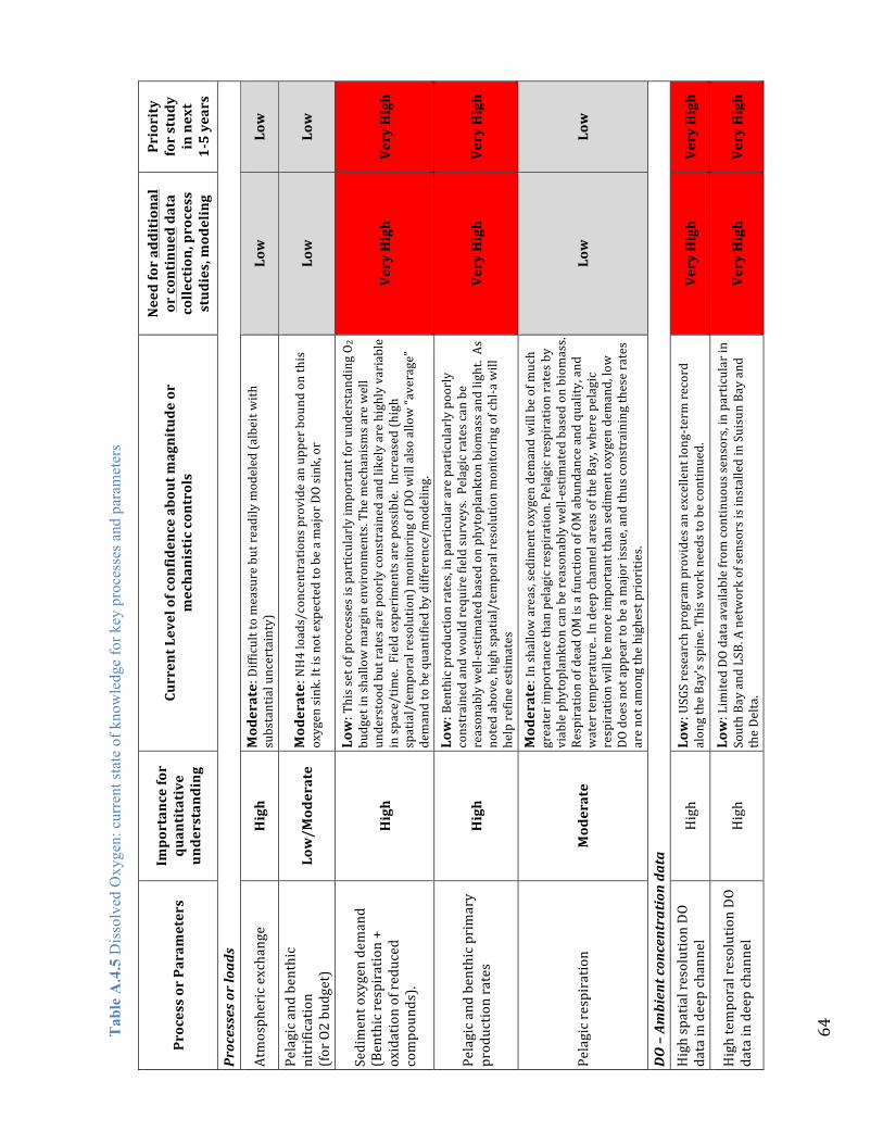
64
Tab
le A
.4.5
Dis
solv
ed O
xyge
n: c
urre
nt st
ate
of k
now
ledg
e fo
r key
pro
cess
es a
nd p
aram
eter
s
Process or Param
eters
Importance for
quantitative
understanding
Current Level of confidence about magnitude or
mechanistic controls
Need for additional
or continued data
collection, process
studies, modeling
Priority
for study
in next
1-‐5 years
Processes or loads
Atmospheric exchange
High
Moderate: Difficult to measure but readily modeled (albeit w
ith
substantial uncertainty)
Low
Low
Pelagic and benthic
nitrification
(for O2 budget)
Low/M
oderate
Moderate: NH4 loads/concentrations provide an upper bound on this
oxygen sink. It is not expected to be a major DO sink, or
Low
Low
Sediment oxygen demand
(Benthic respiration +
oxidation of reduced
compounds).
High
Low: This set of processes is particularly im
portant for understanding O2
budget in shallow margin environm
ents. The mechanisms are well
understood but rates are poorly constrained and likely are highly variable
in space/tim
e. Field experiments are possible. Increased (high
spatial/temporal resolution) monitoring of DO will also allow “average”
demand to be quantified by difference/m
odeling.
Very High
Very High
Pelagic and benthic primary
production rates
High
Low: Benthic production rates, in particular are particularly poorly
constrained and would require field surveys. Pelagic rates can be
reasonably well-‐estimated based on phytoplankton biom
ass and light. As
noted above, high spatial/temporal resolution monitoring of chl-‐a will
help refine estim
ates
Very High
Very High
Pelagic respiration
Moderate
Moderate: In shallow areas, sediment oxygen demand will be of much
greater importance than pelagic respiration. Pelagic respiration rates by
viable phytoplankton can be reasonably well-‐estimated based on biom
ass.
Respiration of dead OM
is a function of OM abundance and quality, and
water temperature.. In deep channel areas of the Bay, where pelagic
respiration will be more important than sediment oxygen demand, low
DO does not appear to be a major issue, and thus constraining these rates
are not among the highest priorities.
Low
Low
DO – Ambient concentration data
High spatial resolution DO
data in deep channel
High
Low: USGS research program
provides an excellent long-‐term record
along the Bay’s spine. This w
ork needs to be continued.
Very High
Very High
High temporal resolution DO
data in deep channel
High
Low: Limited DO data available from
continuous sensors, in particular in
South Bay and LSB. A network of sensors is installed in Suisun Bay and
the Delta.
Very High
Very High

65
Process or Param
eters
Importance for
quantitative
understanding
Current Level of confidence about magnitude or
mechanistic controls
Need for additional
or continued data
collection, process
studies, modeling
Priority
for study
in next
1-‐5 years
High temporal resolution
data in shoals and shallow
margin habitats
High
Low: Som
e special studies have been performed, and some on-‐going
monitoring by POTW
s and others (e.g., USGS studies in salt ponds). W
hile
these individual efforts have valuable information and some reports are
available, a meta-‐analysis of this data has not been completed, and there
is currently no overarching regional program
.
Very High
Very High

66
Tab
le A
.4.6
Phy
topl
ankt
on c
omm
unity
com
posi
tion
and
HA
Bs:
cur
rent
stat
e of
kno
wle
dge
for k
ey p
roce
sses
and
par
amet
ers
Process or Param
eters
Importance for
quantitative
understanding
Current Level of Certainty about magnitude, com
position, or
controls
Need for additional or
on-‐going data
collection or process
studies
Priority for
study in
next
1-‐5 years
Processes
Pelagic grazing rates (size-‐
selective)
High
Low: No system
atic zooplankton sampling in LSB, South Bay, Central Bay.
Only 1 station in San Pablo.
Moderate
Moderate
Size-‐selective benthic grazing
rates
High
Low: Good data to support estimates in Suisun Bay. Limited data in LSB
South Bay. Monitoring of benthos abundance would inform this.
Very High
Very High
Temperature, light, and
nutrient (concentration, N:P,
form of N) preferences of
phytoplankton PFTs specific to
SFB subembaym
ents
High
Low: Limited understanding of how
these factors/preferences m
ay
shape phytoplankton community com
position, in particular in a
light-‐limited nutrient-‐replete system
. Very High
Very High
Effects of trace metals,
organics or pesticides
Moderate/
Uncertain
Low: Limited information on
vitamins, trace-‐metals, and the influence of anthropogenic
contam
inants such as pesticides that may be influencing com
munity
composition.
competition with diatoms.
Moderate
Moderate
Effect of physical forcings,
including exchange between
subembaym
ents, oceanic and
terrestrial (including wetlands,
salt ponds) end-‐mem
ber
inputs, large scale climate
forcings
High
Moderate: Data on com
munity com
position over the past 20 years
(Bay wide) and up to 40 years (Suisun and Delta) to explore
different explanations.
Very High
Very High
NH4 inhibition: diatom
productivity
High/
Uncertain
Low: Several studies com
pleted, others underway.
Very high
Very high
Ambient com
position data
Size-‐fractionated chl-‐a
High
Low: Provides a coarse measure of in which classes phytoplankton
biom
ass resides, which is a useful albeit coarse surrogate for food
quality. Not currently being collected but could be easily added to
monitoring.
HIgh
High

67
Process or Param
eters
Importance for
quantitative
understanding
Current Level of Certainty about magnitude, com
position, or
controls
Need for additional or
on-‐going data
collection or process
studies
Priority for
study in
next
1-‐5 years
Phytoplankton community
composition, monthly time-‐
scales, at sufficiently high
spatial resolution, and higher
temporal/spatial resolution to
test mechanisms
High
Moderate: 20 year near-‐monthly Bay-‐wide record from
USGS and
~40 year record for Suisun and Delta. But few higher resolution
data sets or special studies.
Very high
Very high
Frequency and magnitude of
detection of HABs or H
AB
toxins
High
Low: Limited data on HABs and toxins, and
Very high
Very high
Phytoplankton community
composition in salt ponds,
particularly HAB-‐forming
species
High
Low: Limited data to date, but of high concern.
Very High
Very High
Surrogate measures for
phytoplankton composition
Low
Low: The use of phytoplankton pigments or digital image
recognition approaches could be piloted that would eventually
increase the am
ount of com
position data that could be collected
Very High
Very High